Embed Size (px)
Citation preview

VTT WORKING PAPERS 179
Alpo Ranta-Maunus, Julia K. Denzler & Peter Stapel
Strength of European TimberPart 2. Properties of spruce and pine tested in Gradewood project

ISBN 978-951-38-7521-3 (URL: http://www.vtt.fi/publications/index.jsp) ISSN 1459-7683 (URL: http://www.vtt.fi/publications/index.jsp)
Copyright © VTT 2011
JULKAISIJA – UTGIVARE – PUBLISHER
VTT, Vuorimiehentie 5, PL 1000, 02044 VTT puh. vaihde 020 722 111, faksi 020 722 4374
VTT, Bergsmansvägen 5, PB 1000, 02044 VTT tel. växel 020 722 111, fax 020 722 4374
VTT Technical Research Centre of Finland, Vuorimiehentie 5, P.O. Box 1000, FI-02044 VTT, Finland phone internat. +358 20 722 111, fax +358 20 722 4374

Series title, number and report code of publication
VTT Working Papers 179 VTT-WORK-179
Author(s) Alpo Ranta-Maunus, Julia K. Denzler & Peter Stapel Title Strength of European Timber Part 2. Properties of spruce and pine tested in Gradewood project
Abstract More than 6 000 specimens of spruce and pine grown in several European countries were tested by destructive and non-destructive means in laboratory. Five strength grading machines were also used to test the material. This report includes the description of sampling as well as tension and bending properties of material with comparisons to earlier results.
Main purpose of this report is to document experimental results. Analysis in-cludes basic statistical characteristics such as means, coefficients of variation and correlations between grade determining properties and indicating properties. Also the possibility of having same settings in different countries has been fo-cused.
ISBN 978-951-38-7521-3 (URL: http://www.vtt.fi/publications/index.jsp)
Series title and ISSN Project number VTT Working Papers 1459-7683 (URL: http://www.vtt.fi/publications/index.jsp)
Date Language Pages August 2011 English 67 p. + app. 46 p.
Name of project Commissioned by Gradewood
Keywords Publisher Grading, strength, bending, tension, spruce, pine, machine, test, correlation
VTT Technical Research Centre of Finland P.O. Box 1000, FI-02044 VTT, Finland Phone internat. +358 20 722 4520 Fax +358 20 722 4374


5
Preface
The present report documents experimental research performed in Work Package 3 of the Gradewood-project. Gradewood (Grading of timber for engineered wood products) was a transnational project belonging to the WoodWisdom-net programme. The project was funded by several national funding organizations and industries as a result of the initiative of European wood industries (Building With Wood). The project was lead by a Steering Committee (chair Raimund Mauritz, Doka) and the management of work was lead by a Project Management Group (chair Mattias Brännström, Stora Enso Timber). Background of project and results of analysis of existing data have been published earlier [1].
Experimental work published here was made as co-operation of several organisations and their roles, and roles of the authors were as follows:
1. Technical University of Munich, Peter Stapel: co-ordination of Work Package 3, and testing of 900 timbers from Poland.
2. Holzforschung Austria, Julia K. Denzler: testing of 1 900 timbers from Slovakia, Slovenia, Romania and Ukraine.
3. University of Ljubljana, Goran Turk, and Slovenian National Building and Civil Engineering Institute ZAG: testing of 1 100 Slovenian timbers.
4. FCBA, France, Didier Reuling: testing of 1 000 timbers from France, Poland and Sweden.
5. ETH, Switzerland, Markus Deublein: tension testing of 450 Swiss spruces.
6. SP, Sweden, Rune Ziethén: testing of 400 Swedish timbers.
7. VTT, Tomi Toratti and Alpo Ranta-Maunus: co-ordination of the project, and Mikael Fonselius, tension testing of 400 Finnish and Russian pine timbers.
Following strength grading machine manufacturing companies have tested the material by using their equipments: Brookhuis, CBS-CBT, Luxscan, MiCROTEC and Rosén. Collaboration between research institutes and grading machine companies was so or-ganised that laboratory test results were made available to grading machine companies, and grading machine results were distributed to researchers. The authors
6
Contents Preface ......................................................................................................................... 5
List of symbols .............................................................................................................. 7
1. Introduction ............................................................................................................. 8
2. Materials.................................................................................................................. 9
3. Methods ................................................................................................................ 13 3.1 Overview ............................................................................................................................. 13 3.2 Non destructive testing......................................................................................................... 14
3.2.1 Laboratory testing .................................................................................................. 14 3.2.1.1 Determination of dynamic modulus of elasticity ..................................... 14 3.2.1.2 Knot area measurement........................................................................ 15
3.2.2 Machine testing ..................................................................................................... 15 3.2.2.1 Determination of dynamic modulus of elasticity ...................................... 15 3.2.2.2 Knot measurement ............................................................................... 15 3.2.2.3 Available machine data ......................................................................... 15
3.3 Destructive testing ............................................................................................................... 16 3.3.1 Test methods ......................................................................................................... 16
3.3.1.1 Strength ............................................................................................... 16 3.3.1.2 Modulus of elasticity ............................................................................. 17
3.3.2 Density .................................................................................................................. 17 3.3.3 Adjustments........................................................................................................... 18
3.4 Methods of analysis ............................................................................................................. 19
4. Results .................................................................................................................. 20 4.1 Basic statistical results of ungraded timber ........................................................................... 20
4.1.1 Spruce in bending .................................................................................................. 20 4.1.2 Spruce in tension ................................................................................................... 23 4.1.3 Pine in bending ...................................................................................................... 27 4.1.4 Pine in tension ....................................................................................................... 30 4.1.5 Summary of machine data ..................................................................................... 33
4.2 Bandwidth method results in comparison to earlier data ........................................................ 41 4.2.1 Spruce in bending .................................................................................................. 41 4.2.2 Spruce in tension ................................................................................................... 42 4.2.3 Pine in bending ...................................................................................................... 44
4.3 Properties of in-grade timber ................................................................................................ 44 4.3.1 Grading procedure ................................................................................................. 44 4.3.2 Grading results ...................................................................................................... 52
5. Summary ............................................................................................................... 65
Acknowledgements ..................................................................................................... 66
References ................................................................................................................. 67
Appendix A: Correlation matrices of samples

7
List of symbols
a distance between support and next loading head in bending test
Edyn dynamic modulus of elasticity based on measurement of natural frequency of longitudinal vibration and density, adjusted to u = 12%
Efreq Edyn adjusted to u = 12% assuming constant density = 450 kg/m3
Eglobal modulus of elasticity determined according to EN408 and adjusted to u = 12% in bending over the distance between the supports
Elocal modulus of elasticity determined according to EN408 and adjusted to u = 12% in bending over 5*width between the loading heads in tensionover 5*width
E for bending Elocal if only Elocal has been determined; otherwise 1.3 Eglobal -2690 for tension Elocal
freq first natural frequency
fm bending strength determined according to EN408, adjusted to 150 mm width and a length of 18*width with distance between the supporters of 6*width
ft tension strength determined according to EN408, adjusted to 150 mm width and a length of 9*width
KAR total knot area ratio
L length of specimen
l distance between the supporters (bending) or between the grips (tension)
density determined according to EN408, adjusted to u = 12%
specimen average density of specimen based on weighing by scale, adjusted to u = 12%
450 assumed constant density of 450 kg/m³
specimen average density of specimen based on weighing by scale, adjusted to u = 12%
...test tested value without adjustment
u moisture content
IP1...12 indicating properties given by grading machines

1. Introduction
8
1. Introduction
The background of the Gradewood project and results of a joint analysis of existing ex-perimental values of 26 000 timbers have been published earlier [1]. One reason to make additional experiments in Gradewood was that existing experiments do not cover all commercially interesting growth areas in Europe. Another reason for these experi-ments was the lack of important measurements in large parts of the existing data. This report is a documentation of 6 000 new experiments. It includes basic analysis of la-boratory measurements and values given by grading machines. Spruce and pine tested in bending and tension are covered in this report.
A specific feature of the project is that same timber specimens were measured by dif-ferent non-destructive methods by the use of grading machines and in laboratory. As a result, we have an opportunity to compare ability of several methods to predict strength, stiffness and density.

2. Materials
9
2. Materials
Softwood from ten different European countries was strength graded by different ma-chines and tested in bending or tension. 6226 spruce or fir and pine specimens were graded with up to 5 different grading ma-chines. 6061 datasets can be used in this report. Reasons for not considering specimens range from pre-damaged boards to obvious measurement errors or missing laboratory data for single variables.
Scots pine (Pinus sylvestris) makes up a share of 25 % of the total sample, so that the focus is clearly on Norway spruce (Picea abies). A very small number of specimens from European Silver fir (Abies alba) was also included and is analysed together with spruce.
Figure 1 shows the source countries of the specimens divided into species and testing mode. At least one out of the two species was sampled in Switzerland (CH), Slovenia (SI), Poland (PL), Ukraine (UA), Finland (FI), Russia (RU), Sweden (SE), Romania (RO), Slovakia (SK) and France (FR). For each country additional information is avail-able, which allows to specify the origin of the timber more accurately. This information is indicated by the red dots in the figure. There are no red dots in CH and SI, as this would only result in one big dot. There are 3 different geographic samples in CH, while there are even 4 in SI.
Table 1 gives more information on species and testing mode and the related source countries and regions. The label of most regions really refers to different geographic origins where the timber grew, some region labels refer to different sawmills which provided the timber. This is not the case for Bucovina and Iwano-Frankiwsk. The two indices simply result from different sampling times. Pine grown in France from the re-source region Auvergne is labelled with -600m and +600m as there is only a minor re-gional difference. This sample was divided up depending on the altitude in which the timber grew.

2. Materials
10
Figure 1. Origin of the test data separated into species and testing mode.
2. Materials
11
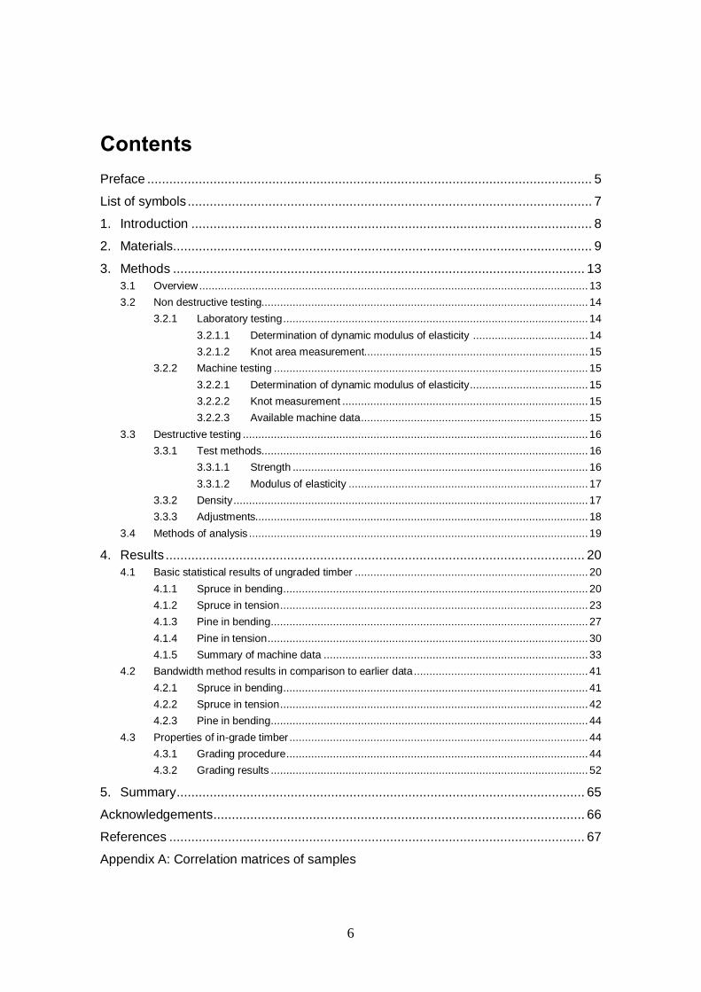
Table 1. Number of tested specimens split into source country, region, species and test mode.
Source country Region Spruce Pine
Total bending tension bending tension
CH Jura 0 146 0 0 146 Mittelland 0 148 0 0 148 Voralpen/Alpen 0 148 0 0 148
FI East 0 0 0 172 172 West 0 0 0 85 85
FR Auvergne ,-600 m 0 0 0 118 118 Auvergne +600 m 0 0 0 121 121 Alsace 103 0 0 0 103 Lorraine 12 0 0 0 12
PL Murow 214 111 108 107 540 Swietjano 219 108 111 110 548
RO Bucovina_1 114 112 0 0 226 Bucovina_2 88 88 0 0 176 Transylvania 116 113 0 0 229
RU Novgorod 0 0 0 87 87 Vologda 0 0 0 84 84
SE Gästrikland 0 0 0 35 35 Lappland 105 111 34 35 285 Västerbotten 0 0 35 34 69 Västergötland 105 100 140 102 447
SI Central Slovenia 489 0 0 0 489 Inner Carniola 218 0 0 0 218 Slovenian Carinthia 314 0 0 0 314 Upper Carniola 104 104 0 0 208
SK Prešov 107 112 0 0 219 Žilina 100 99 0 0 199
UA Iwano-Frankiwsk_1 134 133 0 0 267 Iwano-Frankiwsk_2 69 70 0 0 139 Lemberg 112 117 0 0 229
Total 2 723 1 820 428 1 090 6 061
The seven participating laboratories were responsible for sampling. Depending on the source country and the expertise of the research laboratories it was tried to identify the source of the timber as precise as possible. Most specimens were ordered in three dif-ferent cross-sections in order to account for possible size effects: 38 x 100 mm²,

2. Materials
12
50 x 150 mm² and 44 x 200 mm². Independent of the cross-section a length of 4 meters was aspired. Actually sampled dimensions are visualized in Figure 2, not considering the width of 74 pieces with a specialized cross-section of 140 x 140 mm2 from Slovenia in the diagram for thickness. While for thickness and width no differences based on the origin were found, the timber from FI, SE and RU clearly differs from the aspired length.
Figure 2. Dimensions of the sampled material.

3. Methods
13
3. Methods
3.1 Overview
Prior to testing each specimen destructively, nondestructive measurements have been performed by participating laboratories as well as by participating grading machine pro-ducers. All measurements are listed in Table 2. A description of methods and calcula-tion of the numerical results is given method by method in the following.
Table 2. Measured property by participants.
Participant (equipment) Measured property
all laboratories frequency width, thickness. length weight moisture content KAR, KAR position local, global modulus of elasticity maximum force destructive test time strength ETH, FCBA, TUM, UL running time Rosegrade frequency Escan, MTG frequency density Triomatic running time local density GoldenEye-706, Combiscan frequency density knots

3. Methods
14
3.2 Non destructive testing
3.2.1 Laboratory testing
3.2.1.1 Determination of dynamic modulus of elasticity
The dynamic modulus of elasticity was determined based on weight, length, width and thickness as well as on the frequency of longitudinal vibration. In addition some research partners quantified the dynamic modulus of elasticity by means of ultrasonic waves.
Width and thickness were measured at different points over the length. The mean val-ue of the measurements was reported. Measuring the length with a tape and the weight of the timber using a scale allowed to calculation the global density of the board. Ob-tained density is called specimen here.
Moisture content measurements are necessary to get comparable modulus of elasticity at a moisture content of 12%, as parameters alter depending on it. Depending on the time difference between measuring the variables for the calculation of the dynamic MOE and the destructive tests, the moisture content has been determined based on the difference between the mass before drying (mu) and after drying (m0) (EN 13183-1) of a defect free piece of timber or based on the electric resistance method.
For the natural frequency measurement the first resonance frequency in longitudinal vibration was determined. The measurement in laboratory was done by placing each specimen on two elastic supports and hitting one end of it by a hammer, or something similar, which excites the vibration. The vibration was measured in several different ways (microphone, accelerometer, optically). Based on the natural frequency and length measurement only, the dynamic modulus of elasticity can not be calculated. Still the two variables were used to calculate Efreq,test, which lets us estimate the dynamic MOE. This was done, as Efreq,test comes close to IPs from grading machines which measure the frequency but not the density. As for laboratory measurements density is available, a real dynamic modulus of elasticity value is obtained (Edyn,test). Obviously the accuracy in prediction static modulus of elasticity and density for the one including information about density is higher than the one without it. The two modulus of elasticity values are calculated as follows:
4502
, 2 LfreqE testfreq (1)
testspecimentestdyn LfreqE ,2
, 2 (2)
where 450 is assumed constant value of density (450 kg/m3) and specimen,test is based on measurement of each specimen. These dynamic modulus of elasticity values are adjust-ed to 12% moisture content similarly as static modulus of elasticity in Equation (7).

3. Methods
15
The dynamic modulus of elasticity by use of sound waves was additionally calculated, if an ultrasonic device was available at a laboratory. Therefore, the running time of the waves was measured by attaching two probes on the ends of the specimen. An ultrasonic sound pulse is excited to the specimen at one end. At the other end the transit time and transmitted energy is measured.
3.2.1.2 Knot area measurement
The knot area ratio (KAR) is the ratio of the area of the knots projected on a cross sec-tion to the cross sectional area of the piece. Overlapping knot areas were counted only once. The KAR knot cluster was detected over a length of 150 mm. If the board con-tains pith, the exact position was determined in order to design the knot areas. The KAR value was determined in the relevant testing range only. This means, that for bending tests the range is limited to the distance between the inner load points plus one times the width on the right and the left border. For tension testing the knots were detected on the whole length between the two jaws.
3.2.2 Machine testing
3.2.2.1 Determination of dynamic modulus of elasticity
All machine producers use frequency or running time measurements for predicting tim-ber properties. Main difference is on the measurement device for the frequency and the density measurements. While most machines use scales for calculating the density, one machine uses x-ray radiation for getting a density value. One machine does not measure density at all.
3.2.2.2 Knot measurement
Knot measurements are done by Luxscan and MiCROTEC. Luxscan uses optical knot detection software for calculating knot values, while MiCROTEC uses x-ray radiation. Both manufacturers calculate different knot values to be able to get the best predicting value for different species.
3.2.2.3 Available machine data
Based on the machine measurement, up to three IPs are calculated for each machine. Not every piece was measured by each machine system, as some manufacturers did not grade all specimens (Table 3). Even if manufacturers graded all specimens, the number

3. Methods
16
of available IPs can deviate from the maximum possible number, if necessary infor-mation was not recorded by the system.
Table 3. Numbers of specimens which were measured by different machine systems.
Machine & Indicated property Pine Spruce
bending tension bending tension
GoldenEye-706, Indicating strength 428 1 090 2 723 1 820
GoldenEye-706, Indicating stiffness 428 1 090 2 723 1 820
GoldenEye-706, Indicating density 428 1 090 2 723 1 820
Combiscan, Indicating strength 428 1 053 2 646 1 377
Escan, Indicating strength 428 1 053 2 646 1 377
Escan, Indicating density 428 1 053 2 646 1 377
Triomatic, Indicating strength 427 1 041 2 704 1 808
Triomatic, Indicating density 427 0 2 274 1 590
Rosegrade, Indicating strength 423 1 069 2 705 1 805
MTG, Indicating strength 418 1 073 2 671 1 761
MTG, Indicating stiffness 418 1 073 2 671 1 761
MTG, Indicating density 418 1 073 2 671 1 761
3.3 Destructive testing
3.3.1 Test methods
3.3.1.1 Strength
Destructive tests have been preformed according to EN 408 and calculated to reference values following mainly EN 384.
The critical cross section was chosen visually and placed between the loading heads in bending or between the jaws in tension. Following EN 384, only the critical cross section that can be located between the loading heads in a bending test or between the jaws in a tension test was considered.

3. Methods
17
Bending tests were performed using a distance between the supports of 18*width of the specimen and a distance between loading heads was 6*width. The load was applied on the edge of the specimen and the tension edge was selected at random.
In tension the critical cross section was located in the range of 9*width. The speci-mens were gripped by jaws on both endings. The length of gripping was between 800 mm and 1 200 mm on each side.
For some measurements this general set up was not followed: ETH performed tension tests over the maximum possible free test length exceeding 3 000 mm. HFA had to de-crease the distance of the supports for some specimens with a width of 220 mm in bend-ing, as these specimens were too short. In this case, the total test length was 16 times the width, the distance of the inner load points was 6 times the width.
3.3.1.2 Modulus of elasticity
Both, static local and static global moduli of elasticity were measured for bending. Ex-cept for ETH, which used a different test setup, one modulus of elasticity value was delivered for tension.
The static local modulus of elasticity in edgewise bending and the static local modu-lus of elasticity in tension are determined in accordance to EN 408, i.e. that the gauge length for the determination of the modulus of elasticity is 5 times the width. If possible, modulus of elasticity was determined in the linear range of the stress-strain diagram between 10% and 40% of the maximum stress.
For some measurements these instructions were not followed. ETH chose a different test setup for the tension tests using the whole length of each specimen. For that reason they had more freedom to choose the position for the static local modulus of elasticity measurement. If possible this was done at the position of the biggest KAR value. Addi-tionally, values for a global modulus of elasticity calculated from the tension test ma-chine were transmitted. UL measured the displacement for the local bending modulus of elasticity on the lower face of the specimens.
3.3.2 Density
The density was measured by taking a section which was cut out of each specimen as close as possible to the fracture. As mentioned in EN 408 the section was of full cross section, free from knots and resin pockets. This section was dried, so that its dry mass, volume and density can be determined. Reported densities based on these small sections are named in the following and were corrected to a moisture content of 12%.

3. Methods
18
3.3.3 Adjustments
To keep laboratory data comparable EN 384 fixes reference values for moisture content, size and test arrangement. These references are...
...moisture content of 12%
...width of 150 mm
...distance between the supports of 18*width in bending
...distance between the loading heads of 6*width in bending
...distance between the jaws of 9*width in tension.
To adjust laboratory data to these references the following equations were used. Most of the equations are given in EN 384. In the case of length adjustment for tension the ex-ponent was taken from EN 1194.
- Adjustment of bending strength to similar size:
for width: testmm fwidthf ,2.0150/ (3)
for length: testmm fwidthaf ,2.048/5 (4)
- Adjustment of tensile strength to similar size:
for width: testtt fwidthf ,2.0150/ (5)
for length: testtt fwidthf ,1.09/ (6)
- Adjustment of modulus of elasticity
to a moisture content u = 12%: )12(01.01/ uEE test (7)
to a pure modulus of elasticity in bending if tested globally:
26903,1 globalEE (8)
In the case of Efreq,test the correction according to SCHNABEL 2006 was used.
- Adjustment of density values to a moisture content u = 12%
)12(005.01/ utest (9)
In the following chapters the authors refer to adjusted values only. Also all regression analysis is based on adjusted values like strength, modulus of elasticity and density.

3. Methods
19
3.4 Methods of analysis
Statistical analysis of the results is made by using standard methods. In addition, “bandwidth” method was used for analysis of similarity of graded timber grown in dif-ferent areas [1].
Strength, stiffness or density indicating properties IP1–IP12 are calculated based on readings of participating grading machines identified in Table 4. These are regression lines between the grade determining property and one or more measured parameters in all data, separately for spruce in bending and tension and for pine in bending and ten-sion. Used IP-functions for MTG machine are based on old data from different growth area which may course lower correlation between IP and grade determining property in our results. These functions of all machines may be different from those used in com-mercial grading.
Table 4. Numbering of machine IP’s.
IP1 GoldenEye-706, Indicating strength
IP2 GoldenEye-706, Indicating stiffness
IP3 GoldenEye-706, Indicating density
IP4 Combiscan, Indicating strength
IP5 Escan, Indicating strength
IP6 Escan, Indicating density
IP7 Triomatic, Indicating strength
IP8 Triomatic, Indicating density
IP9 Rosegrade, Indicating strength
IP10 MTG, Indicating strength
IP11 MTG, Indicating stiffness
IP12 MTG, Indicating density
Regression lines are calculated for the grading machine model (IP1) with highest coef-ficient of determination:
f = a IP1 + b (10)
and for the model equivalent to the most commonly used grading method today: dcEf freq (11)
Obtained values for coefficients a, b, c and d are given in Appendix A in the same tables with correlations, separately for each region.

4. Results
20
4. Results
4.1 Basic statistical results of ungraded timber
4.1.1 Spruce in bending
Summary of destructive test results for spruce in bending are given in Table 5, which shows means and CoV’s of strength, stiffness and density separately for each country and for the combined sample. Same information is given also of existing results from Sweden and Germany as reference of Northern and Central European values. New Swedish sample has on average same density but lower modulus of elasticity and strength than Swedish reference data. Slovenian and French samples have values on the same level as the earlier German data, but all other samples have lower average proper-ties. All mean values of Romanian, Ukraine and Slovakian samples are clearly below Central European reference.
Degrees of determination between destructive and non-destructive test values are shown for combined spruce sample in Table 6. Results for participating grading ma-chines are shown in Table 13. Correlations for each sample are in Appendix A. Also regression lines are calculated for the model (IP1) with highest coefficient of determina-tion, and for the model equivalent to the most commonly used grading method today (Efreq). Obtained values for coefficients a and b of Equation (10), and c and d of Equa-tion (11) are given in Appendix A in the same tables with correlations, separately for each region.
Some regression lines are shown in Figures 3–6. Figures 3 and 5 show regression lines between strength and IP1, and Figures 4 and 6 between strength and Efreq. Varia-tion between regression lines based on IP1 is smaller than between lines based on Efreq. Variation between Slovenian regions is clearly larger in case of Efreq than between all samples from Slovenia, Ukraine, Poland and some others in case of IP1 in Figure 5.
Most different from the others were the sample from Västergötland (highest slope) and Alsace (highest level). Sample of Prešov shows exceptionally high slope in case of Efreq but low slope in case of IP1.

4. Results
21
Table 5. Summary of the destructive test results of spruce in bending. For comparison some results of [1] are also shown.
fm E n
SPRUCE bending mean COV mean COV mean COV
N/mm2 N/mm2 kg/m3
Sweden 42.5 0.35 11 300 0.22 435 0.12 210
Poland 38.5 0.31 11 400 0.20 440 0.11 433
Slovenia 43.7 0.30 12 000 0.20 445 0.10 1 163
France 42.9 0.26 11 900 0.17 440 0.10 118
Slovakia 34.8 0.33 10 200 0.20 415 0.10 213
Romania 35.5 0.31 9 600 0.19 387 0.10 321
Ukraine 36.2 0.29 10 000 0.19 389 0.10 204
All above 40.2 0.32 11 200 0.21 428 0.11 2 776
Sweden, earlier data 44.8 0.30 12 300 0.22 435 0.12 4 393
Germany, earlier data 41.5 0.34 12 100 0.26 441 0.11 3 538
Table 6. Coefficient of determination r2 of individual NDT-measurements to destructively deter-mined properties for spruce in bending.
SPRUCE bending Source
to destruct. r2 of fm Eglobal n
Destructive test fm 1.00 0.66 0.28 2 776
Destructive test Eglobal 0.66 1.00 0.54 2 776
Destructive test 0.28 0.54 1.00 2 776
Lab. weighing by scale specimen 0.25 0.50 0.94 2 776
Lab. NDT/Freq. Efreq 0.51 0.68 0.23 2 776
Lab. NDT/Freq. + dens. Edyn 0.54 0.83 0.66 2 776
Lab. NDT/ultrasonic Edyn(running time) 0.40 0.70 0.66 1 612
Lab. visual KAR 0.31 0.21 0.06 2 776

4. Results
22
Figure 3. Regression lines between bending strength of spruce and IP1 in all regions.
Figure 4. Regression lines between bending strength of spruce and Efreq in all regions.
0
10
20
30
40
50
60
0 10 20 30 40 50 60
f m(N
/mm
2 )
IP1
MurowSwietjanoIwano-FrankiwskUpper CarniolaSlov CarinthiaInner CarniolaCentral SloveniaTransylvaniaBucovina_2Bucovina_1PrešovŽilinaAlsaceLapplandVästergötlandall
0
10
20
30
40
50
60
5 7 9 11 13 15
f m(N
/mm
2 )
Efreq (kN/mm2)
MurowSwietjanoIwano-FrankiwskUpper CarniolaSlov CarinthiaInner CarniolaCentral SloveniaTransylvaniaBucovina_2Bucovina_1PrešovŽilinaAlsaceLapplandVästergötlandall

4. Results
23
Figure 5. Regression lines between bending strength of spruce and IP1 in all regions except Sweden, Alsace, Bucovina and Presow. “All” refers to all tested data.
Figure 6. Regression lines between bending strength of spruce and Efreq in Slovenian regions. “All” refers to all tested data.
4.1.2 Spruce in tension
Summary of destructive test results for spruce in tension are given in Table 7, which shows means and CoV’s of strength, stiffness and density separately for each country and for the combined sample. For reference, earlier results from Finland, Austria and
0
10
20
30
40
50
60
0 10 20 30 40 50 60
f m(N
/mm
2 )
IP1
MurowSwietjanoIwano-FrankiwskUpper CarniolaSlov CarinthiaInner CarniolaCentral SloveniaTransylvaniaŽilinaall
0
10
20
30
40
50
60
5 7 9 11 13 15
f m(N
/mm
2 )
Efreq (kN/mm2)
Upper Carniola
Slov Carinthia
Inner Carniola
Central Slovenia
all
4. Results
24
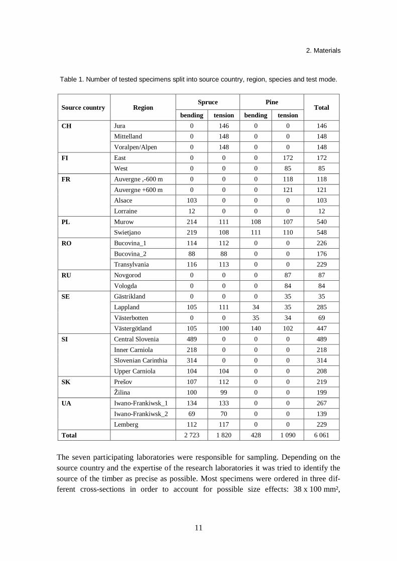
Germany are also given. New results of Slovenia are the highest and compatible to ear-lier sample from Schwaben, Germany. The new sample of Sweden shows low values which are below the earlier data from Finland. The old sample of Austria has the lowest strength, but new samples from Romania and Ukraine have the lowest densities and moduli of elasticity.
Coefficients of determination between destructive and non-destructive test values are shown for combined spruce sample in Table 8. Results for participating grading ma-chines are shown in Table 13. Values are on same level as they were in case of spruce in bending. Correlations for each sample are in Appendix A. Also regression lines are cal-culated for the model (IP1) with highest coefficient of determination and for the model equivalent to the most commonly used grading method today (Efreq).
Obtained values for coefficients a and b of Equation (10), and c and d of Equation (11) are given in Appendix A in the same tables with correlations, separately for each region.
Regression lines of all samples are shown in Figures 7 and 8. Quite similar regression lines can be found in different countries (Figure 9) and some variability within one country (Figure10).
Table 7. Summary of the destructive test results of spruce in tension. For comparison some results of [1] are also shown. Strength values are adjusted to reference width 150 mm and to free length 1 350 mm.
ft E n
SPRUCE tension mean COV mean COV mean COV
N/mm2 N/mm2 kg/m3
Sweden 27.6 0.38 10 200 0.23 416 0.12 218
Poland 28.2 0.38 11 600 0.23 452 0.12 222
Slovenia 34.0 0.44 12 300 0.22 442 0.09 104
Switzerland 27.8 0.44 10 900 0.24 439 0.12 447
Slovakia 27.2 0.40 10 700 0.20 408 0.09 215
Romania 25.6 0.42 10 000 0.21 390 0.08 319
Ukraine 26.7 0.44 10 300 0.21 392 0.11 329
All above 27.5 0.43 10 700 0.23 418 0.12 1 854
Finland, earlier data 33.2 0.34 11 800 0.19 445 0.10 611
Austria, earlier data 25.1 0.42 10 100 0.26 435 0.12 311
GER Schwaben, earlier data 32.6 0.37 12 100 0.21 451 0.11 588

4. Results
25
Table 8. Coefficient of determination r2 of individual NDT-measurements and grading machine IP’s to destructively determined properties for spruce in tension. N = 1 854 (883 for “lab NDT/ ultrasonic”).
SPRUCE tension Source to destruct. r2 of
ft E
Destructive test ft 1 0.63 0.21
Destructive test E 0.63 1 0.45
Destructive test 0.21 0.45 1
Lab. weighing by scale specimen 0.17 0.37 0.86
Lab. NDT/Freq. Efreq 0.59 0.65 0.12
Lab. NDT/Freq. + dens. Edyn 0.59 0.83 0.56
Lab. NDT/ultrasonic Edyn(running time) 0.42 0.70 0.66
Lab. visual KAR 0.33 0.22 0.04
Figure 7. Regression lines between tension strength of spruce and IP1 in all regions.
0
10
20
30
40
50
0 10 20 30 40 50
f t(N
/mm
2 )
IP1
LembergTransylvaniaPrešovUpper CarniolaVoralpen/AlpenŽilinaBucovinaallJuraIwano-FrankiwskMurowVästergötlandSwietjanoMittellandLappland

4. Results
26
Figure 8. Regression lines between tension strength of spruce and Efreq in all regions.
Figure 9. Regression lines between tension strength of spruce and IP1 in selected regions of Poland, Switzerland, Slovakia, Slovenia, Romania and Ukraine. “All” refers to all tested data.
0
10
20
30
40
50
6 8 10 12 14 16
f t(N
/mm
2 )
Efreq (kN/mm2)
Upper CarniolaPrešovLembergTransylvaniaVästergötlandJuraMurowŽilinaallBucovinaIwano-FrankiwskMittellandSwietjanoVoralpen/AlpenLappland
0
10
20
30
40
50
0 10 20 30 40 50
f t(N
/mm
2 )
IP1
Prešov
Upper Carniola
Žilina
Bucovina
all
Jura
Iwano-Frankiwsk
Murow

4. Results
27
Figure 10. Regression lines between tension strength of spruce and IP1 in tested regions of Switzerland. “All” refers to all tested data.
4.1.3 Pine in bending
Summary of destructive test results for pine in bending are given in Table 9, which shows means and cov’s of strength, stiffness and density separately for each country and for the combined sample. New results from Sweden are on same level as old results from Finland. New results from Poland are similar to old results from North Germany. There is a clear difference in average properties between North and Central Europe: strength is 10% higher in North, and modulus of elasticity and density are higher in Central Europe. The Nordic values of pine are similar to spruce, except for density: pine has higher density than spruce.
Coefficients of determination between destructive and non-destructive test values are shown for combined pine sample in Table 10. Results for participating grading ma-chines are shown in Table 13. Correlations for each sample are in Appendix A. Espe-cially Swedish samples show higher correlation between strength and some indicating properties (density, KAR) which have low correlation in case of spruce. However, in combined Swedish-Polish sample, we cannot see higher correlation with density.
Also regression lines are calculated for the model (IP1) with highest coefficient of de-termination, and for the model equivalent to the most commonly used grading method today (Efreq). Obtained values for coefficients a and b of Equation (10), and c and d of Equation (11) are given in Appendix A in the same tables with correlations, separately for each region.
0
10
20
30
40
50
0 10 20 30 40 50
f t(N
/mm
2 )
IP1
Voralpen/Alpen
all
Jura
Mittelland

4. Results
28
Regression lines of all samples are shown in Figures 11 and 12. In case of Efreq as in-dicating property one of the Swedish samples (Västerbotten) has regression line on 10 N/mm2 higher level. In mean values, difference is nearly 20 N/mm2. When looking at numerical values of Efreq one should notice that it is calculated on basis of assumed den-sity = 450 kg/m3 which is low value for pine and gives about 10% lower values than Edyn based on measured density.
Table 9. Summary of the destructive test results of pine in bending. For comparison some re-sults of [1] are also shown.
fm E n
PINE bending mean COV mean COV mean COV
N/mm2 N/mm2 kg/m3
Sweden 44.7 0.34 11 300 0.19 481 0.09 209
Poland 39.2 0.43 12 500 0.23 516 0.10 221
All above 41.9 0.39 11 900 0.22 499 0.11 430
North Germany, earlier 38.6 0.31 12 200 0.21 522 0.12 421
Finland, earlier data 44.9 0.31 11 900 0.24 493 0.11 849
Table 10. Coefficient of determination r2 of individual NDT-measurements and grading machine IP’s to destructively determined properties for pine in bending, n = 430 (220 for “lab NDT/ ultra-sonic”).
PINE bending Source to destruct. r2 of
fm Eglobal
Destructive test fm 1 0.53 0.21
Destructive test Eglobal 0.53 1 0.54
Destructive test 0.21 0.54 1
Lab. weighing by scale specimen 0.21 0.57 0.89
Lab. NDT/Freq. Efreq 0.46 0.60 0.14
Lab. NDT/Freq. + dens. Edyn 0.50 0.85 0.54
Lab. NDT/ultrasonic1 Edyn(running time) 0.44 0.75 0.54
Lab. visual KAR 0.40 0.25 0.09

4. Results
29
Figure 11. Regression lines between bending strength of pine and IP1 in all regions.
Figure 12. Regression lines between bending strength of pine and Efreq ( = 450 kg/m3) in all regions.
0
10
20
30
40
50
60
0 10 20 30 40 50 60
f m(N
/mm
2 )
IP1
all
Murow
Swietjano
Lappland
Västerbotten
Västergötland
0
10
20
30
40
50
60
5 7 9 11 13
f m(N
/mm
2 )
Efreq (kN/mm2)
all
Murow
Swietjano
Lappland
Västerbotten
Västergötland
4. Results
30
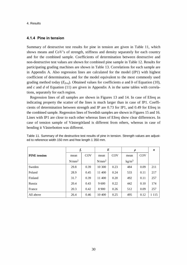
4.1.4 Pine in tension
Summary of destructive test results for pine in tension are given in Table 11, which shows means and CoV’s of strength, stiffness and density separately for each country and for the combined sample. Coefficients of determination between destructive and non-destructive test values are shown for combined pine sample in Table 12. Results for participating grading machines are shown in Table 13. Correlations for each sample are in Appendix A. Also regression lines are calculated for the model (IP1) with highest coefficient of determination, and for the model equivalent to the most commonly used grading method today (Efreq). Obtained values for coefficients a and b of Equation (10), and c and d of Equation (11) are given in Appendix A in the same tables with correla-tions, separately for each region.
Regression lines of all samples are shown in Figures 13 and 14. In case of Efreq as indicating property the scatter of the lines is much larger than in case of IP1. Coeffi-cients of determination between strength and IP are 0.73 for IP1, and 0.49 for Efreq in the combined sample. Regression lines of Swedish samples are shown in Figures 15 and 16. Lines with IP1 are close to each other whereas lines of Efreq show clear differences. In case of tension sample of Västergötland is different from others, whereas in case of bending it Västerbotten was different.
Table 11. Summary of the destructive test results of pine in tension. Strength values are adjust-ed to reference width 150 mm and free length 1 350 mm.
ft E n
PINE tension mean COV mean COV mean COV
N/mm2 N/mm2 kg/m3
Sweden 29.8 0.39 10 300 0.23 484 0.09 211
Poland 28.9 0.45 11 400 0.24 533 0.11 217
Finland 31.7 0.39 11 400 0.20 492 0.11 257
Russia 20.4 0.43 9 600 0.22 442 0.10 174
France 20.3 0.42 8 900 0.26 512 0.09 257
All above 26.4 0.46 10 400 0.25 495 0.12 1 115

4. Results
31
Table 12. Coefficient of determination r2 of individual NDT-measurements and grading machine IP’s to destructively determined properties for pine in tension. N = 1 115 (667 for “lab NDT/ ul-trasonic”).
PINE tension Source to destruct. r2 of
ft E
Destructive test ft 1 0.66 0.27
Destructive test E 0.66 1 0.35
Destructive test 0.27 0.35 1
Lab. weighing by scale specimen 0.22 0.28 0.82
Lab. NDT/Freq. Efreq 0.50 0.62 0.06
Lab. NDT/Freq. + dens. Edyn 0.64 0.79 0.41
Lab. NDT/ultrasonic Edyn(running time) 0.46 0.57 0.21
Lab. visual KAR 0.43 0.30 0.11
Figure 13. Regression lines between tension strength of pine and IP1 in all regions.
0
10
20
30
40
50
0 10 20 30 40 50
f t(N
/mm
2 )
IP1
allFI EastFI WestFR-600 mMurowSwietjanoNovgorodVologdaGästriklandLapplandVästerbottenVästergötlandFR+600 m

4. Results
32
Figure 14. Regression lines between tension strength of pine and Efreq ( = 450 kg/m3) in all regions.
Figure 15. Regression lines between tension strength of pine and IP1 in Swedish regions. “All” refers to all tested data.
0
10
20
30
40
50
5 7 9 11 13 15
f t(N
/mm
2 )
Efreq (kN/mm2)
allFI EastFI WestFR-600 mMurowSwietjanoNovgorodVologdaGästriklandLapplandVästerbottenVästergötlandFR+600
0
10
20
30
40
50
0 10 20 30 40 50
f t(N
/mm
2 )
IP1
all
Gästrikland
Lappland
Västerbotten
Västergötland

4. Results
33
Figure 16. Regression lines between tension strength of pine and Efreq ( = 450 kg/m3) in Swe-dish regions. “All” refers to all tested data.
4.1.5 Summary of machine data
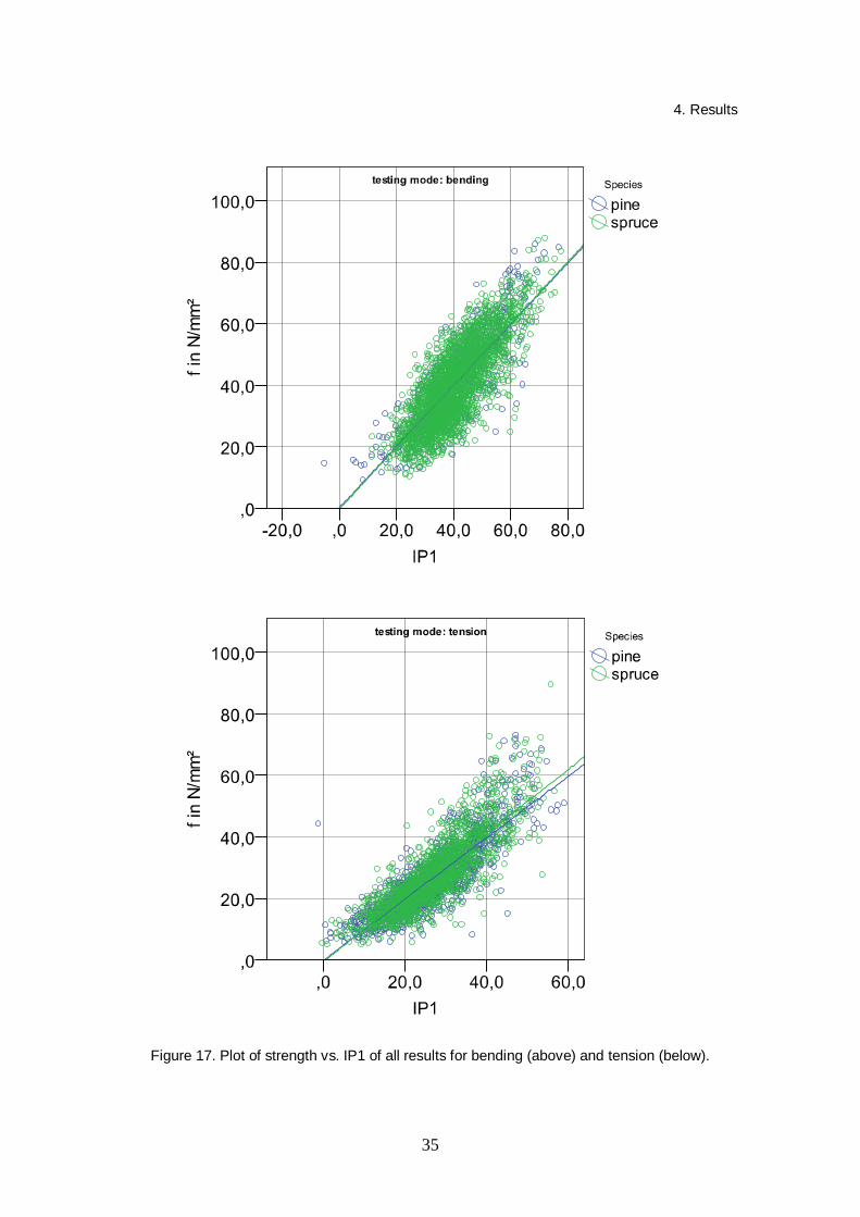
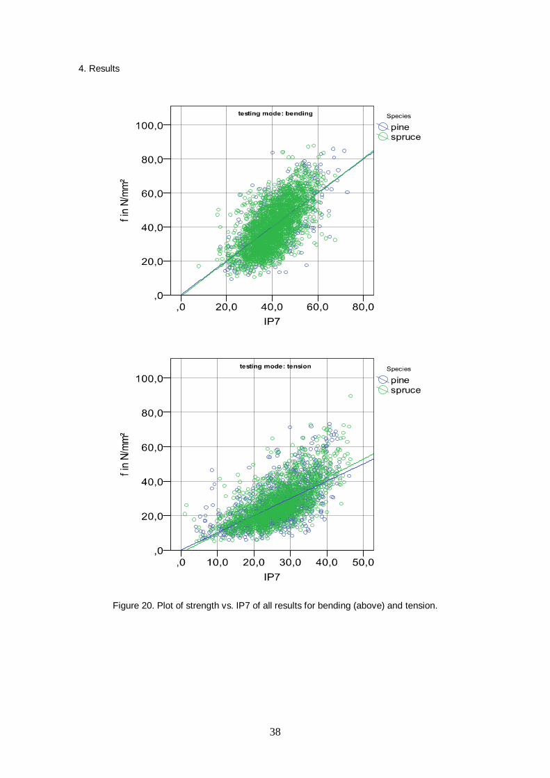
Basical statistic figures for the used grading systems are already considered above. In the following the results are illustrated in Figures 17–22. While the results so far where shown separate for each load mode and species, different species are handeld together in this part. Table 13 summarizes the coefficients of determination.
0
10
20
30
40
50
5 7 9 11 13 15
f t(N
/mm
2 )
Efreq (kN/mm2)
all
Gästrikland
Lappland
Västerbotten
Västergötland

4. Results
34
Table 13. Summary of coefficients of determination r2 of grading machine IP’s to destructively determined properties.
IP Species f in N/mm² E in N/mm² density in kg/m³
bending tension bending tension bending tension
IP1 pine 0,67 0,72 0,68 0,74 0,34 0,35
spruce 0,63 0,70 0,82 0,77 0,51 0,31
IP2 pine 0,52 0,64 0,84 0,78 0,50 0,43
spruce 0,55 0,58 0,86 0,84 0,66 0,61
IP3 pine 0,28 0,25 0,61 0,29 0,86 0,84
spruce 0,28 0,20 0,54 0,43 0,93 0,89
IP4 pine 0,56 0,62 0,64 0,72 0,36 0,42
spruce 0,54 0,58 0,79 0,80 0,50 0,52
IP5 pine 0,39 0,57 0,75 0,76 0,50 0,42
spruce 0,50 0,53 0,81 0,82 0,56 0,58
IP6 pine 0,17 0,25 0,45 0,31 0,70 0,76
spruce 0,20 0,15 0,41 0,36 0,69 0,72
IP7 pine 0,43 0,39 0,63 0,50 0,31 0,05
spruce 0,41 0,46 0,64 0,57 0,24 0,14
IP8 pine 0,42 - 0,63 - 0,36 -
spruce 0,35 0,38 0,60 0,59 0,41 0,50
IP9 pine 0,41 0,50 0,59 0,63 0,16 0,06
spruce 0,47 0,58 0,66 0,65 0,18 0,12
IP10 pine 0,48 0,59 0,83 0,76 0,57 0,51
spruce 0,46 0,50 0,72 0,74 0,58 0,48
IP11 pine 0,51 0,58 0,83 0,75 0,50 0,35
spruce 0,47 0,53 0,73 0,75 0,56 0,47
IP12 pine 0,16 0,09 0,46 0,12 0,78 0,68
spruce 0,19 0,11 0,38 0,29 0,71 0,62
4. Results
35
Figure 17. Plot of strength vs. IP1 of all results for bending (above) and tension (below).

4. Results
36
Figure 18. Plot of strength vs. IP4 of all results for bending (above) and tension.

4. Results
37
Figure 19. Plot of strength vs. IP5 of all results for bending (above) and tension.
4. Results
38
Figure 20. Plot of strength vs. IP7 of all results for bending (above) and tension.

4. Results
39
Figure 21. Plot of strength vs. IP9 of all results for bending (above) and tension.

4. Results
40
Figure 22. Plot of strength vs. IP10 of all results for bending (above) and tension.

4. Results
41
4.2 Bandwidth method results in comparison to earlier data
The previous existing data of spruce in bending and tension as well as pine in bending has been analysed by the use of bandwidth method [1]. Comparison was made by divid-ing the data into bands of indicating properties (several different functions) and calcula-tion of characteristic strength values (incl. confidence intervals) for these bands of mate-rial from different growth regions. This information was planned to be used for deter-mination of grading areas where same settings could be used.
New tested material is now added to some Figures of [1] and comparison is made be-tween new and old sampling regions. Model 2 of [1] (strength IP based of Edyn) is used here which is regression line of the old data. Coefficients of equations are given in Ta-bles 34, 41 and 49 of an earlier publication [1]. Confidence interval calculation of 5th percentile values is also explained in [1]. In brief, = 3 limit means 90% confidence interval in case of Normal distribution and 99% interval in case of lognormal distribu-tion. The 5th percentile is calculated based on Normal distribution without any sample size dependent factor.
4.2.1 Spruce in bending
New data of Poland, Slovakia, Slovenia, Romania and Ukraine is combined with the existing data of Germany, France and Slovenia in Figure 23. Model 2 equation used for spruce in bending is
51.000337.0mod dynel Ef (12)
Bandwidths corresponding roughly grade combination C35-C30-C20-C14 are shown. All new results are within confidence limits except the Romanian sample which is above in one band. Old Slovenian values are clearly below as shown already in [1]. Old North German values are below in two bands.

4. Results
42
Figure 23. Characteristic bending strength vs. IP(Edyn) of Central and Eastern European spruce. Abbreviations of countries with three characters refer to old data [1] and two letter abbreviations to new test data.
4.2.2 Spruce in tension
New data of Switzerland, Poland, Slovakia, Slovenia, Romania and Ukraine is com-bined with the existing data of Germany, Austria and Czech Republic in Figure 24. Model 2 equation used for spruce in tension is
82.1600337.0mod dynel Ef (13)
Bandwidths corresponding roughly grade combination T26-T20-T17-T10 are used. The figure is shown in form of strength vs. Edyn. Nearly all new and old results are within confidence interval.
New data from Sweden has been combined with the existing data from Finland and North West Russia. Same strength model (13) has been used and results are shown in Figure 25. None of the values is below the lower confidence limit.
Tension test specimens of Swizerland, Finland and Russia were longer than standard-length 9h of EN 408 and values are adjusted by the use of Equation (6). This adjustment was not made in former publication [1].
0
5
10
15
20
25
30
35
40
45
50
20 30 40 50 60
Cha
ract
eris
tic s
tren
gth
[N/m
m2 ]
IP(Model 2)
w-mean allupper bound ( =3)lower bound ( =3)GER N N=456GER W N=1337SLO N=293FRA N=643UA N=316SK N=213SI N=1163RO N=321PL N=433

4. Results
43
Figure 24. Characteristic tension strength vs. Edyn of Central and Eastern European spruce.
Figure 25. Characteristic tension strength vs. Edyn of North European spruce. Abbreviations of countries with three characters refer to old data [1] and two letter abbreviations to new test data.
0
5
10
15
20
25
30
35
7000 9000 11000 13000 15000 17000
Char
acte
ristic
str
engt
h [N
/mm
2 ]
Edyn [kN/mm2]
w-mean allupper bound ( =3)lower bound ( =3)GER 3 N=517Schwaben N=588CZ N=373Fügen N=311unknown N=889PL N=219CH N=447UA N=203RO N=203SK N=100SI N=104
0
5
10
15
20
25
30
35
40
45
7000 9000 11000 13000 15000 17000
Char
acte
ristic
stre
ngth
[N/m
m2 ]
Edyn [kN/mm2]
w-mean all
upper bound ( =3)
lower bound ( =3)
FIN N=270
RUS N=186
SE N=218

4. Results
44
Figure 26. Characteristic bending strength vs. Edyn of Nordic and Polish pine. Abbreviations of countries with three characters refer to old data [1] and two letter abbreviations to new test data.
4.2.3 Pine in bending
Properties of pine are considered in Northern Europe. Finnish and Swedish pines have been found to be very similar [1]. Combination of Finnish, Swedish, North West Rus-sian and Polish data is shown in Figure 26. Bandwidths corresponding roughly to grade combination C40-C30-C22-C16 are shown. Polish values are clearly below confidence interval. Model 2 equation used for pine in bending is
78.1400472.0mod dynel Ef (14)
The figure is shown in form of strength vs. Edyn.
4.3 Properties of in-grade timber
4.3.1 Grading procedure
The aim of this chapter is to evaluate the Gradewood data using machine strength grad-ing and the method given in EN 14081-2. The grading process is simulated in this case as the IP used in this chapter is based on adjusted laboratory data. Errors due to measur-ing uncertainties or errors which will happen during the grading process of a machine
0
10
20
30
40
50
60
8000 10000 12000 14000 16000
Cha
ract
eris
tic s
tren
gth
[N/m
m2 ]
Edyn [N/mm2]
w-mean allupper bound ( =3)lower bound ( =3)FIN W N=181FIN E N=481RUS N=379SWE N=191SE N=210PL N=221

4. Results
45
are not included in that case. As mentioned in chapter 3.3.3 all laboratory data was cor-reted to reference values before using it for the regression analysis.
The dataset is graded based on linear regression models. Two different machine types are simulated: The “type 1” machine can measure longitudinal frequency (f), length (l) and cross section, density ( ) and the total knot area ratio (KAR) of each specimen. The “type 2” machine can measure longitudinal frequency (f) and length of each piece (l).The results of these two machines are compared in the following.
Table 14 summarizes the regression equations separated into species, testing mode and type of machine. For IP the subscript shows the referred characteristic value as an IP can be one for strength, modulus of elasticity or density.
Table 14. Regression equations for the indicating property of strength separated into species, testing mode and machine type.
Species Testing mode Machine type
1 2
based on: frequency length cross section density KAR
based on: frequency length
pine bending IPf = +11,0 +0,00345*Edyn -42,0*KAR
IPf,E,dens = -1750 + 1,1222* Efreq
IPE = Edyn
IPdens = specimen
tension IPf = +0,47 +0,00314* Edyn -34,8*KAR
IPE = Edyn
IPdens = specimen
spruce bending IPf = +12,2 +0,00321* Edyn -36,0*KAR
IPE = Edyn
IPdens = specimen
tension IPf = +0,153 +0,00323* Edyn - 31,2*KAR
IPE = Edyn
IPdens = specimen

4. Results
46
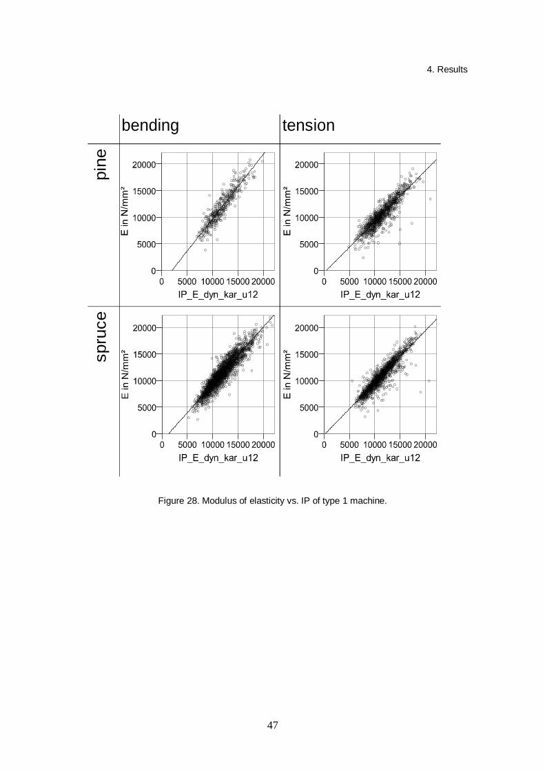
Figure 27 to Figure 29 show the relationship of strength, modulus of elasticity and den-sity versus the IP of machine type 1 divided into testing mode and species. Figure 30 to Figure 32 show the same figures for the IP of machine type 2.
Figure 27. Strength vs. IP of type 1 machine.
bending tension
pine
spru
ce
4. Results
47
Figure 28. Modulus of elasticity vs. IP of type 1 machine.
bending tensionpi
nesp
ruce

4. Results
48
Figure 29. Density vs. IP of type 1 machine.
bending tensionpi
nesp
ruce

4. Results
49
Figure 30. Strength vs. IP of type 2 machine.
bending tensionpi
nesp
ruce

4. Results
50
Figure 31. Modulus of elasticity vs. IP of type 2 machine.
bending tensionpi
nesp
ruce

4. Results
51
Figure 32. Density vs. IP of type 2 machine.
For grading results with respect to EN 14081-2 the authors focused on spruce in bend-ing. As machine type 2 is based on Efreq only, the machine is not possible to use more than one IP to grade the material. To be able to directly compare the results of machine type 2 to the results of machine type 1 only the IP based on strength (IPf in Table 14) was used for grading the material with machine type 1.
Following EN 14081-2 the settings are calculated for sub-samples based on countries. These settings are used to show differences between countries, regions and within sawmills. To keep results comparable the following grading combinations are used: C35 / C24 / Rej, C30 / C18 / Rej and C24 / Rej. Table 15 summarizes the information of grading procedure.
bending tensionpi
nesp
ruce

4. Results
52
Table 15. Summary of grading procedure, IPs and settings.
Species Spruce
Load mode Bending
settings calculated following to EN 14081-2, country
Machine type 1 2
IP & settings used IPf = +12,2 +0,00321* Edyn -36,0*KAR
IPf,E,dens = -1750 + 1,1222* Efreq
C24 / reject 21,3 / 0 8 900
C30 / C18 / reject 36,6 / 18,0/ 0 12 400 / 7 300 / 0
C35 / C24 / reject 46,3 /29,3 / 0 13 600 / 9 400 / 0
4.3.2 Grading results
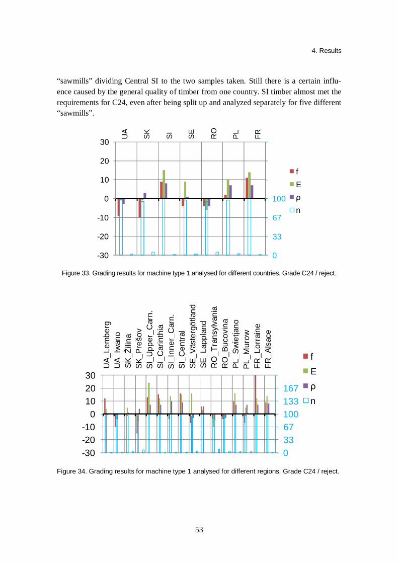
In the following, results were analysed graphically starting with machine type 1 and strength class C24 / reject. Figure 33 shows the results. The first four columns within each country belongs to the highest grade, the following four to the following grade, in our case to the reject grade. The blue columns show the yield, separate into the different source countries, and belong to the right hand ordinate which shows the percentage. For C24 the yield for timber from FR is close to 100 % while the reject is close to 0 %. The red, green and purple columns compare the actually reached values for the strength de-termining properties to the required values for each strength class. The left hand ordi-nate shows these readings in percentage. For strength the requirements are not met for four out of seven countries. Strength values for FR are more than 10% higher than the required value, for SK the opposite is the case. While the strength values can be 10 % lower for single source countries, the characteristic values for stiffness and density seem to be unproblematic.
Increasing the zoom level from countries to regions results in bigger deviations from the required characteristic values. Figure 34 additionally shows that the analysis on country level is not enough. While the grading results from RO are similar for timber from Transylvania and Bucovina and therefore, also to country wise analysis shown in Figure 33, this is not the case for other origins. E.g. for SE, PL or FR there are differ-ences if the data is analysed based on regions. Even the ratio between different grade determining properties can vary significantly. Timber from Västergötland has much higher stiffness values in grade C24 than timber from Lapland in this case.
An analysis on an even smaller level revealed no major surprises (Figure 35). Sam-ples were taken from the same sawmill at different times. In this case, SI, RO and UA can be compared. As SI is a very small country, all "regions" have been included also as
4. Results
53
“sawmills” dividing Central SI to the two samples taken. Still there is a certain influ-ence caused by the general quality of timber from one country. SI timber almost met the requirements for C24, even after being split up and analyzed separately for five different “sawmills”.
Figure 33. Grading results for machine type 1 analysed for different countries. Grade C24 / reject.
Figure 34. Grading results for machine type 1 analysed for different regions. Grade C24 / reject.
0
33
67
100
133
167
200
-30
-20
-10
0
10
20
30
UA
UA
SK SK SI SI SE SE RO
RO
PL PL FR FR
fE
n
UA
SK SI SE RO
PL FR
03367100133167200
-30-20-10
0102030
UA_
Lem
berg
UA_
Iwan
oSK
_Žilin
aSK
_Pre
šov
SI_U
pper
_Car
n.SI
_Car
inth
iaSI
_Inn
er_C
arn.
SI_C
entra
lSE
_Väs
terg
ötla
ndSE
_Lap
plan
dR
O_T
rans
ylva
nia
RO
_Buc
ovin
aPL
_Sw
ietja
noPL
_Mur
owFR
_Lor
rain
eFR
_Als
ace
fE
n

4. Results
54
Figure 35. Grading results for machine type 1 analysed for different sawmills. Grade C24 / reject.
If timber is not only graded into one strength class in one pass, conclusions are differ-ent. The strength class combination C30 / C18 / reject (Figures 36 and 37) and C35 / C24 / reject (Figures 38 and 39) are analysed in the following. Still, the analysis is based on machine type 1 starting with the different countries. Figure 36 shows 8 columns for each country: the first 4 columns show the result for strength class C30 (column for f, E , and n), the following 4 columns the result for strength class C18.
Although strength values for FR are always far above the requirement for C24 graded on its own, the strength value for C18 in the strength class combination C30 / C18 / reject and the strength values for C35 in combination C35 / C24 / reject are not met. A different effect is achieved for timber from Eastern Europe. For grade com-bination C35 / C24 / reject the requirements now are fulfilled in some grades. For both grade combinations, the yield in the highest strength class is clearly lower for the East-ern European countries compared to SI, SE or France. The low yield in the highest strength class and increasing reject amount are connected to a safe grading for timber from Eastern Europe. This statement is only correct as long as machine type 1 is used.
0
33
67
100
133
167
200
-30
-20
-10
0
10
20
30
UA_
Iwan
o_2
UA_
Iwan
o_2
UA_
Iwan
o_1
UA_
Iwan
o_1
SI_U
pper
_Car
n.SI
_Upp
er_C
arn.
SI_C
arin
thia
SI_C
arin
thia
SI_I
nner
_Car
n.SI
_Inn
er_C
arn.
SI_C
entra
l_2
SI_C
entra
l_2
SI_C
entra
l_1
SI_C
entra
l_1
RO
_Buc
ovin
a_2
RO
_Buc
ovin
a_2
RO
_Buc
ovin
a_1
RO
_Buc
ovin
a_1
fE
n
UA_
Iwan
o_2
UA_
Iwan
o_1
SI_U
pper
_Car
n.
SI_C
arin
thia
SI_I
nner
_Car
n.
SI_C
entra
l_2
SI_C
entra
l_1
RO
_Buc
ovin
a_2
RO
_Bus
ovin
a_1

4. Results
55
Figure 36. Grading results for machine type 1 analysed for different countries. Grade C30 / C18 / reject.
Figure 37. Grading results for machine type 1 analysed for different regions. Grade C30 / C18 / reject.
0
33
67
100
133
167
200
-30
-20
-10
0
10
20
30
UA
UA
SK SI SI SE RO
RO
PL FR FR
fE
n
UA
SK SI SE RO
PL FR
03367100133167200
-30-20-10
0102030
UA_
Lem
berg
UA_
Iwan
oSK
_Žilin
aSK
_Pre
šov
SI_U
pper
_Car
n.SI
_Car
inth
iaSI
_Inn
er_C
arn.
SI_C
entra
lSE
_Väs
terg
ötla
ndSE
_Lap
plan
dR
O_T
rans
ylva
nia
RO
_Buc
ovin
aPL
_Sw
ietja
noPL
_Mur
owFR
_Lor
rain
eFR
_Als
ace
fE
n

4. Results
56
Figure 38. Grading results for machine type 1 analysed for different countries. Grade C35 / C24 / reject.
Figure 39. Grading results for machine type 1 analysed for different regions. Grade C35 / C24 / reject.
0
33
67
100
133
167
200
-30
-20
-10
0
10
20
30U
A
UA
SK SI SI SE RO
RO
PL FR FR
fE
n
UA
SK SI SE RO
PL FR
03367100133167200
-30-20-10
0102030
UA_
Lem
berg
UA_
Iwan
oSK
_Žilin
aSK
_Pre
šov
SI_U
pper
_Car
n.SI
_Car
inth
iaSI
_Inn
er_C
arn.
SI_C
entra
lSE
_Väs
terg
ötla
ndSE
_Lap
plan
dR
O_T
rans
ylva
nia
RO
_Buc
ovin
aPL
_Sw
ietja
noPL
_Mur
owFR
_Lor
rain
eFR
_Als
ace
fE
n

4. Results
57
For machine “type 2” the equivalent diagrams are
- strength class combination C24 / reject, Figure 40 country, Figure 41 regions - strength class combination C30 / C18 / reject, Figure 42 country, Figure 43 regions - strength class combination C35 / C24 / reject, Figure 44 country, Figure 45 regions.
Comparing the figures analysed for countries of machine type 1 and machine type 2 (Figure 33 with Figure 40, Figure 36 with Figure 42 and Figure 38 with Figure 44) a considerable larger scatter of the different columns representing the characteristic values can be found. Obviously, the yield in the highest strength class in each combination drops. This is an effect of the lower coefficient of determination of machine type 2 IP compared to machine type 1 IP. This can lead to different effects depending on the source country. Compared to a grading procedure carried out with machine type 1 for strength class combination C35 / C24 / reject, characteristic values for UA are no longer met. On the other hand, the drop in yield leads to safe grading results for French timber in strength class combination C30/ C18 / reject as well as strength class combination C35/ C24 / reject.

4. Results
58
Figure 40. Grading results for machine type 2 analysed for different countries. Grade C24 / reject.
Figure 41. Grading results for machine type 2 analysed for different regions. Grade C24 / reject.
0
33
67
100
133
167
200
-30
-20
-10
0
10
20
30
UA
UA
SK SK SI SI SE SE RO
RO
PL PL FR FR
fE
n
UA
SK SI SE RO
PL FR
03367100133167200
-30-20-10
0102030
UA_
Lem
berg
UA_
Iwan
oSK
_Žilin
aSK
_Pre
šov
SI_U
pper
_Car
n.SI
_Car
inth
iaSI
_Inn
er_C
arn.
SI_C
entra
lSE
_Väs
terg
ötla
ndSE
_Lap
plan
dR
O_T
rans
ylva
nia
RO
_Buc
ovin
aPL
_Sw
ietja
noPL
_Mur
owFR
_Lor
rain
eFR
_Als
ace
fE
n

4. Results
59
Figure 42. Grading results for machine type 2 analysed for different countries. Grade C30 / C18 / reject.
Figure 43. Grading results for machine type 2 analysed for different regions. Grade C30 / C18 / reject.
0
33
67
100
133
167
200
-30
-20
-10
0
10
20
30
UA
UA
SK SI SI SE RO
RO
PL FR
fE
n
UA
SK SI SE RO
PL FR
03367100133167200
-30-20-10
0102030
UA
_Lem
berg
UA_
Iwan
oSK
_Žilin
aSK
_Pre
šov
SI_U
pper
_Car
n.SI
_Car
inth
iaSI
_Inn
er_C
arn.
SI_C
entra
lS
E_Vä
ster
götla
ndSE
_Lap
plan
dR
O_T
rans
ylva
nia
RO
_Buc
ovin
aPL
_Sw
ietja
noPL
_Mur
owFR
_Lor
rain
eFR
_Als
ace
fE
n

4. Results
60
Figure 44. Grading results for machine type 2 analysed for different countries. Grade C35 / C24 / reject.
Figure 45. Grading results for machine type 2 analysed for different regions. Grade C35 / C24 / reject.
0
33
67
100
133
167
200
-30
-20
-10
0
10
20
30
UA
UA
SK SI SI SE RO
RO
PL FR FR
fE
n
UA
SK SI SE RO
PL FR
03367100133167200
-30-20-10
0102030
UA_
Lem
berg
UA_
Iwan
oSK
_Žilin
aSK
_Pre
šov
SI_U
pper
_Car
n.SI
_Car
inth
iaSI
_Inn
er_C
arn.
SI_C
entra
lSE
_Väs
terg
ötla
ndSE
_Lap
plan
dR
O_T
rans
ylva
nia
RO
_Buc
ovin
aPL
_Sw
ietja
noPL
_Mur
owFR
_Lor
rain
eFR
_Als
ace
fE
n

4. Results
61
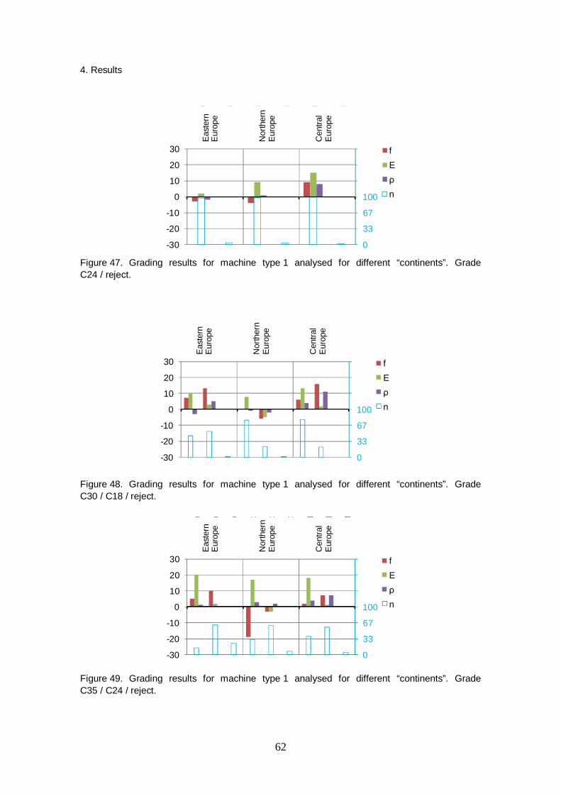
This chapter clearly shows that there are big differences on country level as well as on region and sawmill level. Therefore, segmentation in different countries does not seem to fit. As wood industry is looking for big grading areas to optimise its trading business, one can assume to separate three main grading areas for spruce in bending in Europe. Figure 46 shows this proposal in different colors, Figure 47 to Figure 49 show the results for machine type 1 and the already chosen grade combinations, Figure 50 to Figure 52 show the results for machine type 2, respectively.
Figure 46. Europe divided into Northern Europe, Eastern Europe and Central Europe for spruce in bending.
The already mentioned differences between the three grading areas for spruce in bend-ing can clearly be seen in Figure 47. Also the drop in yield comparing machine type 1 to machine type 2 and the drop in yield in the highest strength classes for Eastern Europe is emphasised in these graphs.
4. Results
62
Figure 47. Grading results for machine type 1 analysed for different “continents”. Grade C24 / reject.
Figure 48. Grading results for machine type 1 analysed for different “continents”. Grade C30 / C18 / reject.
Figure 49. Grading results for machine type 1 analysed for different “continents”. Grade C35 / C24 / reject.
0
33
67
100
133
167
200
-30
-20
-10
0
10
20
30
Ost
euro
pa
Ost
euro
pa
Nor
deur
opa
Nor
deur
opa
Mitt
eleu
ropa
Mitt
eleu
ropa
fE
nE
aste
rn
Eur
ope
Nor
ther
n E
urop
e
Cen
tral
Eur
ope
0
33
67
100
133
167
200
-30
-20
-10
0
10
20
30
Ost
euro
pa
Ost
euro
pa
Ost
euro
pa
Nor
deur
opa
Nor
deur
opa
Nor
deur
opa
Mitt
eleu
ropa
Mitt
eleu
ropa
Mitt
eleu
ropa
fE
n
Eas
tern
E
urop
e
Nor
ther
n E
urop
e
Cen
tral
Eur
ope
0
33
67
100
133
167
200
-30
-20
-10
0
10
20
30
Ost
euro
pa
Ost
euro
pa
Ost
euro
pa
Nor
deur
opa
Nor
deur
opa
Nor
deur
opa
Mitt
eleu
ropa
Mitt
eleu
ropa
Mitt
eleu
ropa
fE
n
Eas
tern
E
urop
e
Nor
ther
n E
urop
e
Cen
tral
Eur
ope

4. Results
63
Figure 50. Grading results for machine type 2 analysed for different “continents”. Grade C24 / reject.
Figure 51. Grading results for machine type 2 analysed for different “continents”. Grade C30 / C18 / reject.
Figure 52. Grading results for machine type 2 analysed for different “continents”. Grade C35 / C24 / reject.
0
33
67
100
133
167
200
-30
-20
-10
0
10
20
30
Ost
euro
pa
Ost
euro
pa
Nor
deur
opa
Nor
deur
opa
Mitt
eleu
ropa
Mitt
eleu
ropa
fE
nE
aste
rn
Eur
ope
Nor
ther
n E
urop
e
Cen
tral
Eur
ope
0
33
67
100
133
167
200
-30
-20
-10
0
10
20
30
Ost
euro
pa
Ost
euro
pa
Ost
euro
pa
Nor
deur
opa
Nor
deur
opa
Nor
deur
opa
Mitt
eleu
ropa
Mitt
eleu
ropa
Mitt
eleu
ropa
fE
n
Eas
tern
E
urop
e
Nor
ther
n E
urop
e
Cen
tral
Eur
ope
0
33
67
100
133
167
200
-30
-20
-10
0
10
20
30
Ost
euro
pa
Ost
euro
pa
Ost
euro
pa
Nor
deur
opa
Nor
deur
opa
Nor
deur
opa
Mitt
eleu
ropa
Mitt
eleu
ropa
Mitt
eleu
ropa
fE
n
Eas
tern
E
urop
e
Nor
ther
n E
urop
e
Cen
tral
Eur
ope

1.
64
The determination of suitable grading areas is not an easy task. Probably, these grading areas will differ for species, type of testing (bending or tension) and type of grading machine (accuracy, multiple IPs, …). Even if suitable grading areas are found for all kinds of combinations, these grading areas can still be increased by using the most con-servative settings for all grading areas or by using more than one IP. Additionally, the responsibility for sawmilling industry may be increased by changing the internal quality control system. This can also have an effect on the definition of grading areas. The Gradewood data perform a very good basis for this future task.
4. Results

5. Summary
65
5. Summary
A large European experimental study on strength of timber is documented. Sampling of spruce and pine includes several countries: new information is obtained from Poland, Slovenia, Slovakia, Romania and Ukraine, from where only little data was available earlier. New is also pine in tension data from Nordic region and France, from where spruce has been tested earlier in large amounts. Valuable for coming research is also that samples from same areas can be used for comparison of tension and bending prop-erties. Main part of the 6 000 specimens has been tested by five participating grading machines and in laboratory by non-destructive and destructive means.
Results include characterisation of national samples in terms of mean values and coef-ficients of variation which have been compared to earlier data from Central and North Europe. Comparisons reveal that Swedish samples of spruce have lower mean strength and larger variation than existing Nordic data, and are obviously not representative for spruce grown in Sweden. This kind of conflict with earlier data we do not observe in other cases, partly also due to lack of earlier data.
Correlations between grade determining properties and measured data have been cal-culated including indicating properties based on grading machine measurements. Re-gression lines between strength and two common IP’s have been determined for each sample separately. Significant conclusion is that regression lines of different regions are closer to each other when IP is based on several measurements and has high correlation with strength. When IP is based on frequency measurement only, variability within a country can be large which is in conflict with the principle of having same model and same settings in a country.
Properties of in-grade timber have been studied when grading method is based on EN 14081-2. Results suggest that same settings might be used separately for North, Central and Eastern Europe. Size of relevant “same grading area” depends on species, type of testing (bending or tension), type of grading machine and if single or multiple IP’s have been applied. The process of defining grading areas has just started and is not finished yet.

5. Summary
66
Acknowledgements
Research plan of Gradewood-project was based on a feasibility study made by the Eu-ropean wood industries under the Roadmap 2010 Building With Wood programme, and this project was supported by the industry via CEI-Bois. CEI-Bois was the main indus-trial financier of this project. Besides the Building With Wood programme financing industries the following companies supported one of the research participants: Martins-sons såg, Setra Group, Norra Skogsägarna, SCA, Swedish Forest Industries Federation, Wood Center North (TCN).
The Gradewood-project belongs to the Wood Wisdom.Net-programme and was fund-ed by national technology development bodies: Tekes, Finnish Funding Agency for
Technology and Innovation (Finland), Vinnova (Sweden), Federal Ministry of Educa-tion and Research (Germany), Ministry of Agriculture (France), and Slovenian Research
Agency. The contributions from funding organisations and other support are grateful-ly acknowledged. The authors want to thank the active industrial leadership of the pro-ject and participating grading equipment producers for their valuable contributions.

Acknowledgements
67
References 1. Strength of European timber. Part 1. Analysis of growth areas based on existing test results.
Ed. by Alpo Ranta-Maunus. VTT Publications 706. Espoo, 2009. 105 p. + app. 63 p. http://www.vtt.fi/inf/pdf/publications/2009/P706.pdf.
2. Schnabel, R. Pilotstudie zur Vorsortierung von frischem Schnittholz mittels Schwingungs-messung. Endbericht im Rahmen des BMWA Förderprogrammes PROKIS (P2b). Holzforschung Austria. Wien, 2006. 36 p. (Only available in German)


Appendix A: Correlation matrices of samples
A1
Appendix A: Correlation matrices of samples
A1: Bending of spruce from France, Poland, Romania, Sweden, Slovenia, Slovakia and Ukraine
A2: Tension of spruce from Switzerland, Poland, Romania, Sweden, Slovenia, Slo-vakia and Ukraine
A3: Bending of pine from Poland and Sweden A4: Tension of pine from Finland, France, Poland, Russia and Sweden A1: France
Spruce Bending FR Alsace+ n = 118 a b c d
0,787 10,4 4,16 -6,3
fm Eglobal specimen Efreq Edyn KAR IP1 IP3
N/mm2 kN/mm2 kg/m3 kg/m3 kN/mm2 kN/mm2 - - - Mean 42,9 11,2 440 452 11,8 12,0 0,22 41,3 437 St. dev. 11,4 1,9 43,6 37,7 1,6 2,2 0,1 9,6 41 Median 42,4 11,1 434 448 11,8 11,8 0,21 40,6 432 5th centile 23,8 8,0 378 396 9,2 8,9 0,09 26,1 375 1st centile 17,2 7,0 374 386 8,5 8,2 0,05 23,1 368 Min 10,5 6,7 371 369 8,2 7,9 0 17,4 366 Max 71,1 16,1 590 589 16,0 17,7 0,53 62,6 585 COV 0,26 0,17 0,10 0,08 0,14 0,18 0,40 0,23 0,09 Correlations
fm 1 0,77 0,27 0,27 0,58 0,56 -0,29 0,67 0,27 Eglobal 0,77 1 0,62 0,62 0,77 0,86 -0,23 0,86 0,63 0,27 0,62 1 0,91 0,40 0,73 -0,10 0,66 0,92 specimen 0,27 0,62 0,91 1 0,34 0,73 -0,12 0,65 0,97
Efreq 0,58 0,77 0,40 0,34 1 0,89 -0,17 0,79 0,40 Edyn 0,56 0,86 0,73 0,73 0,89 1 -0,18 0,89 0,75 KAR -0,29 -0,23 -0,10 -0,12 -0,17 -0,18 1 -0,33 -0,13 IP1 0,67 0,86 0,66 0,65 0,79 0,89 -0,33 1 0,71 IP2 0,56 0,87 0,74 0,72 0,85 0,96 -0,20 0,93 0,78 IP3 0,27 0,63 0,92 0,97 0,40 0,75 -0,13 0,71 1 IP4 0,67 0,90 0,64 0,61 0,83 0,90 -0,24 0,88 0,66 IP5 0,61 0,91 0,69 0,68 0,82 0,92 -0,19 0,89 0,73 IP6 0,27 0,63 0,88 0,96 0,30 0,68 -0,11 0,63 0,96 IP7 0,51 0,75 0,43 0,36 0,84 0,78 -0,13 0,74 0,43 IP8 0,44 0,78 0,67 0,64 0,74 0,84 -0,11 0,78 0,69 IP9 0,60 0,79 0,40 0,33 0,95 0,85 -0,14 0,83 0,40

Appendix A: Correlation matrices of samples
A2
A1: Poland
Spruce Bending PL Murow n = 214 a b c d
1,00 -0,50 5,30 -23,2
fm Eglobal specimen Efreq Edyn KAR IP1 IP3
N/mm2 kN/mm2 kg/m3 kg/m3 kN/mm2 kN/mm2 - - - Mean 36,0 10,4 425 434 11,2 10,9 0,33 36,4 412 St. dev. 11,0 2,1 39,2 36,2 1,6 2,1 0,1 8,8 37 Median 35,6 10,2 424 433 11,1 10,6 0,34 35,1 409 5th centile 19,9 7,6 368 382 8,9 8,1 0,18 23,6 360 1st centile 15,2 6,6 335 346 8,0 6,9 0,15 20,9 325 Min 11 6,0 311 333 7,5 6,0 0 17,5 307 Max 62,6 16,7 532 535 15,6 18,2 0,69 67,3 514 COV 0,30 0,20 0,09 0,08 0,14 0,20 0,29 0,24 0,09 Correlations fm 1 0,84 0,57 0,50 0,76 0,78 -0,55 0,81 0,54 Eglobal 0,84 1 0,76 0,69 0,88 0,95 -0,50 0,93 0,72 0,57 0,76 1 0,96 0,55 0,82 -0,25 0,78 0,97
specimen 0,50 0,69 0,96 1 0,42 0,74 -0,17 0,70 0,98 Efreq 0,76 0,88 0,55 0,42 1 0,92 -0,53 0,85 0,48 Edyn 0,78 0,95 0,82 0,74 0,92 1 -0,47 0,94 0,77 KAR -0,55 -0,50 -0,25 -0,17 -0,53 -0,47 1 -0,52 -0,25 IP1 0,81 0,93 0,78 0,70 0,85 0,94 -0,52 1 0,75 IP2 0,77 0,95 0,84 0,76 0,90 0,99 -0,46 0,95 0,80 IP3 0,54 0,72 0,97 0,98 0,48 0,77 -0,25 0,75 1 IP4 0,75 0,88 0,73 0,66 0,87 0,93 -0,47 0,89 0,69 IP5 0,75 0,91 0,75 0,67 0,89 0,95 -0,46 0,90 0,70 IP6 0,48 0,63 0,79 0,80 0,46 0,69 -0,20 0,64 0,78 IP7 0,74 0,88 0,60 0,48 0,95 0,91 -0,53 0,85 0,54 IP8
IP9 0,74 0,87 0,54 0,42 0,98 0,90 -0,52 0,85 0,47

Appendix A: Correlation matrices of samples
A3
Spruce Bending PL Swietjano n = 219 a b c d
0,95 1,19 5,73 -26,0
fm Eglobal specimen Efreq Edyn KAR IP1 IP3
N/mm2 kN/mm2 kg/m3 kg/m3 kN/mm2 kN/mm2 - - - Mean 40,9 11,3 454 457 11,7 12,0 0,30 41,9 435 St. dev. 12,7 2,2 50,9 45,2 1,5 2,3 0,1 10,5 49 Median 40,0 11,0 449 452 11,6 11,7 0,29 40,6 432 5th centile 21,4 7,6 375 386 9,1 8,5 0,14 24,6 360 1st centile 17,9 6,7 349 363 8,2 7,7 0,11 20,6 338 Min 14,5 6,6 341 352 8,2 7,1 0,1 19,0 328 Max 84,1 17,2 572 572 16,0 18,6 0,61 69,8 555 COV 0,31 0,20 0,11 0,10 0,13 0,19 0,34 0,25 0,11 Correlations
fm 1 0,78 0,55 0,51 0,67 0,73 -0,56 0,79 0,53 Eglobal 0,78 1 0,76 0,72 0,81 0,93 -0,54 0,90 0,73
0,55 0,76 1 0,98 0,45 0,82 -0,37 0,77 0,98
specimen 0,51 0,72 0,98 1 0,38 0,78 -0,31 0,72 0,99 Efreq 0,67 0,81 0,45 0,38 1 0,87 -0,50 0,81 0,38 Edyn 0,73 0,93 0,82 0,78 0,87 1 -0,50 0,93 0,78 KAR -0,56 -0,54 -0,37 -0,31 -0,50 -0,50 1 -0,57 -0,36 IP1 0,79 0,90 0,77 0,72 0,81 0,93 -0,57 1 0,75 IP2 0,75 0,93 0,83 0,79 0,85 0,99 -0,53 0,95 0,80 IP3 0,53 0,73 0,98 0,99 0,38 0,78 -0,36 0,75 1 IP4 0,72 0,87 0,73 0,69 0,81 0,91 -0,52 0,87 0,69 IP5 0,70 0,88 0,76 0,72 0,83 0,94 -0,47 0,87 0,71 IP6 0,46 0,63 0,83 0,84 0,35 0,68 -0,28 0,61 0,83 IP7 0,40 0,61 0,36 0,31 0,72 0,65 -0,31 0,61 0,30 IP8
IP9 0,66 0,80 0,42 0,35 0,98 0,85 -0,48 0,80 0,35

Appendix A: Correlation matrices of samples
A4
A1: Romania
Spruce Bending RO Bucovina n = 205 a b c d
1,08 -3,43 5,85 -30,8
fm Eglobal specimen Efreq Edyn KAR IP1 IP3
N/mm2 kN/mm2 kg/m3 kg/m3 kN/mm2 kN/mm2 - - - Mean 36,8 9,6 389 408 11,5 10,5 0,29 37,4 396 St. dev. 11,2 1,8 42,2 32,0 1,5 1,8 0,1 7,8 33 Median 37,1 9,6 392 409 11,4 10,3 0,27 37,1 397 5th centile 19,8 6,9 337 354 9,1 7,8 0,14 25,4 342 1st centile 16,5 6,5 325 349 8,0 6,9 0,09 21,4 335 Min 14,2 0,0 0 345 7,9 6,6 0,06 11,4 335 Max 65 14,0 480 487 15,3 15,8 0,69 59,6 487 COV 0,30 0,18 0,11 0,08 0,13 0,17 0,35 0,21 0,08 Correlations
fm 1 0,79 0,23 0,27 0,78 0,72 -0,57 0,75 0,32 Eglobal 0,79 1 0,47 0,54 0,81 0,87 -0,45 0,79 0,58 0,23 0,47 1 0,74 0,27 0,56 -0,02 0,37 0,77
specimen 0,27 0,54 0,74 1 0,27 0,67 0,08 0,43 0,97 Efreq 0,78 0,81 0,27 0,27 1 0,89 -0,53 0,86 0,35 Edyn 0,72 0,87 0,56 0,67 0,89 1 -0,37 0,87 0,72 KAR -0,57 -0,45 -0,02 0,08 -0,53 -0,37 1 -0,55 0,01 IP1 0,75 0,79 0,37 0,43 0,86 0,87 -0,55 1 0,52 IP2 0,68 0,85 0,53 0,67 0,87 0,98 -0,33 0,87 0,74 IP3 0,32 0,58 0,77 0,97 0,35 0,72 0,01 0,52 1 IP4 0,61 0,79 0,62 0,58 0,79 0,88 -0,32 0,77 0,62 IP5 0,64 0,85 0,65 0,62 0,85 0,94 -0,31 0,81 0,68 IP6 0,24 0,51 0,76 0,79 0,32 0,61 0,03 0,42 0,80 IP7 0,70 0,85 0,44 0,38 0,95 0,91 -0,41 0,82 0,46 IP8 0,66 0,85 0,64 0,60 0,82 0,92 -0,32 0,78 0,66 IP9 0,75 0,85 0,37 0,30 0,99 0,89 -0,47 0,85 0,37

Appendix A: Correlation matrices of samples
A5
Spruce Bending RO Transylvania n = 116 a b c d
1,06 -2,61 5,02 -22,8
fm Eglobal specimen Efreq Edyn KAR IP1 IP3
N/mm2 kN/mm2 kg/m3 kg/m3 kN/mm2 kN/mm2 - - - Mean 33,1 9,1 384 399 11,1 9,8 0,32 33,6 381 St. dev. 10,7 1,8 37,5 36,1 1,6 1,9 0,1 8,0 36 Median 31,1 8,9 381 399 11,0 9,5 0,33 33,1 379 5th centile 17,6 6,1 329 344 8,8 6,8 0,17 22,4 328 1st centile 16,3 5,3 308 333 7,7 6,4 0,09 18,6 310 Min 11,6 4,4 287 311 6,0 5,3 0,08 17,4 292 Max 61 14,0 467 479 15,3 15,3 0,57 57,2 464 COV 0,32 0,20 0,10 0,09 0,14 0,19 0,32 0,24 0,10 Correlations
fm 1 0,82 0,48 0,39 0,76 0,77 -0,60 0,80 0,45 Eglobal 0,82 1 0,67 0,61 0,86 0,96 -0,50 0,89 0,66 0,48 0,67 1 0,96 0,32 0,71 -0,25 0,59 0,97
specimen 0,39 0,61 0,96 1 0,23 0,65 -0,17 0,51 0,99 Efreq 0,76 0,86 0,32 0,23 1 0,88 -0,53 0,85 0,30 Edyn 0,77 0,96 0,71 0,65 0,88 1 -0,49 0,91 0,71 KAR -0,60 -0,50 -0,25 -0,17 -0,53 -0,49 1 -0,62 -0,24 IP1 0,80 0,89 0,59 0,51 0,85 0,91 -0,62 1 0,58 IP2 0,76 0,95 0,73 0,68 0,86 1,00 -0,48 0,91 0,73 IP3 0,45 0,66 0,97 0,99 0,30 0,71 -0,24 0,58 1 IP4 0,82 0,92 0,56 0,49 0,89 0,92 -0,59 0,89 0,55 IP5 0,75 0,94 0,72 0,66 0,84 0,97 -0,46 0,86 0,70 IP6 0,43 0,66 0,96 0,97 0,28 0,69 -0,21 0,54 0,97 IP7 0,69 0,84 0,38 0,30 0,96 0,88 -0,47 0,83 0,37 IP8 0,64 0,84 0,60 0,55 0,82 0,90 -0,46 0,84 0,61 IP9 0,73 0,82 0,28 0,19 0,98 0,85 -0,49 0,83 0,26

Appendix A: Correlation matrices of samples
A6
A1: Sweden
Spruce Bending SE Lapland n = 105 a b c d
1,09 -3,88 5,50 -20,8
fm Eglobal specimen Efreq Edyn KAR IP1 IP3
N/mm2 kN/mm2 kg/m3 kg/m3 kN/mm2 kN/mm2 - - - Mean 43,3 10,4 437 452 11,7 11,8 0,19 43,0 438 St. dev. 13,6 1,8 41,8 38,9 1,5 2,2 0,1 9,2 41,0 Median 42,4 10,3 433 451 11,6 11,6 0,19 42,5 435 5th centile 24,1 7,9 370 393 9,5 8,6 0,08 30,9 372 1st centile 19,0 7,1 358 376 8,4 7,7 0,04 27,6 361 Min 16,9 5,3 351 365 8,2 7,1 0,03 21,5 350 Max 87,9 16,5 572 568 16,0 19,5 0,51 74 563 COV 0,31 0,18 0,10 0,09 0,13 0,19 0,42 0,21 0,09 Correlations
fm 1 0,77 0,50 0,46 0,62 0,65 -0,31 0,74 0,48 Eglobal 0,77 1 0,76 0,74 0,85 0,94 -0,21 0,93 0,76 0,50 0,76 1 0,97 0,51 0,81 -0,05 0,75 0,97
specimen 0,46 0,74 0,97 1 0,46 0,79 0,02 0,72 0,99 Efreq 0,62 0,85 0,51 0,46 1 0,91 -0,19 0,87 0,49 Edyn 0,65 0,94 0,81 0,79 0,91 1 -0,14 0,94 0,80 KAR -0,31 -0,21 -0,05 0,02 -0,19 -0,14 1 -0,26 -0,01 IP1 0,74 0,93 0,75 0,72 0,87 0,94 -0,26 1 0,75 IP2 0,65 0,94 0,81 0,79 0,90 1,00 -0,13 0,94 0,81 IP3 0,48 0,76 0,97 0,99 0,49 0,80 -0,01 0,75 1 IP4 0,69 0,93 0,76 0,73 0,89 0,96 -0,20 0,94 0,75 IP5 0,64 0,93 0,79 0,77 0,89 0,98 -0,13 0,93 0,79 IP6 0,40 0,68 0,94 0,97 0,39 0,73 0,05 0,65 0,98 IP7 0,54 0,83 0,59 0,56 0,95 0,91 -0,11 0,84 0,58 IP8 0,53 0,81 0,70 0,68 0,79 0,87 -0,14 0,82 0,71 IP9 0,62 0,85 0,52 0,47 1,00 0,91 -0,19 0,87 0,49

Appendix A: Correlation matrices of samples
A7
Spruce Bending SE Västergötland n = 105 a b c d
1,21 -9,88 8,48 -61,3
fm Eglobal specimen Efreq Edyn KAR IP1 IP3
N/mm2 kN/mm2 kg/m3 kg/m3 kN/mm2 kN/mm2 - - - Mean 41,8 11,2 433 451 12,1 12,3 0,25 42,7 436 St. dev. 16,3 2,7 60,6 58,3 1,6 2,7 0,1 11,4 61,8 Median 39,9 11,0 433 457 12,2 12,2 0,22 42,6 443 5th centile 17,2 7,0 340 356 9,4 7,9 0,12 24,5 333 1st centile 14,9 6,3 308 333 8,7 7,0 0,07 20,5 309 Min 12,8 6,1 306 330 8,2 6,9 0,06 19,9 305 Max 84 17,9 573 576 16,2 18,6 0,57 72,4 563 COV 0,39 0,24 0,14 0,13 0,13 0,22 0,43 0,27 0,14 Correlations
fm 1 0,87 0,56 0,53 0,83 0,81 -0,63 0,85 0,55 Eglobal 0,87 1 0,75 0,75 0,87 0,96 -0,59 0,94 0,77 0,56 0,75 1 0,97 0,48 0,84 -0,36 0,79 0,98
specimen 0,53 0,75 0,97 1 0,45 0,84 -0,32 0,77 0,99 Efreq 0,83 0,87 0,48 0,45 1 0,86 -0,67 0,86 0,48 Edyn 0,81 0,96 0,84 0,84 0,86 1 -0,57 0,96 0,86 KAR -0,63 -0,59 -0,36 -0,32 -0,67 -0,57 1 -0,65 -0,35 IP1 0,85 0,94 0,79 0,77 0,86 0,96 -0,65 1 0,80 IP2 0,80 0,95 0,86 0,85 0,84 1,00 -0,55 0,96 0,87 IP3 0,55 0,77 0,98 0,99 0,48 0,86 -0,35 0,80 1 IP4 0,84 0,96 0,80 0,78 0,88 0,98 -0,62 0,95 0,80 IP5 0,81 0,95 0,85 0,84 0,84 0,99 -0,57 0,95 0,86 IP6 0,51 0,73 0,97 0,99 0,42 0,83 -0,31 0,75 0,99 IP7 0,77 0,89 0,58 0,58 0,93 0,88 -0,61 0,85 0,61 IP8 0,68 0,82 0,69 0,70 0,74 0,83 -0,49 0,79 0,72 IP9 0,82 0,86 0,43 0,40 0,99 0,83 -0,65 0,84 0,43

Appendix A: Correlation matrices of samples
A8
A1: Slovenia
Spruce Bending SI
n = 1 163 a b c d
0,99 1,28 5,61 -26,32
fm Eglobal specimen Efreq Edyn KAR IP1 IP3
N/mm2 kN/mm2 kg/m3 kg/m3 kN/mm2 kN/mm2 - - - Mean 43,7 11,3 445 460 12,5 12,8 0,25 43,0 438 St. dev. 13,3 2,2 44 42 1,7 2,5 0,10 10,5 41 Median 42,7 11,1 442 458 12,4 12,6 0,24 41,9 436 5th centile 23,1 7,9 378 394 9,8 9,2 0,10 26,7 373 1st centile 18,5 6,6 354 369 8,8 8,1 0,04 21,2 353 Min 12,2 4,1 329 345 7,6 6,2 0,00 14,6 320 Max 83,6 18,9 603 624 17,0 21,7 0,69 77,5 579 COV 0,30 0,20 0,10 0,09 0,13 0,19 0,40 0,24 0,09 Correlations
fb 1 0,80 0,54 0,48 0,70 0,72 -0,54 0,78 0,52 Eglobal 0,80 1 0,75 0,72 0,85 0,93 -0,44 0,91 0,74
0,54 0,75 1 0,97 0,52 0,82 -0,19 0,72 0,96
specimen 0,48 0,72 0,97 1 0,45 0,79 -0,12 0,66 0,98 Efreq 0,70 0,85 0,52 0,45 1 0,90 -0,48 0,87 0,48 Edyn 0,72 0,93 0,82 0,79 0,90 1 -0,39 0,92 0,80 KAR -0,54 -0,44 -0,19 -0,12 -0,48 -0,39 1 -0,53 -0,18 IP1 0,78 0,91 0,72 0,66 0,87 0,92 -0,53 1 0,70 IP2 0,72 0,93 0,81 0,78 0,89 0,98 -0,39 0,93 0,81 IP3 0,52 0,74 0,96 0,98 0,48 0,80 -0,18 0,70 1 IP4 0,72 0,90 0,72 0,68 0,87 0,93 -0,45 0,89 0,70 IP5 0,68 0,89 0,76 0,73 0,86 0,94 -0,37 0,88 0,75 IP6 0,41 0,62 0,79 0,81 0,39 0,65 -0,12 0,56 0,81 IP7 0,64 0,83 0,56 0,51 0,92 0,87 -0,42 0,83 0,54 IP8 0,56 0,75 0,63 0,60 0,71 0,77 -0,35 0,72 0,62 IP9 0,68 0,83 0,51 0,45 0,98 0,88 -0,45 0,86 0,47

Appendix A: Correlation matrices of samples
A9
Spruce Bending SI Central Slovenia n = 498 a b c d
1,04 -0,79 5,91 -30,1
fm Eglobal specimen Efreq Edyn KAR IP1 IP3
N/mm2 kN/mm2 kg/m3 kg/m3 kN/mm2 kN/mm2 - - - Mean 44,3 11,3 447 462 12,6 13,0 0,24 43,5 437 St. dev. 14,0 2,3 45 42 1,7 2,6 0,10 10,9 40 Median 42,4 11,0 445 460 12,4 12,7 0,23 42,2 435 5th centile 24,8 8,0 380 398 9,7 9,3 0,09 27,3 376 1st centile 18,7 7,0 353 367 9,0 8,2 0,04 20,1 345 Min 12,2 4,1 329 345 7,9 6,2 0,00 14,6 320 Max 83,6 18,9 603 624 16,7 21,7 0,55 77,5 579 COV 0,32 0,20 0,10 0,09 0,14 0,20 0,40 0,25 0,09 Correlations
fm 1 0,83 0,58 0,51 0,74 0,76 -0,56 0,81 0,54 Eglobal 0,83 1 0,77 0,73 0,88 0,95 -0,47 0,92 0,74 0,58 0,77 1 0,97 0,51 0,81 -0,25 0,71 0,97
specimen 0,51 0,73 0,97 1 0,45 0,78 -0,16 0,65 0,99 Efreq 0,74 0,88 0,51 0,45 1 0,91 -0,52 0,88 0,48 Edyn 0,76 0,95 0,81 0,78 0,91 1 -0,44 0,93 0,79 KAR -0,56 -0,47 -0,25 -0,16 -0,52 -0,44 1 -0,56 -0,21 IP1 0,81 0,92 0,71 0,65 0,88 0,93 -0,56 1 0,69 IP2 0,76 0,96 0,81 0,77 0,89 0,99 -0,44 0,94 0,80 IP3 0,54 0,74 0,97 0,99 0,48 0,79 -0,21 0,69 1 IP4 0,75 0,92 0,71 0,67 0,88 0,93 -0,50 0,90 0,69 IP5 0,72 0,92 0,75 0,72 0,87 0,95 -0,43 0,89 0,74 IP6 0,44 0,65 0,80 0,82 0,44 0,69 -0,17 0,58 0,82 IP7 0,70 0,85 0,54 0,50 0,92 0,87 -0,47 0,84 0,52 IP8 0,64 0,80 0,62 0,60 0,77 0,82 -0,41 0,75 0,62 IP9 0,74 0,88 0,51 0,45 0,98 0,89 -0,52 0,89 0,48

Appendix A: Correlation matrices of samples
A10
Spruce Bending SI Inner Carniola n = 238 a b c d
1,03 -1,62 6,16 -35,97
fm Eglobal specimen Efreq Edyn KAR IP1 IP3
N/mm2 kN/mm2 kg/m3 kg/m3 kN/mm2 kN/mm2 - - - Mean 42,6 11,2 450 464 12,8 13,2 0,27 43,2 444 St. dev. 14,2 2,2 45 43 1,6 2,5 0,11 11,0 43 Median 41,7 11,0 444 456 12,8 12,8 0,25 42,0 437 5th centile 20,9 8,0 384 402 10,1 9,8 0,10 25,5 381 1st centile 18,6 7,2 365 378 9,2 8,9 0,04 22,5 357 Min 13,9 6,3 360 368 9,0 8,2 0,03 20,4 346 Max 76,7 17,4 563 574 17,0 20,8 0,69 74,4 542 COV 0,33 0,20 0,10 0,09 0,13 0,19 0,42 0,26 0,10 Correlations
fb 1 0,80 0,57 0,52 0,71 0,74 -0,53 0,80 0,56 Eglobal 0,80 1 0,77 0,73 0,86 0,95 -0,46 0,93 0,77
0,57 0,77 1 0,97 0,52 0,83 -0,20 0,73 0,97 specimen 0,52 0,73 0,97 1 0,45 0,79 -0,12 0,67 0,98
Efreq 0,71 0,86 0,52 0,45 1 0,90 -0,48 0,88 0,49 Edyn 0,74 0,95 0,83 0,79 0,90 1 -0,38 0,93 0,82 KAR -0,53 -0,46 -0,20 -0,12 -0,48 -0,38 1 -0,55 -0,22 IP1 0,80 0,93 0,73 0,67 0,88 0,93 -0,55 1 0,72 IP2 0,74 0,95 0,82 0,79 0,89 0,99 -0,40 0,94 0,82 IP3 0,56 0,77 0,97 0,98 0,49 0,82 -0,22 0,72 1 IP4 0,74 0,91 0,77 0,72 0,84 0,93 -0,43 0,90 0,75 IP5 0,71 0,90 0,79 0,76 0,84 0,94 -0,37 0,88 0,78 IP6 0,43 0,61 0,80 0,83 0,35 0,64 -0,12 0,56 0,82 IP7 0,70 0,89 0,61 0,55 0,94 0,90 -0,44 0,87 0,58 IP8 0,56 0,78 0,66 0,64 0,59 0,71 -0,35 0,69 0,67 IP9 0,70 0,84 0,49 0,42 0,99 0,87 -0,48 0,87 0,46

Appendix A: Correlation matrices of samples
A11
Spruce Bending SI Slovenian arinthia n = 323 a b c d
0,97 3,49 5,85 -26,3
fm Eglobal specimen Efreq Edyn KAR IP1 IP3
N/mm2 kN/mm2 kg/m3 kg/m3 kN/mm2 kN/mm2 - - - Mean 43,3 11,0 435 450 11,9 12,0 0,24 41,0 434 St. dev. 11,7 2,1 40 39 1,4 2,1 0,09 9,0 38 Median 43,4 11,1 432 449 12,0 12,0 0,24 40,7 431 5th centile 24,5 7,6 372 388 9,6 8,6 0,11 26,5 369 1st centile 18,5 6,3 346 369 8,6 7,4 0,06 21,1 354 Min 17,5 5,6 337 357 7,6 6,5 0,02 19,8 348 Max 71,4 16,6 562 552 15,1 18,5 0,52 70 554 COV 0,27 0,19 0,09 0,09 0,12 0,18 0,36 0,22 0,09 Correlations
fm 1 0,81 0,52 0,51 0,70 0,71 -0,52 0,75 0,52 Eglobal 0,81 1 0,74 0,75 0,82 0,91 -0,46 0,87 0,73 0,52 0,74 1 0,96 0,53 0,82 -0,17 0,74 0,96 specimen 0,51 0,75 0,96 1 0,49 0,81 -0,13 0,70 0,96
Efreq 0,70 0,82 0,53 0,49 1 0,90 -0,49 0,86 0,52 Edyn 0,71 0,91 0,82 0,81 0,90 1 -0,39 0,92 0,82 KAR -0,52 -0,46 -0,17 -0,13 -0,49 -0,39 1 -0,52 -0,19 IP1 0,75 0,87 0,74 0,70 0,86 0,92 -0,52 1 0,75 IP2 0,72 0,89 0,82 0,79 0,89 0,98 -0,42 0,93 0,83 IP3 0,52 0,73 0,96 0,96 0,52 0,82 -0,19 0,75 1 IP4 0,74 0,90 0,67 0,65 0,87 0,90 -0,47 0,89 0,69 IP5 0,69 0,89 0,74 0,73 0,87 0,94 -0,39 0,88 0,75 IP6 0,41 0,59 0,73 0,76 0,36 0,59 -0,13 0,52 0,78 IP7 0,66 0,79 0,59 0,54 0,93 0,87 -0,49 0,84 0,59 IP8 0,59 0,68 0,65 0,60 0,69 0,75 -0,46 0,73 0,69 IP9 0,70 0,82 0,53 0,49 0,98 0,89 -0,48 0,86 0,51

Appendix A: Correlation matrices of samples
A12
Spruce Bending SI Upper Carniola n = 104 a b c d
0,83 5,87 5,08 -21,7
fm Eglobal specimen Efreq Edyn KAR IP1 IP3
N/mm2 kN/mm2 kg/m3 kg/m3 kN/mm2 kN/mm2 - - - Mean 44,0 12,0 457 469 12,9 13,5 0,27 46,0 446 St. dev. 11,8 2,1 43 41 1,6 2,3 0,10 10,6 41 Median 44,9 12,0 461 475 13,0 13,4 0,27 45,3 452 5th centile 24,9 8,6 376 391 10,2 10,1 0,10 30,7 371 1st centile 20,6 7,6 367 379 9,3 9,4 0,05 22,6 357 Min 18,2 6,4 363 378 8,8 8,5 0,00 21,3 356 Max 73,1 16,6 573 571 16,3 18,6 0,48 70,2 560 COV 0,27 0,17 0,09 0,09 0,12 0,17 0,38 0,23 0,09 Correlations
fm 1 0,73 0,34 0,22 0,69 0,63 -0,54 0,74 0,31 Eglobal 0,73 1 0,67 0,58 0,86 0,94 -0,38 0,90 0,66 0,34 0,67 1 0,96 0,35 0,76 -0,07 0,62 0,97
specimen 0,22 0,58 0,96 1 0,22 0,68 0,04 0,51 0,98 Efreq 0,69 0,86 0,35 0,22 1 0,86 -0,56 0,85 0,33 Edyn 0,63 0,94 0,76 0,68 0,86 1 -0,40 0,90 0,75 KAR -0,54 -0,38 -0,07 0,04 -0,56 -0,40 1 -0,52 -0,06 IP1 0,74 0,90 0,62 0,51 0,85 0,90 -0,52 1 0,60 IP2 0,61 0,92 0,77 0,70 0,83 0,99 -0,37 0,91 0,77 IP3 0,31 0,66 0,97 0,98 0,33 0,75 -0,06 0,60 1 IP4 0,57 0,88 0,66 0,60 0,83 0,93 -0,44 0,86 0,67 IP5 0,60 0,90 0,74 0,67 0,82 0,96 -0,34 0,87 0,75 IP6 0,18 0,53 0,85 0,88 0,21 0,62 0,09 0,46 0,89 IP7 0,58 0,82 0,46 0,36 0,92 0,87 -0,52 0,84 0,45 IP8 0,58 0,89 0,69 0,62 0,84 0,95 -0,40 0,88 0,69 IP9 0,69 0,84 0,34 0,22 0,99 0,86 -0,57 0,85 0,32

Appendix A: Correlation matrices of samples
A13
A1: Slovakia
Spruce Bending SK Prešov n = 113 a b c d
1,08 -7,18 6,32 -35,3
fm Eglobal specimen Efreq Edyn KAR IP1 IP3
N/mm2 kN/mm2 kg/m3 kg/m3 kN/mm2 kN/mm2 - - - Mean 32,5 9,5 420 438 10,7 10,5 0,36 36,9 422 St. dev. 10,6 1,8 39,6 37,5 1,3 1,7 0,1 7,8 37 Median 30,6 9,2 418 437 10,6 10,1 0,35 36,5 423 5th centile 17,3 6,9 363 379 8,8 8,0 0,19 25,3 363 1st centile 13,6 6,2 334 359 8,3 7,2 0,11 18,1 342 Min 13,2 5,4 331 351 8,0 6,7 0,05 11,3 331 Max 67,4 15,1 543 541 14,9 18,0 0,63 64 534 COV 0,33 0,19 0,09 0,09 0,12 0,17 0,30 0,21 0,09 Correlations
fm 1 0,86 0,46 0,36 0,78 0,77 -0,48 0,79 0,43 Eglobal 0,86 1 0,65 0,59 0,84 0,93 -0,45 0,92 0,65 0,46 0,65 1 0,91 0,34 0,73 -0,14 0,62 0,92
specimen 0,36 0,59 0,91 1 0,22 0,68 -0,10 0,56 0,99 Efreq 0,78 0,84 0,34 0,22 1 0,86 -0,42 0,84 0,30 Edyn 0,77 0,93 0,73 0,68 0,86 1 -0,36 0,93 0,74 KAR -0,48 -0,45 -0,14 -0,10 -0,42 -0,36 1 -0,47 -0,14 IP1 0,79 0,92 0,62 0,56 0,84 0,93 -0,47 1 0,64 IP2 0,77 0,93 0,74 0,69 0,84 0,99 -0,36 0,93 0,75 IP3 0,43 0,65 0,92 0,99 0,30 0,74 -0,14 0,64 1 IP4 0,83 0,90 0,62 0,52 0,85 0,91 -0,52 0,89 0,59 IP5 0,77 0,93 0,73 0,68 0,85 0,99 -0,37 0,93 0,74 IP6 0,37 0,60 0,92 0,99 0,24 0,70 -0,09 0,58 0,99 IP7 0,75 0,83 0,39 0,28 0,96 0,86 -0,43 0,85 0,36 IP8 0,75 0,87 0,62 0,55 0,87 0,93 -0,39 0,89 0,62 IP9 0,78 0,83 0,34 0,23 0,96 0,83 -0,46 0,82 0,31

Appendix A: Correlation matrices of samples
A14
Spruce Bending SK Žilina n = 100 a b c d
0,92 4,02 4,66 -17,1
fm Eglobal specimen Efreq Edyn KAR IP1 IP3
N/mm2 kN/mm2 kg/m3 kg/m3 kN/mm2 kN/mm2 - - - Mean 37,4 10,4 409 420 11,7 10,8 0,29 36,4 396 St. dev. 11,7 2,0 42,1 41,0 1,6 2,2 0,1 9,4 42 Median 37,5 10,1 405 414 11,6 10,5 0,28 34,6 388 5th centile 20,6 7,7 352 366 9,0 8,0 0,17 23,5 342 1st centile 17,5 7,4 345 352 8,5 7,2 0,14 20,6 326 Min 16,8 6,9 344 345 8,2 7,0 0,14 19,0 324 Max 65,6 15,2 525 531 15,4 17,2 0,52 59,4 507 COV 0,31 0,19 0,10 0,10 0,14 0,20 0,31 0,26 0,10 Correlations
fm 1 0,76 0,41 0,42 0,66 0,68 -0,58 0,74 0,47 Eglobal 0,76 1 0,70 0,68 0,86 0,96 -0,44 0,93 0,73 0,41 0,70 1 0,97 0,38 0,75 -0,20 0,69 0,97
specimen 0,42 0,68 0,97 1 0,33 0,73 -0,17 0,66 0,99 Efreq 0,66 0,86 0,38 0,33 1 0,88 -0,39 0,85 0,40 Edyn 0,68 0,96 0,75 0,73 0,88 1 -0,36 0,94 0,78 KAR -0,58 -0,44 -0,20 -0,17 -0,39 -0,36 1 -0,53 -0,22 IP1 0,74 0,93 0,69 0,66 0,85 0,94 -0,53 1 0,72 IP2 0,66 0,95 0,76 0,74 0,87 0,99 -0,34 0,94 0,79 IP3 0,47 0,73 0,97 0,99 0,40 0,78 -0,22 0,72 1 IP4 0,54 0,83 0,63 0,62 0,79 0,87 -0,23 0,80 0,66 IP5 0,62 0,89 0,67 0,64 0,85 0,93 -0,30 0,87 0,69 IP6 0,31 0,53 0,76 0,78 0,27 0,57 -0,06 0,48 0,78 IP7 0,62 0,89 0,54 0,49 0,95 0,92 -0,34 0,88 0,55 IP8 0,58 0,89 0,74 0,70 0,82 0,94 -0,27 0,89 0,75 IP9 0,66 0,86 0,39 0,34 0,99 0,89 -0,38 0,85 0,41

Appendix A: Correlation matrices of samples
A15
A1: Ukraine
Spruce Bending UA Iwano-Frankiwsk n = 204 a b c d
0,87 4,72 4,52 -16,1
fm Eglobal specimen Efreq Edyn KAR IP1 IP3
N/mm2 kN/mm2 kg/m3 kg/m3 kN/mm2 kN/mm2 - - - Mean 36,2 9,8 389 404 11,6 10,4 0,28 36,2 391 St. dev. 10,6 1,8 37,1 36,0 1,6 2,0 0,1 9,2 36 Median 35,2 9,4 383 401 11,5 10,2 0,26 36,4 387 5th centile 19,5 7,2 338 352 9,1 7,8 0,13 21,5 335 1st centile 15,7 6,4 317 332 8,3 7,2 0,07 16,9 323 Min 12,8 5,8 304 320 7,9 6,4 0,05 11,4 317 Max 63,6 14,5 485 499 15,6 16,3 0,63 60,1 484 COV 0,29 0,19 0,10 0,09 0,14 0,19 0,36 0,25 0,09 Correlations
fm 1 0,78 0,39 0,34 0,69 0,70 -0,48 0,75 0,39 Eglobal 0,78 1 0,65 0,60 0,84 0,94 -0,39 0,87 0,64
0,39 0,65 1 0,95 0,35 0,72 0,09 0,54 0,94
specimen 0,34 0,60 0,95 1 0,25 0,67 0,16 0,48 0,98 Efreq 0,69 0,84 0,35 0,25 1 0,88 -0,54 0,88 0,32 Edyn 0,70 0,94 0,72 0,67 0,88 1 -0,33 0,91 0,72 KAR -0,48 -0,39 0,09 0,16 -0,54 -0,33 1 -0,49 0,08 IP1 0,75 0,87 0,54 0,48 0,88 0,91 -0,49 1 0,56 IP2 0,68 0,92 0,72 0,67 0,87 0,99 -0,32 0,91 0,72 IP3 0,39 0,64 0,94 0,98 0,32 0,72 0,08 0,56 1 IP4 0,63 0,84 0,57 0,54 0,84 0,90 -0,36 0,85 0,59 IP5 0,63 0,86 0,64 0,61 0,84 0,94 -0,29 0,86 0,65 IP6 0,26 0,48 0,71 0,77 0,23 0,55 0,16 0,42 0,77 IP7 0,64 0,84 0,42 0,34 0,95 0,89 -0,45 0,84 0,38 IP8 0,63 0,84 0,55 0,49 0,77 0,83 -0,33 0,73 0,53 IP9 0,68 0,83 0,35 0,26 0,99 0,88 -0,52 0,89 0,32

Appendix A: Correlation matrices of samples
A16
A2: Switzerland
Spruce Tension CH Jura n = 148 a b c d
1,04 -0,65 5,70 -37,7
ft E specimen Efreq Edyn KAR IP1 IP3
N/mm2 kN/mm2 kg/m3 kg/m3 kN/mm2 kN/mm2 - - - Mean 32,5 11,8 451 449 12,3 12,3 0,21 32,3 434 St. dev. 13,8 2,8 55 43 1,9 2,6 0,11 10,9 44 Median 30,3 11,9 440 441 12,5 12,2 0,20 33,0 426 5th centile 12,1 7,7 378 397 9,2 8,4 0,06 13,4 378 1st centile 7,2 6,3 368 384 7,4 7,2 0,00 9,7 369 Min 5,2 5,0 361 380 6,6 6,7 0,00 7,8 363 Max 70,7 18,7 621 605 15,6 18,3 0,54 52,9 579 COV 0,43 0,24 0,12 0,10 0,15 0,21 0,49 0,34 0,10 Correlations
ft 1 0,77 0,48 0,43 0,78 0,78 -0,55 0,83 0,44 E 0,77 1 0,60 0,64 0,82 0,90 -0,51 0,86 0,61 0,48 0,60 1 0,91 0,40 0,71 -0,19 0,62 0,94
specimen 0,43 0,64 0,91 1 0,36 0,73 -0,12 0,60 0,97 Efreq 0,78 0,82 0,40 0,36 1 0,90 -0,47 0,91 0,38 Edyn 0,78 0,90 0,71 0,73 0,90 1 -0,40 0,93 0,73 KAR -0,55 -0,51 -0,19 -0,12 -0,47 -0,40 1 -0,55 -0,15 IP1 0,83 0,86 0,62 0,60 0,91 0,93 -0,55 1 0,63 IP2 0,77 0,88 0,73 0,73 0,88 0,99 -0,38 0,93 0,75 IP3 0,44 0,61 0,94 0,97 0,38 0,73 -0,15 0,63 1 IP4
IP5 IP6 IP7 0,71 0,78 0,39 0,38 0,93 0,86 -0,38 0,84 0,38
IP8 0,69 0,80 0,66 0,65 0,83 0,91 -0,30 0,85 0,68 IP9 0,77 0,81 0,38 0,35 0,99 0,88 -0,46 0,91 0,37
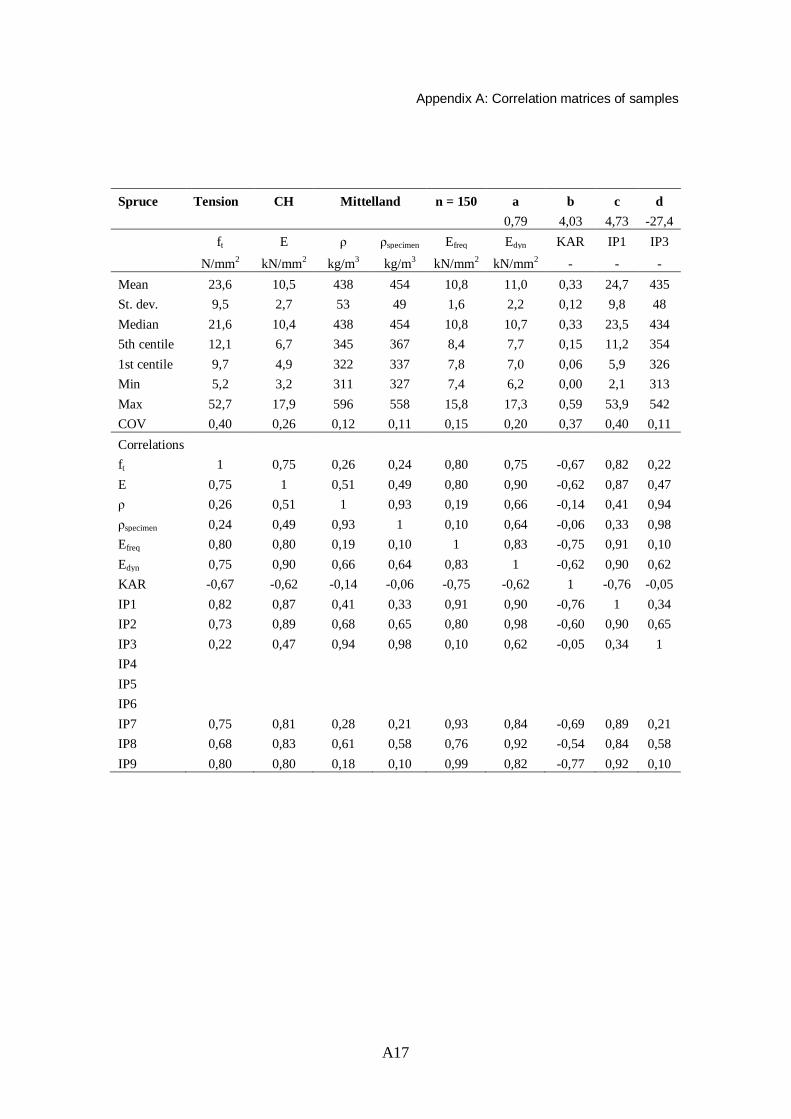
Appendix A: Correlation matrices of samples
A17
Spruce Tension CH Mittelland n = 150 a b c d
0,79 4,03 4,73 -27,4
ft E specimen Efreq Edyn KAR IP1 IP3
N/mm2 kN/mm2 kg/m3 kg/m3 kN/mm2 kN/mm2 - - - Mean 23,6 10,5 438 454 10,8 11,0 0,33 24,7 435 St. dev. 9,5 2,7 53 49 1,6 2,2 0,12 9,8 48 Median 21,6 10,4 438 454 10,8 10,7 0,33 23,5 434 5th centile 12,1 6,7 345 367 8,4 7,7 0,15 11,2 354 1st centile 9,7 4,9 322 337 7,8 7,0 0,06 5,9 326 Min 5,2 3,2 311 327 7,4 6,2 0,00 2,1 313 Max 52,7 17,9 596 558 15,8 17,3 0,59 53,9 542 COV 0,40 0,26 0,12 0,11 0,15 0,20 0,37 0,40 0,11 Correlations
ft 1 0,75 0,26 0,24 0,80 0,75 -0,67 0,82 0,22 E 0,75 1 0,51 0,49 0,80 0,90 -0,62 0,87 0,47 0,26 0,51 1 0,93 0,19 0,66 -0,14 0,41 0,94
specimen 0,24 0,49 0,93 1 0,10 0,64 -0,06 0,33 0,98 Efreq 0,80 0,80 0,19 0,10 1 0,83 -0,75 0,91 0,10 Edyn 0,75 0,90 0,66 0,64 0,83 1 -0,62 0,90 0,62 KAR -0,67 -0,62 -0,14 -0,06 -0,75 -0,62 1 -0,76 -0,05 IP1 0,82 0,87 0,41 0,33 0,91 0,90 -0,76 1 0,34 IP2 0,73 0,89 0,68 0,65 0,80 0,98 -0,60 0,90 0,65 IP3 0,22 0,47 0,94 0,98 0,10 0,62 -0,05 0,34 1 IP4
IP5 IP6 IP7 0,75 0,81 0,28 0,21 0,93 0,84 -0,69 0,89 0,21
IP8 0,68 0,83 0,61 0,58 0,76 0,92 -0,54 0,84 0,58 IP9 0,80 0,80 0,18 0,10 0,99 0,82 -0,77 0,92 0,10

Appendix A: Correlation matrices of samples
A18
Spruce Tension CH Voralpen/Alpen n = 149 a b c d
1,16 -2,11 5,93 -39,1
ft E specimen Efreq Edyn KAR IP1 IP3
N/mm2 kN/mm2 kg/m3 kg/m3 kN/mm2 kN/mm2 - - - Mean 27,3 10,5 429 443 11,2 11,0 0,29 25,4 419 St. dev. 11,3 2,1 41 55 1,4 2,0 0,10 8,3 38 Median 25,5 10,2 431 441 11,1 10,8 0,30 24,6 419 5th centile 13,1 8,0 367 379 9,3 8,4 0,13 13,0 357 1st centile 9,0 6,4 348 364 8,2 7,7 0,05 10,5 339 Min 5,9 4,4 326 349 7,5 6,8 0,00 8,6 326 Max 68,2 17,6 520 937 15,0 20,7 0,65 53,4 507 COV 0,41 0,20 0,09 0,12 0,12 0,19 0,33 0,33 0,09 Correlations
ft 1 0,80 0,51 0,38 0,73 0,76 -0,52 0,85 0,54 E 0,80 1 0,55 0,34 0,75 0,76 -0,44 0,82 0,57 0,51 0,55 1 0,70 0,31 0,69 -0,29 0,56 0,95
specimen 0,38 0,34 0,70 1 0,12 0,72 -0,18 0,35 0,70 Efreq 0,73 0,75 0,31 0,12 1 0,77 -0,45 0,83 0,28 Edyn 0,76 0,76 0,69 0,72 0,77 1 -0,43 0,81 0,67 KAR -0,52 -0,44 -0,29 -0,18 -0,45 -0,43 1 -0,51 -0,25 IP1 0,85 0,82 0,56 0,35 0,83 0,81 -0,51 1 0,58 IP2 0,82 0,86 0,74 0,52 0,79 0,91 -0,43 0,91 0,76 IP3 0,54 0,57 0,95 0,70 0,28 0,67 -0,25 0,58 1 IP4
IP5 IP6 IP7 0,72 0,78 0,33 0,16 0,91 0,74 -0,42 0,83 0,33
IP8 0,76 0,78 0,65 0,42 0,73 0,80 -0,33 0,84 0,68 IP9 0,74 0,76 0,30 0,12 0,95 0,74 -0,45 0,83 0,28

Appendix A: Correlation matrices of samples
A19
A2: Poland
Spruce Tension PL Swietjano n = 111 a b c d
0,98 1,16 4,97 -27,5
ft E speci-
men Efreq Edyn KAR IP1 IP3 N/mm2 kN/mm2 kg/m3 kg/m3 kN/mm2 kN/mm2 - - - Mean 31,4 12,4 472 475 11,8 12,6 0,27 30,8 452 St. dev. 11,5 2,7 51 46 1,5 2,3 0,11 9,1 47 Median 30,9 12,4 469 474 11,9 12,4 0,26 30,0 452 5th centile 14,6 8,6 390 405 9,3 9,1 0,11 15,5 375 1st centile 8,9 7,2 369 371 8,3 8,3 0,01 12,3 340 Min 5,9 6,0 345 358 7,6 7,6 0,00 8,7 336 Max 64,8 20,1 591 577 15,2 18,1 0,58 49,4 562 COV 0,37 0,22 0,11 0,10 0,13 0,18 0,42 0,29 0,11 Correlations
ft 1 0,80 0,45 0,38 0,66 0,69 -0,40 0,77 0,41 E 0,80 1 0,67 0,61 0,85 0,94 -0,37 0,91 0,62 0,45 0,67 1 0,97 0,39 0,79 -0,07 0,57 0,97 specimen 0,38 0,61 0,97 1 0,28 0,72 -0,04 0,49 0,98
Efreq 0,66 0,85 0,39 0,28 1 0,86 -0,39 0,90 0,29 Edyn 0,69 0,94 0,79 0,72 0,86 1 -0,31 0,91 0,72 KAR -0,40 -0,37 -0,07 -0,04 -0,39 -0,31 1 -0,46 -0,09 IP1 0,77 0,91 0,57 0,49 0,90 0,91 -0,46 1 0,51 IP2 0,71 0,94 0,80 0,73 0,84 0,99 -0,35 0,92 0,75 IP3 0,41 0,62 0,97 0,98 0,29 0,72 -0,09 0,51 1 IP4 0,68 0,86 0,67 0,63 0,81 0,90 -0,40 0,88 0,64 IP5 0,64 0,85 0,69 0,65 0,80 0,91 -0,30 0,84 0,64 IP6 0,37 0,51 0,72 0,76 0,26 0,59 -0,05 0,41 0,74 IP7 0,27 0,48 0,38 0,34 0,50 0,54 -0,26 0,45 0,33 IP8
IP9 0,66 0,85 0,37 0,27 0,99 0,85 -0,41 0,91 0,28

Appendix A: Correlation matrices of samples
A20
Spruce Tension PL Murow n = 111 a b c d
0,97 0,68 5,28 -34,2
ft E specimen Efreq Edyn KAR IP1 IP3
N/mm2 kN/mm2 kg/m3 kg/m3 kN/mm2 kN/mm2 - - - Mean 25,1 10,7 432 440 11,2 11,1 0,32 25,2 418 St. dev. 9,1 2,3 45 41 1,4 2,0 0,11 8,1 44 Median 23,6 10,4 431 435 11,3 10,9 0,32 25,0 414 5th centile 13,6 7,8 367 382 9,0 8,2 0,16 13,5 354 1st centile 11,4 6,6 339 350 8,3 7,3 0,10 7,2 323 Min 9,0 4,2 335 345 7,9 6,8 0,09 3,2 320 Max 57,4 17,8 591 583 14,2 17,2 0,69 52,5 567 COV 0,36 0,22 0,10 0,09 0,12 0,18 0,33 0,32 0,10 Correlations
ft 1 0,83 0,52 0,48 0,79 0,82 -0,53 0,86 0,52 E 0,83 1 0,71 0,69 0,79 0,93 -0,49 0,90 0,71 0,52 0,71 1 0,97 0,39 0,79 -0,39 0,60 0,98
specimen 0,48 0,69 0,97 1 0,31 0,75 -0,29 0,55 0,99 Efreq 0,79 0,79 0,39 0,31 1 0,86 -0,44 0,89 0,36 Edyn 0,82 0,93 0,79 0,75 0,86 1 -0,48 0,92 0,78 KAR -0,53 -0,49 -0,39 -0,29 -0,44 -0,48 1 -0,58 -0,37 IP1 0,86 0,90 0,60 0,55 0,89 0,92 -0,58 1 0,59 IP2 0,82 0,93 0,80 0,76 0,84 0,99 -0,48 0,91 0,80 IP3 0,52 0,71 0,98 0,99 0,36 0,78 -0,37 0,59 1 IP4 0,80 0,84 0,68 0,64 0,80 0,90 -0,48 0,84 0,68 IP5 0,78 0,84 0,70 0,67 0,79 0,91 -0,43 0,82 0,70 IP6 0,40 0,50 0,73 0,75 0,25 0,57 -0,20 0,37 0,74 IP7 0,38 0,36 0,13 0,10 0,57 0,43 -0,16 0,43 0,13 IP8
IP9 0,80 0,80 0,39 0,32 0,99 0,85 -0,45 0,89 0,36
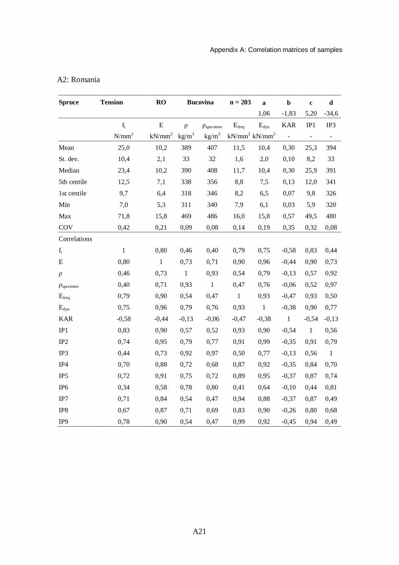
Appendix A: Correlation matrices of samples
A21
A2: Romania Spruce Tension RO Bucovina n = 203 a b c d
1,06 -1,83 5,20 -34,6
ft E specimen Efreq Edyn KAR IP1 IP3
N/mm2 kN/mm2 kg/m3 kg/m3 kN/mm2 kN/mm2 - - -
Mean 25,0 10,2 389 407 11,5 10,4 0,30 25,3 394
St. dev. 10,4 2,1 33 32 1,6 2,0 0,10 8,2 33
Median 23,4 10,2 390 408 11,7 10,4 0,30 25,9 391
5th centile 12,5 7,1 338 356 8,8 7,5 0,13 12,0 341
1st centile 9,7 6,4 318 346 8,2 6,5 0,07 9,8 326
Min 7,0 5,3 311 340 7,9 6,1 0,03 5,9 320
Max 71,8 15,8 469 486 16,0 15,8 0,57 49,5 480
COV 0,42 0,21 0,09 0,08 0,14 0,19 0,35 0,32 0,08
Correlations
ft 1 0,80 0,46 0,40 0,79 0,75 -0,58 0,83 0,44
E 0,80 1 0,73 0,71 0,90 0,96 -0,44 0,90 0,73
0,46 0,73 1 0,93 0,54 0,79 -0,13 0,57 0,92
specimen 0,40 0,71 0,93 1 0,47 0,76 -0,06 0,52 0,97
Efreq 0,79 0,90 0,54 0,47 1 0,93 -0,47 0,93 0,50
Edyn 0,75 0,96 0,79 0,76 0,93 1 -0,38 0,90 0,77
KAR -0,58 -0,44 -0,13 -0,06 -0,47 -0,38 1 -0,54 -0,13
IP1 0,83 0,90 0,57 0,52 0,93 0,90 -0,54 1 0,56
IP2 0,74 0,95 0,79 0,77 0,91 0,99 -0,35 0,91 0,79
IP3 0,44 0,73 0,92 0,97 0,50 0,77 -0,13 0,56 1
IP4 0,70 0,88 0,72 0,68 0,87 0,92 -0,35 0,84 0,70
IP5 0,72 0,91 0,75 0,72 0,89 0,95 -0,37 0,87 0,74
IP6 0,34 0,58 0,78 0,80 0,41 0,64 -0,10 0,44 0,81
IP7 0,71 0,84 0,54 0,47 0,94 0,88 -0,37 0,87 0,49
IP8 0,67 0,87 0,71 0,69 0,83 0,90 -0,26 0,80 0,68
IP9 0,78 0,90 0,54 0,47 0,99 0,92 -0,45 0,94 0,49

Appendix A: Correlation matrices of samples
A22
Spruce Tension RO Transylvania n = 116 a b c d
1,25 -5,06 5,82 -41,9
ft E specimen Efreq Edyn KAR IP1 IP3
N/mm2 kN/mm2 kg/m3 kg/m3 kN/mm2 kN/mm2 - - - Mean 26,7 9,8 391 404 11,8 10,5 0,32 25,3 387 St. dev. 11,6 2,1 32 30 1,6 1,8 0,11 8,0 31 Median 24,2 9,6 395 409 11,8 10,3 0,32 25,2 389 5th centile 12,4 6,5 330 349 9,2 7,5 0,15 13,0 327 1st centile 10,0 6,2 323 335 8,1 7,1 0,09 6,7 323 Min 9,7 6,1 322 332 7,6 7,1 0,05 6,7 318 Max 72,8 15,6 476 478 16,0 16,1 0,68 47,1 465 COV 0,44 0,21 0,08 0,08 0,13 0,18 0,34 0,32 0,08 Correlations
ft 1 0,82 0,54 0,44 0,79 0,81 -0,60 0,87 0,51 E 0,82 1 0,74 0,65 0,86 0,96 -0,45 0,87 0,70 0,54 0,74 1 0,95 0,43 0,76 -0,17 0,49 0,96
specimen 0,44 0,65 0,95 1 0,29 0,66 -0,04 0,36 0,99 Efreq 0,79 0,86 0,43 0,29 1 0,90 -0,52 0,93 0,37 Edyn 0,81 0,96 0,76 0,66 0,90 1 -0,42 0,89 0,73 KAR -0,60 -0,45 -0,17 -0,04 -0,52 -0,42 1 -0,60 -0,12 IP1 0,87 0,87 0,49 0,36 0,93 0,89 -0,60 1 0,45 IP2 0,81 0,95 0,77 0,68 0,89 1,00 -0,41 0,89 0,74 IP3 0,51 0,70 0,96 0,99 0,37 0,73 -0,12 0,45 1 IP4 0,84 0,93 0,67 0,55 0,89 0,94 -0,53 0,89 0,62 IP5 0,77 0,94 0,74 0,65 0,86 0,96 -0,40 0,84 0,70 IP6 0,47 0,69 0,97 0,98 0,32 0,69 -0,09 0,40 0,97 IP7 0,71 0,82 0,43 0,30 0,97 0,88 -0,45 0,88 0,38 IP8 0,68 0,84 0,64 0,59 0,85 0,91 -0,34 0,82 0,65 IP9 0,77 0,83 0,39 0,25 0,99 0,88 -0,51 0,93 0,34

Appendix A: Correlation matrices of samples
A23
A2: Sweden Spruce Tension SE Lapland n = 113 a b c d
0,73 9,06 3,44 -10,2
ft E speci-
men Efreq Edyn KAR IP1 IP3
N/mm2 kN/mm2 kg/m3 kg/m
3 kN/mm2 kN/mm2 - - - Mean 29,1 10,0 414 444 11,4 11,3 0,20 27,6 427 St. dev. 9,7 2,0 42 44 1,7 2,4 0,09 9,1 44 Median 27,8 10,1 413 446 11,5 11,0 0,20 27,6 430 5th centile 14,4 7,0 342 375 9,0 7,8 0,08 13,7 358 1st centile 7,0 5,3 333 346 7,2 6,4 0,04 6,5 328 Min 6,0 4,8 325 343 5,9 5,5 0,04 4,7 324 Max 59,4 14,6 520 546 15,6 19,1 0,56 53,5 545 COV 0,33 0,20 0,10 0,10 0,15 0,22 0,47 0,33 0,10 Correlations
ft 1 0,78 0,41 0,41 0,61 0,60 -0,48 0,69 0,46 E 0,78 1 0,52 0,54 0,65 0,69 -0,40 0,74 0,57 0,41 0,52 1 0,97 0,47 0,78 -0,13 0,59 0,95
specimen 0,41 0,54 0,97 1 0,47 0,79 -0,10 0,59 0,98 Efreq 0,61 0,65 0,47 0,47 1 0,91 -0,40 0,90 0,49 Edyn 0,60 0,69 0,78 0,79 0,91 1 -0,32 0,90 0,80 KAR -0,48 -0,40 -0,13 -0,10 -0,40 -0,32 1 -0,46 -0,15 IP1 0,69 0,74 0,59 0,59 0,90 0,90 -0,46 1 0,64 IP2 0,61 0,72 0,76 0,77 0,87 0,97 -0,31 0,93 0,80 IP3 0,46 0,57 0,95 0,98 0,49 0,80 -0,15 0,64 1 IP4 0,64 0,73 0,72 0,72 0,88 0,95 -0,39 0,93 0,76 IP5 0,61 0,74 0,75 0,76 0,86 0,96 -0,33 0,91 0,79 IP6 0,41 0,58 0,90 0,93 0,43 0,73 -0,16 0,55 0,95 IP7 0,59 0,68 0,48 0,48 0,90 0,85 -0,30 0,88 0,51 IP8 0,56 0,60 0,66 0,66 0,69 0,79 -0,21 0,73 0,66 IP9 0,60 0,67 0,47 0,47 0,95 0,88 -0,36 0,93 0,50

Appendix A: Correlation matrices of samples
A24
Spruce Tension SE Västergötland n = 105 a b c d
0,96 0,5 5,89 -41,5
ft E specimen Efreq Edyn KAR IP1 IP3
N/mm2 kN/mm2 kg/m3 kg/m3 kN/mm2 kN/mm2 - - -
Mean 25,9 10,4 418 447 11,5 11,5 0,28 26,4 431
St. dev. 11,4 2,7 54 57 1,6 2,7 0,11 10,6 60
Median 25,8 10,7 417 447 11,7 11,5 0,28 27,7 431
5th centile 9,9 6,6 337 363 8,9 7,6 0,13 11,5 339
1st centile 8,8 6,1 332 352 8,4 7,3 0,00 7,6 333
Min 7,0 4,5 328 349 8,3 7,1 0,00 3,1 332
Max 63,1 17,7 556 600 15,6 19,3 0,57 58,2 573
COV 0,44 0,26 0,13 0,13 0,14 0,23 0,40 0,40 0,14
Correlations
ft 1 0,86 0,68 0,69 0,82 0,86 -0,66 0,90 0,72
E 0,86 1 0,81 0,82 0,81 0,93 -0,59 0,89 0,84
0,68 0,81 1 0,98 0,56 0,87 -0,46 0,76 0,98
specimen 0,69 0,82 0,98 1 0,55 0,87 -0,46 0,76 0,99
Efreq 0,82 0,81 0,56 0,55 1 0,88 -0,54 0,92 0,58
Edyn 0,86 0,93 0,87 0,87 0,88 1 -0,57 0,96 0,89
KAR -0,66 -0,59 -0,46 -0,46 -0,54 -0,57 1 -0,63 -0,50
IP1 0,90 0,89 0,76 0,76 0,92 0,96 -0,63 1 0,78
IP2 0,86 0,92 0,88 0,87 0,88 1,00 -0,57 0,96 0,89
IP3 0,72 0,84 0,98 0,99 0,58 0,89 -0,50 0,78 1
IP4 0,86 0,91 0,85 0,84 0,86 0,98 -0,58 0,95 0,86
IP5 0,85 0,92 0,87 0,87 0,87 0,99 -0,56 0,95 0,88
IP6 0,69 0,82 0,97 0,99 0,54 0,87 -0,48 0,76 0,99
IP7 0,79 0,81 0,64 0,62 0,95 0,90 -0,53 0,92 0,65
IP8 0,77 0,86 0,83 0,84 0,78 0,92 -0,53 0,87 0,84
IP9 0,81 0,78 0,54 0,52 0,99 0,86 -0,56 0,90 0,54

Appendix A: Correlation matrices of samples
A25
A2: Slovenia Spruce Tension SI Upper Carniola n = 104 a b c d
1,19 -3,68 6,17 -43,9
ft E specimen Efreq Edyn KAR IP1 IP3
N/mm2 kN/mm2 kg/m3 kg/m3 kN/mm2 kN/mm2 - - - Mean 34,0 12,3 442 451 12,6 12,7 0,25 31,6 429 St. dev. 15,0 2,7 41 38 2,0 2,5 0,11 11,0 38 Median 31,8 12,2 441 452 12,7 12,5 0,25 31,1 426 5th centile 14,0 8,2 386 393 8,7 8,8 0,08 12,2 373 1st centile 10,0 6,9 361 384 7,7 7,7 0,05 6,4 365 Min 8,9 6,5 352 379 7,7 7,6 0,00 3,8 355 Max 89,6 18,7 535 534 16,4 19,1 0,6 56,5 505 COV 0,44 0,22 0,09 0,08 0,16 0,20 0,43 0,35 0,09 Correlations
ft 1 0,83 0,44 0,36 0,81 0,81 -0,62 0,87 0,44 E 0,83 1 0,63 0,57 0,92 0,98 -0,53 0,94 0,63 0,44 0,63 1 0,96 0,34 0,69 -0,26 0,48 0,97
specimen 0,36 0,57 0,96 1 0,24 0,63 -0,16 0,40 0,98 Efreq 0,81 0,92 0,34 0,24 1 0,91 -0,55 0,93 0,33 Edyn 0,81 0,98 0,69 0,63 0,91 1 -0,50 0,92 0,68 KAR -0,62 -0,53 -0,26 -0,16 -0,55 -0,50 1 -0,64 -0,26 IP1 0,87 0,94 0,48 0,40 0,93 0,92 -0,64 1 0,49 IP2 0,80 0,98 0,71 0,65 0,88 0,99 -0,48 0,92 0,71 IP3 0,44 0,63 0,97 0,98 0,33 0,68 -0,26 0,49 1 IP4 0,81 0,95 0,66 0,60 0,87 0,96 -0,53 0,91 0,66 IP5 0,77 0,95 0,69 0,64 0,86 0,97 -0,46 0,90 0,69 IP6 0,32 0,49 0,85 0,88 0,20 0,54 -0,13 0,36 0,89 IP7 0,71 0,87 0,41 0,31 0,93 0,87 -0,45 0,86 0,38 IP8 0,71 0,92 0,67 0,61 0,84 0,94 -0,39 0,85 0,66 IP9 0,81 0,92 0,34 0,25 0,99 0,90 -0,53 0,93 0,32

Appendix A: Correlation matrices of samples
A26
A2: Slovakia Spruce Tension SK Prešov n = 115 a b c d
1,20 3,57 5,95 -43,3
ft E specimen Efreq Edyn KAR IP1 IP3
N/mm2 kN/mm2 kg/m3 kg/m3 kN/mm2 kN/mm2 - - -
Mean 28,3 10,7 401 416 12,0 11,1 0,26 26,6 395
St. dev. 12,1 2,2 33 32 1,7 2,1 0,08 8,8 33
Median 25,8 10,6 395 412 12,2 11,1 0,26 26,1 390
5th centile 13,4 7,1 354 373 9,2 7,9 0,13 12,6 351
1st centile 8,4 6,0 348 361 7,7 6,4 0,08 5,7 341
Min 7,0 5,9 340 350 7,4 6,3 0,08 3,3 332
Max 70,3 18,2 507 538 15,6 18,6 0,51 52,3 521
COV 0,43 0,21 0,08 0,08 0,14 0,19 0,32 0,33 0,08
Correlations
ft 1 0,86 0,56 0,55 0,82 0,84 -0,62 0,88 0,61
E 0,86 1 0,75 0,74 0,91 0,99 -0,60 0,95 0,80
0,56 0,75 1 0,97 0,50 0,78 -0,41 0,64 0,98
specimen 0,55 0,74 0,97 1 0,45 0,77 -0,37 0,61 0,99
Efreq 0,82 0,91 0,50 0,45 1 0,92 -0,57 0,94 0,54
Edyn 0,84 0,99 0,78 0,77 0,92 1 -0,57 0,95 0,83
KAR -0,62 -0,60 -0,41 -0,37 -0,57 -0,57 1 -0,65 -0,43
IP1 0,88 0,95 0,64 0,61 0,94 0,95 -0,65 1 0,69
IP2 0,84 0,98 0,79 0,77 0,91 0,99 -0,57 0,95 0,83
IP3 0,61 0,80 0,98 0,99 0,54 0,83 -0,43 0,69 1
IP4 0,84 0,95 0,71 0,68 0,92 0,96 -0,64 0,94 0,75
IP5 0,79 0,95 0,76 0,73 0,88 0,96 -0,54 0,91 0,79
IP6 0,54 0,74 0,97 0,99 0,46 0,77 -0,37 0,61 0,98
IP7 0,78 0,88 0,49 0,46 0,97 0,89 -0,57 0,90 0,54
IP8 0,78 0,93 0,76 0,75 0,82 0,93 -0,53 0,87 0,80
IP9 0,83 0,91 0,49 0,45 0,99 0,91 -0,58 0,93 0,53

Appendix A: Correlation matrices of samples
A27
Spruce Tension SK Žilina n = 100 a b c d
1,06 -0,69 5,43 -37,6
ft E specimen Efreq Edyn KAR IP1 IP3
N/mm2 kN/mm2 kg/m3 kg/m3 kN/mm2 kN/mm2 - - -
Mean 25,9 10,7 416 426 11,7 11,0 0,29 24,7 401
St. dev. 9,3 2,0 38 36 1,3 1,9 0,09 7,5 36
Median 24,1 10,7 413 421 11,7 10,7 0,29 23,2 394
5th centile 13,6 7,5 354 366 9,6 8,0 0,16 13,1 342
1st centile 9,9 7,1 341 354 9,3 7,7 0,12 10,7 334
Min 6,8 6,8 334 345 9,0 7,7 0,10 10,3 325
Max 55,3 17,0 516 523 14,8 17,1 0,51 47 508
COV 0,36 0,19 0,09 0,09 0,11 0,17 0,29 0,30 0,09
Correlations
ft 1 0,81 0,49 0,44 0,76 0,74 -0,54 0,86 0,51
E 0,81 1 0,76 0,71 0,88 0,96 -0,29 0,90 0,76
0,49 0,76 1 0,96 0,49 0,82 -0,10 0,60 0,96
specimen 0,44 0,71 0,96 1 0,43 0,79 -0,03 0,57 0,99
Efreq 0,76 0,88 0,49 0,43 1 0,88 -0,24 0,88 0,49
Edyn 0,74 0,96 0,82 0,79 0,88 1 -0,18 0,88 0,83
KAR -0,54 -0,29 -0,10 -0,03 -0,24 -0,18 1 -0,42 -0,07
IP1 0,86 0,90 0,60 0,57 0,88 0,88 -0,42 1 0,64
IP2 0,75 0,95 0,80 0,78 0,88 0,99 -0,19 0,90 0,83
IP3 0,51 0,76 0,96 0,99 0,49 0,83 -0,07 0,64 1
IP4 0,67 0,85 0,74 0,77 0,78 0,91 -0,15 0,82 0,79
IP5 0,68 0,88 0,80 0,80 0,79 0,94 -0,12 0,82 0,83
IP6 0,42 0,64 0,78 0,85 0,43 0,72 0,07 0,54 0,85
IP7 0,62 0,81 0,49 0,45 0,92 0,83 -0,18 0,79 0,49
IP8 0,56 0,83 0,77 0,76 0,76 0,89 -0,10 0,73 0,78
IP9 0,77 0,88 0,48 0,43 0,99 0,87 -0,28 0,89 0,49
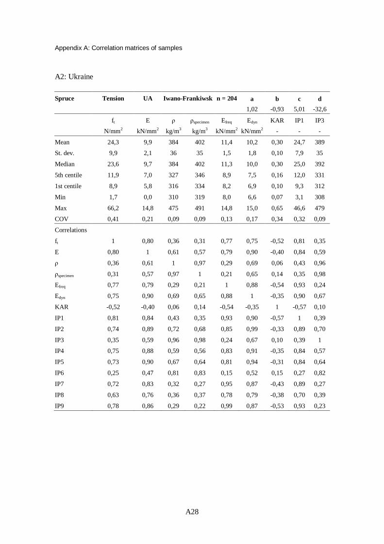
Appendix A: Correlation matrices of samples
A28
A2: Ukraine Spruce Tension UA Iwano-Frankiwsk n = 204 a b c d
1,02 -0,93 5,01 -32,6
ft E specimen Efreq Edyn KAR IP1 IP3
N/mm2 kN/mm2 kg/m3 kg/m3 kN/mm2 kN/mm2 - - -
Mean 24,3 9,9 384 402 11,4 10,2 0,30 24,7 389
St. dev. 9,9 2,1 36 35 1,5 1,8 0,10 7,9 35
Median 23,6 9,7 384 402 11,3 10,0 0,30 25,0 392
5th centile 11,9 7,0 327 346 8,9 7,5 0,16 12,0 331
1st centile 8,9 5,8 316 334 8,2 6,9 0,10 9,3 312
Min 1,7 0,0 310 319 8,0 6,6 0,07 3,1 308
Max 66,2 14,8 475 491 14,8 15,0 0,65 46,6 479
COV 0,41 0,21 0,09 0,09 0,13 0,17 0,34 0,32 0,09
Correlations
ft 1 0,80 0,36 0,31 0,77 0,75 -0,52 0,81 0,35
E 0,80 1 0,61 0,57 0,79 0,90 -0,40 0,84 0,59
0,36 0,61 1 0,97 0,29 0,69 0,06 0,43 0,96
specimen 0,31 0,57 0,97 1 0,21 0,65 0,14 0,35 0,98
Efreq 0,77 0,79 0,29 0,21 1 0,88 -0,54 0,93 0,24
Edyn 0,75 0,90 0,69 0,65 0,88 1 -0,35 0,90 0,67
KAR -0,52 -0,40 0,06 0,14 -0,54 -0,35 1 -0,57 0,10
IP1 0,81 0,84 0,43 0,35 0,93 0,90 -0,57 1 0,39
IP2 0,74 0,89 0,72 0,68 0,85 0,99 -0,33 0,89 0,70
IP3 0,35 0,59 0,96 0,98 0,24 0,67 0,10 0,39 1
IP4 0,75 0,88 0,59 0,56 0,83 0,91 -0,35 0,84 0,57
IP5 0,73 0,90 0,67 0,64 0,81 0,94 -0,31 0,84 0,64
IP6 0,25 0,47 0,81 0,83 0,15 0,52 0,15 0,27 0,82
IP7 0,72 0,83 0,32 0,27 0,95 0,87 -0,43 0,89 0,27
IP8 0,63 0,76 0,36 0,37 0,78 0,79 -0,38 0,70 0,39
IP9 0,78 0,86 0,29 0,22 0,99 0,87 -0,53 0,93 0,23

Appendix A: Correlation matrices of samples
A29
Spruce Tension UA Lemberg n = 125 a b c d
1,26 -4,38 6,04 -43,9
ft E specimen Efreq Edyn KAR IP1 IP3
N/mm2 kN/mm2 kg/m3 kg/m3 kN/mm2 kN/mm2 - - -
Mean 30,5 11,0 405 417 12,3 11,4 0,28 27,7 394
St. dev. 13,5 2,2 49 46 1,6 2,2 0,10 8,8 47
Median 29,4 10,9 402 420 12,4 11,4 0,27 28,2 393
5th centile 12,5 7,6 339 357 9,7 7,9 0,10 13,8 334
1st centile 10,3 6,8 306 319 9,1 7,1 0,08 10,0 296
Min 8,3 6,6 304 318 8,9 6,9 0,08 9,4 296
Max 74,6 18,0 545 551 16,5 18,2 0,55 53,2 536
COV 0,44 0,20 0,12 0,11 0,13 0,20 0,38 0,32 0,12
Correlations
ft 1 0,78 0,55 0,47 0,72 0,74 -0,62 0,82 0,54
E 0,78 1 0,79 0,76 0,83 0,99 -0,36 0,92 0,80
0,55 0,79 1 0,97 0,39 0,81 -0,22 0,61 0,97
specimen 0,47 0,76 0,97 1 0,32 0,78 -0,11 0,55 0,99
Efreq 0,72 0,83 0,39 0,32 1 0,84 -0,40 0,90 0,39
Edyn 0,74 0,99 0,81 0,78 0,84 1 -0,32 0,91 0,82
KAR -0,62 -0,36 -0,22 -0,11 -0,40 -0,32 1 -0,46 -0,17
IP1 0,82 0,92 0,61 0,55 0,90 0,91 -0,46 1 0,62
IP2 0,74 0,98 0,83 0,80 0,80 0,99 -0,32 0,91 0,84
IP3 0,54 0,80 0,97 0,99 0,39 0,82 -0,17 0,62 1
IP4 0,80 0,97 0,75 0,70 0,85 0,97 -0,43 0,95 0,76
IP5 0,74 0,98 0,81 0,79 0,81 0,99 -0,32 0,91 0,83
IP6 0,47 0,74 0,96 0,99 0,30 0,76 -0,11 0,54 0,99
IP7 0,67 0,85 0,47 0,43 0,92 0,85 -0,31 0,88 0,49
IP8 0,71 0,93 0,72 0,70 0,81 0,94 -0,28 0,88 0,75
IP9 0,69 0,81 0,37 0,30 0,94 0,79 -0,38 0,87 0,36

Appendix A: Correlation matrices of samples
A30
A3: Poland
Pine Bending PL Murow n = 110 a b c d
0,94 -1,24 6,23 -22,60
fm Eglobal specimen Efreq Edyn KAR IP1 IP3
N/mm2 kN/mm2 kg/m3 kg/m3 kN/mm2 kN/mm2 - - - Mean 42,0 12,4 539 558 10,4 12,9 0,24 46,1 532 St. dev. 17,1 2,7 54 61 1,7 2,9 0,17 14,1 66 Median 39,9 12,6 536 553 10,4 13,2 0,21 46,8 531 5th centile 16,5 7,8 448 461 7,5 8,3 0,02 23,3 429 1st centile 13,1 6,5 433 451 7,1 7,9 0,00 8,9 408 Min 9,2 5,0 425 439 6,9 7,3 0,00 8,1 396 Max 89,9 17,8 638 687 14,3 19,8 0,8 76,8 678 COV 0,41 0,22 0,10 0,11 0,16 0,22 0,72 0,31 0,12 Correlations
fm 1 0,76 0,53 0,52 0,62 0,70 -0,65 0,78 0,56 Eglobal 0,76 1 0,71 0,70 0,79 0,90 -0,61 0,84 0,74 0,53 0,71 1 0,96 0,37 0,72 -0,47 0,65 0,95
specimen 0,52 0,70 0,96 1 0,36 0,73 -0,47 0,65 0,98 Efreq 0,62 0,79 0,37 0,36 1 0,90 -0,59 0,80 0,41 Edyn 0,70 0,90 0,72 0,73 0,90 1 -0,65 0,88 0,75 KAR -0,65 -0,61 -0,47 -0,47 -0,59 -0,65 1 -0,75 -0,52 IP1 0,78 0,84 0,65 0,65 0,80 0,88 -0,75 1 0,69 IP2 0,69 0,91 0,70 0,69 0,87 0,96 -0,63 0,90 0,74 IP3 0,56 0,74 0,95 0,98 0,41 0,75 -0,52 0,69 1 IP4 0,65 0,73 0,57 0,58 0,74 0,81 -0,62 0,79 0,60 IP5 0,59 0,78 0,59 0,58 0,85 0,89 -0,56 0,82 0,61 IP6 0,41 0,59 0,78 0,80 0,38 0,65 -0,36 0,54 0,78 IP7 0,57 0,81 0,59 0,56 0,86 0,90 -0,56 0,81 0,60 IP8 0,58 0,82 0,67 0,66 0,82 0,91 -0,58 0,82 0,69 IP9 0,57 0,75 0,32 0,29 0,97 0,85 -0,56 0,78 0,35

Appendix A: Correlation matrices of samples
A31
Pine Bending PL Swietjano n = 111 a b c d
0,98 1,61 8,40 -45,34
fm Eglobal specimen Efreq Edyn KAR IP1 IP3
N/mm2 kN/mm2 kg/m3 kg/m3 kN/mm2 kN/mm2 - - - Mean 36,5 10,9 493 515 9,7 11,2 0,28 35,6 488 St. dev. 16,2 2,5 43 46 1,4 2,2 0,13 13,8 51 Median 34,5 10,5 488 512 9,7 10,9 0,26 35,5 486 5th centile 14,7 7,3 432 448 7,5 8,2 0,10 14,6 410 1st centile 12,9 6,9 414 419 7,3 7,4 0,09 5,9 397 Min 11,7 6,3 381 416 7,0 6,9 0,08 4,8 373 Max 77,2 18,1 620 641 13,4 17,5 0,6 66,2 626 COV 0,44 0,23 0,09 0,09 0,14 0,20 0,47 0,39 0,11 Correlations
fm 1 0,80 0,43 0,45 0,72 0,74 -0,54 0,83 0,53 Eglobal 0,80 1 0,69 0,71 0,82 0,94 -0,53 0,89 0,76
0,43 0,69 1 0,94 0,35 0,71 -0,23 0,54 0,90
specimen 0,45 0,71 0,94 1 0,35 0,72 -0,31 0,56 0,98 Efreq 0,72 0,82 0,35 0,35 1 0,89 -0,52 0,83 0,43 Edyn 0,74 0,94 0,71 0,72 0,89 1 -0,50 0,87 0,77 KAR -0,54 -0,53 -0,23 -0,31 -0,52 -0,50 1 -0,62 -0,38 IP1 0,83 0,89 0,54 0,56 0,83 0,87 -0,62 1 0,64 IP2 0,75 0,93 0,70 0,71 0,88 0,99 -0,48 0,88 0,77 IP3 0,53 0,76 0,90 0,98 0,43 0,77 -0,38 0,64 1 IP4 0,79 0,84 0,49 0,49 0,84 0,85 -0,52 0,85 0,56 IP5 0,73 0,88 0,61 0,63 0,87 0,94 -0,44 0,84 0,69 IP6 0,45 0,61 0,74 0,80 0,36 0,64 -0,20 0,53 0,80 IP7 0,70 0,87 0,63 0,61 0,86 0,93 -0,46 0,84 0,66 IP8 0,69 0,86 0,68 0,67 0,82 0,92 -0,47 0,83 0,71 IP9 0,71 0,81 0,36 0,33 0,98 0,87 -0,48 0,82 0,41

Appendix A: Correlation matrices of samples
A32
A3: Sweden
Pine Bending SE Lapland n = 34 a b c d
1,26 -11,3 8,62 -45,5
fm Eglobal specimen Efreq Edyn KAR IP1 IP3
N/mm2 kN/mm2 kg/m3 kg/m3 kN/mm2 kN/mm2 - - - Mean 37,8 9,1 458 484 9,7 10,4 0,24 38,9 460 St. dev. 15,7 2,1 44 43 1,5 2,4 0,08 11,5 43 Median 31,3 8,6 450 474 9,7 10,2 0,25 36,7 451 5th centile 19,6 6,7 407 440 7,6 7,6 0,09 23,3 414 1st centile 18,8 6,5 398 422 7,0 7,3 0,08 20,5 399 Min 18,6 6,4 397 414 6,7 7,2 0,08 20,5 393 Max 76,8 15,4 594 617 13,2 18,1 0,39 69,4 599 COV 0,41 0,23 0,10 0,09 0,15 0,23 0,33 0,30 0,09 Correlations
fm 1 0,92 0,59 0,66 0,82 0,87 -0,67 0,93 0,70 Eglobal 0,92 1 0,74 0,77 0,90 0,97 -0,58 0,93 0,80
0,59 0,74 1 0,96 0,50 0,78 -0,35 0,63 0,97
specimen 0,66 0,77 0,96 1 0,50 0,80 -0,36 0,65 0,98 Efreq 0,82 0,90 0,50 0,50 1 0,92 -0,60 0,91 0,57 Edyn 0,87 0,97 0,78 0,80 0,92 1 -0,60 0,93 0,84 KAR -0,67 -0,58 -0,35 -0,36 -0,60 -0,60 1 -0,72 -0,44 IP1 0,93 0,93 0,63 0,65 0,91 0,93 -0,72 1 0,72 IP2 0,86 0,97 0,77 0,78 0,93 1,00 -0,60 0,93 0,83 IP3 0,70 0,80 0,97 0,98 0,57 0,84 -0,44 0,72 1 IP4 0,89 0,91 0,62 0,66 0,83 0,88 -0,64 0,90 0,70 IP5 0,88 0,97 0,73 0,75 0,94 0,98 -0,58 0,94 0,79 IP6 0,61 0,71 0,92 0,95 0,45 0,74 -0,36 0,59 0,95 IP7 0,78 0,86 0,60 0,61 0,92 0,91 -0,55 0,88 0,66 IP8 0,74 0,83 0,63 0,64 0,87 0,89 -0,51 0,84 0,69 IP9 0,82 0,89 0,48 0,49 1,00 0,91 -0,58 0,91 0,55

Appendix A: Correlation matrices of samples
A33
Pine Bending SE Västerbotten n = 35 a b c d
1,22 -7,09 7,18 -21,4
fm Eglobal speci-
men Efreq Edyn KAR IP1 IP3
N/mm2 kN/mm2 kg/m3 kg/m3 kN/mm2 kN/mm2 - - - Mean 56,4 11,8 500 522 10,8 12,6 0,14 52,0 511 St. dev. 12,8 2,4 48 49 1,3 2,3 0,08 9,1 50 Median 57,4 11,7 499 516 11,0 12,6 0,13 52,3 504 5th centile 32,2 8,1 440 450 8,7 8,7 0,03 34,7 443 1st centile 29,4 7,7 396 417 8,0 8,1 0,03 31,1 400 Min 29,3 7,5 376 404 7,8 7,9 0,03 30,9 385 Max 80,9 16,8 585 603 13,0 17,2 0,31 69,5 591 COV 0,23 0,20 0,10 0,09 0,12 0,18 0,58 0,18 0,10 Correlations
fm 1 0,77 0,63 0,57 0,73 0,77 -0,41 0,87 0,61 Eglobal 0,77 1 0,79 0,82 0,81 0,96 -0,11 0,86 0,84
0,63 0,79 1 0,95 0,47 0,79 -0,25 0,77 0,96 specimen 0,57 0,82 0,95 1 0,45 0,81 -0,08 0,73 0,99
Efreq 0,73 0,81 0,47 0,45 1 0,89 -0,14 0,81 0,49 Edyn 0,77 0,96 0,79 0,81 0,89 1 -0,11 0,90 0,83 KAR -0,41 -0,11 -0,25 -0,08 -0,14 -0,11 1 -0,35 -0,10 IP1 0,87 0,86 0,77 0,73 0,81 0,90 -0,35 1 0,78 IP2 0,78 0,96 0,78 0,79 0,90 1,00 -0,11 0,91 0,82 IP3 0,61 0,84 0,96 0,99 0,49 0,83 -0,10 0,78 1 IP4 0,84 0,83 0,68 0,63 0,82 0,86 -0,38 0,94 0,68 IP5 0,78 0,96 0,78 0,79 0,89 0,99 -0,12 0,91 0,81 IP6 0,56 0,82 0,95 0,99 0,45 0,80 -0,06 0,71 0,99 IP7 0,68 0,92 0,72 0,74 0,87 0,96 -0,01 0,84 0,76 IP8 0,66 0,92 0,77 0,79 0,82 0,95 0,01 0,82 0,81 IP9 0,71 0,76 0,45 0,41 0,95 0,83 -0,16 0,76 0,45

Appendix A: Correlation matrices of samples
A34
Pine Bending SE Västergötland n = 140 a b c d
1,11 -3,38 7,15 -30,0
fm Eglobal specimen Efreq Edyn KAR IP1 IP3
N/mm2 kN/mm2 kg/m3 kg/m3 kN/mm2 kN/mm2 - - - Mean 43,5 10,9 482 509 10,3 11,6 0,22 42,2 489 St. dev. 13,9 1,8 42 39 1,1 1,8 0,10 9,9 40 Median 41,8 10,7 479 506 10,4 11,4 0,22 41,9 488 5th centile 24,3 8,3 423 452 8,5 8,9 0,06 26,2 435 1st centile 16,3 7,7 402 438 7,7 8,2 0,03 20,7 413 Min 15,3 6,8 395 424 7,6 7,5 0,03 16,0 403 Max 85,9 16,4 618 611 13,2 16,8 0,47 68,6 586 COV 0,32 0,16 0,09 0,08 0,11 0,15 0,46 0,24 0,08 Correlations
fm 1 0,76 0,58 0,55 0,59 0,71 -0,64 0,79 0,60 Eglobal 0,76 1 0,67 0,71 0,74 0,91 -0,55 0,80 0,74 0,58 0,67 1 0,90 0,36 0,72 -0,36 0,64 0,91
specimen 0,55 0,71 0,90 1 0,28 0,70 -0,33 0,56 0,98 Efreq 0,59 0,74 0,36 0,28 1 0,88 -0,52 0,76 0,36 Edyn 0,71 0,91 0,72 0,70 0,88 1 -0,55 0,84 0,75 KAR -0,64 -0,55 -0,36 -0,33 -0,52 -0,55 1 -0,69 -0,37 IP1 0,79 0,80 0,64 0,56 0,76 0,84 -0,69 1 0,64 IP2 0,71 0,89 0,71 0,68 0,88 0,99 -0,54 0,85 0,74 IP3 0,60 0,74 0,91 0,98 0,36 0,75 -0,37 0,64 1 IP4 0,72 0,80 0,62 0,61 0,65 0,79 -0,67 0,79 0,66 IP5 0,67 0,88 0,71 0,70 0,84 0,97 -0,53 0,79 0,74 IP6 0,49 0,67 0,87 0,96 0,24 0,66 -0,33 0,48 0,94 IP7 0,61 0,69 0,54 0,48 0,78 0,81 -0,37 0,74 0,55 IP8 0,61 0,70 0,59 0,55 0,73 0,81 -0,37 0,72 0,61 IP9 0,53 0,65 0,33 0,21 0,95 0,81 -0,46 0,73 0,29

Appendix A: Correlation matrices of samples
A35
A4: Finland
Pine Tension FI East n = 172 a b c d
1,16 -3,34 7,13 -45,5
ft E specimen Efreq Edyn KAR IP1 IP3
N/mm2 kN/mm2 kg/m3 kg/m3 kN/mm2 kN/mm2 - - - Mean 32,1 11,4 491 505 10,9 12,3 0,25 30,5 483 St. dev. 12,2 2,2 48 39 1,3 2,2 0,10 9,1 40 Median 30,9 11,4 484 501 11,0 12,2 0,24 30,9 480 5th centile 16,0 8,0 433 452 8,8 9,0 0,10 17,5 427 1st centile 12,3 7,3 397 414 7,9 7,6 0,04 11,6 392 Min 10,2 6,0 372 398 7,2 7,1 0,03 10,5 376 Max 73,2 17,2 623 618 13,8 17,7 0,48 51,1 598 COV 0,38 0,20 0,10 0,08 0,12 0,18 0,40 0,30 0,08 Correlations
ft 1 0,82 0,64 0,73 0,76 0,84 -0,77 0,86 0,75 E 0,82 1 0,65 0,80 0,88 0,94 -0,65 0,91 0,80 0,64 0,65 1 0,87 0,49 0,71 -0,53 0,67 0,87 specimen 0,73 0,80 0,87 1 0,60 0,84 -0,59 0,80 0,98
Efreq 0,76 0,88 0,49 0,60 1 0,93 -0,61 0,88 0,62 Edyn 0,84 0,94 0,71 0,84 0,93 1 -0,67 0,95 0,85 KAR -0,77 -0,65 -0,53 -0,59 -0,61 -0,67 1 -0,76 -0,61 IP1 0,86 0,91 0,67 0,80 0,88 0,95 -0,76 1 0,83 IP2 0,84 0,95 0,70 0,84 0,92 0,99 -0,68 0,95 0,86 IP3 0,75 0,80 0,87 0,98 0,62 0,85 -0,61 0,83 1 IP4 0,86 0,91 0,66 0,77 0,88 0,94 -0,72 0,93 0,78 IP5 0,83 0,93 0,69 0,82 0,89 0,97 -0,67 0,93 0,83 IP6 0,71 0,78 0,87 0,98 0,57 0,82 -0,58 0,77 0,97 IP7 0,62 0,69 0,37 0,46 0,81 0,74 -0,45 0,68 0,49 IP8
IP9 0,76 0,89 0,47 0,59 0,99 0,92 -0,63 0,88 0,62

Appendix A: Correlation matrices of samples
A36
Pine Tension FI West n = 85 a b c d
1,18 -3,98 8,60 -60,76
ft E specimen Efreq Edyn KAR IP1 IP3
N/mm2 kN/mm2 kg/m3 kg/m3 kN/mm2 kN/mm2 - - - Mean 31,0 11,3 493 508 10,7 12,1 0,27 29,6 486 St. dev. 12,9 2,3 59 46 1,2 2,3 0,11 9,7 47 Median 27,2 11,0 476 500 10,6 11,6 0,28 29,3 478 5th centile 17,8 7,9 419 444 8,8 9,2 0,09 15,9 421 1st centile 13,7 7,0 407 436 8,3 8,1 0,07 12,8 404 Min 11,3 6,8 400 432 8,1 7,7 0,06 11,9 401 Max 69,6 17,2 676 643 13,9 18,8 0,53 53,3 617 COV 0,41 0,21 0,12 0,09 0,11 0,19 0,41 0,33 0,10 Correlations
ft 1 0,85 0,72 0,76 0,80 0,87 -0,70 0,89 0,77 E 0,85 1 0,80 0,85 0,85 0,94 -0,63 0,93 0,86 0,72 0,80 1 0,92 0,64 0,83 -0,52 0,80 0,92
specimen 0,76 0,85 0,92 1 0,65 0,89 -0,52 0,83 0,99 Efreq 0,80 0,85 0,64 0,65 1 0,92 -0,55 0,89 0,65 Edyn 0,87 0,94 0,83 0,89 0,92 1 -0,60 0,95 0,88 KAR -0,70 -0,63 -0,52 -0,52 -0,55 -0,60 1 -0,69 -0,52 IP1 0,89 0,93 0,80 0,83 0,89 0,95 -0,69 1 0,84 IP2 0,87 0,96 0,83 0,88 0,92 0,99 -0,59 0,96 0,88 IP3 0,77 0,86 0,92 0,99 0,65 0,88 -0,52 0,84 1 IP4 0,86 0,92 0,80 0,83 0,87 0,94 -0,68 0,91 0,82 IP5 0,86 0,96 0,84 0,88 0,89 0,98 -0,61 0,94 0,88 IP6 0,77 0,85 0,91 0,99 0,64 0,88 -0,54 0,82 0,98 IP7 0,60 0,62 0,47 0,47 0,74 0,68 -0,44 0,65 0,46 IP8
IP9 0,78 0,89 0,62 0,64 0,98 0,90 -0,55 0,89 0,64

Appendix A: Correlation matrices of samples
A37
A4: France Pine Tension FR -600 m n = 130 a b c d
0,59 6,24 2,89 -6,74
ft E specimen Efreq Edyn KAR IP1 IP3
N/mm2 kN/mm2 kg/m3 kg/m3 kN/mm2 kN/mm2 - - - Mean 17,3 8,4 492 518 8,3 9,5 0,34 18,3 502 St. dev. 7,1 2,1 34 37 1,6 2,0 0,12 8,2 38 Median 15,2 8,3 490 517 8,1 9,3 0,33 16,9 505 5th centile 8,3 5,4 438 457 6,2 6,8 0,14 5,8 443 1st centile 7,2 4,2 422 450 5,7 6,4 0,12 4,2 435 Min 7,0 4,0 409 438 5,7 6,1 0,11 1,7 424 Max 44,4 14,6 585 617 19,5 21,0 0,67 38,3 606 COV 0,41 0,25 0,07 0,07 0,19 0,21 0,36 0,45 0,08 Correlations
ft 1 0,71 0,37 0,34 0,66 0,71 -0,40 0,73 0,43 E 0,71 1 0,41 0,46 0,65 0,74 -0,35 0,68 0,50 0,37 0,41 1 0,91 0,17 0,46 -0,18 0,48 0,88
specimen 0,34 0,46 0,91 1 0,13 0,45 -0,17 0,45 0,94 Efreq 0,66 0,65 0,17 0,13 1 0,94 -0,23 0,86 0,21 Edyn 0,71 0,74 0,46 0,45 0,94 1 -0,28 0,90 0,51 KAR -0,40 -0,35 -0,18 -0,17 -0,23 -0,28 1 -0,47 -0,22 IP1 0,73 0,68 0,48 0,45 0,86 0,90 -0,47 1 0,58 IP2 0,55 0,66 0,50 0,51 0,59 0,73 -0,41 0,91 0,65 IP3 0,43 0,50 0,88 0,94 0,21 0,51 -0,22 0,58 1 IP4 0,66 0,66 0,48 0,50 0,85 0,91 -0,43 0,86 0,61 IP5 0,53 0,60 0,52 0,53 0,53 0,68 -0,33 0,87 0,65 IP6 0,31 0,36 0,75 0,84 0,08 0,36 -0,13 0,38 0,83 IP7 0,53 0,54 0,19 0,14 0,92 0,82 -0,23 0,75 0,28 IP8
IP9 0,46 0,56 0,23 0,22 0,61 0,64 -0,39 0,85 0,36

Appendix A: Correlation matrices of samples
A38
Pine Tension FR +600 m n = 125 a b c d
0,69 5,94 3,25 -5,74
ft E specimen Efreq Edyn KAR IP1 IP3
N/mm2 kN/mm2 kg/m3 kg/m3 kN/mm2 kN/mm2 - - - Mean 23,8 9,8 532 568 9,1 11,4 0,30 25,7 554 St. dev. 8,2 2,1 46 50 1,4 2,1 0,12 8,0 49 Median 23,6 9,9 528 563 9,2 11,3 0,29 25,3 551 5th centile 11,0 5,9 469 500 6,5 8,0 0,12 13,2 490 1st centile 8,4 5,1 416 443 5,9 6,4 0,05 10,1 431 Min 5,9 2,3 402 431 5,5 6,1 0,04 7,8 415 Max 48,5 16,6 645 710 13,4 19,6 0,61 57 695 COV 0,34 0,22 0,09 0,09 0,16 0,18 0,38 0,31 0,09 Correlations
ft 1 0,77 0,24 0,24 0,56 0,60 -0,43 0,68 0,32 E 0,77 1 0,27 0,27 0,60 0,65 -0,34 0,68 0,35 0,24 0,27 1 0,96 0,04 0,46 -0,10 0,38 0,92
specimen 0,24 0,27 0,96 1 -0,01 0,44 -0,08 0,36 0,97 Efreq 0,56 0,60 0,04 -0,01 1 0,89 -0,23 0,79 0,10 Edyn 0,60 0,65 0,46 0,44 0,89 1 -0,23 0,88 0,51 KAR -0,43 -0,34 -0,10 -0,08 -0,23 -0,23 1 -0,40 -0,12 IP1 0,68 0,68 0,38 0,36 0,79 0,88 -0,40 1 0,46 IP2 0,62 0,67 0,40 0,39 0,87 0,96 -0,24 0,88 0,49 IP3 0,32 0,35 0,92 0,97 0,10 0,51 -0,12 0,46 1 IP4 0,56 0,60 0,45 0,44 0,67 0,79 -0,36 0,77 0,51 IP5 0,50 0,57 0,48 0,46 0,68 0,81 -0,24 0,73 0,52 IP6 0,28 0,29 0,87 0,90 0,07 0,45 -0,11 0,40 0,91 IP7 0,51 0,59 0,03 -0,01 0,90 0,77 -0,20 0,70 0,08 IP8
IP9 0,59 0,62 0,00 -0,03 0,96 0,84 -0,25 0,80 0,07

Appendix A: Correlation matrices of samples
A39
A4: Poland
Pine Tension PL Murow n = 107 a b c d
1,04 -1,07 5,06 -18,94
ft E specimen Efreq Edyn KAR IP1 IP3
N/mm2 kN/mm2 kg/m3 kg/m3 kN/mm2 kN/mm2 - - - Mean 33,6 12,5 556 556 10,4 12,8 0,20 33,1 536 St. dev. 13,4 2,7 55 47 1,4 2,3 0,15 10,0 53 Median 31,9 12,8 548 556 10,4 13,0 0,17 34,6 532 5th centile 12,6 7,8 470 485 7,6 8,4 0,02 15,3 459 1st centile 11,4 6,7 441 467 6,6 8,0 0,00 8,1 429 Min 9,0 6,3 436 460 6,5 7,5 0,00 7,7 419 Max 71,3 19,1 702 670 13,1 17,5 0,81 52,4 683 COV 0,40 0,22 0,10 0,08 0,14 0,18 0,73 0,30 0,10 Correlations
ft 1 0,73 0,50 0,45 0,54 0,63 -0,76 0,78 0,50 E 0,73 1 0,70 0,65 0,82 0,94 -0,58 0,92 0,64 0,50 0,70 1 0,96 0,38 0,75 -0,39 0,70 0,93
specimen 0,45 0,65 0,96 1 0,27 0,68 -0,35 0,63 0,94 Efreq 0,54 0,82 0,38 0,27 1 0,89 -0,35 0,78 0,28 Edyn 0,63 0,94 0,75 0,68 0,89 1 -0,43 0,90 0,66 KAR -0,76 -0,58 -0,39 -0,35 -0,35 -0,43 1 -0,69 -0,45 IP1 0,78 0,92 0,70 0,63 0,78 0,90 -0,69 1 0,69 IP2 0,63 0,93 0,74 0,67 0,87 0,98 -0,47 0,92 0,71 IP3 0,50 0,64 0,93 0,94 0,28 0,66 -0,45 0,69 1 IP4 0,70 0,88 0,64 0,59 0,77 0,87 -0,55 0,87 0,61 IP5 0,54 0,86 0,63 0,58 0,81 0,90 -0,34 0,79 0,57 IP6 0,28 0,44 0,67 0,72 0,12 0,44 -0,20 0,40 0,70 IP7 0,40 0,72 0,25 0,16 0,93 0,78 -0,23 0,67 0,15 IP8
IP9 0,51 0,79 0,32 0,22 0,99 0,85 -0,31 0,75 0,22

Appendix A: Correlation matrices of samples
A40
Pine Tension PL Swietjano n = 110 a b c d
0,92 1,90 4,61 -20,2
ft E specimen Efreq Edyn KAR IP1 IP3
N/mm2 kN/mm2 kg/m3 kg/m3 kN/mm2 kN/mm2 - - - Mean 24,3 10,7 510 521 9,7 11,2 0,31 24,3 492 St. dev. 10,6 2,6 50 46 1,6 2,4 0,10 9,8 50 Median 20,9 10,0 499 517 9,7 10,6 0,31 22,8 487 5th centile 11,7 6,9 444 456 7,5 8,2 0,17 11,1 420 1st centile 8,1 6,6 434 452 5,0 6,7 0,08 8,4 409 Min 6,1 4,8 434 446 4,7 6,1 0,00 7,8 407 Max 57,0 18,1 685 647 13,8 18,3 0,55 53,9 631 COV 0,44 0,25 0,10 0,09 0,17 0,22 0,34 0,40 0,10 Correlations
ft 1 0,86 0,62 0,53 0,70 0,79 -0,63 0,86 0,60 E 0,86 1 0,70 0,57 0,87 0,95 -0,56 0,94 0,64 0,62 0,70 1 0,95 0,40 0,73 -0,33 0,71 0,97
specimen 0,53 0,57 0,95 1 0,24 0,61 -0,27 0,58 0,98 Efreq 0,70 0,87 0,40 0,24 1 0,91 -0,43 0,85 0,32 Edyn 0,79 0,95 0,73 0,61 0,91 1 -0,47 0,94 0,67 KAR -0,63 -0,56 -0,33 -0,27 -0,43 -0,47 1 -0,56 -0,34 IP1 0,86 0,94 0,71 0,58 0,85 0,94 -0,56 1 0,65 IP2 0,80 0,95 0,73 0,62 0,90 0,99 -0,49 0,94 0,69 IP3 0,60 0,64 0,97 0,98 0,32 0,67 -0,34 0,65 1 IP4 0,76 0,90 0,63 0,52 0,88 0,94 -0,43 0,88 0,59 IP5 0,70 0,88 0,63 0,52 0,89 0,95 -0,33 0,86 0,58 IP6 0,41 0,51 0,74 0,76 0,32 0,57 -0,08 0,48 0,75 IP7 0,63 0,78 0,46 0,33 0,94 0,85 -0,35 0,80 0,40 IP8
IP9 0,65 0,84 0,38 0,23 0,95 0,87 -0,40 0,82 0,30

Appendix A: Correlation matrices of samples
A41
A4: Russia
Pine Tension RU Novgorod n = 87 a b c d
0,86 2,03 5,71 -36,25
ft E specimen Efreq Edyn KAR IP1 IP3
N/mm2 kN/mm2 kg/m3 kg/m3 kN/mm2 kN/mm2 - - - Mean 20,6 9,8 445 469 9,9 10,4 0,33 21,9 442 St. dev. 9,8 2,4 48 43 1,4 2,2 0,11 9,6 46 Median 18,7 9,3 433 456 9,9 10,0 0,34 21,0 433 5th centile 8,6 7,0 386 418 8,1 7,5 0,13 9,3 390 1st centile 6,3 4,2 370 411 6,4 6,2 0,07 4,6 374 Min 5,9 3,9 338 388 6,1 6,1 0,02 1,8 349 Max 62,1 16,5 590 601 12,8 17,1 0,55 49 584 COV 0,47 0,24 0,11 0,09 0,14 0,22 0,33 0,44 0,10 Correlations
ft 1 0,83 0,74 0,71 0,79 0,84 -0,69 0,85 0,74 E 0,83 1 0,80 0,78 0,88 0,92 -0,57 0,91 0,81 0,74 0,80 1 0,94 0,71 0,88 -0,51 0,83 0,94
specimen 0,71 0,78 0,94 1 0,67 0,88 -0,47 0,82 0,98 Efreq 0,79 0,88 0,71 0,67 1 0,94 -0,52 0,90 0,71 Edyn 0,84 0,92 0,88 0,88 0,94 1 -0,55 0,94 0,90 KAR -0,69 -0,57 -0,51 -0,47 -0,52 -0,55 1 -0,63 -0,49 IP1 0,85 0,91 0,83 0,82 0,90 0,94 -0,63 1 0,85 IP2 0,85 0,92 0,86 0,87 0,92 0,99 -0,56 0,95 0,90 IP3 0,74 0,81 0,94 0,98 0,71 0,90 -0,49 0,85 1 IP4 0,85 0,86 0,78 0,79 0,88 0,92 -0,64 0,90 0,80 IP5 0,85 0,92 0,84 0,85 0,93 0,99 -0,55 0,94 0,87 IP6 0,71 0,77 0,93 0,99 0,66 0,87 -0,46 0,82 0,98 IP7 0,64 0,77 0,61 0,57 0,88 0,81 -0,43 0,77 0,60 IP8
IP9 0,79 0,87 0,66 0,64 0,98 0,91 -0,54 0,90 0,68

Appendix A: Correlation matrices of samples
A42
Pine Tension RU Vologda n = 87 a b c d
0,81 2,94 4,08 -20,25
ft E specimen Efreq Edyn KAR IP1 IP3
N/mm2 kN/mm2 kg/m3 kg/m3 kN/mm2 kN/mm2 - - - Mean 20,3 9,5 439 456 9,9 10,1 0,32 21,5 434 St. dev. 7,7 1,8 37 33 1,3 1,8 0,11 7,7 33 Median 19,5 9,7 433 454 10,0 10,0 0,32 22,4 433 5th centile 9,1 6,6 389 412 7,7 7,3 0,15 8,8 392 1st centile 7,6 5,9 374 395 7,0 6,6 0,11 7,0 367 Min 7,5 4,5 342 364 5,2 4,9 0,11 1,8 335 Max 47,0 14,8 570 571 12,4 14,7 0,62 38,4 557 COV 0,38 0,19 0,08 0,07 0,13 0,18 0,35 0,36 0,08 Correlations
ft 1 0,78 0,60 0,59 0,70 0,79 -0,67 0,80 0,65 E 0,78 1 0,55 0,63 0,83 0,90 -0,58 0,89 0,66 0,60 0,55 1 0,88 0,36 0,65 -0,31 0,55 0,87
specimen 0,59 0,63 0,88 1 0,38 0,72 -0,25 0,58 0,96 Efreq 0,70 0,83 0,36 0,38 1 0,92 -0,60 0,89 0,47 Edyn 0,79 0,90 0,65 0,72 0,92 1 -0,56 0,92 0,77 KAR -0,67 -0,58 -0,31 -0,25 -0,60 -0,56 1 -0,66 -0,30 IP1 0,80 0,89 0,55 0,58 0,89 0,92 -0,66 1 0,66 IP2 0,80 0,91 0,62 0,67 0,92 0,98 -0,57 0,94 0,75 IP3 0,65 0,66 0,87 0,96 0,47 0,77 -0,30 0,66 1 IP4 0,81 0,87 0,63 0,68 0,86 0,95 -0,59 0,90 0,74 IP5 0,79 0,90 0,66 0,71 0,90 0,98 -0,56 0,92 0,76 IP6 0,59 0,59 0,87 0,99 0,34 0,68 -0,24 0,54 0,96 IP7 0,52 0,59 0,29 0,25 0,69 0,63 -0,41 0,62 0,29 IP8
IP9 0,71 0,84 0,34 0,35 0,99 0,89 -0,62 0,89 0,44

Appendix A: Correlation matrices of samples
A43
A4: Sweden
Pine Tension SE Gästrikland n = 35 a b c d
1,05 -2,01 4,52 -17,69
ft E specimen Efreq Edyn KAR IP1 IP3
N/mm2 kN/mm2 kg/m3 kg/m3 kN/mm2 kN/mm2 - - - Mean 27,9 10,6 505 522 10,1 11,7 0,25 28,4 496 St. dev. 8,4 1,6 37 37 1,1 1,7 0,10 7,1 37 Median 25,4 10,6 503 521 10,0 11,5 0,24 28,2 495 5th centile 18,1 8,4 452 471 8,4 10,2 0,11 18,3 442 1st centile 15,1 7,8 443 453 7,4 8,0 0,09 17,4 432 Min 14,7 7,5 439 445 6,9 6,9 0,09 17,4 428 Max 48,8 16,2 573 607 12,7 17,2 0,48 50,9 583 COV 0,30 0,15 0,07 0,07 0,11 0,14 0,39 0,25 0,08 Correlations
ft 1 0,76 0,49 0,50 0,60 0,74 -0,55 0,89 0,55 E 0,76 1 0,50 0,54 0,70 0,84 -0,46 0,86 0,57 0,49 0,50 1 0,95 0,15 0,59 -0,30 0,53 0,94
specimen 0,50 0,54 0,95 1 0,16 0,63 -0,36 0,58 0,99 Efreq 0,60 0,70 0,15 0,16 1 0,86 -0,39 0,63 0,19 Edyn 0,74 0,84 0,59 0,63 0,86 1 -0,48 0,81 0,65 KAR -0,55 -0,46 -0,30 -0,36 -0,39 -0,48 1 -0,59 -0,38 IP1 0,89 0,86 0,53 0,58 0,63 0,81 -0,59 1 0,63 IP2 0,78 0,90 0,52 0,54 0,78 0,92 -0,43 0,89 0,59 IP3 0,55 0,57 0,94 0,99 0,19 0,65 -0,38 0,63 1 IP4 0,84 0,83 0,53 0,57 0,67 0,84 -0,55 0,88 0,64 IP5 0,81 0,85 0,52 0,55 0,74 0,88 -0,44 0,86 0,61 IP6 0,56 0,55 0,93 0,98 0,19 0,65 -0,38 0,61 0,98 IP7 0,46 0,63 -0,10 -0,13 0,76 0,56 -0,16 0,53 -0,06 IP8
IP9 0,56 0,68 -0,07 -0,09 0,83 0,63 -0,26 0,63 -0,03

Appendix A: Correlation matrices of samples
A44
Pine Tension SE Lappland n = 37 a b c d
1,06 -3,84 6,37 -37,58
ft E specimen Efreq Edyn KAR IP1 IP3
N/mm2 kN/mm2 kg/m3 kg/m3 kN/mm2 kN/mm2 - - - Mean 23,7 8,9 450 466 9,6 10,0 0,24 25,9 445 St. dev. 9,3 1,7 37 39 1,2 1,8 0,09 8,0 39 Median 21,2 8,7 451 462 9,7 10,2 0,24 24,8 438 5th centile 10,7 6,6 393 409 7,8 7,4 0,10 14,8 386 1st centile 9,4 5,7 389 402 7,2 7,1 0,08 9,5 380 Min 8,9 5,6 388 399 7,0 7,0 0,07 7,6 379 Max 52,9 13,2 552 590 12,4 15,5 0,45 47,5 575 COV 0,39 0,19 0,08 0,08 0,12 0,18 0,39 0,31 0,09 Correlations
ft 1 0,84 0,55 0,59 0,81 0,83 -0,64 0,91 0,65 E 0,84 1 0,72 0,74 0,83 0,91 -0,65 0,88 0,78 0,55 0,72 1 0,96 0,46 0,77 -0,47 0,60 0,93 specimen 0,59 0,74 0,96 1 0,50 0,82 -0,50 0,66 0,98
Efreq 0,81 0,83 0,46 0,50 1 0,90 -0,47 0,87 0,53 Edyn 0,83 0,91 0,77 0,82 0,90 1 -0,56 0,91 0,83 KAR -0,64 -0,65 -0,47 -0,50 -0,47 -0,56 1 -0,65 -0,52 IP1 0,91 0,88 0,60 0,66 0,87 0,91 -0,65 1 0,72 IP2 0,81 0,87 0,70 0,74 0,87 0,95 -0,51 0,90 0,81 IP3 0,65 0,78 0,93 0,98 0,53 0,83 -0,52 0,72 1 IP4 0,80 0,87 0,75 0,76 0,90 0,96 -0,52 0,87 0,77 IP5 0,83 0,90 0,77 0,81 0,89 0,99 -0,55 0,91 0,85 IP6 0,59 0,70 0,91 0,95 0,46 0,77 -0,48 0,66 0,98 IP7 0,67 0,77 0,46 0,48 0,96 0,85 -0,40 0,78 0,48 IP8
IP9 0,79 0,82 0,46 0,51 1,00 0,90 -0,45 0,86 0,54

Appendix A: Correlation matrices of samples
A45
Pine Tension SE Västerbotten n = 34 a b c d
0,98 -2,39 4,95 -22,93
ft E specimen Efreq Edyn KAR IP1 IP3
N/mm2 kN/mm2 kg/m3 kg/m3 kN/mm2 kN/mm2 - - - Mean 26,4 8,9 469 486 10,0 10,8 0,27 29,4 465 St. dev. 7,0 1,6 30 33 1,0 1,6 0,07 6,1 34 Median 25,2 8,8 475 483 9,7 10,4 0,27 28,7 461 5th centile 17,5 6,4 422 438 8,8 9,0 0,17 20,5 416 1st centile 15,1 5,2 408 434 8,5 8,9 0,13 18,3 412 Min 14,7 5,2 404 433 8,4 8,9 0,13 17,2 410 Max 42,3 12,1 520 545 12,0 14,3 0,48 42,8 523 COV 0,26 0,18 0,06 0,07 0,10 0,14 0,25 0,21 0,07 Correlations
ft 1 0,63 0,62 0,67 0,70 0,82 -0,44 0,85 0,71 E 0,63 1 0,42 0,35 0,61 0,60 -0,54 0,68 0,39 0,62 0,42 1 0,88 0,39 0,68 -0,31 0,60 0,85 specimen 0,67 0,35 0,88 1 0,39 0,75 -0,34 0,64 0,96
Efreq 0,70 0,61 0,39 0,39 1 0,90 -0,40 0,85 0,51 Edyn 0,82 0,60 0,68 0,75 0,90 1 -0,44 0,91 0,82 KAR -0,44 -0,54 -0,31 -0,34 -0,40 -0,44 1 -0,64 -0,42 IP1 0,85 0,68 0,60 0,64 0,85 0,91 -0,64 1 0,74 IP2 0,80 0,59 0,64 0,73 0,89 0,99 -0,47 0,92 0,81 IP3 0,71 0,39 0,85 0,96 0,51 0,82 -0,42 0,74 1 IP4 0,70 0,46 0,58 0,72 0,80 0,91 -0,38 0,83 0,78 IP5 0,78 0,53 0,67 0,78 0,84 0,98 -0,41 0,87 0,83 IP6 0,67 0,37 0,86 0,96 0,42 0,75 -0,45 0,67 0,98 IP7 0,50 0,40 0,27 0,32 0,85 0,77 -0,20 0,65 0,35 IP8
IP9 0,65 0,47 0,32 0,44 0,92 0,87 -0,31 0,78 0,51

Appendix A: Correlation matrices of samples
A46
Pine Tension SE Västergötland n = 105 a b c d
1,08 -1,05 7,66 -47,51
ft E specimen Efreq Edyn KAR IP1 IP3
N/mm2 kN/mm2 kg/m3 kg/m3 kN/mm2 kN/mm2 - - - Mean 33,6 11,4 495 522 10,6 12,4 0,24 32,2 505 St. dev. 13,3 2,4 47 49 1,2 2,3 0,11 10,7 52 Median 31,0 11,3 491 519 10,5 12,0 0,21 31,2 501 5th centile 14,7 7,6 426 452 8,8 9,4 0,08 17,3 428 1st centile 13,3 7,0 412 431 8,5 8,9 0,03 12,2 417 Min 13,1 6,4 403 427 7,2 6,9 0,02 10,4 401 Max 71,9 17,8 637 676 14,1 19,0 0,55 58,9 668 COV 0,39 0,21 0,10 0,09 0,12 0,19 0,48 0,33 0,10 Correlations
ft 1 0,79 0,55 0,58 0,71 0,76 -0,55 0,87 0,67 E 0,79 1 0,66 0,73 0,82 0,91 -0,41 0,89 0,80 0,55 0,66 1 0,95 0,42 0,76 -0,31 0,68 0,92 specimen 0,58 0,73 0,95 1 0,49 0,83 -0,30 0,74 0,98
Efreq 0,71 0,82 0,42 0,49 1 0,89 -0,27 0,81 0,55 Edyn 0,76 0,91 0,76 0,83 0,89 1 -0,34 0,91 0,86 KAR -0,55 -0,41 -0,31 -0,30 -0,27 -0,34 1 -0,47 -0,36 IP1 0,87 0,89 0,68 0,74 0,81 0,91 -0,47 1 0,82 IP2 0,78 0,92 0,73 0,80 0,89 0,99 -0,38 0,93 0,86 IP3 0,67 0,80 0,92 0,98 0,55 0,86 -0,36 0,82 1 IP4 0,87 0,89 0,63 0,69 0,86 0,92 -0,71 0,94 0,79 IP5 0,80 0,91 0,69 0,76 0,89 0,98 -0,60 0,93 0,83 IP6 0,61 0,76 0,89 0,96 0,50 0,81 -0,49 0,76 0,98 IP7 0,74 0,80 0,39 0,44 0,96 0,87 -0,53 0,83 0,54 IP8
IP9 0,70 0,83 0,38 0,45 0,98 0,86 -0,29 0,81 0,53

VTT CREATES BUSINESS FROM TECHNOLOGY�Technology�and�market�foresight�•�Strategic�research�•�Product�and�service�development�•�IPR�and�licensing�•�Assessments,�testing,�inspection,�certification�•�Technology�and�innovation�management�•�Technology�partnership
•�•�•��VTT�WO
RKIN
G�PA
PERS�179������STR
ENG
TH�O
F�EUR
OPEA
N�TIM
BER
.�PAR
T�2.�PRO
PERTIES�O
F�SPRU
CE�A
ND
�PINE�TESTED
�IN...
ISBN 978-951-38-7521-3 (URL: http://www.vtt.fi/publications/index.jsp)ISSN 1459-7683 (URL: http://www.vtt.fi/publications/index.jsp)
VTT Working Papers
165 Aira Hast, Tommi Ekholm & Ilkka Savolainen. Suomen kansallisten päästövähennys-toimien epävarmuuksien ja riskien arviointi. 2011. 44 s. + liitt. 3 s.
166 Mustafa Hashmi. Survey of smart grids concepts worldwide. 2011. 74 p.167 Aimo Tiilikainen, Kyösti Pennanen & Maarit Heikkinen. Tulevaisuuden elintarvike-
pakkaus. Kvantitatiivinen kuluttajatutkimus pakkausprototyyppien ja kaupallisten verrokkituotteiden eroista. 2011. 36 s. + liitt. 8 s.
168 Pekka Leviäkangas, Anu Tuominen, Riitta Molarius & Heta Kajo (Eds.). Extreme weather impacts on transport systems. 2011. 119 p. + app. 14 p.
169 Luigi Macchi, Elina Pietikäinen, Teemu Reiman, Jouko Heikkilä & Kaarin Ruuhilehto. Patient safety management. Available models and systems. 2011. 44 p. + app. 3 p.
170 Raine Hautala, Pekka Leviäkangas, Risto Öörni & Virpi Britschgi. Perusopetuksen tietotekniikkapalveluiden arviointi. Kauniaisten suomenkielinen koulutoimi. 2011. 67 s. + liitt. 16.
171 Anne Arvola, Aimo Tiilikainen, Maiju Aikala, Mikko Jauho, Katja Järvelä & Oskari Salmi. Tulevaisuuden elintarvikepakkaus. Kuluttajalähtöinen kehitys- ja tutkimushanke. 152 s. + liitt. 27 s.
172 Sauli Kivikunnas & Juhani Heilala. Tuotantosimuloinnin tietointegraatio. Standardi-katsaus. 2011. 29 s.
173 Eetu Pilli-Sihvola, Mikko Tarkiainen, Armi Vilkman &Raine Hautala. Paikkasidonnaiset liikenteen palvelut. Teknologia ja arkkitehtuurit. 2011. 92 s.
174 Eetu Pilli-Sihvola, Heidi Auvinen, Mikko Tarkiainen & Raine Hautala. Paikkasidonnaiset liikenteen palvelut. Palveluiden nykytila. 2011. 59 s.
175 Armi Vilkman, Raine Hautala & Eetu Pilli-Sihvola. Paikkasidonnaisten liikenteen palveluiden liiketoimintamallit. Edellytykset, vaihtoehdot, haasteet ja mahdollisuudet. 2011. 49 s. + liitt. 2 s.
176 Henna Punkkinen, Nea Teerioja, Elina Merta, Katja Moliis, Ulla-Maija Mroueh& Markku Ollikainen. Pyrolyysin potentiaali jätemuovin käsittelymenetelmänä. Ympäristökuormitukset ja kustannusvaikutukset. 79 s. + liitt. 15 s.
177 Kim Björkman, Janne Valkonen & Jukka Ranta. Model-based analysis of an automated changeover switching unit for a busbar. MODSAFE 2009 work report. 2011. 23 p.
178 Anders Stenberg & Hannele Holttinen. Tuulivoiman tuotantotilastot. Vuosiraportti 2010. 2011. 46 s. + liitt. 5 s.
179 Alpo Ranta-Maunus, Julia K. Denzler & Peter Stapel. Strength of European Timber. Part 2. Properties of spruce and pine tested in Gradewood project. 2011. 67 p. + app. 46 p.