Embed Size (px)
Citation preview

International Journal of Fracture 115: 41–85, 2002.
© 2002 Kluwer Academic Publishers. Printed in the Netherlands.
Strength distributions and size effects for 2D and 3D composites
with Weibull fibers in an elastic matrix
SIVASAMBU MAHESH1, S. LEIGH PHOENIX1,∗ and IRENE J. BEYERLEIN2
Department of Theoretical and Applied Mechanics, Cornell University, Ithaca NY 14853, U.S.A∗(Author for correspondence: Fax: +607 2552011; E-mail: [email protected])2Theoretical Division, Los Alamos National Laboratory, Los Alamos, NM 87545, U.S.A.
Received 14 February 2001; accepted in revised form 4 February 2002
Abstract. Monte Carlo simulation and theoretical modeling are used to study the statistical failure modes in
unidirectional composites consisting of elastic fibers in an elastic matrix. Both linear and hexagonal fiber arrays
are considered, forming 2D and 3D composites, respectively. Failure is idealized using the chain-of-bundles model
in terms of δ-bundles of length δ, which is the length-scale of fiber load transfer. Within each δ-bundle, fiber load
redistribution is determined by local load-sharing models that approximate the in-plane fiber load redistribution
from planar break clusters, as predicted from 2D and 3D shear-lag models. As a result the δ-bundle failure models
are 1D and 2D, respectively. Fiber elements have random strengths following either a Weibull or a power-law dis-
tribution with shape and scale parameters ρ and σδ , respectively. Under Weibull fiber strength, failure simulations
for 2D δ-bundles, reveal two regimes: When fiber strength variability is low (roughly ρ > 2) the dominant failure
mode is by growing clusters of fiber breaks, one of which becomes catastrophic. When this variability is high
(roughly 0 < ρ < 2) cluster formation is suppressed by a dispersed failure mode due to the blocking effects of
a few strong fibers. For 1D δ-bundles or for 2D δ-bundles under power-law fiber strength, the transitional value
of ρ drops to 1 or lower, and overall, it may slowly decrease with increasing bundle size. For the two regimes,
closed-form approximations to the distribution of δ-bundle strength are developed under the local load-sharing
model and an equal load-sharing model of Daniels, respectively. The results compare favorably with simulations
on δ-bundles with up to 1500 fibers.
Key words: Fracture of fibrous composites, Monte Carlo simulation of failure, chain-of bundles model
1. Introduction
Quasistatic failure of unidirectional composite materials, which consist of long aligned rein-
forcing fibers embedded in a matrix, is a complex random process. This complexity stems
from the occurrence of various damage events preceding formation of a catastrophic crack,
including fiber breakage, matrix yielding, matrix cracking, fiber-matrix interfacial debonding,
and fiber pull-out. Randomness arises mainly from variability in the fracture properties of
the fibers, matrix and interface, and in the fiber packing geometry. Consequently, nominally
identical specimens show statistical variation in their ultimate strengths.
Randomness in a constituent property does not necessarily induce noticeable randomness
in the corresponding composite property. For instance, global composite stiffness is fairly
deterministic despite fluctuations in the local stiffness from material point to material point
as these fluctuations tend to average out over a sufficiently large volume. Composite strength,
on the other hand, is largely determined by weak extremes of local strength (typically over
the size scale of 5 to 100 fibers), which can lead to propagating material instabilities. This
42 S. Mahesh et al.
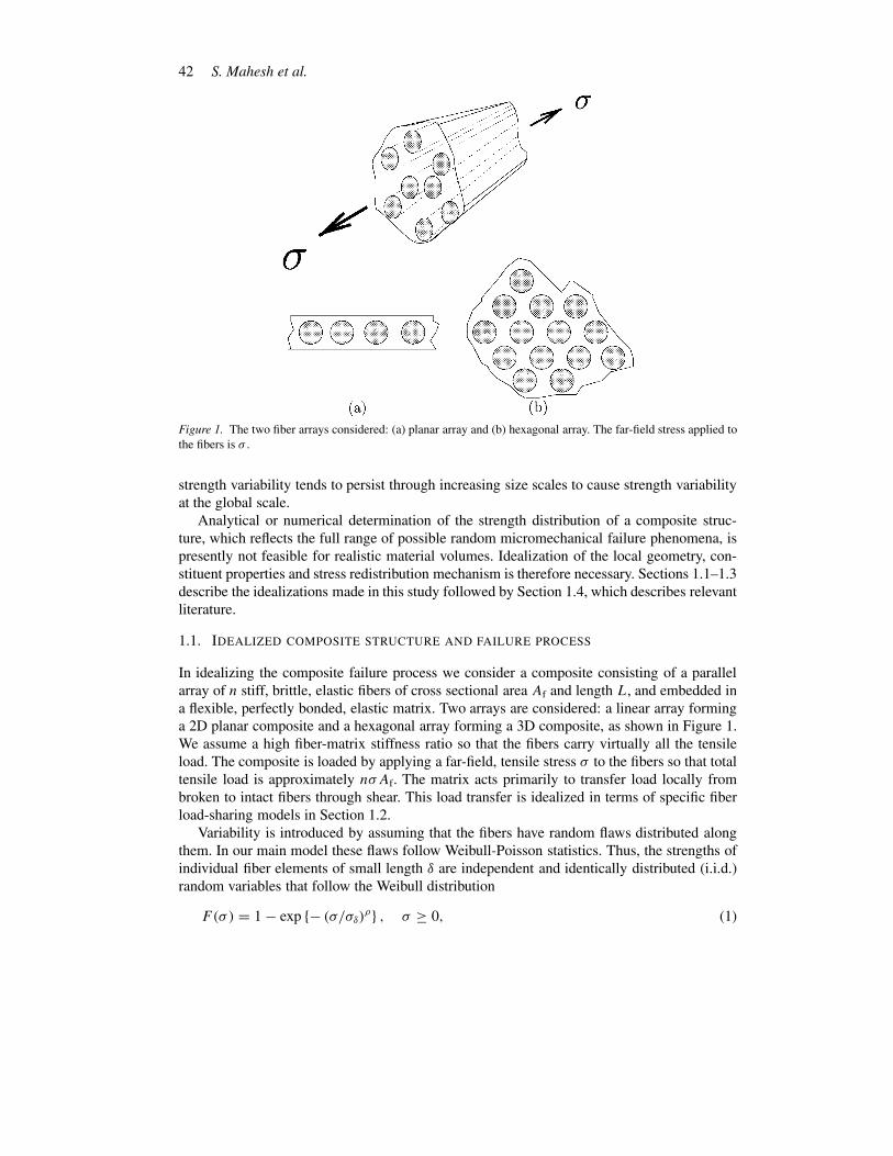
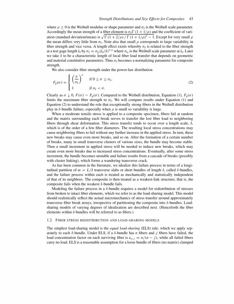
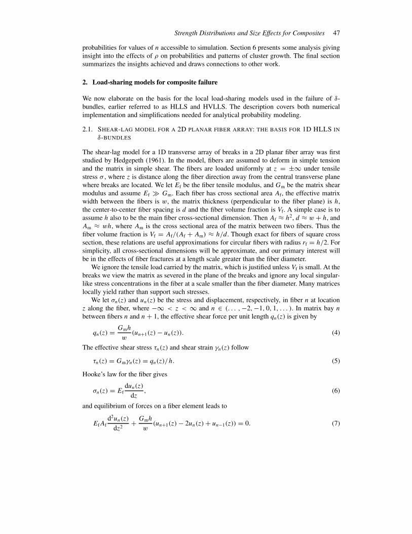
Figure 1. The two fiber arrays considered: (a) planar array and (b) hexagonal array. The far-field stress applied to
the fibers is σ .
strength variability tends to persist through increasing size scales to cause strength variability
at the global scale.
Analytical or numerical determination of the strength distribution of a composite struc-
ture, which reflects the full range of possible random micromechanical failure phenomena, is
presently not feasible for realistic material volumes. Idealization of the local geometry, con-
stituent properties and stress redistribution mechanism is therefore necessary. Sections 1.1–1.3
describe the idealizations made in this study followed by Section 1.4, which describes relevant
literature.
1.1. IDEALIZED COMPOSITE STRUCTURE AND FAILURE PROCESS
In idealizing the composite failure process we consider a composite consisting of a parallel
array of n stiff, brittle, elastic fibers of cross sectional area Af and length L, and embedded in
a flexible, perfectly bonded, elastic matrix. Two arrays are considered: a linear array forming
a 2D planar composite and a hexagonal array forming a 3D composite, as shown in Figure 1.
We assume a high fiber-matrix stiffness ratio so that the fibers carry virtually all the tensile
load. The composite is loaded by applying a far-field, tensile stress σ to the fibers so that total
tensile load is approximately nσAf. The matrix acts primarily to transfer load locally from
broken to intact fibers through shear. This load transfer is idealized in terms of specific fiber
load-sharing models in Section 1.2.
Variability is introduced by assuming that the fibers have random flaws distributed along
them. In our main model these flaws follow Weibull-Poisson statistics. Thus, the strengths of
individual fiber elements of small length δ are independent and identically distributed (i.i.d.)
random variables that follow the Weibull distribution
F(σ ) = 1 − exp {− (σ/σδ)ρ} , σ ≥ 0, (1)
Strength Distributions and Size Effects for Composites 43
where ρ ≥ 0 is the Weibull modulus or shape parameter and σδ is the Weibull scale parameter.
Accordingly the mean strength of a fiber element is σδ� (1 + 1/ρ) and the coefficient of vari-
ation (standard deviation/mean) is√
� (1 + 2/ρ) /� (1 + 1/ρ)2 − 1. Except for very small ρ
the mean differs very little from σδ . Note also that small ρ corresponds to large variability in
fiber strength and vice versa. A length effect exists whereby σδ is related to the fiber strength
at a test gage length l0 by σδ = σl0(l0/δ)1/ρ where σl0 is the Weibull scale parameter at l0. Later
we take δ to be a characteristic length of local fiber load transfer that depends on geometric
and material constitutive parameters. Thus σδ becomes a normalizing parameter for composite
strength.
We also consider fiber strength under the power-law distribution
Fp(σ ) =
(
σ
σδ
)ρ
if 0 ≤ σ ≤ σδ,
1 if σδ < σ.
(2)
Clearly as σ ↓ 0, F(σ ) ∼ Fp(σ ). Compared to the Weibull distribution, Equation (1), Fp(σ )
limits the maximum fiber strength to σδ . We will compare results under Equation (1) and
Equation (2) to understand the role that exceptionally strong fibers in the Weibull distribution
play in δ-bundle failure, especially when ρ is small so variability is large.
When a moderate tensile stress is applied to a composite specimen, fibers fail at random
and the matrix surrounding each break serves to transfer the lost fiber load to neighboring
fibers through shear deformation. This stress transfer tends to occur over a length scale, δ,
which is of the order of a few fiber diameters. The resulting local stress concentrations may
cause neighboring fibers to fail without any further increase in the applied stress. In turn, these
new breaks may cause even more breaks, and so on. After the formation of a certain number
of breaks, many in small transverse clusters of various sizes, the bundle may become stable.
Then a small increment in applied stress will be needed to induce new breaks, which may
create even more breaks due to increased stress concentrations. Eventually, after some stress
increment, the bundle becomes unstable and failure results from a cascade of breaks (possibly
with cluster linking), which forms a wandering transverse crack.
As has been common in the literature, we idealize this failure process in terms of a longi-
tudinal partition of m = L/δ transverse slabs or short bundles of length δ, called δ-bundles,
and the failure process within each is treated as mechanically and statistically independent
of that of its neighbors. The composite is then treated as a weakest-link structure; that is, the
composite fails when the weakest δ-bundle fails.
Modeling the failure process in a δ-bundle requires a model for redistribution of stresses
from broken to intact fiber elements, which we refer to as the load-sharing model. This model
should realistically reflect the actual micromechanics of stress transfer around approximately
transverse fiber break arrays, irrespective of partitioning the composite into δ-bundles. Load-
sharing models of varying degrees of idealization are described next. (Henceforth the fiber
elements within δ-bundles will be referred to as fibers.)
1.2. FIBER STRESS REDISTRIBUTION AND LOAD-SHARING MODELS
The simplest load-sharing model is the equal load-sharing (ELS) rule, which we apply sep-
arately to each δ-bundle. Under ELS, if a δ-bundle has n fibers and j fibers have failed, the
load concentration factor on each surviving fiber is κn,j = n/(n − j), while all failed fibers
carry no load. ELS is a reasonable assumption for a loose bundle of fibers (no matrix) clamped
44 S. Mahesh et al.
uniformly at each end. However, when the fibers are embedded in a matrix, the stress tends to
concentrate on the intact fibers closest to the breaks. Thus ELS is not a priori an accurate
mechanical description of stress redistribution at a composite cross-section. Nevertheless,
theoretical results under ELS will turn out to be useful in interpreting dispersed fiber failure
modes in a composite.
To account for the localized nature of fiber stress redistribution, local load-sharing (LLS)
models have been devised, the simplest of which we call the idealized local load-sharing
(ILLS) model. In a 2D planar composite, when fibers are broken within a given 1D δ-bundle,
a surviving fiber is assumed to have load concentration factor Kr = 1 + r/2 where r is the
number of contiguous failed neighbors counting on both sides. Thus a failed fiber shifts half
of its load to the closest survivor on its left and half to the one on its right; more distant
survivors receive no load. In a 3D unidirectional composite with fibers arranged in a hexag-
onal or square array, ILLS becomes 2D and load redistribution to nearest survivors requires
additional assumptions on assigning portions based on the local configuration of failed fibers.
For a large, approximately round cluster where all the lost load is redistributed onto the ring
of fibers around the circumference, Kr = 1 + D/4 where r ≈ πD2/4. Thus, D has units
corresponding to one fiber per unit cross-sectional area. In reality, ILLS is too severe, i.e.,
the stress concentration on fibers immediately adjacent to a break cluster is lower than ILLS
assumes. Also, more distant intact fibers experience some overloading due to longer range
effects.
From a micromechanics perspective, much more realistic load-sharing models for δ-bundles
can be constructed from results based on shear-lag analysis of stress transfer around single
transverse arrangements of fiber breaks in an infinite array of elastic fibers within an elastic
matrix. Such models have been developed by Hedgepeth (1961) for 2D planar fiber arrays and
by Hedgepeth and Van Dyke (1967) for 3D hexagonal or square fiber arrays. In these models
the axial fiber and matrix shear stresses can be calculated at arbitrary locations. However,
we only make use of the fiber stresses calculated along the transverse plane of the breaks,
which reduces the resulting load-sharing to 1D and 2D, respectively. Fibers within a δ-bundle
are treated as though the calculated fiber loads apply uniformly over their full lengths δ. By
these restrictions, the fiber overloading is monotonic, i.e., the load in an intact fiber will be
non-decreasing during the formation of new breaks. We refer to the 1D load-sharing model
derived from the 2D case as Hedgepeth local load-sharing (HLLS) and the 2D model from
the 3D case as Hedgepeth and Van Dyke local load-sharing (HVLLS).
In the Monte-Carlo simulations of δ-bundle failure we work with complete numerical
versions of 1D HLLS and 2D HVLLS. The stresses are calculated numerically in every intact
fiber for every arrangement of breaks that occurs in the simulations. Fundamental analyt-
ical solutions to the underlying shear-lag equations are coupled to a numerical, weighted
superposition method to treat each configuration as for example in Beyerlein et al. (1996).
In developing probability models of failure, the above approach results in serious analytical
difficulties that require further idealizations to yield simpler rules for critical configurations. In
particular, only the stresses in intact neighbors adjacent to certain idealized break clusters are
defined. In HLLS a fiber next to an isolated group of r contiguous breaks is idealized as having
load concentration factor Kr =√
1 + πr/4. In HVLLS the load concentration on the fibers
around an approximately circular cluster of diameter D is approximated as Kr =√
1 +D/π
where again r ≈ πD2/4. The square-root feature in D is consistent with a continuum fracture
mechanics viewpoint. Section 2 elaborates on their basis.
Strength Distributions and Size Effects for Composites 45
1.3. COMPOSITE STRENGTH DISTRIBUTION AND MONTE CARLO SIMULATION
APPROACH
A key quantity of interest is the distribution function Gn(σ ) for δ-bundle strength. By the
weakest link formula and chain-of-bundles assumption the strength of the composite of length
L = mδ has distribution function Hm,n(σ ) given simply by
Hm,n(σ ) = 1 − [1 −Gn(σ )]m, σ ≥ 0. (3)
The key task is to determine Gn(σ ) in terms of F(σ ) for fiber strength and the fiber load-
sharing model. We will assume periodic boundary conditions: our 1D HLLS δ-bundles will
form a tube, and under 2D HVLLS with hexagonal symmetry the simulation will be on a
rhombus patch with doubly-periodic boundary conditions.
The Monte-Carlo algorithm for simulating failure is described in detail in Mahesh et al.
(1999). In brief, to simulate the failure of a single δ-bundle, the first step is to assign numerical
strength values to each fiber as sampled from the fiber strength distribution, Equation (1) or
Equation (2). Then a load is applied to the δ-bundle, which is just enough to fail the weakest
fiber, and numerical stress redistribution is computed using either HLLS or HVLLS. If the
new fiber stresses exceed the strengths of any other fibers, then these too are failed and stress
redistribution for the new configuration is computed. This iterative process of fiber failures
and stress redistribution is continued until either stability is reached or the δ-bundle fails
catastrophically. If it becomes stable, a load increment is applied to the δ-bundle just sufficient
to fail another fiber, and the above process is repeated. Eventually, at some load increment,
a cascade of fiber failures occurs as the δ-bundle fails. The applied fiber stress triggering the
collapse is the strength of the δ-bundle.
The Monte-Carlo algorithm involves repeating the above procedure N (= 500) times for
each (n, ρ) pair, yielding N individual δ-bundle strengths. The empirical strength distribution
Gn(σ ) is constructed by plotting j/N against σ(j) for j = 1, . . . , N where σ(j) is the strength
of the j th weakest δ-bundle of the N simulated.
1.4. RESULTS AND INSIGHTS FROM PREVIOUS LITERATURE
Statistical modeling of composite failure has a long history. Pioneering work using the chain-
of-bundles framework was carried out by Gücer and Gurland (1962), Rosen (1964) and Scop
and Argon (1967), all using an ELS approach to δ-bundle failure based on the work of Daniels
(1945) and Coleman (1958). Zweben (1968), Scop and Argon (1969), Zweben and Rosen
(1970), and Argon (1974) pursued LLS approaches to δ-bundle failure, variously building
on the works of Hedgepeth (1961) and Hedgepeth and Van Dyke (1967). These works not
only initiated the discussion of dispersed versus localized cluster modes of fiber failure, but
they also served to uncover the enormous difficulties in performing probability calculations.
Harlow and Phoenix (1978a, b; 1981), Smith (1980, 1983), Smith et al. (1983) and Phoenix
and Smith (1983) simplified LLS to ILLS to capture the essence of localized fiber stress
redistribution and yet allow tractable analysis. Some of the large-ρ asymptotic results were
also developed by Batdorf (1982) and Batdorf and Ghaffarian (1982) under relaxation of the
chain-of-bundles and ILLS assumptions. They demonstrated the robustness of the chain-of-
bundles assumption as a means of capturing the crucial step of transverse evolution of failure
clusters up to instability.
More rigorous treatments for δ-bundles under 1D ILLS have also appeared. See for ex-
ample Kuo and Phoenix (1987), Harlow and Phoenix (1991), Leath and Duxbury (1994),
46 S. Mahesh et al.
and Zhang and Ding (1996). Other works for example, by Manders et al. (1982), Goda and
Phoenix (1994), Beyerlein and Phoenix (1997a, b), Curtin (1998) and Mahesh et al. (1999)
have used Monte Carlo simulation interpreted by approximate probability calculations to treat
δ-bundle failure under more realistic HLLS and HVLLS models. A full 3D failure simulation
under a special version of HVLLS for square fiber arrays and avoiding the chain-of-bundles
assumption was carried out by Landis et al. (2000). A lattice-based variation of HVLLS that
also incorporated fiber slip and pullout during failure was developed by Ibnabdeljalil and
Curtin (1997). An FEM-based, Monte Carlo model that also considered interfacial debonding
was recently developed by Goda (1999). Overviews of relevant literature have been published
by Curtin (1999) and Beyerlein (2000a).
The most important early work on ELS bundles (applied here to δ-bundles) was due to
Daniels (1945) who showed that as the number of fibers n increases, the distribution of the
strength of a bundle converges to a Gaussian or normal distribution with a fixed asymptotic
mean, and a standard deviation that decreases as 1/√n. As Smith (1982) and McCartney
and Smith (1983) showed, the convergence of Daniels’ Gaussian approximation to the true
distribution is slow with an error approximately proportional to n−1/6. By developing explicit
corrections to the mean and variance that were proportional to n−2/3, they obtained dramatic
improvements to the Gaussian approximation that worked well even for bundles with as few
as five Weibull fibers. These accurate results will form the basis for interpreting the dispersed
fiber failure mode in our Monte Carlo simulations when ρ is small.
Harlow and Phoenix (1978a, b) observed numerically that 1D ILLS δ-bundles with Weibull
fibers obey weakest-link scaling beyond a certain size n. In particular, their strength distri-
bution function, Gn(σ ) behaves such that Wn(σ ) = 1 − [1 − Gn(σ )]1/n rapidly becomes
independent of size n, converging as n → ∞ to a characteristic distribution function W(σ).
This distribution embodied the key aspects of the localized statistical failure process. Phoenix
and Smith (1983) gave a simple formula for constructing an accurate estimate of W(σ) when
fibers have modest to small strength variability (larger ρ). Beyerlein and Phoenix (1997a b)
observed from Monte Carlo simulations that δ-bundles under a full implementation of 1D
HLLS also show weakest-link behavior, and they developed an expression for W(σ) that
matched very well its empirical counterpart, Wn(σ ).
1.5. OUTLINE OF THE PAPER AND MAIN RESULTS
In the next section we describe the governing equations and main results for the shear-lag
models for fiber breaks in planar and hexagonal fiber arrays. The former forms the basis for
1D HLLS and the latter for 2D HVLLS used in Sections 3 and 4. Section 3 summarizes the
Monte-Carlo simulation results using the framework in Mahesh et al. (1999), and makes the
connection between the dominant failure mode in a δ-bundle, i.e., cluster growth for large
ρ and dispersed failure for small ρ, and the qualitative behavior of its strength distribution.
In Section 4, we study the cluster growth failure mode and derive results for the distribution
function for composite strength in terms of a characteristic distribution function W(σ) for
which we develop closed-form approximations. We also develop results under the power-law
distribution of fiber strength and through comparison to the Weibull case, as ρ decreases, we
gain insight into the effects that a few extremely strong fibers have on the results. We also
develop expressions for the critical cluster size and size effect for composite strength. Sec-
tion 5 focuses on the dispersed failure mode observed in the HVLLS and HLLS simulations
for small ρ, and uses results on ELS δ-bundles to form accurate approximations to the failure
Strength Distributions and Size Effects for Composites 47
probabilities for values of n accessible to simulation. Section 6 presents some analysis giving
insight into the effects of ρ on probabilities and patterns of cluster growth. The final section
summarizes the insights achieved and draws connections to other work.
2. Load-sharing models for composite failure
We now elaborate on the basis for the local load-sharing models used in the failure of δ-
bundles, earlier referred to as HLLS and HVLLS. The description covers both numerical
implementation and simplifications needed for analytical probability modeling.
2.1. SHEAR-LAG MODEL FOR A 2D PLANAR FIBER ARRAY: THE BASIS FOR 1D HLLS IN
δ-BUNDLES
The shear-lag model for a 1D transverse array of breaks in a 2D planar fiber array was first
studied by Hedgepeth (1961). In the model, fibers are assumed to deform in simple tension
and the matrix in simple shear. The fibers are loaded uniformly at z = ±∞ under tensile
stress σ , where z is distance along the fiber direction away from the central transverse plane
where breaks are located. We let Ef be the fiber tensile modulus, and Gm be the matrix shear
modulus and assume Ef � Gm. Each fiber has cross sectional area Af, the effective matrix
width between the fibers is w, the matrix thickness (perpendicular to the fiber plane) is h,
the center-to-center fiber spacing is d and the fiber volume fraction is Vf. A simple case is to
assume h also to be the main fiber cross-sectional dimension. Then Af ≈ h2, d ≈ w + h, and
Am ≈ wh, where Am is the cross sectional area of the matrix between two fibers. Thus the
fiber volume fraction is Vf = Af/(Af + Am) ≈ h/d. Though exact for fibers of square cross
section, these relations are useful approximations for circular fibers with radius rf = h/2. For
simplicity, all cross-sectional dimensions will be approximate, and our primary interest will
be in the effects of fiber fractures at a length scale greater than the fiber diameter.
We ignore the tensile load carried by the matrix, which is justified unless Vf is small. At the
breaks we view the matrix as severed in the plane of the breaks and ignore any local singular-
like stress concentrations in the fiber at a scale smaller than the fiber diameter. Many matrices
locally yield rather than support such stresses.
We let σn(z) and un(z) be the stress and displacement, respectively, in fiber n at location
z along the fiber, where −∞ < z < ∞ and n ∈ (. . . ,−2,−1, 0, 1, . . . ). In matrix bay n
between fibers n and n+ 1, the effective shear force per unit length qn(z) is given by
qn(z) =Gmh
w(un+1(z)− un(z)). (4)
The effective shear stress τn(z) and shear strain γn(z) follow
τn(z) = Gmγn(z) = qn(z)/h. (5)
Hooke’s law for the fiber gives
σn(z) = Ef
dun(z)
dz, (6)
and equilibrium of forces on a fiber element leads to
EfAf
d2un(z)
dz2+ Gmh
w(un+1(z)− 2un(z)+ un−1(z)) = 0. (7)
48 S. Mahesh et al.
The boundary conditions are σn(z = ±∞) = σ for all fibers, σn(0) = 0 for the r fibers
assumed to be broken on the z = 0 plane and un(z) = 0 for all intact fibers. We normalize the
various quantities above using
Pn = σn/σ,
Un = (un/δ)(Ef/σ ),
Tn = (hδ/Af)(τn/σ ),
�n = Un+1 − Un = (γnGm/σ )(hδ/Af),
ξ = z/δ,
(8)
where δ is the length scale of load transfer given by
δ =√
(EfAfw)/(Gmh) =√
Af(Ef/Gm)(w/h). (9)
These normalizations yield a non-dimensional Hooke’s law
Pn(ξ) =dUn(ξ)
dξ, (10)
and a non-dimensional system of equations
d2Un(ξ)
dξ 2+ Un+1(ξ)− 2Un(ξ)+ Un−1(ξ) = 0, (11)
with normalized boundary conditions
Pn(±∞) = 1, −∞ < n < ∞,
Pn(0) = 0, on all r broken fibers,
Un(0) = 0, for all other fibers.
(12)
For a single break at n = 0 and z = 0 this set of equations can be solved for all z
using discrete Fourier transforms. This leads to influence functions for a single break’s effect
on stress and displacements at all fiber and matrix locations. An arbitrary array of multiple
breaks lying within a single plane can be handled using a superposition of influence functions
translated to the actual break locations and weighted to satisfy the boundary conditions. This
operation requires numerically solving an r × r matrix equation where r is the number of
breaks1 . In the failure simulations, we use this method to numerically calculate the fiber loads
for all break arrays. A similar approach was used in Beyerlein et al. (1996) and Beyerlein and
Phoenix (1997a, b). This constitutes the 1D load-sharing model called HLLS.
In the probability analysis for 1D HLLS under larger ρ, we use accurate approximations to
the load concentrations due to an isolated cluster of r contiguous fiber breaks in a single plane,
or r-cluster. Specifically we want the peak load concentration factor (at the z = 0 plane) on
the nearest neighbor, denoted Kr . We also want the load concentration factor Kr,s on fiber
number s ahead of an r-cluster. Some results due to Hedgepeth (1961) and Hikami and Chou
(1990) are reviewed in Beyerlein et al. (1996) and approximations were developed there using
Stirling’s formula. The approximations
1This method works for the more general problem in which the breaks do not lie within a single plane (Beyerlein
et al., 1996). In that case numerical integration is required in evaluating the influence functions. In our case of
aligned breaks the influence functions are simple expressions.
Strength Distributions and Size Effects for Composites 49
Kr ≈√
πr
4+ 1 (13)
and
Kr,s ≈ Kr
√
1
π(s − 1)+ 1, (14)
are minor improvements on theirs, which are extremely accurate even for small r. For larger
clusters the latter result is only useful for s within about r/4 of the cluster edge, at which
point the stress concentration reaches the far-field value, unity, as seen in Beyerlein et al.
(1996). Note also that for the fibers sub-adjacent to the last break of a large r-cluster, the load
concentration drops to about one-half.
2.2. SHEAR-LAG MODEL FOR A 3D HEXAGONAL FIBER ARRAY: THE BASIS FOR 2D
HVLLS IN δ-BUNDLES
In a 3D hexagonal fiber array, as considered by Hedgepeth and Van Dyke (1967) and shown in
Figure 1, similar ideas as above apply. The fibers are identified by the index pair, (m, n) cor-
responding to axes in the transverse plane with included angle π/3 radians. All displacement
and stress quantities have subscript (m, n) to replace n in the planar case and the normaliza-
tions are the same. The main change is that the non-dimensional differential equation for the
dimensional displacement u(m,n) of fiber (m, n) becomes
d2U(m,n)(ξ)
dξ 2+
(
U(m+1,n)(ξ)+ U(m,n+1)(ξ)+ U(m−1,n)(ξ)+ U(m,n−1)(ξ)
+ U(m+1,n−1)(ξ)+ U(m−1,n+1)(ξ)− 6U(m,n)(ξ))
= 0.
(15)
Thus, six inter-fiber couplings exist for each fiber instead of two as in a planar array. The
boundary conditions are similar to those given by Equation (12) except the break array is 2D.
The numerical implementation in calculating the fiber stresses is also similar. This constitutes
the 2D load-sharing model called HVLLS.
In the probability analysis for 2D HVLLS and large ρ, we use accurate approximations
to the load concentrations due to an isolated cluster of r contiguous breaks in a single plane,
or r-cluster, which is roughly penny-shaped. First we define an effective fiber spacing d and
a dimensionless cluster diameter D. We chose d so that there is one fiber per unit cross-
sectional area. In a hexagonal array one fiber and matrix unit occupies area√
3d ′2/2, where
d ′ is the center-to-center fiber spacing, so d = (4√
3/√
2)d ′ ≈ 0.9306d ′. We define D such
that r = πD2/4, so the effective cluster diameter is Dd. The fibers surrounding the r-cluster
are subjected to the effective stress concentration
Kr ≈√
D
π+ 1 =
√
2√r
π3/2+ 1. (16)
For the decay of the stress concentration with distance, we find
Kr,s ≈Kr√
π(s − 1)+ 1, (17)
50 S. Mahesh et al.
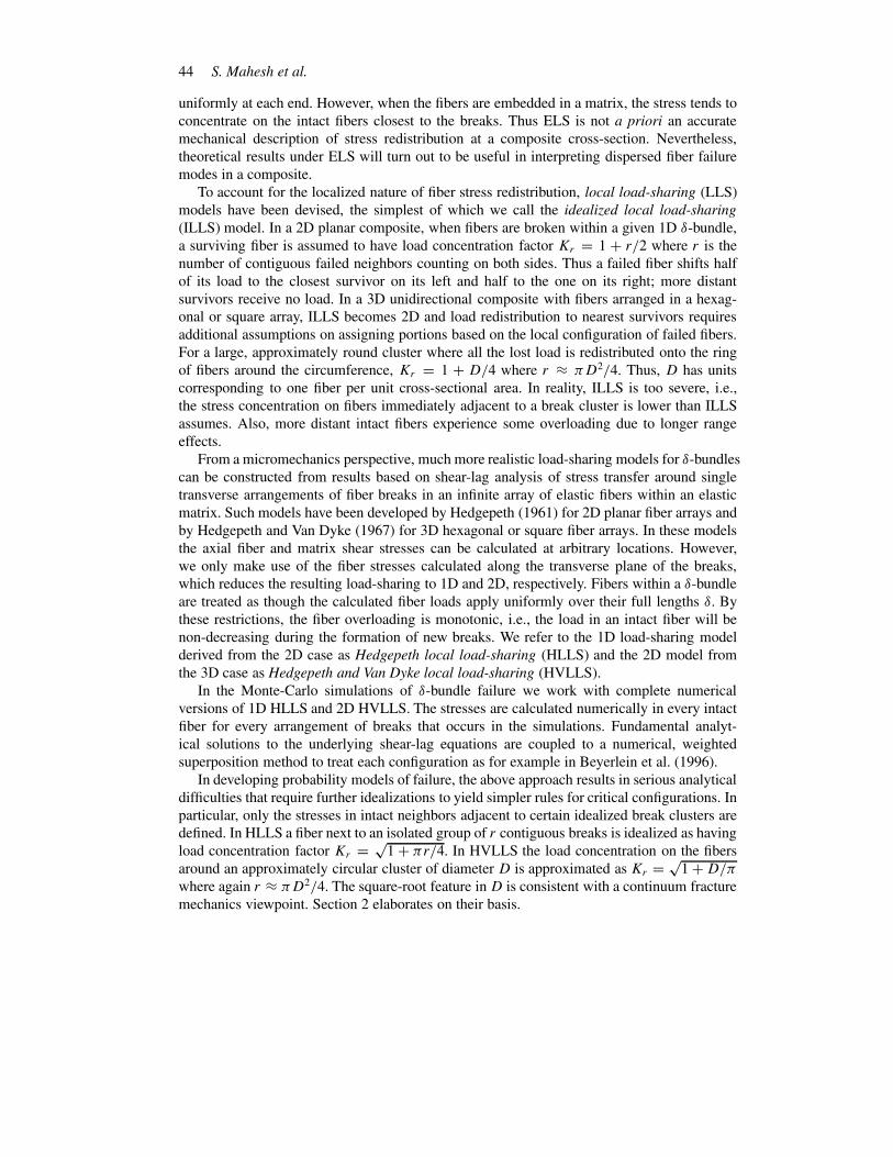
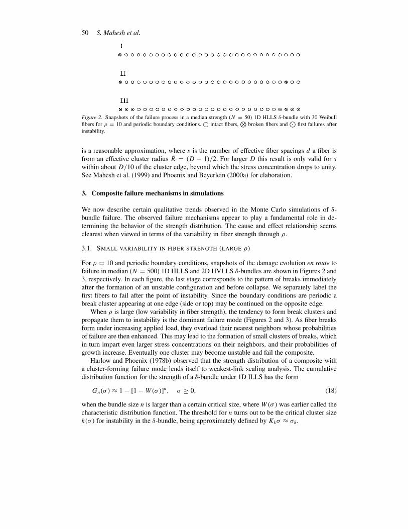
Figure 2. Snapshots of the failure process in a median strength (N = 50) 1D HLLS δ-bundle with 30 Weibull
fibers for ρ = 10 and periodic boundary conditions. © intact fibers,⊗
broken fibers and⊙
first failures after
instability.
is a reasonable approximation, where s is the number of effective fiber spacings d a fiber is
from an effective cluster radius R = (D − 1)/2. For larger D this result is only valid for s
within about D/10 of the cluster edge, beyond which the stress concentration drops to unity.
See Mahesh et al. (1999) and Phoenix and Beyerlein (2000a) for elaboration.
3. Composite failure mechanisms in simulations
We now describe certain qualitative trends observed in the Monte Carlo simulations of δ-
bundle failure. The observed failure mechanisms appear to play a fundamental role in de-
termining the behavior of the strength distribution. The cause and effect relationship seems
clearest when viewed in terms of the variability in fiber strength through ρ.
3.1. SMALL VARIABILITY IN FIBER STRENGTH (LARGE ρ)
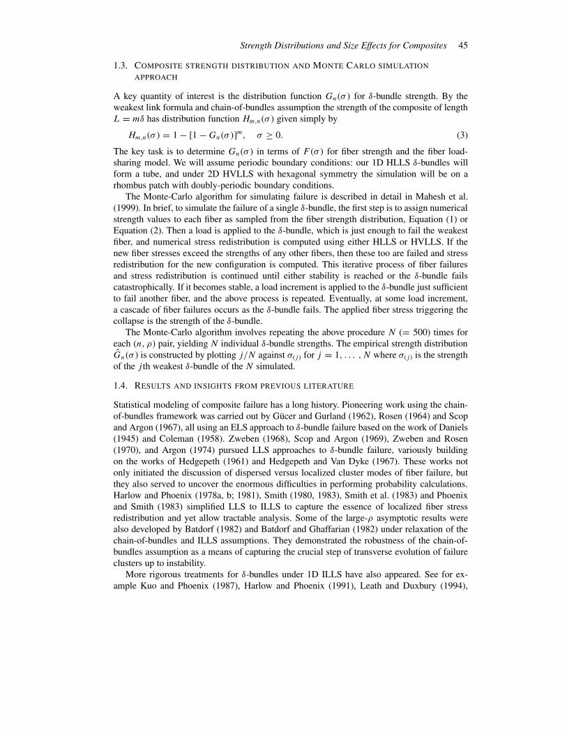
For ρ = 10 and periodic boundary conditions, snapshots of the damage evolution en route to
failure in median (N = 500) 1D HLLS and 2D HVLLS δ-bundles are shown in Figures 2 and
3, respectively. In each figure, the last stage corresponds to the pattern of breaks immediately
after the formation of an unstable configuration and before collapse. We separately label the
first fibers to fail after the point of instability. Since the boundary conditions are periodic a
break cluster appearing at one edge (side or top) may be continued on the opposite edge.
When ρ is large (low variability in fiber strength), the tendency to form break clusters and
propagate them to instability is the dominant failure mode (Figures 2 and 3). As fiber breaks
form under increasing applied load, they overload their nearest neighbors whose probabilities
of failure are then enhanced. This may lead to the formation of small clusters of breaks, which
in turn impart even larger stress concentrations on their neighbors, and their probabilities of
growth increase. Eventually one cluster may become unstable and fail the composite.
Harlow and Phoenix (1978b) observed that the strength distribution of a composite with
a cluster-forming failure mode lends itself to weakest-link scaling analysis. The cumulative
distribution function for the strength of a δ-bundle under 1D ILLS has the form
Gn(σ ) ≈ 1 − [1 −W(σ)]n, σ ≥ 0, (18)
when the bundle size n is larger than a certain critical size, where W(σ) was earlier called the
characteristic distribution function. The threshold for n turns out to be the critical cluster size
k(σ ) for instability in the δ-bundle, being approximately defined by Kkσ ≈ σδ.
Strength Distributions and Size Effects for Composites 51
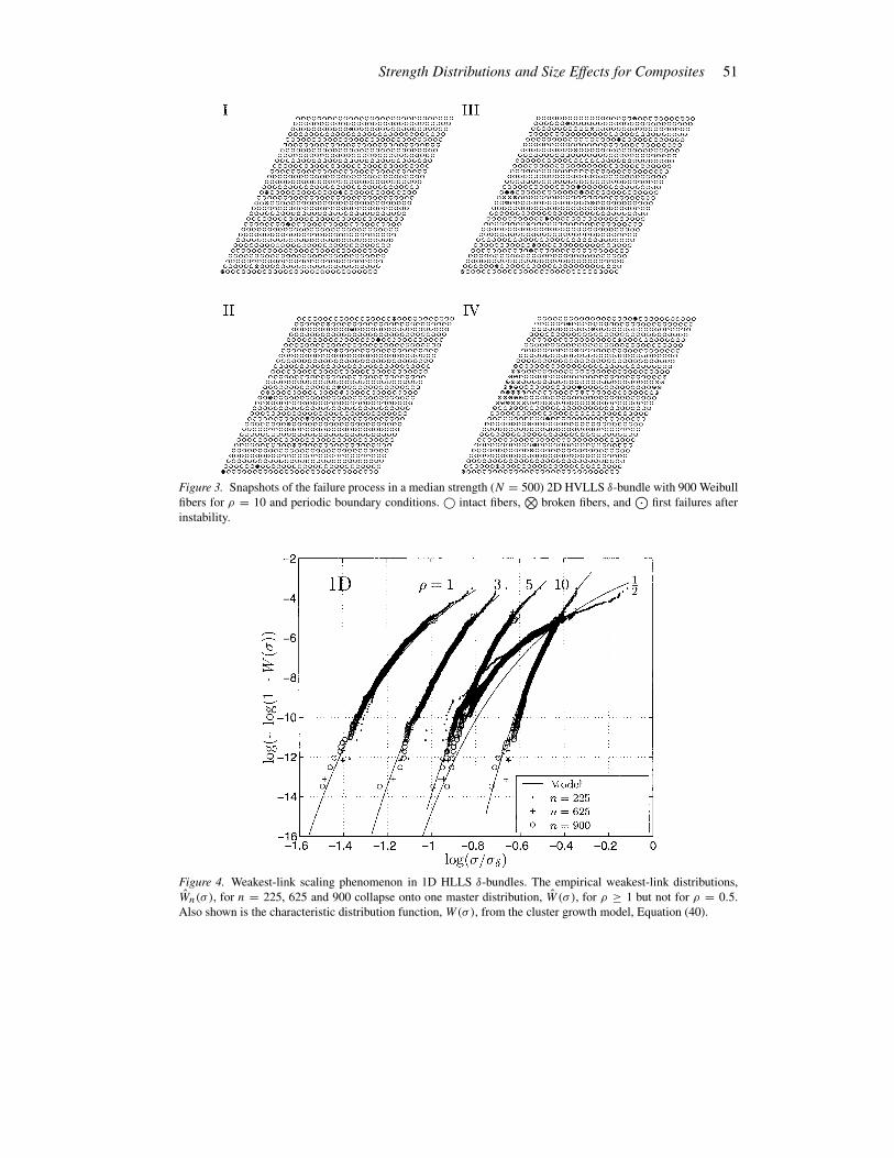
Figure 3. Snapshots of the failure process in a median strength (N = 500) 2D HVLLS δ-bundle with 900 Weibull
fibers for ρ = 10 and periodic boundary conditions. © intact fibers,⊗
broken fibers, and⊙
first failures after
instability.
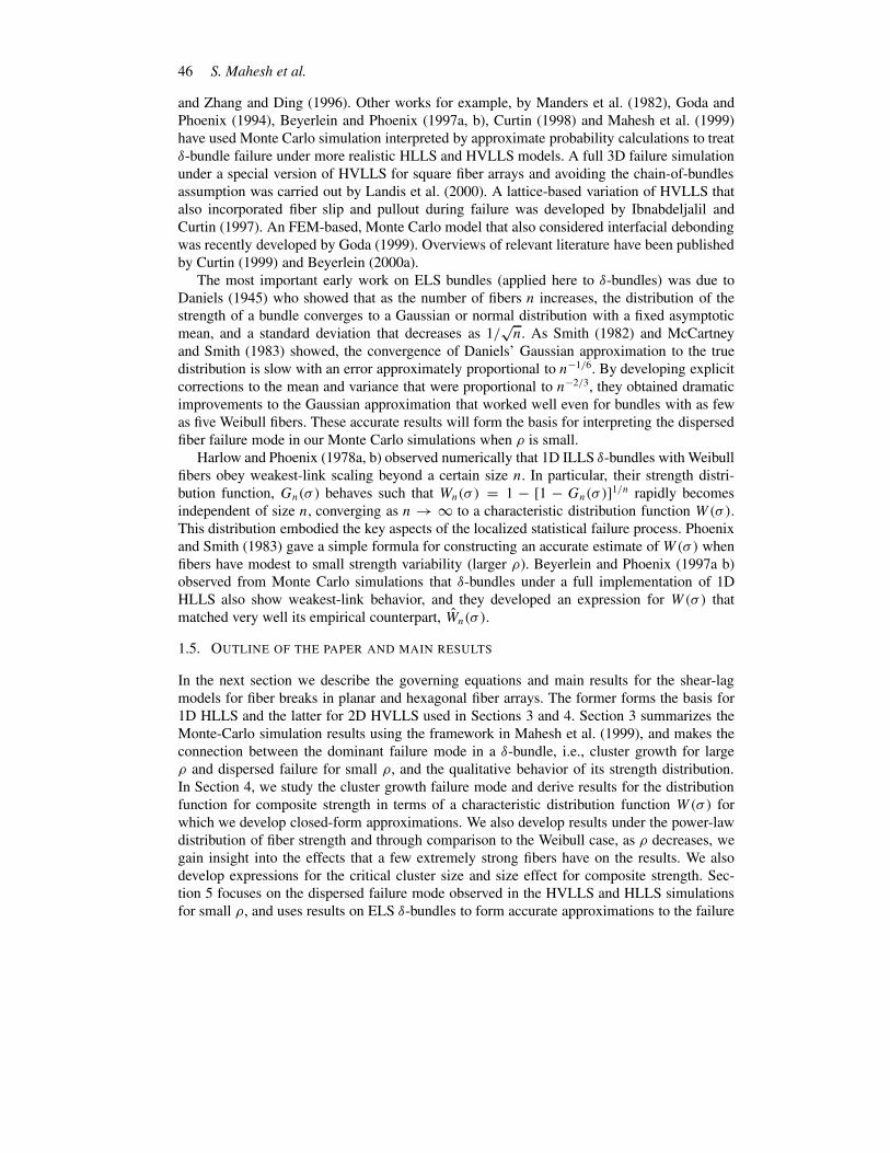
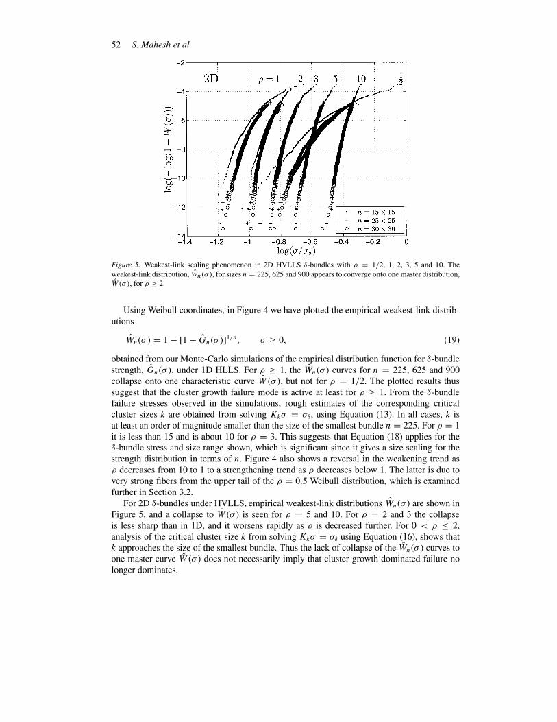
Figure 4. Weakest-link scaling phenomenon in 1D HLLS δ-bundles. The empirical weakest-link distributions,
Wn(σ ), for n = 225, 625 and 900 collapse onto one master distribution, W (σ ), for ρ ≥ 1 but not for ρ = 0.5.
Also shown is the characteristic distribution function, W(σ), from the cluster growth model, Equation (40).
52 S. Mahesh et al.
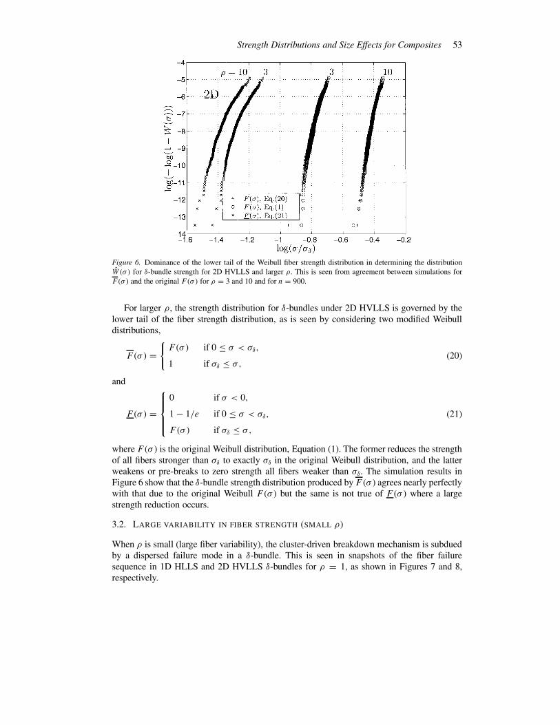
Figure 5. Weakest-link scaling phenomenon in 2D HVLLS δ-bundles with ρ = 1/2, 1, 2, 3, 5 and 10. The
weakest-link distribution, Wn(σ ), for sizes n = 225, 625 and 900 appears to converge onto one master distribution,
W(σ ), for ρ ≥ 2.
Using Weibull coordinates, in Figure 4 we have plotted the empirical weakest-link distrib-
utions
Wn(σ ) = 1 − [1 − Gn(σ )]1/n, σ ≥ 0, (19)
obtained from our Monte-Carlo simulations of the empirical distribution function for δ-bundle
strength, Gn(σ ), under 1D HLLS. For ρ ≥ 1, the Wn(σ ) curves for n = 225, 625 and 900
collapse onto one characteristic curve W (σ ), but not for ρ = 1/2. The plotted results thus
suggest that the cluster growth failure mode is active at least for ρ ≥ 1. From the δ-bundle
failure stresses observed in the simulations, rough estimates of the corresponding critical
cluster sizes k are obtained from solving Kkσ = σδ, using Equation (13). In all cases, k is
at least an order of magnitude smaller than the size of the smallest bundle n = 225. For ρ = 1
it is less than 15 and is about 10 for ρ = 3. This suggests that Equation (18) applies for the
δ-bundle stress and size range shown, which is significant since it gives a size scaling for the
strength distribution in terms of n. Figure 4 also shows a reversal in the weakening trend as
ρ decreases from 10 to 1 to a strengthening trend as ρ decreases below 1. The latter is due to
very strong fibers from the upper tail of the ρ = 0.5 Weibull distribution, which is examined
further in Section 3.2.
For 2D δ-bundles under HVLLS, empirical weakest-link distributions Wn(σ ) are shown in
Figure 5, and a collapse to W (σ ) is seen for ρ = 5 and 10. For ρ = 2 and 3 the collapse
is less sharp than in 1D, and it worsens rapidly as ρ is decreased further. For 0 < ρ ≤ 2,
analysis of the critical cluster size k from solving Kkσ = σδ using Equation (16), shows that
k approaches the size of the smallest bundle. Thus the lack of collapse of the Wn(σ ) curves to
one master curve W (σ ) does not necessarily imply that cluster growth dominated failure no
longer dominates.
Strength Distributions and Size Effects for Composites 53
Figure 6. Dominance of the lower tail of the Weibull fiber strength distribution in determining the distribution
W(σ ) for δ-bundle strength for 2D HVLLS and larger ρ. This is seen from agreement between simulations for
F(σ) and the original F(σ) for ρ = 3 and 10 and for n = 900.
For larger ρ, the strength distribution for δ-bundles under 2D HVLLS is governed by the
lower tail of the fiber strength distribution, as is seen by considering two modified Weibull
distributions,
F(σ ) ={
F(σ ) if 0 ≤ σ < σδ,
1 if σδ ≤ σ,(20)
and
F(σ ) =
0 if σ < 0,
1 − 1/e if 0 ≤ σ < σδ,
F (σ ) if σδ ≤ σ,
(21)
where F(σ ) is the original Weibull distribution, Equation (1). The former reduces the strength
of all fibers stronger than σδ to exactly σδ in the original Weibull distribution, and the latter
weakens or pre-breaks to zero strength all fibers weaker than σδ. The simulation results in
Figure 6 show that the δ-bundle strength distribution produced by F(σ ) agrees nearly perfectly
with that due to the original Weibull F(σ ) but the same is not true of F(σ ) where a large
strength reduction occurs.
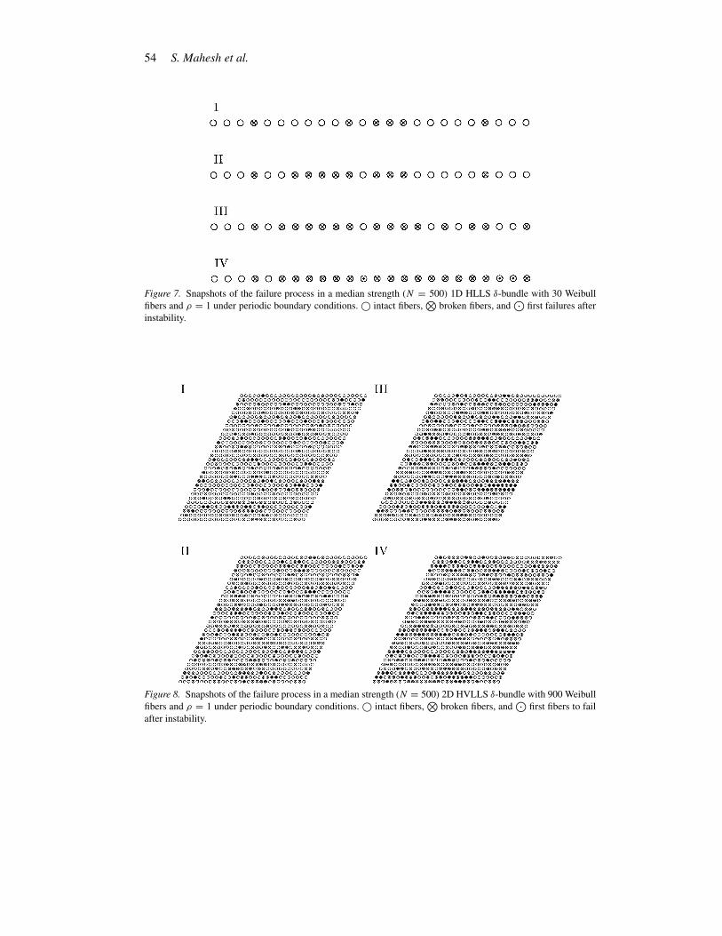
3.2. LARGE VARIABILITY IN FIBER STRENGTH (SMALL ρ)
When ρ is small (large fiber variability), the cluster-driven breakdown mechanism is subdued
by a dispersed failure mode in a δ-bundle. This is seen in snapshots of the fiber failure
sequence in 1D HLLS and 2D HVLLS δ-bundles for ρ = 1, as shown in Figures 7 and 8,
respectively.
54 S. Mahesh et al.
Figure 7. Snapshots of the failure process in a median strength (N = 500) 1D HLLS δ-bundle with 30 Weibull
fibers and ρ = 1 under periodic boundary conditions. © intact fibers,⊗
broken fibers, and⊙
first failures after
instability.
Figure 8. Snapshots of the failure process in a median strength (N = 500) 2D HVLLS δ-bundle with 900 Weibull
fibers and ρ = 1 under periodic boundary conditions. © intact fibers,⊗
broken fibers, and⊙
first fibers to fail
after instability.
Strength Distributions and Size Effects for Composites 55
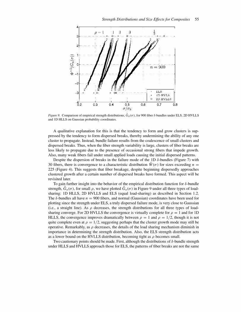
Figure 9. Comparison of empirical strength distributions, Gn(σ ), for 900 fiber δ-bundles under ELS, 2D HVLLS
and 1D HLLS on Gaussian probability coordinates.
A qualitative explanation for this is that the tendency to form and grow clusters is sup-
pressed by the tendency to form dispersed breaks, thereby undermining the ability of any one
cluster to propagate. Instead, bundle failure results from the coalescence of small clusters and
dispersed breaks. Thus, when the fiber strength variability is large, clusters of fiber breaks are
less likely to propagate due to the presence of occasional strong fibers that impede growth.
Also, many weak fibers fail under small applied loads causing the initial dispersed patterns.
Despite the dispersion of breaks in the failure mode of the 1D δ-bundles (Figure 7) with
30 fibers, there is convergence to a characteristic distribution W (σ ) for sizes exceeding n =225 (Figure 4). This suggests that fiber breakage, despite beginning dispersedly approaches
clustered growth after a certain number of dispersed breaks have formed. This aspect will be
revisited later.
To gain further insight into the behavior of the empirical distribution function for δ-bundle
strength, Gn(σ ), for small ρ, we have plotted Gn(σ ) in Figure 9 under all three types of load-
sharing: 1D HLLS, 2D HVLLS and ELS (equal load-sharing) as described in Section 1.2.
The δ-bundles all have n = 900 fibers, and normal (Gaussian) coordinates have been used for
plotting since the strength under ELS, a truly dispersed failure mode, is very close to Gaussian
(i.e., a straight line). As ρ decreases, the strength distributions for all three types of load-
sharing converge. For 2D HVLLS the convergence is virtually complete for ρ = 1 and for 1D
HLLS, the convergence improves dramatically between ρ = 1 and ρ = 1/2, though it is not
quite complete even at ρ = 1/2, suggesting perhaps that the cluster growth mode may still be
operative. Remarkably, as ρ decreases, the details of the load sharing mechanism diminish in
importance in determining the strength distribution. Also, the ELS strength distribution acts
as a lower bound on the HVLLS distribution, becoming tight as ρ becomes small.
Two cautionary points should be made. First, although the distributions of δ-bundle strength
under HLLS and HVLLS approach those for ELS, the patterns of fiber breaks are not the same
56 S. Mahesh et al.
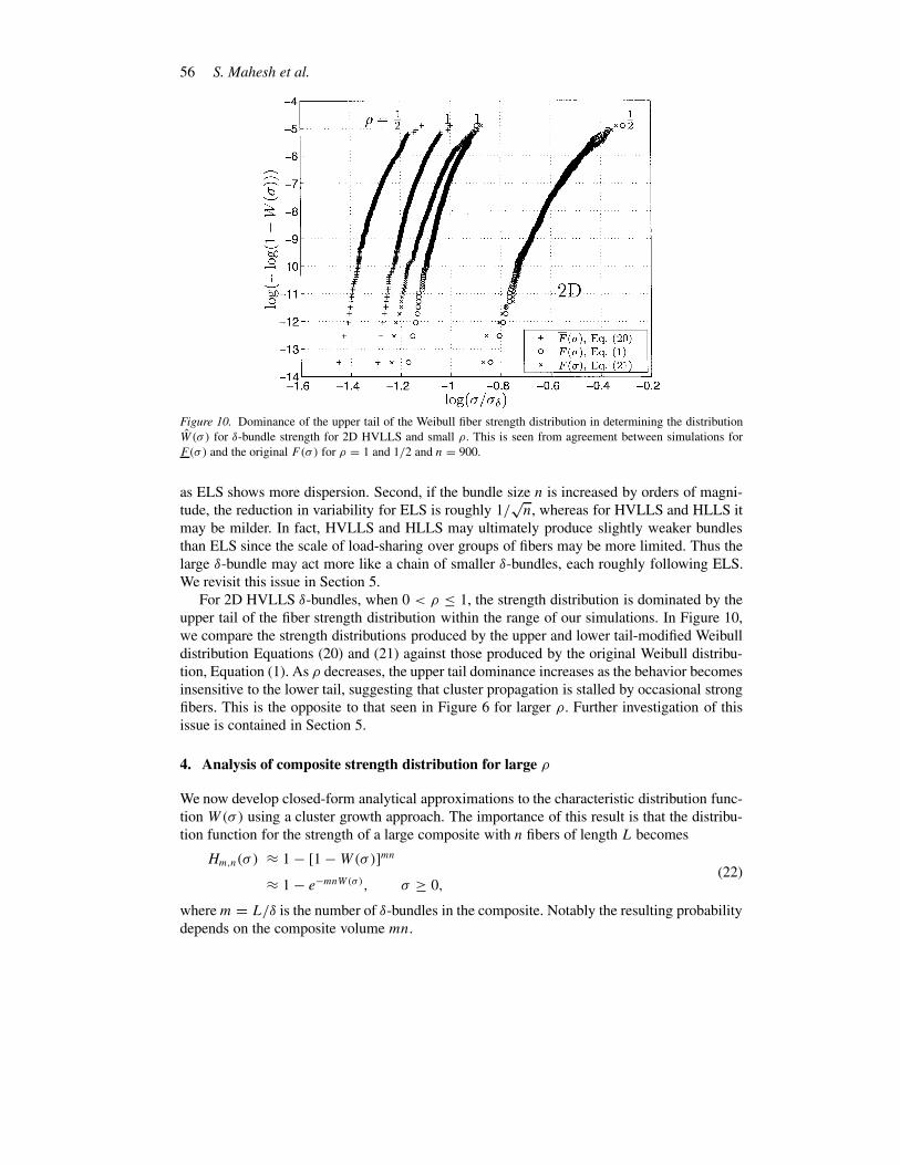
Figure 10. Dominance of the upper tail of the Weibull fiber strength distribution in determining the distribution
W(σ ) for δ-bundle strength for 2D HVLLS and small ρ. This is seen from agreement between simulations for
F(σ ) and the original F(σ) for ρ = 1 and 1/2 and n = 900.
as ELS shows more dispersion. Second, if the bundle size n is increased by orders of magni-
tude, the reduction in variability for ELS is roughly 1/√n, whereas for HVLLS and HLLS it
may be milder. In fact, HVLLS and HLLS may ultimately produce slightly weaker bundles
than ELS since the scale of load-sharing over groups of fibers may be more limited. Thus the
large δ-bundle may act more like a chain of smaller δ-bundles, each roughly following ELS.
We revisit this issue in Section 5.
For 2D HVLLS δ-bundles, when 0 < ρ ≤ 1, the strength distribution is dominated by the
upper tail of the fiber strength distribution within the range of our simulations. In Figure 10,
we compare the strength distributions produced by the upper and lower tail-modified Weibull
distribution Equations (20) and (21) against those produced by the original Weibull distribu-
tion, Equation (1). As ρ decreases, the upper tail dominance increases as the behavior becomes
insensitive to the lower tail, suggesting that cluster propagation is stalled by occasional strong
fibers. This is the opposite to that seen in Figure 6 for larger ρ. Further investigation of this
issue is contained in Section 5.
4. Analysis of composite strength distribution for large ρ
We now develop closed-form analytical approximations to the characteristic distribution func-
tion W(σ) using a cluster growth approach. The importance of this result is that the distribu-
tion function for the strength of a large composite with n fibers of length L becomes
Hm,n(σ ) ≈ 1 − [1 −W(σ)]mn
≈ 1 − e−mnW(σ), σ ≥ 0,(22)
where m = L/δ is the number of δ-bundles in the composite. Notably the resulting probability
depends on the composite volume mn.
Strength Distributions and Size Effects for Composites 57
4.1. CHARACTERISTIC DISTRIBUTION W(σ) UNDER 1D HLLS
For 1D HLLS we model δ-bundle failure as a linear cascade of fiber failures following Smith
(1980), and approximate the probability that such a cascade occurs starting with the failure
of a given fiber. The structure of such an event is that under applied stress σ , a given fiber
fails, and its two immediate neighbors then suffer stress K1σ , of which one fails. The pair of
breaks formed causes one of the two adjacent overloaded neighbors to fail under stress K2σ ,
the resulting triplet then fails one of its two overloaded neighbors under stress K3σ , and so on
until all n fibers have failed. Thus, W(σ) is approximately
Wn(σ ) ≈ F(σ ){1 − [1 − F(K1σ )]2}{1 − [1 − F(K2σ )]2} · · ·{1 − [1 − F(Kn−1σ )]2}
={
1 − exp
[
−(
σ
σδ
)ρ]} n−1∏
r=1
{
1 − exp
[
−2
(
Krσ
σδ
)ρ]}
,
(23)
where Kr is the stress concentration on the two fibers next to an r-cluster as approximated by
Equation (13), and F(σ ) is given by Equation (1).
Simplifying assumptions are made in writing Equation (23). First, only the failure of the
fibers adjacent to an r-cluster are considered. Failure of fibers further away is ignored even
though such fibers are overloaded. This is justified because, as r becomes large, the fibers
neighboring the cluster carry twice as much load as the fibers sub-adjacent to it, according to
Equation (14). Thus for large ρ, the probability of failure of a sub-adjacent fiber without the
failure of the adjacent fiber is negligible. Second, the formula assumes that fibers next to the
cluster are virgin. In other words, in evaluating the probability of failure of an overloaded fiber
at stress Krσ , the event that it survived a lower stress Kjσ , j < r is ignored. While the first
assumption decreases the calculated probability of failure relative to the true one, the second
assumption increases it. For large ρ, the errors thus committed tend to cancel.
While Equation (23) can be used directly to estimate W(σ) numerically for larger n, it is
more illuminating to have a functional form for W(σ) independent of n. When Krσ � σδ we
have
1 − exp
[
−2
(
Krσ
σδ
)ρ]
≈ 2
(
Krσ
σδ
)ρ [
1 −(
Krσ
σδ
)ρ]
. (24)
This simplification becomes inaccurate when Krσ exceeds σδ and the probability of subse-
quent failures very rapidly approaches one. To preserve accuracy in this range, we rewrite
Equation (23) as
W(σ) ≈{
(
σ
σδ
)ρ k(σ )−1∏
j=1
[
2
(
Kjσ
σδ
)ρ]}{
k(σ )−1∏
j=1
[
1 −(
Kjσ
σδ
)ρ]}
×{
∞∏
j=k(σ )
[
1 − exp
(
−2
(
Kjσ
σδ
)ρ)]}
≡{
Wk(σ )(σ )}
{.1(σ )} {.2(σ )} ,
(25)
where k(σ ) is a critical cluster size depending on σ as described shortly. Here we have
preserved the explicit dependence on k of the first quantity, which can be written as
58 S. Mahesh et al.
Wk(σ ) = 2k−1(K1K2 · · ·Kk−1)ρ
(
σ
σδ
)kρ
, (26)
and the third product .2(σ ), in Equation (25), is carried out to ∞ instead of n since the terms
rapidly converge to unity whereby the product is virtually independent of n, so we drop n as a
subscript.
One way to define k(σ ) might be to take it as the integer satisfying
F(Kk−1σ ) < 1 − 1
e≤ F(Kkσ ). (27)
This, however, leads to a discontinuous W(σ) because the 2k−1 factor in Equation (26) pre-
vents W(σ) from being continuous at exactly σ/σδ = 1/Kk . Smooth transitions, however, do
occur at certain values of σ where the right hand side of Equation (26) has the same value for
both k and k + 1, i.e., for a transition σ such that
2k−1(K1K2 · · ·Kk−1)ρ
(
σ
σδ
)kρ
= 2k(K1K2 · · ·Kk)ρ
(
σ
σδ
)(k+1)ρ
. (28)
Taking the approximation Equation (13) as the equality
Kr =√
b + r
b, (29)
we then have
σ
σδ= 2−1/ρ
Kk
= a√k + b
, (30)
where
a = 2(ρ−1)/ρ/π1/2 and b = 4/π. (31)
When σ is decreased continuously the associated k cannot increase continuously since
it takes on only integer values. If we relax this requirement and also permit k to vary con-
tinuously, we may replace σ/σδ in Equation (26) in terms of k according to Equation (30).
In addition, substituting for Kr using Equation (29) we have Wk(σ ) only as a function of k
whereby
Wk =aρ
(k + b)kρ/2
k−1∏
r=1
(r + b)ρ/2. (32)
Evaluating the product in Equation (32) yields
∏k−1r=1(r + b)ρ/2 = exp
{
ρ
2
k−1∑
r=1
log(r + b)
}
≈ exp
{
ρ
2
∫ k
1
log(u+ b) du− ρ
4
∫ k
1
1
u+ bdu
}
=(
(b + k)b+k−1/2
(b + 1)b+1/2
)ρ/2
exp
{
−ρ(k − 1)
2
}
,
(33)

Strength Distributions and Size Effects for Composites 59
so that
Wk = C(k + b)φ exp {−β(k + b)} , (34)
where
β = ρ
2, φ = ρ
(
b
2− 1
4
)
, and C = aρeβ(b+1)(1 + b)−β(b+1/2). (35)
To get a relationship between Wk and σ , we use Equation (30) relating k to σ , and upon
simplification obtain
Wk(σ )(σ ) = C(aσδ
σ
)2φ
exp
{
−β(aσδ
σ
)2}
. (36)
Next we approximate .1(σ ) in Equation (25). Using Equation (30) we obtain
.1(σ ) =k(σ )∏
j=1
[
1 −(
Kjσ
σδ
)ρ]
≈ exp
{
−k(σ )∑
j=1
(
Kjσ
σδ
)ρ}
≈ exp
{
−1
2
∫ k(σ )
0
(b + u)ρ/2
(
σ
aσδ
)ρ
du
}
≈ exp
{
−(aσδ
σ
)2 2
2(ρ + 2)
[
1 − b(ρ+2)/2
(
σ
aσδ
)ρ+2]}
.
(37)
Finally we evaluate .2(σ ), the third product in Equation (25), which is the probability of
cluster stalling. Upon using Equation (30) we obtain
.2(σ ) =∞∏
j=k(σ )
[
1 − exp
{
−2
(
Kjσ
σδ
)ρ}]
≈ exp
{
−∞∑
j=k(σ )
exp
{
−2
(
Kjσ
σδ
)ρ}}
≈ exp
{
−∫ ∞
k(σ )
exp
{
−(b + u)ρ/2
(
σ
aσδ
)ρ}
du
}
= exp
{
− 2
ρ�(2/ρ, 1)
(aσδ
σ
)2}
,
(38)
where
�(p, 1) =∫ ∞
1
e−uup−1 du (39)
is the incomplete gamma function.
Substituting Equations (36)–(38) into Equation (25) and keeping the dominant term in
Equation (37), we obtain the key result
60 S. Mahesh et al.
W(σ) ≈ C(aσδ
σ
)2φ
exp
{
−Bβ(aσδ
σ
)2}
, (40)
where
B = 1 +(
2
ρ
)2 [ρ
2(ρ + 2)+ �(2/ρ, 1)
]
, (41)
and all other constants are as defined in Equations (31) and (35). Note that as ρ decreases
below 2, B begins to grow rapidly, lowering W(σ).
Since there are n fibers in a δ-bundle, a cascade can originate from any one of them, and
these events are taken as being statistically independent. This results in the approximation
Equation (18), and using Equation (3) gives Hm,n(σ ) for the full composite as given by
Equation (22).
To investigate its success, in Figure 4 we compare W(σ) of Equation (40) to W (σ ), which
results from the convergence of the Monte Carlo simulated Wn(σ ) of Equation (19) with
increasing n. No adjustable parameters are involved. For ρ = 1, 3, 5 and 10, the calculated
and simulated distributions are in remarkable agreement. For ρ = 0.5 the agreement suddenly
weakens where no n-independent W (σ ) quite emerges. This lack of agreement may simply
mean that the bundle sizes are too small, but nevertheless, it is consistent with our earlier
observations in Figure 9 where the distribution Gn(σ ) for δ-bundle strength was close to that
for ELS, which has a dispersed fiber failure mode. The value ρ = 2 does not emerge as having
a dominating effect. Surprisingly the model seems to apply well for ρ = 1, and Figure 4 does
not rule out its application for ρ = 1/2 either. This issue is revisited in Section 5.
4.2. SIZE EFFECTS FOR CRITICAL CLUSTER AND COMPOSITE STRENGTH UNDER HLLS
We next examine the size effect for the characteristic composite strength. That is, for fixed
probability of failure p, we ask how the composite strength for the p-th quantile scales in
terms of number of fibers n and length L = mδ where m is the number of δ-bundles in the
composite. We take p = 1 − 1/e = 0.632, which would correspond to the Weibull scale
parameter for composite strength in a Weibull approximation to Hm,n(σ ). We examine the
dependence of the critical cluster size on n at failure probability level p, and want to know
the size of the critical cluster at the point where it becomes unstable. Extending these results
to the full composite is simply a matter of replacing n by mn.
We know that
Gn(σ ) ≈ 1 − [1 −W(σ)]n ≈ 1 − e−nW(σ). (42)
Equating this further to 1 − e−1, we find that the characteristic δ-bundle strength, denoted
σ ∗c , is the stress σ solving W(σ) = 1/n where W(σ) is given by Equation (40). While this
equation can be inverted asymptotically to get σ ∗c , it turns out to be useful to think also in
terms of a critical cluster size k∗ associated with failure probability p. This is obtained by
setting Wk = 1/n in Equation (34), that is, k∗ must solve
(k∗ + b)−φeβ(k∗+b) = nC. (43)
To obtain an explicit relation between k∗ and n, we observe that
−φ log(k∗ + b)+ β(k∗ + b) = log(nC). (44)
Strength Distributions and Size Effects for Composites 61
Substituting k∗ + b = (1 + ε) log(nC)/β and using log(1 + ε) ≈ ε gives the critical cluster
size k∗ for a δ-bundle approximately as
k∗ + b = (1 + ε)log(nC)
β, (45)
where
ε ≈ φ {log[log(nC)] − log(β)}log(nC)− φ
, (46)
and log is the Napierian logarithm. To obtain an integer valued k∗, one must round up the
k∗ from Equation (45) to the next largest integer. To obtain k∗ for the full composite simply
replace n by mn in Equation (45).
To obtain the characteristic strength σ ∗c of a δ-bundle we first use Equation (30) to recast
Equation (45) in terms of σ , yielding the critical stress
σ ∗ = aσδ
√
β
log(nC)(1 + ε). (47)
This expression, however, does not account for the crack stalling probability .2(σ ). It can
be interpreted as the stress associated with f ormation of a cluster of critical size k∗ where
the probability of further propagation becomes likely but not guaranteed to be catastrophic.
Including .2(σ ) as well yields the characteristic δ-bundle strength
σ ∗c = aσδ
√
Bβ
log(nC)(1 + ε(Bβ)), (48)
where ε(Bβ) is Equation (46) but with β replaced by Bβ. To obtain the characteristic com-
posite strength, replace n by mn in Equation (48).
Figure 11 shows plots of the characteristic strength σ ∗c versus δ-bundle size n based on
Equation (48). The agreement is good even for ρ = 1/2, which did not show failure by cluster
growth over this range of n.
4.3. CHARACTERISTIC DISTRIBUTION W(σ) UNDER 2D HVLLS
The approach taken to approximate W(σ) for 2D HVLLS is similar to that in 1D HLLS
except there are many more possible break cluster geometries and sequences of fiber failures
to introduce complications. For a δ-bundle loaded at stress σ , we again model the cascade
event defining W(σ) as the formation of a break cluster at a given location, which then grows
to instability. Intermediate steps involve clusters of increasing size, and for a cluster of r
breaks an important quantity is Nr , the number of neighboring fibers that are at highest risk
of failure. Initially we follow Smith et al. (1983) and take this to be the number of severely
overloaded, immediate neighbors.
An approximation to the probability of formation of such a cluster is calculated following
the approach of Smith et al. (1983). First is the failure of a given fiber under stress σ , followed
by the failure of one of its N1 = 6 equally overloaded neighbors under stress K1σ . The
resulting pair of fiber breaks has eight intact neighbors of which only N2 = 2 are severely
overloaded under stress K2σ . Next is the failure of one of these, to form a break triplet with
N3 = 3 severely overloaded neighbors, of which one fails, and so on. The critical event is thus
62 S. Mahesh et al.
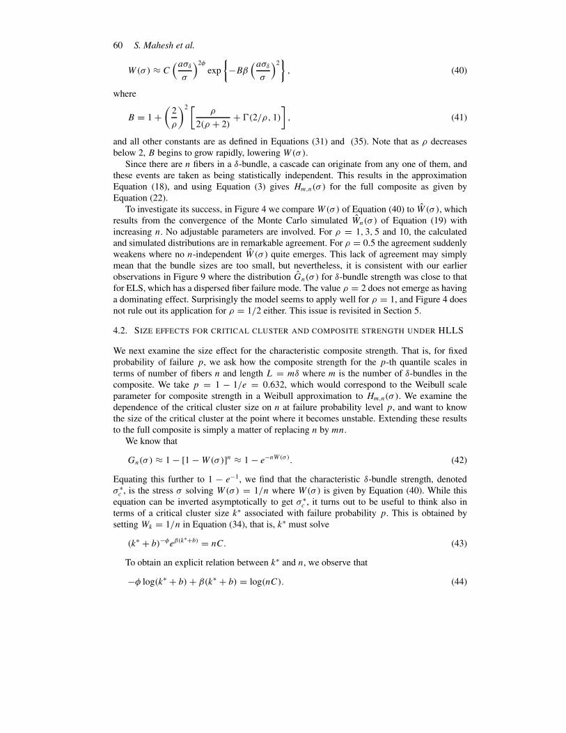
Figure 11. Comparison of Equation (47) with size effect predicted from the simulated empirical strength
distributions of a 900-fiber δ-bundle under 1D HLLS.
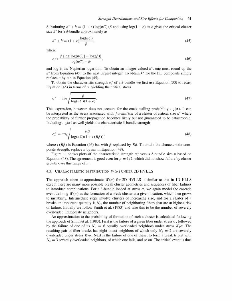
Figure 12. One possible sequence of tight cluster growth to 10 fiber breaks in a hexagonal fiber array. The numbers
(r = 1, 2, . . . , 10) indicate break sequence. Also included are the associated stress concentrations Kr computed
under HVLLS, where K9 causes break 10.
the evolution of a growing ‘tight’ r-cluster with each added break being the failure of one of
the Nr severely overloaded fibers surrounding it under Kr as shown in Figure 12. Continuing
this process, we arrive at the general form
Wn(σ ) ≈ F(σ ){1 − [1 − F(K1σ )]N1}×{1 − [1 − F(K2σ )]N2} · · · {1 − [1 − F(Kn−1σ )]Nn−1}.
(49)
Strength Distributions and Size Effects for Composites 63
To derive useful approximations, we need simple analytical forms for Kr and Nr . For a
tight circular cluster of r breaks, its diameter D was defined by πD2/4 = r, so for Kr we
will use the approximation Equation (16). For Nr , we note that the number of intact neighbors
surrounding this r-cluster is approximately its circumference, πD =√
4πr , but we just saw
that some are much more overloaded than others with the true Kr in Figure 12 typically a
little larger than that predicted by Equation (16), whereas the others are smaller. Thus, except
for very small ρ, these few neighbors are at higher risk of failure, but overall, the risk of
subsequent failures may or may not be enhanced compared to using Kr of Equation (16) and
Nr as all the circumference. To provide flexibility in both modeling and comparing to later
simulations, we introduce a simple power law to represent the effective number of neighbors
at high risk, i.e.,
Nr = ηrγ , (50)
where η and γ are parameters that satisfy η > 0 and γ ≥ 0 and possibly depend on ρ. By
taking η =√
4π ≈ 3.5 and γ = 1/2, Nr becomes the circumference.
In comparing theory to simulations, a good fit for small ρ will require γ in Nr to be
much smaller than 1/2. In fact, γ quickly approaches zero and η approaches 6 as ρ decreases
below about 5, so that Nr approaches 6, the number of neighbors to a single break. This
surprising result suggests that, as the variability in fiber strength becomes large, the total
number of neighbors to an r-cluster becomes irrelevant in our approximation, Equation (49),
for calculating W(σ). In this approximation, use of F(Krσ ) for all Nr fibers means they are
all treated as ‘virgin’ fibers. In reality, however, when a fiber fails next to a large r-cluster,
except for the few fibers near this new break, the other fibers around the cluster will already
have survived previous high load concentrations and will be subjected only to a relatively
small load increment. Thus, their risks of failure are much smaller than those of the few fibers
nearest the new break. This aspect turns out to be increasingly important as ρ decreases and
clusters become large, and will lead to an explanation for why the above power form for Nr is
needed and associated behavior of γ and η is observed.
Proceeding with the derivation of W(σ), we apply approximations as in Section 4.1 and
rewrite Equation (49) as
W(σ) ≈{
(
σ
σδ
)ρ k(σ )−1∏
j=1
[
Nj
(
Kjσ
σδ
)ρ]}{
k(σ )−1∏
j=1
[
1 − Nj
2
(
Kjσ
σδ
)ρ]}
×{
∞∏
j=k(σ )
[
1 − exp
(
−Nj
(
Kjσ
σδ
)ρ)]}
≡{
Wk(σ )(σ )}
{.1(σ )} {.2(σ )} .
(51)
Again the explicit dependence on k in the first product Wk(σ )(σ ) is retained, and it may be
written as
Wk(σ ) = N1N2 · · ·Nk−1(K1K2 · · ·Kk−1)ρ
(
σ
σδ
)kρ
. (52)
As in the case of 1D, we relate σ to k by setting Wk(σ ) = Wk+1(σ ). Doing so and recalling
Equation (16) for Kr , which we rewrite as
Kr =
√√r + b
b, (53)
64 S. Mahesh et al.
we obtain
σ
σδ= ak−γ /ρ(
√k + b)−1/2, (54)
where
a =√b/η1/ρ and b = π3/2/2. (55)
Using Equations (50), (53) and (54) in Equation (52) and simplifying we obtain
Wk =[(k − 1)!]γ
∏k−1j=0(
√j + b)ρ/2
ηkkγ (√k + b)kρ/2
. (56)
We can evaluate Equation (56) as follows: by Stirling’s formula,
(k − 1)! ≈√
2πkk−1/2e−k . (57)
Also,
k−1∏
j=0
(√
j + b) = exp
{
k−1∑
j=0
log(√
j + b)
}
≈ exp
{∫ k
u=0
log(√u+ b) du−
∫ k
u=0
1
2
d log(√x + b)
dxdx
}
= (√k + b)k−b2−1/2b(b
2+1/2)
× exp
{
−1
2(√k + b)2 + 2b(
√k + b)− 3b2
2
}
.
(58)
Using these two approximations in Equation (56) and noting that
k−γ /2 = (√k + b)−γ
[
1 − b√k + b
]−γ
≈ (√k + b)−γ , (59)
while
exp{γ k} = exp{γ [(√k + b)2 − 2b(
√k + b)+ b2]}, (60)
we may reduce Equation (56) to
Wk = C(√k + b)−ϕ exp
{
−β1
(√k + b − β2
2β1
)2}
, (61)
where
C = (2π)γ2
ηb(ρ/2)(b2+1/2) exp
{
−b2
(
3ρ
4+ γ
)
+ β22
4β1
}
,
ϕ = γ + (ρ/2)(b2 + 1
2), β1 = ρ + 4γ
4, and β2 = b(ρ + 2γ ).
(62)
To get an expression in terms of σ , we first write Equation (54) as
Strength Distributions and Size Effects for Composites 65
σ
aσδ= (
√k + b)−2β1/ρ
[
1 − b√k + b
]−2γ /ρ
, (63)
which can approximately be inverted to give
√k + b ≈
(
σ
aσδ
)−ρ/(2β1)
+ bγ
β1
+ b2γ
2β21
(β1 − γ )
(
σ
aσδ
)ρ/(2β1)
. (64)
Dropping the last term leads to
σ
aσδ=
(√k + b − bγ
β1
)−2β1/ρ
, (65)
which for given σ results in a slightly lower value of k as compared to Equation (64). Substi-
tuting Equation (64) into Equation (61) for Wk gives
Wk(σ )(σ ) = C?1(σ )
(
σ
aσδ
)ϕρ/(2β1)
exp
{
−β1@1(σ )(aσδ
σ
)ρ/β1
}
, (66)
where
?1(σ ) =[
1 + bγ
β1
(
σ
aσδ
)ρ/(2β1)
+ b2γ
2β21
(β1 − γ )
(
σ
aσδ
)ρ/β1
]−ϕ
, (67)
and
@1(σ ) =[
1 − bρ
2β1
(
σ
aσδ
)ρ/(2β1)
+ b2γ
2β21
(β1 − γ )
(
σ
aσδ
)ρ/β1
]2
. (68)
Next we approximate the second product .1(σ ) in Equation (51) as
.1(σ ) =k(σ )−1∏
j=0
[
1 − Nj
2
(
Kjσ
σδ
)ρ]
≈ exp
{
−k(σ )−1∑
j=0
Nj
2
(
Kjσ
σδ
)ρ}
≈ exp
{
−1
2
(
σ
aσδ
)ρ ∫ k(σ )
0
uγ (√u+ b)ρ/2 du
}
≈ exp
{
− 1
2(β1 + 1)@2(σ )
(aσδ
σ
)ρβ1
}
,
(69)
where the last step involves applying Equation (64) and keeping only the dominant terms, and
where
@2(σ ) = 1 − bρ(β1 + 1)
2β1(2β1 + 1)
(
σ
aσδ
)ρ
2β1
. (70)
Finally we evaluate the third product .2(σ ) in Equation (51) as
66 S. Mahesh et al.
.2(σ ) =∞∏
j=k(σ )
1 − exp
(
−Nj
(
Kjσ
σδ
)ρ)
≈ exp
{
−∞∑
j=k(σ )
exp
{
Nj
(
Kjσ
σδ
)ρ}}
≈ exp
{
−∫ ∞
k(σ )
exp
{
−uγ (√u+ b)ρ/2
(
σ
aσδ
)ρ}
du
}
≈ exp
{
− 1
β1
�
(
1
β1
, 1
)
@3(σ )(aσδ
σ
)ρ/β1
}
,
(71)
where
@3(σ ) = 1 − bρ
4β1
�(
12β1
, 1)
�(
1β1, 1
)
(
σ
aσδ
)ρ/(2β1)
. (72)
Multiplying Wk(σ ),.1(σ ), and .2(σ ) in Equation (51) finally gives our main result
W(σ) = C?1(σ )
(
σ
aσδ
)ϕρ/(2β1)
exp
{
−?2(σ )(aσδ
σ
)ρ/β1
}
, (73)
where
?2(σ ) = β1@1(σ )+?
− 1ϕ
1
2@2(σ )+ �
(
1
β1
, 1
)
@3(σ )
β1
. (74)
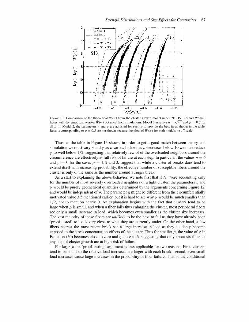
Turning to a comparison of this result with Monte Carlo simulations, Figure 13 compares
two versions of W(σ) in Equation (73) against W (σ ) from the Monte Carlo simulations, for
ρ = 1, 2, 3, 5 and 10. The dashed lines (Model 1) assume γ = 1/2 and η =√
4π ≈ 3.5,
as is the case in Equation (50) if we assume all fibers in the first ring around the cluster to be
equally at full risk of failure. The solid lines (Model 2) assume γ and η values corresponding
to the respective ρ values as shown in the table within the figure. The fit in the dashed line
case (Model 1), which is excellent for ρ = 20 (not shown) and quite good for ρ = 10, rapidly
deteriorates for ρ ≤ 5. However, except for ρ = 1, the agreement is excellent (Model 2) when
γ and η are adjusted as shown in the table within the figure.
Regarding the influence of η and γ in achieving a good fit for W(σ), we first note that
increasing η while keeping γ fixed corresponds to proportionately more fibers being at risk of
failure at the edge of a cluster of given size. Thus, increasing η approximately corresponds
to shifting the model lines upward in Figure 13. On the other hand, increasing γ with η
fixed results in increasing the number of cluster neighbors at risk of failure as the cluster
grows, but as a higher power of cluster size. Thus, a larger γ signifies greater sensitivity of
failure probability to increasing size. Therefore, the slope of the model W(σ) line in Figure 13
decreases when γ is increased. To achieve the fits shown in the figure there is actually very
little leeway in the tabulated values shown therein, as the positions of the theoretical lines are
very sensitive to the choices of γ and η. (For example, changing η from 6 to 5 ruins the fit.)
Note also that while many approximations were made in deriving W(σ) in Equation (73),
using the root equation, Equation (49), with Nr defined by Equation (50) does not change
these observations.
Strength Distributions and Size Effects for Composites 67
Figure 13. Comparison of the theoretical W(σ) from the cluster growth model under 2D HVLLS and Weibull
fibers with the empirical version W (σ ) obtained from simulations. Model 1 assumes η =√
4π and γ = 0.5 for
all ρ. In Model 2, the parameters η and γ are adjusted for each ρ to provide the best fit as shown in the table.
Results corresponding to ρ = 0.5 are not shown because the plots of W(σ) for both models lie off scale.
Thus, as the table in Figure 13 shows, in order to get a good match between theory and
simulation we must vary η and γ as ρ varies. Indeed, as ρ decreases below 10 we must reduce
γ to well below 1/2, suggesting that relatively few of of the overloaded neighbors around the
circumference are effectively at full risk of failure at each step. In particular, the values η = 6
and γ = 0 for the cases ρ = 1, 2 and 3, suggest that while a cluster of breaks does tend to
extend itself with increasing probability, the effective number of susceptible fibers around the
cluster is only 6, the same as the number around a single break.
As a start to explaining the above behavior, we note first that if Nr were accounting only
for the number of most severely overloaded neighbors of a tight cluster, the parameters η and
γ would be purely geometrical quantities determined by the arguments concerning Figure 12,
and would be independent of ρ. The parameter η might be different from the circumferentially
motivated value 3.5 mentioned earlier, but it is hard to see why γ would be much smaller than
1/2, not to mention nearly 0. An explanation begins with the fact that clusters tend to be
large when ρ is small, and when a fiber fails thus enlarging the cluster, most peripheral fibers
see only a small increase in load, which becomes even smaller as the cluster size increases.
The vast majority of these fibers are unlikely to be the next to fail as they have already been
‘proof-tested’ to loads very close to what they are currently under. On the other hand, a few
fibers nearest the most recent break see a large increase in load as they suddenly become
exposed to the stress concentration effects of the cluster. Thus for smaller ρ, the value of γ in
Equation (50) becomes close to zero and η close to 6, suggesting that only about six fibers at
any step of cluster growth are at high risk of failure.
For large ρ the ‘proof-testing’ argument is less applicable for two reasons: First, clusters
tend to be small so the relative load increases are larger with each break; second, even small
load increases cause large increases in the probability of fiber failure. That is, the conditional
68 S. Mahesh et al.
probability of fiber failure at load Krσ conditioned on its survival up to load Kr−1σ , that is,
(F (Krσ )−F(Kr−1σ ))/(1−F(Kr−1σ )), is well approximated by F(Krσ ) for small σ , when
ρ is large. These issues will be pursued further in Section 6.
The parameter β1 = (ρ + 4γ )/4 plays a role in the behavior of W(σ) through ?2(σ ) of
Equation (74), as ρ and γ diminish. Curiously, when γ = 0 we have β1 = ρ/4 suggesting
that the value ρ = 4 has special significance. We find that ?2(σ ) starts to increase rapidly
when ρ diminishes below 4 reflecting an increased cluster stalling probability. This has the
effect of decreasing W(σ), and thus, the probability of failure, though the effect is not strong
enough to explain the behavior of the simulations for small ρ in Figure 13, and especially
the sudden strength increase for ρ = 1/2 in Figure 13. The weakness of the fit for ρ = 1 is
consistent with the earlier observation in Figure 9, that once ρ decreases below about 2 the
δ-bundle failure distribution develops strong Gaussian character as seen under ELS, which is
truly a dispersed failure mode. This is also pursued in Section 6.
Equation (73) for W(σ) is very similar in form to that calculated by Wu and Leath (2000b)
for failure in a fuse network under variants of the local load sharing rule. Despite the differ-
ences in the precise nature of the load sharing rule, the exponential factor in Equation (73)
is identical to theirs to highest order. That is, Wu and Leath’s expression also has the fac-
tor exp(−?2(σ )(aσδ/σ )ρ/β1) if β1 is calculated using γ = 0.5. Their pre-exponential fac-
tors however are more sensitive to the nature of the load sharing and differ from those in
Equation (73).
4.4. SIZE EFFECT FOR CRITICAL CLUSTER AND COMPOSITE STRENGTH UNDER HVLLS
We now derive formulas for the variation of the critical cluster size k∗ with the size n of δ-
bundles under 2D HVLLS and at failure probability level p = 1 − 1/e. We then derive the
dependence of the characteristic δ-bundle strength σ ∗c on n. Converting this result to apply to
the full composite only requires replacing n by mn.
The first step is to set Wk = 1/n or, using Equation (61), we have
C(√
k + b)ϕ
exp
{
β1
(√k + b − β2
2β1
)2}
= nC. (75)
For moderate k∗, we note that√k∗ + b is close to β2/2β1, which makes the exponential
function in Equation (75) amenable to a power series expansion. Asymptotic inversion leads
to
log(√
k∗ + b)
= log(nC)+ log(ω1)
ϕ, (76)
where the correction term log(ω1) grows slowly with log(nC) following
log(ω1) =− β2
2
4β1
[
log(nC)
ϕ− log
(
β2
2β1
)]2
1 + β22
4β1ϕ
[
log(nC)
ϕ− log
(
β2
2β1
)]. (77)
The correction term ω1, while small, can have a major effect on the resulting k∗. The above
formula for k∗ works for a wide range of n (e.g., n < 109). However, for larger n, an expansion
arises of the form
Strength Distributions and Size Effects for Composites 69
√k∗ + b =
(√
log(nC)
β1
+ β2
2β1
)
(1 − ω2), (78)
where the correction term ω2 is
ω2 =ϕ log
(√
log(nC)
β1
+ β2
2β1
)
ϕ + 2 log(nC)+ β2
β1
√
log(nC)
β1
. (79)
For astronomical n such as n > 1025 we have
√k∗ + b =
√
log(nC)
β1
. (80)
Substituting for k∗ in terms of σ ∗ we estimate the size effect for the stress when the critical
cluster forms. From Equations (65) and (76) we get
σ ∗ ≈ aσδ
(
(nCω1)1/ϕ − bγ
β1
)−2β1/ρ
. (81)
For extremely large n, Equations (65) and (78) lead to
σ ∗ ≈ aσδ
((√
log(nC)
β1
+ β2
2β1
)
(1 − ω2)−bγ
β1
)−2β1/ρ
. (82)
Finally, as n → ∞, this behaves as
σ ∗ = aσδ
(
β1
log(nC)
)β1/ρ
. (83)
To obtain the characteristic stress for composite failure, σ ∗c , we must account for .1(σ ) and
.2(σ ) leading to complex expressions. We estimate the main effect by noting that ?2(σ ) → B
as σ → 0 where
B = 1 + 1
2β1(β1 + 1)+ 1
β21
�
(
1
β1
, 1
)
. (84)
Thus for large n we may obtain σ ∗c from σ ∗ upon replacing log(nC)/β1 by log(nC)/(Bβ1) in
Equations(82) and (83). For smaller n, of the order used in our simulations, and larger values
of ρ we can still use Equation (81) for σ ∗c . For smaller ρ, say ρ ≤ 5 where B differs apprecia-
bly from one, Equations (82) and (83) may be applied but are likely to be very conservative
as Bβ1 is a poor reflection of the full effect of ?2(σ ) in Equation (73).
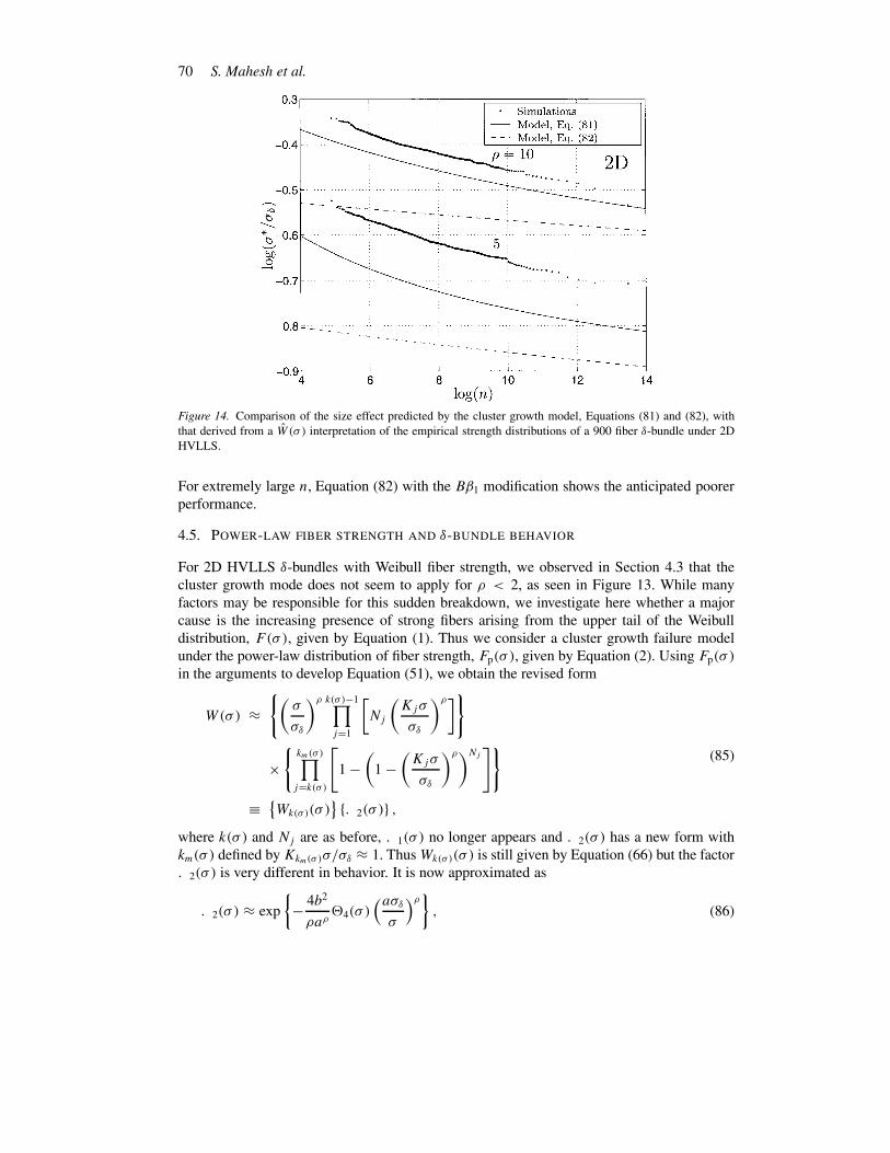
Figure 14 shows a plot of σ ∗ given by Equation (81) against the size effect predicted using
simulations from the δ-bundles of size n = 900 as though they posses weakest link character in
terms of W(σ ), as is supported by Figure 13. The size range covered is 100 < n < 1 000 000,
which is the relevant range for Equation (81). Clearly the formula works reasonably well for
ρ = 10 and has the right shape for ρ = 5, but breaks down for smaller ρ, mainly because
of the above mentioned lack of treatment of the cluster stalling probability in the derivation.
70 S. Mahesh et al.
Figure 14. Comparison of the size effect predicted by the cluster growth model, Equations (81) and (82), with
that derived from a W (σ ) interpretation of the empirical strength distributions of a 900 fiber δ-bundle under 2D
HVLLS.
For extremely large n, Equation (82) with the Bβ1 modification shows the anticipated poorer
performance.
4.5. POWER-LAW FIBER STRENGTH AND δ-BUNDLE BEHAVIOR
For 2D HVLLS δ-bundles with Weibull fiber strength, we observed in Section 4.3 that the
cluster growth mode does not seem to apply for ρ < 2, as seen in Figure 13. While many
factors may be responsible for this sudden breakdown, we investigate here whether a major
cause is the increasing presence of strong fibers arising from the upper tail of the Weibull
distribution, F(σ ), given by Equation (1). Thus we consider a cluster growth failure model
under the power-law distribution of fiber strength, Fp(σ ), given by Equation (2). Using Fp(σ )
in the arguments to develop Equation (51), we obtain the revised form
W(σ) ≈{
(
σ
σδ
)ρ k(σ )−1∏
j=1
[
Nj
(
Kjσ
σδ
)ρ]}
×{
km(σ )∏
j=k(σ )
[
1 −(
1 −(
Kjσ
σδ
)ρ)Nj]}
≡{
Wk(σ )(σ )}
{.2(σ )} ,
(85)
where k(σ ) and Nj are as before, .1(σ ) no longer appears and .2(σ ) has a new form with
km(σ ) defined by Kkm(σ )σ/σδ ≈ 1. Thus Wk(σ )(σ ) is still given by Equation (66) but the factor
.2(σ ) is very different in behavior. It is now approximated as
.2(σ ) ≈ exp
{
− 4b2
ρaρ@4(σ )
(aσδ
σ
)ρ}
, (86)
Strength Distributions and Size Effects for Composites 71
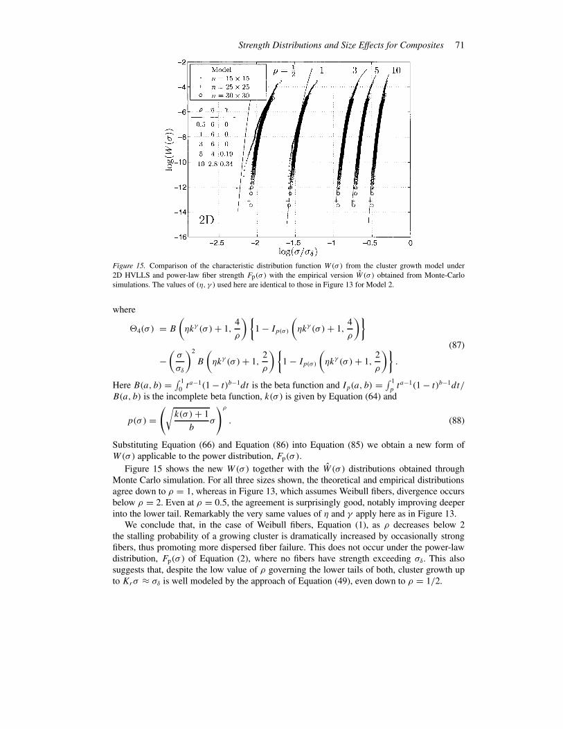
Figure 15. Comparison of the characteristic distribution function W(σ) from the cluster growth model under
2D HVLLS and power-law fiber strength Fp(σ ) with the empirical version W (σ ) obtained from Monte-Carlo
simulations. The values of (η, γ ) used here are identical to those in Figure 13 for Model 2.
where
@4(σ ) = B
(
ηkγ (σ )+ 1,4
ρ
){
1 − Ip(σ)
(
ηkγ (σ )+ 1,4
ρ
)}
−(
σ
σδ
)2
B
(
ηkγ (σ )+ 1,2
ρ
){
1 − Ip(σ)
(
ηkγ (σ )+ 1,2
ρ
)}
.
(87)
Here B(a, b) =∫ 1
0ta−1(1 − t)b−1dt is the beta function and Ip(a, b) =
∫ 1
pta−1(1 − t)b−1dt/
B(a, b) is the incomplete beta function, k(σ ) is given by Equation (64) and
p(σ ) =(
√
k(σ )+ 1
bσ
)ρ
. (88)
Substituting Equation (66) and Equation (86) into Equation (85) we obtain a new form of
W(σ) applicable to the power distribution, Fp(σ ).
Figure 15 shows the new W(σ) together with the W(σ ) distributions obtained through
Monte Carlo simulation. For all three sizes shown, the theoretical and empirical distributions
agree down to ρ = 1, whereas in Figure 13, which assumes Weibull fibers, divergence occurs
below ρ = 2. Even at ρ = 0.5, the agreement is surprisingly good, notably improving deeper
into the lower tail. Remarkably the very same values of η and γ apply here as in Figure 13.
We conclude that, in the case of Weibull fibers, Equation (1), as ρ decreases below 2
the stalling probability of a growing cluster is dramatically increased by occasionally strong
fibers, thus promoting more dispersed fiber failure. This does not occur under the power-law
distribution, Fp(σ ) of Equation (2), where no fibers have strength exceeding σδ. This also
suggests that, despite the low value of ρ governing the lower tails of both, cluster growth up
to Krσ ≈ σδ is well modeled by the approach of Equation (49), even down to ρ = 1/2.
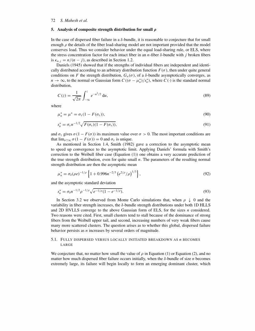
72 S. Mahesh et al.
5. Analysis of composite strength distribution for small ρ
In the case of dispersed fiber failure in a δ-bundle, it is reasonable to conjecture that for small
enough ρ the details of the fiber load-sharing model are not important provided that the model
conserves load. Thus we consider behavior under the equal load-sharing rule, or ELS, where
the stress concentration factor for each intact fiber in an n-fiber δ-bundle with j broken fibers
is κn,j = n/(n− j), as described in Section 1.2.
Daniels (1945) showed that if the strengths of individual fibers are independent and identi-
cally distributed according to an arbitrary distribution function F(σ ), then under quite general
conditions on F the strength distribution, Gn(σ ), of a δ-bundle asymptotically converges, as
n → ∞, to the normal or Gaussian form C((σ − µ∗n)/s
∗n), where C(·) is the standard normal
distribution,
C(z) = 1√2π
∫ z
−∞e−u2/2 du, (89)
where
µ∗n = µ∗ = στ (1 − F(στ )), (90)
s∗n = στn−1/2
√
F(στ )(1 − F(στ )), (91)
and στ gives σ (1−F(σ )) its maximum value over σ > 0. The most important conditions are
that limσ↑∞ σ (1 − F(σ )) = 0 and στ is unique.
As mentioned in Section 1.4, Smith (1982) gave a correction to the asymptotic mean
to speed up convergence to the asymptotic limit. Applying Daniels’ formula with Smith’s
correction to the Weibull fiber case (Equation (1)) one obtains a very accurate prediction of
the true strength distribution, even for quite small n. The parameters of the resulting normal
strength distribution are then the asymptotic mean
µ∗n = σδ(ρe)
−1/ρ{
1 + 0.996n−2/3(
e2/ρ/ρ)1/3
}
, (92)
and the asymptotic standard deviation
s∗n = σδn−1/2ρ−1/ρ
√
e−1/ρ(1 − e−1/ρ). (93)
In Section 3.2 we observed from Monte Carlo simulations that, when ρ ↓ 0 and the
variability in fiber strength increases, the δ-bundle strength distributions under both 1D HLLS
and 2D HVLLS converge to the above Gaussian form of ELS, for the sizes n considered.
Two reasons were cited. First, small clusters tend to stall because of the dominance of strong
fibers from the Weibull upper tail, and second, increasing numbers of very weak fibers cause
many more scattered clusters. The question arises as to whether this global, dispersed failure
behavior persists as n increases by several orders of magnitude.
5.1. FULLY DISPERSED VERSUS LOCALLY INITIATED BREAKDOWN AS n BECOMES
LARGE
We conjecture that, no matter how small the value of ρ in Equation (1) or Equation (2), and no
matter how much dispersed fiber failure occurs initially, when the δ-bundle of size n becomes
extremely large, its failure will begin locally to form an emerging dominant cluster, which
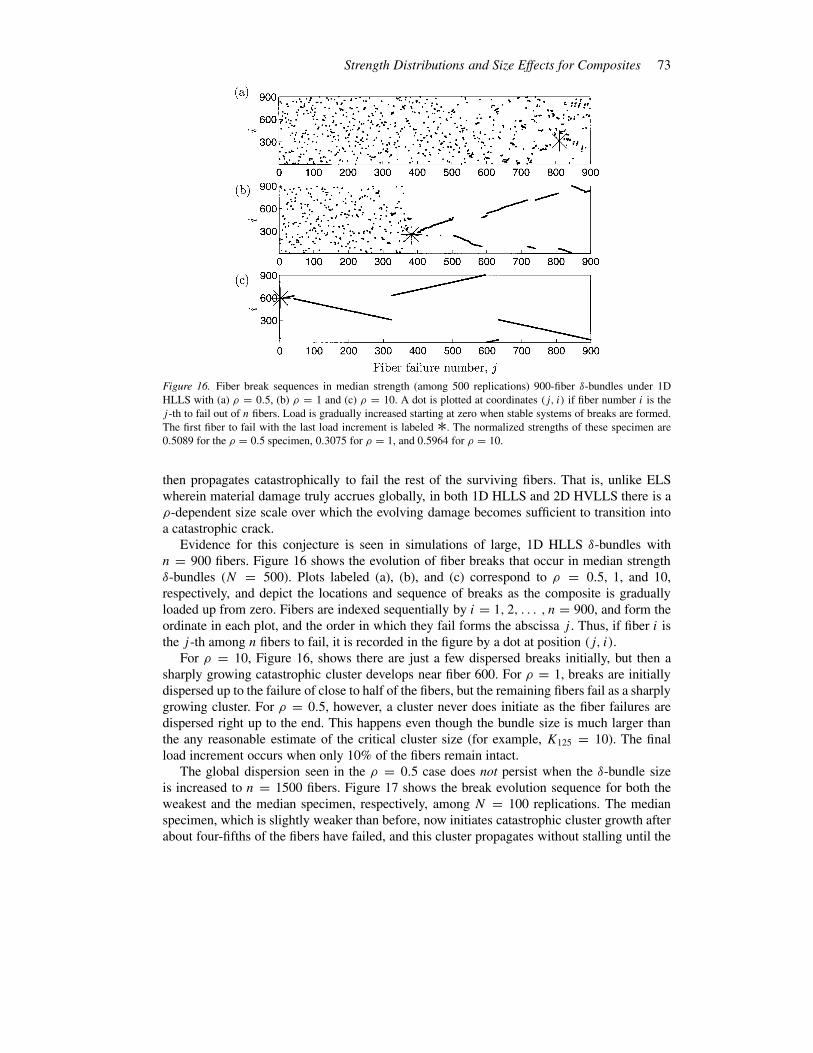
Strength Distributions and Size Effects for Composites 73
Figure 16. Fiber break sequences in median strength (among 500 replications) 900-fiber δ-bundles under 1D
HLLS with (a) ρ = 0.5, (b) ρ = 1 and (c) ρ = 10. A dot is plotted at coordinates (j, i) if fiber number i is the
j -th to fail out of n fibers. Load is gradually increased starting at zero when stable systems of breaks are formed.
The first fiber to fail with the last load increment is labeled ∗. The normalized strengths of these specimen are
0.5089 for the ρ = 0.5 specimen, 0.3075 for ρ = 1, and 0.5964 for ρ = 10.
then propagates catastrophically to fail the rest of the surviving fibers. That is, unlike ELS
wherein material damage truly accrues globally, in both 1D HLLS and 2D HVLLS there is a
ρ-dependent size scale over which the evolving damage becomes sufficient to transition into
a catastrophic crack.
Evidence for this conjecture is seen in simulations of large, 1D HLLS δ-bundles with
n = 900 fibers. Figure 16 shows the evolution of fiber breaks that occur in median strength
δ-bundles (N = 500). Plots labeled (a), (b), and (c) correspond to ρ = 0.5, 1, and 10,
respectively, and depict the locations and sequence of breaks as the composite is gradually
loaded up from zero. Fibers are indexed sequentially by i = 1, 2, . . . , n = 900, and form the
ordinate in each plot, and the order in which they fail forms the abscissa j . Thus, if fiber i is
the j -th among n fibers to fail, it is recorded in the figure by a dot at position (j, i).
For ρ = 10, Figure 16, shows there are just a few dispersed breaks initially, but then a
sharply growing catastrophic cluster develops near fiber 600. For ρ = 1, breaks are initially
dispersed up to the failure of close to half of the fibers, but the remaining fibers fail as a sharply
growing cluster. For ρ = 0.5, however, a cluster never does initiate as the fiber failures are
dispersed right up to the end. This happens even though the bundle size is much larger than
the any reasonable estimate of the critical cluster size (for example, K125 = 10). The final
load increment occurs when only 10% of the fibers remain intact.
The global dispersion seen in the ρ = 0.5 case does not persist when the δ-bundle size
is increased to n = 1500 fibers. Figure 17 shows the break evolution sequence for both the
weakest and the median specimen, respectively, among N = 100 replications. The median
specimen, which is slightly weaker than before, now initiates catastrophic cluster growth after
about four-fifths of the fibers have failed, and this cluster propagates without stalling until the
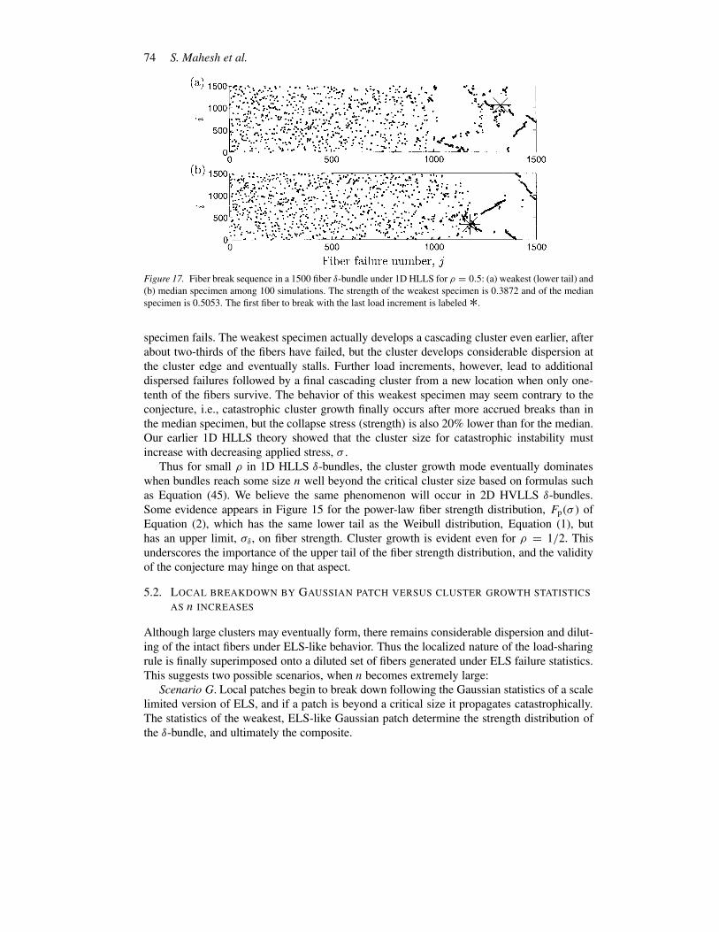
74 S. Mahesh et al.
Figure 17. Fiber break sequence in a 1500 fiber δ-bundle under 1D HLLS for ρ = 0.5: (a) weakest (lower tail) and
(b) median specimen among 100 simulations. The strength of the weakest specimen is 0.3872 and of the median
specimen is 0.5053. The first fiber to break with the last load increment is labeled ∗.
specimen fails. The weakest specimen actually develops a cascading cluster even earlier, after
about two-thirds of the fibers have failed, but the cluster develops considerable dispersion at
the cluster edge and eventually stalls. Further load increments, however, lead to additional
dispersed failures followed by a final cascading cluster from a new location when only one-
tenth of the fibers survive. The behavior of this weakest specimen may seem contrary to the
conjecture, i.e., catastrophic cluster growth finally occurs after more accrued breaks than in
the median specimen, but the collapse stress (strength) is also 20% lower than for the median.
Our earlier 1D HLLS theory showed that the cluster size for catastrophic instability must
increase with decreasing applied stress, σ .
Thus for small ρ in 1D HLLS δ-bundles, the cluster growth mode eventually dominates
when bundles reach some size n well beyond the critical cluster size based on formulas such
as Equation (45). We believe the same phenomenon will occur in 2D HVLLS δ-bundles.
Some evidence appears in Figure 15 for the power-law fiber strength distribution, Fp(σ ) of
Equation (2), which has the same lower tail as the Weibull distribution, Equation (1), but
has an upper limit, σδ, on fiber strength. Cluster growth is evident even for ρ = 1/2. This
underscores the importance of the upper tail of the fiber strength distribution, and the validity
of the conjecture may hinge on that aspect.
5.2. LOCAL BREAKDOWN BY GAUSSIAN PATCH VERSUS CLUSTER GROWTH STATISTICS
AS n INCREASES
Although large clusters may eventually form, there remains considerable dispersion and dilut-
ing of the intact fibers under ELS-like behavior. Thus the localized nature of the load-sharing
rule is finally superimposed onto a diluted set of fibers generated under ELS failure statistics.
This suggests two possible scenarios, when n becomes extremely large:
Scenario G. Local patches begin to break down following the Gaussian statistics of a scale
limited version of ELS, and if a patch is beyond a critical size it propagates catastrophically.
The statistics of the weakest, ELS-like Gaussian patch determine the strength distribution of
the δ-bundle, and ultimately the composite.
Strength Distributions and Size Effects for Composites 75
Scenario W. Broad dilution of the number of surviving fibers occurs due to ELS-like behav-
ior, but local cluster growth eventually develops under a revised local load sharing mechanism
on the randomly diluted set of survivors. The result would be cluster-dominated failure under
a characteristic distribution function, W(σ), which is a revised version of that obtained earlier
for larger ρ.
A model consistent with Scenario G is that failure initiates following an ELS-like failure
mechanism in a patch of n fibers smaller than n when sufficiently large. Such a model has
been studied by Ibnabdeljalil and Curtin (1997), Curtin and Takeda (1998) and Curtin (1998).
The patch strength has Gaussian character, and δ-bundle failure corresponds to the failure of
the weakest of the m = n/n patches. That is
Gn(σ ) = 1 − {1 −C[(σ − µ∗n)/s
∗n]}m, (94)
where C(·) is the standard normal distribution, and µ∗n
and σ ∗n
are as defined in Equations (92)
and (93). For small σ , we may replace C(·) with
C(z) = 1√2π |z|
exp(−z2/2), (95)
which is the asymptotic form of the lower tail of C(z). Likewise, Hm,n(σ ) for the composite
is simply the above result with m replaced by mm. The parameters of the Gaussian patch are
given by the Smith corrected, Daniels formula Equation (92) and (93). Use of this result in
other composite settings is found in Phoenix et al. (1997).
In Figure 18, for the cases ρ = 1/2, 1, 2, 3 and 5 we have plotted the strength distribution of
the smallest sized δ-bundle (n1×n1) to which weak-link scaled distributions for larger bundles
collapse. This minimum δ-bundle size approximately corresponds to the critical cluster size
defined previously. We also show the strength distributions for larger bundles of size (n2 ×n2)
or (n3×n3) scaled to the size (n1×n1). As ρ decreases, the weak-linked distributions become
increasingly Gaussian (indicated by the straightness of the strength distribution on normal
coordinates) and are better approximated by the ELS asymptotic distribution, though a mean
shift exists for ρ ≥ 1, indicative of local load enhancement effects. Similar observations,
including the mean shift, were noted by Curtin (1998), using a comparable model but for a
square fiber array with ρ = 3, 5, and 10.
In the case ρ = 0.5, however, despite the excellent agreement of the 900-fiber, δ-bundle
strength distribution weak-link scaled to that for 625 fibers, this weak-link scaling does not
work for a 2500-fiber, δ-bundle scaled to 625 fibers (of which limited results were generated
but are not shown). This suggests that the smallest ultimate catastrophic failure event of the
bundle occurs over more than 625 fibers, or perhaps even 900 fibers. The same may also be
true in the ρ = 1 case. However, for ρ ≥ 2, the maximum simulation cell size of n = 30× 30
seems to be adequate to contain the catastrophic failure event.
For 2D HVLLS, a comparison of Figures 18 and 13 suggests that there is a small range
for ρ, say between 1 and 2, where models for Scenario G and Scenario W both match the
simulations fairly well. In Scenario G, however, the ELS form for the mean, Equation (92),
overestimates the true simulated mean for ρ > 1, whereas the model for Scenario W un-
derestimates the mean for ρ < 2. On the other hand, a comparison to results in Figures 15
and 10 reveals the crucial role of the upper tail of the Weibull fiber strength distribution,
F(σ ); if fibers with strength above σδ are removed δ-bundle strength drops dramatically as
Scenario W behavior suddenly dominates. In the cluster growth model of Section 4, the upper
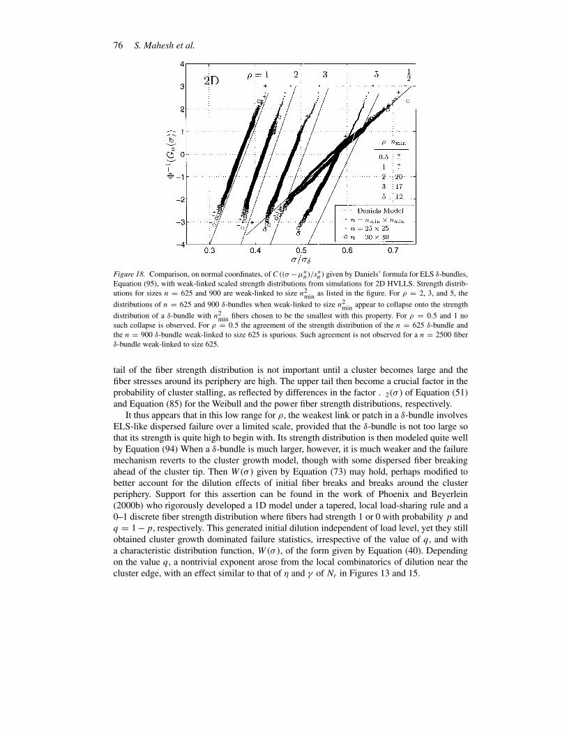
76 S. Mahesh et al.
Figure 18. Comparison, on normal coordinates, of C((σ −µ∗n)/s
∗n) given by Daniels’ formula for ELS δ-bundles,
Equation (95), with weak-linked scaled strength distributions from simulations for 2D HVLLS. Strength distrib-
utions for sizes n = 625 and 900 are weak-linked to size n2min
as listed in the figure. For ρ = 2, 3, and 5, the
distributions of n = 625 and 900 δ-bundles when weak-linked to size n2min
appear to collapse onto the strength
distribution of a δ-bundle with n2min
fibers chosen to be the smallest with this property. For ρ = 0.5 and 1 no
such collapse is observed. For ρ = 0.5 the agreement of the strength distribution of the n = 625 δ-bundle and
the n = 900 δ-bundle weak-linked to size 625 is spurious. Such agreement is not observed for a n = 2500 fiber
δ-bundle weak-linked to size 625.
tail of the fiber strength distribution is not important until a cluster becomes large and the
fiber stresses around its periphery are high. The upper tail then become a crucial factor in the
probability of cluster stalling, as reflected by differences in the factor .2(σ ) of Equation (51)
and Equation (85) for the Weibull and the power fiber strength distributions, respectively.
It thus appears that in this low range for ρ, the weakest link or patch in a δ-bundle involves
ELS-like dispersed failure over a limited scale, provided that the δ-bundle is not too large so
that its strength is quite high to begin with. Its strength distribution is then modeled quite well
by Equation (94) When a δ-bundle is much larger, however, it is much weaker and the failure
mechanism reverts to the cluster growth model, though with some dispersed fiber breaking
ahead of the cluster tip. Then W(σ) given by Equation (73) may hold, perhaps modified to
better account for the dilution effects of initial fiber breaks and breaks around the cluster
periphery. Support for this assertion can be found in the work of Phoenix and Beyerlein
(2000b) who rigorously developed a 1D model under a tapered, local load-sharing rule and a
0–1 discrete fiber strength distribution where fibers had strength 1 or 0 with probability p and
q = 1−p, respectively. This generated initial dilution independent of load level, yet they still
obtained cluster growth dominated failure statistics, irrespective of the value of q, and with
a characteristic distribution function, W(σ), of the form given by Equation (40). Depending
on the value q, a nontrivial exponent arose from the local combinatorics of dilution near the
cluster edge, with an effect similar to that of η and γ of Nr in Figures 13 and 15.
Strength Distributions and Size Effects for Composites 77
None of the above issues can be resolved satisfactorily until computational power increases
to the point where much larger bundles can be treated. Presently we cannot simulate δ-bundles
much beyond n = 1500, and under 2D HVLLS and ρ = 0.5 the cluster size required for
catastrophic instability is probably much greater.
6. Analysis of effect of ρ on the statistical failure mode
We have seen that the failure of moderately-sized δ-bundles, for both 1D HLLS and 2D
HVLLS, tends to show a transition from a break cluster growth mode to a dispersed failure
mode somewhere in the neighborhood of ρ = 1 to 2. We also found that Nr , the effective
number of ‘high risk’ fibers neighboring an r-cluster, appears to depend on ρ, and is not the
number of fibers around the cluster circumference. We investigate these two issues further in
this section.
6.1. EFFECT OF ρ ON CLUSTER GROWTH AT ITS EDGE
To investigate the effect of decreasing ρ on cluster growth, we consider a stable r-cluster and
add one break to form an (r + 1)-cluster. We let E(r, n′) be the mean number of fibers among
its n′ nearest intact neighbors that will fail due to the increased load from this break, assuming
all fibers have survived the previous load, i.e., have been ‘proof-tested’. We let the applied
fiber stress σ be small enough that the fiber failure probability F(Krσ ) from Equation (1) is
well approximated by F(Krσ ) ≈ (Krσ/σδ)ρ . Then,
E(r, n′) ≈ n′(Kρ
r+1 −Kρr ) (σ/σδ)
ρ . (96)
When ρ is large the prefactor n′(Kρ
r+1 − Kρr ) is an increasing function of ρ since Kr+1 >
Kr > 1. Furthermore, Kρ
r+1 increasingly dominates Kρr as ρ increases, especially when r is
fairly small. Thus
n′(Kρ
r+1 −Kρr )
n′Kρ
r+1
→ 1, as ρ → ∞. (97)
Thus, when ρ is large so that the cluster size is fairly small, previous survival of a fiber
under stress Krσ has little effect on the likelihood of its failure under Kr+1σ . All fibers around
the periphery of a cluster are equally at risk of failure, behaving as though they are virgin
fibers.
To see what may happen for small ρ in the case of 2D HVLLS, we specialize Equation (96)
to a large circular r-cluster in a δ-bundle. Then n′ ≈ 2√π(r + 1), and using Equation (16),
we get
E(r, n′) ≈ 2√
π(r + 1)
(
1 + 2√r + 1
π3/2
)ρ2
−(
1 + 2√r
π3/2
)
ρ2
(
σ
σδ
)ρ
,
≈ Cρrρ4− 1
2
(
σ
σδ
)ρ
, for large r,
(98)
where Cρ is some constant. Significantly, the power on r is ρ/4−1/2, and furthermore, ρ = 2
is a transition value below which the number of new breaks actually decreases as r increases,
thus increasing the tendency of such a cluster to stall.
78 S. Mahesh et al.
If however, we consider the case where all fibers are virgin, the second term in the brackets
can be ignored, and the power on r becomes ρ/4+1/2, i.e., larger by 1. An intermediate case
is where all fibers have been proof-tested only up to a cluster diameter, D−1 (i.e., without the
outer ring of failed fibers). In that case, r = πD2/4, and the power on r turns out to be ρ/4.
Note that in our model the power on r is β1 = ρ/4 + γ , so this latter situation corresponds to
γ = 0 and the former to γ = 1/2. Neither case shows a transitional ρ.
The calculation in Equation (98), however does not account for the fact that the occurrence
of a single break at a cluster edge will always expose a few of its immediate neighbors (say
N0 ≈ 3) to a much larger jump in stress of order (1/2)Krσ/σδ to Kr+1σ/σδ. The total
probability of failure is approximately N0(Kr+1σ/σδ)ρ , which also asymptotically depends
on r with exponent ρ/4. This also does not show the above transitional ρ, and in fact, has
scaling like the case above where proof-testing is only to a cluster diameter, D, smaller by
one. Depending on ρ, the true situation in large cluster growth is a combination of the present
case and a mixture of the two proof-test cases above, with a power perhaps a little less than
ρ/4. Thus, as ρ decreases to 2, Nr becomes independent of r and takes a constant value, which
is at least N0 ≈ 3 and apparently is 6 based on the simulations. Next we consider why this
doubly larger value emerges.
6.2. EFFECT OF ρ ON DISPERSED BREAKS NEAR CLUSTER EDGE
An important aspect to consider, as ρ decreases, is the location of new breaks due to an r-
cluster in a δ-bundle. Figure 19 shows a simulation of the fiber failures that immediately
occur due to the introduction of a penny-shaped cluster of r = 239 breaks under the numerical
version 2D HVLLS. In each of the four cases, the fiber strengths were derived from the same
set of uniformly distributed random numbers Ui , so the Weibull strength of the i-th fiber
in each case is (− log(Ui))1/ρ. In each case the applied stress, σ , was chosen so that the
probability of failure of a fiber adjacent to the cluster edge was about 1/2, i.e., (K239σ/σδ)ρ ≈
0.69, where K239 = 2.56 from Equation (16). These breaks would typically cause secondary
breaks without a change in applied load, but such breaks are not shown. Observe that for the
same approximate number of fiber failures in the ring around the cluster, an increasing number
occur away from the cluster, as ρ is decreased. Many breaks appearing for ρ = 1/2, 1 and 3
would have occurred anyway under stress σ , but nevertheless, dispersive effects at the edge
begin to appear.
To understand these dispersive effects, we evaluate the probability of failure of a fiber
at distance s away from the cluster edge. Its probability of failure is (Kr,sσ/σδ)ρ or, using
Equation (17),
Pr{fiber failure at distance s} =(
1
1 + π(s − 1)
)ρ/2 (Krσ
σδ
)ρ
. (99)
This result holds approximately for 1 ≤ s ≤ 1+ εD/2 where ε ≈ 1/3 and D = 2√r/π is the
cluster diameter. This is roughly the range of influence of the cluster ‘tip’ (analogous to the
K-field in linear elastic fracture mechanics). Clearly the first factor in Equation (99) increases
with decreasing ρ, and leads to a relative increase in number of failures away from the cluster
edge. Beyond this range the stress is close to the far field value, σ . In the present case r = 239,
D ≈ 18, and the range covers just two fibers. Nevertheless one can see increasing breaks in
the sub-adjacent rings, as ρ decreases.
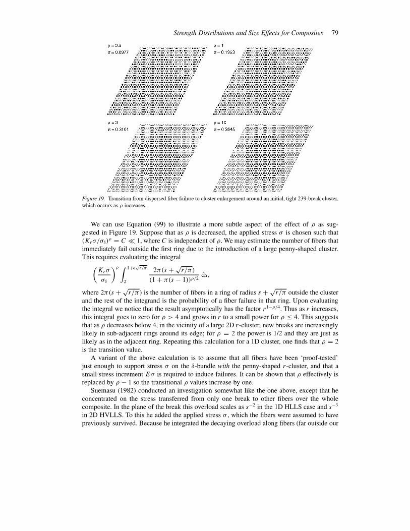
Strength Distributions and Size Effects for Composites 79
Figure 19. Transition from dispersed fiber failure to cluster enlargement around an initial, tight 239-break cluster,
which occurs as ρ increases.
We can use Equation (99) to illustrate a more subtle aspect of the effect of ρ as sug-
gested in Figure 19. Suppose that as ρ is decreased, the applied stress σ is chosen such that
(Krσ/σδ)ρ = C � 1, where C is independent of ρ. We may estimate the number of fibers that
immediately fail outside the first ring due to the introduction of a large penny-shaped cluster.
This requires evaluating the integral
(
Krσ
σδ
)ρ ∫ 1+ε√r/π
2
2π(s +√r/π)
(1 + π(s − 1))ρ/2ds,
where 2π(s +√r/π) is the number of fibers in a ring of radius s +
√r/π outside the cluster
and the rest of the integrand is the probability of a fiber failure in that ring. Upon evaluating
the integral we notice that the result asymptotically has the factor r1−ρ/4. Thus as r increases,
this integral goes to zero for ρ > 4 and grows in r to a small power for ρ ≤ 4. This suggests
that as ρ decreases below 4, in the vicinity of a large 2D r-cluster, new breaks are increasingly
likely in sub-adjacent rings around its edge; for ρ = 2 the power is 1/2 and they are just as
likely as in the adjacent ring. Repeating this calculation for a 1D cluster, one finds that ρ = 2
is the transition value.
A variant of the above calculation is to assume that all fibers have been ‘proof-tested’
just enough to support stress σ on the δ-bundle with the penny-shaped r-cluster, and that a
small stress increment Eσ is required to induce failures. It can be shown that ρ effectively is
replaced by ρ − 1 so the transitional ρ values increase by one.
Suemasu (1982) conducted an investigation somewhat like the one above, except that he
concentrated on the stress transferred from only one break to other fibers over the whole
composite. In the plane of the break this overload scales as s−2 in the 1D HLLS case and s−3
in 2D HVLLS. To this he added the applied stress σ , which the fibers were assumed to have
previously survived. Because he integrated the decaying overload along fibers (far outside our
80 S. Mahesh et al.
δ-bundles), he concluded for all ρ > 0 that divergence occurs in the number of flaws broken
in all fibers over the whole composite. However, repeating his calculation over fibers within
a δ-bundle leads to convergence for all ρ > 0. Thus, little insight into the role of ρ is gained
without focusing on large clusters with 1/√s fiber stress decay at their edges.
These arguments indicate that during δ-bundle failure under increasing σ , the tendency
toward dispersed fiber failures versus cluster growth increases as ρ decreases, but the critical
values of ρ, from 2 to 4, seem too high to directly explain any apparent transitions seen in the
simulations, for ρ close to 1. Also, when ρ is small, the probability of finding very weak fibers
below strength σ is much more than when ρ is large, and thus many dispersed fiber breaks are
to be expected anyway. This aspect appears to be borne out by Figures 3 and 7, and Figure 19
as well as by inspection of many simulations.
At the same time, the number of fibers n in the δ-bundle plays a role as smaller composites
tend to be stronger, and thus, show a higher proportion of dispersed fiber breaks under the
applied stress σ . Also, clusters are smaller when they become unstable. In larger composites,
the cluster size required for instability is larger, mainly because the applied stress σ is smaller
(i.e., the composite is weaker) and a higher stress concentration at the cluster edge is needed
to fail fibers. Nevertheless, no matter how large the cluster is before instability, the tendency
when ρ is small is to form dispersed breaks at the cluster edge, eventually lowering the stress
concentration.
6.3. EXPLANATION FOR POWER-LAW FORM OF Nr AND DEPENDENCE ON ρ
Combining the two discussions above, we have the following implications with respect to
modeling cluster growth for various ρ: When ρ is large, say 20, clusters are inherently small
before instability and our method reflected in Equation (49) is valid with the effective Nr
being approximately the number of fibers around the cluster circumference. Although this
case is not shown in Figure 13 the corresponding values η = 3.5 and γ = 1/2 work very
well. As ρ decreases, however, clusters become larger, and the decreasing power on r seen
in Equation (98) has the same effect as reducing the proportion of circumferential neighbors
taken to be at full risk in the approximation, Equation (49). This is captured by the lower
power on r in Nr . As ρ decreases toward 2, however, Nr becomes independent of r, and
reflects the number of freshly exposed immediate neighbors of the new break plus an equal
number close by in neighboring rings, to total about 6. All this is seen in Figures 13 and 15. It
might seem that, in the above argument, the probability of failure of all fibers in an r-cluster
solely under the initial stress σ is being ignored, but this is approximately (σ/σδ)rρ , which
is negligible compared to W(σ). Thus we have the ‘proof-test’ argument for why Nr is well
modeled by the power form Equation (50). This power form may be an oversimplification, but
power behavior in r does arise in the above calculations.
The above issue did not arise in 1D HLLS, because there were always just two neighbors to
a cluster and load increments were always large by comparison. Nevertheless, a small effect
arises there too, as can be seen for the case of two adjacent beaks. From Equation (23) we
have W2(σ ) ≈ 2F(σ )F (K1σ ), but more precisely this should be 2F(σ )F (K1σ ) − F(σ )2.
The first approximation subtly double counts the probability of failure of the two fibers under
the applied stress σ alone, when F(K1σ ) � F(σ ) i.e., the proof-testing effect is ignored.
The effect expands to multiple-counting for larger numbers of breaks, but in 1D it has little
practical consequence even for ρ very small. In 2D HVLLS, however, the problem is far worse
Strength Distributions and Size Effects for Composites 81
and lies at the heart of why the approximation, Equation (49), breaks down for smaller ρ if Nr
is taken simply as the number of fibers around the circumference.
Finally, when ρ is small, critical clusters from simulations do not tend to be round and may
be very distorted, with some intact bridging fibers at their fringes, as seen in Curtin (1998).
Indeed they may be hard to visually identify as true clusters. This raises the question of why
a tight cluster growth model should work at all for small ρ. In their 1D model with 0–1 fibers,
Phoenix and Beyerlein (2000b) showed rigorously that cluster growth behavior dominates
with a well defined W(σ) even though the dominant clusters had a wide variety of geometries
with bridging fibers near their fringes and were embedded in bundles with extensive dilution
by initial breaks. This suggests that a model that highly idealizes the cluster geometry may
still yield an accurate approximation to the probability of δ-bundle failure, as our simulations
seem to confirm.
7. Conclusions and relations to other results
In Equations (40) and (73) we have the weakest-link, characteristic distribution function,
W(σ), for 1D and 2D δ-bundles under HLLS and HVLLS, respectively, and assuming Weibull
fibers, Equation (1). These bundles are links in the chain-of-bundles model for the failure
of large 2D and 3D unidirectional composites, respectively. For sufficiently large Weibull
modulus ρ, say ρ ≥ 2 in 3D composites and ρ ≥ 1 in 2D planar composites, the strength
distribution of a composite of length L = mδ and with n fibers is Hm,n(σ ) ≈ 1 − (1 −W(σ))mn. When ρ decreases below these values, however, the details of the load-sharing be-
come increasingly unimportant, and the δ-bundle strength distribution is not only increasingly
Gaussian up to quite large n but also converges to that for ELS whose analytical form was
given. For fixed ρ, however, this Gaussian nature persists only up to a δ-bundle size n of the
order of the critical cluster size, slightly increased perhaps to fully eliminate the likelihood of
stalling. Then the distribution function for δ-bundle strength appears to be that for a chain of n-
fiber Gaussian ‘patches’ in the δ-bundle, particularly under 2D HVLLS. Thus the composite
can be viewed as a weakest-link arrangement of mm such Gaussian patches. However, as
the number of fibers n increases by orders of magnitude, this Gaussian patch nature may
not persist. In 1D HLLS and in 2D HVLLS under power-law fiber strength, Equation (2),
Gaussian patch behavior seems absent in favor of a cluster growth mode.
Simpler versions of the form for W(σ), Equation (40), have been derived in related failure
models where elements have strength 0 or 1 with probability p and 1−p, respectively. See for
example Duxbury and Leath (1987), Harlow and Phoenix (1991) and Phoenix and Beyerlein
(2000b), where in the latter two works power prefactors were obtained in W(σ) as here. As
mentioned earlier, very recent work carried out by Wu and Leath (2000a, b) under similar
assumptions, has yielded distribution forms very similar to those here. Earlier versions are
also given in Phoenix and Beyerlein (2000a), but none have the more general power form of
Nr used here.
In the time dependent setting, with a breakdown rate that is a power-law in stress with
exponent, ρ, analogous versions of W(t) have been obtained both without a power prefactor
by Curtin and Scher (1997) and Curtin et al. (1997), and with a power factor by Newman and
Phoenix (2001). In these works a hard transition to Gaussian lifetime behavior was noted when
ρ decreased below a certain critical value. Under ILLS mentioned in Section 1.2, Newman
and Phoenix (2001) showed that this hard transition occurs at ρ = 1. In the case of local load
82 S. Mahesh et al.
sharing similar to 1D HLLS and 2D HVLLS here, Curtin and Scher (1991) gave a mean-field
scaling calculation for the size of the catastrophic cluster which showed a hard transition at
ρ = 2 in 2D and ρ = 4 in 3D. The time dependent case and the case here are not directly
analogous, however, as there is a drastic change in the probability of cluster stalling right at
the transition value of ρ, which does not occur in our .2(σ ). This is a consequence of the
‘memoryless property’ in the time-dependent model.
Fiber break clusters need not lie in a transverse plane but can wander out of plane since
new breaks can form next to old ones anywhere within length δ. However the tendency toward
alignment is fairly strong unless the variability in fiber strength along the fiber is large. It is
known that this variability is often much less than the variability across fibers, which is the
object of this study. Nevertheless, the idea of using a single length-scale, δ, for fiber load
transfer may be unrealistic when large break clusters develop before instability. Thus the
chain-of-bundles concept may be too restrictive in certain cases and the load-sharing model
may require revision beyond using the fiber load values obtained along a single break plane.
To account for some of these features, simulation results have been generated by Landis
et al. (2000) for a true 3D model using a modified, square array version of HVLLS with
eight matrix shear couplings rather than four. Their results were successfully modeled by
Phoenix and Beyerlein (2000a) using the Gaussian-link approach, as described at the end of
the last section, but generalized to elastic global load-sharing. Using the W(σ) cluster growth
approach here Phoenix and Beyerlein (2000a) were only able to model quite well their results
for ρ = 20 but not ρ = 10 and 5 where misfits similar to those appearing in Figure 13
occurred. As here, using Equation (50) for Nr and adjusting γ and η should provide a good
match but only for ρ down to about 5 as the dispersive effects of out of plane breaks become
important.
In a true 3D model, failure by cluster growth will involve cluster extension by breakage of
fibers ahead of it as in the planar case discussed in this work; however these breaks need not
in general all lie in a common plane perpendicular to the fiber direction. Staggering of fiber
breaks greatly reduces stress concentrations ahead of the cluster thereby inducing dominance
of the global failure mechanism for larger ρ than in the planar case. Modeling of cluster
growth in a true 3D model is discussed in depth in Chapter 3 of Mahesh (2002) in the time
dependent setting. It is found that the only major modification necessary to the present model
is to capture the reduction of the stress concentration ahead of a cluster of staggered breaks.
This is done by taking the stress concentration to be of the form
Kr =√
πr
4ψ + 1 (100)
for 2D arrays and
Kr =
√
2√r
π3/2ψ + 1 (101)
in 3D arrays, where ψ is a parameter that depends upon ρ. Interfacial slip and fiber pullout
would physically occur in the course of the failure process in a real composite. In the model,
however, the matrix and interface remain intact yet the load precipitously drops as a staggered
cluster traverses the specimen. This suggests that, except when ρ is small, fiber pullout may
be a phenomenon more relevant to details of the failure process after load collapse, but may
have much less effect in determining the peak load achieved at the onset of collapse.
Strength Distributions and Size Effects for Composites 83
We also mention work by Ibnabdeljalil and Curtin (1997) for a lattice-based model similar
to HVLLS but with the added features of fiber slip and pullout at breaks causing tractions
across the final fracture plane. Their Monte Carlo simulation results for ρ = 5 and 10 were
successfully modeled using the Gaussian-link approach of the dispersed failure mode de-
scribed at the end of the previous section, but generalized to global load-sharing as in Curtin
(1991) and Phoenix et al. (1997)). Using a version of the cluster growth model here, which
assumes γ = 1/2 in W(σ), Phoenix and Beyerlein (2000a) were able to model fairly well
their results for ρ = 10 but not ρ = 5 where misfits occurred similar to those appearing in
Figure 13. Again, using Equation (50) and adjusting γ and η may greatly improve the match
but once more the transition ρ value for a dispersed failure mode may be higher than observed
here. In practice there may actually be considerable overlap in the ranges for ρ where the two
models may apply.
We have set the length of a δ-bundle to be Equation (9). In reality this definition tends to
produce too large a composite failure probability in the chain-of-bundles model because of
the stress decay along a fiber from its peak in actual composites. This reduces the probability
of finding a flaw. A more realistic definition of δ involves ρ (or one can modify the definition
of Kr also involving ρ) as discussed in Phoenix and Beyerlein (2000a). Except for a shift in
stress scale and change in the value of m, revising the definition of δ has negligible effect on
our results. Although we use the same characteristic length scale, δ, in HLLS and HVLLS,
the physical decay length along a fiber is about one-half that in the HLLS case for the same
volume fraction of fiber since there are three times as many fiber-to-fiber couplings in HVLLS.
Acknowledgements
SLP acknowledges financial support from the National Science Foundation (CMS-9800413)
and from the National Institute of Standards and Technology (PO#43SBN867130). IJB grate-
fully acknowledges support by the Department of Energy office of Basic Energy Sciences and
the Structure/Property Relations group at Los Alamos National Laboratory. SM acknowledges
generous support under a GRA while doing the bulk of the work at Los Alamos National
Laboratory.
References
Argon, A.S. (1974). Statistical aspects of fracture. In: Fracture and Fatigue (edited by L.J. Broutman), Academic
Press, New York, 153–190.
Batdorf, S.B. (1982). Tensile strength of unidirectionally reinforced composites. Journal Reinforced Plastics and
Composites 1, 153–164.
Batdorf, S.B. and Ghaffarian, R. (1982). Tensile strength of unidirectionally reinforced composites II. Journal of
Reinforced Plastics and Composites 1, 165–176.
Beyerlein, I.J. and Phoenix, S.L. (1997a). Statistics of fracture for an elastic notched composite lamina containing
Weibull fibres – Part I. Features from Monte-Carlo simulations. Engineering Fracture Mechanics 57, 241–265.
Beyerlein, I.J. and Phoenix, S.L. (1997b). Statistics of fracture for an elastic notched composite lamina containing
Weibull fibres – Part II. Probability models of crack growth. Engineering Fracture Mechanics 57, 267–299.
Beyerlein, I.J., Phoenix, S.L., and Sastry, A.M. (1996). Comparison of shear-lag theory and continuum fracture
mechanics for modeling fiber and matrix stresses in an elastic cracked composite lamina. International Journal
of Solids and Structures 33, 2543–2574.
Coleman, B.D. (1958). On the strength of classical fibres and fibre bundles. Journal of the Mechanics Physics of
Solids 7, 60–70.
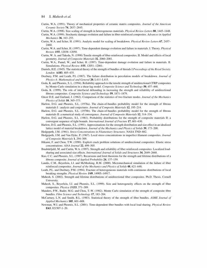
84 S. Mahesh et al.
Curtin, W.A. (1991). Theory of mechanical properties of ceramic matrix composites. Journal of the American
Ceramic Society 74, 2837–2845.
Curtin, W.A. (1998). Size scaling of strength in heterogeneous materials. Physical Review Letters 80, 1445–1448.
Curtin, W.A. (1999). Stochastic damage evolution and failure in fiber-reinforced composites. Advances in Applied
Mechanics 36, 163–253.
Curtin, W.A. and Scher, H. (1991). Analytic model for scaling of breakdown. Physical Review Letters 67, 2457–
2460.
Curtin, W.A. and Scher, H. (1997). Time-dependent damage evolution and failure in materials. I. Theory. Physical
Review B55, 12038–12050.
Curtin, W. A. and Takeda, N. (1998) Tensile strength of fiber-reinforced composites. II. Model and effects of local
geometry. Journal of Composite Materials 32, 2060–2081.
Curtin, W.A., Pamel, W., and Scher, H. (1997). Time-dependent damage evolution and failure in materials. II.
Simulations. Physical Review B55, 12051–12061.
Daniels, H.E. (1945). The statistical theory of the strength of bundles of threads I Proceedings of the Royal Society.
London A183, 405–435.
Duxbury, P.M. and Leath, P.L (1987). The failure distribution in percolation models of breakdown. Journal of
Physics A: Mathematical and General 20, L411–L415.
Goda, K. and Phoenix, S. L. (1994). Reliability approach to the tensile strength of unidirectional CFRP composites
by Monte-Carlo simulation in a shear-lag model. Composite Science and Technology 50, 457–468.
Goda, K. (1999). The role of interfacial debonding in increasing the strength and reliability of unidirectional
fibrous composites. Composite Science and Technology 59, 1871–1879.
Gücer D.E. and Gurland, J. (1962). Comparison of the statistics of two fracture modes. Journal of the Mechanics
Physics of Solids 10, 365–373.
Harlow, D.G. and Phoenix, S.L. (1978a). The chain-of-bundles probability model for the strength of fibrous
materials I : analysis and conjectures. Journal of Composite Materials 12, 195–214.
Harlow, D.G. and Phoenix, S.L. (1978b). The chain-of-bundles probability model for the strength of fibrous
materials II: a numerical study of convergence. Journal of Composite Materials 12, 314–334.
Harlow, D.G. and Phoenix, S.L. (1981). Probability distributions for the strength of composite materials II: a
convergent sequence of tight bounds. International Journal of Fracture 17, 601–630.
Harlow, D.G. and Phoenix, S.L. (1991). Approximations for the strength distribution and size effect in an idealized
lattice model of material breakdown. Journal of the Mechanics and Physics of Solids 39, 173–200.
Hedgepeth, J.M. (1961). Stress Concentrations in Filamentary Structures. NASA TND–882.
Hedgepeth, J.M. and Van Dyke, P. (1967). Local stress concentrations in imperfect filament composites. Journal
of Composite Materials 1, 294–309.
Hikami, F. and Chou, T.W. (1990). Explicit crack problem solutions of unidirectional composites: Elastic stress
concentrations. AIAA Journal 22, 499–505.
Ibnabdeljalil, M. and Curtin, W.A. (1997). Strength and reliability of fiber reinforced composites: Localized load-
sharing and associated size effects. International Journal of Solids and Structures 34, 2649–2668.
Kuo, C.C. and Phoenix, S.L. (1987). Recursions and limit theorems for the strength and lifetime distributions of a
fibrous composite. Journal of Applied Probability 24, 137–159.
Landis, C.M., Beyerlein, I.J. and McMeeking, R.M. (2000). Micromechanical simulation of the failure of fiber
reinforced composites. Journal of the Mechanics and Physics of Solids 48, 621–648.
Leath, P.L. and Duxbury, P.M. (1994). Fracture of heterogeneous materials with continuous distributions of local
breaking strengths. Physical Review B49, 14905–14917.
Mahesh, S. (2002). Strength and lifetime distributions of unidirectional fiber composites. Ph.D. Thesis. Cornell
University.
Mahesh, S., Beyerlein, I.J. and Phoenix, S.L. (1999). Size and heterogeneity effects on the strength of fiber
composites. Physica D133, 371–389.
Manders, P.W., Bader, M.G. and Chou, T.-W. (1982). Monte Carlo simulation of the strength of composite fibre
bundles. Fibre Science and Technology 17, 183–204.
McCartney, L.N. and Smith, R.L. (1983). Statistical theory of the strength of fiber bundles. ASME Journal of
Applied Mechanics 105, 601–608.
Newman, W.I. and Phoenix, S.L. (2001). Time-dependent fiber bundles with local load sharing. Physical Review
E63, 021507-1–20.
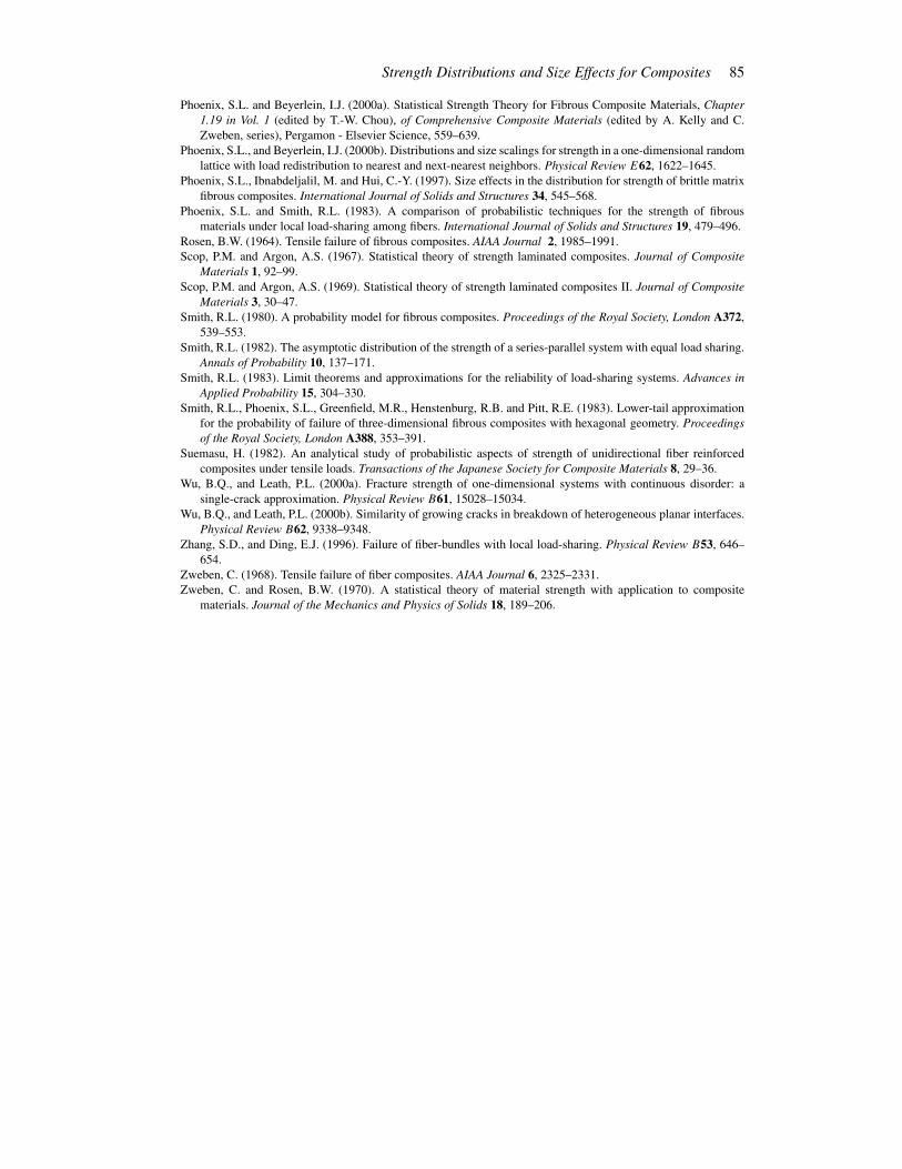
Strength Distributions and Size Effects for Composites 85
Phoenix, S.L. and Beyerlein, I.J. (2000a). Statistical Strength Theory for Fibrous Composite Materials, Chapter
1.19 in Vol. 1 (edited by T.-W. Chou), of Comprehensive Composite Materials (edited by A. Kelly and C.
Zweben, series), Pergamon - Elsevier Science, 559–639.
Phoenix, S.L., and Beyerlein, I.J. (2000b). Distributions and size scalings for strength in a one-dimensional random
lattice with load redistribution to nearest and next-nearest neighbors. Physical Review E62, 1622–1645.
Phoenix, S.L., Ibnabdeljalil, M. and Hui, C.-Y. (1997). Size effects in the distribution for strength of brittle matrix
fibrous composites. International Journal of Solids and Structures 34, 545–568.
Phoenix, S.L. and Smith, R.L. (1983). A comparison of probabilistic techniques for the strength of fibrous
materials under local load-sharing among fibers. International Journal of Solids and Structures 19, 479–496.
Rosen, B.W. (1964). Tensile failure of fibrous composites. AIAA Journal 2, 1985–1991.
Scop, P.M. and Argon, A.S. (1967). Statistical theory of strength laminated composites. Journal of Composite
Materials 1, 92–99.
Scop, P.M. and Argon, A.S. (1969). Statistical theory of strength laminated composites II. Journal of Composite
Materials 3, 30–47.
Smith, R.L. (1980). A probability model for fibrous composites. Proceedings of the Royal Society, London A372,
539–553.
Smith, R.L. (1982). The asymptotic distribution of the strength of a series-parallel system with equal load sharing.
Annals of Probability 10, 137–171.
Smith, R.L. (1983). Limit theorems and approximations for the reliability of load-sharing systems. Advances in
Applied Probability 15, 304–330.
Smith, R.L., Phoenix, S.L., Greenfield, M.R., Henstenburg, R.B. and Pitt, R.E. (1983). Lower-tail approximation
for the probability of failure of three-dimensional fibrous composites with hexagonal geometry. Proceedings
of the Royal Society, London A388, 353–391.
Suemasu, H. (1982). An analytical study of probabilistic aspects of strength of unidirectional fiber reinforced
composites under tensile loads. Transactions of the Japanese Society for Composite Materials 8, 29–36.
Wu, B.Q., and Leath, P.L. (2000a). Fracture strength of one-dimensional systems with continuous disorder: a
single-crack approximation. Physical Review B61, 15028–15034.
Wu, B.Q., and Leath, P.L. (2000b). Similarity of growing cracks in breakdown of heterogeneous planar interfaces.
Physical Review B62, 9338–9348.
Zhang, S.D., and Ding, E.J. (1996). Failure of fiber-bundles with local load-sharing. Physical Review B53, 646–
654.
Zweben, C. (1968). Tensile failure of fiber composites. AIAA Journal 6, 2325–2331.
Zweben, C. and Rosen, B.W. (1970). A statistical theory of material strength with application to composite
materials. Journal of the Mechanics and Physics of Solids 18, 189–206.


![Advances in Water Resources · using laser scanning confocal microscopy [37]. Pore- and throat-size distributions have also been obtained from analysis of 2D scanning electron microscopy](https://img.pdfslide.us/doc/110x75/5f08efb57e708231d4247165/advances-in-water-resources-using-laser-scanning-confocal-microscopy-37-pore-.jpg)