Embed Size (px)
Citation preview

STREAMING TECHNIQUES FOR
STATISTICAL MODELING
BY YIHUA WU
A dissertation submitted to the
Graduate School—New Brunswick
Rutgers, The State University of New Jersey
in partial fulfillment of the requirements
for the degree of
Doctor of Philosophy
Graduate Program in Computer Science
Written under the direction of
Prof. S. Muthukrishnan
and approved by
New Brunswick, New Jersey
October, 2007
ABSTRACT OF THE DISSERTATION
Streaming Techniques for Statistical Modeling
by Yihua Wu
Dissertation Director: Prof. S. Muthukrishnan
Streaming is an important paradigm for handling high-speed data sets that
are too large to fit in main memory. Prior work in data streams has shown
how to estimate simple statistical parameters, such as histograms, heavy hitters,
frequent moments, etc., on data streams. This dissertation focuses on a number
of more sophisticated statistical analyses that are performed in near real-time,
using limited resources.
First, we present how to model stream data parametrically; in particular, we
fit hierarchical (binomial multifractal) and non-hierarchical (Pareto) power-law
models on a data stream. It yields algorithms that are fast, space-efficient, and
provide accuracy guarantees. We also design fast methods to perform online
model validation at streaming speeds.
The second contribution of this dissertation addresses the problem of modeling
an individual’s behaviors via “signature” for nodes in communication graphs. We
develop a formal framework for the usage of signatures on communication graphs
and identify fundamental properties that are natural to signature schemes. We
justify these properties by showing how they impact a set of applications. We
ii

then explore several signature schemes in our framework and evaluate them on real
data in terms of these properties. This provides insights into suitable signature
schemes for desired applications.
Finally, the dissertation studies the detection of changes in models on data
with unknown distributions. We adapt the sound statistical method of sequen-
tial probability ratio test to the online streaming case, without independence
assumption. The resulting algorithm works seamlessly without window limita-
tions inherent in prior work, and is highly effective at detecting changes quickly.
Furthermore, we formulate and extend our streaming solution to the local change
detection problem that has not been addressed earlier.
As concrete applications of our techniques, we complement our analytic and
algorithmic results with experiments on network traffic data to demonstrate the
practicality of our methods at line speeds, and the potential power of streaming
techniques for statistical modeling in data mining.
iii

Acknowledgements
I would like to thank my advisor, Prof. S. Muthukrishnan, for his guidance
throughout my Ph.D. studies. Meeting with Muthu is alike to drink from a fire
hose, where it is so common for me to spend a week or longer unraveling the
new ideas (or suggestions) and key words from Muthu during a single one-hour
meeting. Muthu’s greatest gift as an advisor is to encourage me and to instill in
me the confidence in doing fun research on my own, without allowing me to settle
for doing less than the best I can. An excellent speaker himself, I learned from
Muthu how to give good talks, which I found extremely useful. On the other
hand, he is so effective in overcoming my anxiety, as a friend.
I am fortunate to have industrial collaborations with researchers from several
labs. These experiences are eye-openers to me, offering me a unique opportunity
to see how people outside universities do “real” work and do research. I am
grateful to Muthu for such hookups. I thank Flip Korn for being a thoughtful
mentor at AT&T Research. He helped me in every aspect. I benefited greatly
from many detailed discussions with him in many ways: in person, via emails and
on phone. His ideas and advice helped me find solutions to research problems
as well as the path to become a researcher. I am also thankful to Eric van den
Berg for his helpful advice on Chapter 5, to Graham Cormode for his consistent
interests in and encouragement to my work since my first research project. I am
very happy to have collaboration with Graham on Chapter 4.
I want to thank the remaining members of my thesis committee for their time
and interest in this dissertation. They are Prof. David Madigan, Prof. Richard
Martin, and Dr. Divesh Srivastava.
iv

I spent one summer at AT&T Research, as an intern. I enjoyed all my experi-
ences and I thank researchers there for spending time in talking about my work:
Tamraparni Dasu, Marios Hadjieleftheriou, Theodore Johnson, Yehuda Koren,
Shubho Sen, Oliver Spatscheck, Divesh Srivastava, Mikkel Thorup, Simon Ur-
banek, Suresh Venkatasubramanian, Chris Volinsky, and the fellow interns: Emi-
ran Curtmola, Bing Tian Dai, Irina Rozenbaum, Vladislav Shkapenyuk, Hang-
hang Tong, Ranga Vasudevan, Ying Zhang. I am also thankful to my friends and
fellow students in the department, who have made my time at Rutgers colorful.
Finally, I must thank my family members. Their love helped me through my
darker moods while in graduate school. Without their supports, none of this
would be possible.
v

Dedication
To my parents: Longcheng Wu and Sufang Xia. Without their selfless love, I
could not achieve anything.
vi

Table of Contents
Abstract . . . . . . . . . . . . . . . . . . . . . . . . . . . . . . . . . . . . ii
Acknowledgements . . . . . . . . . . . . . . . . . . . . . . . . . . . . . iv
Dedication . . . . . . . . . . . . . . . . . . . . . . . . . . . . . . . . . . . vi
List of Tables . . . . . . . . . . . . . . . . . . . . . . . . . . . . . . . . . xi
List of Figures . . . . . . . . . . . . . . . . . . . . . . . . . . . . . . . . xii
1. Introduction . . . . . . . . . . . . . . . . . . . . . . . . . . . . . . . . 1
2. Preliminaries . . . . . . . . . . . . . . . . . . . . . . . . . . . . . . . 8
2.1. Computational Model . . . . . . . . . . . . . . . . . . . . . . . . 8
2.1.1. Massive Data Streams . . . . . . . . . . . . . . . . . . . . 8
2.1.2. Window Models . . . . . . . . . . . . . . . . . . . . . . . . 9
2.1.3. Streaming Computational Model . . . . . . . . . . . . . . 10
2.1.4. Semi-Streaming Computational Model . . . . . . . . . . . 12
2.2. Streaming Analysis Tools . . . . . . . . . . . . . . . . . . . . . . . 12
2.2.1. Random Projections . . . . . . . . . . . . . . . . . . . . . 13
2.2.2. Sampling Techniques . . . . . . . . . . . . . . . . . . . . . 14
2.2.3. Other Algorithmic Techniques . . . . . . . . . . . . . . . . 15
3. Modeling Skew in Data Streams . . . . . . . . . . . . . . . . . . . 17
3.1. Introduction . . . . . . . . . . . . . . . . . . . . . . . . . . . . . . 17
3.2. Model Fitting on Data Streams . . . . . . . . . . . . . . . . . . . 20
3.3. Hierarchical (Fractal) Model . . . . . . . . . . . . . . . . . . . . . 22
vii

3.3.1. Model Definition . . . . . . . . . . . . . . . . . . . . . . . 22
3.3.2. Fractal Parameter Estimation . . . . . . . . . . . . . . . . 23
3.3.3. Model Validation . . . . . . . . . . . . . . . . . . . . . . . 27
3.4. Non-Hierarchical (Pareto) Model . . . . . . . . . . . . . . . . . . 30
3.4.1. Model Definition . . . . . . . . . . . . . . . . . . . . . . . 30
3.4.2. Pareto Parameter Estimation . . . . . . . . . . . . . . . . 30
3.4.3. Model Validation . . . . . . . . . . . . . . . . . . . . . . . 33
3.5. Fractal Model Fitting Experiments . . . . . . . . . . . . . . . . . 34
3.5.1. Alternative Streaming Methods . . . . . . . . . . . . . . . 34
3.5.2. Accuracy of Proposed Method . . . . . . . . . . . . . . . . 37
3.5.3. Comparison of Methods . . . . . . . . . . . . . . . . . . . 39
3.5.4. Performance On a Live Data Stream . . . . . . . . . . . . 40
3.5.5. Intrusion Detection Application . . . . . . . . . . . . . . . 44
3.6. Pareto Model Fitting Experiments . . . . . . . . . . . . . . . . . 45
3.6.1. Alternative Streaming Method . . . . . . . . . . . . . . . . 45
3.6.2. Accuracy of Proposed Method . . . . . . . . . . . . . . . . 46
3.6.3. Comparison of Methods . . . . . . . . . . . . . . . . . . . 48
3.7. Extensions . . . . . . . . . . . . . . . . . . . . . . . . . . . . . . . 49
3.8. Related Work . . . . . . . . . . . . . . . . . . . . . . . . . . . . . 51
3.9. Chapter Summary . . . . . . . . . . . . . . . . . . . . . . . . . . 53
4. Modeling Communication Graphs via Signatures . . . . . . . . 55
4.1. Introduction . . . . . . . . . . . . . . . . . . . . . . . . . . . . . . 55
4.2. Framework . . . . . . . . . . . . . . . . . . . . . . . . . . . . . . . 58
4.2.1. Individuals and Labels . . . . . . . . . . . . . . . . . . . . 58
4.2.2. Signature Space . . . . . . . . . . . . . . . . . . . . . . . . 59
4.2.3. Signature Properties . . . . . . . . . . . . . . . . . . . . . 61
viii
4.2.4. Applying Signatures . . . . . . . . . . . . . . . . . . . . . 63
4.3. Example Signature Schemes . . . . . . . . . . . . . . . . . . . . . 64
4.3.1. One-hop Neighbors Based Approaches . . . . . . . . . . . 66
4.3.2. Multi-hop Neighbors Based Approach . . . . . . . . . . . . 68
4.4. Evaluations of Signature Properties . . . . . . . . . . . . . . . . . 70
4.4.1. Data Sets . . . . . . . . . . . . . . . . . . . . . . . . . . . 71
4.4.2. Distance Functions . . . . . . . . . . . . . . . . . . . . . . 72
4.4.3. Experimental Results . . . . . . . . . . . . . . . . . . . . . 73
4.5. Application Evaluation . . . . . . . . . . . . . . . . . . . . . . . . 78
4.6. Extensions . . . . . . . . . . . . . . . . . . . . . . . . . . . . . . . 81
4.7. Related Work . . . . . . . . . . . . . . . . . . . . . . . . . . . . . 83
4.8. Chapter Summary . . . . . . . . . . . . . . . . . . . . . . . . . . 83
5. Modeling Distributional Changes via Sequential Probability Ra-
tio Test . . . . . . . . . . . . . . . . . . . . . . . . . . . . . . . . . . . . . 85
5.1. Introduction . . . . . . . . . . . . . . . . . . . . . . . . . . . . . . 85
5.2. Change Detection Problems . . . . . . . . . . . . . . . . . . . . . 87
5.3. Our Global Change Detection Algorithms . . . . . . . . . . . . . 89
5.3.1. Preliminary . . . . . . . . . . . . . . . . . . . . . . . . . . 89
5.3.2. Our Offline Algorithm . . . . . . . . . . . . . . . . . . . . 91
5.3.3. Streaming Algorithm . . . . . . . . . . . . . . . . . . . . . 93
5.4. Our Local Change Detection Algorithms . . . . . . . . . . . . . . 97
5.5. Global Change Detection Experiments . . . . . . . . . . . . . . . 100
5.5.1. Experiment Setup . . . . . . . . . . . . . . . . . . . . . . . 100
5.5.2. Efficacy of Proposed Methods . . . . . . . . . . . . . . . . 101
5.5.3. Comparison of Methods . . . . . . . . . . . . . . . . . . . 103
5.5.4. Applications . . . . . . . . . . . . . . . . . . . . . . . . . . 105
ix

5.6. Local Change Detection Experiments . . . . . . . . . . . . . . . . 108
5.7. Related Work . . . . . . . . . . . . . . . . . . . . . . . . . . . . . 112
5.8. Chapter Summary . . . . . . . . . . . . . . . . . . . . . . . . . . 114
6. Conclusions and Future Work . . . . . . . . . . . . . . . . . . . . . 115
Curriculum Vita . . . . . . . . . . . . . . . . . . . . . . . . . . . . . . . 130
x
List of Tables
3.1. Estimates of b on synthetically generated data. . . . . . . . . . . . 37
3.2. Some statistics from Gigascope experiments. . . . . . . . . . . . . 43
3.3. Estimates of z on synthetically generated data. . . . . . . . . . . 46
4.1. Different applications and their requirements . . . . . . . . . . . . 63
4.2. Communication Graph Characteristics and Properties . . . . . . . 66
4.3. Properties Used by Signature Schemes . . . . . . . . . . . . . . . 70
4.4. Performance on signature persistence and uniqueness . . . . . . . 75
4.5. Summary of the relative behaviors of the signature schemes . . . . 78
xi
List of Figures
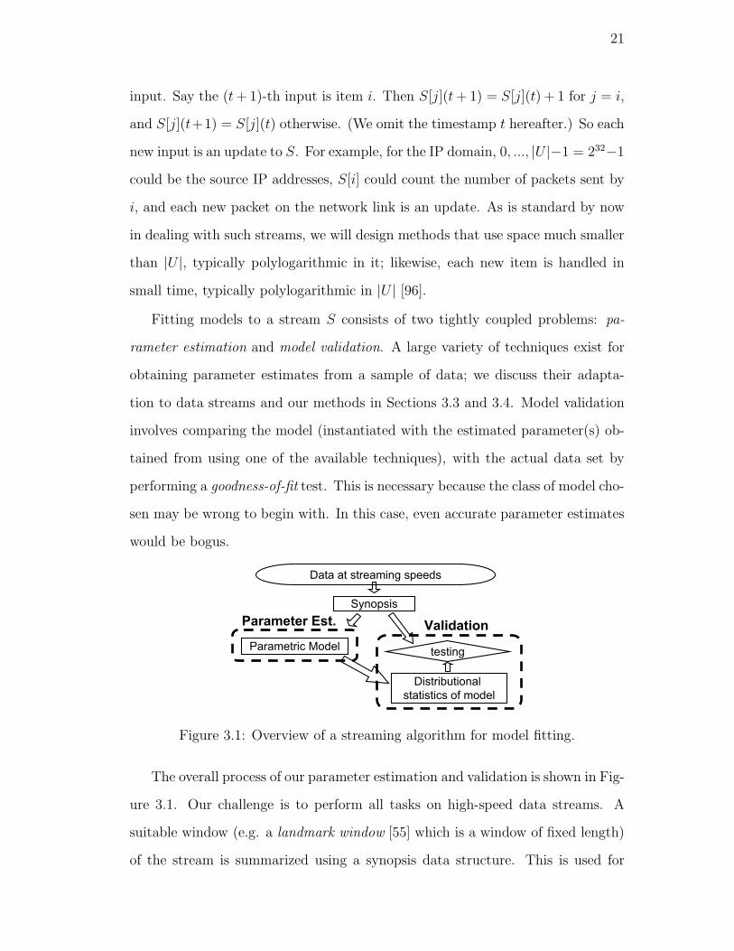
3.1. Overview of a streaming algorithm for model fitting. . . . . . . . . 21
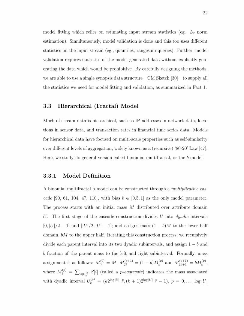
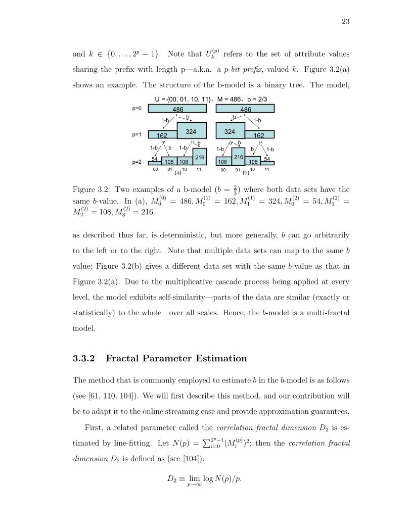
3.2. Two examples of a b-model (b = 23) where both data sets have the
same b-value. In (a), M(0)0 = 486, M
(1)0 = 162, M
(1)1 = 324, M
(2)0 =
54, M(2)1 = M
(2)2 = 108, M
(2)3 = 216. . . . . . . . . . . . . . . . . . 23
3.3. Computing D2 for the example in Figure 3.2. . . . . . . . . . . . . 24
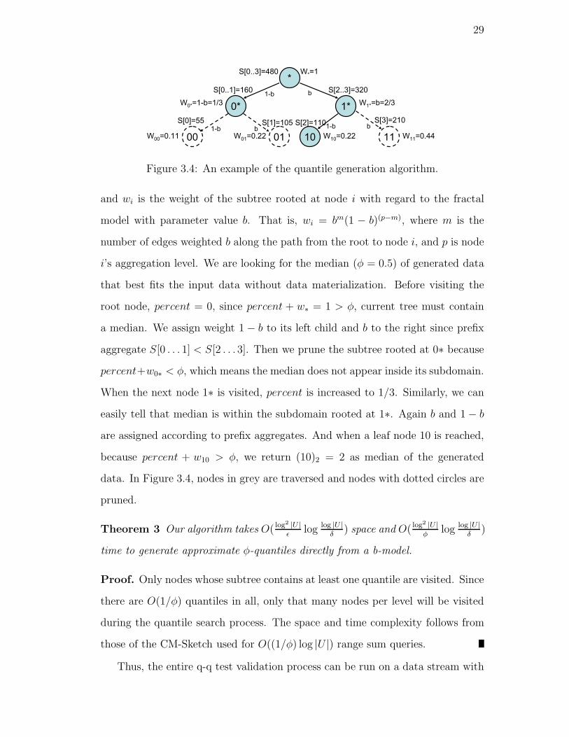
3.4. An example of the quantile generation algorithm. . . . . . . . . . 29
3.5. CCDF plot of fitted Pareto for HTTP connection sizes . . . . . . 31
3.6. An example of pyramid approximation. . . . . . . . . . . . . . . . 36
3.7. Algorithm evaluation: accuracy and running time of online and
offline fractal model fitting, at per-minute time intervals. . . . . . 38
3.8. Algorithm comparison: accuracy and running time of various al-
gorithms, as a function of the number of levels. . . . . . . . . . . 38
3.9. Performance and Study of Stability and Fit of Models on Gigas-
cope: b-values, correlation coefficients. (a) TCP data on destIP;
(b) TCP data on srcIP. . . . . . . . . . . . . . . . . . . . . . . . . 41
3.10. Model Fitting on IP Traffic Data with Network Intrusion Attacks 44
3.11. Performance of parameter estimation. . . . . . . . . . . . . . . . . 47
3.12. Algorithm comparison. . . . . . . . . . . . . . . . . . . . . . . . . 48
3.13. Algorithm comparison: accuracy and running time of offline and
online D0, at per-minute time intervals. . . . . . . . . . . . . . . . 50
4.1. Popularity of nodes in signatures. . . . . . . . . . . . . . . . . . . 73
4.2. Signature persistence and uniqueness on two real data sets. . . . . 74
xii

4.3. ROC curves from network data . . . . . . . . . . . . . . . . . . . 75
4.4. Signature Robustness on Network Data . . . . . . . . . . . . . . . 77
4.5. Multiusage detection: ROC curves . . . . . . . . . . . . . . . . . 79
4.6. Performance of label masquerading detection. . . . . . . . . . . . 81
5.1. Examples of local and global changes. P0 and P1 are respective
probability density function (or PDF) of pre- and post-change dis-
tributions. . . . . . . . . . . . . . . . . . . . . . . . . . . . . . . . 89
5.2. An illustration for the sequential change detection algorithm. . . . 93
5.3. Sketch structure for EH+CM. . . . . . . . . . . . . . . . . . . . . 95
5.4. Change detection accuracy. . . . . . . . . . . . . . . . . . . . . . . 102
5.5. Accuracy for global change point estimates and detection delays. . 103
5.6. Normalized detection delays(
|n−w|w
)
of various methods. . . . . . 105
5.7. Accuracy to answer queries on post-change distributions: EHCM
vs. FSWIN . . . . . . . . . . . . . . . . . . . . . . . . . . . . . . 107
5.8. Accuracy of detected local changes. . . . . . . . . . . . . . . . . . 109
5.9. Accuracy for local change-point estimates and detection delays. . 111
xiii
1
Chapter 1
Introduction
Database research has sought to scale management, processing and mining of data
sources to ever larger sizes and faster rates of transactions. One of the challenging
applications is that of data streams where data sizes are so large that it is difficult
to store all of the data in a database management system (DBMS) and there
may be millions of “transactions” per second. We describe some quintessential
examples as follows:
• Wireless sensor networks are ubiquitous [44, 118]. Sensor networks are used
for location tracking [116], geophysical monitoring [118, 88], “communities”
identification [108] thereof.
• There are multiple information and social networks among internet users,
from web (e.g., blog) to chat networks (e.g., instant message (IM)). Given
the trend in the expansion of information systems and the development of
automatic data-collecting tools, data sets we will encounter in the future
are expected to be more “massive” than what we have today.
• The volume of transaction log data generated is overwhelming. For example,
there are approximately 3 billion telephone calls in U.S. every day, 30 billion
emails daily. By comparison, the amount of data generated by world-wide
credit card transactions is very small, at only 1 billion per month [94].
• In the networking community, there has been a great deal of interest in
analyzing IP traffic data where the packets and flows (“connections”) get
2
forwarded in high speed links [38]. Traffic monitoring ranges from the long
term (e.g., monitoring link utilizations) to the ad-hoc (e.g., detecting net-
work intrusions). Many of the applications operate over huge volumes of
data (Gigabit and high-speed links), and have real-time reporting require-
ments.
In all above examples, data takes the form of continuous data streams rather
than finite stored data sets, and long-running continuous queries are needed, as
opposed to one-time queries. Traditional database systems and data processing
algorithms are ill-equipped to handle complex and numerous continuous queries
over data streams, and many aspects of data management and processing need to
be reconsidered in their presence. Therefore, the research community has devel-
oped a large body of work in data stream management systems (DSMSs). Systems
developed at various universities of this type include Aurora [4], STREAM [1] and
TelegraphCQ [23], etc. Additional systems in this category are also developed in
research labs like AT&T (Gigascope) [37], Sprint (CMON) [2], Telcordia [25].
Moreover, the academic system Aurora has given rise to the commercial Stream-
Base Systems Inc. [3] 1.
Prior work in data stream has shown how to estimate simple statistics such as
distinct counts [51, 11, 34, 56, 58]), summary aggregates (e.g., heavy hitters [30,
24, 91], quantiles [63, 92, 30], histograms [65, 64, 60], wavelets [22]) and query
results [30, 32, 7] (e.g., inner product, frequency moments). We need vastly more
sophisticated statistical analyses in data stream models, which constitute the
focus of this dissertation — statistical modeling of streaming data.
For statistical modeling of input data, we have three fundamental questions
to address:
1. Model fitting — How to find parameters that make a model fit the data as
1http://www.streambase.com

3
closely as possible (given some assumptions)?
2. Model validation — How precise are the best-fit parameter values? Would
another model be more appropriate?
3. Change detection — How to detect a change in models?
Model fitting and model validation are closely related. No matter there is a
change in the underlying model or not, it is necessary for model validation to
justify the correctness of the class of model chosen to begin with. If we start
with a wrong model, even accurate model fitting is meaningless. Additionally,
when modeling streaming data, the computational issue with regard to the three
questions efficiently arises.
Generally speaking, developing a model of the underlying data source leads to
a better understanding of the source and its characterization, which can lead to
a number of applications in query processing and mining. For example, in sensor
systems, models are found effective in offering noise resilient answers to a wide
variety of queries (e.g., selectivity estimation [46], nearest neighbor queries [16,
100], and similarity searches [16], etc.) with much less network bandwidth usage
by acquiring data only when it is not sufficient to approximate query answers with
acceptable confidence [44, 42]. Models are also useful for trend analysis [103].
Once we have established a reliable model of “normal” behavior, then anomalies
and trend changes, defined as deviations to the model, can be detected, we thus
trigger actions or alarms.
We investigate two representative categories of modeling in data streams in
this dissertation: parametric and structural modeling.
In statistics, a parametric model is a parametrized family of probability dis-
tributions, which describe the way a population is distributed. Assuming a model
for the input stream, the goal of parametric modeling is to estimate its parame-
ter(s) using one of the well-known methods such as regression fitting, maximum
4
likelihood estimation, expectation maximization and Bayesian approach on the
data stream models. Due to the ubiquity of skew in data, as we can see in IP
network [81, 113], financial [52], sensor [44], and text streams [32, 89] etc., we
are particularly interested in modeling skew 2 in data streams. The challenges
to do parametric model fitting at streaming speeds are both technical — how to
continually find fast and reliable parameter estimates on high speed streams of
skewed data using small space — and conceptual — how to validate the goodness-
of-fit and stability of the model online. We show how to fit two models of skew
— hierarchical (binomial multifractal) and non-hierarchical (Pareto) power-law
models — on a data stream.
From another perspective, many real applications can be modeled using com-
munication graphs where interested persons engage in various activities such as
telephone calls, emails, Instant Messenger (IM), blog, web forum, e-business and
so on. These arise in applications in characterizing an individual’s communica-
tion behaviors, identifying repetitive fraudsters, message board aliases, extremists
etc., using structural information described by graphs. Thus we call it structural
modeling. Tracking such electronic identities on communication networks can be
achieved if we have a reliable “signature” for nodes and activities. In particu-
lar, a signature for a node is a subset of graph nodes that are most relevant to
the query node, such that the signature represents the query node’s communica-
tion patterns. While many examples of signatures can be proposed for particular
tasks [36, 70, 69], what we need is a systematic study of the principles behind the
usage of signatures to any task. Our framework on signatures for communication
graphs addresses this challenge and the scalability issues with respect to signature
schemes.
2In particular, we are modeling skew in frequencies of domain values. So here “skew” meansfew item values are frequent, and we observe a long tail of infrequent values.
5
Another problem of interest, in parallel with modeling, in monitoring streams
of data in a broad range of application is that of change detection [53, 72, 111].
A change in the data source can cause the models stale and degrade their accu-
racy, so a change detection system should respond promptly to a change when
it happens. Parametric change detection methods [44, 42, 82] trigger an alarm
when there is a significant change in parameter value(s). But real data often
does not obey simple parametric distributions in practice. Therefore we need a
non-parametric technique that makes no assumptions on the form of the distri-
bution as a priori. To the best of our knowledge, prior approaches in database
research to detecting a change in non-parametric distributions affix two windows
to streaming data and estimate the change in distribution between them [39, 80].
Fixing a window size is problematic when the information on the time-scale of
change is unavailable, and it is infeasible to exhaustively search over all possible
window sizes either. We improve existing work by adapting the statistically sound
sequential probability ratio test [109] to the online streaming case for change de-
tection, such that the most likely change-point estimate is integrated into the test
statistics, then changes at different scales can be detected without instantiating
windows of different sizes in paralle.
Since the IP traffic analysis case is the most developed application for data
streaming, we focus on network traffic data for application study of our proposed
techniques. The contributions of this dissertation are as follows:
• Parametric modeling. (Chapter 3) We show how to fit hierarchical (bi-
nomial multifractal) and non-hierarchical (Pareto) power-law models on a
data stream. We address the technical challenges using an approach that
maintains a sketch of the data stream and fits least-squares straight lines; it
yields algorithms that are fast, space-efficient, and provide approximations
of parameter value estimates with a priori quality guarantees relative to
those obtained offline. We address the conceptual challenge by designing

6
fast methods for online goodness-of-fit measurements on a data stream; we
adapt the statistical testing technique of examining the quantile-quantile
(q-q) plot, to perform online model validation at streaming speeds.
We complement our analytic and algorithmic results with experiments on IP
traffic streams in AT&T’s Gigascope R© data stream management system,
to demonstrate practicality of our methods at line speeds. We measured the
stability and robustness of these models over weeks of operational packet
data in an IP network. In addition, we study an intrusion detection appli-
cation, and demonstrate the potential of online parametric modeling.
• Structural modeling. (Chapter 4) We develop a formal framework for the
use of signatures on communication graphs and identify three fundamental
properties that are natural to signature schemes: persistence, uniqueness
and robustness. We justify these properties by showing how they impact a
set of applications. We then explore several signature schemes — previously
defined or new — in our framework and evaluate them on real data in
terms of these properties. This provides insights into suitable signature
schemes for desired applications. As case studies, we focus on the concrete
application of enterprise network traffic. We apply signature schemes to two
real problems, and show their effectiveness. Finally, we discuss scalability
issues with respect to signature schemes.
• Change detection. (Chapter 5) We adopt the sound statistical method of
sequential hypothesis testing to study the problem of change detection on
streams, without independence assumption. It yields algorithms that are
fast, space-efficient, and are oblivious to data’s underlying distributions.
Additionally, we formulate and extend our methodology to local change
detection problems that have not been addressed earlier. We perform a
thorough study of these methods in practice with synthetic and real data

7
sets to not only determine the existence of a change, but also the point
where the change is initiated, with only a small delay between the change
point and the ponit when it is detected. Our methods work seamlessly
without window limitations inherent in prior work, and are highly effective
at detecting changes quickly as our experiments show.
8
Chapter 2
Preliminaries
2.1 Computational Model
2.1.1 Massive Data Streams
A data stream is a sequence of data elements x1, x2, . . . , xn from a data source,
with xi ∈ U = {0 . . . u − 1}. The semantics of the data element xi may be
different from application to application. This leads to different models of data
streams. Each data element xi may represent a number such as, an IP address, a
telephone number, a student ID, and the ID of an item in transaction, etc. It may
also represent an instance of interaction or communication between individuals;
that is, xi = (si, di) denotes an interaction between si and di. Moreover, xi can
be attached with more sophisticated data semantics; for example, each xi may
represent a subset of the items that customers put in their market baskets for one
transaction. With such a data stream, the input is also time series, where the
ith entry in the sequence is a measurement at time i. In this dissertation, when
referring to streams, we mean a data stream like the above one, and we do not
consider streams where data might arrive out of (time) order.
There is another type of data stream [96], in which an implicit array S of
domain size u is involved. Here S[i] is the value of the ith entry of array S, and
denotes the total for item i ∈ U in the stream. Data elements in the stream may
take the form (i, k), where i ∈ U and k ∈ Z. The semantics of such an element
state that S[i] = S ′[i] + k, where S[i] and S ′[i] are respective value of that entry

9
after and before seeing the element. This leads to streaming models such as the
cash-register model and the Turnstile model [96]. The difference between the two
models is that, in the cash-register model k ≥ 0; while in the Turnstile model, k
could be negative.
All streaming problems considered in this dissertation assume that data ele-
ments are only added to the current set, but not deleted. This is because models
with the full dynamic property are orthogonal to our proposed methodologies, so
we do not consider those variants for now.
2.1.2 Window Models
A good model for streaming data should fit well on many subsets (window of data)
to be considered robust. Due to the evolution of the real data, it is inaccurate
to build models over the entire data stream. It is natural to imagine that the
recent past in a data stream is more significant than the distant past. There are
a variety of streaming windows to emphasize the data from the recent past:
• Landmark windows [55, 119] identify certain timepoints called landmarks
in the data stream, and the aggregate value at a point is defined with respect
to the data elements from the immediately-proceeding landmark k until the
current point. A cumulative window is a special case when k = 1; in this
case, all the available data are considered. An example of a landmark is
when a user requests the computation of an ad hoc query.
• Sliding windows [40] are typically of a fixed size. One specifies a window
size w, and explicitly focuses only on the most recent stream of size w. That
is, at time n, only consider a sliding window of updates xn−w+1, . . . , xn.
Elements outside this window fall out of consideration for analysis, as the
window slides over time.

10
• Decaying window [27] model believes that recent sliding windows are
more important than previous ones, with weights of data from one window
decreasing exponentially into the past. Formally, one considers the signal
as fixed size windows of size w and the aging factor λ. Let Bi represent the
signal from window i. We inductively maintain βi as the meta-signal after
seeing i windows. When the (i + 1)th window is seen, we obtain
βi+1 = (1− λ)βi + λBi+1.
This weight function provides a smooth dynamic evolution of βi+1. In ad-
dision, periodic updates do not require accessing transaction data for all
previous time windows. All that is needed is βi and the new set of transac-
tions defined by Bi+1.
Ideally, we like methods to work on all of these window models so that we can
flexibly try modeling the data in different ways.
2.1.3 Streaming Computational Model
A data stream contains large volume of data, but what makes data streams unique
is the very large universe. For example, the universal size could be
• the number of distinct source, destination IP address pairs, which could be
as large as 264 in the IPv4 domain;
• the number of distinct http addresses on the web, which is potentially infi-
nite since web queries get sometimes written into http headers;
• the size of a cross-product of the domains of the attributes of interest. This
may lead to a potentially large domain space even if individual attribute
domains are small.

11
A streaming algorithm is an algorithm that computes some function over a
data stream at different times. These functions can be thought of as queries to
the data structure updated during the stream. Due to the explosion of data, a
desired streaming algorithm satisfies the following properties:
• Storage. All elements observed on the fly should be summarized in a
synopsis structure [57] with space much smaller than the domain size u,
typically polylogarithmic in it.
• Per-item processing time. Synopsis should be fast to update in order to
match the streaming speeds. As is standard in dealing with data streams,
each new element is handled in small time, typically polylogarithmic in u.
• Query time. Based on a synopsis of original data, functions on the in-
put stream should be computed efficiently and preferrably with accuracy
guarantees, provided a priori, so that queries can be evaluated on-demand
frequently.
• One pass, sequential access. The input stream is accessed in a sequential
fashion. The order of the data elements in the stream is not controlled by
the algorithm. Moreover, it is preferrable for the algorithm to evaluate
functions over the stream in one or at most a small number of passes.
These properties characterize the algorithm’s behaviors during the time when it
goes through the input data stream. The algorithm may perform certain pre-
processing and/or post-processing on the workspace (not on the input stream)
before and/or after this time.
Property 1 [96] At any time n in the data stream, we would like the per-item
processing time, storage as well as the computing time of a streaming algorithm to
be simultaneously o(u, n), preferrably, polylog(u, n), where u is the domain size.

12
2.1.4 Semi-Streaming Computational Model
Consider the spectrum of the size of the storage space that an algorithm takes to
access the input data. At one extreme of the spectrum, we have algorithms that
can use memory large enough to hold the whole input. At the other extreme,
we have streaming algorithms that use only polylogarithmic space. It has been
suggested in [96] a middle ground:
Property 2 [96] With the semi-streaming model, for a graph with n vertices,
the algorithms use O(n · polylog(n)) bits of space.
That is, the space is proportional to n, the number of vertices, and sublinear in
m, the number of edges. Some interesting results have been obtained in the semi-
streaming model for graph properties such as diameters, spanners etc. [50, 49]. We
consider this model in structural analysis of communication graphs for signatures
(see Chapter 4).
2.2 Streaming Analysis Tools
Previous work on streaming algorithms has focused on computing statistics over
the stream. In a data stream setting, with small-space data structures that can
be updated for each input every efficiently, such algorithms cannot solve most
problems on input exactly, so we will allow approximations. In fact, all algorithms
we show will be probabilistic and will succeed with probability at least 1− δ and
be accurate to some prespecified error ǫ, for parameters ǫ and δ. We discuss below
the main mathematical and algorithmic techniques used in data stream models
that serve as basic building blocks in solving our problems.
13
2.2.1 Random Projections
Random projection is a simple geometric technique for reducing the dimension-
ality, using projection along pseudo-random vectors. The pseudo-random vectors
are generated by space-efficient computation of limitedly independent random
variables. These projections are called the sketches. Many sketches have been
proposed in DSMSs, each suitable of different sets of problems and with different
time and space requirements [9, 96].
Count-Min (CM) Sketch [30, 32] is a small-space data structure that is useful
for variety of approximations. It has similar performance as the best-known
sketches [7, 24, 28, 74] in terms of accuracy for estimates we care about, but has
the best update time.
The CM sketch with parameters (ǫ, δ) is a two dimensional array of counters
with width l and depth d = ⌈ln 1δ⌉: count[1, 1] . . . count[d, l]. Each entry of the
array is initially zero. Additionally, d hash functions h1 . . . hd : U → {1 . . . l} are
chosen uniformly at random from a pairwise-independent family. Given l and d,
the space overhead is the ld counters and the d hash functions, each of which can
be stored using two words. Whenever an update (it, ct) arrives (e.g., tth packet
with source it and bytesize ct), ct is added to only one count in each row, and the
counter is determined by hj. Formally, we set
∀1 ≤ j ≤ d : count[j, hj(it)]← count[j, hj(it)] + ct.
The update time depends on the depth d of the sketch. CM sketch can be used
to answer a variety of queries. The output procedure varies with the application
as well as the choice of sketch width l.
Fact 1 With probability at least 1− δ, CM-Sketch [30, 32] provides ǫ approxima-
tions to point, rangesum, inner-product queries, L2-norm and quantile esitmations
14
in small — typically O( log2 |U |ǫ2
log( log |U |δ
)) — space and per-item update time 1.
Estimating number of distinct elements. This is a fundamental problem
in data streams, and several approaches [11, 34, 51, 56, 58] have been proposed
to approximate the number of distinct elements observed. We omit detailed
discussions of these methods, and summarize the properties that they guarantee:
Fact 2 There exist approximate distinct counter algorithms [51, 11] that take
parameters ǫ and δ and create a data structure of size O( 1ǫ2
log 1/δ) machine
words. The time to process each update is O(log 1/δ). For an input stream of
(integer) values, such algorithms report an estimate d for the distinct count such
that, if d is the true number of distinct elements observed, then with probability
at least 1− δ, (1− ǫ)d ≤ d ≤ (1 + ǫ)d.
2.2.2 Sampling Techniques
Sampling in the data stream context means every data element is seen but only a
(polylogarithmic sized) subset of them are retained. Which subset of elements to
keep can be chosen deterministically or in a randomized way. Various sampling
algorithms have been proposed to estimate quantiles [63, 105], to find frequent
elements [91], to estimate the inverse distribution [33], and to find rangesum of
elements [6] in a data stream. But the worst case query cost of any sampling
algorithm that (ǫ, δ)-approximates inner-product queries and L2 norm — queries
we care about — is more expensive than the cost for sketches with the same
accuracy guarantees [10]. Therefore, we do not consider sampling algorithms in
the rest of this dissertation.
1Here, we have given a general upper bound that applies to the estimation of all the aggregates.
In the remainder of the dissertation, we will provide bounds for various tasks that are specific
to only the aggregates the tasks need.

15
2.2.3 Other Algorithmic Techniques
Exponential Histograms (EHs) [40] are used to estimate all data counts in a
recent window of size W . Datar et al provided tight bounds where log2 n bits
are sufficient and necessary for (1 + ǫ) approximate estimates at time n. EH
maintains buckets over ranges of data points. All data (it, ct) seen in a time range
t ∈ (ti−1, ti] are aggregated into the ith bucket, and the EH maintains the value
ti and the count Ci =∑
ti−1<t≤tict for each bucket. Buckets where ti < n −W
are discarded. When a new data point arrives, it is placed in its own new bucket.
Buckets are then merged in a certain way such that there is always a logarithmic
O(log n) number of buckets. At any given point n, the count estimate on the
most recent W observations can be obtained from∑
i Ci.
A characterization of the merging process of EH is that two consecutive buck-
ets are merged if the combined count of the merged buckets is dominated by the
total count of all more-recent buckets. A merger of more-recent buckets may lead
to a cascade of at most O(log n) such mergers of less-recent buckets upon the
arrival of a single new element. But the amortized number of mergers is O(1)
per new item. Furthermore, the sequence of bucket counts (from the most- to the
least-recent) is a non-decreasing sequence of powers of 2, and for some k = Θ(1/ǫ)
and some P ≤ log 2nk
+ 1, for each possible count 2p < 2P , there are exactly k or
k + 1 buckets having count 2p, there are at most k + 1 buckets having count 2P ,
and no buckets have counts greater than 2P .
Union Bounds [95]. This is very frequently used in streaming analysis. It
derives directly from the inclusion-exclusion principle and states that the proba-
bility of the union of a set of events is at most the sum of the probabilities of the
events. Formally, let E1, E2, . . . , En be an arbitrary set of events, the bound says:
Pr(∪ni=1Ei) =
∑
i
Pr(Ei)−∑
i<j
Pr(Ei ∩ Ej) + · · · ≤∑
i
Pr(Ei).
An important feature of the union bound is that there is no other condition on the

16
events for the bound to hold. In particular, when the events are not independent,
the bound still holds. This is quite useful in places where independence among
random variables cannot be achieved.
17
Chapter 3
Modeling Skew in Data Streams
3.1 Introduction
While much of prior work on data stream analysis has focused on nonparametric
techniques such as approximate aggregates (e.g., heavy hitters, distinct counts),
summaries (e.g., quantiles, histograms, wavelets) and query results (e.g., join
sizes)—see [9, 96] for surveys—little effort has been focused on modeling the data
stream parametrically. In general, developing a model of the underlying data
source leads to a deeper structural insight into the source and its characterization,
which can lead to a number of applications in query processing and data mining.
For example, parametric models are used in selectivity estimation [46], trend
analysis [103], outlier detection [101], and improving the quality guarantees of
existing algorithms [32, 87]. Models are also useful for generating synthetic traces
of data sources for experimental or simulation studies [110], model-driven data
acquisition in sensor networks [43] and provisioning [113].
What are suitable models for data streams? There are suitable hierarchical
as well as non-hierarchical models.
Data streams have hierarchical dimensions, such as IP addresses in network
data, locations in sensor data, and time indexed share volumes in financial streams.
Models for hierarchical data have focused on multi-scale properties over different
levels of aggregation. Recently, in the networking community, the IP address
space has been shown to be well modeled using the fractal dimension [81]. Using
a variety of traces of network traffic, the authors considered the fractal dimension
18
of the traffic over the IP address space, and showed it is (a) stable over short time
intervals at local sites; (b) different at different sites with different characteristics;
and (c) different with changes in traffic conditions such as during a worm attack.
Hence, it is possible that the fractal dimension of the IP address distribution can
serve as a “fingerprint” for normal traffic, and that sudden deviations from this
would signal an anomaly or a change in network trends.
At a non-hierarchical view, streaming data is also teeming with high variability—
most observations take small values, while a few observations attain extremely
large values with non-negligible probabilities. This phenomena is ubiquitous in in-
ternet traffic—IP flow sizes, TCP connection duration, request interarrival times,
node degrees of inferred Autonomous System, and file sizes transferred over the
Internet; see [112] for references. All these are well modeled by heavy-tailed—
in particular, Pareto—distributions and are characterized by (non-hierarchical)
skew. Moreover, Pareto/power-law modeling of financial streams of stock prices
and number of trades is useful for real-time forecasting and options pricing [52].
What are the revelant issues in fitting models to streaming data? Typically,
model fitting is done offline when it applies to stable situations where it is done
once or infrequently, such as in [81, 112]. However, the dynamics of streaming
data calls for continuous parameter estimation and validation of models to find
reliable models that are robust over long time intervals. For example, at any time
an unnoticed DDoS attack may be altering the distribution of IP address prefixes
in the traffic; this is not a rare occurrence in actual measurement studies [83].
This suggests the need for a higher threshold for accepting a model, to reduce its
susceptibility to outliers by demonstrating temporal stability. In a data stream
context such as IP traffic modeling, it is impractical to gather data frequently
and perform offline analyses. The preferred approach is to perform estimation on
the data stream directly as the data is generated. It is therefore imperative that
estimation work at line speeds (i.e., rates at which packets are forwarded in the

19
links). As a consequence, there are two outstanding concerns in modeling data
streams:
1. How to estimate the model parameter(s) on data streams? Well known
statistical tools such as EM [62] are both computationally expensive and
require a large amount of storage to provide accurate estimates, and are
therefore infeasible within the space and time constraints of a Data Stream
Management System (DSMS).
2. How to validate the goodness-of-fit of the model with the estimated pa-
rameter(s) on data streams? Using traditional statistical hypothesis testing
techniques is typically infeasible within the space and time constraints of a
DSMS.
These concerns are broadly applicable to all modeling applications. We ad-
dress these concerns and present methods for hierarchical and non-hierarchical
modeling in data streams. Our contributions are as follows:
• To the best of our knowledge, this is the first work on model fitting over
data streams with a priori error guarantees. We show how to maintain an
estimate of the binomial multifractal (“b-model”) and Pareto model param-
eters using few memory updates per item and small space; our algorithm
provably output parameter estimates to within an additive error bound that
can be prespecified.
• We present highly efficient streaming methods to validate the model param-
eters online using quantile-quantile (“q-q”) plots from statistics, which are
widely used for power-law fitting. This requires computing order statistics
of the ideal models: we propose methods to compute them without actually
generating data, which would be prohibitive on a data stream.
20
• We complement our analytical and algorithmic results with a detailed ex-
perimental study on a variety of real IP traffic data streams from AT&T. In
particular, we have implemented our methods within the Gigascope system
that is operational inside the AT&T network, to perform model fitting at
speeds of 100K packets per second using only 2% of CPU utilization. We
ran this experiment over a period of several weeks to measure the robustness
and stability of the model. We also perform a detailed study of applicabil-
ity of modeling to an application—intrusion detection—with labeled data.
These real-data experiments provide many insights into the fit of models
on packet-level data and their applicability, something that could not have
been possible without our proposed streaming solutions. As our experience
shows, prior offline trace-driven study provides only limited insight into the
applicability of model that fit IP streams, and careful interpretation of the
evolution of the model parameters as well as the quality of fit of the model
are needed to reason about streaming data.
The chapter is organized as follows. We present a high level view of our
approach in Section 3.2. We present our algorithmic solutions for modeling and
validating (hierarchical) b-model in Section 3.3 and present experimental studies
in Section 3.5. Likewise, we present algorithmic methods and experimental studies
in Sections 3.4 and 3.6 respectively for (non-hierarchical) Pareto model fitting and
validation. Our overall approach can be extended to other models and streaming
applications quite naturally. Section 3.7 describes these extensions. Related work
is in Section 3.8 and conclusions are in Section 3.9.
3.2 Model Fitting on Data Streams
Let U = {0, ..., |U |−1} be the data domain. Our goal is to model the distribution
S[0, . . . , |U | − 1](t) where S[i](t) is the frequency of item i after seeing the t-th
21
input. Say the (t + 1)-th input is item i. Then S[j](t + 1) = S[j](t) + 1 for j = i,
and S[j](t+1) = S[j](t) otherwise. (We omit the timestamp t hereafter.) So each
new input is an update to S. For example, for the IP domain, 0, ..., |U |−1 = 232−1
could be the source IP addresses, S[i] could count the number of packets sent by
i, and each new packet on the network link is an update. As is standard by now
in dealing with such streams, we will design methods that use space much smaller
than |U |, typically polylogarithmic in it; likewise, each new item is handled in
small time, typically polylogarithmic in |U | [96].
Fitting models to a stream S consists of two tightly coupled problems: pa-
rameter estimation and model validation. A large variety of techniques exist for
obtaining parameter estimates from a sample of data; we discuss their adapta-
tion to data streams and our methods in Sections 3.3 and 3.4. Model validation
involves comparing the model (instantiated with the estimated parameter(s) ob-
tained from using one of the available techniques), with the actual data set by
performing a goodness-of-fit test. This is necessary because the class of model cho-
sen may be wrong to begin with. In this case, even accurate parameter estimates
would be bogus.
Parametric Model
Parameter Est.
Distributional
statistics of model
testing
Validation
Data at streaming speeds
Synopsis
Figure 3.1: Overview of a streaming algorithm for model fitting.
The overall process of our parameter estimation and validation is shown in Fig-
ure 3.1. Our challenge is to perform all tasks on high-speed data streams. A
suitable window (e.g. a landmark window [55] which is a window of fixed length)
of the stream is summarized using a synopsis data structure. This is used for
22
model fitting which relies on estimating input stream statistics (eg. L2 norm
estimation). Simultaneously, model validation is done and this too uses different
statistics on the input stream (eg., quantiles, rangesum queries). Further, model
validation requires statistics of the model-generated data without explicitly gen-
erating the data which would be prohibitive. By carefully designing the methods,
we are able to use a single synopsis data structure—CM Sketch [30]—to supply all
the statistics we need for model fitting and validation, as summarized in Fact 1.
3.3 Hierarchical (Fractal) Model
Much of stream data is hierarchical, such as IP addresses in network data, loca-
tions in sensor data, and transaction rates in financial time series data. Models
for hierarchical data have focused on multi-scale properties such as self-similarity
over different levels of aggregation, widely known as a (recursive) ‘80-20’ Law [47].
Here, we study its general version called binomial multifractal, or the b-model.
3.3.1 Model Definition
A binomial multifractal b-model can be constructed through a multiplicative cas-
cade [90, 61, 104, 47, 110], with bias b ∈ [0.5, 1] as the only model parameter.
The process starts with an initial mass M distributed over attribute domain
U . The first stage of the cascade construction divides U into dyadic intervals
[0, |U |/2 − 1] and [|U |/2, |U | − 1]; and assigns mass (1 − b)M to the lower half
domain, bM to the upper half. Iterating this construction process, we recursively
divide each parent interval into its two dyadic subintervals, and assign 1− b and
b fraction of the parent mass to the left and right subinterval. Formally, mass
assignment is as follows: M(0)0 = M , M
(p+1)2k = (1− b)M
(p)k and M
(p+1)2k+1 = bM
(p)k ,
where M(p)k =
∑
i∈U(p)k
S[i] (called a p-aggregate) indicates the mass associated
with dyadic interval U(p)k = (k2log |U |−p, (k + 1)2log |U |−p − 1), p = 0, . . . , log |U |
23
and k ∈ {0, . . . , 2p − 1}. Note that U(p)k refers to the set of attribute values
sharing the prefix with length p—a.k.a. a p-bit prefix, valued k. Figure 3.2(a)
shows an example. The structure of the b-model is a binary tree. The model,
108
bb
486
324162
108216
10854
*
0* 1*
00 01 10 11
1-b
1-b 1-b
b
b
(a)
*
1*
00 01 10 11
1-b
b
b
1-b
0*
54216
1-b
(b)
U = {00, 01, 10, 11} M = 486 b = 2/3
486
324162
108
p=0
p=1
p=2
Figure 3.2: Two examples of a b-model (b = 23) where both data sets have the
same b-value. In (a), M(0)0 = 486, M
(1)0 = 162, M
(1)1 = 324, M
(2)0 = 54, M
(2)1 =
M(2)2 = 108, M
(2)3 = 216.
as described thus far, is deterministic, but more generally, b can go arbitrarily
to the left or to the right. Note that multiple data sets can map to the same b
value; Figure 3.2(b) gives a different data set with the same b-value as that in
Figure 3.2(a). Due to the multiplicative cascade process being applied at every
level, the model exhibits self-similarity—parts of the data are similar (exactly or
statistically) to the whole—over all scales. Hence, the b-model is a multi-fractal
model.
3.3.2 Fractal Parameter Estimation
The method that is commonly employed to estimate b in the b-model is as follows
(see [61, 110, 104]). We will first describe this method, and our contribution will
be to adapt it to the online streaming case and provide approximation guarantees.
First, a related parameter called the correlation fractal dimension D2 is es-
timated by line-fitting. Let N(p) =∑2p−1
i=0 (M(p)i )2; then the correlation fractal
dimension D2 is defined as (see [104]):
D2 ≡ limp→∞
log N(p)/p.

24
From the definition it follows that the plot of (p, log N(p)) is a straight line,
the slope of which is D2. Figure 3.3 gives an example that shows D2 of the above
data sets. In real data sets, seldom does one see such a perfect straight line.
Slope = D2
Correlation Dimension D2
2
2 2
2 2 2 2
log (0) log(486 ) 17.8496
log (1) log(324 162 ) 17.0016
log (2) log(108 216 54 108 ) 16.1536
N
N
N
(0, logN(0))
(1, logN(1))
(2, logN(2))
Figure 3.3: Computing D2 for the example in Figure 3.2.
In practice, D2 is calculated by plotting the points (p, N(p)) for various p and
fitting the best least-squares fit line to the points. Formally, for the point set
P = {(xp, yp) | p ∈ V }, slope of the least-squares fit line (that minimizes the least
squared error) is
D2 =
∑log |U |p=0 (xp − x)yp
∑log |U |p=0 (xp − x)2
=
log |U |∑
p=0
kpyp,
where kp = xp−xPlog |U|
p=0 (xp−x)2, and x is the average of {xp | p ∈ V }. Then, this
value D2 is used to derive an estimate for b analytically. It is known that D2 =
log(2b2−2b+1) [61]. Inverting this formula, we can get b for a given value of D2.
Sort-based [16] and hash-based [78] algorithms have been proposed for this, but
they require storing the entire data set and are thus infeasible on a data stream.
Proposed Streaming Method. We first obtain an estimate D2 for the fractal
dimension, via line fitting on log-log scales, and then extract parameter estimate
b from D2 algebraically.
Set V = {0, . . . , log |U |}. The method for estimating D2 involves N(p) for
all p’s, where N(p) denotes the sum of squares over all p-aggregates, p ∈ V .
We use the CM-Sketch to do this. Then, ∀p, the estimate N(p) satisfies the
(ǫ, δ) guarantee as in Fact 1. Given F = {(xp = p, yp = log N(p)) | p ∈ V }

25
and F = {(xp = p, yp = log N(p)) | p ∈ V }, the exact and approximate fractal
dimensions D2 and D2 are respectively computed by the slope of the least-squares
fit lines to F and F .
Theorem 1 Given with probability at least 1 − δlog |U |
, (1 − ǫ)N(p) ≤ N(p) ≤(1 + ǫ)N(p), ∀p ∈ V , the estimate D2 with probability at least 1− δ satisfies
|D2 −D2| ≤3ǫ
(1 + log |U |)(1− ǫ).
Proof. Note that every x-coordinate of F is accurate and the y values are
approximate. ∀p ∈ V , with probability at least 1− δlog |U |
, we have
log(1− ǫ) ≤ log N(p)− log N(p) ≤ log(1 + ǫ).
Let A = {p |kp ≥ 0, p ∈ V } and B = V − A. Since∑
p∈V kp = 0,∑
p∈A kp =
−∑p∈B kp = c. Thus with probability at least 1− δ, 1 we have
c log(1− ǫ) ≤∑
p∈A
kp(log N(p)− log N(p)) ≤ c log(1 + ǫ)
−c log(1 + ǫ) ≤∑
p∈B
kp(log N(p)− log N(p)) ≤ −c log(1− ǫ)
Summing up the terms, we get
|∑
p∈V
kp(log N(p)− log N(p))| ≤ c log(1 +2ǫ
1− ǫ).
We have log(1 + 2ǫ1−ǫ
) ≤ 2ǫ1−ǫ
. Thus |D2 −D2| ≤ c 2ǫ1−ǫ
. From the definition of kp,
c =∑
p∈A
kp =
∑log |U |p=log |U |/2(p− log |U |/2)∑log |U |
p=0 (p− log |U |/2)2=
∑log |U |/2p=0 p
2∑log |U |/2
p=0 p2=
3
2(1 + log |U |) .
Thus |D2 −D2| ≤ 3ǫ(1+log |U |)(1−ǫ)
.
1For the log |U | estimations for N(p), p ∈ {1, . . . , log |U |}, the probability of failure for eachis δ
log |U| . Then applying the union bound ensures that, over all the queries, the total probability
that any one (or more) of them overestimated by more than a fraction ǫ is bounded by δ, andso the probability that every query succeeds is 1− δ.
26
Discussion. An important contribution of our work is the theorem above
that gives a strong guarantee about estimation error of D2. In particular, the
error does not increase with D2 like multiplicative errors, and as |U | → ∞, the
error goes to 0, which is unusual for streaming algorithms. Finally, and this
is crucial, the error is guaranteed no matter how the error in estimating N(p)
is distributed. In particular, we do not make any assumption about the errors
in N(p) estimation are, say, uniformly random. Using the CM-Sketch or any
other sketch, typically does not guarantee that the estimation errors for N(p)’s
are random. Fortunately, we do not need this property. The proof above shows
that even adversarial errors in estimating each N(p)’s (within the specified error
bounds) cannot affect our estimation of D2 significantly.
The kernel of the proof shows that given a set {(xi, log yi) |i ∈ V } of points,
if the approximation error of yi for yi is multiplicative and each xi is exact, then
the estimate for the slope of the least-squares fit line has an additive error that
does not depend on its true value. This is a general claim thatis true beyond its
applicability to fractal parameter estimation above. We will extend this analytic
methodology later to other models.
Now we focus on estimating b from D2. Recall that D2 = log(2b2 − 2b + 1);
hence, inverting, b =(1+√
2D2+1−1)
2. In the following, let b2 represent the b estimate
derived from estimated fractal dimension D2. We replace ǫ in Theorem 1 with ǫ,
set ǫ = 3ǫ(1+log |U |)(1−ǫ)
, and get the accuracy guarantees on b2.
Theorem 2 Our algorithm uses O( log |U |ǫ2
log log |U |δ
) space, O(log log |U |δ
log |U |) per-
item processing time, and with probability at least 1− δ, outputs estimate b2 for b
in O( 1ǫ2
log |U | log log |U |δ
) time, such that:
2−ǫ2 b2 − 2−
ǫ2−1(√
2ǫ − 1 + 1) +1
2≤ b2 ≤ 2
ǫ2 b2 + 2
ǫ2−1(√
1− 2−ǫ − 1) +1
2
Proof. We show the upper bound on accuracy; the lower bound is similar and the
27
space and times follow from the use of CM-Sketch with appropriate parameters.
b2 =1 +
√
2D2+1 − 1
2
≤ 1 +√
2D2+ǫ+1 − 1
2=
1
2+ 2
ǫ2
√
2D2−1 − 1
42−ǫ
≤ 1
2+ 2
ǫ2 (
√
2D2−1 − 1
4+
1
2
√1− 2−ǫ)
= 2ǫ2 b2 + 2
ǫ2−1(√
1− 2−ǫ − 1) +1
2
To give some intuition, when ǫ = 0.01, we have 0.99654b2 − 0.027629 ≤ b2 ≤
1.00347b2 + 0.027776.
3.3.3 Model Validation
Goodness-of-fit hypothesis tests for validating estimated model parameter(s) com-
pare distributional statistics of the actual data against that generated by the
model with the estimated parameter value(s). A standard test uses quantile-
quantile (q-q) plots. The q-q plot [45] graphs the respective quantiles X and Y of
real and generated data sets; if the two data sets are from the same distribution,
then the respective quantiles should be roughly equal. In practice, the correlation
coefficient, denoted cc, of the quantile pairs (X, Y ) = {(xi, yi)|i = 1 . . .N} from
the respective distributions is used to indicate goodness-of-fit based on such plots
(e.g., see [18]).
cc =
∑
i(xi − x)(yi − y)√∑
i(xi − x)2√∑
i(yi − y)2,
where, as usual, x is the mean of the xi’s, y is the mean of yi’s. We use this
method.
We can get approximate φ-quantiles of the input data using the CM-Sketch [30].
However, finding quantiles of generated data using the b-model is a potential bot-
tleneck on a stream. A naive approach is to actually generate such data and then

28
compute its quantiles, but this is infeasible on a data stream because the car-
dinality of generated data should be comparable to size of the input stream for
accurate validation. Instead, we show how to find these quantiles without mate-
rializing such data, which allows for fast q-q testing in small space.
Online Quantile Generation. Our algorithm for generating quantiles directly
from a b-model has a similar flavor to the stack-based algorithm in [110], which
generates data according to parameter b. But whereas their algorithm visits
every tree node in depth-first order (from left to right) and randomly flips a
coin at each node to assign weights b and (1 − b) to the node’s two children,
our algorithm differs in two ways. First, since we are comparing the fractal
model against a specific data set, instead of assigning weights randomly, they
are assigned deterministically to match the input data; point queries to the CM-
Sketch are used for this, by computing the corresponding prefix aggregates from
the input and assigning b to the larger aggregate and (1− b) to the smaller. This
is much less likely to reject a valid model than randomly assigning the weights.
Second, tree nodes which do not contain any φ-quantiles in their subtree are
pruned. To do this, the algorithm maintains a cumulative sum, percent, of the
weights up to current node. If ⌈percent/φ⌉ = i before visiting a node, then this
node’s entire subtree can be eliminated if it will not increase ⌈percent/φ⌉ to at
least i + 1. See Algorithm 1, where we make use of the following CM Sketch
operator:
• CMH Count(cmh, level, index) returns the estimate of the (index)-th level-
aggregate, which is used to deterministically assign b to the larger aggregate.
Example. Consider the b-model representation in Figure 3.4. Let b = 2/3 and
an original data distribution S on domain U = {0, 1, 2, 3}. S[i] represents the
number of times we observe value i from the input data, S[i . . . j] =∑j
k=i S[k],
29
*
11100100
1*0*
S[0]=55 S[1]=105 S[2]=110 S[3]=210
S[0..1]=160 S[2..3]=320
S[0..3]=480 W*=1
W0*=1-b=1/3 W1*=b=2/3
W00=0.11 W01=0.22 W10=0.22 W11=0.44
1-b b
1-b 1-bb b
Figure 3.4: An example of the quantile generation algorithm.
and wi is the weight of the subtree rooted at node i with regard to the fractal
model with parameter value b. That is, wi = bm(1 − b)(p−m), where m is the
number of edges weighted b along the path from the root to node i, and p is node
i’s aggregation level. We are looking for the median (φ = 0.5) of generated data
that best fits the input data without data materialization. Before visiting the
root node, percent = 0, since percent + w∗ = 1 > φ, current tree must contain
a median. We assign weight 1− b to its left child and b to the right since prefix
aggregate S[0 . . . 1] < S[2 . . . 3]. Then we prune the subtree rooted at 0∗ because
percent+w0∗ < φ, which means the median does not appear inside its subdomain.
When the next node 1∗ is visited, percent is increased to 1/3. Similarly, we can
easily tell that median is within the subdomain rooted at 1∗. Again b and 1− b
are assigned according to prefix aggregates. And when a leaf node 10 is reached,
because percent + w10 > φ, we return (10)2 = 2 as median of the generated
data. In Figure 3.4, nodes in grey are traversed and nodes with dotted circles are
pruned.
Theorem 3 Our algorithm takes O( log2 |U |ǫ
log log |U |δ
) space and O( log2 |U |φ
log log |U |δ
)
time to generate approximate φ-quantiles directly from a b-model.
Proof. Only nodes whose subtree contains at least one quantile are visited. Since
there are O(1/φ) quantiles in all, only that many nodes per level will be visited
during the quantile search process. The space and time complexity follows from
those of the CM-Sketch used for O((1/φ) log |U |) range sum queries.
Thus, the entire q-q test validation process can be run on a data stream with

30
small space and fast update.
3.4 Non-Hierarchical (Pareto) Model
IP streaming data such as IP flow sizes, TCP connection duration, request interar-
rival times, node degrees of inferred Autonomous System, or file sizes transferred
over the Internet have high variability; these are modeled by the Pareto distribu-
tion.
3.4.1 Model Definition
Define a discrete random variable X with ordered domain U = {0, . . . , |U | − 1}to be an item observed in the input stream. Recall that S[0 . . . |U |−1] represents
the distribution we want to model where S[i] is the frequency of item i. ∀x ∈
U , a discrete Pareto Model [5] with parameter z, 0 < z < 2, called the tail
index, satisfies F (x) = Pr(X > x) =∑|U |−1
i=x+1 S[i]/N = (c/x)z, where N is the
total number of observations, c is a scaling constant to ensure Pr() a probability
function. Note that F (x) denotes the complementary cumulative distribution
function (CCDF).
3.4.2 Pareto Parameter Estimation
When plotted on log-log scales, (x, F (x)) appears (ideally) as a straight line with
slope −z; this is the basis of commonly employed Pareto estimation methods
[12, 102, 114, 112]. Our problem is to estimate z and validate the goodness-of-fit
on a data stream.
Given a data set perfectly fitting a Pareto model with tail index z, ∀x1, x2 ∈
U, x1 6= x2, the slope of the line penetrating points (log x1, log F (x1)) and (log x2, log F (x2))
is the desired −z. However, with real-life data, the CCDF on log-log scales
is not likely to be a precise straight line. On one hand, deviations from the
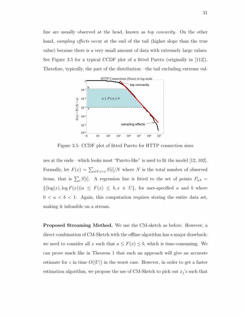
31
line are usually observed at the head, known as top concavity. On the other
hand, sampling effects occur at the end of the tail (higher slope than the true
value) because there is a very small amount of data with extremely large values.
See Figure 3.5 for a typical CCDF plot of a fitted Pareto (originally in [112]).
Therefore, typically, the part of the distribution—the tail excluding extreme val-
0 10 102 103 104 105 106 10710-6
10-5
10-4
10-3
10-2
10-1
1HTTP Connections (Sizes) in log-scale
x
F(x
) =
Pr
(X >
x)
a
b
( )a F x b
sampling effects
top concavity
Figure 3.5: CCDF plot of fitted Pareto for HTTP connection sizes
ues at the ends—which looks most “Pareto-like” is used to fit the model [12, 102].
Formally, let F (x) =∑
i∈U,i>x S[i]/N where N is the total number of observed
items, that is∑
i S[i]. A regression line is fitted to the set of points Pa,b =
{(log(x), log F (x))|a ≤ F (x) ≤ b, x ∈ U}, for user-specified a and b where
0 < a < b < 1. Again, this computation requires storing the entire data set,
making it infeasible on a stream.
Proposed Streaming Method. We use the CM-sketch as before. However, a
direct combination of CM-Sketch with the offline algorithm has a major drawback:
we need to consider all x such that a ≤ F (x) ≤ b, which is time-consuming. We
can prove much like in Theorem 1 that such an approach will give an accurate
estimate for z in time O(|U |) in the worst case. However, in order to get a faster
estimation algorithm, we propose the use of CM-Sketch to pick out xj ’s such that

32
xj ’s are approximate φ-quantiles, 0 < φ < 1, and a ≤ F (xj) ≤ b. Using CM-
Sketch, we get xj and the approximate value of F (xj), denoted F (xj). Let P be
the set of all (log xj , log F (xj)) such pairs. We will find the least squares fit to
these pairs and take its slope as the estimate −z. We can present an estimate for
the accuracy for this method by comparing against an offline algorithm. Suppose
z is obtained by plotting the set of points Q that is the set of all (log xj , log F (xj))
pairs, because F (xj)’s can be determined offline exactly. The slope of the best-fit
line gives −z for the Pareto parameter.
Theorem 4 Our algorithm uses O( log2 |U |ǫa
log log |U |δφ
) space, O(log log |U |δφ
log |U |)per-item processing time, and with probability at least 1 − δ, outputs estimate
z for z in O( log |U |φ
log log |U |δφ
) time such that:
|z − z| ≤ 2ǫ/(1− ǫ).
Proof. With O( log2 |U |ǫ′
log log |U |δ′
) space and per-item update time of O(log log |U |δ′
log |U |),
CM Sketch returns (xj , F (xj)) such that with probability at least 1− δ′, F (xj)−ǫ′ ≤ F (xj) ≤ F (xj) + ǫ′. Note that ∀xj , F (xj) ≥ a, so
(1− ǫ′/a)F (xj) = F (xj)− ǫ′F (xj)/a ≤ F (xj)
≤ F (xj) + ǫ′F (xj)/a
= (1 + ǫ′/a)F (xj).
Set ǫ′ = ǫa, then (1− ǫ)F (xj) ≤ F (xj) ≤ (1 + ǫ)F (xj). Therefore, our defined set
of points Q and P , from which z and z are computed by the slope of regression
lines, correspond to respective point set F and F defined before Theorem 1. The
rest of the proof of accuracy is similar to the proof of Theorem 1, and the time
and space bounds follow by replacing ǫ′ and δ′ with ǫa and δφ, respectively. The
time to output z is the time to find O(1/φ) quantiles.
33
3.4.3 Model Validation
Fractal model validation (see Section 3.3.3) relies on q-q plots, where the corre-
lation coefficient (cc) is used as a heuristic to measure the goodness-of-fit. The
Pareto model has infinite variance [112] and hence, the cc-based q-q test fails
directly because correlation is not even defined unless variances are finite. As
a result, both numerator and denomenator of the cc-formula are dominated by
extremely large values, leading the ratio to 1 regardless of whether the corre-
sponding z estimate is close to its true value or not. Therefore, we use q-q plot as
a visual construct to evaluate the goodness-of-fit. The basic building blocks of a
q-q plot are quantiles of real and generated data sets. Quantiles of real data can
be approximated accurately and efficiently by using the CM-Sketch, as before.
Online Quantile Generation. Finding quantiles of generated data without
materializng the entire data set is again a challenge. Luckily, the Pareto model
has well-defined CCDF Pr(X > x) = (c/x)z, where c = [z∑
x∈U x−(z+1)]−1/z . We
can derive that its i-th φ-quantile xi = c(iφ)−1/z. We do not know c even though
we have the model parameter z. However, any c will do since the expression for
φ-quantile says that the quantiles are linearly related under different c’s. Hence, if
quantiles of generated data are computed via any choice of c-value, the resulting
q-q plot should still be a straight line, though its slope is not necessarily 1. Since
the focus of our testing hypothesis is to validate the correctness of z, rather than
c, we use some arbitrary c to generate online q-q plot, to test goodness-of-fit of
the model, by comparing the generated plot against a straight line. Hence,
Theorem 5 Our algorithm uses O(1/φ) time and space to generate approximate
φ-quantiles directly from the Pareto model without materializing data.
Proof. First, select some c-value. Then the i-th φ-quantile xi = c(iφ)−1/z is
computed in O(1) time and space. There are at most 1/φ φ-quantiles to generate
34
from the region [a, b] of interest.
3.5 Fractal Model Fitting Experiments
In this section we evaluate the accuracy and performance of our proposed stream-
ing methods for fitting a b-model (see Section 3.3) against alternative methods.
Also, we implemented our method in AT&T’s Gigascope data stream manage-
ment system to demonstrate its practicality on a live data stream and examine
the robustness and stability of b-model fitting on several weeks of operational
data in an IP network. Finally, we study an intrusion detection application using
the b-model on traffic data labeled with known attacks.
3.5.1 Alternative Streaming Methods
We consider two alternative methods for estimating b: one based on Maximum
Likelihood Estimation (MLE), a common approach to model fitting in statis-
tics; and a straightforward heuristic which we dub pyramid approximation. We
will later compare these against our proposed method from Section 3.3, both in
concept and in practical performance.
Method 1: Maximum Likelihood Estimation.
Maximum likelihood estimation (MLE) of the parameter b involves finding
the value that maximizes the a posteriori likelihood of occurrence based on the
existing data. MLE is a time-honored technique described in many classical
statistics textbooks. Consider a single stage of the cascade construction with N
items observed in the parent interval, N1 in the heavier subinterval weighted b, and
N−N1 in the other. The probability of observing such an item distribution given
b is bN1(1− b)N−N1 . We can use this for multiple levels to derive formulas for b.
Define event A = {number of items observed at U(k)i = M
(k)i , ∀i ∈ {0, . . . , 2k−1}},
where M(k)i is the ith k-aggregate in U
(k)i at level k. Define M to be the total item

35
count, and B(k) = {i | U (k)i is assigned b fraction of the parent (p− 1)-aggregate
and i ∈ {0, . . . , 2k − 1}}. Then the likelihood function is
Lp(b|data) = Pr[A|data] =
p∏
k=1
∏
i∈B(k)
bM(k)i (1− b)
M(k−1)⌊i/2⌋
−M(k)i
= bPp
k=1
P
i∈B(k) M(k)i (1− b)pM−
Ppk=1
P
i∈B(k) M(k)i .
The log-likelihood function is
log Lp(b|data) = (
p∑
k=1
∑
i∈B(k)
M(k)i ) log b + (pM −
p∑
k=1
∑
i∈B(k)
M(k)i ) log(1− b).
Setting the derivative with respect to b to zero, we have bMLE =(Pp
k=1
P
i∈B(k) M(k)i )
pM.
Since |B(k)| = 2k−1, the overall running time is O(∑p
k=1 2k−1) = O(2p).
In summary, it takes O(2p) time to compute
bMLE = (
p∑
k=1
∑
i∈B(k)
M(k)i )/pM,
where M is the total item count, M(k)i is the ith k-aggregate in U
(k)i at level k,
and B(k) = {i | U(k)i is assigned b fraction of the parent (p − 1)-aggregate and
i ∈ {0, . . . , 2k − 1}}.
Example. For data in Figure 3.6, M = 5, when p = 2, B(1) = {0}, B(2) = {1, 2},bMLE = 3+(2+2)
2∗5= 0.7.
Since we cannot maintain all levels p on the data stream since 2p will exceed
available memory for large p, we use only the top few levels and thus the resulting
estimation error can be large.
Method 2: Pyramid Approximation.
This heuristic for estimating the parameter b is inspired by the so-called
“method of moments” from statistics, and immediately follows from the defi-
nition of the b-model. It aggregates the data at multiple prefix levels and then
independently finds the best fit to the fractions, at each level, based on the cor-
responding prefix aggregates; see Figure 3.6 for an illustration.
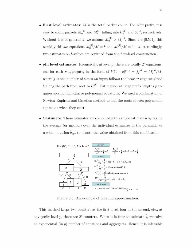
36
• First level estimates: M is the total packet count. For 1-bit prefix, it is
easy to count packets M(1)0 and M
(1)1 falling into U
(1)0 and U
(1)1 , respectively.
Without loss of generality, we assume M(1)0 > M
(1)1 . Since b ∈ [0.5, 1], this
would yield two equations M(1)0 /M = b and M
(1)1 /M = 1− b. Accordingly,
two estimates on b-values are returned from the first-level construction.
• pth level estimates: Recursively, at level p, there are totally 2p equations,
one for each p-aggregate, in the form of bj(1 − b)p−j = f(p)i = M
(p)i /M ,
where j is the number of times an input follows the heavier edge weighted
b along the path from root to U(p)i . Estimation at large prefix lengths p re-
quires solving high-degree polynomial equations. We used a combination of
Newton-Raphson and bisection method to find the roots of such polynomial
equations when they exist.
• b estimate: These estimates are combined into a single estimate b by taking
the average (or median) over the individual estimates in the pyramid; we
use the notation bpyr to denote the value obtained from this combination.
b
b
5*
1*
1-b
b1-b
23
0
11
2
00 01 10
12
0*1-b
U = {00, 01, 10, 11}, M = 5Level 1
Level 2
(1)0 3
;5
Mb
M
(1)1 2 3
15 5
Mb b
M
(2)
01
(1 ) 0.7236;5
M
Mb b b
(2)21
20.6325;
5M
Mb b
(2)
22(1 )
5M
Mb b no root;
(2)23
0(1 ) 1.
5M
Mb b
b estimate
(0.6 0.6 0.7236 0.6325 1)0.71122
5.b
Figure 3.6: An example of pyramid approximation.
This method keeps two counters at the first level, four at the second, etc.; at
any prefix level p, there are 2p counters. When it is time to estimate b, we solve
an exponential (in p) number of equations and aggregates. Hence, it is infeasible

37
both to store this many counters and to solve as many polynomial equations for
all levels of the pyramid. In the streaming setting, we will therefore use this
method only for the top few levels (say p = O(log log |U |)). This does not provide
any guaranteed error for b estimation.
3.5.2 Accuracy of Proposed Method
Parameter Estimation. For control purposes, we generated synthetic data
using the stack-based algorithm in [110]. Given a bias b, data volume N , and
number of levels k, this random generator returns (val, freq) pairs. In our case,
we set N to 108 and k to 32 (to simulate the IPv4 domain); b ranged between 0.55
and 0.95. We evaluated the offline method for deriving an estimate of b on the
data sets to isolate out additional error resulting from sketches that are needed
for online estimation, so that the effectiveness of the offline algorithm in deriving
a correct estimate of b, based on correlation dimension, is evaluated. We see in
Table 3.1 that b2 is almost identical to b.
b b2 b b2 b b2
0.55 0.62 0.70 0.7009 0.85 0.8500000.60 0.63 0.75 0.75007 0.90 0.9000000.65 0.66 0.80 0.800002 0.95 0.950000
Table 3.1: Estimates of b on synthetically generated data.
We observed that the difference between b and b2 becomes smaller as b in-
creases. Recall that the distribution becomes more biased with increasing b. For
less biased data, if the data size is less than |U |, truncation errors of bucket counts
affect the accuracy of b2.
We repeated this experiment, using the same methods, on IP addresses from
real TCP packets in the AT&T network collected from a full hour and repeated
the measurements over the course of multiple consecutive hours to examine the
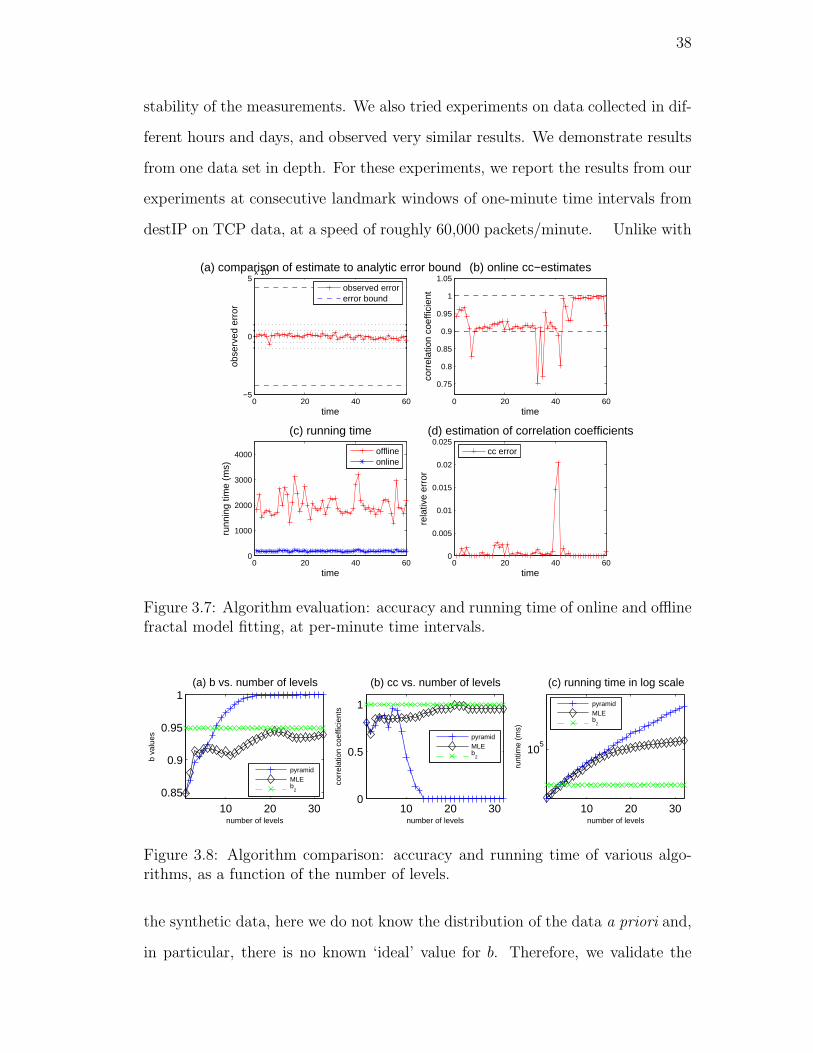
38
stability of the measurements. We also tried experiments on data collected in dif-
ferent hours and days, and observed very similar results. We demonstrate results
from one data set in depth. For these experiments, we report the results from our
experiments at consecutive landmark windows of one-minute time intervals from
destIP on TCP data, at a speed of roughly 60,000 packets/minute. Unlike with
0 20 40 60−5
0
5x 10
−3
time
obse
rved
err
or
(a) comparison of estimate to analytic error bound
observed errorerror bound
0 20 40 60
0.75
0.8
0.85
0.9
0.95
1
1.05
time
corr
elat
ion
coef
ficie
nt
(b) online cc−estimates
0 20 40 600
1000
2000
3000
4000
time
runn
ing
time
(ms)
(c) running time
offlineonline
0 20 40 600
0.005
0.01
0.015
0.02
0.025
time
rela
tive
erro
r(d) estimation of correlation coefficients
cc error
Figure 3.7: Algorithm evaluation: accuracy and running time of online and offlinefractal model fitting, at per-minute time intervals.
10 20 300.85
0.9
0.95
1
number of levels
b va
lues
(a) b vs. number of levels
pyramidMLEb
2
10 20 300
0.5
1
number of levels
corr
elat
ion
coef
ficie
nts
(b) cc vs. number of levels
pyramidMLEb
2
10 20 30
105
number of levels
runt
ime
(ms)
(c) running time in log scale
pyramidMLEb
2
Figure 3.8: Algorithm comparison: accuracy and running time of various algo-rithms, as a function of the number of levels.
the synthetic data, here we do not know the distribution of the data a priori and,
in particular, there is no known ‘ideal’ value for b. Therefore, we validate the
39
goodness-of-fit using the correlation coefficient, denoted cc, obtained from quan-
tiles of the data compared to those from data that would be generated by the
model (known as the q-q test and described in Section 3.3). In all experiments,
we first consider the approximation error resulting from the underlying CM (the
sketch width was 512 units) technique by comparing the offline D2 estimates with
its online counterparts. As we showed in Section 3.3.2, the error of the approach
based on D2 is bounded (with high probability). Indeed, this bound tends to hold
in practice; see Figure 3.7(a). A similar trend occurs with the differences between
online and offline estimates for b2, since they can be derived from D2, but we
are presenting the error with respective to D2 here because the error bounds are
independent of D2 and thus more intuitive to present graphically. We also plot
the q-q test correlation coefficients from b-value estimates based on the online
approaches as shown in Figure 3.7(b). Here the correlation coefficient for b2 is
close to 1 at almost all time intervals, indicating a good model fitting. Moreover,
running time of the online algorithm, measured by Unix time command, shown in
Figure 3.7(c), is at least an order of magnitude faster than its offline counterpart.
Online Goodness-of-Fit Estimates. The correlation coefficients used to evalu-
ate the goodness-of-fit of b in the experiments above were computed offline because
the q-q tests require quantiles from the data stream as well as from data gener-
ated from the fractal model using b. How accurate are the correlation coefficient
estimates for our proposed method using approximate quantiles in comparison to
those computed offline (using exact quantiles)? Figure 3.7(d) indicates that the
difference is insignificant, in most cases within an absolute difference of 0.0025,
and in the (rare) worst case within 0.017.
3.5.3 Comparison of Methods
We have three methods for estimating b on a data stream. The pyramid and MLE
methods only explore the top few levels since the space used by them explodes

40
exponentially as the levels are increased. In contrast, our proposed method from
Section 3.2 uses small space per level and hence is able to explore the entire depth
of the hierarchy. Furthermore, the proposed method provides accuracy guarantees
on b.
We compared these three methods on IP addresses from TCP packet traf-
fic data. We varied the number of levels (from 1 to 32) used to derive b, but
found that for pyramid approximation, this marginally improved the estimates
at medium levels, and deteriorated the accuracy with too many levels; for MLE,
bMLE gradually converged to b2 with many levels considered. Figure 3.8(a)(b)
summarize the results. For comparison, the estimates for b2 are plotted as a
straight line. Here pyramid approximation yielded the worst estimates. As shown
in Figure 3.8(b), the correlation coefficient for b2 is always higher than that based
on pyramid approximation at any level. Pyramid method has many sources of
error: approximation error from the numerical solution of high-degree polynomi-
als, sometimes such polynomials do not have roots, limiting the number of levels
to fit the space constraints, etc. In contrast, MLE is more robust. bMLE starts
behaving well after level 21, with stable goodness-of-fit measures thereafter. Fig-
ure 3.8(c) summarizes the running time to estimate bpyr, bMLE and b2 in the log
scale as a function of the number of levels. The limitations of pyramid and MLE
methods are apparent; hence, we do not consider them in the remainder of our
experiments.
3.5.4 Performance On a Live Data Stream
We implemented the proposed method, based on estimating D2 using CM sketches,
as a User-Defined Aggregate Function (UDAF) facility in Gigascope [29], a highly
optimized system for monitoring very high speed data streams [37]. The source
used for these performance experiments was a live IP packet stream monitored
at a network interface inside the AT&T network, and the whole experiment ran
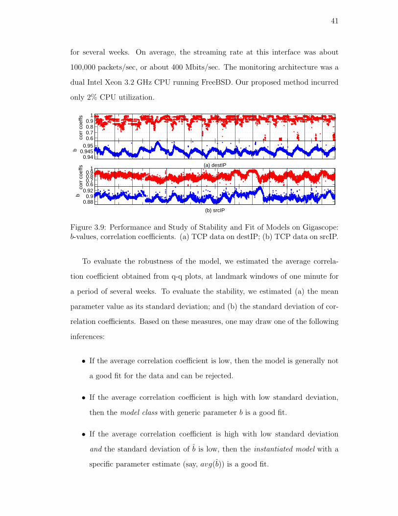
41
for several weeks. On average, the streaming rate at this interface was about
100,000 packets/sec, or about 400 Mbits/sec. The monitoring architecture was a
dual Intel Xeon 3.2 GHz CPU running FreeBSD. Our proposed method incurred
only 2% CPU utilization.
0.60.70.80.9
1
corr
coe
ffs
0.880.9
0.92
b
(b) srcIP
0.60.70.80.9
1
corr
coe
ffs
0.940.945
0.95
b
(a) destIP
Figure 3.9: Performance and Study of Stability and Fit of Models on Gigascope:b-values, correlation coefficients. (a) TCP data on destIP; (b) TCP data on srcIP.
To evaluate the robustness of the model, we estimated the average correla-
tion coefficient obtained from q-q plots, at landmark windows of one minute for
a period of several weeks. To evaluate the stability, we estimated (a) the mean
parameter value as its standard deviation; and (b) the standard deviation of cor-
relation coefficients. Based on these measures, one may draw one of the following
inferences:
• If the average correlation coefficient is low, then the model is generally not
a good fit for the data and can be rejected.
• If the average correlation coefficient is high with low standard deviation,
then the model class with generic parameter b is a good fit.
• If the average correlation coefficient is high with low standard deviation
and the standard deviation of b is low, then the instantiated model with a
specific parameter estimate (say, avg(b)) is a good fit.

42
We estimated b2 and its corresponding correlation coefficient cc on multiple
simultaneous groupings of the data (on either srcIP or destIP addresses, and for
either TCP, UDP, ICMP, or all IP packets). Figure 3.9 illustrates the time series
of b2 and cc for (a) destIP and (b) srcIP on TCP data, for a period of several
weeks.
Figure 3.9(a) shows a fairly robust fit for the instantiated model, with mean
correlation coefficient 0.918 and standard deviation 0.0662. In addition, the es-
timate for b was quite stable, fluctuating within a very small range [0.928, 0.985]
with mean value 0.945 and standard deviation 0.002 over the interval of several
weeks. Some additional observations:
• The cc values were highest when b2 was near the mean value and lowest the
further b2 was from the mean in either direction.
• Such fluctuations occurred at regular cycles.
• The fluctuations of cc appear to correlate with the traffic distribution (de-
scribed by b2).
• The time series was generally ‘smooth’, that is, the change in value of b
at consecutive time steps was usually very small. However, there were
occasional instances of large jumps, perhaps indicating outliers in the data.
As a ‘sanity check’, we tried to skew the distribution on srcIP addresses by
selecting only packets originating from three different ISPs. The resulting tri-
modal distribution should therefore not be suitable for our model. As expected,
the average cc in Figure 3.9(b) is 0.7612, and dips below 0.5 for some windows.
Accordingly, b2 has a standard deviation of .011, which is an order of magnitude
higher than that on destIP.
The results on UDP and ICMP packets indicate that the fractal model does
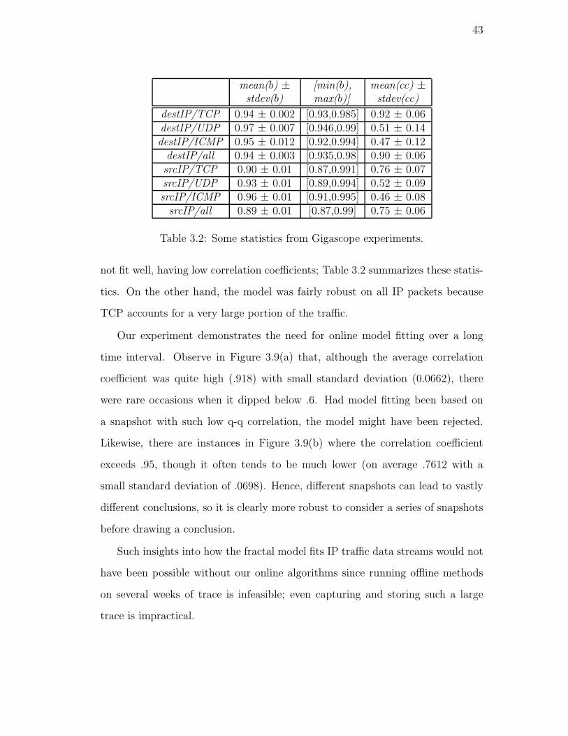
43
mean(b) ± [min(b), mean(cc) ±stdev(b) max(b)] stdev(cc)
destIP/TCP 0.94 ± 0.002 [0.93,0.985] 0.92 ± 0.06destIP/UDP 0.97 ± 0.007 [0.946,0.99] 0.51 ± 0.14destIP/ICMP 0.95 ± 0.012 [0.92,0.994] 0.47 ± 0.12
destIP/all 0.94 ± 0.003 [0.935,0.98] 0.90 ± 0.06srcIP/TCP 0.90 ± 0.01 [0.87,0.991] 0.76 ± 0.07srcIP/UDP 0.93 ± 0.01 [0.89,0.994] 0.52 ± 0.09srcIP/ICMP 0.96 ± 0.01 [0.91,0.995] 0.46 ± 0.08
srcIP/all 0.89 ± 0.01 [0.87,0.99] 0.75 ± 0.06
Table 3.2: Some statistics from Gigascope experiments.
not fit well, having low correlation coefficients; Table 3.2 summarizes these statis-
tics. On the other hand, the model was fairly robust on all IP packets because
TCP accounts for a very large portion of the traffic.
Our experiment demonstrates the need for online model fitting over a long
time interval. Observe in Figure 3.9(a) that, although the average correlation
coefficient was quite high (.918) with small standard deviation (0.0662), there
were rare occasions when it dipped below .6. Had model fitting been based on
a snapshot with such low q-q correlation, the model might have been rejected.
Likewise, there are instances in Figure 3.9(b) where the correlation coefficient
exceeds .95, though it often tends to be much lower (on average .7612 with a
small standard deviation of .0698). Hence, different snapshots can lead to vastly
different conclusions, so it is clearly more robust to consider a series of snapshots
before drawing a conclusion.
Such insights into how the fractal model fits IP traffic data streams would not
have been possible without our online algorithms since running offline methods
on several weeks of trace is infeasible; even capturing and storing such a large
trace is impractical.
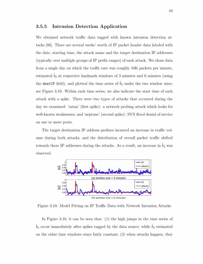
44
3.5.5 Intrusion Detection Application
We obtained network traffic data tagged with known intrusion detection at-
tacks [86]. There are several weeks’ worth of IP packet header data labeled with
the date, starting time, the attack name and the target destination IP addresses
(typically over multiple groups of IP prefix ranges) of each attack. We chose data
from a single day on which the traffic rate was roughly 10K packets per minute,
estimated b2 at respective landmark windows of 3 minutes and 6 minutes (using
the destIP field), and plotted the time series of b2 under the two window sizes;
see Figure 3.10. Within each time series, we also indicate the start time of each
attack with a spike. There were two types of attacks that occurred during the
day we examined: ‘satan’ (first spike): a network probing attack which looks for
well-known weaknesses; and ‘neptune’ (second spike): SYN flood denial of service
on one or more ports.
The target destination IP address prefixes incurred an increase in traffic vol-
ume during both attacks, and the distribution of overall packet traffic shifted
towards these IP addresses during the attacks. As a result, an increase in b2 was
observed.
0.96
0.97
0.98
0.99
1
b2
(b) window size = 6 minutes
b2
attacks
0.960.970.980.99
1
b2
(a) window size = 3 minutes
b2
attacks
Figure 3.10: Model Fitting on IP Traffic Data with Network Intrusion Attacks
In Figure 3.10, it can be seen that: (1) the high jumps in the time series of
b2 occur immediately after spikes tagged by the data source, while b2 estimated
on the other time windows stays fairly constant; (2) when attacks happen, they

45
usually last for awhile, resulting in b2 staying high, in contrast to the small fluctu-
ations during other intervals; and (3) at the larger window size (Figure 3.10(b)),
the time series of b2 flattens out while the network is not being attacked whereas
the b-values estimated during attacks remain high.
Given the fact that, under normal traffic conditions, mean(b2) = 0.962, stdev(b2) =
0.007, an increase in b2 to above 0.985 is a potential indicator of anomalies in this
time series. This suggests that fitting the b-model parameter online has potential
“discriminatory power” for intrusion detection monitoring. Still, flexible stream-
ing algorithms like ours are needed to get a good understanding of the variability
of b2 and cc over time to infer critical things about IP network traffic distribution.
3.6 Pareto Model Fitting Experiments
3.6.1 Alternative Streaming Method
We again consider the maximum likelihood estimator of tail index z. Suppose we
have N observed item values (e.g. flow sizes), x1, . . . , xN . For the Pareto model,
Pr(X > x) = (c/x)z where c is the scaling constant. So Pr(X = x) = czzx−(z+1).
Given the observed sequence, its log-likelihood function is
l(x1, . . . xN |z) = Nz log c + N log z − (z + 1)∑N
i=1 log xi.
Setting its derivative with respect to z to zero, we get
zMLE =N(1 + log c)∑N
i=1 log xi
.
The denominator can be computed exactly on the fly. But the difficulty is com-
puting c. In theory, c satisfies∑
x∈U Pr(X = x) =∑
x∈U czzx−(z+1) = 1 since the
distribution is a probability function. Hence, c = [z∑
x∈U x−(z+1)]−1/z; and zMLE
is derived by solving the equation z =N [1−(log(z
P
x∈U x−(z+1)))/z]PN
i=1 log xifor z. Although
it is theoretically feasible to exploit numerical techniques to find its root, it is
practically infeasible in the streaming case since the number of log-terms in the

46
numerator is linearly proportional to the domain size which is prohibitive. So,
as an alternative, we adapt the commonly-used heuristic of setting c = xmin, the
minimum x-value [5], so that Pr(X > xmin) = 1, which satisfies the definition of a
probability function, and present experimental study exploring this choice of c.
3.6.2 Accuracy of Proposed Method
In all experiments, the range of the distribution that is of interest is, by default,
a = 1% ≤ F (x) ≤ 15% = b.
Synthetic data. For control purposes, We used a standard simulation tech-
nique, the so-called inverse transformation method, to generate values from a
Pareto distribution with specified tail index z. Each experiment consisted of
drawing N = 108 items from a domain of size |U | = 107. We ran our proposed
method to recover z from the entire tail [a, b] of the generated data sets. Table 3.3
shows that z-estimates are more accurate for z in (0.2, 1.8) than at the extremes.
The difference between z and z becomes smaller as |U | or N increases.
z z z z z z
0.2 0.477 0.8 0.8002 1.4 1.3660.4 0.428 1.0 0.9991 1.6 1.4960.6 0.6009 1.2 1.1996 1.8 1.638
Table 3.3: Estimates of z on synthetically generated data.
Flow Data. We compared the proposed streaming method with the existing
offline one on flow sizes (in terms of number of bytes per flow) using NetFlow
data collected at a router over multiple consecutive hours. We selected out all
sessions for which the number of packets per flow is greater than 3 to exclude
TCP SYN attacks. Similar results were observed from data collected in different
hours, so we reported our experimental results from one-hour data set in depth, at
consecutive landmark windows of two-minute time intervals, consisting of 100K
flows on average.
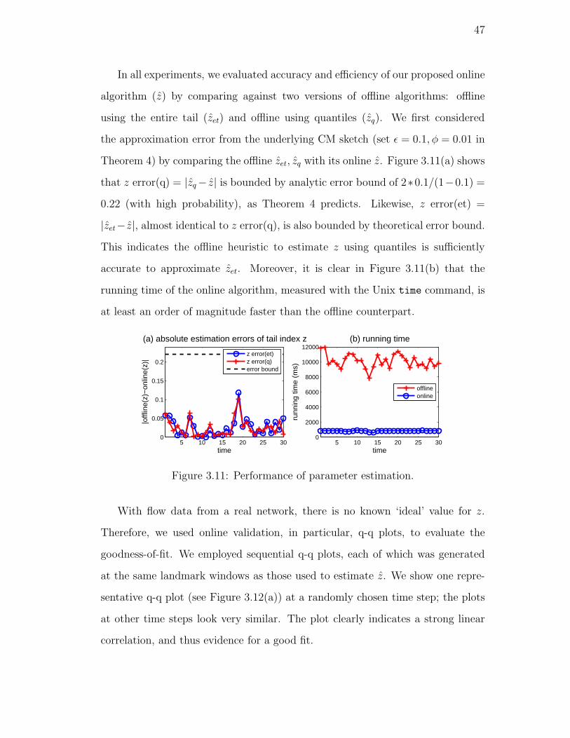
47
In all experiments, we evaluated accuracy and efficiency of our proposed online
algorithm (z) by comparing against two versions of offline algorithms: offline
using the entire tail (zet) and offline using quantiles (zq). We first considered
the approximation error from the underlying CM sketch (set ǫ = 0.1, φ = 0.01 in
Theorem 4) by comparing the offline zet, zq with its online z. Figure 3.11(a) shows
that z error(q) = |zq− z| is bounded by analytic error bound of 2∗0.1/(1−0.1) =
0.22 (with high probability), as Theorem 4 predicts. Likewise, z error(et) =
|zet− z|, almost identical to z error(q), is also bounded by theoretical error bound.
This indicates the offline heuristic to estimate z using quantiles is sufficiently
accurate to approximate zet. Moreover, it is clear in Figure 3.11(b) that the
running time of the online algorithm, measured with the Unix time command, is
at least an order of magnitude faster than the offline counterpart.
5 10 15 20 25 300
0.05
0.1
0.15
0.2
time
|offl
ine(
z)−
onlin
e(z)
|
(a) absolute estimation errors of tail index z
z error(et)z error(q)error bound
5 10 15 20 25 300
2000
4000
6000
8000
10000
12000
time
runn
ing
time
(ms)
(b) running time
offlineonline
Figure 3.11: Performance of parameter estimation.
With flow data from a real network, there is no known ‘ideal’ value for z.
Therefore, we used online validation, in particular, q-q plots, to evaluate the
goodness-of-fit. We employed sequential q-q plots, each of which was generated
at the same landmark windows as those used to estimate z. We show one repre-
sentative q-q plot (see Figure 3.12(a)) at a randomly chosen time step; the plots
at other time steps look very similar. The plot clearly indicates a strong linear
correlation, and thus evidence for a good fit.

48
3.6.3 Comparison of Methods
We repeated our experiments on flow data by comparing our proposed online
method (z) with MLE. As we mentioned earlier, one problem with MLE is finding
the best scaling constant c, from which zMLE is derived. We demonstrate the
ad-hocness of picking a c for the MLE estimator by computing zMLE based on
three different c-values: minimum observed x-value, its minimum domain value,
the average of the above two minimums, all of which satisfy the definition of a
probability function (i.e. Pr(X > c) = 1). We denote the respective zMLE as
zmo, zmd, zma. The average z-values, computed via different methods over all time
steps, are listed below:
z zmo zmd zma
1.37 0.78 0.19 0.68
0 2 4 6 8 10
x 104
0
1000
2000
3000
4000
5000
6000
7000
real data
gene
rate
d da
ta
(a) q−q plot
line−fitting
0 2 4 6 8
x 104
0
2
4
6
8x 10
4
real data
gene
rate
d da
ta
(b) q−q plot
MLE−mo
0 2 4 6 8
x 104
0
0.5
1
1.5
2
2.5
3x 10
13
real data
gene
rate
d da
ta
(c) q−q plot
MLE−md
0 2 4 6 8
x 104
0
0.5
1
1.5
2x 10
5
real data
gene
rate
d da
ta
(d) q−q plot
MLE−ma
Figure 3.12: Algorithm comparison.
Note the wide disparity in z estimates between the proposed method and MLE-
based approaches. We now examine their goodness-of-fits. The q-q plot for the

49
proposed method (Figure 3.12(a)) is clearly more linear compared to the other
methods (Figures 3.12(b)-(d)) .
In addition, the above list of z estimates also tells us that zMLE in general
under-estimates z because of the top concavity.
3.7 Extensions
Other Streaming Windows. On the stream, our methods need to simply
maintain aggregates such as L2 norms, range sums and quantiles. We used the
CM-Sketch for this purpose with the landmark window model. Our methods
directly generalize to other streaming models. For example, in presence of inserts
and deletes, the CM-Sketch methods dynamically maintain all these aggregates
with equal accuracy as when only inserts are allowed. Similarly, with a windowed
stream model, these aggregates can be maintained accurately using [40, 8]. Also,
in the model where the past is continuously weighted down as the stream comes
in, there are similar results for maintaining our desired aggregates [27]. Therefore,
in all these variations of streaming windows, our methods work and give similar
guarantees as the ones we show here with landmark windows. Our contribution
is not in designing the synopses structures for different window models, but in
showing how to use them for parameter estimation and validation, and proving
accuracy guarantees in the process.
Fitting Other Models.
Hausdorff Fractal Dimension D0. Recall notations used to define fractal
model in Section 3.3.1. Set V = {0 . . . , log |U |}. Hausdorff fractal dimension D0
is defined when
N(p) =
2p−1∑
i=0
1(P(i+1)2log |U|−p−1
j=i2log |U|−pS[j]>0)
, ∀p ∈ V,
and 1() is an indicator function. Instead of using the CM sketch to estimate
log N(p) to derive D2, we use hierarchical Flajolet-Martin, or FM, sketch [51] to
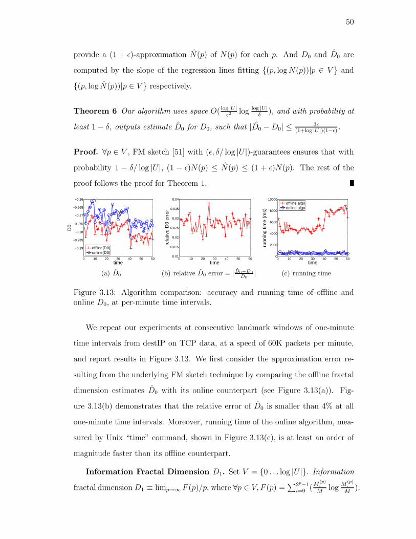
50
provide a (1 + ǫ)-approximation N(p) of N(p) for each p. And D0 and D0 are
computed by the slope of the regression lines fitting {(p, log N(p))|p ∈ V } and
{(p, log N(p))|p ∈ V } respectively.
Theorem 6 Our algorithm uses space O( log |U |ǫ2
log log |U |δ
), and with probability at
least 1− δ, outputs estimate D0 for D0, such that |D0 −D0| ≤ 3ǫ(1+log |U |)(1−ǫ)
.
Proof. ∀p ∈ V , FM sketch [51] with (ǫ, δ/ log |U |)-guarantees ensures that with
probability 1 − δ/ log |U |, (1 − ǫ)N(p) ≤ N(p) ≤ (1 + ǫ)N(p). The rest of the
proof follows the proof for Theorem 1.
0 10 20 30 40 50 60
−0.29
−0.285
−0.28
−0.275
−0.27
−0.265
−0.26
time
D0
offline(D0)online(D0)
(a) D0
0 10 20 30 40 50 600.01
0.015
0.02
0.025
0.03
0.035
0.04
time
rela
tive
D0
erro
r
(b) relative D0 error = | D0−D0
D0
|
0 10 20 30 40 50 600
2000
4000
6000
8000
10000
timeru
nnin
g tim
e (m
s)
offline algoonline algo
(c) running time
Figure 3.13: Algorithm comparison: accuracy and running time of offline andonline D0, at per-minute time intervals.
We repeat our experiments at consecutive landmark windows of one-minute
time intervals from destIP on TCP data, at a speed of 60K packets per minute,
and report results in Figure 3.13. We first consider the approximation error re-
sulting from the underlying FM sketch technique by comparing the offline fractal
dimension estimates D0 with its online counterpart (see Figure 3.13(a)). Fig-
ure 3.13(b) demonstrates that the relative error of D0 is smaller than 4% at all
one-minute time intervals. Moreover, running time of the online algorithm, mea-
sured by Unix “time” command, shown in Figure 3.13(c), is at least an order of
magnitude faster than its offline counterpart.
Information Fractal Dimension D1. Set V = {0 . . . log |U |}. Information
fractal dimension D1 ≡ limp→∞ F (p)/p, where ∀p ∈ V, F (p) =∑2p−1
i=0 (M
(p)i
Mlog
M(p)i
M).

51
Using appropriate sketches to estimate the entropy [21, 66, 20] hierarchically, we
can obtain strong accuracy estimates for calculating the information fractal di-
mension as well.
Our overall approach here of (a) rigorous analysis of fitting regression line to
various plots that are populated with estimations from synopses maintained over
the data streams and (b) online validation using q-q plots that work without ma-
terializing the generated data, is powerful and will find many other applications.
3.8 Related Work
Parametric model fitting has a long history in the statistics literature, where the
goal is to find parameter value(s) which best match the observed data. Many dif-
ferent methods have been proposed, from the “method of moments” to maximum
likelihood estimators. There are trade-offs for different distributions to which
they are applied. Our challenge here is to adapt the commonly used model fitting
methods for skewed data to the streaming scenario.
There has been plethora of methods for managing data streams in general [96].
They have primarily focused on clustering (k-means or k-medians), summarizing
(quantiles or histograms or wavelets) or mining (heavy hitters, change detection).
In contrast to the bulk of this literature, our focus is on modeling of data streams
using parametric models.
A number of different observations have been made about IP network traffic.
For example, IP traffic tends to have bursty behavior [81]; it tends to have heavy-
tailed distributions [112] and exhibit self-similarity in multiple scales [61]. There
is a hierarchical component to their distribution over the IP address space that
resonates with the hierarchical assignment of IP addresses to domains [26]. On
the other hand, non-hierarchical skew of many real data sources is observed and
well modeled by heavy-tailed—in particular, Pareto—distributions [112]. One
52
needs suitable models (hierarchical and non-hierarchical), preferably with a small
number of parameters, to describe the inherent characteristics of IP traffic [114].
Regarding hierarchical model fitting, the most relevant work is [81], where they
identified IP traffic streams as having the fractal behavior (using offline methods)
and demonstrated that the fractal dimension of traffic over the IP address hier-
archy can serve as a “fingerprint” for traffic at different sites and times. From an
algorithmic perspective, a highly relevant work is [110], where the authors studied
the b-model and showed how to estimate b. Their algorithm was focused on tem-
poral modeling of IO systems and does not work on IP traffic streams because it
requires that values arrive in sorted order. Another related algorithmic result is
by [115], where they used the tug-of-war sketch to estimate the fractal dimension.
However, their approach does not provide error guarantees, which is our crucial
focus, and requires more space and update time than ours. Likewise, a lot of
work exists for (offline) fitting of Pareto models [12, 102, 114, 112]. However, we
are not aware of any prior work that exists on fitting Pareto distributions in data
streams.
We build on the existing literature in two key ways. First, all our methods are
streaming, that is, work online within small space and provide the first provable
online guarantees for the accuracy of parameter estimate(s); in contrast, existing
analyses are offline. Second, we introduce online validation of these parameter
estimates, which was not present in previous work and is crucially needed in the
data stream context where distributions and models change over time. Much of
our insights into real live IP streams in Sections 3.5.4 and 3.5.5 would have been
infeasible to get with the offline methods.

53
3.9 Chapter Summary
There has been a lot of work on techniques for analyzing streaming data, but very
little has focused on modeling the data. We presented a highly efficient approach
for (a) estimating paramaters of (non-) hierarchical models on streams such as
IP traffic with guaranteed accuracy, and (b) online model validation, all within
small space and fast update time per new data stream item.
Statistical modeling is a difficult task and it needs careful, systematic and
rigorous real life experimental study to be robust. We performed detailed study
of our methods on an operational DSMS (AT&T’s Gigascope). Fortunately, our
approach only relied on maintaining CM-Sketches on the data stream and this
was already part of Gigascope for other operational reasons; hence, our approach
does not add any additional burden on the system. Also, we benefited from a
number of optimizations in Gigascope for this primitive. As a result, our detailed
study of modeling on several weeks of IP traffic streams reveals many insights on
its applicability and its use. In particular, our online validation approach proved
crucial and we believe it will be of fundamental interest in DSMSs for modeling
streams.

54
Algorithm 1 GeneratedQuantiles(cmh,b,φ) Stack-based method to gener-ate φ-quantiles Y directly from b-model
1: percent← 0 /*percentage of data generated*/2: addr ← 0 /*item ID*/3: i← 1 /*next quantile*/4: push a pair (1,0,0)5: while stack not empty do6: pop a tuple (frac, level, index) from the stack7: if level == log |U | then8: percent+ = frac9: while (percent >= iφ) and (i < 1/φ) do
10: Y [i] = addr; i + +11: end while12: addr + +13: else if percent + frac <= iφ then14: /* prune the subtree: no quantiles*/15: percent+ = frac; addr+ = 2log |U |−level
16: else17: /*assign weights according to range queries*/18: wl = CMH Count(cmh, level + 1, 2 ∗ index)19: wr = CMH Count(cmh, level + 1, 2 ∗ index + 1)20: if (wl < wr) then21: /*left (1-b), right b*/22: if percent + frac ∗ (1− b) < iφ then23: /*prune left branch: no quantiles*/24: percent+ = frac ∗ (1− b)25: addr+ = 2log |U |−level−1
26: /*push the right branch*/27: push (frac ∗ b,level + 1,2 ∗ index + 1)28: else29: push (frac ∗ b,level + 1,2 ∗ index + 1)30: push (frac ∗ (1− b),level + 1,2 ∗ index)31: end if32: else33: /*left b, right (1-b)*/ symmetric with L21-31, exchange b and 1−b34: end if35: end if36: end while37: return Y /*φ-quantiles*/

55
Chapter 4
Modeling Communication Graphs via Signatures
4.1 Introduction
In the everyday world, instances of interaction or communication between individ-
uals are everywhere. For example, individuals speak to each other via telephone;
IP traffic is passed between hosts; authors write documents together and so on.
There are other examples in which individuals interact with other entities, such as
when users pose search queries; post and comment on messages on bulletin boards
or blog sites; or when stock traders transact stocks, bonds and other goods. In
an indirect sense, users “communicate” with each other via the common objects.
In all cases the communication between individuals can be repeated many times
(such as in the case of telephone calls) and weighted (say, the quantity of stock
bought, or the duration of a call).
Given this abundance of communication between individuals, many applica-
tions rely on analyzing the patterns behind the communications, for example:
• Anti-Aliasing: is an individual behind multiple presences in the communica-
tion network? This happens e.g. when an individual has multiple connection
points (home, office, hotspot) to the Internet.
• Security: has some individual’s ‘identity’ been taken over by someone else?
This happens when a person is given access to another’s laptop, or when
a cellphone is stolen and used by someone else. Is a new user who arrives
at a particular time really the reappearance of an individual who has been

56
observed earlier? This happens in telephone networks when a consumer
defaults on an account and opens a fresh account to further use services
without paying (a “repetitive debtor”); or in bulletin boards when a banned
user re-registers with a new ID.
• Privacy Preservation: can we identify nodes from an anonymized graph
given outside information about known communication patterns per indi-
vidual? This happens in author identification of double-blind submissions.
Each of the questions above and others of this nature that rely on communi-
cation patterns can naturally be solved by designing suitable signatures for the
individuals. Informally, signatures capture the distinctive or discriminatory com-
munication behavior of an individual (telephone user, IP address, trader or user
of a search service, etc). While the concept of signatures is self-evident, formal-
izing and applying signatures to a specific task is really an art. Typically, in any
particular task, “signatures” are defined based on intuition and experimentally
validated against a labeled set. This approach has been instantiated successfully
for certain specific communication settings and applications. It was done for tele-
phone networks in [36, 68] where the authors defined a community of interest
to be the top-k numbers called by a given telephone number. With appropriate
age weighting and a suitable k, this was argued to be highly discriminatory for
detecting repetitive debtors. A second example is when a signature formed from
bibliographic citations is used to identify authors of double-blind submissions [69].
There are many other examples in areas including Security [83, 48, 35, 36], Net-
working [99, 117, 85, 98], Social Network Analysis [59, 15, 107], Epidemiology
and others.
In this chapter, we adopt the signature-based approach to analyzing the pat-
terns of communication exhibited by individuals. However, we focus on the pro-
cess of how signatures are developed and applied. In prior works, typically, one

57
considers a particular application, proposes an intuitive signature and evaluates
it empirically on datasets. We focus on principles behind the usage of signatures.
In particular, we propose the framework in which we first agree on a set of proper-
ties of signatures that are natural, and when faced with an application, determine
what properties of signatures are needed, and then, seek out examples of signa-
tures already known or design new ones which will have those properties. Hence,
the process will focus on abstract properties that are needed, and “shopping” for
signatures with those properties.
We develop a framework for the formal use of signatures for tasks that involve
analyzing communication patterns, for very general notions of communication.
We model the communications between entities using a suitably weighted graph,
and define a signature of a node abstractly in terms of the graph. Our contribu-
tions are:
• We identify basic properties of signatures such as persistence, uniqueness
and robustness, and for several tasks that involve analyzing communication
patterns, study which of these properties are needed. For example, a task
such as finding multiple presences of the same individuals in a time window
does not need signatures to be persistent; likewise, analyzing the changing
behavior of a single individual over time may not need signatures to be
discriminating.
• We consider specific signatures — some previously known, others new — for
communication graphs and study what basic properties they have, using ex-
tensive experiments with real datasets. This helps identify which signatures
are suitable for each of the tasks.
• We complement our conceptual results with a detailed experimental study
on two concrete applications of enterprise network traffic. We adopt the
framework for respective tasks. Our results show that signatures based on

58
a combination of a few application-desired properties is quite effective for
us.
It remains the case that finding suitable signatures for any task is more of an
art than a science, with effectiveness determined experimentally. In this sense,
our proposal of specific signatures for communication graphs and their application
to the specific tasks is such a study. But beyond this, our framework is general
and can be applied broadly.
In what follows, we first introduce our framework for analyzing signatures
in Section 4.2, the properties we desire, and an analysis of their values for a
variety of applications. In Section 4.3, we describe various signature schemes
based on expected features of communication graphs, and their characteristics.
We evaluate signatures empirically, first studying the general characteristics in
Section 4.4, and then for particular applications in Section 4.5. We lastly discuss
scalability issues in Section 4.6, then survey related work and give concluding
remarks.
4.2 Framework
Here we describe our framework for designing and evaluating topological signa-
tures for communication graphs. We define the domain of our signatures, and
three general properties for evaluating them. Finally, we discuss how these prop-
erties relate to specific applications of signatures.
4.2.1 Individuals and Labels
A communication graph is defined by the observed patterns of communications
between nodes representing individual users. However, we observe only the labels
of these nodes rather than the actual identities of the individuals who are com-
municating. For example, we may see traffic on a network between pairs of IP

59
addresses, or calls between pairs of telephone numbers. These may be unique to
individuals, but not necessarily: an IP address may be dynamically reassigned
to another user, a cell phone may be loaned to a friend, etc.1 What we can do
is to analyze the observed communication between nodes in the graph, and infer
the behavior of individuals. We need the assumption that the hidden mapping of
individuals to node labels in the graph is for the most part consistent over time:
if the mapping of every label is randomly reassigned at every time step, then the
task of building good signatures becomes appreciably harder, especially if only
basic information about the communications is available. Indeed, many of the
applications we discuss here concern finding examples where the mapping from
users to labels is slightly perturbed. In subsequent sections, we concentrate on
building signatures based on the observable labels, while understanding that our
purpose is to use the signatures to identify the behavior of individuals.2
4.2.2 Signature Space
Let Gt = 〈V, Et〉 be a communication graph that has been aggregated over some
time interval at t.3 The graph may be revealed as a sequence of directed edges
(v, u), and then aggregated, or may arrive as a set of aggregated edges. An edge
(v, u) ∈ Et represents communication exchanges from node v to u in Gt, and the
weight of edge (v, u), denoted C[v, u], reflects the volume (e.g., frequency) of this
communication. For each node v ∈ Gt, we denote by I(v) and O(v) the set of
v’s in-neighbors and out-neighbors during the time interval, respectively. That
is, I(v) = {u|(u, v) ∈ Et} and O(v) = {u|(v, u) ∈ Et}. In many common cases
the nodes are partitioned into two distinct classes, such as clients and servers,
1However, we consider a group of people sharing a node, e.g., a family with a shared Internetconnection, or even a computer program with a particular communication pattern, to representan “individual” in our setting if the group membership is consistent over time.
2We use the terms “individuals” and “users” interchangeably; likewise “labels” and “nodes”.
3In practice, V = Vt as it may vary between windows, but only by a small amount.

60
and so the induced graph is bipartite. A bipartite communication graph Gt =
〈V1 + V2, Et ⊆ V1 × V2〉, with nodes partitioned into disjoint sets V1 and V2, has
directed edges (v, u) ∈ Et with v ∈ V1 and u ∈ V2.
To define our signatures we make use of a relevancy function, w, so that wvu
indicates the relevance of u to v. Initially, assume w is given; we later discuss
choices of w.
Definition 1 (Graph Signature) We define a communication graph signature
σt(v) for node v ∈ V at time t as a subset of V with top-k associated weights4, that
is,
σt(v) := {(u, wvu)|u 6= v ∈ V, wvu ≥ w(|V |−k)v , wvu ∈ ℜ+},
where k < |V |; w(i)v is the ith order statistic of {wvu|u ∈ V }, that is, w
(1)v ≤ w
(2)v ≤
. . . ≤ w(i)v ≤ . . . ≤ w
(|V |)v .
Where the graph is bipartite, we may restrict the signature for nodes in V1
to consist only of nodes in V2, especially if the size of the sets is unbalanced, i.e.
|V1| ≪ |V2|. Otherwise, the treatment of bipartite graphs is the same as that for
general graphs.
We deliberately restrict the scope of the signature space to include only graph
features. Although some prior work on related questions has used features which
do not fit into this setting, such as the maker of the cellphone or the age of the blog
user associated with a node, and those based on interarrival distributions [73],
this definition is sufficiently broad to capture a large class of possible signature
schemes. In many common settings only communication “flows” are revealed, in
the form of graph edges aggregated over multiple occurrences and summarized
as total volumes, such as Call Detail Records in telephony [36] and NetFlow for
summarizing IP traffic at a router [97]. In addition, this definition conforms
4The top weights follow naturally since w quantifies node relevance, and thus filters out
noise.

61
with prior work in [36]. Thus, this restriction allows us to thoroughly explore
signature schemes in a well-defined, useful space. Moreover, this definition lends
to more human comprehensible signatures, and simple descriptions of causes for
differences.
The above definitions leave room for many alternatives, based on the choice of
w. Designing a good signature requires much insight and care. We discuss how to
select an appropriate set of nodes with associated weights (“signature scheme”)
in Section 4.3. Next we introduce some general properties that are desirable for
any signature, and discuss how they apply to a variety of problems.
4.2.3 Signature Properties
The traditional function of a signature is to authenticate an individual’s identity
via handwritten depictions of their name. In our context, signatures are based
on profiling interactions specific to the individual. As with the handwritten case,
a useful communication signature should satisfy the following properties:
Definition 2 (General Properties)
• Persistence: an individual’s signature should be fairly stable across time,
that is, not differ much when comparing similarities at consecutive time
intervals. Otherwise, it will not give a reliable way to identify the individ-
ual. (Slowly evolving signatures may be acceptable but abruptly changing
signatures are not.)
• Uniqueness: one individual’s signature should not match another’s. That
is, if two signatures match, then they should belong to the same individual.
• Robustness: the ability to identify an individual from a signature should not
be sensitive to small perturbations. Any noise introduced in the process of
deriving signatures should not interfere with its effectiveness.

62
To measure these properties and so be able to compare different signature
schemes, we need a way to match identities based on signatures. A natural
approach involves defining distance functions Dist(σ1, σ2) between two signatures
σ1 and σ2. Then we can more precisely define and measure persistence in terms of
the distance between a node’s signature at two different time steps; uniqueness in
terms of the distance between a given node’s signature and that of another node
in the graph; and robustness as the distance between a node’s signature with and
without small perturbations. That is, for a fixed v we measure the three graph
properties, given some node u 6= v, as follows (w.l.o.g., fix 0 ≤ Dist(·, ·) ≤ 1):
• Persistence: 1−Dist(σt(v), σt+1(v));
• Uniqueness: Dist(σt(v), σt(u));
• Robustness: 1−Dist(σt(v), σt(v)), where σt(v) has been slightly perturbed
from σt(v).
These definitions can accommodate different choices for Dist and σt(v). We can
now compare different signature schemes with respect to persistence, uniqueness
and robustness using distance measures. These are defined so that a larger value
in each case indicates greater presence of these properties, up to 1 (perfect).
Because of the hidden mapping from individuals to labels, some trivial signa-
ture schemes do not suffice. We could assign each node v the signature σ(v) =
{(v, 1)}: the signature is the node label. It would seem that such a scheme will
be persistent (since the signature never changes) and unique (since no two nodes
have the same signature). However, this is not the case since the signature relates
only to the node, and not the individual: if the user changes, the signature of the
node remains the same and so it fails.

63
Applications Persistence Uniqueness RobustnessMultiusage Detection Low High HighLabel Masquerading High High MediumAnomaly Detection High Low High
Table 4.1: Different applications and their requirements
4.2.4 Applying Signatures
We now specify some example tasks that involve analyzing communication pat-
terns. We describe one task per category (introduced in Section 4.1) and discuss
which properties of a signature (listed above) are needed to solve it. Table 4.1
summarizes these observations.
Multiusage Detection (Anti-Aliasing). Multiusage is when similar behavior
is exhibited by multiple node labels simultaneously. This could be the result of
malicious behavior such as in link spam where websites attempt to manipulate
search engine rankings through aggressive interlinking to simulate popular con-
tent, or benign behavior such as a single individual communicating from multiple
distinct node labels (e.g., “multihoming”). The key signature property needed is
uniqueness, since the assumption is that if nodes have distinct users then they
have dissimilar signatures. To detect multiusage, we compute Dist(σt(v), σt(u))
for node pairs within the tth time window, and look for high degrees of pairwise
similarity.
Label Masquerading (Privacy Preservation). Label masquerading occurs
when one user switches all their communication from one node to originate from
another. An example of this is the repetitive debtors problem [68], where a
consumer switches accounts with no intention of paying for their usage. The
key signature properties required here are persistence and uniqueness. On the
assumption that such masquerades are relatively rare within the whole graph,
to find instances we seek node pairs where there is very little or no similar-
ity within one time window of interest, but very similar behavior in subsequent

64
windows. Formally, the detection process involves computing the persistence
values 1 − Dist(σt(v), σt+1(u)), for each v, and uniqueness values of a fixed v
Dist(σt(v), σt(u)), for each u 6= v. A masquerader who switches from v to u is
likely to be detected when corresponding persistence and uniqueness values are
both high.
Anomaly Detection (Security). We define an anomaly as an abrupt and
discernible change in the behavior of a fixed label v observed in consecutive time
windows. This change could be the result of malicious behavior such as fraud,
or could be due to benign factors such as one individual going on vacation (and
so changing their communication pattern). The key signature property that will
be useful for detecting anomalies is persistence. Robustness is also needed, as
we expect some noise and variations over time. Uniqueness is not as important
here: we can tolerate some nodes have similar signatures, since we only compare
signatures of the same node over time. A simple algorithm to detect anomalies
from signatures is to compute value given by the above definition of persistence,
1 − Dist(σt(v), σt+1(v)), for each v, and reporting those v with unusually small
values. Consequently, signatures that exhibit higher persistence over a longer
term will be more effective at detecting anomalies.
4.3 Example Signature Schemes
The framework in Section 4.2 leaves a lot of scope for different signature schemes
that satisfy the desired properties. In this section, we study different features of
communication graphs that help us build useful signatures.
• Engagement/Communication strength: the edge weights in communication
graphs indicate the amount of interaction between each pair. So a heavier
edge should make the participating pair of nodes “closer” to each other,

65
and hence more likely to figure in each other’s signatures. Basing signa-
tures on these larger weights should make the signatures robust to small
perturbations. Further, we can assume that high interaction in one time
period predicts high interaction in future time periods, and so will improve
persistence.
• “Novelty” of neighbors: typically communication graphs exhibit a “power-
law”-like distribution of node degrees, so a few nodes have very high degree,
but the majority have smaller (constant) degree. A node with high in-
degree in a graph may be a poor member of a signature, since it is not very
discriminating. For example, a directory assistance number in the phone
graph or a search engine in the web traffic graph may be used by many
people, and hence be poor in distinguishing between them. So nodes with
lower in-degree are more “specific”, and may be preferable for uniqueness.
• Locality: because of the degree distribution, communication graphs are far
from complete, and instead some nodes are much closer (in terms of graph
hop distance) than others. For a given node, choosing nearby nodes may
be more relevant than those that are far away, leading to increased distin-
guishability and hence uniqueness. In addition, a signature may be more
human interpretable if it relates to nodes in the immediate neighborhood
than seemingly arbitrary nodes scattered across the whole graph.
• Transitivity/Path Diversity: communication graphs, although not dense, are
also far from being skeletal trees; between pairs of nodes there are typically
many paths. We assume that the more connecting paths, the “closer” these
two nodes are (even if they are not directly connected). That is, a signature
is likely to be more persistent and robust if it relates node pairs with multiple
connecting paths.

66
Characteristics PropertiesEngagement persistence, robustnessNovelty uniquenessLocality uniquenessTransitivity persistence, robustness
Table 4.2: Communication Graph Characteristics and Properties
A signature scheme which incorporates some of these features can lead to
greater presence of the desired features. Table 4.2 summarizes the links between
graph characteristics and our desired signature properties.
We now describe a variety of signature schemes. Most are quite simple to
state, and based on extensions of prior work. We emphasize that our concern is
not the novelty or otherwise of these signatures, but rather the evaluation within
our framework, and the extensive experimental comparison which follows.
4.3.1 One-hop Neighbors Based Approaches
We first consider signature schemes that only pick from the immediate (one-hop)
neighbors in the graph. For each neighbor j of i ∈ V , we compute a relevance
measure wij, indicating the computed importance of j to i. Following Definition 1,
we retain the k nodes j with the largest values of wij. For bipartite graphs, for
each i ∈ V1, we retain the k nodes j among V2 with the largest values of wij.
Ties may be broken arbitrarily, and if there are fewer than k nodes with non-zero
values of wij, we retain only this subset. To ease our discussions in the rest of
the chapter, we shall not explain explicitly different notations used for bipartite
and non-bipartite graphs, like what we do here, but keep notations following
Definition 1 when the context is clear. We consider two such schemes:
Definition 3 The Top Talkers (TT) scheme sets wij = C[i, j]/∑
(i,v)∈EtC[i, v].
That is, the signature of i consists of the (at most) k nodes adjacent to i with the
highest incoming edge weights wij from i.

67
This might correspond to the most called telephone numbers, or the most visited
web sites, for i. The definition only takes into account Communication Strength,
and is implicit in the “Communities of Interest” work, which used such signatures
in the course of detecting fraudulent activity [36]. A feature of that work was that
it additionally created a signature from the combination of multiple time-steps by
using an exponential decay function applied to older data. It is straightforward
to apply these definitions over a set of modified edge weights C ′[i, j], which reflect
an appropriate exponential decay or other combination of historical data. Hence,
we treat such time decay as orthogonal to our main line of inquiry, and do not
consider it explicitly any further.
Definition 4 The Unexpected Talkers (UT) scheme sets wij = C[i, j]/|I(j)|.Thus the signature for i consists of the (at most) k nodes j with the largest in-
coming edge weights from i, scaled by the number of j’s incoming edges.
By factoring in “Novelty” of neighbors, this definition downweights nodes
which might be universally popular and dominate signatures, leading to false
matches and hence low uniqueness. The prevalence of such nodes will depend on
characteristics of the setting inducing the communication graph. For example,
there are relatively few nodes of this kind in the telephone call graph: although
people may regularly call directory assistance, they will typically call friends and
family more often, hence such nodes are unlikely to dominate their signature.
However, in the web traffic graph, one can observe sites which attract a lot of
incoming traffic, from many different users, such as search, web mail, and video
sites. Having such nodes in a signature is unlikely to provide a good signature.
One could remove such nodes altogether. We avoid this for two reasons. Firstly,
there can be many such nodes, and the list is not static, but evolves over time
as new nodes attract interest. Secondly, there is still some information in the
set, such as relative weight of such nodes in the communication pattern of a par-
ticular node, and we want to create some signature even if these are the only

68
destinations a node i communicates with. So we downweight this, to try to push
up more “unexpected” destinations, and hence create a signature that is more
likely to be unique. In full generality, we can consider many possible settings
for this downweighting: we can use many functions of |I(j)| and C[i, j] (e.g.,
C[i, j] log(|V |/|I(j)|), by analogy with the TF-IDF measure). In our detailed ex-
periments, we did not see much variation in results for different scaling functions,
so we focus on this definition for brevity.
4.3.2 Multi-hop Neighbors Based Approach
The one-hop approach is highly appropriate for certain graph types, in particular
the telephone call graph. But we can conceive of other communication graph set-
tings where no one-hop signature can do well. Consider the (bipartite) communi-
cation graph induced by customers renting movies. If we consider two subsequent
time periods, it is highly unlikely that any significant fraction of customers will
rent the same title in both periods. Thus, no matter what weighting of their
one-hop neighbors (i.e. their rentals that month) we apply, we will obtain signa-
tures with poor persistence. In general, this is a challenging situation to make
signatures for; however, we can at least hope for somewhat better signatures if
we look beyond the immediate neighborhood.
For a multi-hop signature based approach to be successful, we need to be
able to find nodes and weights outside the immediate (one-hop) neighborhood
of node i that nevertheless accurately represent i. So, even if i communicates
with completely different sets of nodes in each time period, our hypothesis is that
there is sufficient information in the broader link structure of the graph so that
we will find a set of nodes and weights for i that are similar in both time periods
(persistence) while being different to those found for other nodes (uniqueness).
Clearly, the validity of this will depend on the nature of the communication
graph. We propose an example signature scheme, and validate it experimentally

69
on a variety of graphs.
Definition 5 The Random Walk with Resets (RWR) signature scheme is defined
as follows: starting from node i, we define ~wi = [wij]|V |×1 as the steady-state
probability vector, where wij is the probability that a random walk from i occupies
node j ∈ V . Each step in the random walk either selects an edge to follow with
probability proportional to the edge weight or, with probability c, returns to node
i.
As before, we take the k largest wijs in ~wi to define the signature for i. Although
this is the stationary distribution of a random walk, it is can be computed exactly.
The definition of wij is equivalent to the personalized PageRank [67] with an input
set of preferences equal to the single node i and can be computed as follows.
Computation of RWR. Recall that C is the adjacency matrix of the graph Gt
from which we compute the transition matrix P . Here P (i, j) = C[i, j]/∑|V |
j=1 C[i, j]
denotes the probability of taking edge (i, j) from node i. Let ~si be the start-node
vector with 1 in position i and 0 elsewhere. Then the steady-state probability
vector ~ri satisfies
~ri = (1− c)P~ri + c~si, (4.1)
where ~ri is initialized to ~si and c is the probability of resetting. This equation
can be solved by
~ri = c[I − (1− c)P ]−1~si. (4.2)
Then ~ri can be found for any i if we pre-compute and store [cI − (1 − c)P ]−1.
However, this becomes impractical for large graphs due to the high cost of com-
puting the inverse. So we use the iterative approach by applying (4.1) repeatedly:
~rli = (1− c)P~rl−1
i + c~si. This is guaranteed to converge [17], and the process can
be terminated after a fixed number of iterations, or after the probability vector
does not change significantly. The running time is linearly proportional to the
number of iterations and the number of edges, per starting position i.

70
Scheme Characteristics PropertiesTT locality, engagement uniqueness, robustnessUT novelty, locality uniquenessRWR transitivity, engagement persitence, robustnessRWRh locality, transitivity persistence, uniqueness, robustness
Table 4.3: Properties Used by Signature Schemes
Computation of RWRhc . As discussed earlier, we may wish to restrict the
signature of a node to its local neighborhood. The RWR signature can pick arbi-
trary nodes from the graph, and may be drawn to “attractors” (nodes with high
indegree). Instead, we propose RWRhc as a modification of the above procedure
when the random walk is restricted to visit only nodes within at most h hops of
i. As observed in [107], the structure of the graph means that such signatures
may additionally be faster to compute. To compute RWRhc , we take the iterative
algorithm defined above, and proceed for only h iterations. This ensures that
signatures for node v contain only nodes at most h hops away from v. Notice
that when c = 0 and h = 1, RWRh is identical to the Top Talkers scheme. By
increasing h, we tradeoff between the local (TT) scheme and the global (RWR)
scheme.
Table 4.3 summarizes the schemes in terms of communication graph charac-
teristics exploited and the resulting signature properties from Section 4.2.3 that
are captured. Based on our analysis of application requirements, we reason that
RWR will perform well at anomaly detection; RWRh will succeed at label mas-
querading, and TT will be good for multiusage detection.
4.4 Evaluations of Signature Properties
In this section, we evaluate the quality of signature schemes on various data sets
with respect to persistence, uniqueness and robustness. In particular, we focus
on two real data sets: flow data from an enterprise network and database query
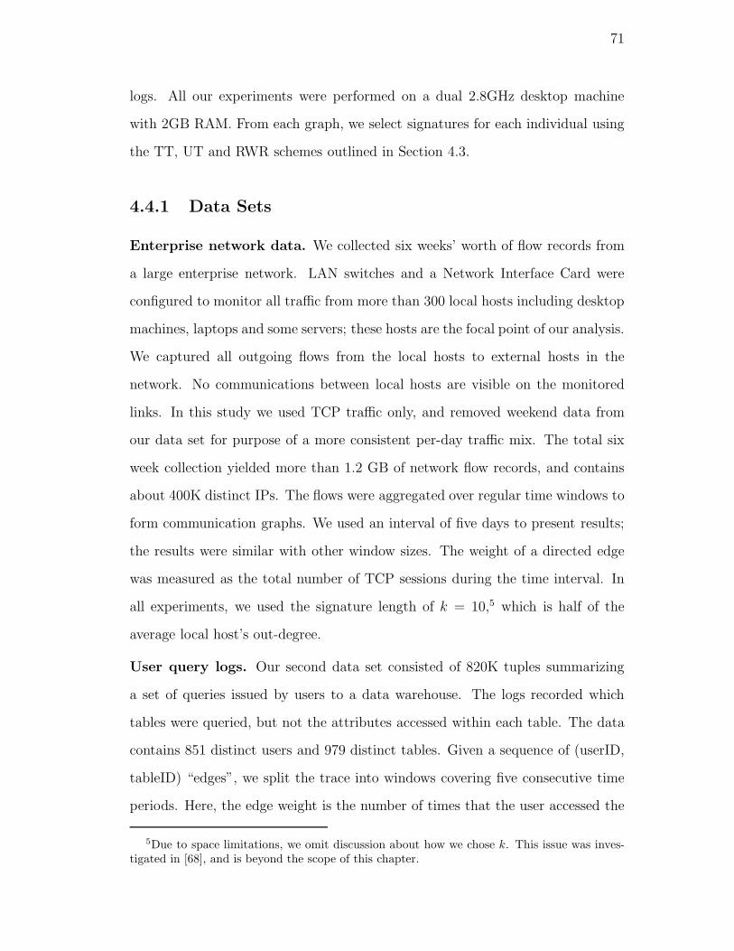
71
logs. All our experiments were performed on a dual 2.8GHz desktop machine
with 2GB RAM. From each graph, we select signatures for each individual using
the TT, UT and RWR schemes outlined in Section 4.3.
4.4.1 Data Sets
Enterprise network data. We collected six weeks’ worth of flow records from
a large enterprise network. LAN switches and a Network Interface Card were
configured to monitor all traffic from more than 300 local hosts including desktop
machines, laptops and some servers; these hosts are the focal point of our analysis.
We captured all outgoing flows from the local hosts to external hosts in the
network. No communications between local hosts are visible on the monitored
links. In this study we used TCP traffic only, and removed weekend data from
our data set for purpose of a more consistent per-day traffic mix. The total six
week collection yielded more than 1.2 GB of network flow records, and contains
about 400K distinct IPs. The flows were aggregated over regular time windows to
form communication graphs. We used an interval of five days to present results;
the results were similar with other window sizes. The weight of a directed edge
was measured as the total number of TCP sessions during the time interval. In
all experiments, we used the signature length of k = 10,5 which is half of the
average local host’s out-degree.
User query logs. Our second data set consisted of 820K tuples summarizing
a set of queries issued by users to a data warehouse. The logs recorded which
tables were queried, but not the attributes accessed within each table. The data
contains 851 distinct users and 979 distinct tables. Given a sequence of (userID,
tableID) “edges”, we split the trace into windows covering five consecutive time
periods. Here, the edge weight is the number of times that the user accessed the
5Due to space limitations, we omit discussion about how we chose k. This issue was inves-tigated in [68], and is beyond the scope of this chapter.
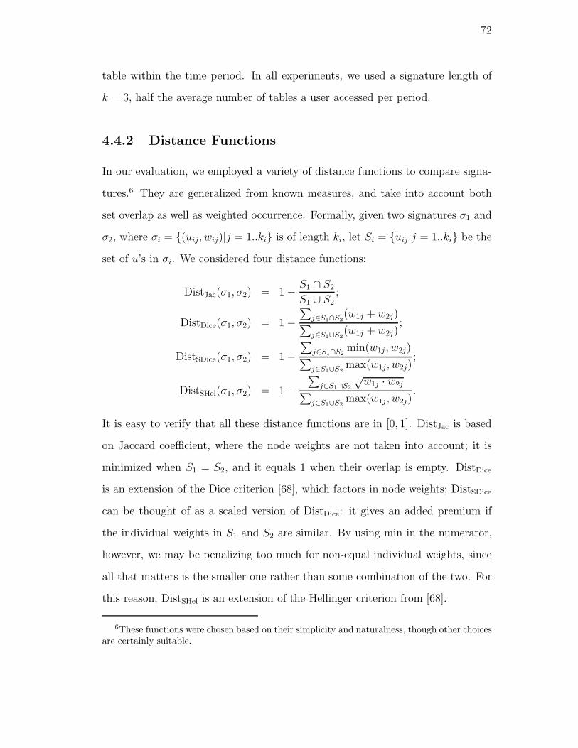
72
table within the time period. In all experiments, we used a signature length of
k = 3, half the average number of tables a user accessed per period.
4.4.2 Distance Functions
In our evaluation, we employed a variety of distance functions to compare signa-
tures.6 They are generalized from known measures, and take into account both
set overlap as well as weighted occurrence. Formally, given two signatures σ1 and
σ2, where σi = {(uij, wij)|j = 1..ki} is of length ki, let Si = {uij|j = 1..ki} be the
set of u’s in σi. We considered four distance functions:
DistJac(σ1, σ2) = 1− S1 ∩ S2
S1 ∪ S2;
DistDice(σ1, σ2) = 1−∑
j∈S1∩S2(w1j + w2j)
∑
j∈S1∪S2(w1j + w2j)
;
DistSDice(σ1, σ2) = 1−∑
j∈S1∩S2min(w1j , w2j)
∑
j∈S1∪S2max(w1j, w2j)
;
DistSHel(σ1, σ2) = 1−∑
j∈S1∩S2
√w1j · w2j
∑
j∈S1∪S2max(w1j, w2j)
.
It is easy to verify that all these distance functions are in [0, 1]. DistJac is based
on Jaccard coefficient, where the node weights are not taken into account; it is
minimized when S1 = S2, and it equals 1 when their overlap is empty. DistDice
is an extension of the Dice criterion [68], which factors in node weights; DistSDice
can be thought of as a scaled version of DistDice: it gives an added premium if
the individual weights in S1 and S2 are similar. By using min in the numerator,
however, we may be penalizing too much for non-equal individual weights, since
all that matters is the smaller one rather than some combination of the two. For
this reason, DistSHel is an extension of the Hellinger criterion from [68].
6These functions were chosen based on their simplicity and naturalness, though other choicesare certainly suitable.
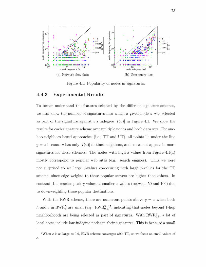
73
100
101
102
100
101
102
node indegrees in G
node
freq
uenc
y in
sig
natu
res
TTUTRWR3
0.1
RWR30.9
y=x
(a) Network flow data
100
101
102
100
101
102
node indegrees in G
node
freq
uenc
y in
sig
natu
res
TTUTRWR3
0.1
RWR30.9
y=x
(b) User query logs
Figure 4.1: Popularity of nodes in signatures.
4.4.3 Experimental Results
To better understand the features selected by the different signature schemes,
we first show the number of signatures into which a given node u was selected
as part of the signature against u’s indegree |I(u)| in Figure 4.1. We show the
results for each signature scheme over multiple nodes and both data sets. For one-
hop neighbors based approaches (i.e., TT and UT), all points lie under the line
y = x because u has only |I(u)| distinct neighbors, and so cannot appear in more
signatures for these schemes. The nodes with high x-values from Figure 4.1(a)
mostly correspond to popular web sites (e.g. search engines). Thus we were
not surprised to see large y-values co-occuring with large x-values for the TT
scheme, since edge weights to these popular servers are higher than others. In
contrast, UT reaches peak y-values at smaller x-values (between 50 and 100) due
to downweighting these popular destinations.
With the RWR scheme, there are numerous points above y = x when both
h and c in RWRhc are small (e.g., RWR3
0.1)7, indicating that nodes beyond 1-hop
neighborhoods are being selected as part of signatures. With RWR30.1, a lot of
local hosts include low-indegree nodes in their signatures. This is because a small
7When c is as large as 0.9, RWR scheme converges with TT, so we focus on small values ofc.
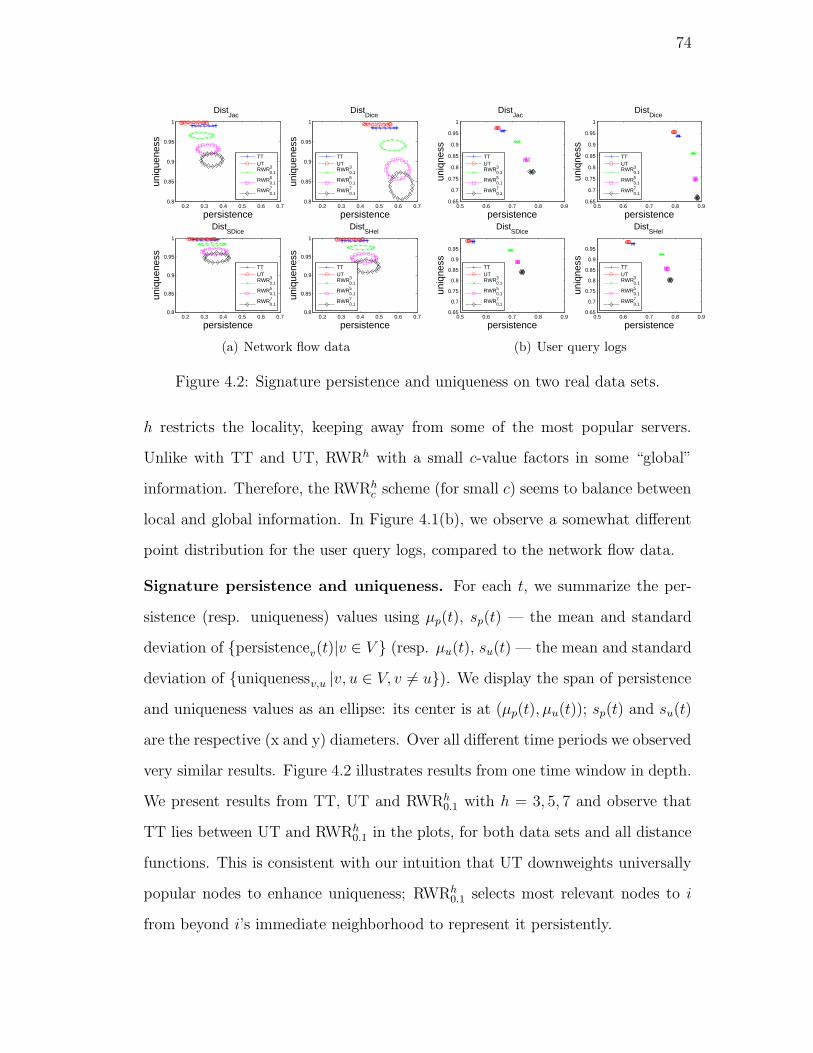
74
0.2 0.3 0.4 0.5 0.6 0.70.8
0.85
0.9
0.95
1
persistence
uniq
uene
ss
DistJac
TTUTRWR3
0.1
RWR50.1
RWR70.1
0.2 0.3 0.4 0.5 0.6 0.70.8
0.85
0.9
0.95
1
persistence
uniq
uene
ss
DistDice
TTUTRWR3
0.1
RWR50.1
RWR70.1
0.2 0.3 0.4 0.5 0.6 0.70.8
0.85
0.9
0.95
1
persistence
uniq
uene
ss
DistSDice
TTUTRWR3
0.1
RWR50.1
RWR70.1
0.2 0.3 0.4 0.5 0.6 0.70.8
0.85
0.9
0.95
1
persistence
uniq
uene
ss
DistSHel
TTUTRWR3
0.1
RWR50.1
RWR70.1
(a) Network flow data
0.5 0.6 0.7 0.8 0.90.65
0.7
0.75
0.8
0.85
0.9
0.95
1
persistence
uniq
ness
DistJac
TTUTRWR3
0.1
RWR50.1
RWR70.1
0.5 0.6 0.7 0.8 0.90.65
0.7
0.75
0.8
0.85
0.9
0.95
1
persistence
uniq
ness
DistDice
TTUTRWR3
0.1
RWR50.1
RWR70.1
0.5 0.6 0.7 0.8 0.90.65
0.7
0.75
0.8
0.85
0.9
0.95
persistence
uniq
ness
DistSDice
TTUTRWR3
0.1
RWR50.1
RWR70.1
0.5 0.6 0.7 0.8 0.90.65
0.7
0.75
0.8
0.85
0.9
0.95
persistence
uniq
ness
DistSHel
TTUTRWR3
0.1
RWR50.1
RWR70.1
(b) User query logs
Figure 4.2: Signature persistence and uniqueness on two real data sets.
h restricts the locality, keeping away from some of the most popular servers.
Unlike with TT and UT, RWRh with a small c-value factors in some “global”
information. Therefore, the RWRhc scheme (for small c) seems to balance between
local and global information. In Figure 4.1(b), we observe a somewhat different
point distribution for the user query logs, compared to the network flow data.
Signature persistence and uniqueness. For each t, we summarize the per-
sistence (resp. uniqueness) values using µp(t), sp(t) — the mean and standard
deviation of {persistencev(t)|v ∈ V } (resp. µu(t), su(t) — the mean and standard
deviation of {uniquenessv,u |v, u ∈ V, v 6= u}). We display the span of persistence
and uniqueness values as an ellipse: its center is at (µp(t), µu(t)); sp(t) and su(t)
are the respective (x and y) diameters. Over all different time periods we observed
very similar results. Figure 4.2 illustrates results from one time window in depth.
We present results from TT, UT and RWRh0.1 with h = 3, 5, 7 and observe that
TT lies between UT and RWRh0.1 in the plots, for both data sets and all distance
functions. This is consistent with our intuition that UT downweights universally
popular nodes to enhance uniqueness; RWRh0.1 selects most relevant nodes to i
from beyond i’s immediate neighborhood to represent it persistently.
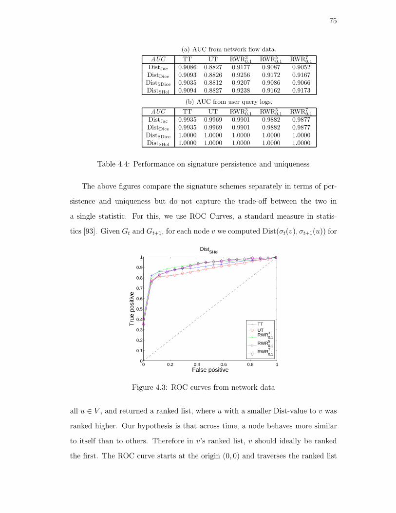
75
(a) AUC from network flow data.
AUC TT UT RWR30.1 RWR5
0.1 RWR70.1
DistJac 0.9086 0.8827 0.9177 0.9087 0.9052DistDice 0.9093 0.8826 0.9256 0.9172 0.9167DistSDice 0.9035 0.8812 0.9207 0.9086 0.9066DistSHel 0.9094 0.8827 0.9238 0.9162 0.9173
(b) AUC from user query logs.
AUC TT UT RWR30.1 RWR5
0.1 RWR70.1
DistJac 0.9935 0.9969 0.9901 0.9882 0.9877DistDice 0.9935 0.9969 0.9901 0.9882 0.9877DistSDice 1.0000 1.0000 1.0000 1.0000 1.0000DistSHel 1.0000 1.0000 1.0000 1.0000 1.0000
Table 4.4: Performance on signature persistence and uniqueness
The above figures compare the signature schemes separately in terms of per-
sistence and uniqueness but do not capture the trade-off between the two in
a single statistic. For this, we use ROC Curves, a standard measure in statis-
tics [93]. Given Gt and Gt+1, for each node v we computed Dist(σt(v), σt+1(u)) for
0 0.2 0.4 0.6 0.8 10
0.1
0.2
0.3
0.4
0.5
0.6
0.7
0.8
0.9
1
False positive
Tru
e po
sitiv
e
DistSHel
TTUTRWR3
0.1
RWR50.1
RWR70.1
Figure 4.3: ROC curves from network data
all u ∈ V , and returned a ranked list, where u with a smaller Dist-value to v was
ranked higher. Our hypothesis is that across time, a node behaves more similar
to itself than to others. Therefore in v’s ranked list, v should ideally be ranked
the first. The ROC curve starts at the origin (0, 0) and traverses the ranked list

76
of nodes from the top. If the element is v, the ROC curve goes up by a step of
1; otherwise, the ROC curve goes to the right by a step of 1/(|V | − 1). That is,
the x-axis is false positives and y-axis is true positives. We can then compute
the Area Under the ROC Curve (AUC). If the AUC is 0.5, the signature scheme
is no better than random selection; higher AUC values indicate better accuracy,
up to 1 (perfect). We report the average AUC over all v’s. Figure 4.3 shows the
results on the flow data using DistSHel; ROC curves from other distance measures
look very similar.
Table 4.3(a) summarizes AUC across different signature schemes per distance
measure for the flow data. The multi-hop neighbors based schemes achieved bet-
ter AUCs than their one-hop counterparts. Among RWRh0.1 schemes, RWR3
0.1
outperformed the other two. A further observation is that the difference between
the AUC from RWR50.1 and RWR7
0.1 is small enough to be ignored. Other exper-
iments (not shown) with RWRh0.1 for h > 7 all converged to RWR7
0.1, suggesting
that having more than 5 hops does not bring in drastically “new information”.
This is due in part to the graph having a small diameter: for all h larger than
the diameter of the graph, RWRh coincides with RWR∞, the unbounded random
walk. We repeated the same experiments on user query logs, and summarize AUC
values in Table 4.3(b). All signature schemes behave almost equally well on this
data set (almost perfectly), with UT being slightly better than the others. In
what follows we use RWR30.1 as the best representative of the RWR schemes, and
do not show results for other parameter settings.
Signature robustness. To evaluate the robustness of the signature schemes, we
randomly inserted and deleted edges to obtain a perturbed graph G′t. Let σ(v)
and σ(v) denote v’s signatures constructed from Gt and G′t, respectively. Given
a bipartite graph Gt and parameter α, we inserted α|Et| new edges. First, a
node v′ ∈ V1 was sampled proportional to its outdegree, that is, with probability
|O(v′)|/∑v |O(v)|. Then a node u′ ∈ V2 was sampled proportional to its indegree,
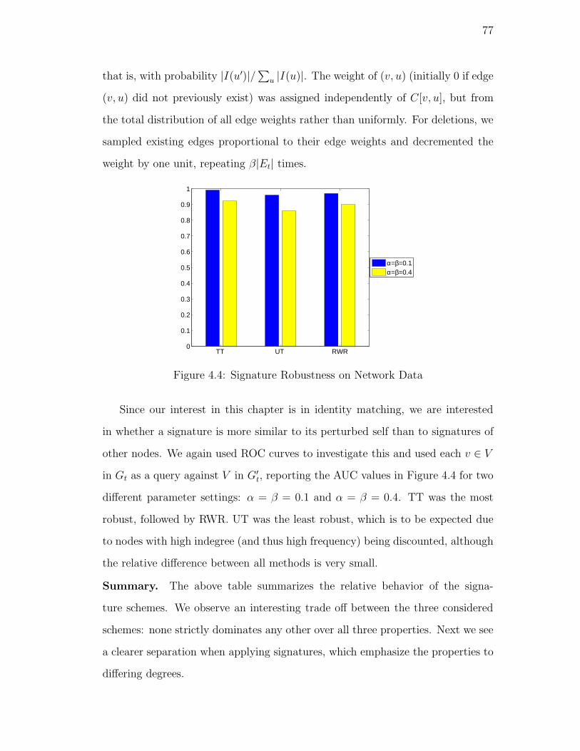
77
that is, with probability |I(u′)|/∑u |I(u)|. The weight of (v, u) (initially 0 if edge
(v, u) did not previously exist) was assigned independently of C[v, u], but from
the total distribution of all edge weights rather than uniformly. For deletions, we
sampled existing edges proportional to their edge weights and decremented the
weight by one unit, repeating β|Et| times.
TT UT RWR0
0.1
0.2
0.3
0.4
0.5
0.6
0.7
0.8
0.9
1
α=β=0.1α=β=0.4
Figure 4.4: Signature Robustness on Network Data
Since our interest in this chapter is in identity matching, we are interested
in whether a signature is more similar to its perturbed self than to signatures of
other nodes. We again used ROC curves to investigate this and used each v ∈ V
in Gt as a query against V in G′t, reporting the AUC values in Figure 4.4 for two
different parameter settings: α = β = 0.1 and α = β = 0.4. TT was the most
robust, followed by RWR. UT was the least robust, which is to be expected due
to nodes with high indegree (and thus high frequency) being discounted, although
the relative difference between all methods is very small.
Summary. The above table summarizes the relative behavior of the signa-
ture schemes. We observe an interesting trade off between the three considered
schemes: none strictly dominates any other over all three properties. Next we see
a clearer separation when applying signatures, which emphasize the properties to
differing degrees.
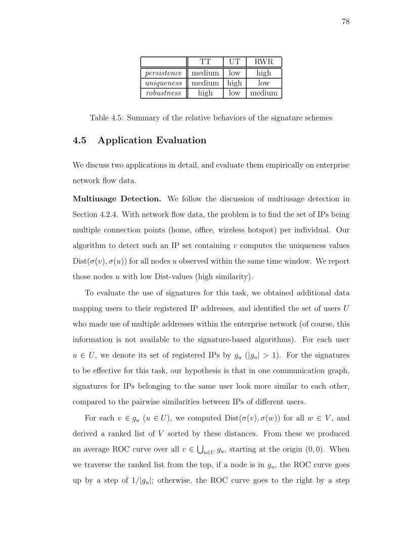
78
TT UT RWR
persistence medium low highuniqueness medium high lowrobustness high low medium
Table 4.5: Summary of the relative behaviors of the signature schemes
4.5 Application Evaluation
We discuss two applications in detail, and evaluate them empirically on enterprise
network flow data.
Multiusage Detection. We follow the discussion of multiusage detection in
Section 4.2.4. With network flow data, the problem is to find the set of IPs being
multiple connection points (home, office, wireless hotspot) per individual. Our
algorithm to detect such an IP set containing v computes the uniqueness values
Dist(σ(v), σ(u)) for all nodes u observed within the same time window. We report
those nodes u with low Dist-values (high similarity).
To evaluate the use of signatures for this task, we obtained additional data
mapping users to their registered IP addresses, and identified the set of users U
who made use of multiple addresses within the enterprise network (of course, this
information is not available to the signature-based algorithms). For each user
u ∈ U , we denote its set of registered IPs by gu (|gu| > 1). For the signatures
to be effective for this task, our hypothesis is that in one communication graph,
signatures for IPs belonging to the same user look more similar to each other,
compared to the pairwise similarities between IPs of different users.
For each v ∈ gu (u ∈ U), we computed Dist(σ(v), σ(w)) for all w ∈ V , and
derived a ranked list of V sorted by these distances. From these we produced
an average ROC curve over all v ∈ ⋃u∈U gu, starting at the origin (0, 0). When
we traverse the ranked list from the top, if a node is in gu, the ROC curve goes
up by a step of 1/|gu|; otherwise, the ROC curve goes to the right by a step
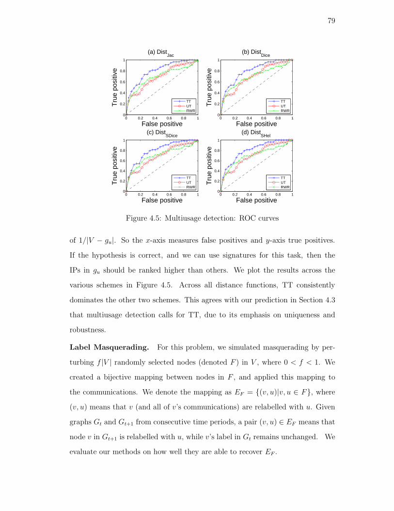
79
0 0.2 0.4 0.6 0.8 10
0.2
0.4
0.6
0.8
1
False positiveT
rue
posi
tive
(a) DistJac
TTUTRWR
0 0.2 0.4 0.6 0.8 10
0.2
0.4
0.6
0.8
1
False positive
Tru
e po
sitiv
e
(b) DistDice
TTUTRWR
0 0.2 0.4 0.6 0.8 10
0.2
0.4
0.6
0.8
1
False positive
Tru
e po
sitiv
e
(c) DistSDice
TTUTRWR
0 0.2 0.4 0.6 0.8 10
0.2
0.4
0.6
0.8
1
False positiveT
rue
posi
tive
(d) DistSHel
TTUTRWR
Figure 4.5: Multiusage detection: ROC curves
of 1/|V − gu|. So the x-axis measures false positives and y-axis true positives.
If the hypothesis is correct, and we can use signatures for this task, then the
IPs in gu should be ranked higher than others. We plot the results across the
various schemes in Figure 4.5. Across all distance functions, TT consistently
dominates the other two schemes. This agrees with our prediction in Section 4.3
that multiusage detection calls for TT, due to its emphasis on uniqueness and
robustness.
Label Masquerading. For this problem, we simulated masquerading by per-
turbing f |V | randomly selected nodes (denoted F ) in V , where 0 < f < 1. We
created a bijective mapping between nodes in F , and applied this mapping to
the communications. We denote the mapping as EF = {(v, u)|v, u ∈ F}, where
(v, u) means that v (and all of v’s communications) are relabelled with u. Given
graphs Gt and Gt+1 from consecutive time periods, a pair (v, u) ∈ EF means that
node v in Gt+1 is relabelled with u, while v’s label in Gt remains unchanged. We
evaluate our methods on how well they are able to recover EF .

80
Algorithm 2 DetectLabelMasquerading(Gt, Gt+1)
1: Init V1 = ∅, OF = ∅.2: for each v ∈ V do
3: if 1−Dist(σt(v), σt+1(v)) > δ then
4: V1 = V1 ∪ {v}5: else
6: ∀u ∈ V , M [u, v] = 1−Dist(σt(v), σt+1(u))7: if ∃u 6= v, M [v, u] is among v’s top-ℓ largest and M [u, u] ≤ δ then
8: OF = OF ∪ {(v, u)}9: else
10: V1 = V1 ∪ {v}11: end if
12: end if
13: end for
Based on the discussion in Section 4.2.4, the detection algorithm is given in
pseudo-code in Algorithm 2. Here V1 returns the set of local hosts not identified
as masqueraders; OF is the estimate for EF . We see that an output (v, u) satisfies
two conditions: (1) both v and u look different from themselves across time (i.e.,
low persistence values, from Step 3 and 7 in Algorithm 2); but (2) they look more
similar to each other than to others (i.e., high persistence between themselves,
from Step 7). We evaluate the various signature schemes for this problem based on
the standard information retrieval criteria of precision, recall and accuracy. Here,
accuracy measures the percentage of correctly classified hosts, labeled either as
“non-suspect” (i.e., v /∈ F ) or with the new label of the node. This combines
notions of false positives and false negatives, so we use it as our main evaluation
criterion.
In our algorithm, the persistency threshold δ should be a good cutoff between
local hosts whose signatures look persistent and those who are not. Therefore,
we set δ experimentally as δ =P
v∈V (1−Dist(σt(v),σt+1(v)))
p|V |, p ∈ N. That is, we chose
δ as a fraction of the average self-similarity across time (scaled down by p). In
particular, we considered p = 3, 5, 7 in our experiments, and observed very similar
results. Figure 4.6 compares the performance of various schemes with p = 5, for
various ℓ-values, as a function of fraction of the nodes perturbed.
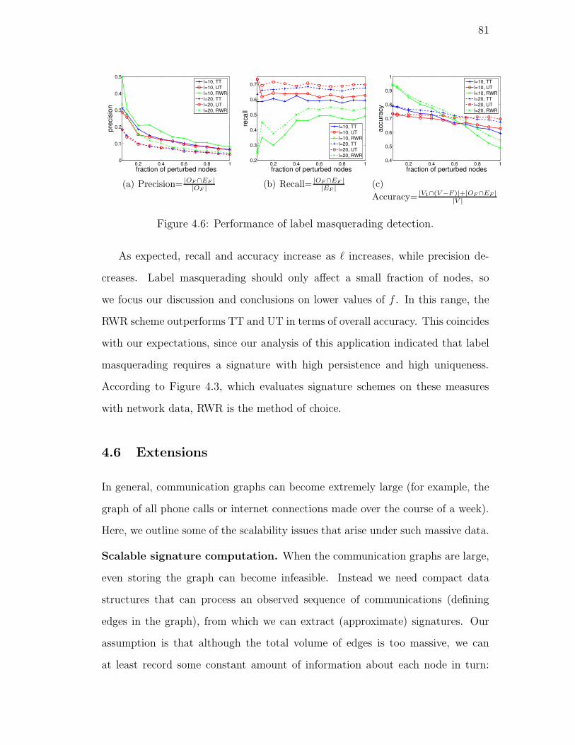
81
0.2 0.4 0.6 0.8 10
0.1
0.2
0.3
0.4
0.5
fraction of perturbed nodes
pre
cis
ion
l=10, TT
l=10, UT
l=10, RWR
l=20, TT
l=20, UT
l=20, RWR
(a) Precision= |OF∩EF ||OF |
0.2 0.4 0.6 0.8 10.2
0.3
0.4
0.5
0.6
0.7
fraction of perturbed nodes
reca
ll
l=10, TT
l=10, UT
l=10, RWR
l=20, TT
l=20, UT
l=20, RWR
(b) Recall= |OF ∩EF ||EF |
0.2 0.4 0.6 0.8 10.4
0.5
0.6
0.7
0.8
0.9
1
fraction of perturbed nodes
accu
racy
l=10, TT
l=10, UT
l=10, RWR
l=20, TT
l=20, UT
l=20, RWR
(c)
Accuracy= |V1∩(V −F )|+|OF ∩EF ||V |
Figure 4.6: Performance of label masquerading detection.
As expected, recall and accuracy increase as ℓ increases, while precision de-
creases. Label masquerading should only affect a small fraction of nodes, so
we focus our discussion and conclusions on lower values of f . In this range, the
RWR scheme outperforms TT and UT in terms of overall accuracy. This coincides
with our expectations, since our analysis of this application indicated that label
masquerading requires a signature with high persistence and high uniqueness.
According to Figure 4.3, which evaluates signature schemes on these measures
with network data, RWR is the method of choice.
4.6 Extensions
In general, communication graphs can become extremely large (for example, the
graph of all phone calls or internet connections made over the course of a week).
Here, we outline some of the scalability issues that arise under such massive data.
Scalable signature computation. When the communication graphs are large,
even storing the graph can become infeasible. Instead we need compact data
structures that can process an observed sequence of communications (defining
edges in the graph), from which we can extract (approximate) signatures. Our
assumption is that although the total volume of edges is too massive, we can
at least record some constant amount of information about each node in turn:

82
this is the “semi-streaming” model of graph stream processing [96]. Any given
signature scheme will need a different approach in this restricted model, here
we outline methods for the signature schemes used here for illustration. For the
Top Talkers, we need to find the approximate heaviest-weight neighbors of node
i. If the communication is pre-aggregated, we can just keep a heap of heavy
edges; but more realistically, we see each individual communication, and want to
recover the most frequent. We can use summary structures such as a CM sketch
for each node to find its heaviest outgoing edges, and hence its signature [30]. For
Unexpected Talkers, the situation is more complex. Here, we can additionally
keep an FM sketch for each node, to find its incoming degree [51]. To find the
signature for a node i, we can use the CM sketch to estimate C[i, j], and the FM
sketch to estimate |I(j)| for each node j; combining these gives an approximation
of C[i, j]/|I(j)| as required. For schemes based on Random Walk with Reset,
there is less prior work to draw on. Techniques in [107] give approaches to make
the comptuations more scalable, based on appropriate block-wise decompositions
of the graph; extending these to the full semi-streaming model remains an open
problem.
Scalable signature comparison. When there are large number of nodes with
signatures, applications based on comparing many signatures together become
expensive (potentially quadratic in the number of nodes). At the heart of many
applications discussed above is the problem of, given a signature, finding the most
similar signature(s) from a particular (sub)set. This fits the set up of the nearest
neighbor problem. Even for moderately small signature sizes, this can become
expensive, and so we can turn to approximate nearest neighbor algorithms. Here,
different approaches are needed for each different distance function, rather than
signature scheme. For example, efficient solutions exist where the distance func-
tion is the Jacard distance, by using an approach based on Locality Sensitive
Hashing [75].

83
4.7 Related Work
Signatures (and fingerprints) were classically studied as an application of statis-
tical pattern recognition, an area of study with a long history of techniques for
feature selection and classification [77]. However, these generic techniques are less
appropriate given contextual information as in the case of communication graphs.
Usage profiling in graphs (and networks) has been studied in multiple set-
tings [99, 117, 85, 107, 73, 98]. However, the goal of these works is to model behav-
ior aggregated at the level of the entire graph to detect network-wide anomalies.
Usage profiling at the granularity of the individual has been studied for activity
monitoring [48], for user recognition [106], and for enterprise security [83]. The
approach uses complex rules on records of individual activity requiring detailed
data storage.
Cortes et al. initiated the study of “COI-based” signatures, which makes use
of communication graph topology to design individual’s signatures in a concise
way for detecting fraudulent users [35, 36], identifying repetitive debtors [68] and
predicting links for viral marketing [70]; similar techniques were also applied to
identify authors from bibliographical citations in [69]. However, they only focused
on particular signatures and their applicability to the motivating tasks. We do
not know of any prior work that proposed a principled approach such as ours
for a detailed classification of properties of signatures and studying applications
based on what properties they need for signatures to be useful.
4.8 Chapter Summary
Nowadays interaction or communication between individuals is ubiquitous. Given
this abundance of communication, many applications emerge which rely on ana-
lyzing the patterns behind the communications. The idea of using signatures to
capture behavior is an attractive one. Here, we have attempted to take a very

84
general approach to problems of defining and analyzing signatures in communica-
tion graphs. We proposed a general framework for understanding and analyzing
these signatures, based on the three fundamental and natural properties of persis-
tence, uniqueness and robustness. We justified these properties by showing how
they impact a broad set of applications. We explored several signature schemes in
our framework and evaluated them on real data in terms of these properties. In
particular, our study on two concrete applications using signatures demonstrates
their effectiveness on real data experimentally. This study underlined the fact
that there is not one single signature scheme which is good for all applications,
but rather that different signatures are needed, depending on what balance of
the three properties they provide. We believe that a larger suite of properties
of signatures are needed for the space of all applications that signatures will be
useful for.

85
Chapter 5
Modeling Distributional Changes via Sequential
Probability Ratio Test
5.1 Introduction
Model-based declarative queries are becoming an attractive paradigm for inter-
acting with many data stream applications. This has led to the development of
techniques to accurately answer the queries using distributional models rather
than raw values. The quintessential problem with this is that of detecting when
there is a change in the input stream [53, 72, 111], which makes models stale and
inaccurate. In IP network management, changes in the traffic patterns might
indicate an intrusion, attack or an anomaly that needs attention of the network
managers [79, 84, 31]. Likewise in financial streams, a change in the pattern of
trades might represent an opportunity or a warning for the analyst.
In particular, changes may be global, involving the entire distribution of items
(such as determining if the distributions are far apart in some measure), or local,
involving the distribution of singleton items (such as, if individual probability
differs significantly in one distribution to another).
Change detection between two stored data sets in general brings up fundamen-
tal questions such as how to measure change and what is a threshold for change.
In the context of data streams, additional questions arise. In particular, what
are the “two” data sets that would be basis for detecting a change? Typically,
data stream queries specify some window W on which the query is executed. For
example, there are tumbling window queries or sliding window queries [96, 9]. An

86
issue is how to determine the W . Although the need of continuous detection
for changes gives rise to the sliding window model [80, 39], in change detection
problems, fixing a window size can only work well if information on the time-scale
of change is available, but this is rarely the case. Indeed, we need scale-free de-
tection algorithm to find changes as quickly as possible. However, this goal may
be delayed by the size of the window, since a window smaller than the changing
rate may miss the detection or capture the change at a later time when gradual
changes cumulate over time, and a window larger than the changing rate delays
the detection until the end of the window. One can tradeoff some performance by
searching over multiple sliding windows (of different sizes) in parallel by spending
some analysis time and space [80, 39]. But it is infeasible to exhaustively search
over all possible window sizes. A different strategy uses a decaying-weighted win-
dow [84, 40] to weight the importance of examples according to their age. In this
case, the choice of a decay constant should match the unknown rate of change.
Still, what is needed is a seamless change detection method, such that whenever
a change occurs, it accurately estimates when it happens with short detection
delay.
In this chapter, we present such change detection algorithms that are inspired
by the well-known sequential probability ratio test [109, 14] in Statistics. It comes
with sound basis for setting the threshold for change, for providing guarantees
on keeping track of the change point incrementally and for the minimum delay in
detecting a change, under the assumptions that (1) distributions before and after
a change are both known as a priori; (2) observations are generated independently.
Our algorithmic contribution is to design a very space-efficient, yet fast method
for change detection in one pass over the data streams, where we have to relax the
above two assumptions. Furthermore, we show that it not only holds for global
changes in the distributions as is studied in Statistics, but also holds for local
changes that have not been addressed earlier. We perform a thorough study of

87
our algorithms in practice with synthetic and real data sets. We not only show the
accuracy and robustness of our algorithms to detect changes in one pass, but also
demonstrate the accurate change-point estimate, relative to those obtained offline.
Our approaches have short detection delay, compared to alternative window-based
solutions. Finally, we study real traces with web logs to demonstrate how an
accurate change-point estimate can help improve model-based query qualities.
Another case study with labelled attacks shows experimental evidence that our
methods have the potential power for intrusion detection monitoring. Still, better
understanding of how attacks incur changes is needed to infer critical things.
The chapter is organized as follows. We define both global and local change
detection problems in Section 5.2. We present our global change detection algo-
rithms in Section 5.3 and present experimental studies in Section 5.5. Likewise,
we present algorithmic methods and experimental studies in Section 5.4 and 5.6
respectively for local change detection. Related work is in Section 5.7, with con-
clusions in Section 5.8.
5.2 Change Detection Problems
An1 = (x1 . . . xn) is a sequence of input items, with xi ∈ U = {0..u−1}, generated
from some underlying distribution at time i. Its sub-sequence Aw1 = (x1 . . . xw),
w < n, is a baseline data set generated from an original distribution P0. With P0
known as a priori, two situations are possible: either every xi ∈ An1 is generated
from P0, or there exists an unknown change point w < λ ≤ n such that, xi ∼ P0
for i < λ and xi ∼ P1 for w < λ ≤ i ≤ n, where P0 and P1 are called pre- and
post-change distributions. We say that a change in P0 has occurred if P1 differs
significantly from P0. By significance we mean the amount of change, measured by
a distance function Dλ(P1||P0), is greater than some threshold. Here Dλ(P1||P0)
depends on the change point λ.

88
A change detection problem is based on hypotheses: H0 — there is no change
in P0; and H1, otherwise. Here H1 is a composite of a set of “parallel” tests
{Hλ|w < λ ≤ n}, where Hλ is the hypothesis that a change occurs at time λ;
that is, H1 =⋃
w<λ≤n Hλ. In one pass over the data streams, data is presented
one point at a time. To quickly detect a change after its occurrence, the best
opportunity is to make a declaration after each observation, in the process of
data acquisition. Therefore at each xn, a desired change detection algorithm
operates in two phases: it first locates an index w < λ ≤ n, which has the highest
probability of being a change point (i.e., the largest Dλ(P1||P0)); in the second
phase, we conduct a hypothesis testing to accept or reject λ as a change point
(i.e. to accept or reject H1). To interpret the change, the hypothesis testing
compares the largest Dλ(P1||P0) against a threshold to tell whether the difference
is significant. Once we accept Hλ at time n, we call λ the change point, and n the
change detection point; otherwise, we continue to make an additional observation.
Formally,
Definition 6 Let (x1, ..., xn) be an input stream, and its sub-stream (x1, ..., xw),
w < n, is generated from a prior distribution P0. A change detection problem is
to decide whether to accept H1 (i.e., reject H0) or not. We accept H1 at time n
when
• A global change in entire distribution is detected when
T n = Dλ∗(P1||P0) = maxw<λ≤n
Dλ(P1||P0) ≥ τg,
• A local change in distribution of a singleton item j ∈ U is detected when
T n = Dλ∗(P1[j]||P0[j]) = maxw<λ≤n
Dλ(P1[j]||P0[j]) ≥ τl,
where τg and τl are global and local change detection threshold to be specified in
Section 5.3.1 and 5.4. A change detection algorithm outputs: λ∗ = arg maxw<λ≤n Dλ(P1||P0)
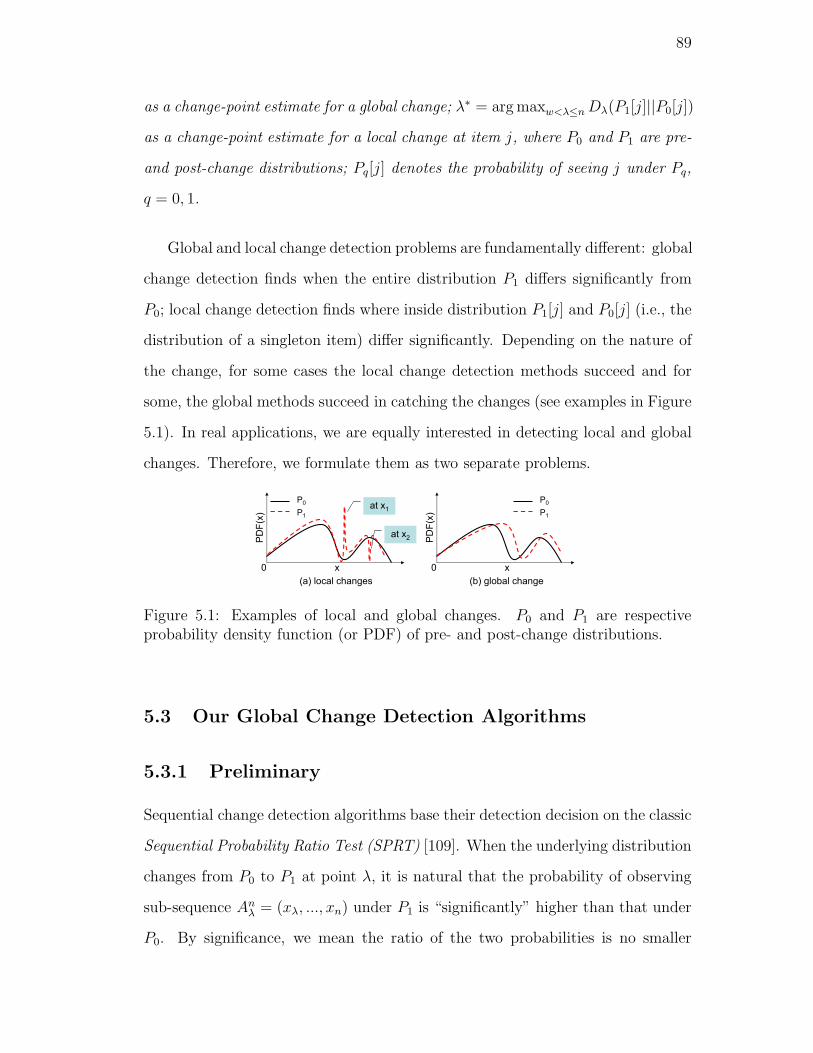
89
as a change-point estimate for a global change; λ∗ = arg maxw<λ≤n Dλ(P1[j]||P0[j])
as a change-point estimate for a local change at item j, where P0 and P1 are pre-
and post-change distributions; Pq[j] denotes the probability of seeing j under Pq,
q = 0, 1.
Global and local change detection problems are fundamentally different: global
change detection finds when the entire distribution P1 differs significantly from
P0; local change detection finds where inside distribution P1[j] and P0[j] (i.e., the
distribution of a singleton item) differ significantly. Depending on the nature of
the change, for some cases the local change detection methods succeed and for
some, the global methods succeed in catching the changes (see examples in Figure
5.1). In real applications, we are equally interested in detecting local and global
changes. Therefore, we formulate them as two separate problems.
PD
F(x
)
x0
P0
P1
(b) global change
PD
F(x
)
x0
P0
P1
(a) local changes
at x1
at x2
Figure 5.1: Examples of local and global changes. P0 and P1 are respectiveprobability density function (or PDF) of pre- and post-change distributions.
5.3 Our Global Change Detection Algorithms
5.3.1 Preliminary
Sequential change detection algorithms base their detection decision on the classic
Sequential Probability Ratio Test (SPRT) [109]. When the underlying distribution
changes from P0 to P1 at point λ, it is natural that the probability of observing
sub-sequence Anλ = (xλ, ..., xn) under P1 is “significantly” higher than that under
P0. By significance, we mean the ratio of the two probabilities is no smaller

90
than a threshold. Given that both P0 and P1 are known as a priori, and that
points in the stream are independently generated, the test statistic for testing the
hypothesis Hλ that a change occurrs at time λ against H0 that there is no change
is equal to
T nλ = Dλ(P1||P0) = log
Pr(xλ...xn|P1)
Pr(xλ...xn|P0)
=n∑
i=λ
logP1[xi]
P0[xi]= T n−1
λ + logP1[xn]
P0[xn].
Page’s (CUSUM) procedure [14] identifies that the statistic T n = maxw<λ≤n T nλ
obeys the recursion (T 0 = 0):
T n = max
(
0, T n−1 + logP1[xn]
P0[xn]
)
.
Therefore, it takes each new item O(1) time to update T n and to detect a global
change by testing T n ≥ τg. Accordingly, we update the most likely change point
to n in O(1) time when T n = 0, without extra overhead. When a change is
detected at time n, the change-point estimate is λ∗ = max{λ|T λ = 0, w < λ ≤n}. Therefore, the adaptive window size at time n is w(n) = w(n−1) · 1{T n>0} +
1, where 1{x} is the indicator of event x, w(n) is the number of observations
after the last time the test statistic T n is reset to zero, and the start point of
the so-called adaptive window estimates the change point. In addition, Wald’s
approximation [109] says that global threshold τg = log((1 − β)/α), given user-
specified false alarm rate α = Pr(H1|H0) = Pr(T n ≥ τg|H0) and miss detection
rate β = Pr(H0|H1) = Pr(T n < τg|H1).
Here T n is an integration of the log likelihood ratios of the most recent (n−λ + 1) observations, such that T n
λ is maximized. Thus, it is inherent that only
items after the change point contribute to T n. And the natural advantage of this
statistic is to detect changes at different scales without instantiating windows of
different sizes in parallel.
91
5.3.2 Our Offline Algorithm
All discussions in Section 5.3.1 assume that both P0 and P1 are known as a priori.
In practice, it is fair to assume the availability of a “base” distribution P0, but not
the prior knowledge of P1. So (1) how to derive the post-change distribution P1
from the stream? How to incrementally maintain it? (2) What if observations in
stream are not independent, just as with streaming data? We shall address these
issues in this Section. For streaming concerns, we design a fast and small-space
algorithm in Section 5.3.3.
In the context of our problem, the input is a sequence of points An1 = (x1 . . . xw . . . xn);
each xi ∈ U . The original distribution P0 is known as a priori, and is constructed
from the first w observations Aw1 = (x1 . . . xw). It is defined as a vector represent-
ing the relative frequency of each distinct element j ∈ U , with smoothing:
P0[j] =|{i|xi = j, 1 ≤ i ≤ w}|+ γ
w + γ · u =Sw
1 [j] + γ
w + γ · u .
Here Sw1 [j] denotes the frequency for item j in Aw
1 . γ is usually set to 0.5
for smoothing, which controls the sensitivity to previously unseen items (i.e.,
∀j ∈ U, P0[j] > 0); u = |U | is the domain size. We assume that the size w of
the baseline data set is large enough to guarantee the goodness of P0, compared
to its true counterpart. There are a variety of methods to capture the under-
lying distribution of a sequence. For simplicity and popularity reasons, we use
empirical distributions after smoothing throughout the chapter. However, our
change detection methodology, as a whole, fits well with other alternatives. That
is, we can isolate definition of a change and mechanism to detect it from the data
representation itself.
Our P1 is incrementally updated based on P0 with new arrivals; that is at
any time n, P n1 is derived from An
1 : ∀j ∈ U , P n1 [j] =
Sn1 [j]+γ
n+γ·u. An inherent
problem with this setup is that when a change occurs, P1 constructed based on
all observations An1 makes use of stale data, thus is reluctant to reflect the change

92
promptly. Our argument is that having a change-point-dependent test statistic
greatly alleviates such detection delays. We will study the effectiveness of this
setup against alternative solutions in experiments. In practice, we can improve
our algorithm by adopting, for example sliding window [40] or decaying window
[27] models, to build more up-to-date P1. We consider such variants orthogonal
to our main line of inquiry, and do not consider it explicitly any further.
Theorem 7 With dependent observations, T nλ ≃ Zn
λ =∑n
i=λ logP i
1[xi]
P0[xi], where
P i1[xi] =
Si1[xi]+γ
i+γ·u; Si
1[xi] = |{j|xj = xi, 1 ≤ j ≤ i}|; the smoothing factor γ = 0.5;
u = |U |.
Proof. According to the definition for T nλ ,
T nλ = log
Pr(xλ...xn|P1)
Pr(xλ...xn|P0)
= logPr(xn|xλ...xn−1, P1) · Pr(xλ...xn−1|P1)
Pr(xn|xλ...xn−1, P0) · Pr(xλ...xn−1|P0)
≃ log
∏ni=λ P i
1[xi]∏n
i=λ P0[xi]=
n∑
i=λ
logP i
1[xi]
P0[xi]
≡ Znλ = Zn−1
λ + logP n
1 [xn]
P0[xn].
The second equality holds due to Bayes’s rule; “≃” means asymptotically equal
since i ≥ λ > w ≫ 0, and holds according to the definition for P i1 and the fact
that observations xλ . . . xn are independent under a priori P0.
The proof shows that the incremental maintenance of test statistics is by no
means restricted to the independence assumption. It is generally true even for
dependent observations. Again, test statistic Zn = maxw<λ≤n Znλ for our offline
global change detection algorithm obeys the recursion (Z0 = 0):
Zn = max
(
0, Zn−1 + logP n
1 [xn]
P0[xn]
)
.
Figure 5.2 illustrates the basic structure of the algorithm: “base” distribution
P0 is derived from (x1 . . . xw) as a priori; P n1 is the empirical distribution over

93
- Elements
- Time
x1 x2 xw…xw+1 x…
xn…
P0
P1n
Zn
- Empirical
distributions
- Test statistic
most likely change point
Figure 5.2: An illustration for the sequential change detection algorithm.
(x1 . . . xn); test statistic Zn integrates the change-point estimate and is evaluated
incrementally only according to points after the change. Formally, at any time n:
1. It takes Θ(1) time to update Sn1 [xn]← Sn−1
1 [xn] + 1 and P n1 [xn].
2. It takes Θ(1) time to update test statistic Zn according to the recursion.
If Zn ≥ τg, report a detected global change and the associated most likely
change point λ∗. Otherwise, if Zn = 0, update λ∗ = n.
Theorem 8 Our offline sequential change detection algorithm takes O(u) space
and O(1) per-item processing time to detect a global change, where u = |U |.
Proof. It takes O(u) space to store Sw1 and Sn
1 exactly, plus another two words
of memory for respective Zn and λ∗.
5.3.3 Streaming Algorithm
We will use previously known sketches [96, 9] as basic components to summarize
the input in small space. Then we will estimate test statistic Zn and most likely
change point λ∗ from such small-space structures. One simple attempt is to create
sketches for Sw1 and Sn
1 , hence to derive good estimates for P0 and P n1 , respectively.
For every new item xn, the estimate for test statistic Zn is updated through
Zn = max(
0, Zn−1 + log P1n[xn]
P0[xn]
)
. However, this method is severely flawed in
two ways. First, approximating the ratio of values in small space could perform
poorly, although we have accurate estimates for values. Second, even though
94
we obtain accurate estimate per log-ratio, the additive errors accumulated with
infinite new items might lead to unbounded errors. Therefore, a more careful
design of a streaming algorithm is desired.
High-level ideas. Since the simple combination of incremental updates (via
recursion) and sketches fails to accurately detect changes, we focus on designing
a sketch-based algorithm to estimate test statistic Zn directly in polylogarithmic
time per item. Although this is slightly weaker, compared to the offline algo-
rithm’s O(1) per-item processing time, we have immediate gain in space. Unlike
with the offline solution, we do not incrementally update Zn, neither does λ∗.
Thus, we will derive λ∗ based on multiple Znλ estimates. Instead of exhausting
all w < λ ≤ n (i.e., O(n)) points and taking the max, we probe at values of the
change point λ that form a geometric progression. For example, we may estimate
Znλ only for λ = n, n − 1, n− 2, n− 4, . . . , n − 2i, . . .. The justification is that it
achieves a dramatic reduction in computation time, since we need only O(log n)
estimates to keep track of. Our method will give good accuracy for λ closer to
n, exactly because for such λ’s we have many points to interpolate; it may give a
larger error for λ≪ n, but the relative error will probably be small.
Data structures. In order to obtain a good estimate for test statistics in form
of log likelihood ratios, we need to pre-process Aw1 = (x1 . . . xw) to be aggregated
to Sw1 [i] = |j|xj = i, 1 ≤ j ≤ w|. And this is feasible due to our prior knowledge
on P0. As for streaming algorithm, let S1/P0be the stream whose ith entry is
S1/P0 [i] = 1P0[i]
= w+γ·uSw
1 [i]+γ. We keep a CM sketch (see Section 2.2.1) for this
“inverted” stream, denoted CM1/P0 . It can be shown that ∀i ∈ U , CM1/P0 [i] =
minj count[j, hj(i)] is a good estimate for 1/P0[i].
On the other hand, we will use EH+CM to summarize An1 = (x1 . . . xn),
such that we can use it to answer point queries Snλ [i], for any 1 ≤ λ ≤ n, with
accuracy guarantees. We refer to this structure by EHCMS1 . EH+CM is an
example of cascaded summary, or a “sketch within a sketch”: each bucket in

95
time
xnxn-1xn-2xn-3xn-4xn-5xn-6xp…xq……
s3=2tm-2
CM3
s4=4tm-3
CM4
si+1=2r
tm-i
CMi+1
……
EH+CM
xn-7
s1=1tm
CM1
s2=1tm-1
CM2
Figure 5.3: Sketch structure for EH+CM.
EHs (see Section 2.2.3) contains a CM sketch to summarize data points seen in
a time range t ∈ (ti−1, ti]. Associated with this CM sketch is its size s (i.e., the
number of items the CM summarizes) and the timestamp ti. The data structure
is illustrated graphically in Figure 5.3. Each CM sketch we use takes the same
set of hash functions, with (ǫ, δ/ log n)-guarantees (i.e., sketch width is e/ǫ; depth
is log log nδ
), so they are linearly summable.
Lemma 1 The space overhead of the EH+CM structure is O( log nǫ
log log nδ
).
Proof. There are O(log n) buckets; each takes O(1ǫlog log n
δ) space for a CM
sketch with (ǫ, δ/ log n)-guarantees, due to Fact 1. Then applying the union
bound ensures that, after summing up O(logn) CM sketches in EH+CM, the
probability of failure for each query is still bounded by δ.
Updates. CM1/P0 is constructed during pre-processing. So we only update
EHCMS1on live data as it arrives:
1. For each new item, create a new bucket with size 1 and the current times-
tamp, and initialize a CM sketch with the single item.
2. Traverse the list of buckets in order of increasing sizes (right to left). If
sq+2 + sq+1 ≤ ǫ∑q
i=1 si, merge the (q + 1)th and the (q + 2)th buckets
into a single bucket. The timestamp for this new bucket is that of the
(q + 1)th bucket; its CM sketch is the linear combination of CMq+1 and

96
CMq+2: count′q+1[i, j] = countq+1[i, j] + countq+2[i, j]. We may need to do
more than one merge.
Lemma 2 To update the EHCMS1, the per-item processing time is O( log nǫ
log log nδ
)
in the worst case, and its amortized time is O(1ǫlog log n
δ).
Proof. Linearly combine two CM sketches takes O(1ǫlog log n
δ) time. And the
arrival of a new element can be processed by one merger of buckets on average
and O(logn) mergers in the worst case (see [40]).
Change detection. Assume that at time n, we have m buckets whose times-
tamps are after w, B1 . . . Bm, ordered from the most- to the least-recent; each
Bi = (si, tm−i+1, CMi). The global change detection algorithm consists of two
components. For each new item xn:
1. Estimate Znλ directly from sketches, for λ = t1+1, . . . , tm−1+1. The intuition
comes from the fact that T nλ =
∑ni=λ log P1[xi]
P0[xi]=∑
j∈U
(
Snλ [j] · log P1[j]
P0[j]
)
,
where Snλ [j] = |{i|xi = j, λ ≤ i ≤ n}|. We first derive a CM sketch for P n
1 ,
denoted CMP n1, by linearly combining all the sketches in EHCMS1and updat-
ing every entry in the resulting table: countCMPn1
[i, j] ←countCMPn
1
[i,j]+γ
n+γ·u.
Next, we build a sketch CMlog P n1 /P0 = log(CMP n
1× CM1/P0), where ev-
ery entry in the table has: countCMlog Pn1
/P0
[i, j] = log(countCMPn1
[i, j] ·countCM1/P0
[i, j]). Then for each λ = tq + 1 (q = 1..m − 1), we compute
CMnλ by the linear combination of sketches: CMn
λ =∑m
j=q+1 CMj. This
gives good estimate for Snλ . Finally,
Znλ = median
log(log n/δ)i=1
e/ǫ∑
j=1
(countCMn
λ[i, j] · countCMlog Pn
1 /P0
[i, j]). (5.1)
2. Change-point estimate. Having Znλ for λ = t1 + 1 . . . tm−1 + 1, the missing
estimates for Znλ for other λ-values (w < λ ≤ n) are approximated by
interpolation with a cubic spline. After interpolation, we can use any known
97
method to find the local maxima. If the local maximum is larger than the
threshold τg, we report a global change, and the maximizer is the change-
point estimate.
Lemma 3 Our streaming change detection procedure takes O( log nǫ
log log nδ
) per-
item processing time to detect a global change, and to estimate the change point
when it occurs.
Proof. Given n, it takes O( log nǫ
log log nδ
) time to construct CMP n1, and O(1
ǫlog log n
δ)
time to build CMlog P n1 /P0
. Then for each λ = tq + 1 (q = 1..m − 1), incremen-
tally computing CMnλ: CMn
tq+1 = CMntq+1+1 + CMn
q+1 takes O(1ǫlog log n
δ) time,
and then the estimate for Znλ is output in O(1
ǫlog log n
δ) time. We have in to-
tal m = O(log n) [40] Znλ to estimate, hence, the overall time complexity is
O( log nǫ
log log nδ
).
5.4 Our Local Change Detection Algorithms
Offline Algorithm. Local change detection problem detects change in distribu-
tion P0[j] of any singleton item j ∈ U . Recall that Ans = (xs . . . xn). To make
our notation consistent with that for global changes, for each distinct item value
j ∈ U , we define Anj,s = (ij1, ij2, ..., ijnj
) to be a sequence of timestamps when
item j is observed in Ans , i.e., ∀k ∈ {j1, ..., jnj
}, s = ij1 ≤ ik ≤ n, xik = j, and
nj = |{i|xi = j, s ≤ i ≤ n}| records the frequency of j in Ans . For example, given
An1 = (1, 3, 2, 4, 2, 3), n = 6, when s = 2, j = 3, An
j,s = (2, 6), since x2 = x6 = 3.
When the underlying distribution P0[j] to generate item j changes to P1[j] at λ
(λ ∈ Anj,w+1 and xλ = j), it is more likely to observe An
j,λ under P1[j] than P0[j].
Similar to the distance function for the global change detection method, we have
Definition 7 Given sequence (x1, ..., xλ, ..., xn), λ is a change point of the sin-
gleton j, P0[j] and P1[j] are its pre- and post-change distributions, then the local

98
distance between P0[j] and P1[j] is
T nj,λ = Dλ(P1[j]||P0[j]) = log
Pr(Anj,λ|P1[j])
Pr(Anj,λ|P0[j])
,
where Pr(Anj,λ|Pi[j]) is the probability of observing sequence of timestamps An
j,λ
under Pi[j], i = 0, 1, j ∈ U ; xλ = j.
According to Theorem 7, with dependent observations, and when post-change
distribution is not known as a priori, test statistic for a local change hypothesis
Hλ at singleton j is
Znj,λ =
n∑
i=λ
(
1{xi=j} · logP i
1[xi]
P0[xi]
)
= Zn−1j,λ + 1{xn=j} · log
P n1 [xn]
P0[xn],
where 1{x} is the indicator of event x; P i1[xi] =
Si1[xi]+γ
i+γ·u; Si
1[xi] = |{j|xj = xi, 1 ≤
j ≤ i}|; the smoothing factor γ = 0.5; u = |U |. Again, test statistic Znj =
maxw<λ≤n Znj,λ for a local change at singleton j obeys the recursion (Zn
j = 0):
Znj = max
(
0, Zn−1j + 1{xn=j} · log
P n1 [xn]
P0[xn]
)
. (5.2)
Theorem 9 Given false alarm probability α and miss detection probability β,
local change detection threshold τl = log((1− β)/α).
Proof. For simplicity, we drop off change point in this proof. Consider a sample
path of timestamps Aj = (ij1, ij2 , ..., ijnj), where item j is observed at time ijk
, k =
1..nj , and on the nj-th observation of j the threshold τl is hit and a change in
P0[j] is detected (i.e. when H1 is accepted). Thus:
D(P1[j]||P0[j]) = logPr(Aj |H1)
Pr(Aj |H0)≥ τl.
For any such sample path, the probability Pr(Aj |H1) is at least 2τl times as large
as Pr(Aj|H0), and this is true for all sample paths where the test terminates with
H1 being accepted. Hence, the probability measure of the totality of all sample
paths where H1 is accepted when H1 is true is at least 2τl times the probability

99
measure of the totality of all sample paths where H1 is accepted when H0 is
true. The former probability (accept H1 when H1 is true) is 1 − β; the latter
probability (accept H1 when H0 is true) is equal to α. This gives an upper bound
on threshold: τl ≤ log((1 − β)/α). In practice, we use log((1 − β)/α) as an
approximation for τl.
It is clear that this proof is distribution free.
Put everything together, at any timestamp n, test statistics for local change
detections can be updated in O(1) time, using recurrence in Eq. (5.2). In par-
ticular, test statistic Znj for a local change in P0[j] is updated by the current
observation only when xn = j. Then we conduct a hypothesis test that com-
pares Znj against the threshold τl for local changes. If Zn
j ≥ τl, we say that
a local change in P0[j] is detected at time n, and the change-point estimate is
λ∗j = max{λ|Zλ
j = 0, w < λ ≤ n}.
Corollary 1 Our offline sequential change detection algorithm takes O(u) space
and O(1) per-item processing time to detect local changes, where u = |U |.
Streaming Algorithm. The high-level idea of the streaming algorithm for local
changes is similar to that for global change detection. Therefore, data structures
and the update procedure we use here are the same as those used in Section 5.3.3.
And we shall make changes to the detection procedure. Again we assume that
at time n, we have m buckets whose timestamps are after w, B1 . . . Bm, ordered
from the most- to the least-recent; each Bi = (si, tm−i+1, CMi). The local change
detection algorithm consists of two components. For each new item xn:
1. Estimate Znxn,λ directly from sketches, for λ = t1 + 1, . . . , tm−1 + 1. The
intuition comes from the fact that T nxn,λ =
∑ni=λ
(
1{xi=xn} · log P1[xi]P0[xi]
)
=
Snλ [xn] · log P1[xn]
P0[xn], where Sn
λ [j] = |{i|xi = j, λ ≤ i ≤ n}|. We first derive a
CM sketch for Sn1 , denoted CMSn
1, by linearly combining all the sketches in
EHCMS1 . Then for each λ = tq + 1 (q = 1..m − 1), we compute CMnλ by
100
the linear combination of sketches: CMnλ =
∑mj=q+1 CMj . This gives good
estimate for Snλ . Finally, Zn
xn,λ is estimated through
Znxn,λ = median
log(log n/δ)i=1 countCMn
λ[i, hi(xn)] ·
log
(
countCMSn1
[i, hi(xn)] + γ
n + γ · u · countCM1/P0
[i, hi(xn)]
)
.
2. Change-point estimate. Having Znxn,λ for λ = t1 +1 . . . tm−1 +1, the missing
estimates for Znxn,λ for other λ-values (w < λ ≤ n) are approximated by
interpolation with a cubic spline. After interpolation, we can use any known
method to find the local maxima. If the local maximum is larger than the
threshold τl, we report a local change in P0[xn], and the maximizer is the
change-point estimate.
Corollary 2 Our streaming change detection algorithm takes O( log nǫ
log log nδ
) space
to detect a local change and to estimate the associated change point, with per-item
processing time of O( log nǫ
log log nδ
).
5.5 Global Change Detection Experiments
In this section we evaluate the efficacy of our proposed method SPRT (Sec-
tion 5.3.2) and its streaming heuristic (Section 5.3.3) which we dub EHCM for
detecting global changes against the alternative approaches. The datasets con-
sist of both synthetic data, where we can control change events and see how the
change detection algorithms react to different changes, and real data to reveal
insights on their applicability and their use.
5.5.1 Experiment Setup
For control purposes, we first evaluate the performance of our methods on syn-
thetic data sets. We can apply SPRT and EHCM to various standard distribu-
tions, with finite (Normal, Poisson, Exponential distributions) as well as infinite

101
variances (Zipf [32], a heavy-tailed distribution). Due to space limit, we demon-
strate results from one distribution family—Zipf—in depth, with parameter values
ranging from 0 (uniform) to 3 (highly skewed). This distribution is ubiquitous
in real applications, such as internet traffic, text streams (e.g. weblogs), cita-
tion distributions to web accesses for different sites, etc. [32]. Results on other
distributions are similar.
In our experiments, the underlying distribution is a Zipf with parameter value
z; the domain size is 10K. Ideally, there is no change in distribution if its z-value
keeps constant. However with real applications, it is rare to find a data set
whose empirical probability distribution remains unchanged at any time. For
robustness, we generalize the concept of no change in distribution: we generate
different amount of noise corruptions from a normal distribution N(0, σ2), where
σ2 ∈ [0, 1], to the underlying Zipf z, denoted (z, σ2). We typically consider two
sets of distributions: Az = {(z, iσ20)|i = 0, 1, ..., 10, σ2
0 = 0.1}; B = {(iσ20, 0)|i =
0, 1, ..., 30, σ20 = 0.1}. Any switch between distributions in Az, for a given z, is
considered change-free, whereas a data set is change-contained if the distribution
changes from one to another within B.
In each of the following experiments, we generate 10 streams with 100K
points each; the first and second w =50K points of each stream are generated
from P0 = (z0, 0) and P1, respectively. We consider two scenarios: in the i-
th change-contained stream, P1 = (z0 + ∆z, 0); in the i-th change-free stream,
P1 = (z0, ∆z), ∆z = 0.1..1.
5.5.2 Efficacy of Proposed Methods
Accuracy of detected global changes. With 10 change-contained streams,
our change detection algorithms (both offline and streaming) never miss detecting
a single change. So the miss detection rate on this data set is 0. We repeat the
experiment on change-free data sets. Ideally, there should be no alarm triggered,
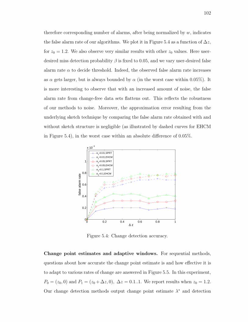
102
therefore corresponding number of alarms, after being normalized by w, indicates
the false alarm rate of our algorithms. We plot it in Figure 5.4 as a function of ∆z,
for z0 = 1.2. We also observe very similar results with other z0 values. Here user-
desired miss detection probability β is fixed to 0.05, and we vary user-desired false
alarm rate α to decide threshold. Indeed, the observed false alarm rate increases
as α gets larger, but is always bounded by α (in the worst case within 0.05%). It
is more interesting to observe that with an increased amount of noise, the false
alarm rate from change-free data sets flattens out. This reflects the robustness
of our methods to noise. Moreover, the approximation error resulting from the
underlying sketch technique by comparing the false alarm rate obtained with and
without sketch structure is negligible (as illustrated by dashed curves for EHCM
in Figure 5.4), in the worst case within an absolute difference of 0.05%.
0 0.2 0.4 0.6 0.8 10
0.2
0.4
0.6
0.8
1
x 10−3
∆ z
fals
e al
arm
rat
e
α1=0.01,SPRT
α1=0.01,EHCM
α2=0.05,SPRT
α2=0.05,EHCM
α3=0.1,SPRT
α3=0.1,EHCM
Figure 5.4: Change detection accuracy.
Change point estimates and adaptive windows. For sequential methods,
questions about how accurate the change point estimate is and how effective it is
to adapt to various rates of change are answered in Figure 5.5. In this experiment,
P0 = (z0, 0) and P1 = (z0 +∆z, 0), ∆z = 0.1..1. We report results when z0 = 1.2.
Our change detection methods output change point estimate λ∗ and detection
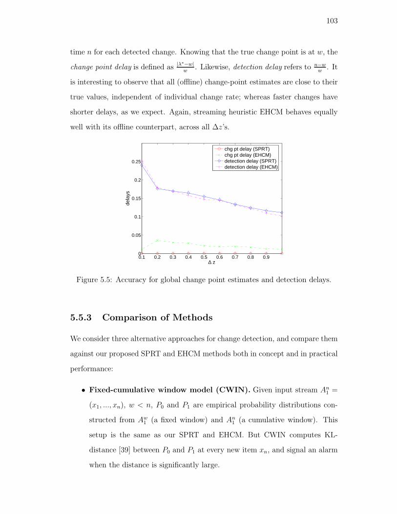
103
time n for each detected change. Knowing that the true change point is at w, the
change point delay is defined as |λ∗−w|w
. Likewise, detection delay refers to n−ww
. It
is interesting to observe that all (offline) change-point estimates are close to their
true values, independent of individual change rate; whereas faster changes have
shorter delays, as we expect. Again, streaming heuristic EHCM behaves equally
well with its offline counterpart, across all ∆z’s.
0.1 0.2 0.3 0.4 0.5 0.6 0.7 0.8 0.90
0.05
0.1
0.15
0.2
0.25
∆ z
dela
ys
chg pt delay (SPRT)chg pt delay (EHCM)detection delay (SPRT)detection delay (EHCM)
Figure 5.5: Accuracy for global change point estimates and detection delays.
5.5.3 Comparison of Methods
We consider three alternative approaches for change detection, and compare them
against our proposed SPRT and EHCM methods both in concept and in practical
performance:
• Fixed-cumulative window model (CWIN). Given input stream An1 =
(x1, ..., xn), w < n, P0 and P1 are empirical probability distributions con-
structed from Aw1 (a fixed window) and An
1 (a cumulative window). This
setup is the same as our SPRT and EHCM. But CWIN computes KL-
distance [39] between P0 and P1 at every new item xn, and signal an alarm
when the distance is significantly large.

104
• Fixed-sliding window model (FSWIN). This algorithm has a similar
flavor to CWIN, but differs in the way that P1 is built based on the most
recent w observations Ann−w+1 = (xn−w+1 . . . xn), which forms a sliding win-
dow of size w.
• Benchmark Sequential Method (BSM). Different from our algorithms,
BSM assumes that not only P0 but also P1 is known as a priori, so that it
guarantees optimum in terms of detection delay [109].
Detection delay. We compare them against our SPRT and EHCM. Again in
this experiment, P0 = (z0, 0)), P1 = (z0 + ∆z, 0), ∆z = 0.1..1, and the true
change point is at w. Without knowing the true threshold to trigger significant
changes with window-based methods (i.e., CWIN and FSWIN), we adopt a con-
servative threshold — the KL-distance between distributions (z0, 0) and (z0, 1).
This is smaller than the true threshold, since we consider it change-free by adding
random noise N(0, 1) to the original data. So the detection delay using the con-
servative threshold is shorter than the true delay. We compare it against detection
delays from other methods, and infer the comparative results when using the true
threshold.
All methods start detecting changes since xw+1. Figure 5.6 demonstrates the
results when z0 = 1.2. As expected, the detection delay of each method decreases
with the increase of ∆z. CWIN yields the longest detection delay, and even
misses detections in the first three streams when change is small. This is because
points prior to the change point decay the amount of change in distribution.
Therefore FSWIN performs better, since it forgets all stale data that arrive at
least w time steps ago. And we can infer that delays from a change detection
algorithm with decaying-weighted window will fall between those from FSWIN
and CWIN. However, FSWIN’s detection delay is still roughly twice of the delay
from equally-well-performed SPRT and EHCM. This indicates the effectiveness
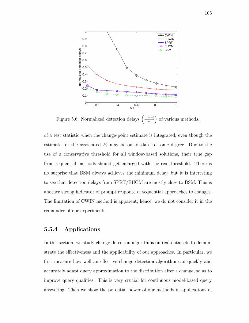
105
0.2 0.4 0.6 0.8 10
0.1
0.2
0.3
0.4
0.5
0.6
0.7
0.8
0.9
1
∆ z
norm
aliz
ed d
etec
tion
dela
ys
CWINFSWINSPRTEHCMBSM
Figure 5.6: Normalized detection delays(
|n−w|w
)
of various methods.
of a test statistic when the change-point estimate is integrated, even though the
estimate for the associated P1 may be out-of-date to some degree. Due to the
use of a conservative threshold for all window-based solutions, their true gap
from sequential methods should get enlarged with the real threshold. There is
no surprise that BSM always achieves the minimum delay, but it is interesting
to see that detection delays from SPRT/EHCM are mostly close to BSM. This is
another strong indicator of prompt response of sequential approaches to changes.
The limitation of CWIN method is apparent; hence, we do not consider it in the
remainder of our experiments.
5.5.4 Applications
In this section, we study change detection algorithms on real data sets to demon-
strate the effectiveness and the applicability of our approaches. In particular, we
first measure how well an effective change detection algorithm can quickly and
accurately adapt query approximation to the distribution after a change, so as to
improve query qualities. This is very crucial for continuous model-based query
answering. Then we show the potential power of our methods in applications of

106
intrusion detection.
Query quality. We obtain the world cup ’98 HTTP request logs from the
Internet Traffic Archive [76]. We take hourly requests from one server, and focus
on the ClientID attribute contained in each HTTP request record. Analyzing
the data offline finds that logs usually present different distributions in ClientID
across time. We concatenate two one-hour log files S0 = (x1 . . . xw) and S1 =
(xw+1 . . . xn) for our experiments; w + 1 is the true change point. We have about
9K distinct ClientID in this data set, on which we compare FSWIN and EHCM
via a set of queries. Our goal for each query is to quickly and accurately answer
it according to the post-change distribution, when it occurs. The ground truth
is query results Q answered from S1. For each change detection algorithm to be
compared, we first run it on the concatenated data set, with P0 being the empirical
distribution constructed from S0, to get a change-point estimate λ, from which we
start to estimate query answers Q based on all observations after λ. In particular,
λ output from EHCM is an estimate for the most likely change point, whereas
FSWIN with a window of size w returns λ = n−w + 1 if a change is detected at
time n.
Here are the set of queries [96] and the criteria we use to evaluate the accuracy
of various query answers (U is a data domain of size u):
• Point queries: let P2 and P2 be empirical probability distributions con-
structed from respective S1 and (xλ . . . xn), where λ is the change-point
estimate returned from a change detection algorithm, and P2 is an estimate
for P2. A point query Q(i) is to return an approximation of P2[i]. Thus,
the accuracy of point-query estimates is 1− 1u
∑
i∈U|Q(i)−Q(i)|
Q(i);
• φ-quantiles (0 < φ < 1): let F (x) =∑
i∈U ,i≤xP2[i]. The j-th φ-quantile
Q(j) is to find x, such that F (x − 1) < jφ, F (x) ≥ jφ, 1 ≤ j ≤ 1/φ.
Likewise, Q(j) is an estimate for Q(j) when P2 is replaced by P2. So the
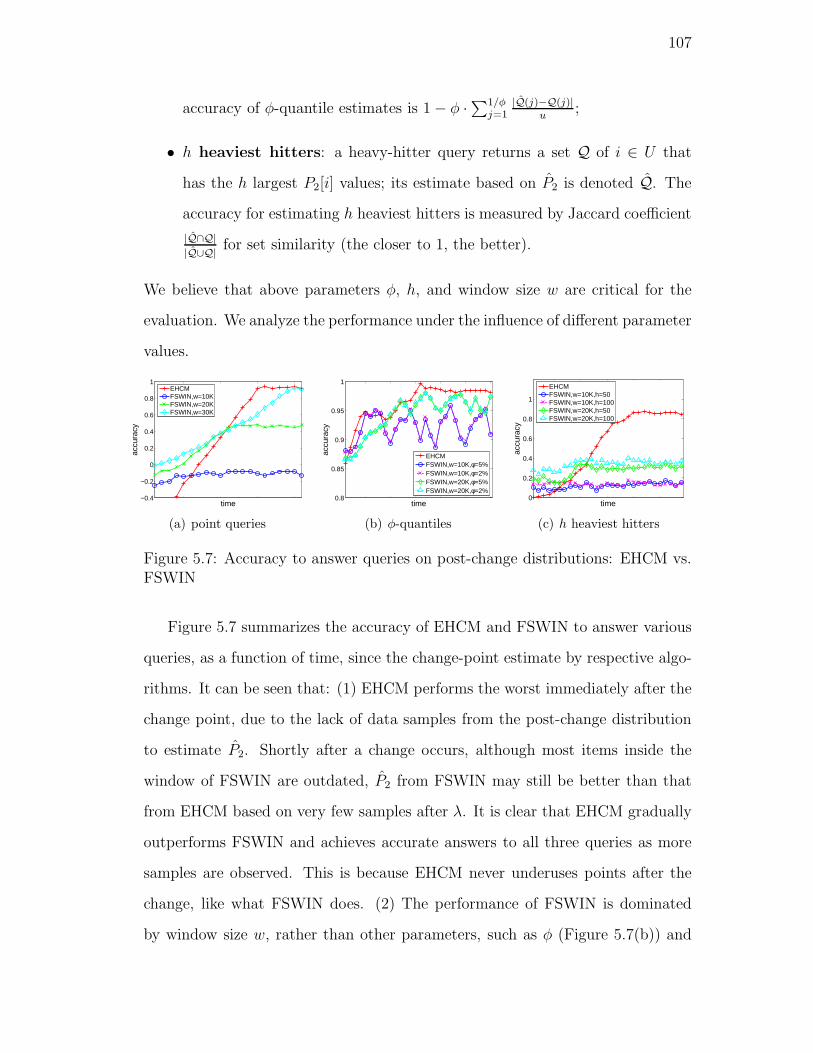
107
accuracy of φ-quantile estimates is 1− φ ·∑1/φj=1
|Q(j)−Q(j)|u
;
• h heaviest hitters: a heavy-hitter query returns a set Q of i ∈ U that
has the h largest P2[i] values; its estimate based on P2 is denoted Q. The
accuracy for estimating h heaviest hitters is measured by Jaccard coefficient
|Q∩Q|
|Q∪Q|for set similarity (the closer to 1, the better).
We believe that above parameters φ, h, and window size w are critical for the
evaluation. We analyze the performance under the influence of different parameter
values.
−0.4
−0.2
0
0.2
0.4
0.6
0.8
1
time
accu
racy
EHCMFSWIN,w=10KFSWIN,w=20KFSWIN,w=30K
(a) point queries
0.8
0.85
0.9
0.95
1
time
accu
racy
EHCMFSWIN,w=10K,φ=5%FSWIN,w=10K,φ=2%FSWIN,w=20K,φ=5%FSWIN,w=20K,φ=2%
(b) φ-quantiles
0
0.2
0.4
0.6
0.8
1
time
accu
racy
EHCMFSWIN,w=10K,h=50FSWIN,w=10K,h=100FSWIN,w=20K,h=50FSWIN,w=20K,h=100
(c) h heaviest hitters
Figure 5.7: Accuracy to answer queries on post-change distributions: EHCM vs.FSWIN
Figure 5.7 summarizes the accuracy of EHCM and FSWIN to answer various
queries, as a function of time, since the change-point estimate by respective algo-
rithms. It can be seen that: (1) EHCM performs the worst immediately after the
change point, due to the lack of data samples from the post-change distribution
to estimate P2. Shortly after a change occurs, although most items inside the
window of FSWIN are outdated, P2 from FSWIN may still be better than that
from EHCM based on very few samples after λ. It is clear that EHCM gradually
outperforms FSWIN and achieves accurate answers to all three queries as more
samples are observed. This is because EHCM never underuses points after the
change, like what FSWIN does. (2) The performance of FSWIN is dominated
by window size w, rather than other parameters, such as φ (Figure 5.7(b)) and

108
h (Figure 5.7(c)): smaller windows (relative to the domain size) lead to inaccu-
rate approximation results, whereas too large windows delay the convergence to
accurate answers (see w = 30K in Figure 5.7(a)), since it takes longer for larger
windows to “forget” all stale data. All these make EHCM the method of choice.
This suggests the importance of accurate change-point estimate in model-based
declarative query answering.
5.6 Local Change Detection Experiments
We evaluate in this section the efficacy of our proposed method SPRT and its
streaming heuristic that we dub EHCM (Section 5.4) for detecting local changes.
We set up experiments with synthetic data as in Section 5.5.1.
Accuracy of Detected Local Changes. We verify the effectiveness of our
methods to recognize significant local changes based on prior knowledge on dis-
tributions. To avoid enumerating all possible changes, we consider two repre-
sentative types of changes: type I, small-to-medium changes, in particular from
P0 = (1.2, 0) to P1 = (1.3, 0); type II, medium-to-large changes, in particular
from P0 = (1.2, 0) to P1 = (1.7, 0). In both cases, the ground truth is that the
set Gk contains singleton items j ∈ U where top-k local Kullback-Leibler (KL)
distance values dKL(P1[j]||P0[j]) = P1[j] log(P1[j]/P0[j]) achieve. Figure 5.8(a)
shows the top-100 local KL distance values. With this ground truth, we shall
evaluate the accuracy of local changes triggered by our local change detection
algorithms. Conceptually, all local changes in j should be signaled when its lo-
cal distance is greater than some threshold. However, this empirical threshold
for local KL distance values is not pre-computable, so we propose the evaluation
procedure as follows.
Zipf distributions have a property that relatively large local changes happen
at the head of a distribution, when switching from P0 to P1. Therefore, a given
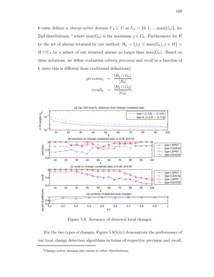
109
k-value defines a change-active domain Uk ⊂ U as Uk = {0, 1, ..., max(Gk)}, for
Zipf distributions, 1 where max(Gk) is the maximum j ∈ Gk. Furthermore, let H
be the set of alarms returned by our method; Hk = {j|j ≤ max(Gk), j ∈ H} =
H ∩ Uk be a subset of our returned alarms no larger than max(Gk). Based on
these notations, we define evaluation criteria precision and recall as a function of
k (note this is different from traditional definitions):
precisonk =|Hk ∩Gk||Hk|
,
recallk =|Hk ∩Gk||Gk|
.
10 20 30 40 50 60 70 80 90 10010
−4
10−2
k
k−th
larg
est d
KL
(a) top−100 local KL distances from change−contained data
type I: (1.2,0) → (1.3,0)type II: (1.2,0) → (1.7,0)
10 20 30 40 50 60 70 80 90 1000.8
0.9
1
k
prec
isio
n
(b) precision on change−contained data, α=0.05, β=0.05
type I,SPRTtype II,EHCMtype I,SPRTtype II,EHCM
10 20 30 40 50 60 70 80 90 1000.6
0.8
1
k
reca
ll
(c) recall on change−contained data, α=0.05, β=0.05
type I,SPRTtype II,EHCMtype I,SPRTtype II,EHCM
0.1 0.2 0.3 0.4 0.5 0.6 0.7 0.8 0.9 10.60.8
1
∆ zJaca
rd C
oeffi
cien
ts
(d) similarity of detected local changes
Figure 5.8: Accuracy of detected local changes.
For the two types of changes, Figure 5.8(b)(c) demonstrate the performance of
our local change detection algorithms in terms of respective precision and recall,
1Change-active domain also exists in other distributions.

110
when false alarm rate α = 0.05, miss detection rate β = 0.05. It is clear to see
that precision and recall from detecting medium-to-large (type II) changes are
both higher than those from detecting small-to-medium (type I) changes. This
is consistent with our intuition that it is easier to detect larger changes. When
focusing on either type of changes, precision increases with k increasing, with
the worse case value of 85%, and converges to higher than 95% at large k (as
α = 0.05 indicates). This suggests Hk become stable (i.e., no more alarms output
from our algorithm), while Gk keeps expanding. In contrast, recall starts high
(very close to 1) and collapses after some k (i.e., k = 35 in type I, k = 70 in type
II). This indicates that local changes out of these top-k are no longer significant
to signal alarms, although they have relatively high ranking in Figure 5.8(a). All
these constitute a potential indicator of our accurate and robust change detection
algorithms. Moreover, it is interesting to observe that the type I and type II
curves in Figure 5.8(a) have very close y-value at k = 35 and k = 70, respec-
tively, as shown by the horizontal line, which suggests an empirical threshold to
significant local changes, under KL distance. We next factor in the additional
error resulting from our streaming heuristic EHCM. Figure 5.8(b)(c) show that
our streaming algorithm for local change detection performs equally well with its
offline counterpart.
Furthermore, we apply both offline and streaming algorithms for detecting
local changes to 10 change-contained streams; each has 100K points, the first
and the second w = 50K points of which are generated from P0 = (1.2, 0), P1 =
(1.2 + ∆z, 0), respectively, ∆z = 0.1..1, in increments of 0.1. We compute, for
each stream, the similarity between the set of detected local changes by respective
SPRT and EHCM. The measurement we use is the Jaccard coefficient [41]. High
Jaccard-coefficient values, as shown in Figure 5.8(d), indicate the accuracy of our
streaming algorithm.
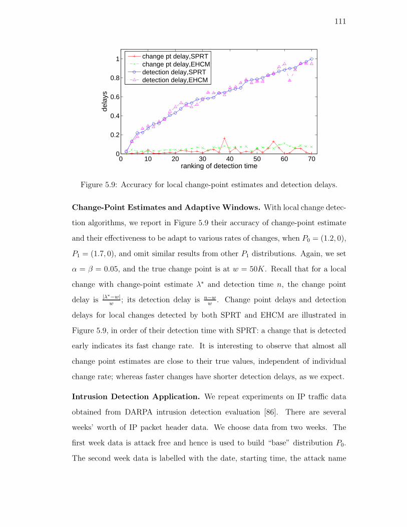
111
0 10 20 30 40 50 60 700
0.2
0.4
0.6
0.8
1
ranking of detection time
dela
ys
change pt delay,SPRTchange pt delay,EHCMdetection delay,SPRTdetection delay,EHCM
Figure 5.9: Accuracy for local change-point estimates and detection delays.
Change-Point Estimates and Adaptive Windows. With local change detec-
tion algorithms, we report in Figure 5.9 their accuracy of change-point estimate
and their effectiveness to be adapt to various rates of changes, when P0 = (1.2, 0),
P1 = (1.7, 0), and omit similar results from other P1 distributions. Again, we set
α = β = 0.05, and the true change point is at w = 50K. Recall that for a local
change with change-point estimate λ∗ and detection time n, the change point
delay is |λ∗−w|w
; its detection delay is n−ww
. Change point delays and detection
delays for local changes detected by both SPRT and EHCM are illustrated in
Figure 5.9, in order of their detection time with SPRT: a change that is detected
early indicates its fast change rate. It is interesting to observe that almost all
change point estimates are close to their true values, independent of individual
change rate; whereas faster changes have shorter detection delays, as we expect.
Intrusion Detection Application. We repeat experiments on IP traffic data
obtained from DARPA intrusion detection evaluation [86]. There are several
weeks’ worth of IP packet header data. We choose data from two weeks. The
first week data is attack free and hence is used to build “base” distribution P0.
The second week data is labelled with the date, starting time, the attack name

112
and the target destination IP addresses of each attack. 2 We pair up two data
sets from the same day of each week, and start our EHCM algorithm to check for
any deviation of the second week data from the first.
We focus on two types of attacks that occurred during the day: ‘setan’ —
a network probing attack which looks for well-known weaknesses; and ‘neptune’
— SYN flood denial of service on one or more ports. Both attacks lead to an
increase in packet number in network traffic, so that the distribution of overall
packet traffic shifts towards these IP addresses during the attacks. From labelled
header data, the ground truth is:
Attack names Target IP Starting time
setan 172.16.114.50 9:33 AM
neptune 172.16.114.207 11:04 AM
When packet count distribution is considered, EHCM detects above attacks
at 9:33:32 AM and 11:05:44 AM, with change point estimates being 9:33:32AM
and 11:05:27 AM, respectively. This suggests that our proposed method has the
potential for intrusion detection monitoring. However, if we apply EHCM to
traffic volume (i.e., in terms of number of bytes) distribution, the attack ‘setan’ is
not detected. This indicates that different signals demonstrate different behavior
with respect to the changing distribution. Better understanding of how attacks
entail changes in underlying distributions is needed to apply sequential change
detection to intrusion detection applications.
5.7 Related Work
There is a lot of work on change detection in data streams. Most [54, 80, 39, 31, 84]
are based on fixed-size windows: they affix two windows to streaming data and
estimate the change in distribution between them. A delay in change detection
2Note the difference between changes and attacks. An attack may result in (global or local)changes in distributions; whereas changes may not result from attacks.

113
is inevitable when the time-scale of change is unavailable. Authors in [54, 80, 39]
exploited parallel windows of different sizes to adapt to different change scales.
But this is not suitable in data stream context, since we can not afford to explore
all window sizes. On the other hand, it has been proposed to use windows of
varied sizes [53, 111, 13]. This line of research has to guess a priori the time-scale
of change, and is mostly computationally expensive. Ho [71] recently proposed
a martingale framework for change detection on data streams, where a “pseudo-
adaptive” window – delimited by two adjacent change detection points – was used.
However, no change point estimate was considered in this work. In contrast to
the bulk of this literature, our approaches differ in two key ways. First, when
a change is detected, our methods also estimate the most likely change point in
time. Second, the change-point estimate is inherent to the evaluation of our test
statistic to detect a change, hence, our methods achieve shorter detection delays.
Applying sequential hypothesis testing to change detection is a natural ap-
proach. Authors in [79] studied sequential change detection method offline, under
a simpler scenario: (1) both pre- and post-change distributions are known as a
priori; (2) the first observation is assumed to be the change point. Our work here
is more general, being able to estimate the actual change point anywhere which
is the crux of the problem. In addition, our challenge is to adapt the well-known
technique to the streaming scenario, even without independence assumption. An-
other relevant work is [19], where they adopted exponential histograms to detect
change of various scales. However, their approach does not work for data with
large domain size, which is our crucial focus.
For local change detection, [31, 84] proposed window-based solutions to find
relatively large local changes. However, they triggered a large local change at a
singleton item when its difference is at least a user-specified fraction of the sum
of differences of all items. This may not indicate a change in the underlying
distribution, since the total difference may be small. In contrast, we extend

114
sequential probability ratio test to both offline and streaming algorithms to detect
statistically significant local changes.
5.8 Chapter Summary
There has been plenty of work on techniques for detecting changes in data, but
most, if not all, focus on certain “windows” to define and study changes in dis-
tributions. This is limiting since window size is a parameter that needs to be
determined which is nontrivial, and its size is a lower bound on the detection
delay. We have adopted the sound statistical method of sequential hypothesis
testing to yield fast and space-efficient algorithms on streams, to detect both
global and local changes, without explicit window specification. Our methods
are oblivious to data’s underlying distributions, and work without independence
assumption. Our detailed study of these methods in practice with synthetic and
real data sets reveals their effectiveness in detecting changes and many insights
on their applicability and their use, depending on the nature of change in the
distribution these phenomena induce.

115
Chapter 6
Conclusions and Future Work
Nowadays, many organizations have applications that deal with millions or even
billions of transactions every day. Under this scenario, a lot of work on designing
techniques for processing and mining such streaming data has emerged in the
past decade. Prior work in streaming analysis has shown how to estimate simple
statistics such as frequent items, quantiles, histograms, join sizes etc. on data
streams, but very little has focused on more sophisticated statistical analyses that
are performed in near real-time, using limited resources. We present streaming
techniques for such statistical modeling in this dissertation.
In our study, we investigate two representative categories of modeling in data
streams: parametric and structural modeling.
For parametric modeling, there are hierarchical as well as non-hierarchical
models. We present highly efficient, small-space approaches for estimating re-
spective model parameters. To the best of our knowledge, this is the first work
on model fitting over data streams with a priori error guarantees. In addition,
we propose online method for model validation so that models can be validated
frequently.
For structural modeling, we focus on communication graphs. With the abun-
dance of communication between individuals, many applications on analyzing the
patterns behind the communications emerge. The idea of using signatures to cap-
ture behavior is an attractive one. Instead of proposing a signature scheme for
a particular task, we take a systematic way to study the principles behind the

116
usage of signatures to any task. In particular, we define fundamental properties
of signatures and study a broad set of applications based on what properties they
need for signatures to be useful. We explore several signature schemes in our
framework and evaluate them on real data in terms of these properties. This
provides insights into suitable signature schemes for desired applications. Our
experiments demonstrate that no single signature scheme fits all applications;
different signatures are needed, depending on the balance among the properties
they provide.
Another critical issue in modeling data streams is to detect its change. There
has been plenty of work on detecting changes in streams, but most, if not all, focus
on certain “windows” to detect the change in distribution between them. This is
problematic since window size is a parameter that needs to be determined which
is nontrivial. We therefore adopt statistically sound sequential probability ratio
test to yield fast and space-efficient streaming algorithm to detect both global and
local changes, without explicit window specification. Our methods are oblivious to
data’s underlying distributions, and work without the independence assumption.
Another advantage of our proposed sequential approaches is shorter detection
delays. This is due to the integration of most likely change-point estimate into
the test statistics of our solutions.
As concrete applications of our techniques, we focus on network traffic data,
one of the richest sources for data streams. We complement our analytic and
algorithmic results with experiments on them to demonstrate the practicality
of our methods at line speeds, and potential power of streaming techniques for
statistical modeling in data mining.
In future work, we propose to study the following.
• Parametric modeling: widely used general modeling procedures that involve
recursive computing such as expectation maximization, as well as regression
models other than linear regression presented in this dissertation, will be

117
explored.
• Structural modeling: we will consider the temporal dimension on signatures
in communication graphs. Interesting questions include but are not limited
to “What is the signature at a given time interval?”, “What sequence of ac-
tivities capture my communication behavior?”, etc. Another line of research
is to study hierarchies of signatures over time. Furthermore, advanced hash-
ing is a promising technique to speed up nearest-neighbor searches among
signatures.
• Change detection: Almost all real world data sets are beyond single dimen-
sion, so we shall address the problems with higher dimensions in our future
work.

118
Bibliography
[1] STREAM: Stanford stream data manager, http://www-
db.stanford.edu/stream/.
[2] Sprint CMON, http://www.sprintlabs.com/.
[3] http://www.streambase.com/.
[4] D. Abadi, D. Carney, U. Cetintemel, M. Cherniack, C. Convey, C. Erwin,
E. Galvez, M. Hatoun, A. Maskey, A. Rasin, A. Singer, M. Stonebraker,
N. Tatbul, Y. Xing, R. Yan, and S. Zdonik. Aurora: a data stream man-
agement system. In SIGMOD, 2003.
[5] L. Adamic. Zipf, power-law, pareto - a ranking tutorial. http://www.hpl.
hp.com/research/idl/papers/ranking/, 2000.
[6] N. Alon, N. Duffield, C. Lund, and M. Thorup. Estimating sums of arbitrary
selections with few probes. In ACM PODS, pages 317–325, 2005.
[7] N. Alon, Y. Matias, and M. Szegedy. The space complexity of approximating
the frequency moments. JCSS, 58:137–147, 1999.
[8] A. Arasu and G. S. Manku. Approximate counts and quantiles over sliding
windows. In PODS, 2004.
[9] B. Babcock, S. Babu, M. Datar, R. Motwani, and J. Widom. Models and
issues in data stream systems. In PODS, 2002.

119
[10] Ziv Bar-Yossef. Sampling lower bounds via information theory. In STOC
’03: Proceedings of the thirty-fifth annual ACM symposium on Theory of
computing, pages 335–344, 2003.
[11] Ziv Bar-Yossef, T. S. Jayram, Ravi Kumar, D. Sivakumar, and Luca Tre-
visan. Counting distinct elements in a data stream. In RANDOM ’02:
Proceedings of the 6th International Workshop on Randomization and Ap-
proximation Techniques, pages 1–10, London, UK, 2002. Springer-Verlag.
[12] P. Barford, A. Bestavros, A. Bradley, and M. Crovella. Changes in web
client access patterns characteristics and caching implications. In WWW,
1999.
[13] P.L. Bartlett, S. Ben-David, and S.R. Kulkarni. Learning changing concepts
by exploiting the structure of change. In Computational Learing Theory,
pages 131–139, 1996.
[14] M. Basseville and I.V. Nikiforov. Detection of Abrupt Changes: Theory and
Application. Prentice-Hall, Inc.
[15] J. Baumes, M. Goldberg, M. Hayvanovych, M. Magdon-Ismail, W.A. Wal-
lace, and M. Javeed Zaki. Finding hidden group structure in a stream of
communications. In ISI, 2006.
[16] A. Belussi and C. Faloutsos. Estimating the selectivity of spatial queries
using the ‘correlation’ fractal dimension. In VLDB, 1995.
[17] P. Berkhin. A survey on pagerank computing. Internet Mathematics,
2(1):73–120, 2005.
[18] Z. Bi, C. Faloutsos, and F. Korn. The ”dgx” distribution for mining massive,
skewed data. In KDD, 2001.
120
[19] A. Bifet and R. Gavalda. Learning from time-changing data with adaptive
windowing. In SDM, 2007.
[20] A. Chakrabarti, K. Do Ba, and S. Muthukrishnan. Estimating entropy and
entropy norm on data streams. In STACS, pages 196–205, 2006.
[21] A. Chakrabarti, G. Cormode, and A. McGregor. A near-optimal algorithm
for computing the entropy of a stream. In Proceedings of ACM-SIAM Sym-
posium on Discrete Algorithms, pages 328–335, 2007.
[22] Kaushik Chakrabarti, Minos Garofalakis, Rajeev Rastogi, and Kyuseok
Shim. Approximate query processing using wavelets. The VLDB Journal,
10(2-3):199–223, 2001.
[23] S. Chandrasekaran, O. Cooper, A. Deshpande, M.J. Franklin, J.M. Heller-
stein, W. Hong, S. Krishnamurthy, S.R. Madden, F. Reiss, and M.A. Shah.
TelegraphCQ: continuous dataflow processing. In SIGMOD, 2003.
[24] M. Charikar, K. Chen, and M. Farach-Colton. Finding frequent items in
data streams. In ICALP, 2002.
[25] C.-M. Chen, H. Agrawal, M. Cochinwala, and D. Rosenbluth. Stream query
processing for healthcare bio-sensor applications. In ICDE, 2004.
[26] CIDR, http://www.webopedia.com/TERM/C/CIDR.html.
[27] E. Cohen and M. Strauss. Maintaining time-decaying stream aggregates.
In PODS, 2003.
[28] D. Coppersmith and R. Kumar. An improved data stream algorithm for
frequency moments. In SODA, 2004.
[29] G. Cormode, T. Johnson, F. Korn, S. Muthukrishnan, O. Spatscheck, and
D. Srivastava. Holistic udafs at streaming speeds. In SIGMOD, 2004.
121
[30] G. Cormode and S. Muthukrishnan. An improved data stream summary:
The count-min sketch and its applications. In LATIN, 2004.
[31] G. Cormode and S. Muthukrishnan. What is new: Finding significant dif-
ferences in network data streams. In INFOCOM, pages 1534–1545, 2004.
[32] G. Cormode and S. Muthukrishnan. Summarizing and mining skewed data
streams. In SDM, 2005.
[33] G. Cormode, S. Muthukrishnan, and I. Rozenbaum. Summarizing and min-
ing inverse distributions on data streams via dynamic inverse sampling. In
VLDB, 2005.
[34] Graham Cormode, Mayur Datar, Piotr Indyk, and S. Muthukrishnan. Com-
paring data streams using hamming norms (how to zero in). IEEE Trans-
actions on Knowledge and Data Engineering, 15(3):529–540, 2003.
[35] C. Cortes and D. Pregibon. Signature-based methods for data streams.
Data Min. Knowl. Discov., 5(3):167–182, 2001.
[36] Corinna Cortes, Daryl Pregibon, and Chris Volinsky. Communities of in-
terest. Lecture Notes in Computer Science, 2189, 2001.
[37] C. D. Cranor, T. Johnson, O. Spatscheck, and V. Shkapenyuk. Gigascope:
A stream database for network applications. In SIGMOD, 2003.
[38] Chuck Cranor, Yuan Gao, Theodore Johnson, Vlaidslav Shkapenyuk, and
Oliver Spatscheck. Gigascope: high performance network monitoring with
an sql interface. In SIGMOD ’02: Proceedings of the 2002 ACM SIGMOD
international conference on Management of data, pages 623–623, 2002.
[39] T. Dasu, S. Krishnan, S. Venkatasubramanian, and K. Yi. An information-
theoretic approach to detecting changes in multi-dimensional data streams.
In Interface, 2006.
122
[40] M. Datar, A. Gionis, P. Indyk, and R. Motwani. Maintaining stream statis-
tics over sliding windows. In SODA, 2002.
[41] M. Datar and S. Muthukrishnan. Estimating rarity and similarity over data
stream windows. In ESA, 2002.
[42] A. Deshpande, C. Guestrin, and S. Madden. Using probabilistic models for
data management in acquisitional environments. In CIDR, 2005.
[43] A. Deshpande, C. Guestrin, S. Madden, J.M. Hellerstein, and W. Hong.
Model-driven data acquisition in sensor networks. In VLDB, 2004.
[44] A. Deshpande, C. Guestrin, S. Madden, J.M. Hellerstein, and W. Hong.
Model-based approximate querying in sensor networks. VLDB Journal,
2005.
[45] M. Evans, N. Hastings, and B. Peacock. Statistical Distributions. Wiley,
New York, 3rd edition, 2000.
[46] C. Faloutsos and I. Kamel. Beyond uniformity and independence: Analysis
of R- trees using the concept of fractal dimension. In PODS, 1994.
[47] C. Faloutsos, Y. Matias, and A. Silberschatz. Modeling skewed distributions
using multifractals and the ’80-20 law’. In VLDB, 1996.
[48] T. Fawcett and F.J. Provost. Activity monitoring: Noticing interesting
changes in behavior. In SIGKDD, 1999.
[49] Joan Feigenbaum, Sampath Kannan, Andrew McGregor, Siddharth Suri,
and Jian Zhang. Graph distances in the streaming model: the value of space.
In SODA ’05: Proceedings of the sixteenth annual ACM-SIAM symposium
on Discrete algorithms, pages 745–754, Philadelphia, PA, USA, 2005. Soci-
ety for Industrial and Applied Mathematics.
123
[50] Joan Feigenbaum, Sampath Kannan, Andrew McGregor, Siddharth Suri,
and Jian Zhang. On graph problems in a semi-streaming model. Theor.
Comput. Sci., 348(2):207–216, 2005.
[51] P. Flajolet and G.N. Martin. Probabilistic counting. In FOCS, 1983.
[52] X. Gabaix, P. Gopikrishnan, V. Plerou, and H.E. Stanley. A theory of power
law distributions in financial market fluctuations. 423:267–270, 2003.
[53] J. Gama, P. Medas, G. Castillo, and P. Rodrigues. Learning with drift
detection. In Lecture Notes in Computer Science, 2004.
[54] V. Ganti, J.E. Gehrke, R. Ramakrishnan, and W.-Y. Loh. A framework
for measuring changes in data characteristics. Journal of Computer and
System Sciences, 64:542–578, 2002.
[55] J. Gehrke, F. Korn, and D. Srivastava. On computing correlated aggregates
over continual data streams. In SIGMOD, 2001.
[56] P.B. Gibbons. Distinct sampling for highly-accurate answers to distinct
values queries and event reports. In VLDB, 2001.
[57] P.B. Gibbons and Y. Matias. Synopsis data structures for massive data
sets. In DIMACS Series in Discrete Mathematics and Theoretical Computer
Science: Special Issue on External Memory Algorithms and Visualization,
volume A, 1999.
[58] Phillip B. Gibbons and Srikanta Tirthapura. Estimating simple functions
on the union of data streams. In ACM Symposium on Parallel Algorithms
and Architectures, pages 281–291, 2001.
[59] D. Gibson, R. Kumar, and A. Tomkins. Discovering large dense subgraphs
in massive graphs. In VLDB, 2005.

124
[60] A.C. Gilbert, S. Guha, P. Indyk, Y. Kotidis, S. Muthukrishnan, and
M. Strauss. Fast, small-space algorithms for approximate histogram main-
tenance. In STOC, pages 389–398, 2002.
[61] A.C. Gilbert, W. Willinger, and A. Feldmann. Scaling analysis of conser-
vative cascades, with applications to network traffic. In IEEE Transaction
on Information Theory, volume 45, pages 971–991, 1999.
[62] T. Krishnan G.J. McLachlan. The EM Algorithm and Extensions. Wiley-
Interscience, 1996.
[63] M. Greenwald and S. Khanna. Space-efficient online computation of quantile
summaries. In SIGMOD, 2001.
[64] Sudipto Guha. Space efficiency in synopsis construction algorithms. In
VLDB ’05: Proceedings of the 31st international conference on Very large
data bases, pages 409–420, 2005.
[65] Sudipto Guha, Nick Koudas, and Kyuseok Shim. Data-streams and his-
tograms. In ACM Symposium on Theory of Computing, pages 471–475,
2001.
[66] Sudipto Guha, Andrew McGregor, and Suresh Venkatasubramanian.
Streaming and sublinear approximation of entropy and information dis-
tances. In SODA ’06: Proceedings of the seventeenth annual ACM-SIAM
symposium on Discrete algorithm, pages 733–742, 2006.
[67] Taher H. Haveliwala. Topic-sensitive pagerank. In WWW, 2002.
[68] S. Hill, D. Agarwal, R. Bell, and C. Volinsky. Building an effective rep-
resentation for dynamic network. Computational and Graphical Statistics,
15(3):584–608(25), 2006.
125
[69] S. Hill and F. Provost. The myth of the double-blind review? Author
identification using only citations. SIGKDD Explorations, 5(2):179–184,
2003.
[70] S. Hill, F. Provost, and C. Volinsky. Network-based marketing: Identifying
likely adopters via consumer networks. Statistical Science, 21(2):256–276,
2006.
[71] S. Ho. A martingale framework for concept change detection in time-varying
data streams. In ICML, pages 321–327, 2005.
[72] G. Hulten, L. Spencer, and P. Domingos. Mining time-changing data
streams. In SIGKDD, 2001.
[73] A. Hussain, J. Heidemann, and C. Papadopoulos. Identification of repeated
dos attacks. In INFOCOM, 2006.
[74] P. Indyk. Stable distributions, pseudorandom generators, embeddings and
data stream computation. In FOCS, pages 189–197, 2000.
[75] P. Indyk and R. Motwani. Approximate nearest neighbors: towards remov-
ing the curse of dimensionality. In STOC, 1998.
[76] Internet traffic archive. http://ita.ee.lbl.gov.
[77] A.K. Jain, R.W. Duin, and J. Mao. Statistical pattern recognition: A
review. IEEE Transaction on Pattern Analysis and Machine Intelligence,
22(1):4–37, 2000.
[78] C. Jr, A. Traina, L. Wu, and C. Faloutsos. Fast feature selection using the
fractal dimension. In SBBD, 2000.
[79] J. Jung, V. Paxson, A.W. Berger, and H. Balakrishnan. Fast portscan de-
tection using sequential hypothesis testing. In IEEE symposium on security
and privacy, 2004.
126
[80] D. Kifer, S. Ben-David, and J. Gehrke. Detecting changes in data streams.
In VLDB, 2004.
[81] E. Kohler, J. Li, V. Paxson, and S. Shenker. Observed structure of addresses
in ip traffic. In IMC, 2002.
[82] F. Korn, S. Muthukrishnan, and Y. Wu. Modeling skew in data streams.
In SIGMOD, 2006.
[83] B. Krishnamurthy, H. Madhyastha, and O. Spatscheck. ATMEN: a trig-
gered network measurement infrastructure. In WWW, 2005.
[84] B. Krishnamurthy, S. Sen, Y. Zhang, and Y. Chen. Sketch-based change
detection: methods, evaluation, and applications. In IMC, 2003.
[85] A. Lakhina, M. Crovella, and C. Diot. Diagnosing network-wide traffic
anomalies. In SIGCOMM, 2004.
[86] DARPA intrusion detection evaluation. http://www.ll.mit.edu/IST/
ideval/index.html.
[87] F. Li, C. Chang, G. Kollios, and A. Bestavros. Characterizing and exploiting
reference locality in data stream applications. In ICDE, 2006.
[88] T. Liu, C.M. Sadler, P. Zhang, and M. Martonosi. Implementing software on
resource-constrained mobile sensors: Experiences with impala and zebranet.
In MobiSys, 2004.
[89] D. Madigan. DIMACS working group on monitoring message streams.
http://http://stat.rutgrs.edu/∼madigan/mms/.
[90] B.B. Mandelbrot. Fractals and Scaling in Finance. Springer-Verlag, New
York, 1997.
127
[91] G. S. Manku and R. Motwani. Approximate frequency counts over data
streams. In VLDB, 2002.
[92] Gurmeet Singh Manku, Sridhar Rajagopalan, and Bruce G. Lindsay. Ran-
dom sampling techniques for space efficient online computation of order
statistics of large datasets. In SIGMOD ’99: Proceedings of the 1999 ACM
SIGMOD international conference on Management of data, pages 251–262,
1999.
[93] S.J. Mason and N.E. Graham. Areas beneath the relative operating char-
acteristics (ROC) and relative operating levels (ROL) curves: Statistical
significance and interpretation. Q. J. R. Meteorol. Soc, 30:291–303, 1982.
[94] MassDAL poster. http://www.cs.rutgers.edu/∼muthu/massdalposter.
pdf.
[95] R. Motwani and P. Raqhavan. Randomized Algorithms. Cambridge Univer-
sity Press, 1995.
[96] S. Muthukrishnan. Data streams: Algorithms and applications. Founda-
tions and Trends in Theoretical Computer Science, 1(2), 2005.
[97] Cisco netflow. http://www.cisco.com/warp/public/cc/pd/iosw/ioft/
neflct/tech/napps wp.htm.
[98] J. Newsome, B. Karp, and D. Song. Polygraph: Automatically generating
signatures for polymorphic worms. In Symposium on Security and Privacy,
2005.
[99] C.C. Noble and D.J. Cook. Graph-based anomaly detection. In SIGKDD,
2003.
[100] B.-U. Pagel, F. Korn, and C. Faloutsos. Deflating the dimensionality curse
using multiple fractal dimensions. In ICDE, 2000.

128
[101] S. Papadimitriou, H. Kitagawa, P. B. Gibbons, and C. Faloutsos. Loci: Fast
outlier detection using the local correlation integral. In ICDE, 2003.
[102] S.I. Resnick. Heavy tail modeling and teletraffic data. The Annals of Statis-
tics, 25:1805–1869, 1997.
[103] M. Roughan and C. Kalmanek. Pragmatic modeling of broadband access
traffic. In Computer Communications 26(8), 2003.
[104] M. Schroeder. Fractals, Chaos, Power Laws: Minutes From an Infinite
Paradise. W.H. Freeman and Company, New York, 1991.
[105] Nisheeth Shrivastava, Chiranjeeb Buragohain, Divyakant Agrawal, and
Subhash Suri. Medians and beyond: new aggregation techniques for sensor
networks. In SenSys ’04: Proceedings of the 2nd international conference
on Embedded networked sensor systems, pages 239–249, 2004.
[106] D. Song, P. Venable, and A. Perrig. User recognition by keystroke latency
pattern analysis. 1997.
[107] J. Sun, H. Qu, D. Chakrabarti, and C. Faloutsos. Relevance search and
anomaly detection in bipartite graphs. SIGKDD Explorations Special Issue
on Link Mining, 7(2):48–55, 2005.
[108] Chayant Tantipathananandh, Tanya Berger-Wolf, and David Kempe. A
framework for community identification in dynamic social networks. In
KDD ’07: Proceedings of the 13th ACM SIGKDD international conference
on Knowledge discovery and data mining, pages 717–726, 2007.
[109] A. Wald. Sequential Analysis. Dover Publications, 2004.
[110] M. Wang, T. Madhyastha, N.H. Chan, S. Papadimitriou, and C. Faloutsos.
Data mining meets performance evaluation: Fast algorithm for modeling
bursty traffic. In ICDE, 2002.
129
[111] G. Widmer and M. Kubat. Learning in the presence of concept drift and
hidden contexts. Machine Learning, 23(1):69–101, 1996.
[112] W. Willinger, D. Alderson, and L. Li. A pragmatic approach to dealing
with high-variability in network measurements. In IMC, 2004.
[113] W. Willinger and V. Paxson. Where mathematics meets the internet. No-
tices of the American Mathematical Society, 45(8):961–970, 1998.
[114] W. Willinger, V. Paxson, and M.S. Taqqu. Self-similarity and Heavy Tails:
Structural Modeling of Network Traffic. Chapman & Hall, New York, 1998.
[115] A. Wong, L. Wu, P.B. Gibbons, and C. Faloutsos. Fast estimation of fractal
dimension and correlation integral on stream data. In Inf. Process. Lett.
93(2): 91-97, 2005.
[116] Eugene Wu, Yanlei Diao, and Shariq Rizvi. High-performance complex
event processing over streams. In SIGMOD ’06: Proceedings of the 2006
ACM SIGMOD international conference on Management of data, pages
407–418, 2006.
[117] K. Xu, Z. Zhang, and S. Bhattacharyya. Profiling internet backbone traffic:
behavior models and applications. SIGCOMM Comput. Commun. Rev.,
35(4):169–180, 2005.
[118] Y. Yao and J. Gehrke. Query processing in sensor networks. In CIDR, 2003.
[119] Y. Zhu and D. Shasha. Statstream: Statistical monitoring of thousands of
data streams in real time. In VLDB, pages 358–369, 2002.

130
Curriculum Vita
Yihua Wu
EDUCATION
October 2007 Ph.D. in Computer Science, Rutgers University, U.S.A.
May 2003 M.S. in Computer Science, Rutgers University, U.S.A.
July 2000 B.S. in Computer Science, Peking University, Beijing, P.R. China
EXPERIENCE
Jan.2007—Aug.2007 Research Assistant, Department of Computer Sci-ence, Rutgers University, New Brunswick, NJ
Oct.2004—Sep.2007 Research Consultant, Database Management Re-search Department, AT&T Shannon Research Lab, Florham Park, NJ
Jan.2006—Dec.2006 Teaching Assistant, Department of Computer Sci-ence, Rutgers University, New Brunswick, NJ
Jan.2005—Dec.2005 Research Assistant, Department of Computer Sci-ence, Rutgers University, New Brunswick, NJ
Sep.2001—Dec.2004 Teaching Assistant, Department of Computer Sci-ence, Rutgers University, New Brunswick, NJ
Jan.2001—Apr.2001 Software Engineer, Asia Electronic Commerce Ltd.,Beijing, P.R. China
PUBLICATION
On Signatures for Communication Graphs. Graham Cormode, Flip Korn,S. Muthukrishnan and Yihua Wu. Submitted.
Sequential Change Detection on Data Streams. S. Muthukrishnan, Ericvan den Berg and Yihua Wu. In International Conference on Data Mining(ICDM) Workshop on Data Stream Mining and Management, 2007.

131
Modeling Skew in Data Streams. Flip Korn, S. Muthukrishnan and YihuaWu. In Proceedings of the 2006 ACM SIGMOD International Conferenceon Management of Data (SIGMOD), 2006.
Fractal Modeling of IP Network Traffic at Streaming Speeds. Flip Korn, S.Muthukrishnan and Yihua Wu. In Proceedings of the 22nd IEEE Conferenceon Data Engineering (ICDE), 2006.