Portland State University Portland State University

PDXScholar PDXScholar

Dissertations and Theses Dissertations and Theses

Summer 1-1-2012

Streamflow Analysis and a Comparison of Streamflow Analysis and a Comparison of

Hydrologic Metrics in Urban Streams Hydrologic Metrics in Urban Streams

Matthew Lawton Wood Portland State University

Follow this and additional works at: https://pdxscholar.library.pdx.edu/open_access_etds

Part of the Nature and Society Relations Commons, Physical and Environmental Geography

Commons, and the Urban Studies and Planning Commons

Let us know how access to this document benefits you.

Recommended Citation Recommended Citation Wood, Matthew Lawton, "Streamflow Analysis and a Comparison of Hydrologic Metrics in Urban Streams" (2012). Dissertations and Theses. Paper 769. https://doi.org/10.15760/etd.769

This Thesis is brought to you for free and open access. It has been accepted for inclusion in Dissertations and Theses by an authorized administrator of PDXScholar. Please contact us if we can make this document more accessible: pdxscholar@pdx.edu.

Streamflow Analysis and a Comparison of Hydrologic Metrics in Urban Streams

by

Matthew Lawton Wood

A thesis submitted in partial fulfillment of the requirements for the degree of

Master of Science in

Geography

Thesis Committee: Heejun Chang, Chair

Martin Lafrenz Joseph Poracsky

Portland State University ©2012

i

Abstract

This study investigates the hydrologic effects of urbanization in two Portland,

Oregon streams through a comparison of three hydrologic metrics. Hydrologic metrics

used in this study are the mean annual runoff ratio (Qa), mean seasonal runoff ratio (Qw

and Qd), and the fraction of time that streamflow exceeds the mean streamflow during the

year (TQmean). Additionally, the relative change in streamflow in response to storm

events was examined for two watersheds. For this investigation urban development is

represented by two urbanization metrics: percent impervious and road density.

Descriptive and inferential statistics were used to evaluate the relationship between the

hydrologic metrics and the amount of urban development in each watershed. The effect

of watershed size was also investigated using nested watersheds, with watershed size

ranging from 6 km2 to 138km2. The results indicate that annual and seasonal runoff ratios

have difficulty capturing the dynamic hydrologic behavior in urban watersheds. TQmean

was useful at capturing the flashy behavior of the Upper Fanno watershed, however it did

not perform as well in Kelley watershed possibly due to the influence of impermeable

soils and steep slopes. Unexpected values for hydrologic metrics in Lower Johnson,

Sycamore and Kelley watersheds could be the result water collection systems that appear

to route surface water outside of their watersheds as well as permeable soils. Storm event

analysis was effective at characterizing the behavior for the selected watersheds,

indicating that shorter time scales may best capture the dynamic behavior of urban

watersheds.

ii

Acknowledgements I would like express my gratitude to all of those who without this thesis would not have

been possible. I would like to acknowledge the indispensible advice and guidance of my

advisor Dr. Heejun Chang. I also thank the members of my committee, Joseph Poracsky

and Martin Lafrenz for their guidance and suggestions. I am grateful to Il-won Jung for

his technical expertise assisting with data manipulation. I would like to thank my fiancée

Gabriela for her endless support and encouragement throughout this process. Lastly,

thanks to my family who have always encouraged me to pursue my interests and dreams.

iii

Table of Contents Abstract ................................................................................................................................ i

Acknowledgements ............................................................................................................. ii

List of Tables ..................................................................................................................... iv

List of Figures ......................................................................................................................v

I. Introduction ..............................................................................................................1

II. Study Area ...............................................................................................................7

III. Data and Methods ..................................................................................................11

IV. Results ....................................................................................................................17

V. Discussion ..............................................................................................................21

VI. Conclusions ............................................................................................................29

VII. References ..............................................................................................................47

iv

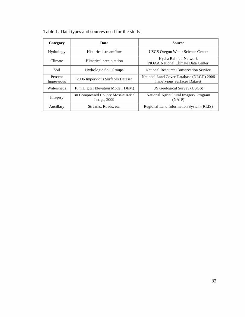
List of Tables Table 1. Data types and sources used for the study ...........................................................32

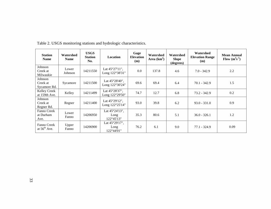
Table 2. USGS monitoring stations and hydrologic characteristics ..................................33

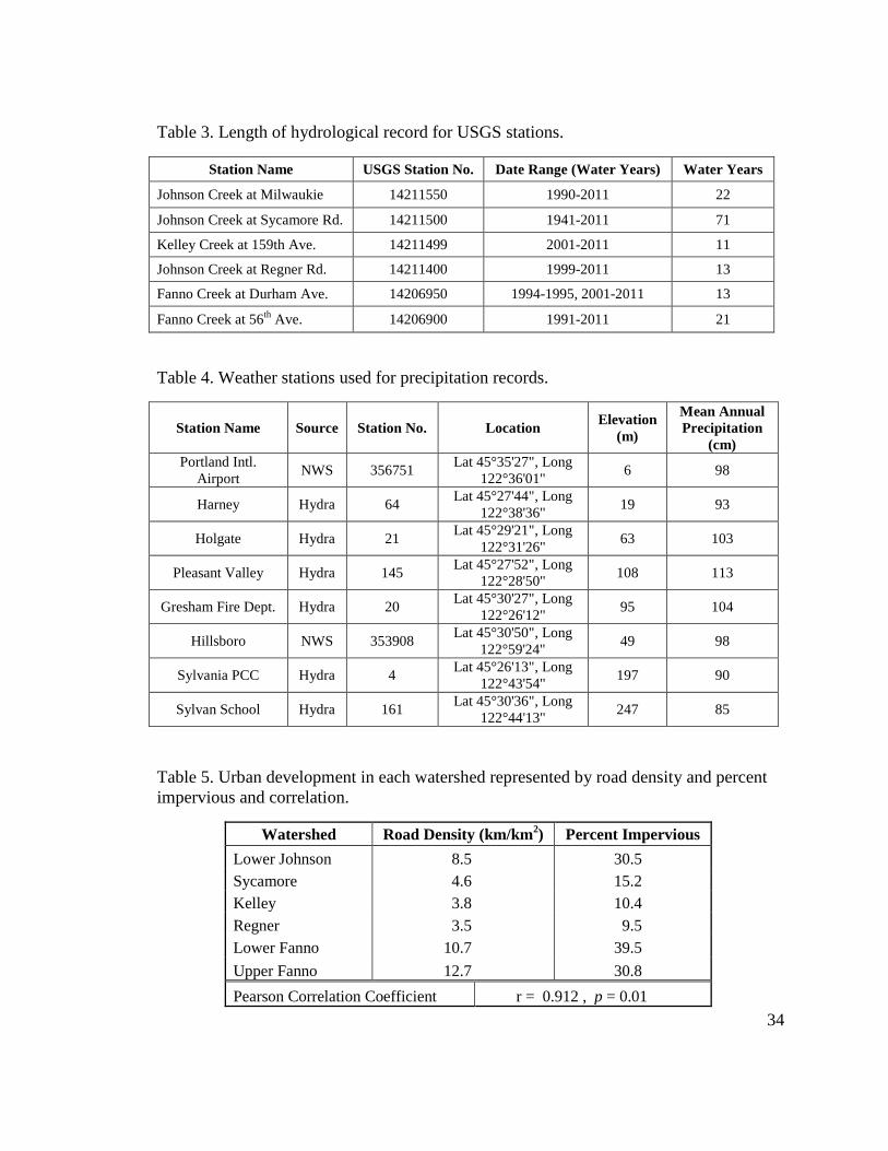
Table 3. Length of hydrological record for USGS stations ...............................................34

Table 4. Weather stations used for precipitation records ...................................................34

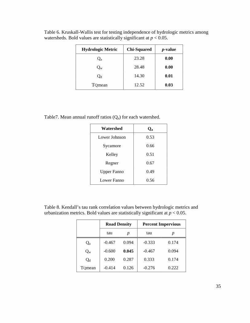
Table 5. Urban development in each watershed represented by road density and percent impervious and correlation ................................................................................................34 Table 6. Kruskall-Wallis test for testing independence of hydrologic metrics among watersheds. Bold values are statistically significant at p < 0.05 ....................................... 35 Table 7. Mean annual runoff ratios (Qa) for each watershed .............................................35

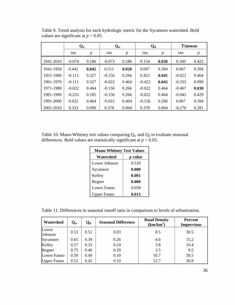
Table 8. Kendall’s tau rank correlation values between hydrologic metrics and urbanization metrics. Bold values are statistically significant at p < 0.05 .........................35 Table 9. Trend analysis for each hydrologic metric for the Sycamore watershed. Bold values are significant at p < 0.05 .......................................................................................36 Table 10. Mann-Whitney test values comparing Qw and Qd to evaluate seasonal differences. Bold values are statistically significant at p < 0.05 ........................................36 Table 11. Differences in seasonal runoff ratio in comparison to levels of urbanization ...36

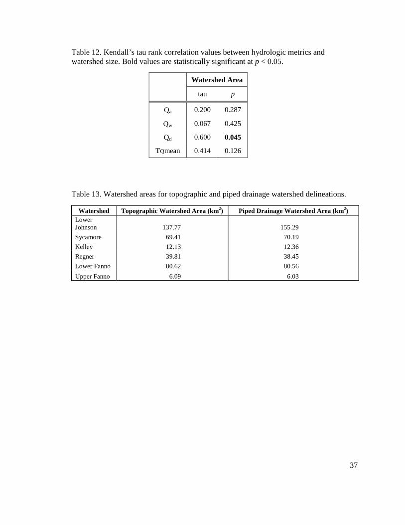
Table 12. Kendall’s tau rank correlation values between hydrologic metrics and watershed size. Bold values are statistically significant at p < 0.05 ..................................37 Table 13. Watershed areas for topographic and piped drainage watershed delineations ..37

v

List of Figures Figure 1. Map of Fanno and Johnson Creek watersheds study area and subwatersheds ...38 Figure 2. Relationship between elevation and annual mean precipitation for Johnson Creek Hydra rain gages used to adjust Portland International Airport NWS Station ........38 Figure 3. Map of Fanno and Johnson Creek “piped drainage watershed” delineated using both the topology and stormwater sewer network .............................................................39 Figure 4. Distribution of mean annual runoff ratios (Qa) for 2001-2011 ..........................39 Figure 5. Relationship between mean annual runoff ratio (Qa) and percent impervious ...40 Figure 6. Relationship between mean annual runoff ratio (Qa) and road density ..............40 Figure 7. Distribution of mean seasonal runoff ratios (Qw, Wet Season and Qd, Dry Season) for 2001-2011 .......................................................................................................41 Figure 8. Relationship between road density and the wet season runoff ratio (Qw) ..........41 Figure 9. Relationship between percent impervious and the wet season runoff ratio (Qw) ............................................................................................................................42 Figure 10. Distribution of fraction of time that daily mean flow exceeds annual mean flow (TQmean) for 2001-2011 ............................................................................................42 Figure 11. Relationship between TQmean and road density ..............................................43 Figure 12. Relationship between TQmean and percent impervious ...................................43 Figure 13. Effects of precipitation on changes in streamflow for Lower Fanno watershed ...........................................................................................................................44 Figure 14. Effects of precipitation on changes in streamflow for the Lower Johnson watershed ...........................................................................................................................44 Figure 15. Watershed geology ...........................................................................................45 Figure 16. Watershed soil types .........................................................................................45 Figure 17. Watershed slope in degrees ..............................................................................46 Figure 18. Relationship between USGS gage elevation and mean annual runoff ratio (Qa) ............................................................................................................................46

1

I. Introduction

With more than 80% of the U.S. population and nearly half of the world’s

population living in urban areas in 2007, urbanization of landscapes is pervasive and

growing rapidly (United Nations 2008). National comparisons display that the state of

Oregon has experienced above average population growth, with an annual average rate of

1.2% from 2000 to 2006. Much of the growth has been within urban areas, with 78% of

Oregon’s population residing in one of six metropolitan statistical areas (Oregon

Population Report 2009). Oregon’s largest city, Portland, has experienced rapid

population growth reflected by a 19% increase from 1980 to 1990, a 21% increase from

1990 to 2000 and a 10.3% increase from 2000 to 2010 (US Census Bureau 2012). As

populations continue to grow, conversion of land from rural to urban will continue and

urbanization will place pressure upon regional water resources (United Nations 2008).

Urbanization is a global phenomenon that is dramatically altering the natural

hydrologic processes and is directly and indirectly impairing the health of the world’s

water systems. The conversion of permeable surfaces into impervious urban structures is

accompanied by the following major changes in nearby streams: increased contribution

and decreased transport time of surface runoff; reduced lag time between precipitation

event and peak flow event; a decreased contribution of precipitation into the groundwater

system; increased peak flows and decreased low flows.

Urban development alters the hydrologic cycle by removing vegetation and

replacing pervious land with impervious surfaces such as buildings and roads. Impervious

surfaces associated with urban development prevent the infiltration of rainfall into

groundwater systems, and instead leads to increased surface runoff. Stormwater drainage

2

systems associated with urban development further alter the natural hydrologic cycle by

routing surface runoff into underground drainage pipes and into nearby streams. These

changes result in faster conveyance of precipitation events into streams, and the effects

have been well documented. The objectives of this study are to investigate the

performance of hydrologic metrics utilized to characterize the behavior of urban streams.

Changes in land use and land cover have been shown to directly affect a system’s

water yield by altering the hydrologic cycle (Chang 2007). The principal effects of urban

development are changes in peak flow characteristics, total runoff volume, and water

quality (Leopold 1968; Hammer 1972; Paul and Meyer 2001). The modification of land

surface during urban development exposes soil to storm runoff, yielding high sediment

loads in streams (Leopold 1968). Increased imperviousness has been associated with

increases in urban runoff, evapotranspiration, and nonpoint source pollution (Bhaduri et

al. 2001). Increases in urban runoff have been shown to increase the frequency and

magnitude of flood events (Booth and Jackson 1997).

A variety of physical characteristics determine watershed response to

precipitation events. Watershed land use and land cover have been widely used as

predictors of stream behavior and health. In addition to climate patterns, soil type, land

cover, and elevation, the amount of impervious surface has emerged as a useful indicator

of land development and its effect on watershed health (Schueler 1994; Arnold and

Gibbons 1996). The use of impervious cover as a predictor of watershed and stream

health has demonstrated the effects of urban areas on surface runoff (Horner et al. 1997),

baseflow (Kauffman et al. 2009), streamflow (Hollis 1975; Jennings and Jarnagin 2002),

3

channel incision (Leopold 1956; Hardison et al. 2009), water quality (May et al. 1997),

and aquatic habitat and life (Finkenbine et al. 2000; Ourso and Frenzel 2003).

Arnold and Gibbons (1996) cited the usefulness of imperviousness as an

environmental indicator due to two factors. First, imperviousness is integrative in its

ability to predict cumulative water resource impacts without regard to specific factors

(e.g. water quality, hydrology, biotic integrity). Second, it is measurable in that there are

a variety of techniques used to measure imperviousness. Importantly, impervious cover is

not measured or characterized in the same way by all researchers. Common methods

include total impervious area (TIA), percent impervious, effective impervious area (EIA),

curve numbers (CN) and urban intensity indices (e.g. road density).

A great deal of research has investigated the link between the presence of

impervious cover with changes in stream health and behavior. Cianfrani et al. (2006)

surveyed forty-six independent stream reaches in south eastern Pennsylvania and using

multivariate statistical analysis found a significant relationship, linking higher TIA values

with reduced large woody debris and channel sinuosity. Finkenbine et al. (2000) found

that increases in TIA were correlated with a decrease in summer baseflow, and a decrease

of instream cover available for aquatic life. Schiff and Benoit (2007) used a

multiparameter water quality index in a New Haven, Connecticut watershed and found a

critical level of 5% TIA, above which stream quality declined. Research conducted in the

Pacific Northwest however, has suggested a threshold for urban stream health at 10%

imperviousness (Booth 1991).

In an evaluation of urban streamflow patterns in the Puget Lowland of

Washington, Konrad et al. (2005) utilized both %TIA and road density to represent the

4

level of urban development within their study area. Their investigation found road

density was significantly correlated with reference high flow events and not reference

flows based on cumulative runoff volume or the duration of the flow. This correlation

indicates that urban development increases the frequency of high flows but not their

cumulative duration. It has been shown that cumulative streamflow volume, often

represented by mean streamflow rate Qmean, does not always change in response to

urbanization (Rose and Peters 2001; Konrad and Booth 2002; Konrad et al. 2005).

In the same study Konrad et al. (2005) used three hydrologic metrics to

investigate the influence of urban development on stream channel form and streambed

stability. The hydrologic metrics they selected, fraction of time streamflow exceeds mean

streamflow (TQmean), the coefficient of variation of annual maximum streamflow

(CVAMF), and the fraction of time streamflow exceeds the 0.5-year flood (T0.5), integrated

the “storm-scale effects” of urban development on annual to decadal scale. TQmean was

shown to significantly decline in two creeks where extensive urban development had

occurred in the watershed, and displayed weaker relationships in other creeks which had

much lower rates of urbanization.

DeGasperi et al. (2009) investigated the relationship between fifteen hydrologic

metrics, urban land cover, and the Benthic Index of Biological Integrity (B-IBI) in the

Puget Lowland, Washington. Eight hydrologic metrics were significantly correlated with

B-IBI scores and all but two hydrologic metrics were significantly correlated with the

urbanization metrics, TIA and urban land cover. Their results suggest that the biological

integrity of streams is significantly impacted by the hydrology of urbanized watersheds.

5

Interestingly, TQmean was one of the two hydrologic metrics that was not significantly

correlated with the measures of urbanization.

Streamflow characteristics of watersheds with varying levels of urbanization were

evaluated by Rose and Peters (2001) in the Atlanta, Georgia area. Their evaluation of

streamflow using various hydrologic metrics found that the most urbanized watershed

displayed peak flows 30 to 100% greater and low-flows 25 to 35% less than those in less

urbanized streams. These results are consistent with the effects of urbanization as

impervious surfaces reduce hydraulic transport time creating faster and greater peak

flows, and preventing infiltration of precipitation into the groundwater, thereby reducing

groundwater contributions to low flows.

While the impact of the urban built environment on hydrologic systems has been

widely researched, each system is uniquely influenced by its climate, soils, geology,

impervious surfaces, and provides the opportunity to apply hydrologic analysis

techniques in new ways. This research utilizes documented techniques including,

hydrologic metrics, urbanization metrics and storm event analysis, and applies them a

variety of nested scales. The use of nested scales in watershed analysis has been

suggested as one way to detect hydrologic impacts of urbanization (Jones 1997), but has

not been utilized within Johnson and Fanno Creek watersheds. The large amount of

hydrologic data in each watershed provides the opportunity to reveal new insights

regarding each system.

This research presents a comparison of hydrologic metrics that seek to quantify

the effects of urban development. A comparison of these metrics among watersheds with

various levels of development will demonstrate the relationship between increased

6

development and hydrologic response. Comparison of two urbanization metrics will also

demonstrate any difference in quantifying the amount of development within a watershed

and its effect upon surface hydrology. Additionally, the use of watersheds varying in size,

as well as a nested watershed approach, will examine any relationship between watershed

size and metric performance.

The purposes of this study are to: 1) Evaluate the hydrologic response to

urbanization in two streams by use of hydrologic metrics, 2) Evaluate any correlation

between the hydrologic metrics and urbanization metrics for each watershed 3) Compare

hydrologic metrics at different spatial sizes using nested subwatersheds.

7

II. Study Area

The City of Portland is the largest city in the state of Oregon with an estimated

population of 583,776, incorporated in three counties (US Census Bureau, 2010).

Portland experienced significant growth through much of the 1980s and 1990s, and while

population growth has slowed within the city, the neighboring suburbs of Hillsboro and

Beaverton continue to experience rapid population growth (US Census Bureau 2009).

Due to the pressures of population growth, surrounding rural areas will increasingly be

under the pressures of urban development. As urban development continues, more

pervious green spaces will be converted to impervious surfaces and impact the

surrounding hydrologic regime.

This research will focus on two watersheds, Fanno and Johnson Creek, located

within the Portland metropolitan area of Oregon. These watersheds were chosen because

both have been impacted by urbanization, but they differ in their land use and drainage

basin characteristics. Additionally, there is a large amount of hydrological data available

from multiple stations within each watershed allowing for different size drainage areas to

be evaluated. Johnson Creek flows 41 km from its head waters in Boring, Oregon,

through Clackamas and Multnomah Counties to its confluence with the Willamette River

in Milwaukie, Oregon. The upper reaches of Johnson Creek flow west from agricultural

lands, through residential and commercial/industrial areas of Gresham and Portland. The

lower reach of the creek is highly urbanized and surrounded by dense residential and

commercial/industrial areas.

Crystal Springs, Sunshine Creek, Butler Creek, Hogan Creek, Badger Creek, and

Kelley Creek are the major tributaries that contribute streamflow to Johnson Creek.

8

Crystal Springs is a series of springs that discharge into the Crystal Springs Creek

flowing 4km west from Reed College then south through Westmoreland Park and finally

feeding into Johnson Creek. There are numerous other small tributaries which also feed

into Johnson Creek, most of which are located south of the creek. Kelley Creek is a 7 km

long tributary of Johnson Creek located just east of Portland that has primarily consisted

of forest and agriculture, but in recent years has witnessed increased urban land

development. The 2002 inclusion of Kelley Creek within the Portland metropolitan

urban growth boundary (UGB) is sure to facilitate housing and commercial growth

(Metro 2012). The Kelley Creek watershed provides an excellent opportunity to evaluate

pre-urbanization hydrologic conditions. Previous research has shown that Kelly Creek is

sensitive to altered discharge patterns that accompany increases in impervious surfaces

and preserving headwater forests could protect it from disruption (Levell and Chang

2008; Murphy 2009).

Fanno Creek is a 24 km tributary of the Tualatin River that flows south from its

headwaters near the Tualatin Hills in southwest Portland through the cities of Beaverton,

Tigard and Durham. The 80 km2 Fanno Creek watershed is highly urbanized and has seen

most of its land converted to buildings, roads, streets and other impervious surfaces. The

watershed contains steep slopes in areas and consists of primarily silt loam soils. There

are a number of smaller tributaries that drain in to Fanno Creek, including Woods Creek,

Ash Creek and Vermont Creek.

Differences in the amount of urbanization and physical characteristics such as

watershed slope and soil characteristics, result in different hydrological processes and

provide an opportunity for investigation. Selection of the watersheds for this study was

9

based on the following criteria: at least a ten-year period of recorded hourly streamflow;

at least ten-years of hourly precipitation data from a nearby weather station; and no

ponds, diversions or dams that would significantly alter the streamflow. Johnson and

Fanno Creeks met those criteria, serving as ideal cases for this investigation.

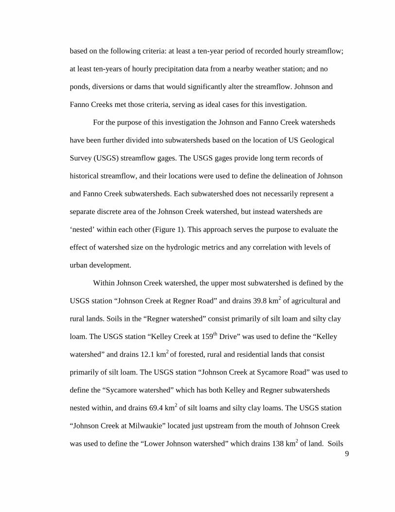
For the purpose of this investigation the Johnson and Fanno Creek watersheds

have been further divided into subwatersheds based on the location of US Geological

Survey (USGS) streamflow gages. The USGS gages provide long term records of

historical streamflow, and their locations were used to define the delineation of Johnson

and Fanno Creek subwatersheds. Each subwatershed does not necessarily represent a

separate discrete area of the Johnson Creek watershed, but instead watersheds are

‘nested’ within each other (Figure 1). This approach serves the purpose to evaluate the

effect of watershed size on the hydrologic metrics and any correlation with levels of

urban development.

Within Johnson Creek watershed, the upper most subwatershed is defined by the

USGS station “Johnson Creek at Regner Road” and drains 39.8 km2 of agricultural and

rural lands. Soils in the “Regner watershed” consist primarily of silt loam and silty clay

loam. The USGS station “Kelley Creek at 159th Drive” was used to define the “Kelley

watershed” and drains 12.1 km2 of forested, rural and residential lands that consist

primarily of silt loam. The USGS station “Johnson Creek at Sycamore Road” was used to

define the “Sycamore watershed” which has both Kelley and Regner subwatersheds

nested within, and drains 69.4 km2 of silt loams and silty clay loams. The USGS station

“Johnson Creek at Milwaukie” located just upstream from the mouth of Johnson Creek

was used to define the “Lower Johnson watershed” which drains 138 km2 of land. Soils

10

within the Lower Johnson watershed consist primarily of silt loams and urban complex

soils that have been mixed, manipulated and disturbed.

The Fanno Creek watershed contains two USGS stations with long term

hydrological records, resulting in one nested watershed in the upper reach. The USGS

station “Fanno at 56th Avenue” was used to delineate the “Upper Fanno watershed”, and

drains 6.1 km2 of highly developed land and as a result consists almost entirely of urban

complex soils. The USGS station “Fanno at Durham Avenue” was used to delineate the

“Lower Fanno watershed” and drains 80.6 km2 of silt loam and urban complex soils.

The City of Portland operates and maintains the combined sewer system (CSS),

municipal stormwater sewer system and underground injection control (UIC) systems

within the urban areas of Portland. The CSS collects both sewage and stormwater runoff

in a single pipe for 33 km2 east of the Willamette, much of which falls in the Lower

Johnson watershed (City of Portland, 2010). The stormwater sewer system drains 63 km2

of land for the entire Portland region. As of 2008, it was estimated that there are 11,000

publicly owned UICs and 25,000 to 35,000 privately owned UICs in the Portland

metropolitan area (Snyder 2008). The City of Portland’s stormwater management

infrastructure alters the natural drainage characteristics of both Fanno and Johnson Creek

watersheds and while they are not directly included in this study, their role and impact is

considered while interpreting the results of this analysis.

11

III. Data and Methods

3.1 Data

Daily streamflow data from U.S. Geological Survey (USGS) monitoring stations

was acquired for each watershed (Table 1). Six USGS streamflow monitoring stations,

four in Johnson Creek and two in Fanno Creek, were used for daily streamflow data and

their locations were used to delineate subwatersheds (Table 2). The USGS stations have

different lengths of hydrological records with Johnson at Sycamore having the longest

record of 70 years and Kelley the shortest record of 10 years (Table 3). The long term

records available for the Sycamore station allow for temporal analysis to be conducted in

this study.

Daily precipitation data was acquired from the City of Portland Hydra Rainfall

Network and the National Weather Service (Table 1). The Hydra Rainfall Network

consists of 36 rain gages within the Portland metropolitan area and has collected hourly

rainfall data at stations beginning in 1998. Hydra stations that were closest to USGS

stations and provided complete historical records were used for this study. Six Hydra rain

gages, four in Johnson Creek and two in Fanno Creek, provided daily precipitation data

(Table 4). For precipitation records prior to available Hydra records, historical

precipitation data was obtained from NWS stations in Hillsboro and at the Portland

International Airport (Table 4). The Hillsboro NWS station was for the Lower and Upper

Fanno watersheds, while the Portland International Airport (PDX) NWS Station was used

for the Lower Johnson, Sycamore, Kelley and Regner watersheds.

The data used for percent impervious was acquired from the USGS Seamless Data

Warehouse. The 2006 National Land Cover Database (NLCD) Impervious Surface

12

dataset for the conterminous United States is a 30-meter resolution raster file representing

the percent impervious on the ground. Each 30 x 30 raster cell has a unique value ranging

from 0-100 representing the percentage of impervious cover. The impervious raster file

was clipped using the boundaries of each watershed in the study. The resulting raster files

were used to obtain an average value that represented the percent of impervious cover for

each watershed.

A 10-meter Digital Elevation Model (DEM) from the USGS National Elevation

Dataset was acquired for watershed delineation. Previously delineated watershed

boundaries that incorporated the influence of the Metro area’s stormwater drainage

network were also acquired for anecdotal comparisons with topographic delineations.

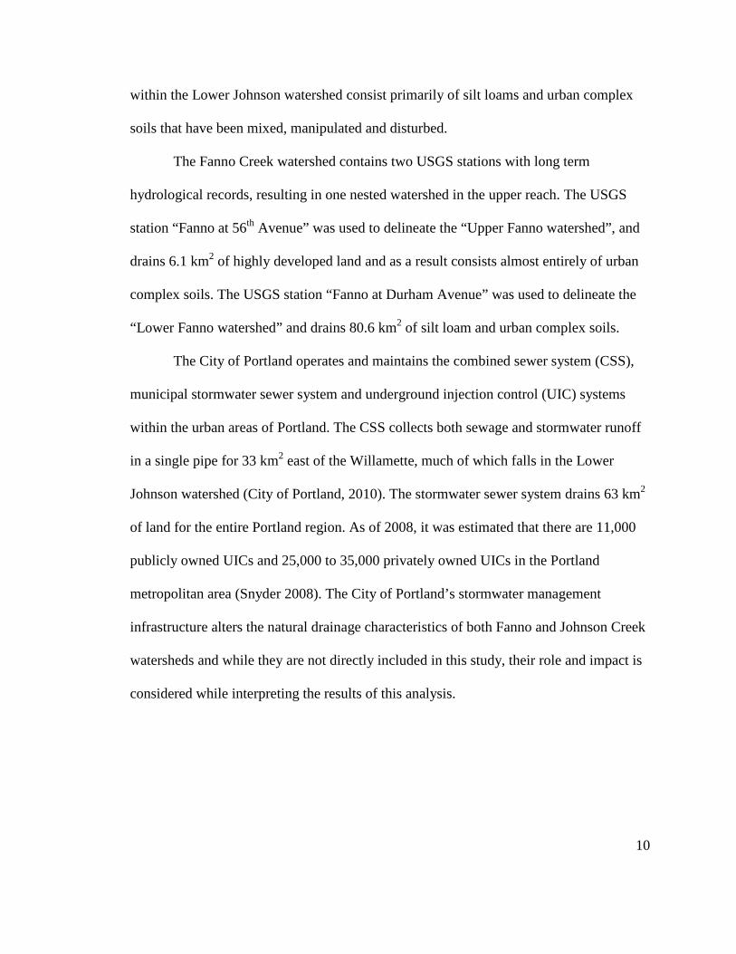
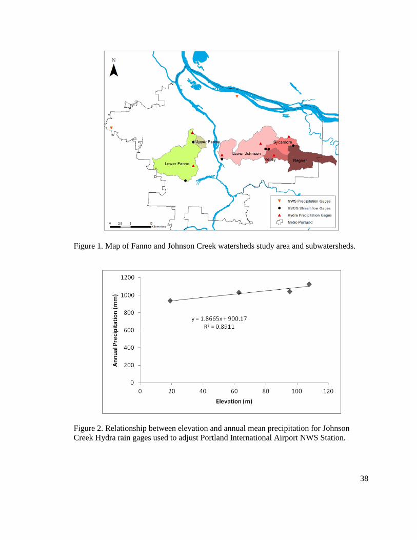
Due to the increased distance of NWS stations from Hydra stations some

differences in historical precipitation data were observed. A correlation between

increasing elevation and precipitation was determined between Hydra stations used for

Johnson Creek subwatersheds, and based upon this relationship, PDX records were

adjusted accordingly (Figure 2). To ensure better accuracy and to reduce any possible

effect of elevation changes, selection of Hydra stations was based on the closest

proximity to the USGS monitoring stations used in this study. In the case of missing

precipitation records, the missing values were corrected with the missing values from the

nearest complete Hydra station data. Missing data were directly supplemented and no

interpolation method was used as very few values were missing from historical records.

3.2 GIS analysis

A 10-meter Digital Elevation Model (DEM) was used in ArcGIS to create the

watersheds using each aforementioned USGS station location. The coordinates of these

13

stations were input into ArcGIS and used as “pour points” to delineate the watershed

boundaries. The nested watersheds produced by this method are useful for evaluating the

effect of watershed size upon different hydrologic metrics and their correlation with

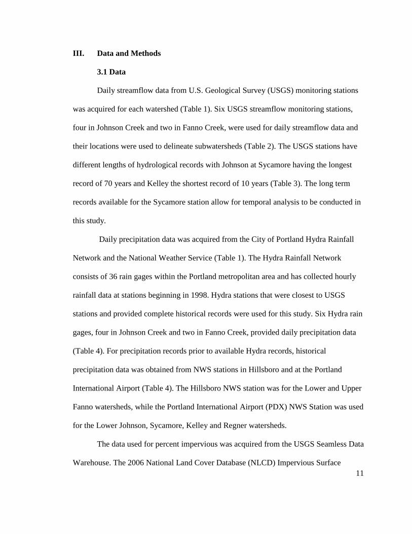
different levels of urban development. A GIS watershed dataset that accounted for

stormwater drainage was acquired through work in the Portland State Geography

Department. Using stormwater drainage networks from Clean Water Services and the

City of Portland Bureau of Environmental Services, in conjunction with a 1-m DEM, a

“piped drainage watershed” was created for the Portland Metro region. USGS station

locations were then used to delineate the six watersheds used in this study (Figure 3).

Two metrics for quantifying urbanization are utilized in this investigation; percent

impervious, and road density. Creation of both urbanization metrics required data

manipulation in ArcGIS. The impervious surface data obtained from the NLCD required

re-projection, clipping to study watersheds, and averaging of raster cells to obtain percent

impervious values for each watershed. Road density (km/km2) was calculated using GIS

streets data from Metro’s Regional Land System Information (RLIS 2012). The streets

file was clipped to the study watersheds and overall length of the roads within each

watershed was then calculated. The overall length of streets was then divided by the

watershed area to give the road density.

3.3 Hydrologic metrics

Three hydrologic metrics were utilized in this investigation: the mean annual

runoff ratio (Qa), the mean seasonal runoff ratio (Qw or Qd), and the fraction of time that

streamflow exceeds the daily mean throughout the year (TQmean). The mean annual

runoff ratio (Qa) is the ratio of runoff depth to precipitation. Runoff depth is the depth to

14

which the drainage area would be covered in water if all the water for the year was

distributed evenly over its surface (Chang 2007). Runoff depth is calculated by dividing

the yearly discharge by the watershed area. Qa is closely associated with the amount of

impervious cover and is thought to be lowest in the least urbanized watershed. The mean

seasonal runoff ratio is the ratio of seasonal runoff depth (wet season Qw or dry season

Qd) to seasonal precipitation. In this case the wet season is defined by the period of

October to March and the dry season is April to September. This seasonal division is

typical for hydrological investigations in the Pacific Northwest (Cannon and Whitfield

2001) and has been used to investigate seasonal differences within watersheds (Chang

2007). TQmean is the fraction of time that streamflow exceeds the daily mean streamflow

during the year. TQmean is an indicator of flashiness and tends to vary inversely with the

amount of urban development (Konrad 2005). TQmean values were calculated for each

watershed for the period of record and compared with the urbanization metrics.

In addition to the three hydrologic metrics used to evaluate stream behavior, the

relative change in streamflow in response to storm events was examined. There is a direct

response between precipitation events and increases in streamflow, and an evaluating the

differences in streamflow in response to rain events provides further insight to

hydrological differences that may exist due to varying amounts of urban development.

Using criteria previously used in hydrologic studies of the Pacific Northwest (Cannon

and Whitfield 2001; Chang 2007), storms are defined as continuous rainfall with more

than 2mm of rain in an hour. The study period for this analysis was limited to two and

half water years (2009-2011) spanning five seasons (3 Dry and 2 Wet). An additional dry

season was utilized to evenly represent both seasons, as the wet season typically has more

15

storm events. Due to the large number of storms, especially during the wet season, storms

preceded by dry periods were selected for with additional criteria. Dry period criteria

consisted of no more than 2mm of rainfall per day in the two days preceding the storm

event. This was done to reduce the effect of antecedent moisture conditions on the storm

analysis and provide a clearer picture of storm response due to rainfall. Using the same

criteria as Chang (2007) changes in streamflow relative to pre-storm levels were defined

as the normalized difference between baseflow and peakflow.

The normalized changes in streamflow were plotted against the normalized storm

amount for all storm events for the Lower Fanno and Lower Johnson watersheds. There

were 43 storms that fit the selection criteria for Lower Fanno watershed (19 wet season

and 24 dry season), and 47 storms for the Lower Johnson watershed (21 wet season and

26 dry).

3.4 Statistical analysis

Descriptive and inferential statistics are used to evaluate any differences between

watersheds and any links between hydrologic metrics and urbanization metrics. Box-

whisker plots are used to visually inspect for any differences that may exist for each

metric between watersheds. The Kruskall-Wallis test is the one-way analysis of variance

(ANOVA) for non-parametric data, and was used here to detect any statistical differences

that may exist among hydrologic characteristics in each watershed. The Mann-Whitney

test, a non-parametric test for testing two observations or paired data, was used to

compare the mean seasonal runoff ratios (Qw and Qd) for each watershed. Kendall’s rank

correlation test was used to compare the three hydrologic metrics values to road density

and percent impervious for all of the study watersheds. The long-term streamflow records

16

in the Sycamore watershed allowed for comparing trends for the 1941-2010 water years.

The 2011 water year was not used to provide an even 70 year record, which was then

split in two different ways; 10 year divisions were used to evaluate any decadal temporal

trends and 35 year divisions (1941-1976 and 1977-2011) were used to evaluate any

temporal trends, providing pre- and post-development periods.

17

IV. Results

4.1 Urbanization Metrics

The level of urbanization in each watershed was expressed in terms of percent

impervious and road density (km/km2). The two metrics were found to be highly

correlated with a Pearson correlation value of 0.91 (Table 5). While the metrics were

highly correlated, they quantify urbanization differently as the most urbanized watershed

is different for each metric. Road density is greatest in the Upper Fanno watershed, while

percent impervious is greatest within Lower Fanno watershed (Table 5). Both road

density and percent impervious were the lowest within the Regner watershed. Both

metrics were compared with the three hydrologic metrics for each watershed and the

relationships are discussed below.

4.2 Mean Annual Runoff Ratio (Qa)

The Kruskall-Wallis test revealed statistical difference among watersheds for Qa

values (Table 6). Box-whisker plot analysis describes the overall distribution of Qa values

and identified outliers (Figure 4). The Regner watershed was found to have the highest Qa

of 0.67, while the Upper Fanno watershed had the lowest at 0.49 (Table 7). Scatterplot

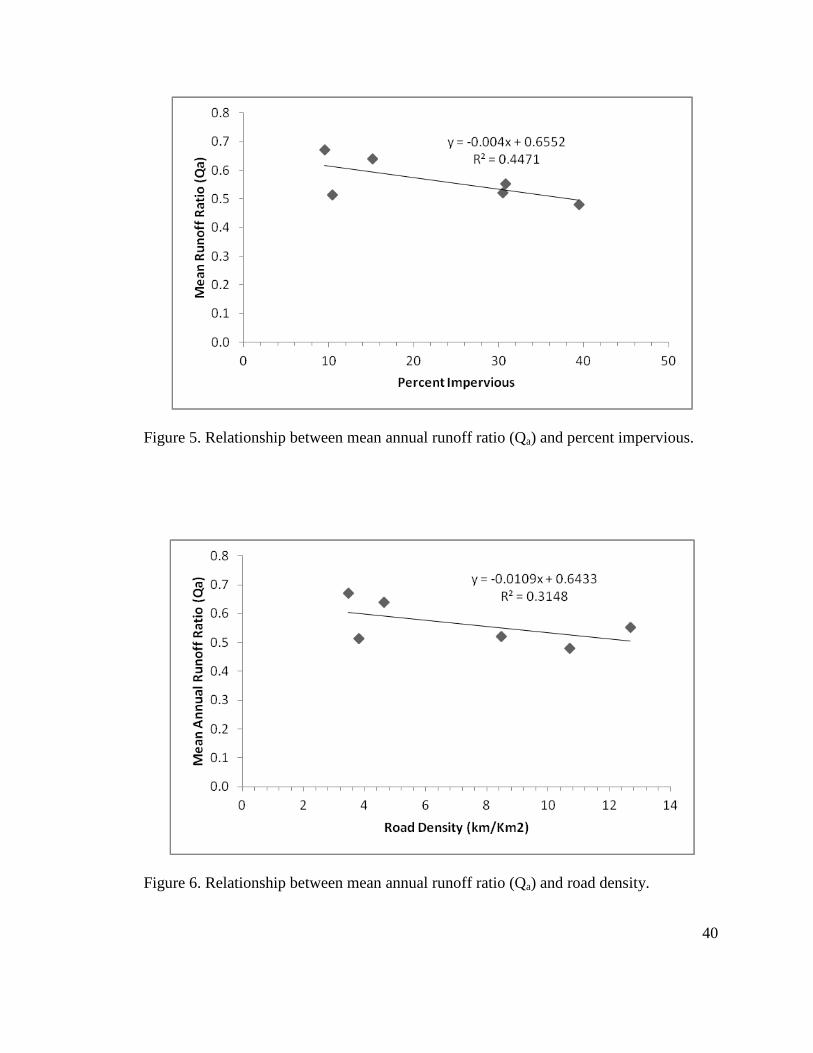
analysis shows a decreasing trend in Qa and the level of urbanization (Figure 5 and 6).

One-sided Kendall’s correlation rank test did not reveal a significant correlation between

Qa and percent impervious (τ = -0.333, p = 0.174). A negative correlation (τ = -0.467)

with road density was only significant at p < 0.10 (Table 8). The Sycamore watershed

displayed no significant trend when comparing 1941-1976 and 1977-2011 periods (Table

9). When 10 year periods were evaluated the 1941-1950 period exhibited a significant

18

increasing trend in Qa (τ = 0.442, p = 0.045). The 2001-2010 period observed a weaker

increasing trend in Qa (τ = 0.333, p = 0.090).

4.3 Mean Seasonal Runoff Ratio (Qw or Qd)

Mann-Whitney tests revealed statistically significant seasonal differences in all

watersheds except for the Lower Johnson and Lower Fanno watersheds (Table 10). The

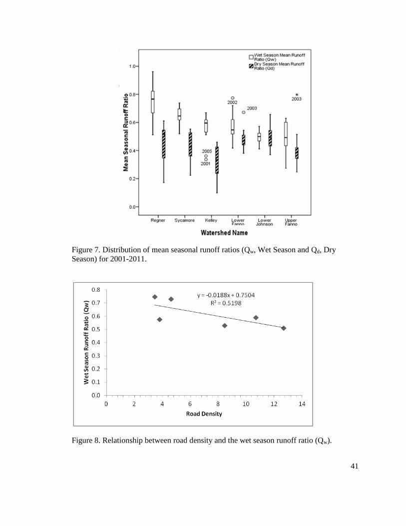
greatest differences between the wet season runoff ratio and dry season runoff ratio were

found within the Sycamore, Kelley, and Regner watersheds (Table 11). The Regner

watershed had the highest wet season runoff ratio with 0.75, while the Upper Fanno

watershed had the lowest with 0.52 (Figure 7). The Lower Johnson watershed had the

highest dry season runoff ratio with 0.51, while the Kelley watershed had the lowest with

0.33.

Trend analysis of the seasonal runoff ratios in the Sycamore watershed revealed a

significant positive trend in Qd values during the 1941-2010 period (Table 9). When the

study period is divided by decade, there was a significant increasing trend for 1951-1960

followed by a decreasing trend in the 1961-1970 period. There was no significant trend

for Qw during the 1941-2010 period however, a significant increase was observed for

1941-1950 while a weak increase was found for 2000-2010 (p < 0.10).

Road density was negatively and significantly correlated (τ = -0.600, p = 0.045)

with the wet seasonal runoff ratio (Qw) for the study watersheds. Scatterplot analysis

displays the decreasing trend of Qw as road density increases (Figure 8). Percent

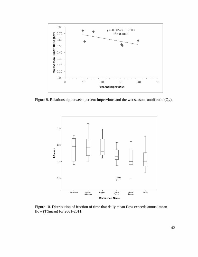
impervious also revealed a negative correlation with Qw with τ = -0.467, however it was

only significant at α = 0.094. Scatterplot analysis also displays a decreasing trend in Qw

as percent impervious decreases (Figure 9). Road density and percent impervious were

19

both positively correlated with the dry season runoff ratio (Qd). However, neither was

statistically significant with τ = 0.200 and 0.333 and p = 0.287 and 0.174, respectively.

4.4 TQmean

Flashiness, which describes the tendency of urban streams to exhibit quick rise

and fall of peak streamflow, is represented here with TQmean. TQmean values of urban

streams are generally less than 0.3, while more rural streams have values greater than 0.3

(Konrad et al. 2007). The lowest TQmean values were in the Upper Fanno and Kelley

watersheds, both with a TQmean of 0.24 (Figure 10). The highest TQmean value 0.34 was

in the Regner watershed, the most rural of the watersheds in this study with the lowest

percent impervious and road density values (Table 5). The Kruskall-Wallis test revealed

statistical difference among watersheds for TQmean values, demonstrating the differences

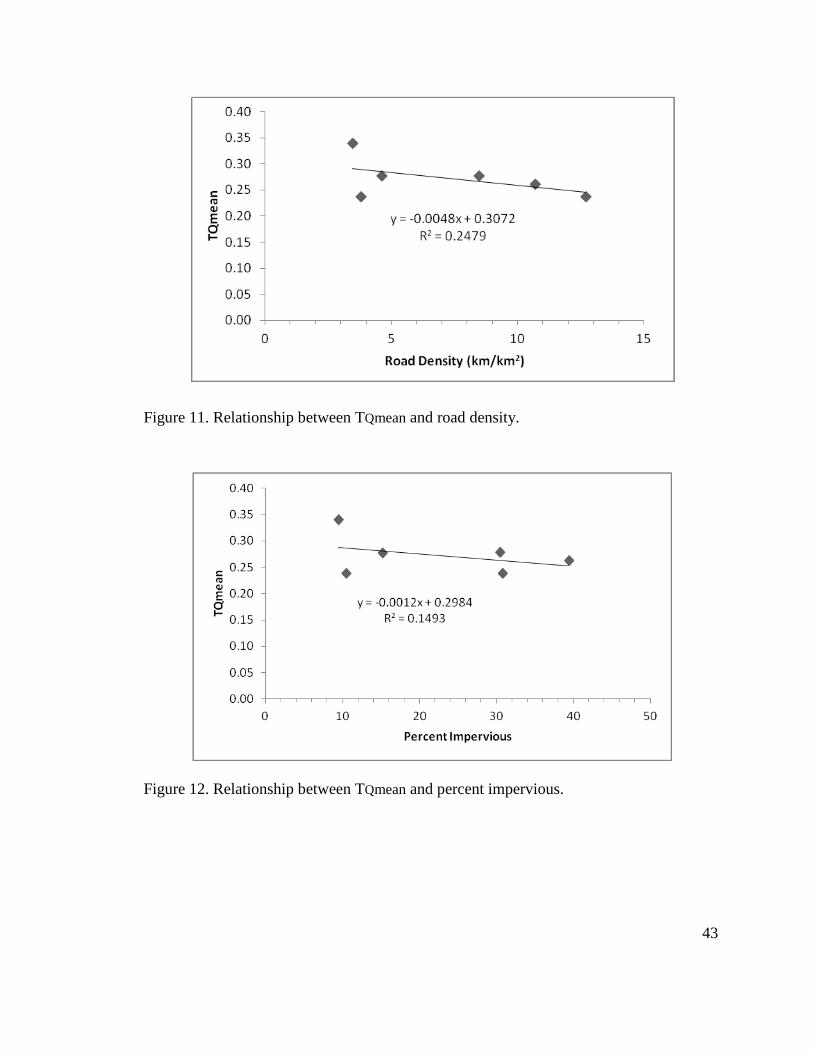
in values were not due to chance (Table 6). Negative correlations were found between

TQmean and both road density and percent impervious, τ = -0.414 and τ = -0.276

respectively, but neither were statistically significant with p = 0.126 and 0.222.

Scatterplot analysis displayed a decreasing trend in TQmean as both road density and

percent impervious increase (Figure 11 and 12). Temporally, there was no significant

trend in TQmean values during the 1941-2010 period (Table 9). When the study period is

divided by decade some temporal trends became apparent. There was a negative and

significant correlation for the 1971-1980 period (τ = -0.467, p = 0.030). The preceding

1961-1970 period observed a weaker correlation, however it was not significant at p <

0.05 (τ = -0.333, p = 0.090).

20

4.5 Storm Response Analysis

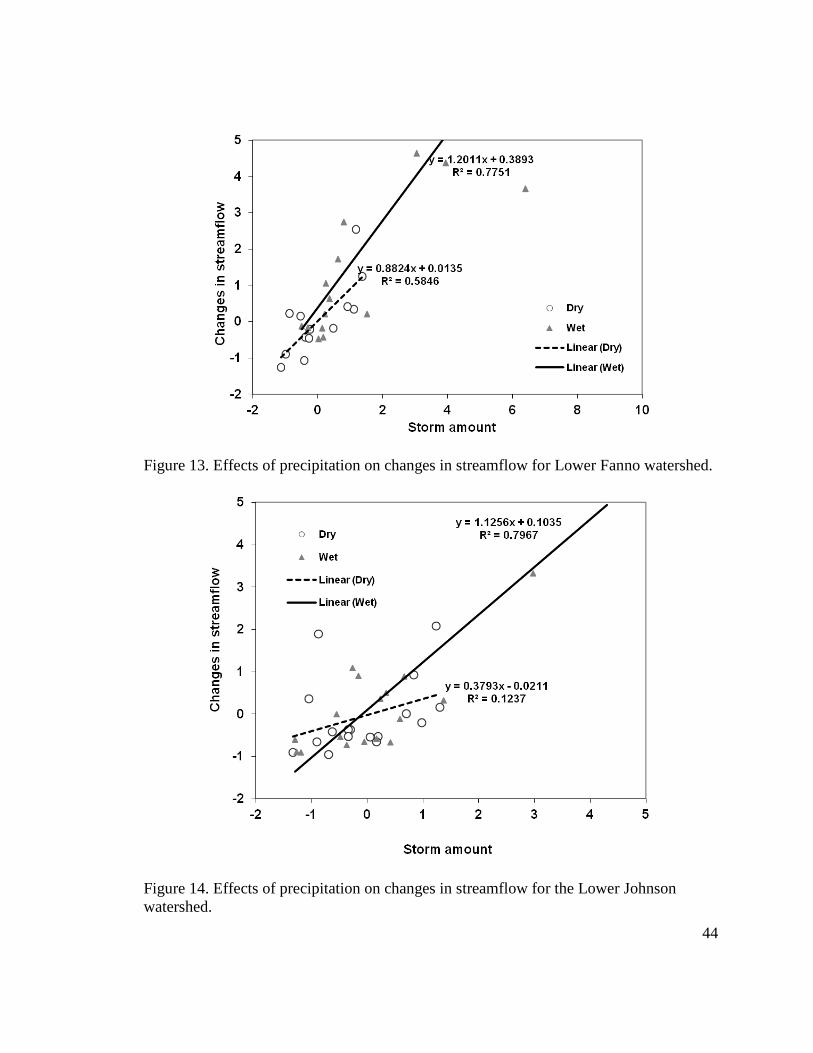
The Lower Fanno watershed experiences quick response to precipitation events

regardless of the season (Figure 13). When the normalized changes in streamflow are

plotted with the normalized storm amount, both the wet season and dry season exhibit

steep slopes, indicating a quick response to rainfall (1.22 and 0.88 respectively). The

Lower Johnson exhibited a quick response to storms in the wet season with a response

slope of 0.79 when plotted. However, unlike the Lower Fanno, the Lower Johnson

displayed had a much slower response to summer storms with a response slope of 0.12

(Figure 14).

21

V. Discussion

5. 1 Discussion: Qa

Mean annual runoff ratio is thought to be closely linked with the amount of

urbanization within a watershed, with higher Qa values in urbanized watersheds and

lower Qa values in more rural watersheds. Interestingly, the highest runoff ratio was

found within the Regner, the least urbanized watershed in the study. While low runoff

ratios are generally observed within rural areas, the higher Qa could be attributed to

factors not considered by the hydrologic metric. The Regner watershed’s higher elevation

means that it receives orographic precipitation, as well as lower evapotranspiration rates

contributing to increased runoff. Consolidated sands and gravels make up the underlying

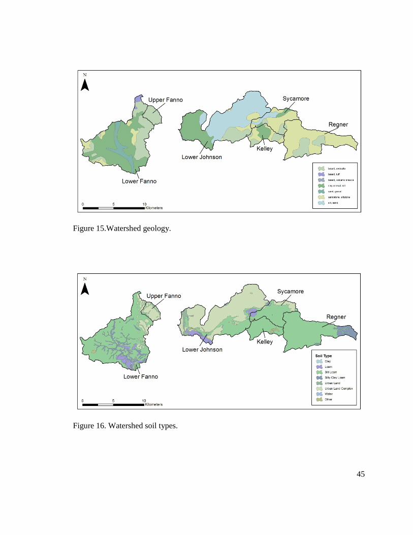
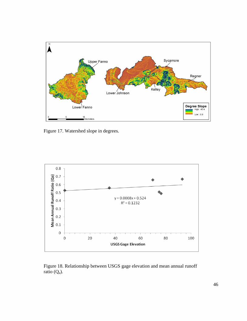
geology (Figure 15) and soils are consist primarily silty clay and silt loam (Figure 16).

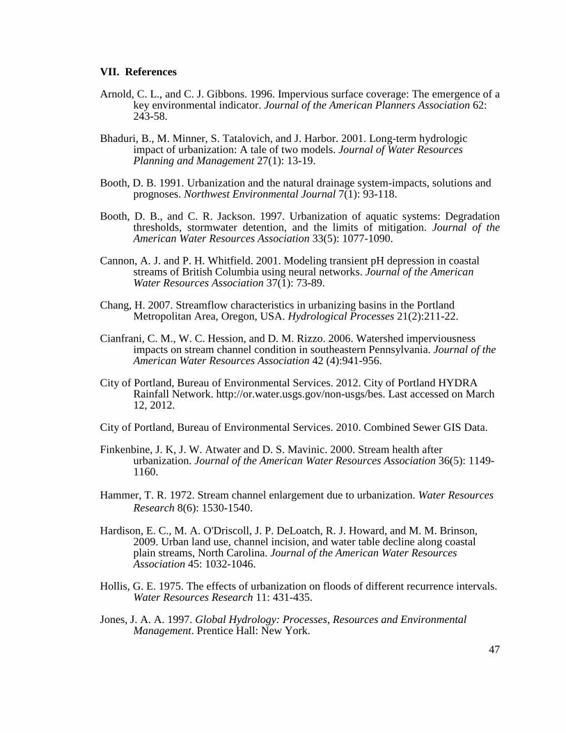
The less permeable soils and somewhat steep slopes (Figure 17) coupled with higher

precipitation contribute to greater surface runoff and streamflow (Lee and Snyder 2009).

The lowest Qa was observed in the well developed Upper Fanno watershed. Some

stormwater drainage pipes do not always drain into the same watershed where they

collect precipitation, instead routing runoff into a nearby drainage area. This could result

in overestimated precipitation while calculating the runoff ratio and produce in

unexpected low runoff ratio values. While the Upper Fanno consists of dense suburban

development and a network of stormwater drainage pipes collecting surface water the

differences in topographic watershed and piped drainage watershed areas for the Upper

Fanno are negligible (6.09 km2 and 6.03 km2 respectively), so this factor does not appear

to be influencing the low Qa value. The underlying geology consists of volcanic basalt

(Figure 15) while the soils consist primarily of silty loams and urban complex (Figure

22

16). The less permeable soils, high levels of impervious surfaces and steep slopes (Figure

17) would normally suggest higher Qa values, however this is not case with the Upper

Fanno. It is unclear from this investigation what is contributing to the low runoff ratios in

the Upper Fanno watershed and further investigation is necessary to explain these values.

Percent impervious was not significantly correlated with Qa, however road density

was negatively correlated (τ = -0.467) but only significant at p < 0.10. The weak

relationship suggests that urbanization can result in changes in the annual runoff ratio, but

that other factors besides urbanization may influence Qa. Similar research has also

suggested that urbanization may not be the most important factor for predicting total

annual runoff (Rose and Peters 2001; Chang 2007). Total annual flow may not change

significantly, but the composition of surface water and groundwater contributions may

change. In response to urbanization, surface runoff contributions may increase, while

groundwater contributions decrease. Previous research has also suggested that annual

scales may not capture the dynamic behavior of urban streamflow (Chang 2007). Shorter

time scales, possibly monthly or event scale, may be better suited for analysis. Increased

surface runoff may be offset by lower groundwater contributions due to impervious

surfaces and Qa may fail to capture this behavior.

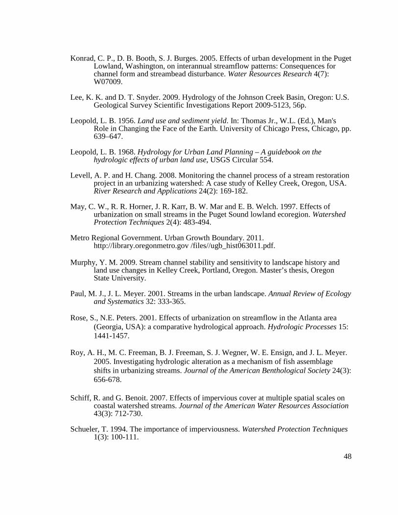
Overall, a general decrease in runoff ratios was observed from higher elevation

watersheds to lower elevation watersheds (Figure 18). Similarly, this pattern of

decreasing runoff ratios with decreasing elevation was observed in Rose and Peter’s

(2001) comparison of streamflow characteristics in the Atlanta, Georgia area. They

contributed this pattern to higher rates of evapotranspiration (ET) at lower elevation

watersheds which returns more precipitation back to the atmosphere. Chang (2007)

23

observed a similar pattern in their evaluation of Johnson Creek, attributing higher ET

values to the watershed’s elongated shape and warmer stream temperatures.

The Sycamore watershed’s long period of record allowed temporal trends in Qa to

be evaluated. The moderately developed Sycamore watershed had the second highest Qa

of the watersheds at 0.66, so to investigate any temporal trends Qa existed due to

urbanization, Kendall’s rank correlation was evaluated. While no significant change was

observed when considering the entire period of record, the earliest and most recent

portions indicated the influence of urbanization. The early increase in the mean runoff

ratio for 1941-1950 could be due to the initial pressure of urbanization, while the middle

part of the record indicates that Qa may have stabilized after the initial urbanization of the

area (Table 6). The recent increase in Qa during the 2000-2010 period could indicate

more recent pressure of urbanization in the watershed due to the expansion of the UGB

that occurred in 2002. The expansion of the UGB means that the Sycamore watershed

will experience higher rates of urbanization and this could produce changes in Qa as the

hydrologic properties of the watershed are altered. It should be noted that Kelley and

Regner watersheds, which are nested in the Sycamore watershed, did not see any

significant changes in Qa (τ = -0.256, p = 0.111 and τ = 0.200, p = 0.196 respectively).

However, both Kelley and Regner watersheds were limited to short periods of records

with 10 and 13 years of data respectively.

5.2 Discussion: Qw and Qd

Seasonal differences in streamflow can vary greatly within the Pacific Northwest

due to the climate, which consists of mild and wet winters and dry, warm summers.

Winter precipitation accounts for about 80% of total annual precipitation for the Portland

24

metro area (Chang 2007). The mean seasonal runoff ratios (Qw and Qd) were used to

investigate any seasonal differences that may exist in watersheds. It was expected that

seasonal differences in the runoff ratio would be greatest within the most urbanized

watersheds. Wet season runoff ratios were found to be highest in the Sycamore and

Regner watersheds (Figure 7). Sycamore is a moderately urbanized watershed with a road

density of 4.6 (km/km2) and 15.2% impervious. An elevated wet season runoff ratio can

be attributed to the flash runoff from impervious surfaces during the wet season.

It was hypothesized that seasonal differences between runoff ratios would be

greatest within the most urbanized watersheds. Mann-Whitney tests revealed statistically

significant seasonal differences in all watersheds except for the Lower Johnson and

Lower Fanno (Table 11) watersheds and the box-whisker plots display the small seasonal

differences (Figure 7).

The moderately developed Sycamore watershed exhibited the second largest

difference between runoff ratios with 0.65 and 0.39 for winter and summer respectively.

While Sycamore is moderately developed with 15.2% impervious and 4.6 road density,

the more urbanized watersheds of Upper Fanno, Lower Fanno and Lower Johnson did not

display large seasonal difference as expected. Lower Johnson had the highest dry season

runoff ratio of 0.51 and the smallest seasonal difference in runoff ratios (Qw = 0.53 and

Qd = 0.51). The high dry season runoff ratio and consequently the small difference in

seasonal runoff ratios could be attributed to the presence of Crystal Springs Creek which

enters Johnson Creek just north of the Johnson Creek at Milwaukie USGS gage. Lee and

Snyder (2009) noted that Crystal Springs provides most of the late summer season flow

for the Lower Johnson Creek. Crystal Springs Creek also accounts for about half of the

25

increase in streamflow observed from the Sycamore to Milwaukie stations. The

contributions of Crystal Springs Creek to Lower Johnson streamflow therefore reduces

the seasonal differences that would be expected in such a highly developed watershed.

Additionally, underground injection control (UIC) systems such as dry wells, stormwater

injection systems and sumps, all divert stormwater into the subsurface (Lee and Snyder

2009). Smaller stormwater contribution to streamflow particularly impacts the wet season

runoff ratio as a proportion of storm runoff is diverted, and this is not reflected in Qw.

Interestingly, the least urbanized watershed Regner, had the highest wet season

runoff ratio and exhibited the greatest difference in seasonal runoff ratios where Qw =

0.75 and Qd = 0.46. Regner may have lower ET losses due to the higher elevation of the

watershed compared to lower elevation watersheds, and therefore more precipitation

contributes to wet season flow.

Scatterplot analysis indicated a decreasing trend in Qw as the level of urban

development increases (Figure 8 and Figure 9). It was expected that wet season runoff

ratios would be higher in watersheds with more urbanization due to increase surface

runoff. However, as with Qa, increased surface runoff may be offset by lower

groundwater contributions due to impervious surfaces. While road density and percent

impervious were both positively correlated with the dry season runoff ratio (Qd) in the

study watersheds, neither was statistically significant (Table 8). A significant correlation

between Qd and watershed size (τ = 0.600, p = 0.045) indicates that larger watershed size

results in higher Qd values (Table 12).

It was expected that watersheds with greater levels of development would exhibit

significant differences between Qw and Qd due to urbanization. Increased surface runoff

26

due to impervious surfaces, in addition to extensive stormwater drainage systems that

route runoff into nearby streams at a faster rate, typically produces higher wet season

runoff. As with Qa, it is possible that seasonal differences in highly urbanized watersheds

may not be captured at this temporal scale (seasonal as opposed to annual with Qa), and

may instead require the use of daily or hourly metrics to measure changes. Elevation may

play a role as ET losses may account for Regner watersheds large difference between Qw

and Qd.

5.3 Discussion: TQmean

TQmean is a measure of a watershed’s flashiness and is inversely related to urban

development. It was hypothesized that the watersheds with the highest levels of urban

development would exhibit the lowest TQmean values. Watersheds with higher levels of

urban development tend to have fewer days where daily mean flow exceeds the annual

mean flow (Figure 10). The lowest TQmean values were in the Upper Fanno and Kelley

watersheds, both with a TQmean of 0.24. Low TQmean values in Upper Fanno and Kelley

watersheds indicate a flashy response to precipitation, with faster storm recession and

lower baseflow contributions during the wet season. The low TQmean value in the Upper

Fanno is expected since it is highly developed with a road density of 12.7 (km/km2) and

30.8% impervious. A low TQmean value in the Kelley watershed is interesting

considering the low levels of development with 10.4 % impervious surface and a road

density of 3.8 (km/km2). Kelley watershed does not appear to be losing any precipitation

inputs due to stormwater drainage being routed outside the system, as the difference in

watershed size when considering the drainage network is minimal (Table 13). It is

possible that other watershed characteristics not directly considered here, such as soils or

27

geology may also influence TQmean. Another consideration is that while Kelley has low

levels of development, it is still beyond what some experts have termed a “critical

threshold” value of 10% for urban development (Booth, 1991; Schueler 1994). This

means that watersheds see the most changes to the hydrologic regime when moving from

0% or nearly 0% up to 10%. This could make it difficult to identify clear TQmean patterns

in watersheds with beyond the 10% developed threshold. While a clear relationship

between low TQmean and urbanization was not established, the least developed Regner

watershed had the highest TQmean as expected.

Temporal analysis in Sycamore revealed a significant decrease in TQmean for the

1971-1980 period (Table 9). It is hard to directly link this decrease with urban

development as much of the infrastructure already existed prior to the beginning of this

period (Lee and Snyder, 2009). The preceding 1961-1970 period observed a weaker rank

correlation, however it was not significant at p < 0.05 (τ = -0.333, p = 0.090). This short

decreasing trend in TQmean indicates an increase in flashiness. However it is unclear

what caused this trend and it is not believed to be linked with any urban development.

On the rural to urban gradient a declining trend in TQmean values can be observed

(Figure 11 and 12). While statistical analysis revealed a negative correlation between

TQmean and both road density and percent impervious neither were statistically

significant (p = 0.126 and 0.222 respectively). The rural Kelley watershed (3.8 road

density and 10.4% impervious) exhibited a TQmean value 0.24 over the study period,

lower than was expected and comparable to more urban streams in the study. Upper

Fanno exhibited the same TQmean value of 0.24 but is significantly more urbanized with

a 12.7 road density (km/km2) and 30.8% impervious. As was the case with Qa, a lower

28

than expected TQmean value may be the result of water leaving the system through the

stormwater drainage system. High levels of urbanization have been shown to result in

flashy urban streams (Roy et al. 2005). A weak rank correlation (τ = 0.414, p = 0.126)

between TQmean and watershed size indicates that the drainage area does not likely have

much of an effect upon the relationship between TQmean and both road density and

percent impervious.

Due to the flashy nature of Johnson Creek and its history of flooding, it was

hypothesized that a decreasing trend in TQmean would be exhibited by examining the

Sycamore station long term record. This decreasing trend could be associated with

increasing development and possibly the creation of the Oregon land use laws in 1973

and creation of the UGB in 1978. The periods after 1980 show no significant decrease

and could be associated with the relatively stable development of the watershed.

5.4 Discussion: Storm Response Analysis

Wet season storms produced steep changes in streamflow for both the Lower

Fanno and Lower Johnson Watershed. This suggests the influence of antecedent soil

moisture on stream response as well as increased surface runoff due to impervious

surfaces. Summer storms produced a much steeper response in the Lower Fanno than the

Lower Johnson. The steep response in summer storms for the Lower Fanno is attributed

to rapid surface runoff. While the Lower Johnson is highly urbanized, the combined

sewer system collects surface water from much of this area and well drained soils create a

slower response for summer storms.

29

VI. Conclusions

It was determined that urbanization in Fanno and Johnson Creek, and their

subwatersheds, has resulted in changes to streamflow characteristics. While it was

hypothesized that the annual mean runoff ratio would be lower in watersheds with high

levels of urbanization, no significant trends were found. There were some temporal

changes in Qa in the Sycamore watershed, indicating that urbanization can have an effect

upon the annual runoff ratio, however it may not be the best hydrologic metric to

demonstrate the hydrologic effects of urbanization. This indicates the effects of

urbanization may not be adequately captured on an annual scale and that the mean annual

runoff ratio simply fails to capture most of these changes. Further illustrating this was the

lack of a significant relationship between measures of urbanization and Qa.

The negative correlation between urbanization and Qw indicated a decreasing

trend in Qw with urbanization. Qw was expected to be higher in more developed

watersheds but as previously mentioned, even at a shorter seasonal scale, Qw may fail to

accurately describe seasonal effects of urbanization. Additionally, differences between

seasonal runoff ratios were found to be greatest in more rural watersheds than in

urbanized watersheds. It is likely that the differences in soil permeability and the

interception of precipitation by the combined sewer, and UIC moderates the high flows in

the Lower Johnson. The Sycamore’s trend analysis revealed some significant increases in

Qw during late and early periods of record, indicating some influence of urban

development on wet season flow. However, the overall increase Qd was not expected as

urbanization should decrease baseflow contributions which account for a large proportion

of summer flow in the Pacific Northwest.

30

Generally, the more urbanized streams exhibited lower TQmean values than rural

streams in this study. Neither road density nor percent impervious proved to be a reliable

predictor of TQmean values. However, while trend analysis in the Sycamore watershed

did indicate some significant increases in flashiness it is not believed to be associated

with historical development in the watershed.

There are two main conclusions of this study. First, the time scale used seems to

have a large impact upon the ability to characterize the influence of urbanization on

streamflow characteristics. Using Sycamore’s long term records, it was possible to isolate

some trends in each metric, however, the general pattern was not always evident. This

has been attributed to the time scale for analysis being too large to capture the dynamic

behavior of urban streams. Using an event scale analysis may be better suited to capture

the quick response of urban streams to precipitation events. The limited event scale

analysis performed in this study revealed interesting insights to the different behavior of

the Lower Johnson and Lower Fanno watersheds.

Second, the Johnson Creek watershed, in particular the Lower Johnson, does not

behave as a “typical” urban watershed. This is partly attributed to the historical

development and associated drainage infrastructure, which includes a combined sewer

system and UICs. Stormwater drainage networks that route water directly into the stream

or out of the watershed completely complicate the process of characterizing streamflow.

Also contributing to the unique streamflow behavior of Johnson Creek is the

hydrogeologic properties that vary over the watershed. The northern side of the

watershed is generally flat except for isolated volcanic buttes, and has well drained soils

while the southern side is comprised of steep slopes and less-permeable soils which

31

contribute more to more rapid runoff. Groundwater contributions which comprise most of

Crystal Springs also are responsible for unexpected hydrologic metric values, most

notably the lack of difference in seasonal runoff ratios Qw and Qd.

Future recommendations for study include applying a smaller temporal scale for

hydrologic analysis to better characterize effects of urbanization on streamflow patterns.

Utilizing hydrologic metrics that operate on shorter time scales and a comparison of those

with urbanization metrics is recommended. The limited use of storm scale analysis in this

study was effective at illustrating the different response to rainfall in Fanno and Johnson

watersheds. Incorporating the influence of the metropolitan areas stormwater drainage

system in further detail would be beneficial as this system can significantly alter natural

drainage characteristics. While the difference in topological watershed and piped

drainage watershed areas was considered as a cofounding factor in this study’s results,

further analysis is recommended.

32

Table 1. Data types and sources used for the study.

Category Data Source

Hydrology Historical streamflow USGS Oregon Water Science Center

Climate Historical precipitation Hydra Rainfall Network NOAA National Climate Data Center

Soil Hydrologic Soil Groups National Resource Conservation Service

Percent Impervious 2006 Impervious Surfaces Dataset National Land Cover Database (NLCD) 2006

Impervious Surfaces Dataset

Watersheds 10m Digital Elevation Model (DEM) US Geological Survey (USGS)

Imagery 1m Compressed County Mosaic Aerial Image, 2009

National Agricultural Imagery Program (NAIP)

Ancillary Streams, Roads, etc. Regional Land Information System (RLIS)

33

Table 2. USGS monitoring stations and hydrologic characteristics.

Station Name

Watershed Name

USGS Station

No. Location

Gage Elevation

(m)

Watershed Area (km2)

Watershed

Slope (degrees)

Watershed Elevation Range

(m)

Mean Annual Flow (m3s-1)

Johnson Creek at Milwaukie

Lower Johnson 14211550 Lat 45°27'11",

Long 122°38'31" 0.0 137.8 4.6 7.0 - 342.9 2.2

Johnson Creek at Sycamore Rd.

Sycamore 14211500 Lat 45°28'40", Long 122°30'24" 69.6 69.4 6.4 70.1 - 342.9 1.5

Kelley Creek at 159th Ave. Kelley 14211499 Lat 45°28'37",

Long 122°29'50" 74.7 12.7 6.8 73.2 - 342.9 0.2

Johnson Creek at Regner Rd.

Regner 14211400 Lat 45°29'12", Long 122°25'14" 93.0 39.8 6.2 93.0 - 331.0 0.9

Fanno Creek at Durham Ave.

Lower Fanno 14206950

Lat 45°24'13", Long

122°45'13" 35.3 80.6 5.1 36.0 - 326.1 1.2

Fanno Creek at 56th Ave.

Upper Fanno 14206900

Lat 45°29'17", Long

122°44'01" 76.2 6.1 9.0 77.1 - 324.9 0.09

34

Table 3. Length of hydrological record for USGS stations.

Station Name USGS Station No. Date Range (Water Years) Water Years

Johnson Creek at Milwaukie 14211550 1990-2011 22

Johnson Creek at Sycamore Rd. 14211500 1941-2011 71

Kelley Creek at 159th Ave. 14211499 2001-2011 11

Johnson Creek at Regner Rd. 14211400 1999-2011 13

Fanno Creek at Durham Ave. 14206950 1994-1995, 2001-2011 13

Fanno Creek at 56th Ave. 14206900 1991-2011 21

Table 4. Weather stations used for precipitation records.

Station Name Source Station No. Location Elevation (m)

Mean Annual Precipitation

(cm) Portland Intl.

Airport NWS 356751 Lat 45°35'27", Long 122°36'01" 6 98

Harney Hydra 64 Lat 45°27'44", Long 122°38'36" 19 93

Holgate Hydra 21 Lat 45°29'21", Long 122°31'26" 63 103

Pleasant Valley Hydra 145 Lat 45°27'52", Long 122°28'50" 108 113

Gresham Fire Dept. Hydra 20 Lat 45°30'27", Long 122°26'12" 95 104

Hillsboro NWS 353908 Lat 45°30'50", Long 122°59'24" 49 98

Sylvania PCC Hydra 4 Lat 45°26'13", Long 122°43'54" 197 90

Sylvan School Hydra 161 Lat 45°30'36", Long 122°44'13" 247 85

Table 5. Urban development in each watershed represented by road density and percent impervious and correlation.

Watershed Road Density (km/km2) Percent Impervious Lower Johnson 8.5 30.5 Sycamore 4.6 15.2 Kelley 3.8 10.4 Regner 3.5 9.5 Lower Fanno 10.7 39.5 Upper Fanno 12.7 30.8 Pearson Correlation Coefficient r = 0.912 , p = 0.01

35

Table 6. Kruskall-Wallis test for testing independence of hydrologic metrics among watersheds. Bold values are statistically significant at p < 0.05.

Hydrologic Metric Chi-Squared p-value

Qa 23.28 0.00

Qw 28.48 0.00

Qd 14.30 0.01

TQmean 12.52 0.03

Table7. Mean annual runoff ratios (Qa) for each watershed.

Watershed Qa

Lower Johnson 0.53

Sycamore 0.66

Kelley 0.51

Regner 0.67

Upper Fanno 0.49

Lower Fanno 0.56 Table 8. Kendall’s tau rank correlation values between hydrologic metrics and urbanization metrics. Bold values are statistically significant at p < 0.05.

Road Density Percent Impervious

tau p tau p

Qa -0.467 0.094 -0.333 0.174

Qw -0.600 0.045 -0.467 0.094

Qd 0.200 0.287 0.333 0.174

TQmean -0.414 0.126 -0.276 0.222

36

Table 9. Trend analysis for each hydrologic metric for the Sycamore watershed. Bold values are significant at p < 0.05.

Qa Qw Qd TQmean

tau p tau p tau p tau p

1941-2010 -0.074 0.186 -0.073 0.186 0.154 0.030 0.160 0.422

1941-1950 0.442 0.045 0.511 0.020 0.067 0.394 0.067 0.394 1951-1960 -0.111 0.327 -0.156 0.266 0.422 0.045 -0.022 0.464 1961-1970 -0.111 0.327 -0.022 0.464 -0.422 0.045 -0.333 0.090 1971-1980 -0.022 0.464 -0.156 0.266 -0.022 0.464 -0.467 0.030 1981-1990 -0.255 0.185 -0.156 0.266 -0.022 0.464 -0.045 0.429 1991-2000 0.022 0.464 -0.022 0.464 -0.156 0.266 0.067 0.394 2001-2010 0.333 0.090 0.378 0.064 0.378 0.064 -0.270 0.281

Table 10. Mann-Whitney test values comparing Qw and Qd to evaluate seasonal differences. Bold values are statistically significant at p < 0.05.

Table 11. Differences in seasonal runoff ratio in comparison to levels of urbanization.

Watershed Qw Qd Seasonal Difference Road Density (km/km2)

Percent Impervious

Lower Johnson 0.53 0.51 0.03 8.5 30.5

Sycamore 0.65 0.39 0.26 4.6 15.2 Kelley 0.57 0.33 0.24 3.8 10.4 Regner 0.75 0.46 0.29 3.5 9.5 Lower Fanno 0.59 0.49 0.10 10.7 39.5 Upper Fanno 0.52 0.42 0.10 12.7 30.8

Mann-Whitney Test Values Watershed p value

Lower Johnson 0.519 Sycamore 0.000 Kelley 0.001 Regner 0.000 Lower Fanno 0.058 Upper Fanno 0.013

37

Table 12. Kendall’s tau rank correlation values between hydrologic metrics and watershed size. Bold values are statistically significant at p < 0.05.

Watershed Area

tau p

Qa 0.200 0.287

Qw 0.067 0.425

Qd 0.600 0.045

TQmean 0.414 0.126

Table 13. Watershed areas for topographic and piped drainage watershed delineations.

Watershed Topographic Watershed Area (km2) Piped Drainage Watershed Area (km2) Lower Johnson 137.77 155.29 Sycamore 69.41 70.19 Kelley 12.13 12.36 Regner 39.81 38.45 Lower Fanno 80.62 80.56 Upper Fanno 6.09 6.03

38

Figure 1. Map of Fanno and Johnson Creek watersheds study area and subwatersheds.

Figure 2. Relationship between elevation and annual mean precipitation for Johnson Creek Hydra rain gages used to adjust Portland International Airport NWS Station.

39

Figure 3. Map of Fanno and Johnson Creek “piped drainage watershed” delineated using both the topology and stormwater sewer network.

Figure 4. Distribution of mean annual runoff ratios (Qa) for 2001-2011.

40

Figure 5. Relationship between mean annual runoff ratio (Qa) and percent impervious.

Figure 6. Relationship between mean annual runoff ratio (Qa) and road density.

41

Figure 7. Distribution of mean seasonal runoff ratios (Qw, Wet Season and Qd, Dry Season) for 2001-2011.

Figure 8. Relationship between road density and the wet season runoff ratio (Qw).

42

Figure 9. Relationship between percent impervious and the wet season runoff ratio (Qw).

Figure 10. Distribution of fraction of time that daily mean flow exceeds annual mean flow (TQmean) for 2001-2011.

43

Figure 11. Relationship between TQmean and road density.

Figure 12. Relationship between TQmean and percent impervious.

44

Figure 13. Effects of precipitation on changes in streamflow for Lower Fanno watershed.

Figure 14. Effects of precipitation on changes in streamflow for the Lower Johnson watershed.

45

Figure 15.Watershed geology.

Figure 16. Watershed soil types.

46

Figure 17. Watershed slope in degrees.

Figure 18. Relationship between USGS gage elevation and mean annual runoff ratio (Qa).

47

VII. References Arnold, C. L., and C. J. Gibbons. 1996. Impervious surface coverage: The emergence of a

key environmental indicator. Journal of the American Planners Association 62: 243-58.

Bhaduri, B., M. Minner, S. Tatalovich, and J. Harbor. 2001. Long-term hydrologic

impact of urbanization: A tale of two models. Journal of Water Resources Planning and Management 27(1): 13-19.

Booth, D. B. 1991. Urbanization and the natural drainage system-impacts, solutions and

prognoses. Northwest Environmental Journal 7(1): 93-118. Booth, D. B., and C. R. Jackson. 1997. Urbanization of aquatic systems: Degradation

thresholds, stormwater detention, and the limits of mitigation. Journal of the American Water Resources Association 33(5): 1077-1090.

Cannon, A. J. and P. H. Whitfield. 2001. Modeling transient pH depression in coastal

streams of British Columbia using neural networks. Journal of the American Water Resources Association 37(1): 73-89.

Chang, H. 2007. Streamflow characteristics in urbanizing basins in the Portland

Metropolitan Area, Oregon, USA. Hydrological Processes 21(2):211-22. Cianfrani, C. M., W. C. Hession, and D. M. Rizzo. 2006. Watershed imperviousness

impacts on stream channel condition in southeastern Pennsylvania. Journal of the American Water Resources Association 42 (4):941-956.

City of Portland, Bureau of Environmental Services. 2012. City of Portland HYDRA

Rainfall Network. http://or.water.usgs.gov/non-usgs/bes. Last accessed on March 12, 2012.

City of Portland, Bureau of Environmental Services. 2010. Combined Sewer GIS Data. Finkenbine, J. K, J. W. Atwater and D. S. Mavinic. 2000. Stream health after

urbanization. Journal of the American Water Resources Association 36(5): 1149-1160.

Hammer, T. R. 1972. Stream channel enlargement due to urbanization. Water Resources

Research 8(6): 1530-1540. Hardison, E. C., M. A. O'Driscoll, J. P. DeLoatch, R. J. Howard, and M. M. Brinson,

2009. Urban land use, channel incision, and water table decline along coastal plain streams, North Carolina. Journal of the American Water Resources Association 45: 1032-1046.

Hollis, G. E. 1975. The effects of urbanization on floods of different recurrence intervals.

Water Resources Research 11: 431-435. Jones, J. A. A. 1997. Global Hydrology: Processes, Resources and Environmental

Management. Prentice Hall: New York.

48

Konrad, C. P., D. B. Booth, S. J. Burges. 2005. Effects of urban development in the Puget

Lowland, Washington, on interannual streamflow patterns: Consequences for channel form and streambead disturbance. Water Resources Research 4(7): W07009.

Lee, K. K. and D. T. Snyder. 2009. Hydrology of the Johnson Creek Basin, Oregon: U.S.

Geological Survey Scientific Investigations Report 2009-5123, 56p. Leopold, L. B. 1956. Land use and sediment yield. In: Thomas Jr., W.L. (Ed.), Man's

Role in Changing the Face of the Earth. University of Chicago Press, Chicago, pp. 639–647.

Leopold, L. B. 1968. Hydrology for Urban Land Planning – A guidebook on the

hydrologic effects of urban land use, USGS Circular 554. Levell, A. P. and H. Chang. 2008. Monitoring the channel process of a stream restoration

project in an urbanizing watershed: A case study of Kelley Creek, Oregon, USA. River Research and Applications 24(2): 169-182.

May, C. W., R. R. Horner, J. R. Karr, B. W. Mar and E. B. Welch. 1997. Effects of

urbanization on small streams in the Puget Sound lowland ecoregion. Watershed Protection Techniques 2(4): 483-494.

Metro Regional Government. Urban Growth Boundary. 2011.

http://library.oregonmetro.gov /files//ugb_hist063011.pdf. Murphy, Y. M. 2009. Stream channel stability and sensitivity to landscape history and

land use changes in Kelley Creek, Portland, Oregon. Master’s thesis, Oregon State University.

Paul, M. J., J. L. Meyer. 2001. Streams in the urban landscape. Annual Review of Ecology

and Systematics 32: 333-365. Rose, S., N.E. Peters. 2001. Effects of urbanization on streamflow in the Atlanta area

(Georgia, USA): a comparative hydrological approach. Hydrologic Processes 15: 1441-1457.

Roy, A. H., M. C. Freeman, B. J. Freeman, S. J. Wegner, W. E. Ensign, and J. L. Meyer.

2005. Investigating hydrologic alteration as a mechanism of fish assemblage shifts in urbanizing streams. Journal of the American Benthological Society 24(3): 656-678.

Schiff, R. and G. Benoit. 2007. Effects of impervious cover at multiple spatial scales on

coastal watershed streams. Journal of the American Water Resources Association 43(3): 712-730.

Schueler, T. 1994. The importance of imperviousness. Watershed Protection Techniques

1(3): 100-111.

49

Snyder, D. T. 2008. Estimated depth to ground water and configuration of the water table in Portland, Oregon area: U.S. Geological Survey Scientific Investigations Report 2008-5059.

United Nations Department of Social and Economic Affairs/Population Division. 2008.

World Urbanization Prospects: The 2007 Revision. Table A1. US Census Bureau: State and County Quickfacts.

http://quickfacts.census.gov/qfd/states/4 1/4159000.html. Last accessed 4/10/2012.