Embed Size (px)
Citation preview
Stream Water Quality Management: A Stochastic Mixed-integer Programming Model
Md. Kamar Ali Graduate Research Assistant
Agricultural and Resource Economics West Virginia University
P.O. Box 6108, Morgantown, WV 26506 Phone: (304) 293-4832 ext 4476
Fax: (304) 293-3752 e-mail: [email protected]
Jerald J. Fletcher Professor, Environmental and Natural Resource Economics and Chair, Agricultural and Resource Economics Program
Division of Resource Management West Virginia University
P.O. Box 6108, Morgantown, WV 26506 Phone: (304) 293-4832 ext 4452
Fax: (304) 293-3752 e-mail: [email protected]
Tim T. Phipps Professor, Agricultural and Resource Economics
West Virginia University P.O. Box. 6108, Morgantown, WV 26506
Phone: (304) 293-4832 ext 4474 Fax: (304) 293-3752
e-mail: [email protected] Subject code: Environmental Economics JEL Codes: Q25, C61 Paper presented at the Annual Meeting of the American Agricultural Economics Association (AAEA) in Long Beach, July 28-31, 2002. Copyright 2002 by Md. Kamar Ali, Jerald J. Fletcher, and Tim T. Phipps. All rights reserved. Readers may make verbatim copies of this document for non-commercial purposes by any means, provided that this copyright notice appears on all such copies.
1
ABSTRACT
Water quality management under the watershed approach of Total Maximum Daily Load (TMDL) programs requires that water quality standards be maintained throughout the year. The main purpose of this research was to develop a methodology that incorporates inter-temporal variations in stream conditions through statistical distributions of pollution loading variables. This was demonstrated through a cost minimization mixed-integer linear programming (MIP) model that maintains the spatial integrity of the watershed problem. Traditional approaches for addressing variability in stream conditions are unlikely to satisfy the assumptions on which these methodologies are founded or are inadequate in addressing the problem correctly when distributions are not normal.
The MIP model solves for the location and the maximum capacity of treatment plants to be built throughout the watershed which will provide the optimal level of treatment throughout the year.
The proposed methodology involves estimation of parameters of the distribution of pollution loading variables from simulated data and use of those parameters to re-generate a suitable number of random observations in the optimization process such that the new data preserve the same distribution parameters. The objective of the empirical model was to minimize costs for implementing pH TMDLs for a watershed by determining the level of treatment required to attain water quality standards under stochastic stream conditions. The output of the model was total minimum costs for treatment and selection of the spatial pattern of the least-cost technologies for treatment. To minimize costs, the model utilized a spatial network of streams in the watershed, which provides opportunities for cost-reduction through trading of pollution among sources and/or least-cost treatment. The results were used to estimate the costs attributable to inter-temporal variations and the costs of different settings for the ‘margin of safety’.
The methodology was tested with water quality data for the Paint Creek watershed in West Virginia. The stochastic model included nine streams in the optimal solution. An estimate of inter-temporal variations in stream conditions was calculated by comparing total costs under the stochastic model and a deterministic version of the stochastic model estimated with mean values of the loading variables. It was observed that the deterministic model underestimates total treatment cost by about 45 percent relative to the 97th percentile stochastic model.
Estimates of different margin of safety were calculated by comparing total costs for the 99.9th percentile treatment (instead of an idealistic absolute treatment) with that of the 95th to 99th percentile treatment. The differential costs represent the savings due to the knowledge of the statistical distribution of pollution and an explicit margin of safety. Results indicate that treatment costs are about 7 percent lower when the level of assurance is reduced from 99.9 to 99 percent and 21 percent lower when 95 percent assurance is selected.
The application of the methodology, however, is not limited to the estimation of TMDL implementation costs. For example, it could be utilized to estimate costs of anti-degradation policies for water quality management and other watershed management issues.
2
Introduction
Water quality management under the US Environmental Protection Agency’s
(USEPA) watershed approach (USEPA, 2002) incorporates the latest attempts to realize
the original goals of the Clean Water Act of 1972 (CWA): to clean-up and protect U.S.
waters from both point and non-point sources of pollution. While much progress has been
made over the past three decades, 40 percent of the U.S. waters currently do not meet
water quality standards, and about half of the nation’s 2,149 major watersheds continue
to suffer from serious water quality problems (USEPA, 1998).
In the initial years of the CWA, management efforts were primarily limited to at-
source control of discharges from individual point sources by requiring use of Best
Available Technologies (BAT) under the National Pollutant Discharge Elimination
System (NPDES; Section 402 of the CWA 1972). Attention to non-point source
discharge control was virtually non-existent because of the perceived relative severity of
the problems combined with personnel and budgetary limitations. The complexity in
identifying and determining clean-up responsibility was, and remains, a further
confounding factor.
The USEPA and other federal agencies have adopted a watershed approach to
better integrate non-point sources into the overall water quality management and
improvement effort. Simply put, the watershed approach is an attempt to develop a
collaborative approach to environmental management that incorporates all stakeholders
including the full range of government entities, the private sector, local organizations,
and special interest groups. This approach attempts to bring out the best balance among
efforts to control point-source pollution and non-point source runoff and to encourage
3
greater public involvement, accountability and progress toward clean water goals. The
focus moves away from technology-based point-by-point control to an overall water-
quality based approach (USEPA, 1998).
Since watershed level planning allows pollution control by the least-cost methods
and sources and thus provides opportunities for pollution trading, it has a promise of cost-
savings for implementation of the USEPA’s Total Maximum Daily Load (TMDL)
program. Both the TMDL program which seeks to bring degraded waters up to current
standards and anti-degradation policies designed to protect current water quality levels
can benefit from such an integrated approach. Based on a recent U.S. Environmental
Protection Agency study, the watershed approach is estimated to reduce TMDL
implementation costs by 25-50 percent over the point-by-point source control approach
(USEPA, 2001a).
Objectives
This paper presents a methodology that can incorporate economic decisions into
the watershed management process as part of an integrated management approach. The
approach takes as given the water quality standards and other exogenously determined
factors that managers face and develops a portfolio of treatment/management options that
accounts for stochastic inter-temporal variations in pollution loads in a watershed into a
framework that minimizes treatment costs. The model can be utilized to estimate
watershed-based TMDL implementation costs based on the inter-temporal maintenance
of water quality standards under a variety of conditions with a specified probability of the
‘margin of safety’. It can also be use to estimate costs for anti-degradation policies for
water quality management and other watershed management issues.
4
Motivation
Stream conditions in any watershed constantly change. Water flow as well as
pollution levels in streams vary with time and season. Traditional approaches to deal with
these types of variability developed a model based on a single observation or the average
of a few samples and then performed a sensitivity or scenario analysis on the factors
subject to change (Liebman and Lynn, 1966; Loucks et al., 1967; Fletcher et al., 1991;
and Phipps et al., 1991, 1992, 1996). In the context of mathematical programming
models, the sensitivity analysis amounts to parametric programming or post-optimality
analysis where the model is run again and again while changing the values for some of
the variables.
Other approaches that deal with variability with regard to water quality
management problems include chance-constrained programming (Charnes and Cooper,
1959, 1962, 1963; Sengupta, 1970) and first-order uncertainty analysis (Benjamin and
Cornell, 1970). In chance-constrained programming the constraints are expected to
satisfy the right-hand-side resource vector for a predetermined degree of confidence
(Lohani and Thanh, 1978; Zhu et al., 1994). In first-order uncertainty analysis the first
two moments of the variable factors are explicitly included in the model (Burges and
Lettenmaier, 1975; Burn and McBean, 1985).
What is missing in all these approaches, however, is the explicit consideration of
statistical distributions of the variable factors in the model. Shortle (1990) emphasized
this point by suggesting that for stochastic emissions, pollution control essentially
requires ‘improving the distribution of emissions’. Models based on a single observation
or mean values do not perform well when distributions of the relevant variables are not
5
normal. Averages or the mean values often hide valuable information. They are biased in
the direction of extreme observations if the distribution is skewed. The mean value can be
considered as a good representative of the data only if the true distribution is normal.
With few exceptions (e.g., Zhu et al., 1994), chance-constrained programming models
usually assume normality when the probabilistic constraints are translated into their
deterministic equivalents. First-order analysis does not require normality explicitly.
However, the first two moments inadequately describe the data if distributions are not
symmetric or normal. Higher order moments for many distributions are equally important
to modeling accuracy. In the case of water pollution abatement cost comparisons, Shortle
(1990) also pointed out that if the mean and variance of the damage function move in the
same direction, the covariance between marginal damage and changes in the emissions is
negative and abatement is beneficial. However, if the mean and variance move inversely,
the sign of the covariance is ambiguous and abatement may not be beneficial. The first-
order analysis implicitly assumes zero weight to the higher order moments than the first
two.
The US Environmental Protection Agency (USEPA) has adopted a watershed
approach to water quality management but continues to require states to promulgate and
enforce regulations to maintain water quality standards at all points throughout the year.
The implications for these USEPA imperatives for water quality management in a
stochastic environment and the inadequacy of traditional stochastic approaches dealing
with the non-normal distributions of pollution loading variables were the motivation for
developing the stochastic mixed-integer linear programming model presented in this
paper.
6
The General Model
Consider the following stylized description of the watershed management
problem. A watershed is defined as the area of land that catches rain and snow and drains
or seeps into a common point. Since water always flows downhill, there is a route with a
monotonically non-increasing elevation from any point in the watershed to what is called
the pour point. Within a watershed, overland flow and/or groundwater discharges
combine to form streams that further combine to form larger streams and rivers. The
beginning streams are called headwater streams or tributaries, the point where two or
more streams join is referred to as node, and the stream reach joining two nodes defines
downstream segments. The watershed area can be divided into sub-watersheds or
catchments associated with each stream segment. Pollution loading in a tributary can
come from non-point or point sources within the catchment’s area. Pollution loading in
downstream segments can come from either the direct catchments or from the upstream
segments that meet at the upstream node.
In any given situation, the specific details of the stream network, the measures of
water quality, and the point and non-point sources of pollutant loadings can be quite
complex. The models developed to understand the effects of the underlying geology, land
composition, and human intervention that lead to elevated pollution levels are often
highly non-linear and reflect a wide variety of hydrological, chemical, and biological
activities. When remediation efforts are implemented in an attempt to improve water
quality, further complexities are introduced. The approach suggested in this model is to
impose a simplified approximation to this complex structure which can be used to inform
the management or implementation process.
7
Let 0iy (may be a vector composed of different pollutants) denote the initial
pollution load in stream segment i (i = 1, 2, …, I). This load comes from the exogenous
contribution of point and non-point sources (denoted as ix ) within the sub-watershed or
catchment area for tributaries. For downstream segments, 0iy represent the combination
of net contributions of pollution loading from the respective sub-watershed and the initial
loading received from upstream segments. Suppose that there are a number of treatment
or control technologies indexed by m (m = 1, 2, …, M), which could include point source
control and non-point source practices that reduce the pollution load within a given
stream segment with associated fixed costs of implementation of mif , and variable costs
for a unit of treatment of miv , . Let miu , denote the level of treatment by technology m
utilized within each segment and mc , if applicable, denote the upper bound on the
treatment that can be realized. Note that the stream segment designations are explicitly
included to reflect the spatial structure of the watershed problem. Appropriate bounds on
the water quality parameters after treatment can also be included as bounds on the post-
treatment water quality, iy .
A mass-balance approach to water quality can be imposed at any point in time by
applying a piecewise linear approximation to the vector of outputs from a non-linear
water quality model. Inter-temporal variability can be incorporated by modeling the
statistical distributions of concentrations and flows that combine to give the pollutant
loadings. This involves two steps: (1) determining the distributions and their parameters,
and (2) using these parameters to generate observations in a simulation process that can
be utilized in further cost minimizing optimization. Let n (n = 1, 2, …, N) further index
8
the draw from the distribution of random loadings with specified parameters used to
reflect the stochastic elements of pollution loadings. With this new index, the initial water
quality 0iy becomes 0
,niy , the exogenous contribution of pollution loadings ix becomes
nix , , the decision or choice variable miu , becomes nmiu ,, , and the post-treatment water
quality iy becomes niy , .
Although pollution clean-up can be accomplished in a variety of ways such as at-
source control, flow-augmentation, isolation of polluted waters, etc., only the issues
involved with the option of treatment of polluted watershed are addressed in this paper.
Costs for such treatment usually involve two components: a fixed set-up or installation
cost and a variable per unit cost of treatment. The presence of fixed costs introduces non-
linearity in the cost function. Mathematical programming for this type of ‘fixed-charge
problems’ usually takes the form of a mixed-integer model (MIP), which allows both
continuous and discrete (integer) variables. Let ,i mb denote the use of technology m
within segment i. If the appropriate objective is to determine the levels of treatment that
would meet mandatory water quality standards over a specified flow regime at minimum
costs, then a general mixed-integer programming model can be specified using the
notation introduced as follows:
,, , , , ,{ } 1 1
1Minimize E(cost) i m
I M N
i m i m i m i m nu i i m n
Min f b v uN= = =
= +
∑ ∑ ∑ (1)
subject to:
(a) Water quality constraints:
,i nLO y UP≤ ≤ (2) (b) State of water quality transition equations:
9
, , , ,
1
, , , , ,1
.
Tributary segments:
Downstream segments: ,
M
i n i n i m nmM
i n i n i n i m nupstream mseg of i
y x u
y y x u i n
=
=
= −
= + − ∀
∑
∑ ∑(3)
(c) Technology capacity constraints:
, , , ,i m n m i mu c b n≤ ∀ (4) (d) Constraints on choice variables:
, ,
,
00 1 , ,
i m n
i m
ub or i m n
≥
= ∀ (5)
(e) Technology selection constraints:
, 1 i mm
b i≤ ∀∑ (6)
where,
0, ,i n i nx y≡ for tributary segments
0 0, , ,
.
i n i n i nupstreamseg of i
x y y≡ − ∑ for downstream segments
i is the index for stream segments or reaches.
m is the index for treatment technologies.
n is the number of observations drawn to re-generate the statistical distributions of pollution loadings (y0
i).
ui,m,n represent the choice or decision variables. There are n such variables for each stream segment.
vi,m represent the variable costs or the per unit cost of treatment with technology m for segment i.
fi,m represent the fixed costs or set-up costs for technology m for segment i. 0,i ny represent the initial states of water quality for segment i. The distribution and
parameters of this variable are determined from existing data. The optimization model draws random observations following those parameters to re-generate the distributions.
yi,n represent the post-treatment states of water quality for stream segment i resulting from a positive level of treatment. The levels of treatment must be
10
chosen in such a way such that the post-treatment water quality remains within the lower (LO) and upper (UP) bounds of the mandatory standards.
bi,m is a binary auxiliary choice variable for stream segment i. It assumes the value 1 when treatment is chosen by technology m, and 0 otherwise.
xi,n represent residual or exogenous pollution drainage to segment i from respective sub-watersheds.
cm represent the capacity of plants of treatment technology m.
The objective function in this model minimizes total expected costs which is the sum of
fixed costs and average variable costs. The fixed costs are added to the total only when
bi,m = 1, i.e., when treatment is required. The levels of treatment are determined in such a
way that water quality standards (2), mass-balance conditions (3), and technology
capacity constraints (4) are maintained. An optional constraint (6) is also defined to limit
the number of technologies to one per segment. It may or may not be included in the
model depending on the preference of the policy makers and the specifics of the problem
to be addressed.
Any number of observations N can be drawn to re-generate the distributions of the
stochastic variables depending on the level of accuracy required. However, since each
observation also increases the number of constraints in the model, there is a direct trade-
off between model size and statistical accuracy. For this general model, the number of
constraints can be derived from the expression [I × N (3 + M) + I] and the number of
variables from [I × N (1 + M) + I × M]. The primary difference of this stochastic model
over other stochastic approaches such as chance-constrained programming and first-order
uncertainty analysis is that unlike the chance-constrained models where the constraints
are satisfied with a predetermined confidence levels, all constraints are satisfied in this
approach with 100 percent certainty. Unlike the first-order uncertainty analysis, this
11
approach does not depend on the first two moments only. The level of significance is
controlled by the process that draws the observations to be included in the model. Any
level of probability can be specified by the cut-off point selected in this simulation
process.
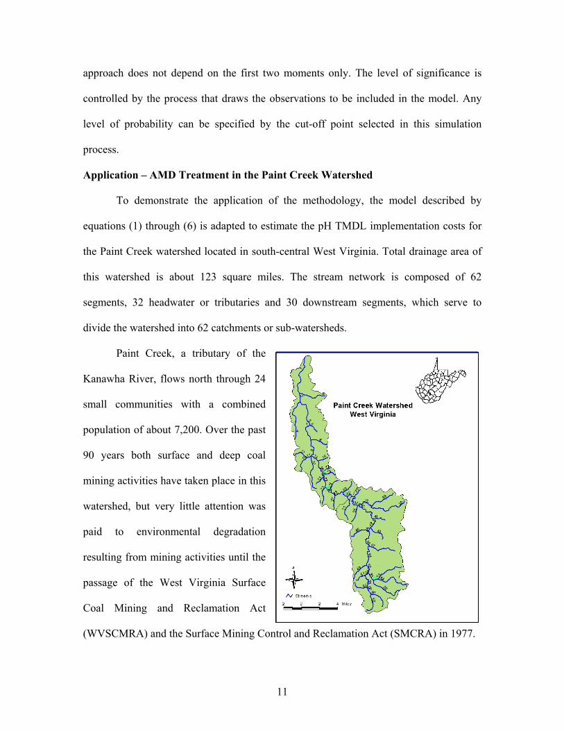
Application – AMD Treatment in the Paint Creek Watershed
To demonstrate the application of the methodology, the model described by
equations (1) through (6) is adapted to estimate the pH TMDL implementation costs for
the Paint Creek watershed located in south-central West Virginia. Total drainage area of
this watershed is about 123 square miles. The stream network is composed of 62
segments, 32 headwater or tributaries and 30 downstream segments, which serve to
divide the watershed into 62 catchments or sub-watersheds.
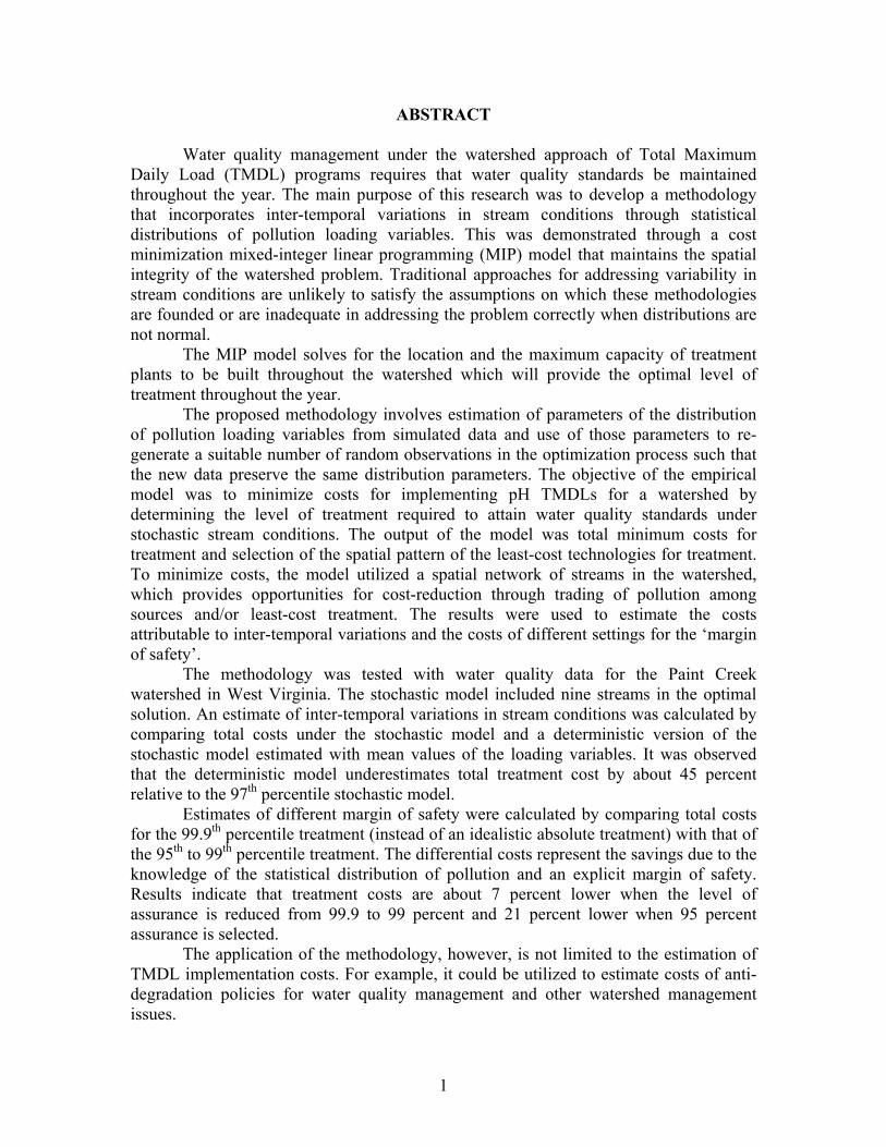
Paint Creek, a tributary of the
Kanawha River, flows north through 24
small communities with a combined
population of about 7,200. Over the past
90 years both surface and deep coal
mining activities have taken place in this
watershed, but very little attention was
paid to environmental degradation
resulting from mining activities until the
passage of the West Virginia Surface
Coal Mining and Reclamation Act
(WVSCMRA) and the Surface Mining Control and Reclamation Act (SMCRA) in 1977.
12
After coal extraction, mine openings and boreholes were abandoned allowing
surface water to seep into deep mines and react with sulfur and metal ions to form acidic
solutions. These acidic solutions flow out of the mine to the adjacent streams and
tributaries. The West Virginia Department of Environmental Protection (WVDEP) and
the Paint Creek Watershed Associations conducted water sampling at locations in both
the mainstream and tributary segments. The water in many locations was highly acidic
and far exceeded the West Virginia water quality standards which require waters to be
between pH 6.0 and 9.0.
Data Sources
Data for the empirical model of the Paint Creek watershed were obtained from
two major sources. Daily estimates of water flow and net acidity for all 62 stream
segments for a five year period (1992-96) were generated by the Total Acidic Mine
Drainage Loadings (TAMDL) model. TAMDL is a computer simulation model developed
by Stiles (2002) at the West Virginia Water Resources Institute, West Virginia University
to provide the analytical capabilities necessary to model in-stream concentrations and
reaction of the various constituents of acid mine drainage (AMD). The output of the
TAMDL model provided estimates of flow level and acid loadings in units of CaCO3
equivalent per year. TAMDL was applied as part of the development of the TMDL
allocations for the Paint Creek Watershed (USEPA, 2001b).
Detailed information on plant sizes and related fixed costs of operation for four
alkaline treatment technologies – soda ash (Na2CO3), caustic soda (NaOH), ammonia
(NH3), and hydrated lime (Ca(OH)2) – as well as per unit chemical reagent costs were
obtained from various studies conducted by Fletcher et al. (1991) and Phipps et al.
13
(1996). Soda ash based technologies can be applied to treat smaller amounts of acidity
with a plant capacity of 10 metric tons of CaCO3 equivalent acid per year. The other three
technologies can be applied to a wide range of flow-acidity conditions but may require
bigger capacity plants for high-flow-high-acidity waters. Treatment capacities of two
different plant sizes for caustic soda and ammonia and four different plant sizes for
hydrated lime were used. For caustic soda and ammonia, the derived capacities were 10
and 4,975 metric tons of CaCO3 equivalent per year, and for hydrated lime, the derived
capacities were 10, 199, 249, and 4,975 metric tons of CaCO3 equivalent acid per year
respectively. The model treated the various combinations as separate technologies – a
total of nine plant size, chemical technology combinations.
The Specific Model
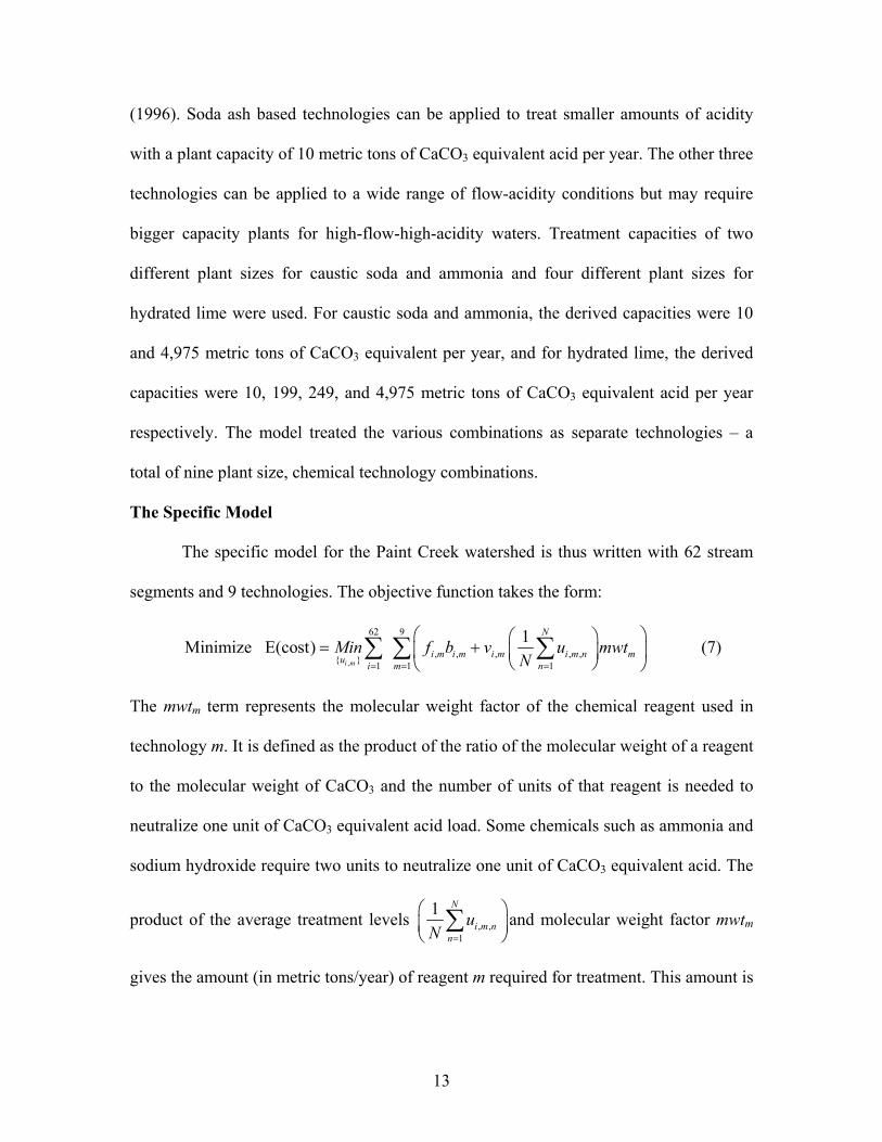
The specific model for the Paint Creek watershed is thus written with 62 stream
segments and 9 technologies. The objective function takes the form:
,
62 9
, , , , ,{ } 1 1 1
1Minimize E(cost) i m
N
i m i m i m i m n mu i m n
Min f b v u mwtN= = =
= +
∑ ∑ ∑ (7)
The mwtm term represents the molecular weight factor of the chemical reagent used in
technology m. It is defined as the product of the ratio of the molecular weight of a reagent
to the molecular weight of CaCO3 and the number of units of that reagent is needed to
neutralize one unit of CaCO3 equivalent acid load. Some chemicals such as ammonia and
sodium hydroxide require two units to neutralize one unit of CaCO3 equivalent acid. The
product of the average treatment levels , ,1
1 N
i m nn
uN =
∑ and molecular weight factor mwtm
gives the amount (in metric tons/year) of reagent m required for treatment. This amount is
14
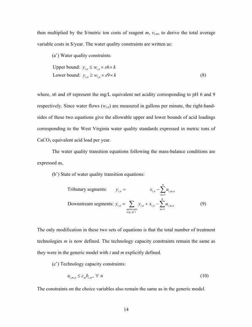
then multiplied by the $/metric ton costs of reagent m, vi,m, to derive the total average
variable costs in $/year. The water quality constraints are written as:
(a’) Water quality constraints:
, ,
, ,
Upper bound: 6Lower bound: 9
i n i n
i n i n
y w s ky w s k
≤ × ×
≥ × × (8)
where, s6 and s9 represent the mg/L equivalent net acidity corresponding to pH 6 and 9
respectively. Since water flows (wi,n) are measured in gallons per minute, the right-hand-
sides of these two equations give the allowable upper and lower bounds of acid loadings
corresponding to the West Virginia water quality standards expressed in metric tons of
CaCO3 equivalent acid load per year.
The water quality transition equations following the mass-balance conditions are
expressed as,
(b’) State of water quality transition equations:
9
, , , ,1
9
, , , , ,1
.
Tributary segments:
Downstream segments:
i n i n i m nm
i n i n i n i m nupstream mseg of i
y x u
y y x u
=
=
= −
= + −
∑
∑ ∑ (9)
The only modification in these two sets of equations is that the total number of treatment
technologies m is now defined. The technology capacity constraints remain the same as
they were in the generic model with i and m explicitly defined.
(c’) Technology capacity constraints:
, , , , i m n m i mu c b n≤ ∀ (10)
The constraints on the choice variables also remain the same as in the generic model.
15
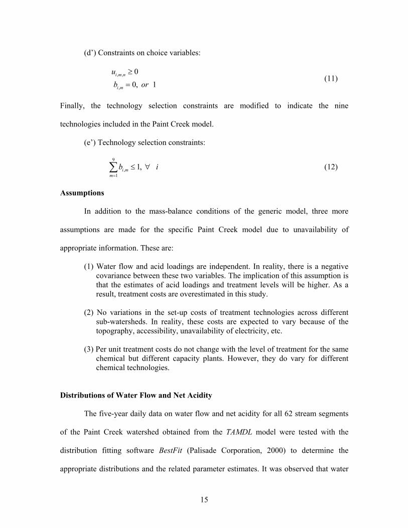
(d’) Constraints on choice variables:
, ,
,
0 0, 1
i m n
i m
ub or
≥
= (11)
Finally, the technology selection constraints are modified to indicate the nine
technologies included in the Paint Creek model.
(e’) Technology selection constraints:
9
,1
1,i mm
b i=
≤ ∀∑ (12)
Assumptions
In addition to the mass-balance conditions of the generic model, three more
assumptions are made for the specific Paint Creek model due to unavailability of
appropriate information. These are:
(1) Water flow and acid loadings are independent. In reality, there is a negative covariance between these two variables. The implication of this assumption is that the estimates of acid loadings and treatment levels will be higher. As a result, treatment costs are overestimated in this study.
(2) No variations in the set-up costs of treatment technologies across different
sub-watersheds. In reality, these costs are expected to vary because of the topography, accessibility, unavailability of electricity, etc.
(3) Per unit treatment costs do not change with the level of treatment for the same
chemical but different capacity plants. However, they do vary for different chemical technologies.
Distributions of Water Flow and Net Acidity
The five-year daily data on water flow and net acidity for all 62 stream segments
of the Paint Creek watershed obtained from the TAMDL model were tested with the
distribution fitting software BestFit (Palisade Corporation, 2000) to determine the
appropriate distributions and the related parameter estimates. It was observed that water
16
flow follows the lognormal distribution and net acidity follows the triangular distribution
for almost all segments. Some minor adjustments were made for those segments where
lognormal and triangular were not a perfect fit. Parameters of these distributions were
noted and used to re-generate these distributions through random draws in the
optimization model.
Two transformation functions linking a standard normal variable to the lognormal
parameters and a standard uniform variable to the triangular parameters were used in the
optimization programs to transform the normal and uniform variables directly available
in GAMS (Brook et al., 1998) as appropriate.
The triangular distribution is bounded by the minimum and maximum values
while the lognormal distribution is unbounded. The characteristic fat tail of the lognormal
probability density function (pdf) is asymptotic to the horizontal axis. The implication is
that the probability of obtaining an extremely large observation is never zero; random
observations drawn from the lognormal distribution will be arbitrarily large with some
positive probability. Acid loadings corresponding to these observations will also be large
and may go well beyond the treatment capacity of all feasible plants resulting in
infeasible model solutions. Even when the solution is feasible, the optimal solution will
include larger capacity treatment plants at a very high fixed cost and may significantly
overstate any observed or expected outcome.
To avoid this problem, an upper limit or treatment up to a selective percentile of
the distribution was used in the model, not the complete distribution. A large number of
observations (50,000) for the acid loadings for all 62 stream segments were drawn to
serve as the empirical distribution. These draws were then sorted in ascending order and
17
the 90th, 95th, 97th, 99th, and 99.9th percentile values noted. During the optimization
process, if any random draw resulted in a value greater than the appropriate percentile
values for a given run, they were censored appropriately. The model was run with 700
sample observations for each of the percentile levels of treatment noted above and
treatment levels, fixed, and variable costs compared.
Methodology
The MIP model for the Paint Creek watershed was estimated using the CPlex
solver available with the GAMS software. The lognormal and triangular parameters
obtained from the BestFit software were used in the GAMS program and transformation
functions were used to link these parameters with draws from standard normal and
standard uniform variables to re-generate the distributions of lognormal water flow and
triangular net acidity. The simulated flow and acidity data were then used to calculate the
acid loadings included in the optimization model. All stream segments were assigned the
same randomly drawn value in a particular draw to reflect the high spatial autocorrelation
between flows and loadings at a specified point in time. The implication of this drawing
process is that any change in the upstream loadings will affect the downstream loadings
proportionately and is in accordance with the mass balance approach used in the linear
approximation. During the optimization process, a suitable number of sample
observations for lognormally distributed water flow and triangularly distributed net
acidity were drawn and corresponding acid loadings calculated and checked against those
percentile values. Loadings that exhibit values greater than a specific percentile value
were replaced by that percentile value. The GAMS/Cplex solvers used dual simplex and
branch-and-bound algorithms.
18
Results
Increasing the percentile values implies usage of more area from the positively
skewed tail of the lognormal distribution. This increases the probability of encountering
more extreme observations in the optimization process. For the present problem, these
more extreme values simply mean higher levels and costs of treatment. If a larger plant is
required to treat the higher load, this may require installation of higher capacity treatment
plants as well. This issue is investigated for a fixed sample size of 700 observations and
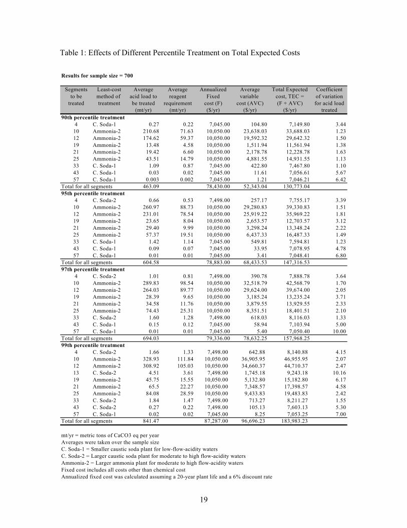
for variable levels of treatment. The results are presented in Table 1.
Summary results in Table 1 suggest that total expected costs (TEC) of treatment
increase with increases in the percentile of loads fully treated. The increase in the cost is
primarily due to the higher amount of acid treatment which sometimes requires higher
capacity treatment plants. Smaller caustic soda plants were sufficient to meet the
treatment requirements for the 90th percentile treatment. When the required level of
treatment increases from the 90th to the 95th percentile, smaller caustic soda plant
originally selected for stream segment 4 is no longer sufficient. For treating the 97th
percentile treatment, segments 4 and 33 both require larger caustic soda plants. For even
higher 99th percentile treatment level, stream segments 4, 33, 43 and a new segment 13
which do not require any treatment previously for lower bounds, also need the larger
caustic soda plants. This increased capacity simply translates to higher fixed costs.
With 700 sample observations, the activity matrix had 520,862 rows and 434,558
columns with 1,736,417 non-zero elements. The proportion of non-zero elements was
7.67×10– 6. The CPlex solver used 153,969 iterations to achieve the optimum solution and
required 1.7 GB virtual memory and 21 minutes CPU time with a P-III 550.
19
Table 1: Effects of Different Percentile Treatment on Total Expected Costs
Results for sample size = 700
Segments Least-cost Average Average Annualized Average Total Expected Coefficientto be method of acid load to reagent Fixed variable cost, TEC = of variation
treated treatment be treated requirement cost (F) cost (AVC) (F + AVC) for acid load(mt/yr) (mt/yr) ($/yr) ($/yr) ($/yr) treated
90th percentile treatment4 C. Soda-1 0.27 0.22 7,045.00 104.80 7,149.80 3.44
10 Ammonia-2 210.68 71.63 10,050.00 23,638.03 33,688.03 1.2312 Ammonia-2 174.62 59.37 10,050.00 19,592.32 29,642.32 1.5019 Ammonia-2 13.48 4.58 10,050.00 1,511.94 11,561.94 1.3821 Ammonia-2 19.42 6.60 10,050.00 2,178.78 12,228.78 1.6325 Ammonia-2 43.51 14.79 10,050.00 4,881.55 14,931.55 1.1333 C. Soda-1 1.09 0.87 7,045.00 422.80 7,467.80 1.1043 C. Soda-1 0.03 0.02 7,045.00 11.61 7,056.61 5.6757 C. Soda-1 0.003 0.002 7,045.00 1.21 7,046.21 6.42
Total for all segments 463.09 78,430.00 52,343.04 130,773.0495th percentile treatment
4 C. Soda-2 0.66 0.53 7,498.00 257.17 7,755.17 3.3910 Ammonia-2 260.97 88.73 10,050.00 29,280.83 39,330.83 1.5112 Ammonia-2 231.01 78.54 10,050.00 25,919.22 35,969.22 1.8119 Ammonia-2 23.65 8.04 10,050.00 2,653.57 12,703.57 3.1221 Ammonia-2 29.40 9.99 10,050.00 3,298.24 13,348.24 2.2225 Ammonia-2 57.37 19.51 10,050.00 6,437.33 16,487.33 1.4933 C. Soda-1 1.42 1.14 7,045.00 549.81 7,594.81 1.2343 C. Soda-1 0.09 0.07 7,045.00 33.95 7,078.95 4.7857 C. Soda-1 0.01 0.01 7,045.00 3.41 7,048.41 6.80
Total for all segments 604.58 78,883.00 68,433.53 147,316.5397th percentile treatment
4 C. Soda-2 1.01 0.81 7,498.00 390.78 7,888.78 3.6410 Ammonia-2 289.83 98.54 10,050.00 32,518.79 42,568.79 1.7012 Ammonia-2 264.03 89.77 10,050.00 29,624.00 39,674.00 2.0519 Ammonia-2 28.39 9.65 10,050.00 3,185.24 13,235.24 3.7121 Ammonia-2 34.58 11.76 10,050.00 3,879.55 13,929.55 2.3325 Ammonia-2 74.43 25.31 10,050.00 8,351.51 18,401.51 2.1033 C. Soda-2 1.60 1.28 7,498.00 618.03 8,116.03 1.3343 C. Soda-1 0.15 0.12 7,045.00 58.94 7,103.94 5.0057 C. Soda-1 0.01 0.01 7,045.00 5.40 7,050.40 10.00
Total for all segments 694.03 79,336.00 78,632.25 157,968.2599th percentile treatment
4 C. Soda-2 1.66 1.33 7,498.00 642.88 8,140.88 4.1510 Ammonia-2 328.93 111.84 10,050.00 36,905.95 46,955.95 2.0712 Ammonia-2 308.92 105.03 10,050.00 34,660.37 44,710.37 2.4713 C. Soda-2 4.51 3.61 7,498.00 1,745.18 9,243.18 10.1619 Ammonia-2 45.75 15.55 10,050.00 5,132.80 15,182.80 6.1721 Ammonia-2 65.5 22.27 10,050.00 7,348.57 17,398.57 4.5825 Ammonia-2 84.08 28.59 10,050.00 9,433.83 19,483.83 2.4233 C. Soda-2 1.84 1.47 7,498.00 713.27 8,211.27 1.5543 C. Soda-2 0.27 0.22 7,498.00 105.13 7,603.13 5.3057 C. Soda-1 0.02 0.02 7,045.00 8.25 7,053.25 7.00
Total for all segments 841.47 87,287.00 96,696.23 183,983.23
mt/yr = metric tons of CaCO3 eq per yearAverages were taken over the sample sizeC. Soda-1 = Smaller caustic soda plant for low-flow-acidity watersC. Soda-2 = Larger caustic soda plant for moderate to high flow-acidity watersAmmonia-2 = Larger ammonia plant for moderate to high flow-acidity watersFixed cost includes all costs other than chemical costAnnualized fixed cost was calculated assuming a 20-year plant life and a 6% discount rate
20
Margin of Safety (MOS)
The TMDL guidelines suggest an ad hoc adjustment to the end-points of
allowable loads in determining MOS inclusive load allocations for point and non-point
sources. This approach sidesteps the requirements of examining the actual statistical
distributions of pollutant loadings. Implementation of such TMDLs requires building
larger capacity treatment plants at higher costs. If the true distributions of loadings were
known, allocations would have been lower, requiring lower implementation costs. The
different costs of these two scenarios would then be interpreted as the savings due to the
knowledge of the true MOS.
Since the distributions of polluting variables are known in this study, arbitrary
adjustments to the end-points of allowable loads are not necessary to get an estimate of
savings due to the knowledge of MOS. Rather, it is possible to determine the exact
amount of treatment to be carried out or the level of plant capacity to be built to achieve a
target level of assurance. This approach is followed in the present study to estimate the
savings due to the knowledge of MOS corresponding to different levels of assurance.
Since the 100th percentile treatment of acid load is empirically impossible in the present
approach due to the presence of the asymptotic tail, the maximum attainable level of
safety was assumed to be with the 99.9th percentile treatment. Costs associated with this
level of assurance were compared with that of a more pragmatic and attainable goal of
the 95th to 99th percentile treatment. The differential costs provide the estimates of
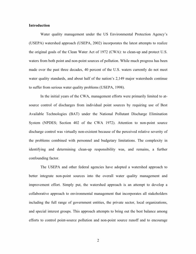
savings for the knowledge of MOS. The results are presented in Figure 1.
21
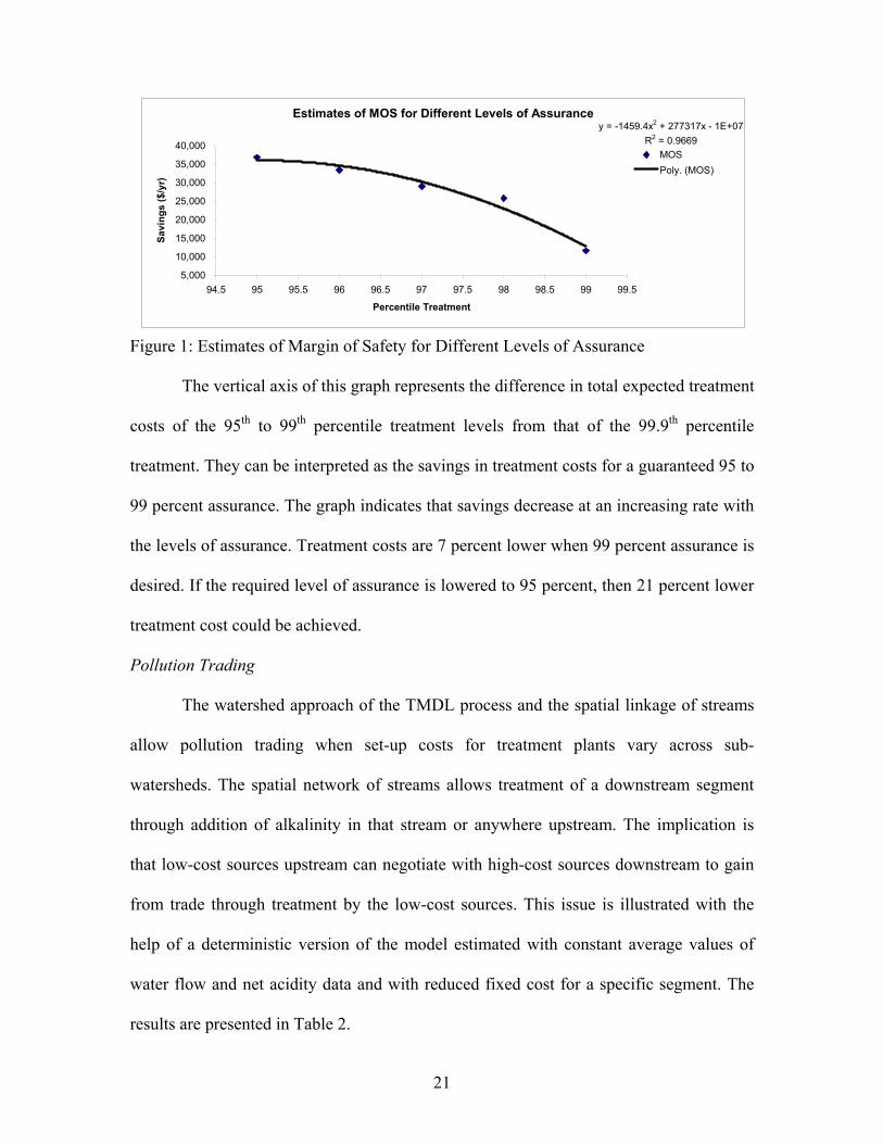
Figure 1: Estimates of Margin of Safety for Different Levels of Assurance
The vertical axis of this graph represents the difference in total expected treatment
costs of the 95th to 99th percentile treatment levels from that of the 99.9th percentile
treatment. They can be interpreted as the savings in treatment costs for a guaranteed 95 to
99 percent assurance. The graph indicates that savings decrease at an increasing rate with
the levels of assurance. Treatment costs are 7 percent lower when 99 percent assurance is
desired. If the required level of assurance is lowered to 95 percent, then 21 percent lower
treatment cost could be achieved.
Pollution Trading
The watershed approach of the TMDL process and the spatial linkage of streams
allow pollution trading when set-up costs for treatment plants vary across sub-
watersheds. The spatial network of streams allows treatment of a downstream segment
through addition of alkalinity in that stream or anywhere upstream. The implication is
that low-cost sources upstream can negotiate with high-cost sources downstream to gain
from trade through treatment by the low-cost sources. This issue is illustrated with the
help of a deterministic version of the model estimated with constant average values of
water flow and net acidity data and with reduced fixed cost for a specific segment. The
results are presented in Table 2.
Estimates of MOS for Different Levels of Assurancey = -1459.4x2 + 277317x - 1E+07
R2 = 0.9669
5,000
10,000
15,000
20,000
25,000
30,000
35,000
40,000
94.5 95 95.5 96 96.5 97 97.5 98 98.5 99 99.5
Percentile Treatment
Savi
ngs
($/y
r)MOSPoly. (MOS)
22
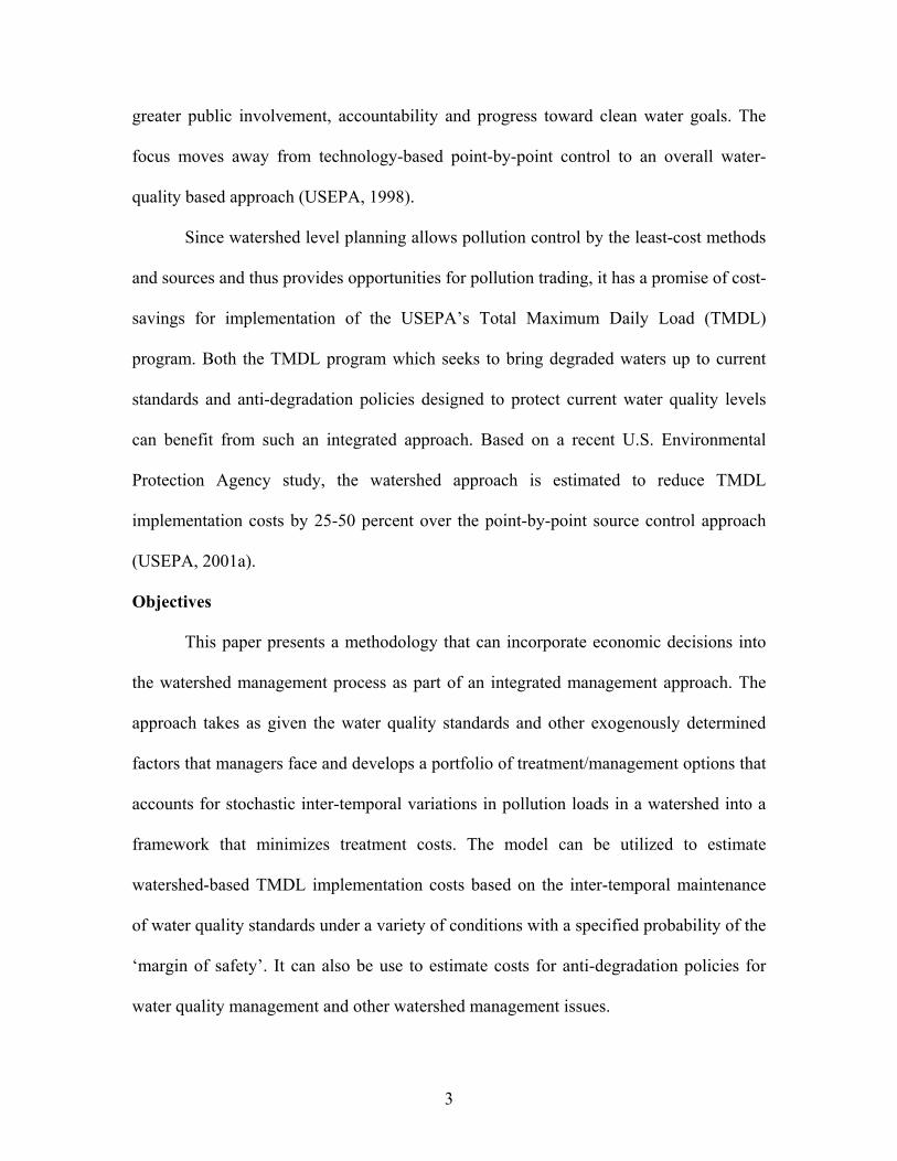
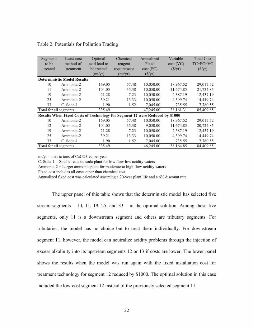
Table 2: Potentials for Pollution Trading
The upper panel of this table shows that the deterministic model has selected five
stream segments – 10, 11, 19, 25, and 33 – in the optimal solution. Among these five
segments, only 11 is a downstream segment and others are tributary segments. For
tributaries, the model has no choice but to treat them individually. For downstream
segment 11, however, the model can neutralize acidity problems through the injection of
excess alkalinity into its upstream segments 12 or 13 if costs are lower. The lower panel
shows the results when the model was run again with the fixed installation cost for
treatment technology for segment 12 reduced by $1000. The optimal solution in this case
included the low-cost segment 12 instead of the previously selected segment 11.
Segments Least-cost Optimal Chemical Annualized Variable Total Costto be method of acid load to reagent Fixed cost (VC) TC=FC+VC
treated treatment be treated requirement cost (FC) ($/yr) ($/yr)(mt/yr) (mt/yr) ($/yr)
Deterministic Model Results10 Ammonia-2 169.05 57.48 10,050.00 18,967.52 29,017.52 11 Ammonia-2 104.05 35.38 10,050.00 11,674.85 21,724.85 19 Ammonia-2 21.28 7.23 10,050.00 2,387.19 12,437.19 25 Ammonia-2 39.21 13.33 10,050.00 4,399.74 14,449.74 33 C. Soda-1 1.90 1.52 7,045.00 735.55 7,780.55
Total for all segments 335.49 47,245.00 38,161.31 85,409.85 Results When Fixed Costs of Technology for Segment 12 were Reduced by $1000
10 Ammonia-2 169.05 57.48 10,050.00 18,967.52 29,017.52 12 Ammonia-2 104.05 35.38 9,050.00 11,674.85 20,724.85 19 Ammonia-2 21.28 7.23 10,050.00 2,387.19 12,437.19 25 Ammonia-2 39.21 13.33 10,050.00 4,399.74 14,449.74 33 C. Soda-1 1.90 1.52 7,045.00 735.55 7,780.55
Total for all segments 335.49 46,245.00 38,164.85 84,409.85
mt/yr = metric tons of CaCO3 eq per yearC. Soda-1 = Smaller caustic soda plant for low flow-low acidity watersAmmonia-2 = Larger ammonia plant for moderate to high flow-acidity watersFixed cost includes all costs other than chemical costAnnualized fixed cost was calculated assuming a 20-year plant life and a 6% discount rate
23
The implication of this exercise is that if the sources in sub-watershed 11 have
higher costs for treatment, they can negotiate with the lower cost sources in sub-
watersheds 12 or 13 to come up with a cheaper cost alternative strategy. Sources in sub-
watershed 11 would be willing to offer any price lower than $21,724.85 for this clean-up
activity while sources in sub-watershed 12 or 13 would be willing to take any price above
$20,724.85. Both parties will be benefited from this trade and a Pareto optimal
improvement in the solution will be achieved.
Estimates of Inter-temporal Variations
The effect of inter-temporal variations was investigated by comparing the results
of the stochastic model with that of the deterministic model. The difference in the total
minimized costs indicates the extent of underestimation in treatment costs if variability in
stream conditions is ignored.
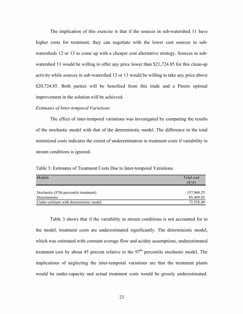
Table 3: Estimates of Treatment Costs Due to Inter-temporal Variations
Table 3 shows that if the variability in stream conditions is not accounted for in
the model, treatment costs are underestimated significantly. The deterministic model,
which was estimated with constant average flow and acidity assumptions, underestimated
treatment cost by about 45 percent relative to the 97th percentile stochastic model. The
implications of neglecting the inter-temporal variations are that the treatment plants
would be under-capacity and actual treatment costs would be grossly underestimated.
Models Total cost($/yr)
Stochastic (97th percentile treatment) 157,968.25Deterministic 85,409.85Under-estimate with deterministic model 72,558.40
24
Alternatively, the treatment levels would be far from sufficient a significant proportion of
the time.
Conclusions
In this paper, a stochastic mixed-integer programming methodology is presented
to address the inter-temporal variations in pollution loadings in the stream network of a
spatially integrated watershed. Traditional programming approaches are unsatisfactory
for the assumptions on which they are based or are inadequate when distributions are not
normal. The proposed methodology makes no a priori assumptions, rather estimates
distribution parameters from simulated data to use in the optimization process. The
methodology is applied to estimate pH TMDL implementation costs for the Paint Creek
watershed in West Virginia. The empirical model provided information on which stream
segments should be treated, the method of treatment, the levels of treatment for which
investments need to be made, and the estimated cost. The model also indicates the trade-
off between treatment plant capacities and the level of assurance or margin of safety. The
approach allows a clear calculation of the cost of increased margins of safety and should
provide input to stimulate discussion of potential trade-offs possible within a watershed
framework.
A deterministic version of the model is also estimated with average levels of
water flow and net acidity for the Paint Creek streams. The optimal solution included
four tributary segments and one downstream segment for treatment. These results are
compared with that for another run of the deterministic model which included a reduced
fixed set-up costs for a specific upstream segment to demonstrate the potentials for
25
pollution trading. Results show that when abatement costs differ among sources, it is
possible to gain from trade through treatment by lower cost sources.
A comparison of stochastic and deterministic model results indicates that when
inter-temporal variability in stream conditions is ignored, the treatment cost is
underestimated significantly; the difference between the deterministic and the 97th
percentile treatment with the stochastic model is about 45 percent.
26
References
Arbabi, M. and J. Elzinga (1975): A General Linear Approach to Stream Water Quality Modeling, Water Resources Research, 11(2), 191-196.
Benjamin, J.R. and C.A. Cornell (1970): Probability, Statistics, and Decision for Civil Engineers, McGraw-Hill, New York.
Brook, A., D. Kendrick, A. Meeraus, and R. Raman (1998): GAMS A User’s Guide, GAMS Development Corporation, Washington, DC.
Burges, S.J. and D.P. Lettenmaier (1975): Probabilistic Methods in Stream Quality Management, Water Resources Bulletin, 11(1), 115-130.
Burn, D.H. and E.A. McBean (1985): Optimization Modeling of Water Quality in an Uncertain Environment, Water Resources Research, 21(7), 934-940.
Charnes, A. and W.W. Cooper (1959): Chance-constrained Programming, Management Science, Vol. 6, October 1959, 73-79.
Charnes, A. and W.W. Cooper (1962): Chance Constraints and Normal Deviates, Journal of the American Statistical Association, 57(297), March 1962, 134-148.
Charnes, A. and W.W. Cooper (1963): Deterministic Equivalents for Optimizing and Satisficing Under Chance Constraints, Operations Research, 11(1), 18-39.
Fletcher, J.J., T.T. Phipps, and J.G. Skousen (1991): Cost Analysis for Treating Acid Mine Drainage From Coal Mines in the U.S., Paper presented at the Second International Conference on the Abatement of Acidic Drainage, September 16-18, 1991, Montreal.
GAMS Development Corporation (2001): GAMS – The Solver Manuals, Washington, DC.
Liebman, J.C. and W.R.Lynn (1966): The Optimal Allocation of Stream Dissolved Oxygen, Water Resources Research, 2(3), 581-91.
Lohani, B.N. and N.C. Thanh (1978): Stochastic Programming Model for Water Quality Management in a River, Journal of Water Pollution Control Federation, 50(9), 2175-2182.
Loucks, D.P., C.S. Revelle and W.R. Lynn (1967): Linear Programming Models for Water Pollution Control, Management Science, 14(4), B166-B181.
Palisade Corporation (2000): Guide to Using BestFit Distribution Fitting for Windows, Version 4, April 2000, Newfield, NY, USA. http://www.palisade.com
Phipps, T.T., J.J. Fletcher, and J.G. Skousen (1991): A Methodology for Evaluating the Costs of Alternative AMD Treatment Systems, Paper presented at the Twelfth Annual West Virginia Surface Mine Drainage Task Force Symposium, Morgantown, West Virginia, April 3-4, 1991.
Phipps, T.T., J.J. Fletcher, and J.G. Skousen (1992): Draft Final Report, Economics Section, NMLRC Project WV-10 1990-91. College of Agriculture and Forestry, West Virginia University, Morgantown, West Virginia.
Phipps, T.T., J.J. Fletcher, and F.G. Skousen (1996): Costs for Chemical Treatment of AMD, Chapter 18, in Skousen, J.G. and P.F. Ziemkiewicz (compiled): Acid Mine Drainage: Control and Treatment, Second Edition, West Virginia University and the National Mine Land Reclamation Center, Morgantown, West Virginia.
27
Revelle, C.S., D.P. Loucks and W.R. Lynn (1968): Linear Programming Applied to Water Quality Management, Water Resources Research, 4(1), 1-9.
Sengupta, J.K. (1970): Stochastic Linear Programming With Chance Constraints, International Economic Review, 11(1), 101-116.
Shortle, J.S. (1990): The Allocative Efficiency Implications of Water Pollution Abatement Cost Comparisons, Water Resources Research, 26(5), 793-97.
Stiles, J.M. (2002): TMDL Model Development for Acidic Mine Drainage, Water Resources Update, Universities Council on Water Resources, 4543 Faner Hall, Southern Illinois University at Carbondale, Carbondale, IL 62901-4526.
Tietenberg, T. (1985): Emissions Trading: An Exercise in Reforming Pollution Policy, Resources for the Future, Washington, DC.
U.S. Environmental Protection Agency (1998): Clean Water Action Plan: Restoring and Protecting America’s Waters, US Government Printing Office, Washington, DC.
U.S. Environmental Protection Agency (1999a): Draft Guidance for Water Quality-based Decision: The TMDL Process, Second Edition, Washington, DC.
U.S. Environmental Protection Agency (2001a): The National Costs of the Total Maximum Daily Load Program (Draft Report), Washington, DC.
U.S. Environmental Protection Agency (2001b): The National Costs to Develop TMDLs (Draft Report), Support Document # 1, Washington, DC.
U.S. Environmental Protection Agency (2001c): The National Costs to Implement TMDLs (Draft Report), Support Document # 2, Washington, DC.
U.S. Environmental Protection Agency (2001d): Paint Creek, WV pH, aluminum, iron, and manganese TMDL, EPA Region 3, Philadelphia, PA
http://www.epa.gov/reg3wapd/tmdl/pdf/paint_creek/finalreport.pdf Zhu, M., D.B. Taylor, S.C. Sarin, and R.A. Kramer (1994): Chance Constrained
Programming Model for Risk-Based Economic and Policy Analysis of Soil Conservation, Agricultural and Resource Economics Review, 23(1), 58-65.