Embed Size (px)
Citation preview

Stream Restoration on Soldier Creek
Jared Neil Erickson
A Project Report submitted to the faculty of Brigham Young University
in partial fulfillment of the requirements for the degree of
Master of Science
Rollin H. Hotchkiss, Chair Jordan Nielson
E. James Nelson Daniel P. Ames
Department of Civil and Environmental Engineering
Brigham Young University
March 2013
Copyright © 2013 Jared Erickson
All Rights Reserved
ABSTRACT
Stream Restoration on Soldier Creek
Jared Neil Erickson Department of Civil and Environmental Engineering, BYU
Master of Science
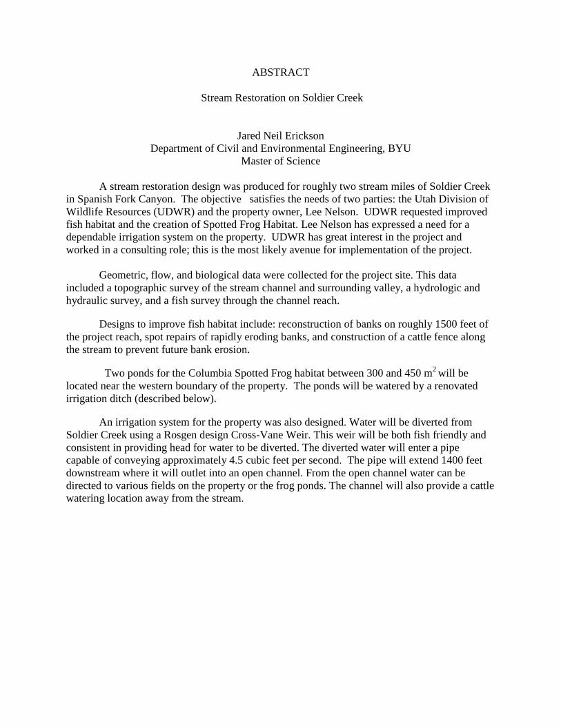
A stream restoration design was produced for roughly two stream miles of Soldier Creek in Spanish Fork Canyon. The objective satisfies the needs of two parties: the Utah Division of Wildlife Resources (UDWR) and the property owner, Lee Nelson. UDWR requested improved fish habitat and the creation of Spotted Frog Habitat. Lee Nelson has expressed a need for a dependable irrigation system on the property. UDWR has great interest in the project and worked in a consulting role; this is the most likely avenue for implementation of the project.
Geometric, flow, and biological data were collected for the project site. This data
included a topographic survey of the stream channel and surrounding valley, a hydrologic and hydraulic survey, and a fish survey through the channel reach.
Designs to improve fish habitat include: reconstruction of banks on roughly 1500 feet of the project reach, spot repairs of rapidly eroding banks, and construction of a cattle fence along the stream to prevent future bank erosion.
Two ponds for the Columbia Spotted Frog habitat between 300 and 450 m2 will be located near the western boundary of the property. The ponds will be watered by a renovated irrigation ditch (described below).
An irrigation system for the property was also designed. Water will be diverted from Soldier Creek using a Rosgen design Cross-Vane Weir. This weir will be both fish friendly and consistent in providing head for water to be diverted. The diverted water will enter a pipe capable of conveying approximately 4.5 cubic feet per second. The pipe will extend 1400 feet downstream where it will outlet into an open channel. From the open channel water can be directed to various fields on the property or the frog ponds. The channel will also provide a cattle watering location away from the stream.


ACKNOWLEDGEMENTS
First I need to acknowledge Jeremy Payne, my partner in putting this project together. I
couldn’t have asked for someone better to work with and I’m grateful to be able to leave this
work in his capable hands.
I also want to acknowledge the Spring 2012 CEEn 635 class for all the work that they put
into the project. They were instrumental in assisting with the data collection on Soldier Creek.
Each member of the class had a hand in the Data Collection section of this report.
Jordan Nielson has been a mentor of mine for a long time leading up to the project and it
was a blessing to have him as an official mentor to this project. He has patiently taught me a
great deal over the past couple of years and has been invaluable in developing me professionally
and personally.
My final acknowledgment is for Dr. Rollin H. Hotchkiss. He has been a true teacher. He
has always demanded that I bring my best and has pushed me to be better than I thought that I
could. I am grateful that he chose to work with me and for seeing in me the potential to be a
great engineer.


v
TABLE OF CONTENTS
LIST OF FIGURES ..................................................................................................................... xi
1 Introduction ........................................................................................................................... 1
1.1 Area ................................................................................................................................. 1
1.1.1 Project Location .......................................................................................................... 1
1.1.2 Vegetation ................................................................................................................... 3
1.1.3 History ......................................................................................................................... 4
1.1.4 Beavers ........................................................................................................................ 7
1.2 Land Owner .................................................................................................................... 7
1.3 Cooperative Agency ....................................................................................................... 8
2 Data Collection .................................................................................................................... 11
2.1 Channel Survey ............................................................................................................. 11
2.2 Stream Classification .................................................................................................... 13
2.3 Valley and Channel Survey .......................................................................................... 14
2.4 Three Sections ............................................................................................................... 16
2.5 HEC-RAS Model .......................................................................................................... 19
2.6 HQI ............................................................................................................................... 23
2.7 Fish Survey ................................................................................................................... 24
3 Reference Reach .................................................................................................................. 26
4 Restoration Design .............................................................................................................. 29
4.1 Objectives ..................................................................................................................... 29
4.2 Improve Fish Habitat .................................................................................................... 29
4.2.1 Reconstruction of Banks near the House .................................................................. 29
4.2.2 Channel Modifications/ Considerations .................................................................... 32

vi
4.2.3 Non-Treated Eroding Banks ..................................................................................... 45
4.2.4 Cattle Grazing/Passive Restoration ........................................................................... 47
4.3 Construct Habitat Ponds for Endanger Spotted Frog .................................................... 49
4.4 Build a Dependable Diversion ...................................................................................... 51
4.4.1 Old Diversion ............................................................................................................ 52
4.4.2 Proposed Design ....................................................................................................... 53
4.5 Time to Complete/ Project Phasing .............................................................................. 59
4.6 Cost Estimates ............................................................................................................... 60
5 Appendix 1 Data Collection: .............................................................................................. 63
5.1 Soldier Creek ................................................................. Error! Bookmark not defined.
5.2 Hydraulic Survey .......................................................................................................... 63
5.2.1 Determining Slope, Discharge, and Manning’s “n” ................................................. 63
5.2.2 Sediment Analysis .................................................................................................... 70
5.2.3 Bankfull Indices ........................................................................................................ 72
5.2.4 Stream Profiles .......................................................................................................... 76
5.2.5 Stream Stats .............................................................................................................. 79
5.2.6 HQI ........................................................................................................................... 80
5.3 Salina Creek .................................................................................................................. 84
6 Appendix 2 Restoration Design ......................................................................................... 99
6.1 Frog Ponds .................................................................................................................... 99
6.1.1 Pond #1 ................................................................................................................... 100
6.1.2 Pond #2 ................................................................................................................... 101
6.2 Diversion ..................................................................................................................... 102
6.2.1 Diversion Structure ................................................................................................. 102
6.3 Pump ........................................................................................................................... 102

vii
6.4 Pipe ............................................................................................................................. 103
6.5 Channel ....................................................................................................................... 107
6.6 Cost Estimates ............................................................................................................. 109
7 Works Cited ....................................................................................................................... 111

viii
LIST OF TABLES
Table 1 : Hydraulic Measurements (Taken May 16, 2012) ...................................................11
Table 2: Bankfull Measurements ...........................................................................................12
Table 3: Bankfull Discharge ..................................................................................................12
Table 4: Predicted Fish Pounds Per Acre ..............................................................................24
Table 5: Fish Species Count ..................................................................................................25
Table 6: Fish Species Average Weight, and Length ..............................................................25
Table 7: Stream Dimensions and Fish Abundance Metrics ...................................................25
Table 8: Equations for Calculating Vane Length ..................................................................36
Table 9: Equations for Calculating Vane Spacing .................................................................36
Table 10: J-Hook Vane Parameters .......................................................................................36
Table 11: Minimum Rock Size Calculation...........................................................................37
Table 12: Location 2 Structure Dimensions ..........................................................................39
Table 13: Estimated Relic Channel Dimensions ...................................................................42
Table 14: Channel Dimensions ..............................................................................................59
Table 15: Time Estimate of Work to be completed ...............................................................59
Table 16: Potential Phase 1: Berm Removal .........................................................................60
Table 17: Potential Phase 2: Remainder of Project ...............................................................60
Table 18: Stream Improvement Material Costs .....................................................................61
Table 19: Diversion Material Costs .......................................................................................61
Table 20: Equipment Rental Costs ........................................................................................62
Table 21: Labor Costs ............................................................................................................62
Table 22: Total Costs .............................................................................................................62
Table 23. Velocity Measurements and Calculations..............................................................64

ix
Table 24. Slope Measurements ..............................................................................................65
Table 25. Slope Calculations .................................................................................................65
Table 26. Area and Discharge Calculations ...........................................................................66
Table 27. Wetted Perimeter Calculations ..............................................................................68
Table 28. Manning's Roughness Calculations .......................................................................69
Table 29. Bottom Shear Stress Calculations ..........................................................................69
Table 30: Wolman Pebble Count ...........................................................................................71
Table 31: Surficial Sediment Sample, Table of Percentiles ..................................................72
Table 32: Bankfull Indices Indicators (NEH 654) .................................................................73
Table 33: Bankfull Indices Values .........................................................................................75
Table 34: Water Quality Measurements ................................................................................82
Table 35: Count of Benthic Macroinvertebrates ....................................................................82
Table 36: Cover, Width, and Eroding Banks .........................................................................83
Table 37: Late Summer and Annual Flow .............................................................................83
Table 38: Predicted Fish Pounds Per Acre ............................................................................84
Table 39: Comparison Chart Between Salina Creek and Soldier Creek ...............................85
Table 40: Channel Dimension Ratios ....................................................................................86
Table 41: Channel Pattern Ratios ..........................................................................................86
Table 42: Channel Profile Ratios ...........................................................................................87
Table 43: Sediment Sample Salina Creek ..............................................................................88

x

xi
LIST OF FIGURES
Figure 1: Deliniated Watershed for Soldier Creek ................................................................2
Figure 2: Soldier Creek Project Site ......................................................................................2
Figure 3: Lower Section of Project Site .................................................................................3
Figure 4: Upper Section of Project Site .................................................................................3
Figure 5: Old Denver and Rio Grande Western Steam Locomotive, Thistle Utah 1951 (Tempus, World) ..........................................................................4
Figure 6: Project Area Flooding After Landslide (Thistle, Utah Landslide, 1983) ...............5
Figure 7: Beaver Dam upstream of new diversion. ...............................................................7
Figure 8: Surveying the monument on an adjacent mountain top. ........................................Error! Bookmark not defined.
Figure 9: Distribution of both GPS and DEM data points along Soldier Creek. ...................15
Figure 10: TIN produced from GPS and DEM data points. ..................................................16
Figure 11: Lower, Middle, and Upper Sections .....................................................................16
Figure 12: Lower Section.......................................................................................................17
Figure 13: Middle Section .....................................................................................................18
Figure 14: Upper Section .......................................................................................................19
Figure 15: Cross Sections created in HEC-RAS....................................................................20
Figure 16: HEC-RAS Lower Section Cross Section .............................................................21
Figure 17: HEC-RAS Middle Section Cross Section ............................................................21
Figure 18: HEC-RAS Upper Section Cross Section ..............................................................22
Figure 19: HQI Sampling Locations ......................................................................................24
Figure 20: Regional Curve .....................................................................................................27
Figure 21: Salina Creek .........................................................................................................28

xii
Figure 22: Berms to Be Removed ..........................................................................................30
Figure 23: Excavation Cross Section .....................................................................................31
Figure 24: Reference Reach Sample Cross Section ...............................................................32
Figure 25: Locations of High Erosion Sites ...........................................................................32
Figure 26: Bare Wall of Location 1. ......................................................................................33
Figure 27: J-Hook Vanes. Flow going right to left. ...............................................................34
Figure 28: Design Parameters for J-Hook Vanes ..................................................................35
Figure 29: Cross Sectional View of a Bankfull Bench. .........................................................38
Figure 30: Exposed Bare Wall at Location 2. ........................................................................38
Figure 31: Location 2 Design ................................................................................................40
Figure 32: Exposed Hill Side at Location 3. ..........................................................................41
Figure 33: Newly Designed Channel at Location 3. ..............................................................42
Figure 34: Upstream Cross Section .......................................................................................Error! Bookmark not defined.
Figure 35: Downstream Cross Section ..................................................................................Error! Bookmark not defined.
Figure 36: Old Diversion .......................................................................................................44
Figure 37: Sensitive Beaver Areas .........................................................................................45
Figure 38: Non-Treated Eroding Banks .................................................................................45
Figure 39: Location 1 Eroding Banks ....................................................................................46
Figure 40: Location 2 Eroding Bank .....................................................................................46
Figure 42: Fence Location .....................................................................................................47
Figure 43: Fence Design ........................................................................................................48
Figure 44: H-brace Design .....................................................................................................49
Figure 45: Columbia Spotted Frog ........................................................................................50
Figure 46: Frog Ponds ............................................................................................................51

xiii
Figure 47: Old Diversion Structure........................................................................................52
Figure 48: Old Diversion and Irrigated Fields .......................................................................52
Figure 49: Proposed Diversion and Fields to Be Irrigated ....................................................53
Figure 50: Diversion Structure (flow from left to right) ........................................................54
Figure 51: Cross Vane Diversion Structure- Clear Creek in Sun Valley, Idaho ...................55
Figure 52: Cross Vane Diversion Structure - Clear Creek in Sun Valley, Idaho ..................56
Figure 53: Augmented Cross Vane Structure - East Fork Piedra River, CO .........................56
Figure 54: Head Gate Structure .............................................................................................Error! Bookmark not defined.
Figure 55: Diversion Head Gate - Clear Creek in Sun Valley, Idaho ....................................57
Figure 56: Pipeline Profile .....................................................................................................58
Figure 57: Channel Depiction ................................................................................................59
Figure 58, Cross section with area calculation divisions .......................................................67
Figure 59: Wolman Pebble Count Particle Size Distribution ................................................70
Figure 60: Surficial Sediment Sample Locations ..................................................................71
Figure 61: Surficial Sediment Sample, Particle Size Distribution .........................................72
Figure 62: Bankfull Identification Sites .................................................................................74
Figure 63: Determination of Bankfull Indices .......................................................................75
Figure 64: HQI Sampling Locations ......................................................................................81
Figure 65: Longitudinal Profile for Salina Creek ..................................................................84
Figure 66: Particle Size Distribution for Salina Creek ..........................................................90


1 INTRODUCTION
1.1 Area
1.1.1 Project Location
Soldier Creek flows in a westward direction from Soldier Summit in Spanish Fork
Canyon and is a major tributary to the Spanish Fork River. A depiction of the delineated
watershed is provided in Figure 1. The stream is flanked on both sides for the majority of its
length by the Old Denver and Rio Grande Railroad (now owned and operated by Union Pacific),
and Highway 6. The project site is near the confluence with Thistle Creek where the Spanish
Fork River begins. The property also contains the confluence of Lake Fork with Soldier Creek.
Figure 2 below displays the project area with notable features labeled.

2
Figure 1: Delineated Watershed for Soldier Creek
Figure 2: Soldier Creek Project Site
Study Area

3
1.1.2 Vegetation
The landscape is dominated by sage and hedge type vegetation. There is also a well-
established riparian corridor with thick willow growth across the entire valley floor toward the
upstream end of the property. This riparian growth is considered healthy and desirable, as the
vegetation adds natural bank stability as well as improves habitat. Roughly one thousand feet
upstream of the confluence of Lake Fork with Soldier Creek the riparian vegetation becomes
more localized around the stream. This seems to be residual effects of past agricultural land use.
Figure 3 displays the lower section of the project site while Figure 4 shows the upper section.
Figure 3: Lower Section of Project Site
Figure 4: Upper Section of Project Site

4
1.1.3 History
In the late 1800s the Denver and Rio Grande Western Railroad was constructed from
Denver, Colorado to Ogden, Utah. The railroad passed the Wasatch Mountains by following the
Old Spanish Soldier Trail over Soldier Summit. The railroad was built to run parallel to Soldier
Creek for the majority of the stream reach (Figure 5). Typical flood prevention measures of the
time were taken which involved unnatural channelization of the stream channel.
Figure 5: Old Denver and Rio Grande Western Steam Locomotive, Thistle Utah 1951 (Tempus, World)
Later in the 1930s the U.S. Route 6 highway was constructed and ran parallel to Soldier
Creek. Again, flood prevention measures were implemented which further constrained the
stream.
Furthermore, the town of Thistle was located in the area and the project site was farmed for
grain and grazed by cattle. There was at least one permanent homestead on the property with
water and electric utilities running through it.
Soldier Creek remained constrained and channelized by the railroad and the highway for
roughly 50 years until 1983 when a landslide occurred in a narrow portion of the canyon just

5
downstream from Thistle Creek. The landside acted as a natural dam and caused water to back
up and the entire project area was inundated (Figure 6).
Figure 6: Project Area Flooding After Landslide – Flow from Left to Right (Thistle, Utah Landslide, 1983)
A new railroad and highway were built higher up the mountainside and a tunnel was bored
through the landslide to allow flow to pass through the earthen dam. The road and railroad base
aggregates and other erosion control riprap remain in the project area. The residents of the area
did not return to their homes and the human impacts have been greatly reduced in this area since
the landslide.
Aerial photographs from 1959 to 2011 have been collected and provide insight into
geomorphology of this stream reach. The historic aerial photographs collected are shown in
figure 7.

6
Figure 7: Aerial Photography (Images on slightly varied scale)

7
1.1.4 Beavers
The study area has an active beaver population. New dams are continuously being built
and the geomorphological processes in the upper portion of the property are dominated by the
activity of the beavers. The beaver activity ceases roughly one thousand feet above the Soldier
Creek and Lake Fork confluence. Figure 8 shows an example of a beaver dam on Soldier Creek.
Figure 8: Beaver Dam upstream of new diversion (Taken in Dec. 2012).
1.2 Land Owner
Lee Nelson is one of the owners of the property and has represented the owners’ interests
for this project. According to cedarfort.com:
Lee Nelson was a public relations and advertising copywriter before his first book was published in
1979. Lee is best known for his Storm Testament series historical novels (nine volumes), and his
Beyond the Veil series (four volumes).

8
Lee is well known for his authentic research, which includes killing a buffalo from the back of a
galloping horse with a bow and arrow, crossing the murky waters of the Green River many times on
horseback, and riding with Mongolian nomads while gathering research for an upcoming book.
Mr. Nelson has been a willing land owner and very cooperative about the restoration
effort.
Currently the land is used to raise cattle. Mr. Nelson has expressed aspirations of using
the land to again grow crops. No portion of the land is currently being used for this purpose. The
fields on the property south of Soldier Creek are the most likely location for cultivated farm land.
Water rights attached to the land allow for up to six cubic feet per second (cfs) to be
diverted from Lake Fork. Through an agreement with the water conservancy agency this water
has been diverted in the past from Soldier Creek. The high flow events of the 2011 runoff season
proved to be too powerful for the existing diversion causing it to wash out. There has been no
functioning diversion on the property since.
1.3 Cooperative Agency
The Utah Department of Natural Resources- Division of Wildlife Resources (UDWR) has
worked as the cooperating agency on this project. The UDWR will play a key role in finding
funding and implementing this project. Through the Division, access to state, federal, and private
funding sources will be available. The UDWR has also offered their resources and expertise to
help produce the project designs.
Jordan Nielson is an Aquatic Biologist and Stream Restoration Specialist with the Division
of Wildlife in the Central Utah Division. He serves as both liaison with the division and mentor
to the project. He has provided the necessary biological consulting for the restoration effort. He

9
has also provided the information required for designs to comply with UDWR requirements. The
common restoration method preferred by the UDWR is a Rosgen type restoration (Rosgen D. ,
1997), because of the proven ecological benefits it provides.


11
2 DATA COLLECTION
2.1 Channel Survey
Measurements were taken on Soldier Creek to determine the hydraulic characteristics of
the stream. The cross sectional area, wetted perimeter, hydraulic radius, channel velocity, and
slope were all determined in order calculate the Manning’s n value. Manning’s n was calculated
using the Manning’s equation for open channel flow. The Manning’s equation variables are
presented in Table 1. More details on the calculated values are contained in the Appendix 1, Data
Collection.
Table 1 : Hydraulic Measurements (Taken May 16, 2012)
Cross Sectional Area (A) 18.3 ft2 Wetted Perimeter (Pw) 14.8 ft Hydraulic Radius (R) 1.24 ft Mean Velocity (V) 2.23 fps Slope (S) 0.0033 ft/ft Manning’s Roughness (n) 0.044 Manning’s Roughness (n; NEH 654 Figure 11-7) 0.043
Bankfull measurements were also made. The measurements presented in Table 1 provide
the variables required to calculate the effective discharge, or the flow that is primarily

12
responsible for shaping the channel. Bankfull measurements were taken in two locations (Figure
9), and measurement values are presented in Table 2.
Figure 9: Bankfull Identification Sites
Table 2: Bankfull Measurements
Site Bankfull Depth Bankfull Width, Flood Prone Entrenchment Measurement, ft ft Width, ft Ratio 1 1.75 20 26.75 1.34 2 1.75 18.4 25.5 1.39
Bankfull discharge for Solider Creek was calculated using Mannings Equation for open
channel flow. The cross-sectional area, wetted perimeter, hydraulic radius and slope were
measured and calculated for the location described in Table 2. The roughness coefficient (n) was
taken from Table 1. The calculated flow is presented in Table 3. More details pertaining to the
bankfull discharge are provided in Appendix 1, Data Collection.
Table 3: Bankfull Discharge
Flow Area (A) 25.8 ft2
Wetted Perimeter (P) 19.7 ft Hydraulic Radius (R) 1.3 ft Roughness Coefficient (n) 0.044 Slope (S) 0.030 Flow (Q) 181.7 cfs

13
The calculated bankfull discharge for Soldier Creek below the confluence with Lake Fork
is roughly 180 cfs. Regression equations made available by the USGS on the USGS- SteamStats
website were used to approximate the bankfull discharge frequency. The regression equations
were chosen because there is not a gauging station on this stream. A StreamStats summary page
is provided in Appendix 1. By extrapolating the StreamStats read out down slightly the bankfull
discharge return interval is approximately 1.75 years.
2.2 Stream Classification
Soldier Creek was classified using three different stream classification systems. The three
systems used are the Channel Evolution Model, Montgomery-Buffington, and Rosgen
classification systems. (Schumm, 1973) (Buffington, 1998) (Rosgen D. , 2007) The
classifications from each system are:
• Channel Evolution Model – Type IV
• Montgomery-Buffington – Pool-riffle
• Rosgen – F3 from the downstream limit of the property to roughly 500 feet above the
confluence of Soldier Creek and Lake Fork, and B4 from that point to the upstream of the
property.
Stream classifications are important in understanding the current condition of the river, as well as
predicting any further geomorphological changes to the channel in the future.

14
2.3 Valley and Channel Survey
A key component of this project was a GPS survey of Soldier Creek and the surrounding
valley. Using a Topcon survey grade GPS, over 5,000 points were taken with an emphasis on the
thalweg, the banks, and the floodplain on either side of the river. Approximately 100 cross
sections were also taken that produced highly detailed geometry data of the channel that was
used to create a Triangulated Irregular Network (TIN) model of the channel geometry.
Due to weak GPS signal strength in Spanish Fork Canyon, it was necessary to establish a
GPS base station. A suitable location for the base station was selected that over looked the entire
project site. The base station was then geo-referenced to a monument that was found on top of a
mountain nearby.
The project reach is approximately 1.5 miles long and extends from the top of Mr. Lee
Nelson’s property to a culvert below the property line. The culvert was chosen as an end point
because it represents a “hard point” in the channel. This survey also covers sections of Lake
Fork, a tributary to Soldier Creek, which are located within the property boundary. To capture
the surrounding valley features which were less critical to the model, a 5 meter resolution Digital
Elevation Model (DEM) was used (downloaded from http://viewer.nationalmap.gov/viewer/).
Figure 10 is a plan view of the project site with the locations of the GPS and DEM points
labeled.
15
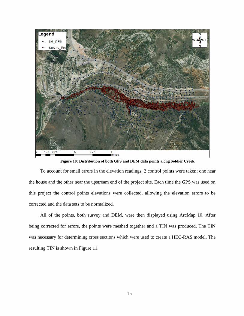
Figure 10: Distribution of both GPS and DEM data points along Soldier Creek.
To account for small errors in the elevation readings, 2 control points were taken; one near
the house and the other near the upstream end of the project site. Each time the GPS was used on
this project the control points elevations were collected, allowing the elevation errors to be
corrected and the data sets to be normalized.
All of the points, both survey and DEM, were then displayed using ArcMap 10. After
being corrected for errors, the points were meshed together and a TIN was produced. The TIN
was necessary for determining cross sections which were used to create a HEC-RAS model. The
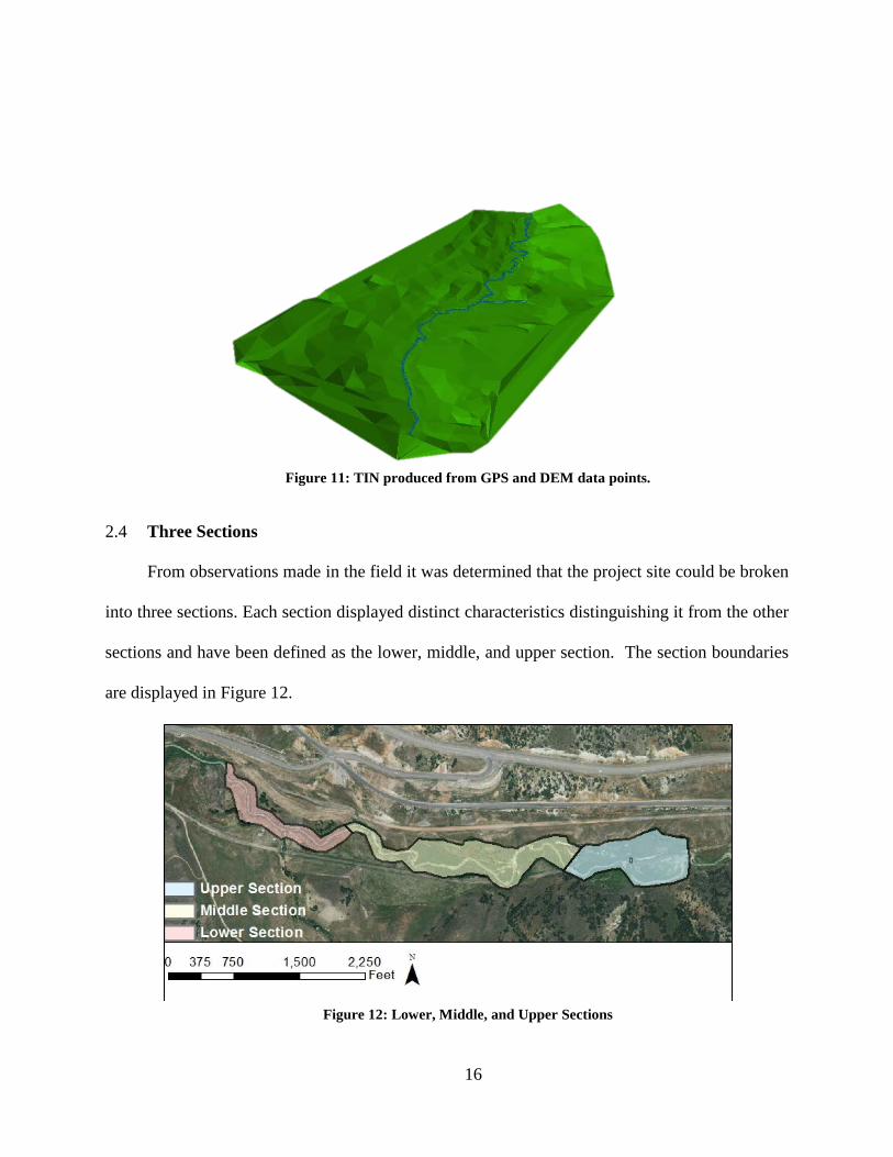
resulting TIN is shown in Figure 11.
16
Figure 11: TIN produced from GPS and DEM data points.
2.4 Three Sections
From observations made in the field it was determined that the project site could be broken
into three sections. Each section displayed distinct characteristics distinguishing it from the other
sections and have been defined as the lower, middle, and upper section. The section boundaries
are displayed in Figure 12.
Figure 12: Lower, Middle, and Upper Sections
17
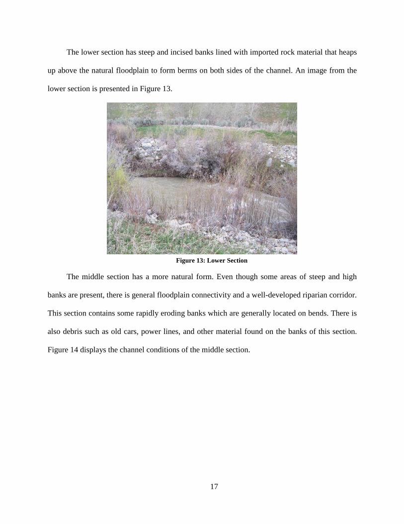
The lower section has steep and incised banks lined with imported rock material that heaps
up above the natural floodplain to form berms on both sides of the channel. An image from the
lower section is presented in Figure 13.
Figure 13: Lower Section
The middle section has a more natural form. Even though some areas of steep and high
banks are present, there is general floodplain connectivity and a well-developed riparian corridor.
This section contains some rapidly eroding banks which are generally located on bends. There is
also debris such as old cars, power lines, and other material found on the banks of this section.
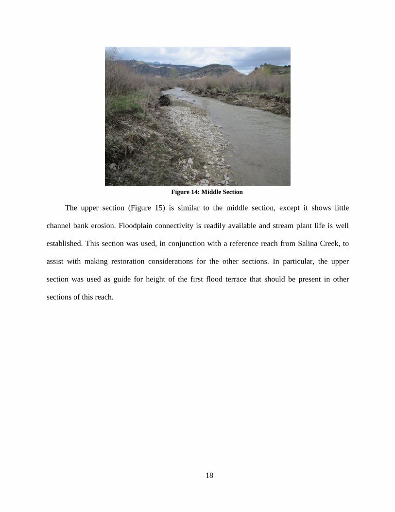
Figure 14 displays the channel conditions of the middle section.
18
Figure 14: Middle Section
The upper section (Figure 15) is similar to the middle section, except it shows little
channel bank erosion. Floodplain connectivity is readily available and stream plant life is well
established. This section was used, in conjunction with a reference reach from Salina Creek, to
assist with making restoration considerations for the other sections. In particular, the upper
section was used as guide for height of the first flood terrace that should be present in other
sections of this reach.

19
Figure 15: Upper Section
2.5 HEC-RAS Model
A HEC-RAS model was built from cross-sections extracted from the TIN shown in Figure
10 above. Cross sections were chosen for reaches of river where the hydrology or
geomorphology of the river changed. The HEC-RAS cross sections for a majority of the project
area are shown in Figure 16.

20
Figure 16: Cross Sections created in HEC-RAS.
A HEC-RAS model is necessary to show which flows will exit the channel and flow onto
the floodplain. In following the Rosgen method (Rosgen D. , 2007), water should flow onto the
floodplain at bankfull flow, which for Soldier Creek, was determined to be about 150 cfs above
the confluence. As mentioned in Table 3, the bankfull flow return interval is approximately 1.75
years.
The HEC-RAS model was run using three different flows. The first flow modeled was the
measured flow on the day that the hydraulic survey was conducted (40.8 cfs). This flow was
chosen to allow for comparison of modeled and observed flow depths and was used for model
calibration. The second flow modeled was the approximate bankfull discharge (180 cfs - below
the confluence). The third flow modeled was the 50 year flood event (1190 cfs).
Cross sections from the Lower, Middle, and Upper Sections are provided in Figures 17,
18, and 19 and show the water surface profiles for the 50-yr flood, bankfull conditions, and the
measured extent.
FullReach
292.1618
244.8914
169.2305
124.1372
66.8826834.97347.931462
L
ak
eFork Upper
3613453.393353.131
3312.9173239.2
3188.4683171.5233089.917
3057.5442937.0142875.87
2708.8522560.2072400.588
2304.58
2283.399
2229.4872138.0482051.6861838.888 Soldie
rCr
eek
Middle
1688.215
LakeForkConf

21
Figure 17: HEC-RAS Lower Section Cross Section Looking Downstream
Figure 18: HEC-RAS Middle Section Cross Section Looking Downstream
200 300 400 500 600 700
5090
5095
5100
5105
SoldierCreek Plan: PreDevPlan 2/28/2013
Station (ft)
Ele
vatio
n (ft
)
Legend
WS 50-yr Flood
WS Bankfull Flow
WS Measured Extent
Ground
Bank Sta
.042
150 200 250 300 350
5122
5124
5126
5128
5130
5132
5134
5136
5138
SoldierCreek Plan: PreDevPlan 2/28/2013
Station (ft)
Ele
vatio
n (ft
)
Legend
WS 50-yr Flood
WS Bankfull Flow
WS Measured Extent
Ground
Bank Sta
.042
22
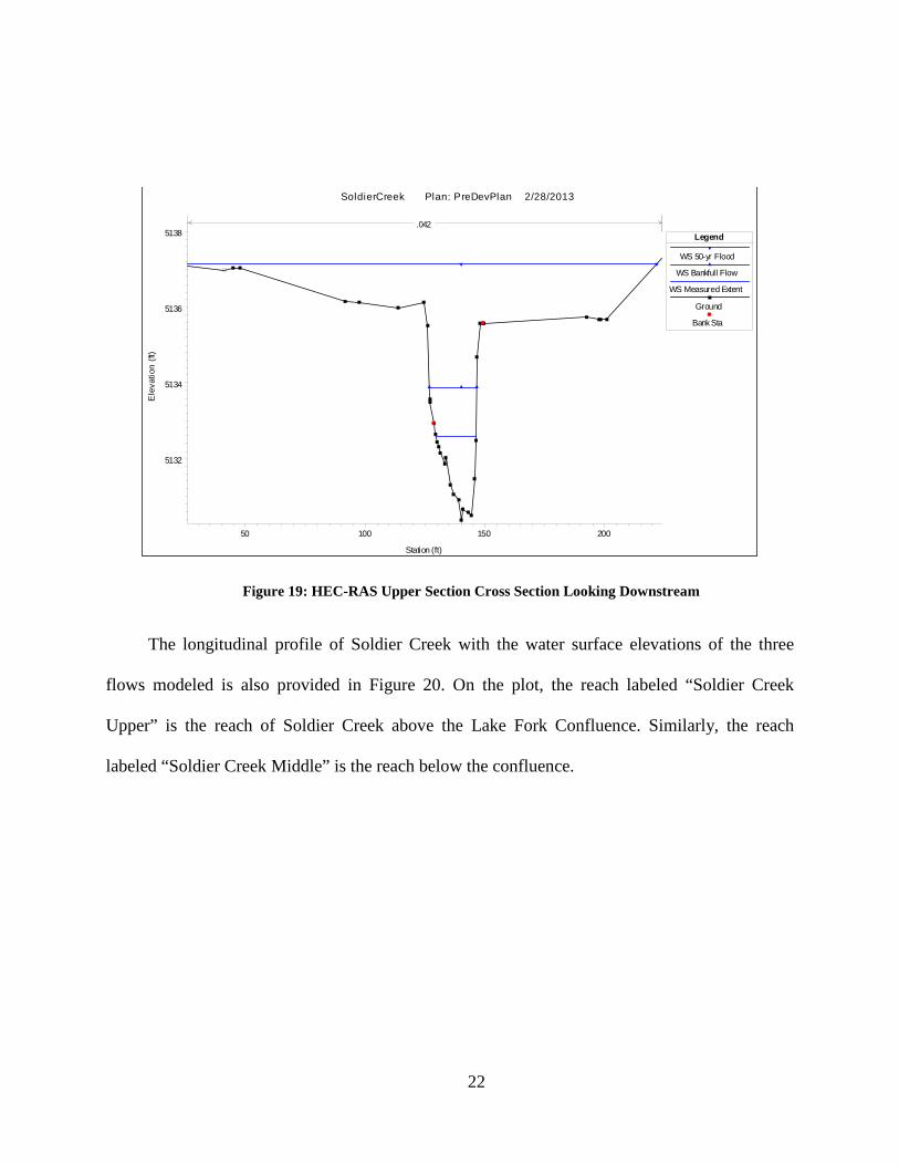
Figure 19: HEC-RAS Upper Section Cross Section Looking Downstream
The longitudinal profile of Soldier Creek with the water surface elevations of the three
flows modeled is also provided in Figure 20. On the plot, the reach labeled “Soldier Creek
Upper” is the reach of Soldier Creek above the Lake Fork Confluence. Similarly, the reach
labeled “Soldier Creek Middle” is the reach below the confluence.
50 100 150 200
5132
5134
5136
5138
SoldierCreek Plan: PreDevPlan 2/28/2013
Station (ft)
Ele
vatio
n (ft
)
Legend
WS 50-yr Flood
WS Bankfull Flow
WS Measured Extent
Ground
Bank Sta
.042

23
Figure 20: Soldier Creek Longitudinal Profile
The results of the HEC-RAS model support the observations made about the three sections
described above. In the middle and upper sections of the property floodplain connectivity is
predicted in the model. The lower section shows no floodplain connectivity even during the 50-
year flood. Furthermore, the longitudinal profile shows a noticeable drop in channel and flow
complexity in the lower section.
2.6 HQI
To further understand Soldier Creek’s potential as a fishery, a fish habitat survey was
performed on the project area. Habitat Quality Index (HQI) (Binns, 1982) was recommended by
UDWR as it is their preferred method. Three sampling locations were chosen; one each for the
lower, middle, and upper sections (Figure 21).
0 2000 4000 6000 8000 10000 120005040
5060
5080
5100
5120
5140
5160
SoldierCreek Plan: PreDevPlan 2/28/2013
Main Channel Distance (ft)
Ele
vatio
n (ft
)Legend
WS 50-yr Flood
WS Bankfull Flow
WS Measured Extent
Ground
SoldierCreek Middle SoldierCreek Upper
24
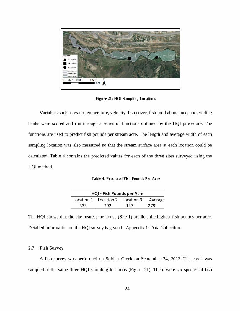
Figure 21: HQI Sampling Locations
Variables such as water temperature, velocity, fish cover, fish food abundance, and eroding
banks were scored and run through a series of functions outlined by the HQI procedure. The
functions are used to predict fish pounds per stream acre. The length and average width of each
sampling location was also measured so that the stream surface area at each location could be
calculated. Table 4 contains the predicted values for each of the three sites surveyed using the
HQI method.
Table 4: Predicted Fish Pounds Per Acre
HQI - Fish Pounds per Acre Location 1 Location 2 Location 3 Average
333 292 147 279 The HQI shows that the site nearest the house (Site 1) predicts the highest fish pounds per acre.
Detailed information on the HQI survey is given in Appendix 1: Data Collection.
2.7 Fish Survey
A fish survey was performed on Soldier Creek on September 24, 2012. The creek was
sampled at the same three HQI sampling locations (Figure 21). There were six species of fish

25
sampled: Brown Trout (BNT), Bonneville Cutthroat Trout (CTT), Mottled Sculpin (MSC),
Leatherside Chub (LSC), Mountain Sucker (MSK), and Long Nosed Dace (LND). The
abundance (count) of each species sampled at all three locations is recorded in Table 5 while the
average weight (W) and length (L) of each species is recoded in Table 6.
Table 5: Fish Species Count
Species Location 1
Location 2 Location 3 Total
BNT 0 3 2 5 CTT 0 1 1 2 MSC 4 80 65 149 LSC 129 62 28 219 MSK 49 176 92 317 LND 51 48 33 132
Table 6: Fish Species Average Weight, and Length
BNT CTT MSC LSC MSK LND W (g) 247.8 44 3.0 10.5 26.0 5.7 L (mm) 292.8 165.5 68.4 95.1 132.1 78.2
Using the stream area the density (fish/surface acre) and biomass (fish/acre) were calculated.
These values are reported in Table 7.
Table 7: Stream Dimensions and Fish Abundance Metrics
Location Length
(ft) Average Width
(ft) Stream Area
(acre) Fish per
Stream Acre Fish Pounds
Per Acre 1 232 16.3 0.087 2686 74.54 2 326 17 0.127 2908 113.26 3 197 15.8 0.072 3091 111.41
These results show a large native fish population in the project reach. The Bonneville
Cutthroat Trout, Mottled Sculpin, Leatherside Chub, Mountain Sucker, and Long Nosed Dace
are all native species to the region. It is noteworthy that there is a significant Leatherside Chub
population in the stream area. The Leatherside Chub is listed as a state sensitive species due to

26
the substantial decrease in its current population (State of Utah Natural Resources - Wildlife
Resources).
The stream reach has a low trout population. Only five Brown Trout and two Bonneville
Cutthroat Trout were sampled. Three Brown Trout and one Cutthroat Trout were sampled at
Location 2. The other two Brown Trout and One Cutthroat Trout were sampled at Location 3.
There were no trout sampled at Location 1. It is unlikely that these fish are native to this stream.
The low numbers and large size of the trout sampled lead to the conclusion that these fish are
transient. It is likely that they were reared in a connecting stream location and have swum to this
location to feed on native minnows. The low trout populations are most likely due to the high
turbidity levels in the stream.
2.8 Reference Reach
Step five of Rosgen’s eight steps for river restoration, entails selecting a reference reach
which can be used to obtain dimensionless ratios for newly designed river reaches. (Rosgen D. ,
2007) Streams were selected as potential reference reaches based on valley type and surrounding
geology. The five streams were Ferron Creek, Salina Creek, White River, Muddy Creek, and Salt
Creek. Using these streams, a regional curve was created that shows the relationship between
bankfull discharge (ft3/s) and drainage area (mi2). This regional curve is found below in Figure
22 with the drainage area plotted on the x-axis and bankfull discharge plotted on the y-axis.

27
Figure 22: Regional Curve (Rosgen D. , 2007)

28
Using the regional curve and with input from local biologists from the Utah Division of
Wildlife Resources (UDWR), Salina Creek was selected as a reference reach. Salina Creek is
located in southern Utah and is relatively undisturbed. A GPS survey, channel measurements,
and sediment samples were collected. The information obtained from measurements taken on
Salina Creek was used as a guideline for appropriate bank slopes above the first terrace. Figure
23 is a picture of Salina Creek and shows its dense riparian vegetation and stable banks. More
detailed information about the reference reach can be found in Appendix 1 Data Collection.
Figure 23: Salina Creek

29
3 RESTORATION DESIGN
3.1 Objectives
• Improve Fish Habitat
• Construct Habitat Ponds for Endangered Spotted Frog
• Build a Dependable Water Diversion
3.2 Improve Fish Habitat
A major component of this project is to improve fish habitat. It has been identified that the
best way to improve habitat is to improve the conditions of the banks along the channel. Key
areas of needed bank improvement have been identified and a plan for improvement at each
location is outlined in this section.
3.2.1 Reconstruction of Banks near the House
The large steep banks on the lower section of the property will need to be reconstructed.
The heaped up banks and imported riprap lining the channel are no longer necessary for flood
prevention because the highway and railroad are no longer in the potential flood prone area.

30
The channel in this section is significantly incised. As previously mentioned, the HEC-
RAS model shows no connectivity to the floodplain even during an extreme flow event. The
historic aerial photography shows that the channel upstream has meandered and adjusted.
However, the reach near the house has remained unchanged, restricted by the channel riprap.
The lower section scored well for habitat quality in the HQI report, but this section
contained 34% less fish pounds per acre then the middle and upper sections. The riprap’s
constriction of natural channel functions is believed to be a contributing factor to the reduced
fish populations. It is assumed that once the geomorphological processes are no longer
constrained by the riprap fish populations will improve.
Figure 24 below displays the banks that will require work in the lower section. This
section is approximately 2000 feet long; it extends from the downstream boundary edge of the
property to roughly 500 feet above the Soldier Creek - Lake Fork Confluence.
Figure 24: Berms to Be Removed
Removal of the berms on both sides of the channel will be necessary in this section to
restore natural channel geomorphology. Figure 25 below displays a profile view of the channel
modification to be performed (cross section location is marked on Figure 24).

31
Figure 25: Excavation Cross Section
Some banks in the section do not have elevated berms as depicted in Figure 25, but are still
heavily incised and lined with riprap and will also be cut back to increase stability and floodplain
connectivity.
There is a distinguishable bankfull depth in this section. Berm removal will not extend into the
bankfull area. All willows removed during reconstruction will be stockpiled during excavation
and replanted along the new channel section just outside of the bankfull area.
A rough estimate of 40,000 cubic yards will be removed from the top of banks in this
reach. All rock material larger than 1.5 will be stockpiled for further stream improvement work
upstream. The remaining material will be piled elsewhere on the property. This location will be
determined by the property owner.
The reference reach can be used as a guide for bank slopes. Outside of the bankfull area
the bank slope should be between 1:5 and 1:10. A sample cross section from Salina Creek
(reference reach) is provided in Figure 26.
5086
5088
5090
5092
5094
5096
5098
5100
5102
5104
5106
0 50 100 150 200 250 300 350
CurrentConditionBermsRemoved
Station (ft)
Elev
atio
n (f
t)

32
Figure 26: Reference Reach Sample Cross Section
3.2.2 Channel Modifications and Considerations
A large amount of sediment in Soldier Creek comes from exposed raw banks within our
reach. A major aspect of this project deals with stabilizing these banks with in-channel
structures. These structures are built with the purpose of redirecting the flow away from the
banks and into the center of the channel. This decreases the shear stresses near the banks, thus
decreasing the amount of erosion. These structures also produce habitat for fish.
A survey of the river led to the identification of 4 key reaches with high rates of erosion.
Different methods and structures were used in each instance to stabilize the banks and channel.
The 4 selected reaches are identified in Figure 27.
Figure 27: Locations of High Erosion Sites
6934
6936
6938
6940
6942
6944
6946
0 20 40 60 80 100 120
Elev
atio
n (ft
)
Station (ft)

33
Location 1
For the first location, high stream velocities have cut into the left bank, leaving a 10 foot
bare wall. The wall is located on a bend after a straight stretch, which increases the power and
velocity of the river as it enters that bend. Figure 28 is a picture looking upstream at the bare wall
with water flowing from the top of the picture to the bottom.
Figure 28: Bare Wall of Location 1 looking upstream.
To stabilize this bank the depression on the left bank will be filled and two J-Hook Vanes
will be installed on the outer bend of the reach. A representation of the location and design of
the J-Hook Vanes is shown below in Figure 29.

34
Figure 29: J-Hook Vanes. Flow is from right to left.
The hole will be filled by layering logs and rocks. The logs will be approximately 1 foot in
diameter and will be approximately 20 feet long. The first layer in the hole will be the logs. They
will be place perpendicular to the flow. To anchor the logs down, rocks will be placed on top of
them to form the second layer. The rocks for the hole can be taken from the stockpile of rocks
taken from the downstream berm removal. The two layers combined should build a bank
approximately 3 to 4 feet high. This will then be covered with top soil and sod taken from the
nearby field.
The J-Hook Vanes will be designed according to instructions given in a report on the
Wildland Hydrology webpage (Rosgen D. , The Cross-Vane, W-Weir and J-Hook Vane
Structures…Their). A description of the design parameters for a J-Hook is found in Figure 30,
taken from the Rosgen article.

35
The structure is designed with the main vane extending away from the outside bank at a
20-30˚ angle and spanning 1/3 of the bankfull width into the channel. From the bankfull height to
the invert rock, the vane is angled downward 2-7% with the rocks being tightly packed together.
The hook extends another 1/3 of the bankfull channel width, but the rocks are placed 3-4 inches
apart. This increases the velocities at this location, deepening the pool that is formed just
downstream of the structure, as well as efficiently passing sediment and debris through the
system.
Figure 30: Design Parameters for J-Hook Vanes (taken from
http://www.wildlandhydrology.com/assets/cross-vane.pdf)
The length of the vane can be determined by using equations given in chapter 11 of the
National Engineering Handbook (NEH) 654 (2007). Both the vane length and vane spacing are

36
functions of the radius of curvature (Rc) of the bend and the bankfull width (W). The departure
angle is the angle between the vane and a line tangent to the bank at bankfull flow. The equations
for vane length and vane spacing are shown in Table 8 and Table 9 respectively.
Table 8: Equations for Calculating Vane Length
Rc/W Departure angle (degrees)
Equation VL=Vane Length (ft)
3 20 VL = 0.0057W + 0.9462 3 30 VL = 0.0089W + 0.5933 5 20 VL = 0.0057W + 1.0462 5 30 VL = 0.0057W + 0.8462
Table 9: Equations for Calculating Vane Spacing
Rc/W Departure angle (degrees)
Equation VS=Vane Spacing (ft)
3 20 VS = -0.006W + 2.4781 3 30 VS = -0.0114W + 1.9077 5 20 VS = -0.0057W + 2.5538 5 30 VS = -0.0089W + 2.2067
By measuring the radius of curvature and bankfull width, the vane length and spacing for
Location 1 could be calculated. The results of these calculations are shown in Table 10.
Table 10: J-Hook Vane Parameters
Parameter Value Bankfull Width (W) 23.3 ft Radius of Curvature (Rc) 40 ft Vane Length 20 ft Vane Spacing 50 ft

37
The minimum rock size can also be calculated using equations given in NEH 654. The
minimum rock size is a function of shear stress in the channel. The shear stress was calculated
using the discharge (Q), the hydraulic radius (R), and the slope (S). There is a considerable
amount of uncertainty in the shear stress values; therefore, a large factor of safety will be used. It
has been determined through familiarity with this type of structure that the minimum rock
diameter should be 1.5 ft. The minimum rock size calculations can be found below in Table 11.
Table 11: Minimum Rock Size Calculation
Parameter Value Flow (Q) 150 cfs Specific Weight 62.4 lb/ft3 Hydraulic Radius (R) 2.17 ft Slope (S) 0.0069 ft/ft Bankfull Shear Stress (τ) 0.93 lb/ft2 Minimum Rock Size Minimum Rock Size * FS
0.25 ft 1.50 ft
To prevent scour that could flank the structure, a cut off sill is installed which extends
from the base of the vane into the bank approximately 5 or 6 feet. These rocks are typically
larger and are placed in a line perpendicular to the stream.
If the bank in which the structure is being installed is higher than the bankfull height of
the river, then a bankfull bench needs to be created. The bench must be cut into the outer bank at
the bankfull height and be approximately 5 feet wide. The bench must also extend a length of 35
feet upstream from the outside bank footer stone and angle back to the stream for a length of
approximately 5 feet downstream. Figure 31 is a cross sectional view of a bankfull bench.
(Rosgen D. , The Cross-Vane, W-Weir and J-Hook Vane Structures…Their)
38
Figure 31: Cross Sectional View of a Bankfull Bench (taken from
http://www.wildlandhydrology.com/assets/cross-vane.pdf).
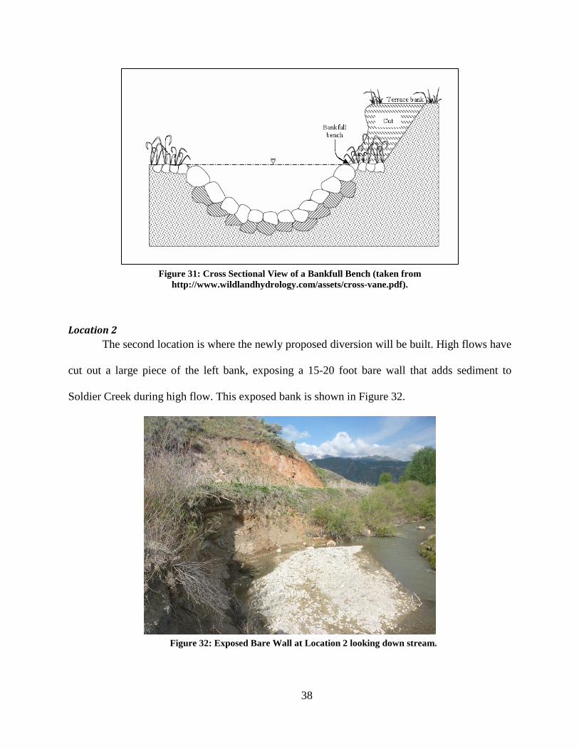
Location 2 The second location is where the newly proposed diversion will be built. High flows have
cut out a large piece of the left bank, exposing a 15-20 foot bare wall that adds sediment to
Soldier Creek during high flow. This exposed bank is shown in Figure 32.
Figure 32: Exposed Bare Wall at Location 2 looking down stream.

39
This location is important not only because of the new diversion structure, but also because
it is the access point to the upstream portion of the property. Without restoration action at this
location, high flows can cut further into this bank, cutting off access to the upper ends of this
property.
To repair this bend, the left bank will be filled into the channel to the edge of the main
flow. Two J-Hook Vanes will be built in addition to the diversion structure as illustrated in
Figure 33. The bank will be extended using the same method used to build the bank on Location
1.
The first J-Hook will be located just upstream from where the erosion begins and the
second will be located approximately 70 feet downstream. The diversion structure will be located
approximately 70 feet downstream from the second structure. The structure design will be
similar to those outlined for Location 1. The Structure Dimensions are provided in Table 12
Table 12: Location 2 Structure Dimensions
Vane length (ft) 20 Vane Spacing (ft) 70 Minimum Rock Size (ft) 1.5

40
Figure 33: Location 2 Design
Location 3 The third location consists of a 20-25 foot exposed wall that is just upstream from the
new diversion structure. The river runs along the base of the wall and is undermining the bank
(Figure 34).

41
Figure 34: Exposed Hill Side at Location 3 looking upstream.
By closer examination, it appears that the channel has migrated to its current location over
the past 30 years, and that a failed beaver dam may have been the trigger that caused the initial
shift. A survey of the area reveals a shallow depression approximately 20-30 feet to the left of
the current river location, which is believed to be the location of the original channel. For this
location it is proposed to re-form this relic channel to receive the flow. The location of the new
channel can be seen in Figure 35.

42
Figure 35: Redesigned Relic Channel at Location 3.
The depression of the relic channel is still present, and will need to be cleared of vegetation
and debris. Using upstream and downstream cross sections the correct relic channel dimensions
can be estimated (Table 13). The dimensions of the relic channel should be checked against the
estimated values. If the relic channel dimensions are not similar to the estimated values, the
channel should be altered to more closely match the estimated dimensions.
Table 13: Estimated Relic Channel Dimensions
Parameter Value Length ~150 ft Bankfull Width ~30 ft Bankfull Depth ~3 ft Slope ~0.008
In order to reestablish the relic channel, the beaver dam remnants will be removed from
the upstream end of the restored relic channel. The existing channel will be plugged at this
location and the channel plug will be constructed like the wood rock fill construction outlined for

43
locations 1 and 2. All willows and sod removed from the relic channel will be saved and used to
plant on top of the plug to further strengthen the bank. The location where the existing channel
and restored channel meet will not be plugged in order to allow for a back water habitat
environment to form.
By returning the river to its previous channel, active erosion of the right bank will cease,
decreasing the sediment load in Soldier Creek.
As noted in Figure 35, it may be necessary to install a J-Hook structure downstream from
the new channel. High velocities exiting the new channel may run directly into the right bank at
the location noted, but it is recommend that construction of such a structure be postponed until
erosion at this location is observed.
Location 4
The final location under consideration for erosion mitigation is the old diversion shown
in Figure 36. Large flows in 2011 dislodged and toppled the rocks from the diversion, re-
directing the flow from the center of the channel into the left bank.
The first step to fix this problem is to remove the remaining rocks from the diversion to
prevent the flow from being directed into the left bank. The next step is to observe the how the
stream reacts when the rocks are removed. If erosion of the left bank continues, then cross vane
rock structures will be used to stabilize this bank. The vane structures will be built with the same
dimensions as the structures described for Location 1. (VS=70 ft, VL=20 ft, Min. rock size=1.5
ft)
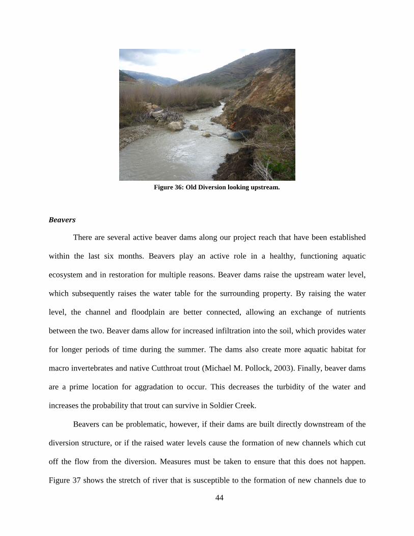
44
Figure 36: Old Diversion looking upstream.
Beavers
There are several active beaver dams along our project reach that have been established
within the last six months. Beavers play an active role in a healthy, functioning aquatic
ecosystem and in restoration for multiple reasons. Beaver dams raise the upstream water level,
which subsequently raises the water table for the surrounding property. By raising the water
level, the channel and floodplain are better connected, allowing an exchange of nutrients
between the two. Beaver dams allow for increased infiltration into the soil, which provides water
for longer periods of time during the summer. The dams also create more aquatic habitat for
macro invertebrates and native Cutthroat trout (Michael M. Pollock, 2003). Finally, beaver dams
are a prime location for aggradation to occur. This decreases the turbidity of the water and
increases the probability that trout can survive in Soldier Creek.
Beavers can be problematic, however, if their dams are built directly downstream of the
diversion structure, or if the raised water levels cause the formation of new channels which cut
off the flow from the diversion. Measures must be taken to ensure that this does not happen.
Figure 37 shows the stretch of river that is susceptible to the formation of new channels due to

45
high water levels. Beaver dams that are compromising the efficiency of the diversion should be
dismantled. The UDWR has many methods for effectively controlling problematic beaver
activity and should be consulted if problems of this nature occur.
Figure 37: Area requiring beaver dam maintenance.
3.2.3 Non-Treated Eroding Banks
There are two eroding banks in the middle section (Figure 38) for which no direct
restoration plan has been made.
Figure 38: Non-Treated Eroding Banks

46
No active restoration was planned for Location 1 (Figure 39) because it is believed that the
degraded banks in this section will improve once the fence outlined in the next section is built.
Also, recent beaver activity has been observed and will help this section to repair itself.
Figure 39: Location 1 Eroding Banks
No restoration was planned for Location 2 (Figure 40) because of beaver activity. A large
beaver dam has recently been built just downstream from this location and water is now backed
up in this area. The near bank stresses have been greatly reduced and the bank is becoming more
stable naturally.
Figure 40: Location 2 Eroding Bank

47
3.2.4 Cattle Grazing/Passive Restoration
Much of the bank instability is caused by the mechanical hoof action by grazing cattle.
Livestock decrease fish habitat and productivity by increasing erosion, sediment, and turbidity.
An example of bank erosion due to cattle grazing can be seen in Figure 39.
To adress this problem, a fence will be built on both sides of the river with styles inserted
in locations dictated by land owner and UDWR personnel (Figure 42). On the south side of the
river the fence will extend from the house upstream to the new diversion to keep livestock out of
the river. This fence will be approximately 3,000 feet long. On the north bank the fence will
extend from the new diversion site down to a quarter mile below the ranch house (approximately
5,000 feet long) (Figure 41).
Fencing will be designed to allow cattle to cross the stream at controlled locations. These
locations will be selected by the land owner. At these gaps the fence will be extended partially
across the stream from both banks to discourage cattle from wandering up or down stream.
Figure 41: Fence Location
The fence will be built to wildlife friendly specifications used by the UDWR. It will
consist of four strands of barbed wire with steel posts spaced 16-1/2 feet apart. The spacing of

48
the barbed wire will be, from the ground up, 16”-8”-8”-10”, with the top wire being no higher
than 42 inches above the ground. There needs to be one wood post for every five metal posts.
The metal posts need to be driven to a minimum depth of 20 inches, while the wood posts need
to be driven 24 inches into the ground (Nielson, 2012). A schematic of the fence is shown in
Figure 42.
Figure 42: Fence Design (Nielson, 2012)
At bends, gates, gullies, and styles H-braces must be installed (Figure 43). Wooden posts
for the H-braces will be placed in line with the fence and set 24 inches into the ground, with the
earth around each post being sufficiently tamped down.

49
Figure 43: H-brace Design (Nielson, 2012)
3.3 Construct Habitat Ponds for Endanger Spotted Frog
Due to habitat degradation along the Wasatch Front, the Columbia Spotted Frog is
included on the Utah Sensitive Species List (State of Utah Natural Resources - Wildlife
Resources). Part of the restoration plan includes building two ponds that will provide breeding
and hibernaculum habitat for this sensitive species. Figure 44 below is a picture of a Columbia
Spotted Frog.

50
Figure 44: Columbia Spotted Frog (State of Utah Natural Resources - Wildlife Resources)
Habitat specifications were provided by Chris Crocket (Crocket, 2012) and (Peterson, 1998).
Frog ponds should have both deep and shallow sections, with the shallow sections being
on the north side of the pond and the deeper sections on the south side. The deeper sections
should have a depth of 1.5-2.0 meters and the shallow sections should be 0.1-0.2 meters deep.
The deeper sections will be used primarily for hiding and hibernating, while the shallower
sections will be used for basking and breeding.
Diverted water needs to flow year round through the deeper section, providing nutrients,
food, and oxygenated water. There should be little or no flow along the shallower northern
shoreline as to not disrupt breeding.
Structures, such as logs, stumps, or root wads, should be randomly placed within the
pond for cover and overwintering habitat. Structures can also be placed within 50 m of the pond
for frogs that overwinter in terrestrial habitats.
There should be little to no canopy cover over the shallow portions. Smaller vegetation
consisting of sedges and rushes can be placed along the shallow edges to provide cover.
Vegetation consisting of cottonwood and willow should exist over the deeper southern side
where breeding does not occur.
51
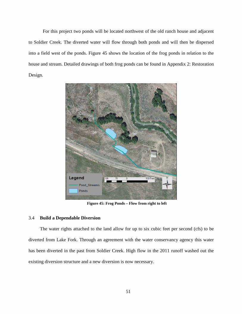
For this project two ponds will be located northwest of the old ranch house and adjacent
to Soldier Creek. The diverted water will flow through both ponds and will then be dispersed
into a field west of the ponds. Figure 45 shows the location of the frog ponds in relation to the
house and stream. Detailed drawings of both frog ponds can be found in Appendix 2: Restoration
Design.
Figure 45: Frog Ponds – Flow from right to left
3.4 Build a Dependable Diversion
The water rights attached to the land allow for up to six cubic feet per second (cfs) to be
diverted from Lake Fork. Through an agreement with the water conservancy agency this water
has been diverted in the past from Soldier Creek. High flow in the 2011 runoff washed out the
existing diversion structure and a new diversion is now necessary.

52
3.4.1 Old Diversion
The washed out diversion structure is depicted in Figure 46. While functioning, it
delivered irrigation water to all of the fields south of the stream on the property (Figure 47).
Figure 46: Old Diversion Structure
Figure 47: Old Diversion Locations and Irrigated Fields – Flow from right to left
The old diversion is located toward the upstream end of the property on a left to right
turning bend. This allowed water to be diverted through the left bank and into the southern fields.
The functioning diversion structure consisted of large rocks piled four to six feet high that
spanned the entire channel width, producing approximately four feet of head.
The canyon wall serves as a hard point and is up against the left side of the diversion. There is no
hard point on the right side of the old diversion.
53
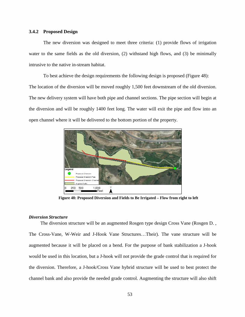
3.4.2 Proposed Design
The new diversion was designed to meet three criteria: (1) provide flows of irrigation
water to the same fields as the old diversion, (2) withstand high flows, and (3) be minimally
intrusive to the native in-stream habitat.
To best achieve the design requirements the following design is proposed (Figure 48):
The location of the diversion will be moved roughly 1,500 feet downstream of the old diversion.
The new delivery system will have both pipe and channel sections. The pipe section will begin at
the diversion and will be roughly 1400 feet long. The water will exit the pipe and flow into an
open channel where it will be delivered to the bottom portion of the property.
Figure 48: Proposed Diversion and Fields to Be Irrigated – Flow from right to left
Diversion Structure The diversion structure will be an augmented Rosgen type design Cross Vane (Rosgen D. ,
The Cross-Vane, W-Weir and J-Hook Vane Structures…Their). The vane structure will be
augmented because it will be placed on a bend. For the purpose of bank stabilization a J-hook
would be used in this location, but a J-hook will not provide the grade control that is required for
the diversion. Therefore, a J-hook/Cross Vane hybrid structure will be used to best protect the
channel bank and also provide the needed grade control. Augmenting the structure will also shift

54
more water toward the head works, ensuring that water will be diverted year around. A
schematic drawing of the diversion to be built is provided in Figure 49.
Figure 49: Schematic Drawing of Diversion Structure (Rosgen D. , The Cross-Vane, W-Weir and J-Hook Vane Structures…Their)
The structure dimensions are as follows:
• Vane length of ~30’.
• Vane Spacing of ~70’
• Minimum Rock Size of ~1.5’
• Average Rock Size of ~3’.
• Angle from bank to stream channel between 2-7%.
55
• Departure Angle between 20 and 25 degrees.
• The hydraulic head produced will be 6 inches (h=6in).
• The footer stones will be buried 2.5 feet (5h).
Because the designed diversion is built into a bank that exceeds bankfull height, a bankfull
bench must be cut into the left bank. The bench must be approximately 5 feet wide and will
extend a length of 35 feet upstream from the left bank footer stone and angle back to the stream
for a length of approximately 5 feet downstream.
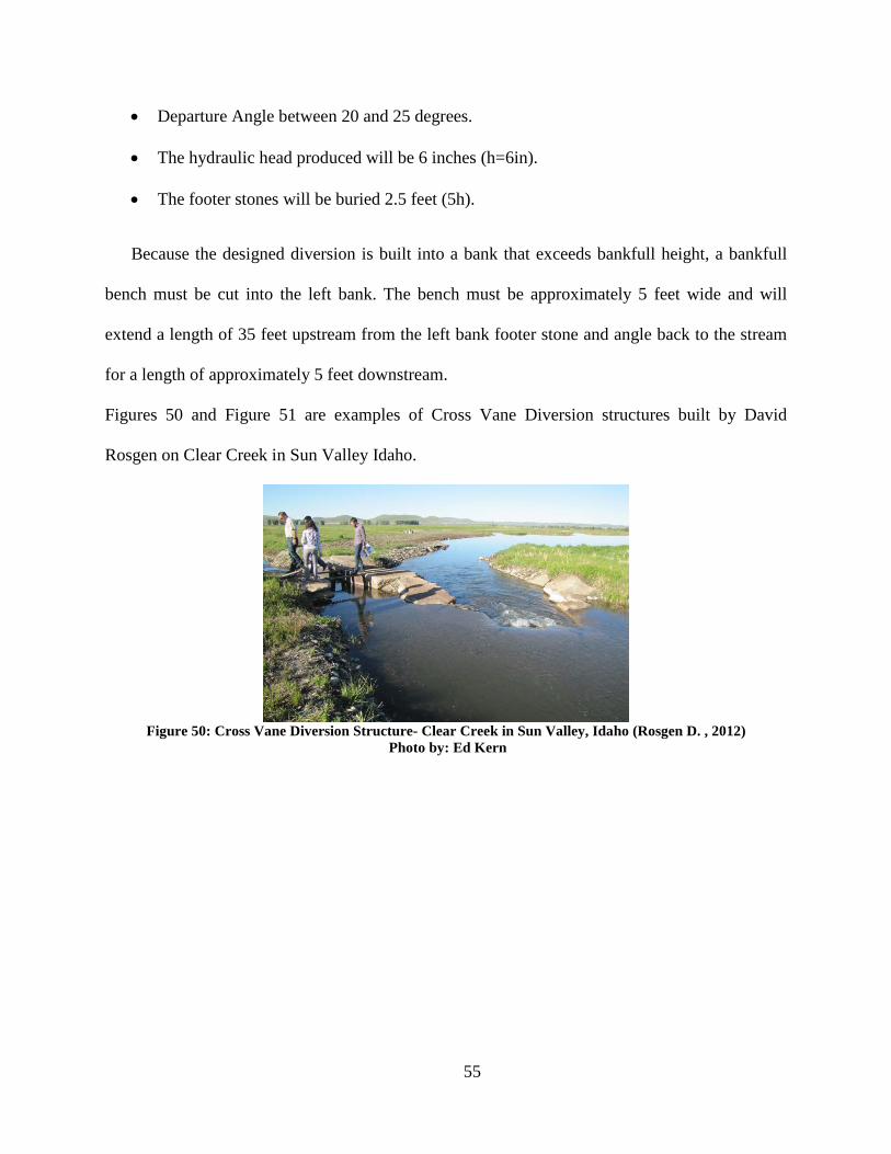
Figures 50 and Figure 51 are examples of Cross Vane Diversion structures built by David
Rosgen on Clear Creek in Sun Valley Idaho.
Figure 50: Cross Vane Diversion Structure- Clear Creek in Sun Valley, Idaho (Rosgen D. , 2012)
Photo by: Ed Kern
56
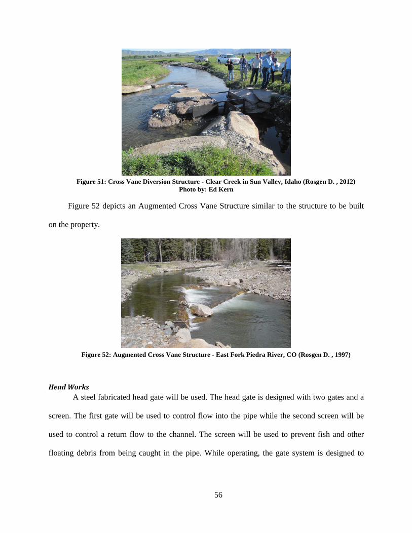
Figure 51: Cross Vane Diversion Structure - Clear Creek in Sun Valley, Idaho (Rosgen D. , 2012)
Photo by: Ed Kern
Figure 52 depicts an Augmented Cross Vane Structure similar to the structure to be built
on the property.
Figure 52: Augmented Cross Vane Structure - East Fork Piedra River, CO (Rosgen D. , 1997)
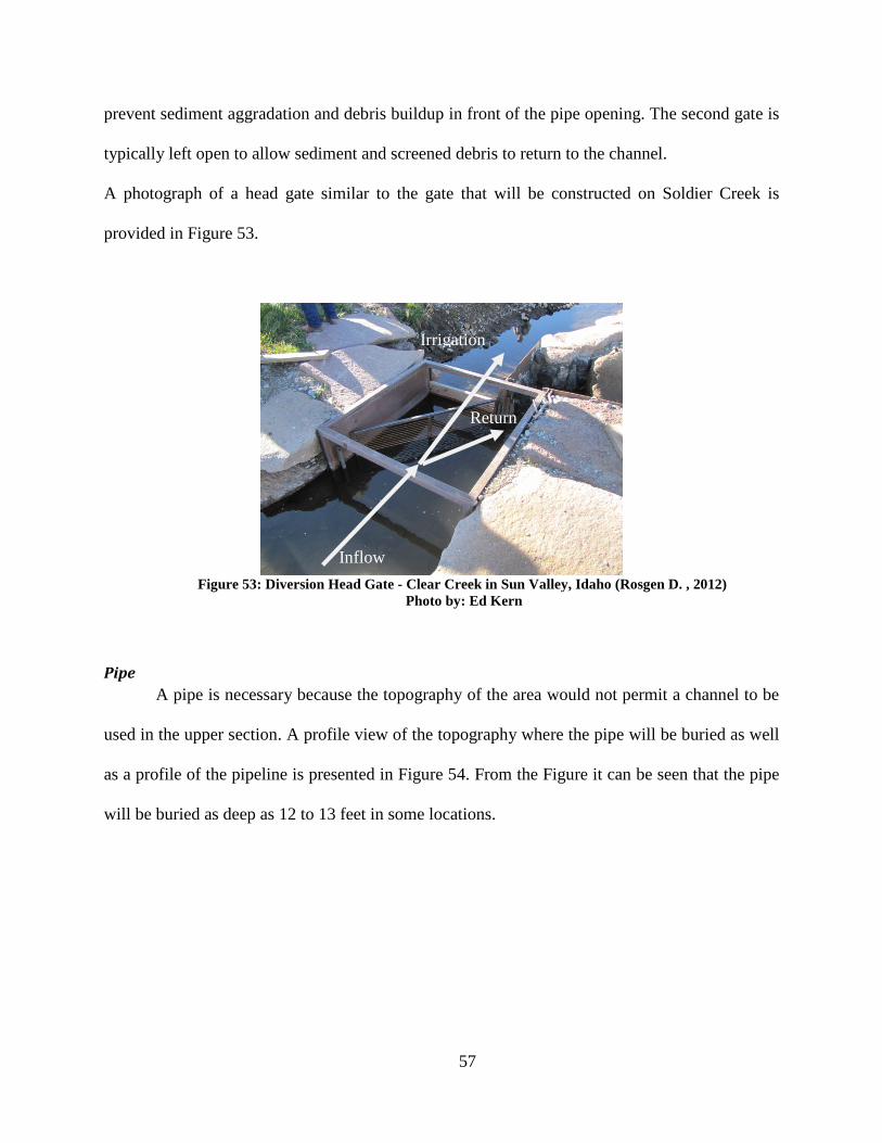
Head Works A steel fabricated head gate will be used. The head gate is designed with two gates and a
screen. The first gate will be used to control flow into the pipe while the second screen will be
used to control a return flow to the channel. The screen will be used to prevent fish and other
floating debris from being caught in the pipe. While operating, the gate system is designed to
57
prevent sediment aggradation and debris buildup in front of the pipe opening. The second gate is
typically left open to allow sediment and screened debris to return to the channel.
A photograph of a head gate similar to the gate that will be constructed on Soldier Creek is
provided in Figure 53.
Figure 53: Diversion Head Gate - Clear Creek in Sun Valley, Idaho (Rosgen D. , 2012)
Photo by: Ed Kern
Pipe A pipe is necessary because the topography of the area would not permit a channel to be
used in the upper section. A profile view of the topography where the pipe will be buried as well
as a profile of the pipeline is presented in Figure 54. From the Figure it can be seen that the pipe
will be buried as deep as 12 to 13 feet in some locations.
Inflow
Irrigation
Return

58
Figure 54: Pipeline Profile
The pipe material will be PVC- PIP (Pipe in Pipe) plastic conduit. It will be 15 inches in
diameter, 1400 feet long, and have the capacity to move 4.5 cfs. Modifications to the pipe length
could be made with more excavation at the outlet.
Pump A pump will be used to provide water to the upper south field (Figure 48). A gas powered
generator will be used to power the pump. The pump and generator will be capable of being
loaded in a truck and carried out to the project site when pumping is needed. The pump will
need to provide 12 ft of hydraulic head and will deliver a flow of 3cfs. In order to achieve this, a
15 Hp pump is required. More pump specifics are provided in Appendix 2: Restoration Design.
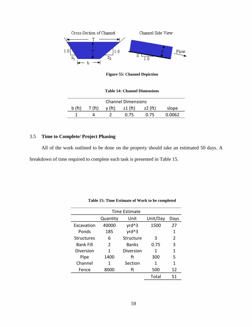
Channel At the end of the pipe a channel will be used to deliver the water to irrigate the fields. A
channel used for the previous diversion already exists. Diverted water will empty into this
channel. The channel will need to be adjusted to fit the dimensions provided in Figure 55 and
Table 14.
51125114511651185120512251245126512851305132
0 200 400 600 800 1000 1200 1400 1600 1800
Elev
atio
n (ft
)
Distance from Diversion (ft)
Pipeline Profile
Land Survey
Pipe Profile
59
Figure 55: Channel Depiction
Table 14: Channel Dimensions
Channel Dimensions b (ft) T (ft) y (ft) z1 (ft) z2 (ft) slope
1 4 2 0.75 0.75 0.0062
3.5 Time to Complete/ Project Phasing
All of the work outlined to be done on the property should take an estimated 50 days. A
breakdown of time required to complete each task is presented in Table 15.
Table 15: Time Estimate of Work to be completed
Time Estimate
Quantity Unit Unit/Day Days
Excavation 40000 yrd^3 1500 27 Ponds 185 yrd^3
1
Structures 6 Structure 3 2 Bank Fill 2 Banks 0.75 3 Diversion 1 Diversion 1 1
Pipe 1400 ft 300 5 Channel 1 Section 1 1
Fence 8000 ft 500 12
Total 51

60
The work to be completed could be phased to be done in a multi-year sequence. A
suggested sequence to complete the project would be: Phase 1 - to reconstruct the banks on the
lower section, Phase 2 – all other tasks.
Table 16: Potential Phase 1: Bank Reconstruction
Phase 1
Quantity Unit Unit/Day Days
Excavation 40000 yrd^3 1500 27
Table 17: Potential Phase 2: Remainder of Project
Phase 2
Quantity Unit Unit/Day Days
Ponds 185 yrd^3
1 Structures 6 Structure 3 2 Bank Fill 2 Banks 0.75 3 Channel 1 Section 1 1
Diversion 1 Diversion 1 1 Pipe 1400 ft 300 5
Fence 6000 ft 500 12
Total 24
The proposed phases are a suggestion and could be altered. While deciding the task
phasing sequence consider: (1) equipment is generally rented on a monthly basis, (2) the rock
and fill materials will be taken from the lower section.
3.6 Cost Estimates
An estimate of the costs required to complete the work presented in this report are
provided in this section. The costs and quantities of materials to be purchased and delivered are
provided in Table 18 and Table 19.

61
Table 18: Stream Improvement Material Costs
Stream Improvements Materials Quantity Units $/unit Delivery Cost
Rock (Structures) 161 Tons $ 25.00 $ 6,650.00 $ 10,675.00 Rock (Fill) 552 Tons $ 25.00 $ 5,250.00 $ 19,050.00
Wood 136 Tons $ 15.00 $ 1,400.00 $ 3,440.00 Fence 8000 ft $ 1.00 $ 500.00 $ 8,500.00
1. Assumes a double load trailer: 38 ton capacity and $350/trip Total $ 41,665.00 2. Estimate by Geneva Rock
This estimate assumes that all materials are purchased and delivered to the project site.
Much of material used will be supplied by the land owner, taken from other locations on the
property. The quantities of materials used and the material cost could be adjusted with the
information provided in Table 19.
Table 19: Diversion Material Costs
Diversion Materials Quantity Units $/unit Delivery Cost
Pipe1 1400 ft $ 8.49 $ 300.00 $ 12,186.00 Pump1 1 - $ 3,500.00 $ - $ 3,500.00
Generator 1 - $ 2,000.00 $ - $ 2,000.00 Diversion Box 1 box $ 500.00 $ - $ 500.00
Diversion Gates 2 gate $ 400.00 $ - $ 800.00 1. Estimate by Howard Irrigation, Springville UT Total $ 17,686.00
The equipment used on this project will need to be rented. For this estimate the cost of
running two track hoes and a dump truck was calculated; and costs presented in Table 20.

62
Table 20: Equipment Rental Costs
Equipment Rental
Equipment Rent Cost Months
Used Fuel
Needed1 Unit $/Unit Fuel Cost Delivery Total Cost
Track Hoe (1)2 $ 6,500.00 2 1950 Gal $ 4.00 $ 7,800.00 $ 700.00 $ 15,000.00
Track Hoe (2)2 $ 6,500.00 2 1950 Gal $ 4.00 $ 7,800.00 $ 700.00 $ 15,000.00
Dump Truck2 $ 11,000.00 2 1950 Gal $ 4.00 $ 7,800.00 $ 700.00 $ 19,500.00 1. Assumed 50 gal/day Total $ 49,500.00
2.Rental from Wheeler CAT, Lindon UT
Labor costs were also considered and are presented in Table 21. This estimate assumes the
use of UDWR crews working at their regular rates.
Table 21: Labor Costs
Wage Pickup Truck
Labor Crew Pay
Periods1 Days Used Wage Cost Rent Cost Miles2 $/mile Cost Cost Total
Heavy Equipment 4 39.00 $ 24,000.00 $ 700.00 1682 $ 0.40 $ 1,372.80 $ 25,373.00
Seasonal 6 55.00 $ 6,000.00 $ 1,050.00 2090 $ 0.40 $ 1,886.00 $ 7,886.00
1. Must pay for full pay period
Total $ 33,259.00
2. 19 miles from Springville Office to Soldier Creek, 200 Miles to get to Springville, 100 miles driven on site
The total costs of the project are summarized in Table 22.
Table 22: Total Costs
Service Cost Materials (Stream) $ 41,665.00
Materials (Diversion) $ 17,686.00 Equipment $ 49,500.00
Labor $ 33,259.00 Total $ 142,110.00

63
4 APPENDIX 1 DATA COLLECTION:
This appendix contains reference materials and more detailed/complete reports of the
data collection presented in Section 2 of this report.
4.1 Hydraulic Survey
A hydraulic Survey was performed for the project site. Notable measurements taken include;
• Slope, Discharge, and Mannings Roughness Coefficient (n)
• Bankfull Measurments
• Sediment Analysis
• Bankfull Discharge
It should be noted that these measurements were taken in localized areas and may not
precisely represent the entire stream reach. It is expected that some variation in reported values
occur throughout the stream reach.
4.1.1 Determining Slope, Discharge, and Manning’s “n”
The measurements and calculations used to determine the roughness are reported below. A
location on the lower end of Soldier Creek near the culvert was chosen. This location was chosen
because it was straight and uniform. Stations were set up at one foot increments across a 13.5

64
foot wide cross section. Note that station 2 and station 14.5 mark the banks. Velocity at each
station was estimated using a Price meter. Each measurement was taken twice at 60% of the
depth. The measurements taken are summarized in Table 23. Velocity is estimated by counting
the number of revolutions in a given amount of time and using the equation in item (i) of the
explanation of Table 23.
Table 23. Velocity Measurements and Calculations
(a) Station (b) Depth taken first time across cross section (c) Number of revolutions first time across cross section (d) Depth taken second time across cross section (e) Number of revolutions second time across cross section (f) Time period in which revolutions were counted (both times across) (g) Average of (b) and (d) (h) Average of (c) and (e)
(i) 𝑉𝑒𝑙𝑜𝑐𝑖𝑡𝑦 (𝑓𝑝𝑠) = 2.2048 ∗ 𝑅𝑒𝑣𝑜𝑙𝑢𝑡𝑖𝑜𝑛𝑠 (𝑟𝑒𝑣./𝑠) + 0.0178
Slope was measured using a surveying level and level rod. The elevation and depth of two
riffles were used, one upstream and the other downstream of the level. The distance from the
(a) Station
(ft)
(b) Depth 1
(ft)
(c) Revolutions 1
(d) Depth 2
(ft)
(e) Revolutions 2
(f) Time (sec)
(g) Average Depth
(ft)
(h) Average
Revolutions
(i) Velocity
(fps)
14.5 0 - 0 - - 0 - - 13 1.1 26 1.1 28 60 1.10 27 1.0 12 1.3 42 1.3 37 60 1.30 39.5 1.5 11 1.45 61 1.4 59 60 1.43 60 2.2 10 1.6 59 1.5 62 60 1.55 60.5 2.2
9 1.55 64 1.5 65 60 1.53 64.5 2.4 8 1.55 65 1.5 67 60 1.53 66 2.4 7 1.65 70 1.55 78 60 1.60 74 2.7 6 1.7 83 1.6 85 60 1.65 84 3.1 5 1.9 65 1.6 73 60 1.75 69 2.6 4 1.9 59 1.8 57 60 1.85 58 2.1 3 1.8 62 1.75 58 60 1.78 60 2.2 2 1.55 40 1.55 45 60 1.55 42.5 1.6
1 0 - 0 - - 0 - -
Overall Average Depth: 1.55
Mean Velocity: 2.2

65
level to each point was estimated using 100 times the distance between the stadia marks. A
summary of the measurements recorded are shown in Table 24.
Table 24. Slope Measurements
The slope of the water surface was found in the following manner. The run was calculated
as the sum of the distances to each point from the level rod. The rise was found as the difference
between the downstream elevation minus the downstream depth and the upstream elevation
minus the upstream depth. The slope of the water surface was found by dividing the rise by the
run. A summary of these calculations is displayed in Table 25.
Table 25. Slope Calculations
Run = Distance(DS) + Distance(US) Rise = [Elevation(DS)-Depth(DS)] –[Elevation (US)-Depth(DS)] Slope = Rise/Run
The cross sectional area and discharge in the channel were calculated by dividing the cross
section into smaller areas. The boundaries of each area straddle a station and velocity
measurement. In this way, an area and discharge for each station was found. The area of each
division was found using the area of a trapezoid formula. The total cross sectional area and the
Dow
nstr
eam
Elevation 5.82 - ft
Depth 1.4 - ft
Stadia 4.84 6.80 ft
Distance 196 - ft
Ups
trea
m Elevation 3.95 - ft
Depth 0.9 - ft
Stadia 2.85 5.05 ft
Distance 220 - ft
Run 416 ft Rise 1.37 ft
Slope (S) 0.003293 ft/ft

66
total discharge was found by summing the respective divisions. Table 26 contains a summary of
the calculations performed and Figure 56 shows a plot of the cross section and the area divisions.
Table 26. Area and Discharge Calculations
(a) Station at the center of the area (b) Depth on right side of the area (c) Depth on the left side of the area (d) Top width of the area (e) 𝐴𝑟𝑒𝑎 (𝑓𝑡2) = 1
2∗ �(𝑏) + (𝑐)� ∗ (𝑑)
(f) Velocity from Table 1, Column (i) (g) 𝐷𝑖𝑠𝑐ℎ𝑎𝑟𝑔𝑒 (𝑐𝑓𝑠) = 𝑉𝑒𝑙𝑜𝑐𝑖𝑡𝑦 (𝑓𝑝𝑠) ∗ 𝐴𝑟𝑒𝑎 (𝑓𝑡2)
(a) Station
(b) Depth1
(ft)
(c) Depth2
(ft)
(d) Base (ft)
(e) Area (ft2)
(f) Velocity
(fps)
(g) Discharge
(cfs) 13 0 1.20 2 1.20 1.0 1.2 12 1.20 1.36 1 1.28 1.5 1.9 11 1.36 1.49 1 1.43 2.2 3.2 10 1.49 1.54 1 1.51 2.2 3.4
9 1.54 1.53 1 1.53 2.4 3.7 8 1.53 1.56 1 1.54 2.4 3.8 7 1.56 1.63 1 1.59 2.7 4.4 6 1.63 1.70 1 1.66 3.1 5.2 5 1.70 1.80 1 1.75 2.6 4.5 4 1.80 1.81 1 1.81 2.1 3.9 3 1.81 1.66 1 1.74 2.2 3.9 2 1.66 0 1.5 1.25 1.6 2.0
Cross Sectional Area: 18.3 Total Discharge: 40.8

67
Figure 56, Cross section with area calculation divisions
Table 26 shows the calculations for the wetted perimeter. The wetted perimeter is
calculated as the sum of the distances between each station. The distance was calculated using
the distance formula.
0
1
2
0 1 2 3 4 5 6 7 8 9 10 11 12 13 14 15 16De
pth
(ft)
Station (ft)
Cross SectionArea Divisions
0
1
2
0 1 2 3 4 5 6 7 8 9 10 11 12 13 14 15 16
Dept
h (ft
)
Station (ft)
Cross SectionArea Divisions

68
Table 27. Wetted Perimeter Calculations
(a) Stations (b) Depth to point on right (c) Depth to point on left (d) Difference between depths (e) Horizontal width between points (f) 𝐿𝑒𝑛𝑔𝑡ℎ(𝑓𝑡) = �(𝑑)2 + (𝑒)2
Manning’s roughness coefficient was calculated using the parameters calculated above
and Manning’s equation (see Equation 1). It was also calculated using Rosgen’s method found in
the National Engineering Handbook section 654 in Figure 11-7 (see Equation 2). The results of
these calculations are summarized in Table 28. Bottom shear stress was also calculated using
Equation 3 for the channel and the results are shown in Table 29.
(a) Station
(b) Depth1
(ft)
(c) Depth2
(ft)
(d) Rise (ft)
(e) Run (ft)
(f) Length
(ft) 1-2 1.55 0.00 1.55 1.00 1.84 2-3 1.78 1.55 0.23 1.00 1.03 3-4 1.85 1.78 0.07 1.00 1.00 4-5 1.75 1.85 0.10 1.00 1.00 5-6 1.65 1.75 0.10 1.00 1.00 6-7 1.60 1.65 0.05 1.00 1.00 7-8 1.53 1.60 0.07 1.00 1.00 8-9 1.53 1.53 0.00 1.00 1.00 9-10 1.55 1.53 0.02 1.00 1.00 10-11 1.43 1.55 0.12 1.00 1.01 11-12 1.30 1.43 0.13 1.00 1.01 12-13 1.10 1.30 0.20 1.00 1.02 13-14.5 0.00 1.10 1.10 1.50 1.86
Wetted Perimeter: 14.7
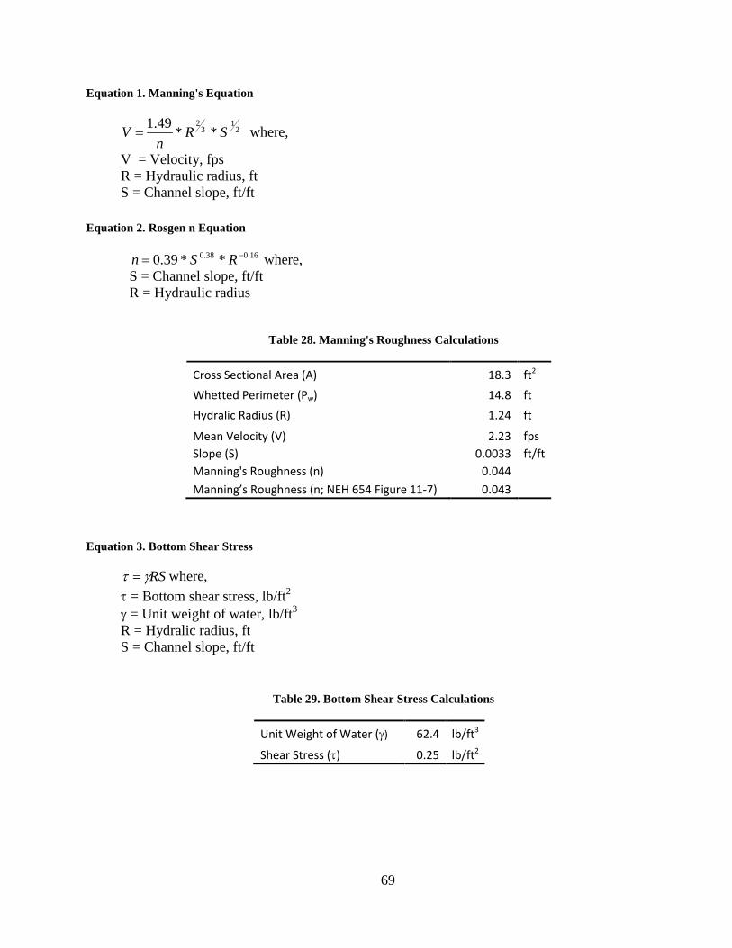
69
Equation 1. Manning's Equation
21
32
**49.1 SRn
V = where,
V = Velocity, fps R = Hydraulic radius, ft S = Channel slope, ft/ft
Equation 2. Rosgen n Equation
16.038.0 **39.0 −= RSn where, S = Channel slope, ft/ft R = Hydraulic radius
Table 28. Manning's Roughness Calculations
Equation 3. Bottom Shear Stress
RSγτ = where, τ = Bottom shear stress, lb/ft2
γ = Unit weight of water, lb/ft3 R = Hydralic radius, ft S = Channel slope, ft/ft
Table 29. Bottom Shear Stress Calculations
Cross Sectional Area (A) 18.3 ft2 Whetted Perimeter (Pw) 14.8 ft Hydralic Radius (R) 1.24 ft
Mean Velocity (V) 2.23 fps Slope (S) 0.0033 ft/ft Manning's Roughness (n) 0.044
Manning’s Roughness (n; NEH 654 Figure 11-7) 0.043
Unit Weight of Water (γ) 62.4 lb/ft3
Shear Stress (τ) 0.25 lb/ft2

70
4.1.2 Sediment Analysis
A Wolman Pebble Count analysis was performed on a stretch of river near the locations
that the bankfull measurements were taken. For each pebble count analysis one hundred samples
were randomly selected and measured. The procedure used to achieve random selection was as
follows:
Start at one bank and work diagonally across the cross section stepping heal to toe.
After every step select a sample from the stream substrate that lies at the point of the toe.
Do not look at the substrate, rather blindly reach to the bottom and select the first piece of
substrate that your finger touches.
Measure the sample using the gravelometer. Record the smallest size that the sample will pass
through.
The data recorded was then analyzed using a particle size distribution method. The D16,
D50, and D84 were all interpolated off of the particle size distribution charts provided in Figure
57 and are reported in Table 30.
Figure 57: Wolman Pebble Count Particle Size Distribution
0
10
20
30
40
50
60
70
80
90
100
1101001000
Perc
ent F
iner
(%)
Diameter( mm)
Site 2
Site 1

71
Table 30: Wolman Pebble Count
Wolman Pebble Count
Percentile Diameter (mm) Site 1 Site 2
D16 8 <2 D50 17 47 D84 46 102
Surficial sediment samples were also analyzed. A total of 4 samples were taken. The
location of each sample is displayed in Figure 58. These samples were collected by inserting a
bottomless 50 gallon drum into the stream substrate. Water was then extracted from the drum to
allow access to the substrate material. Bed armor and subsurface material was taken from each
applicable location (no apparent bed armor at location 3). These samples were taken to the lab to
be dried and sieved. The sieved samples were weighed and a particle size distribution analysis
was performed (Figure 59). The D16, D50, and D84 were all extrapolated using the particle size
distribution graph (Table 31).
Figure 58: Surficial Sediment Sample Locations
Location 2 Location 3
Location
Location

72
Figure 59: Surficial Sediment Sample, Particle Size Distribution
Table 31: Surficial Sediment Sample, Table of Percentiles
Percentile Location 1 Location 2 Location 3 Location 4 Armor Bed Armor Bed N/A Armor Bed (mm) (mm) (mm) (mm) (mm) (mm) (mm)
D16 12 0.6 18 2.2 0.5 42 1.5 D50 102 9 50 13 16 90 15 D84 137 45 92 38 65 135 40
4.1.3 Bankfull Indices
Visual inspection of the Soldier Creek project site was performed in order to determine
certain indicators used in the identification of the bankfull stage dimensions. Bankfull refers to
the elevation of the water surface where flooding begins (the water level exceeds the channel
banks and enters the floodplain). The flow at this level has been labeled as the effective
discharge. This discharge has been identified as the stream discharge that is able to transport the
most sediment over a given time span. Therefore; the effective discharge value is most readily
0.00%
10.00%
20.00%
30.00%
40.00%
50.00%
60.00%
70.00%
80.00%
90.00%
100.00%
0.1110100Size [mm]
Location 1,ArmorLocation 1, Bed
Location 2,ArmorLocation 2, Bed
Location 3
Location 4,ArmorLocation 4, Bed

73
used in stream restoration design as it has been shown to have the greatest influence on the
channel formation, and maintenance over time. Table 32 identifies the field indicators that were
assessed in performing this analysis. While subjective in nature these indices help to provide a
starting point for the bankfull stage assessment.
Table 32: Bankfull Indices Indicators (NEH 654)
Two areas were measured for bankfull dimensions. Figure 60 depicts the areas chosen.
These areas appeared to be in a relatively stable condition with easily identifiable bankfull
indicators. Each measurement was also taken in a riffle section.

74
Figure 60: Bankfull Identification Sites
Areas where indicators were identified were marked and assessed along a section
measuring approximately 200 feet in length. These indicators were assessed as a whole and an
approximation of the bankfull level along the right bank was determined. Once this level was
determined a string line was placed across the stream in order to determine the level on the left
bank. A measurement was taken from the string line to the THALWEG. This was determined to
be the bankfull depth measurement. By multiplying the bankfull depth measurement by a factor
of 2 the flood prone depth measurement was found. An additional string line was placed at this
elevation across the stream and the width measured. Using these string lines the bankfull width
and the flood prone width were determined. These values were used to determine the
entrenchment ratio of the stream. Equation 4 details the calculation of the entrenchment ratio.
Equation 4: Entrenchment Ratio
Entrenchment Ratio ER = Flood Prone Width/Bankfull Width Figure 61 depicts the string line that has been placed over the creek at site 1 to identify the flood
prone level measurement.

75
Figure 61: Determination of Bankfull Indices
Table 33 identifies the values determined in performing the bankfull analysis.
Table 33: Bankfull Indices Values
Site Bankfull Depth Bankfull Width, Flood Prone Entrenchment Measurement, ft ft Width, ft Ratio 1 1.75 20 26.75 1.34 2 1.75 18.4 25.5 1.39

76
4.1.4 Stream Profiles
1541
1542
1543
1544
1545
1546
1547
1548
1549
1550
1551
0.0 200.0 400.0 600.0 800.0 1000.0 1200.0 1400.0
Elev
atio
n (m
)
Station (m)
Culver to West Boundary of Property
1549
1550
1551
1552
1553
1554
1555
1556
1300.0 1400.0 1500.0 1600.0 1700.0 1800.0 1900.0 2000.0 2100.0
Elev
atio
n (m
)
Station (m)
Lower Section

77
1554
1555
1556
1557
1558
1559
1560
1561
1562
1563
1564
1900.0 2100.0 2300.0 2500.0 2700.0 2900.0 3100.0 3300.0
Elev
atio
n (m
)
Station (m)
Middle Section
1563
1564
1564
1565
1565
1566
1566
1567
1567
3100.0 3150.0 3200.0 3250.0 3300.0 3350.0 3400.0
Elev
atio
n (m
)
Station (m)
Top Section

78

79
4.1.5 Stream Stats
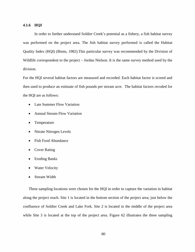
80
4.1.6 HQI
In order to further understand Soldier Creek’s potential as a fishery, a fish habitat survey
was performed on the project area. The fish habitat survey performed is called the Habitat
Quality Index (HQI) (Binns, 1982).This particular survey was recommended by the Division of
Wildlife correspondent to the project – Jordan Nielson. It is the same survey method used by the
division.
For the HQI several habitat factors are measured and recorded. Each habitat factor is scored and
then used to produce an estimate of fish pounds per stream acre. The habitat factors recoded for
the HQI are as follows:
• Late Summer Flow Variation
• Annual Stream Flow Variation
• Temperature
• Nitrate Nitrogen Levels
• Fish Food Abundance
• Cover Rating
• Eroding Banks
• Water Velocity
• Stream Width
Three sampling locations were chosen for the HQI in order to capture the variation in habitat
along the project reach. Site 1 is located in the bottom section of the project area; just below the
confluence of Soldier Creek and Lake Fork. Site 2 is located in the middle of the project area
while Site 3 is located at the top of the project area. Figure 62 illustrates the three sampling

81
locations. The measurements were all taken on the same day in late-August from 9 AM to 12
PM.
Figure 62: HQI Sampling Locations
Water Quality Water quality measurements were collected at each of the three locations (Table 34).
Each sample was collected in a riffle zone at the top of the stream reach. The first site sampled
was Site 1, then Site 2, and finally Site 3. The sampling occurred during a 3 to 4 hour period, this
could have attributed to a slight ambiguity in the temperature reading caused by raising
temperatures from the morning to afternoon hours.
Only the NO3- and temperature readings are considered in the HQI report. Both were given high
rankings according to the HQI method. However, inadequate temperature measurements were
taken. To accurately score the temperature rating of the stream a temperature study would need
to be conducted. The study would include measurements taken throughout the year and at varied
times of the day.
The pH, ammonia (NH4+), Total Dissolved Solids (TDS), Turbidity, and Dissolved Oxygen
(DO) were also measured.

82
Table 34: Water Quality Measurements
Location Temp pH NO3- NH4+ TDS Turbidity LDO LDO °F mg/l mg/l g/l NTU % Sat mg/l
1 60.30 8.27 0.18 1.70 0.40 46.94 106.19 8.73 2 65.45 8.54 0.22 1.55 0.40 41.06 109.20 8.50 3 66.77 8.52 0.22 1.53 0.40 47.83 105.18 8.06 Average 64.17 8.44 0.21 1.59 0.40 45.28 106.86 8.43
Benthic Macroinvertebrates A Benthic Macroinvertebrate sample was collected at each of the three HQI sampling
locations. The Benthic Macroinvertebrates are used to provide a fish food abundance estimate.
Samples were collected using a Surber Sampler. The sample was collected in a riffle at the top of
each sample location. While collecting the sample, the surber sampler was first placed flat on the
channel bottom. Then all of the rocks that lied within the frame were scrubbed clean to a depth
of approximately 6 inches.
The invertebrates were then counted and roughly identified on site (Table 35). The
invertebrates were identified as Stonefly (Plecoptera), Mayfly (Ephemeroptera), Caddisfly
(Trichoptera), or other. For Site 1 the sample was counted until a quantity of 500 was achieved.
This was done because the threshold for the highest rating in the HQI is 500.
Table 35: Count of Benthic Macroinvertebrates
Location Stonefly (Plecoptera)
Mayfly (Ephemeroptera)
Caddisfly (Trichoptera) Other Total
Site 1 114 0 356 30 500 Site 2 96 1 409 45 551 Site 3 39 4 198 78 319
Cover, Width, and Eroding Banks The cover, width, and eroding banks were measured for each site. The measurements
were taken using standard field measuring tape.

83
Cover was defined as anything in the stream that might serve as a resting, hiding, or sheltering
location for fish (Table 36).
Table 36: Cover, Width, and Eroding Banks
Location Cover Width Eroding Banks
% ft % Site 1 27.5% 22.25 5% Site 2 20.0% 20.4 8% Site 3 8.8% 18.75 10%
Late Summer and Annual Flow There is no gauge station on Soldier Creek so in order to assess the Late Summer Flow
and Annual Flow Variability the flow patterns of the three gauged streams used for the regional
curve were analyzed. The gauge information came from the U.S. Geological Survey website.
The Late Summer Flow Index was calculated using the average daily flow values. The average
daily flows from August 1st to September 15th were averaged (CPF) and then divided by the
annual average daily flow (ADF). The Annual Flow Variability was calculated by dividing the
maximum average monthly flow by the minimum average monthly flow. The results of the
analysis are presented in Table 37.
Table 37: Late Summer and Annual Flow
Stream CPF/ADF ASFV Salina Creek 0.75 10.33 Ferron Creek 0.54 31.54 White River 0.22 38.46
Summary All of the variables were scored and ran through a series of functions outline by the HQI
procedure. The functions are used to predicted fish pounds per stream acre. Table 38 contains the
predicted values for each of the three sites surveyed using the HQI method.

84
Table 38: Predicted Fish Pounds Per Acre
HQI - Fish Pounds per Acre Site 1 Site 2 Site 3 Average 333 292 147 279
4.2 Salina Creek
Salina Creek: Stream Survey Jared Erickson; Jeremy Payne October 5, 2012
Figure 63: Longitudinal Profile for Salina Creek
94
96
98
100
102
104
0 100 200 300 400 500 600
Rela
tive
Ele
vaio
n [f
t]
Distance From the Most Upstream Point [ft]
Salina Creek - Longitudinal Profile Channel BottomWater SurfaceBankfull
94
96
98
100
102
104
0 100 200 300 400 500 600
Rela
tive
Ele
vaio
n [f
t]
Distance From the Most Upstream Point [ft]
Salina Creek - Longitudinal Profile Channel BottomWater SurfaceBankfull

85
Table 39: Comparison Chart Between Salina Creek and Soldier Creek
Comparison Between Salina Creek And Soldier Creek Property (Bankfull) Salina Creek Soldier Creek Q (cfs) ~100 170 Return Period (yr) ~1.5 1.5 A (ft2) 20 24.44 WP (ft) 19 19.71 R (ft) 1.053 1.24 S (ft/ft) 0.00958 0.003/0.0055/0.01 Manning’s “n” 0.0335 0.044 Rosgen Calssification B3c (C3) F3/B4c/F4 D16 (mm) 65 42 D50 (mm) 120 90 D84 (mm) 210 135 Entrenchment Ratio 1.95 <1.4/1.42/1.38 W/D Ratio 11.35 10.71/13.48 Sinuosity 1.48/1.09 1.18/1.35/1.36 Drainage Area (mi) 52 236
The bankfull Q and return for Salina Creek are only approximates because many different
methods were employed (Regional Curve, Manning’s “n”, Log Pearson) to determine these
values and the values varied between methods.
For Solder Creek, many of the columns contain 3 values; this corresponds to the 3
different locations where samples were collected. The 3 different collection sites are shown in
the map below. Sediment samples were collected from the pavement layer in a riffle zone. There
is more information on the sediment collection later on in the report.
Site 1 Site 2 Site 3

86
Table 40: Channel Dimension Ratios
Channel Dimensions mean riffle depth 1.4 ft riffle area 23.71 ft2 mean pool depth 2.85 ft pool area 50.94 ft2 mean pool depth/ mean riffle depth 2.04
pool area/ riffle area 2.15
max riffle depth 2.26 ft max riffle depth/ mean riffle depth 1.61 max pool depth/ mean riffle depth 3.49
point bar slope
Riffle Width 17.67 ft Streamflow: Estimated Bankfull Velocity 4.5 ft/s Pool width 17.86 ft Streamflow: Estimated Bankfull Discharge 90 ft3/s Pool width/ riffle width 1.01
Estimating Method manning
max pool depth 4.89 ft Drainage Area 58.1 mi2
Table 41: Channel Pattern Ratios
Channel Pattern
mean min max
mean min max
Meander length 286 190 375 ft Meander length ratio 16.18 10.75 21.22 radius of curvature 64.4 35.9 113.5 ft radius of curvature/riffle width 3.64 2.03 6.42 belt width 62.3 42.7 98 ft meander width ratio 3.54 2.41 5.55 individual pool length 14.75 13 16 ft pool length/riffle width 0.83 0.74 0.91 pool to pool spacing 135.3 97 202 ft pool to pool spacing/ riffle width 7.66 5.49 11.43

87
Table 42: Channel Profile Ratios
Channel Profile
Valley Slope 0.0144 ft/ft Average water surface slope 0.00883 ft Sinuosity 1.48
Stream length 277.4 ft valley length 254.4 ft Sinuosity 1.09
low bank height start 2.78 ft max riffle depth start 2.26 ft bank height ratio LBH/maxriffledepth
start 1.23
end
ft end 1.85 ft end
Facet Slopes mean min max Dimmensionless geometry ratios mean min max
Riffle slope 0.01 0.006 0.02 Riffle slope/average water surface slope 1.13 0.68 1.92
run slope 0.07 0.045 0.11 run slope/average water surface slope 7.93 5.09 12.23
pool slope 0.008 0 0.02 pool slope/average water surface slope 0.91 0.00 1.92
glide slope -0.056 -0.048 -0.1 glide slope/average water surface slope -6.34 -5.43 -7.13
Feature Midpoint mean min max
riffle depth 1.4 0.46 2.26 riffle depth/mean riffle depth 1 0.329 1.61
run depth 1.97 0.68 2.8 run depth/mean riffle depth 1.4 0.49 2
pool depth 2.85 1.18 4.89 pool depth/mean riffle depth 2.04 0.84 3.49
glide depth 1.94 0.78 3.39 glide depth/mean riffle depth 1.39 0.56 2.42
Tables 39 - 41 contain many of the dimensionless ratios that will be needed to design the
new channel at Soldier Creek. These ratios are most important because on Soldier Creek we are
not considering a priority 1 restoration; rather we plan on selecting specific hotspot locations
where erosion and bank stabilization are a problem. These ratios will help us determine how to
restore and stabilize the channel without severely changing the profile of the river (riffle, run,
pool, glide).
Channel Materials
Sediment samples were collected and analyzed. There were two separate sets of
sediment material collected. The first set is the armor layer and sub armor layer collected from a
riffle zone. The second is the armor and sub armor layer collected from a point bar. The D16,
D35, D50, D84, D95, and D100 for all four are recorded, as well as the combined particle size
percentiles in Table 43.

88
Table 43: Sediment Sample Salina Creek
Channel Materials
Pavement (mm)
Subpavement (mm)
PB Subpavement (mm)
PB Pavement (mm)
Combined (mm)
D16 65 21 2.2 5.1 3 D35 100 29 9 11 19 D50 120 35 10.6 20 48 D84 210 125 68 130 130 D95 245 190 100 155 210 D100 250 250 127 200 250
These percentiles were read off of the graph provided in figure 66. This graph displays
the five mentioned particle size distributions. The particle size in millimeters is graphed on the
x-axis with the percent finer graphed on the y-axis.

89
0%
10%
20%
30%
40%
50%
60%
70%
80%
90%
100%
0.10 1.00 10.00 100.00 1000.00
% P
assi
ng
Size [mm]
Subpavement
Pavement
Point Bar Subpavement
Point Bar Pavement
Combined

90
Figure 64: Particle Size Distribution for Salina Creek
The channel measurements taken include 12 bankfull measurements, stream bed and
surface water slopes, a longitudinal profile, and bankfull discharge measurements. The bankfull
measurements were taken using a measuring tape and rod with cross sectional measurements
being taken every foot. For each phase of the river (riffle, run, pool, glide), 3 bankfull
measurements were taken to account for any irregularities in the reach that was chosen. The
cross sections are depicted below.
0%
10%
20%
30%
40%
50%
60%
70%
80%
90%
100%
0.10 1.00 10.00 100.00 1000.00
% P
assi
ng
Size [mm]
Subpavement
Pavement
Point Bar Subpavement
Point Bar Pavement
Combined
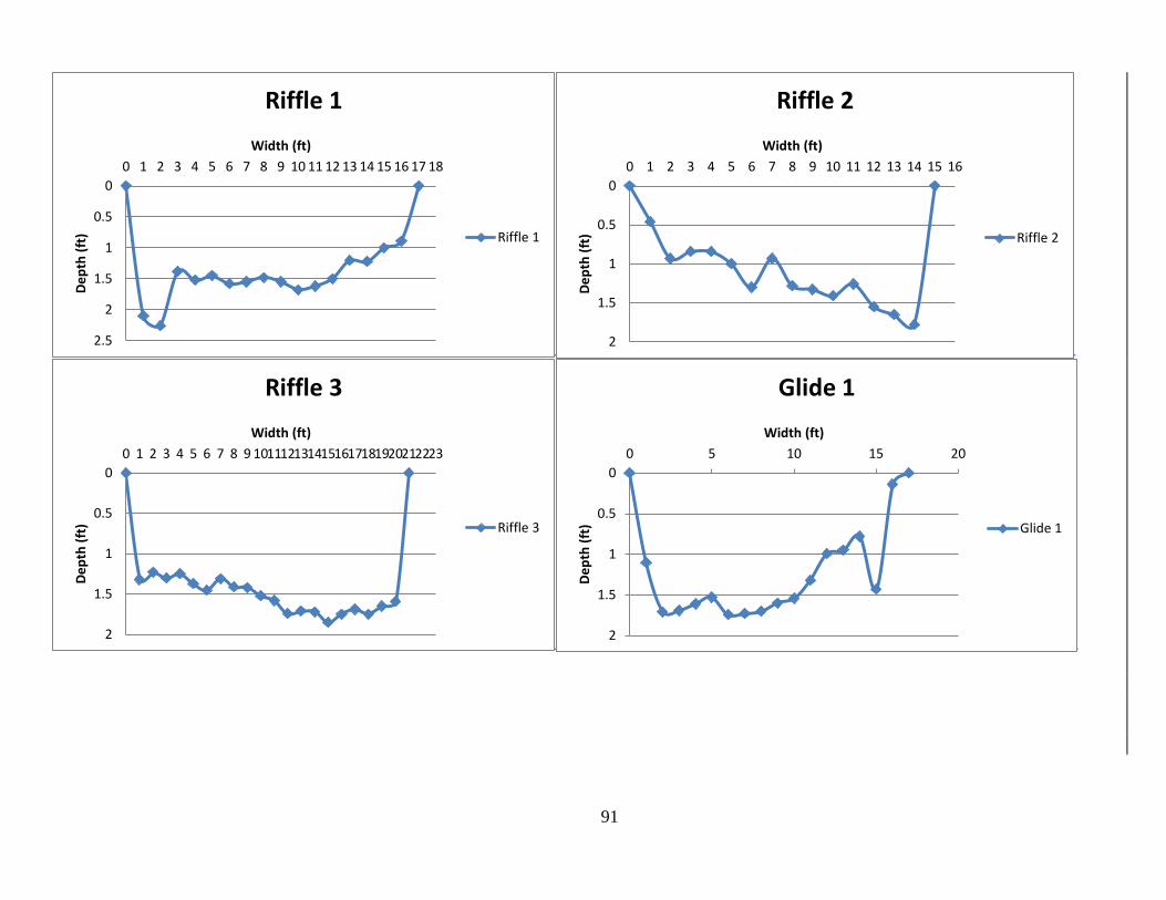
91
0
0.5
1
1.5
2
2.5
0 1 2 3 4 5 6 7 8 9 10 11 12 13 14 15 16 17 18
Dept
h (ft
)
Width (ft)
Riffle 1
Riffle 1
0
0.5
1
1.5
2
0 1 2 3 4 5 6 7 8 9 10 11 12 13 14 15 16
Dept
h (ft
)
Width (ft)
Riffle 2
Riffle 2
0
0.5
1
1.5
2
0 1 2 3 4 5 6 7 8 9 1011121314151617181920212223
Dept
h (ft
)
Width (ft)
Riffle 3
Riffle 3
0
0.5
1
1.5
2
0 5 10 15 20
Dept
h (ft
)
Width (ft)
Glide 1
Glide 1

92
0
0.5
1
1.5
2
2.5
0 5 10 15
Dept
h (ft
)
Width (ft)
Glide 2
Glide 2
0
0.5
1
1.5
2
2.5
3
3.5
4
0 5 10 15
Dept
h (ft
)
Width (ft)
Glide 3
Glide 3
0
0.5
1
1.5
2
2.5
0 5 10 15 20 25
Dept
h (ft
)
Width (ft)
Run 1
Run 1
0
0.5
1
1.5
2
2.5
3
0 5 10 15 20
Dept
h (ft
)
Width (ft)
Run 2
Run 2

93
0
0.5
1
1.5
2
2.5
3
3.5
0 5 10 15
Dept
h (ft
)
Width (ft)
Run 3
Run 3
0
1
2
3
4
5
0 5 10 15 20 25 30
Dept
h (ft
)
Width (ft)
Pool 1
Pool 1

94
0
0.5
1
1.5
2
2.5
3
3.5
0 5 10 15
Dept
h (ft
)
Width (ft)
Pool 2
Pool 2
0
1
2
3
4
5
6
0 5 10 15 20
Dept
h (ft
)
Width (ft)
Pool 3
Pool 3
0
0.5
1
1.5
2
2.5
0 1 2 3 4 5 6 7 8 9 10 11 12 13 14 15 16 17 18
Dept
h (ft
)
Width (ft)
Riffle 1
Riffle 1
0
0.5
1
1.5
2
0 1 2 3 4 5 6 7 8 9 10 11 12 13 14 15 16
Dept
h (ft
)
Width (ft)
Riffle 2
Riffle 2

95
0
0.5
1
1.5
2
0 1 2 3 4 5 6 7 8 9 1011121314151617181920212223
Dept
h (ft
)
Width (ft)
Riffle 3
Riffle 3
0
0.5
1
1.5
2
0 5 10 15 20
Dept
h (ft
)
Width (ft)
Glide 1
Glide 1
0
0.5
1
1.5
2
2.5
0 5 10 15
Dept
h (ft
)
Width (ft)
Glide 2
Glide 2
0
0.5
1
1.5
2
2.5
3
3.5
4
0 5 10 15
Dept
h (ft
)
Width (ft)
Glide 3
Glide 3

96
0
0.5
1
1.5
2
2.5
0 5 10 15 20 25
Dept
h (ft
)
Width (ft)
Run 1
Run 1
0
0.5
1
1.5
2
2.5
3
0 5 10 15 20
Dept
h (ft
)
Width (ft)
Run 2
Run 2
0
0.5
1
1.5
2
2.5
3
3.5
0 5 10 15
Dept
h (ft
)
Width (ft)
Run 3
Run 3
0
1
2
3
4
5
0 5 10 15 20 25 30
Dept
h (ft
)
Width (ft)
Pool 1
Pool 1

97
0
0.5
1
1.5
2
2.5
3
3.5
0 5 10 15
Dept
h (ft
)
Width (ft)
Pool 2
Pool 2
0
1
2
3
4
5
6
0 5 10 15 20
Dept
h (ft
)
Width (ft) Pool 3
Pool 3


99
5 APPENDIX 2 RESTORATION DESIGN
This appendix contains reference material for the restoration designs presented in
Section 3 of this report.
5.1 Frog Ponds
Detail drawings of the two ponds to be constructed are provided. The drawings are given
with meter (m) units.

100
5.1.1 Pond #1

101
5.1.2 Pond #2

102
5.2 Diversion
5.2.1 Diversion Structure
5.3 Pump
Qcfs
S. Weightlbs/ft^3
Rft
WS. Slope(ft/ft)
Bankfull Shear Stresslbs/ft^2
Bankfull Shear Stresskg/m^2
Minmum Rock Sizem
Minmum Rock Sizeft
150 62.4 1.5 0.0066 0.62 0.03 0.01 0.02840 62.4 4 0.0069 1.72 0.07 0.18 0.60
Shear=Gamma*R*S
Rock Size
Rad of Curvature (RC) Bankfull Width (BFW) Bankfull Width (BFW) RC/BFW Departure Angle 20-Rc/W 3 Departure Angle 30-Rc/w 3 Departure Angle 20-Rc/W 5 Departure Angle 30-Rc/w 5ft ft m ft/ft90 30 9.1 3.00 1.00 0.67 1.10 0.90
Length (m) 9.13 6.17 10.05 8.22Length (ft) 30.0 20.2 33.0 27.0
Rad of Curvature (RC) Bankfull Width (BFW) Bankfull Width (BFW) RC/BFW Departure Angle 20-Rc/W 3 Departure Angle 30-Rc/w 3 Departure Angle 20-Rc/W 5 Departure Angle 30-Rc/w 5ft ft m ft/ft90 30 9.1 3.00 2.42 1.80 2.50 2.13
Spacing (m) 22.16 16.49 22.88 19.44Spacing (ft) 72.7 54.1 75.0 63.8
Angle from Bank to Invert2% to 7%
Vane Spacing
Vane Length

103
5.4 Pipe
Max Q Max P cfs psi 4.54 2.20
L (m) L (ft) top (OBJECT_ID) Top El. (ft) bottem (OBJECT_ID) Joint El. (ft) del (ft) slope n Diamter (in) Diameter (ft) Rad (ft)426.5 1398.92 538 5118.58904 1408 5113.517084 5.07196 0.003626 0.012 15 1.25 0.625
Pipe and Channel From diversion to below the house near the road
pipe section
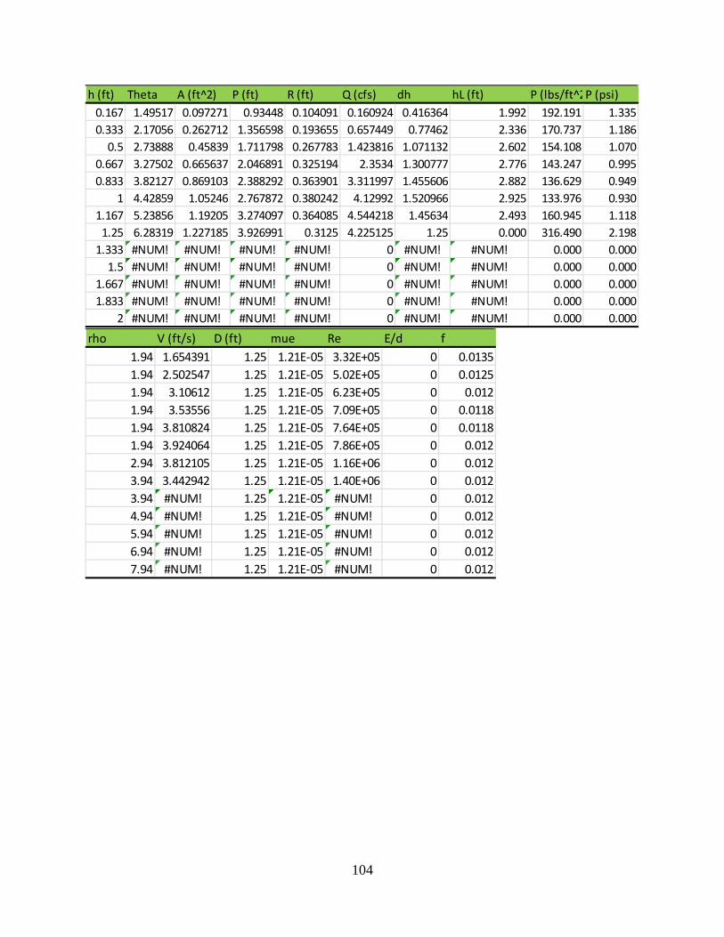
104
h (ft) Theta A (ft^2) P (ft) R (ft) Q (cfs) dh hL (ft) P (lbs/ft^2P (psi)0.167 1.49517 0.097271 0.93448 0.104091 0.160924 0.416364 1.992 192.191 1.3350.333 2.17056 0.262712 1.356598 0.193655 0.657449 0.77462 2.336 170.737 1.186
0.5 2.73888 0.45839 1.711798 0.267783 1.423816 1.071132 2.602 154.108 1.0700.667 3.27502 0.665637 2.046891 0.325194 2.3534 1.300777 2.776 143.247 0.9950.833 3.82127 0.869103 2.388292 0.363901 3.311997 1.455606 2.882 136.629 0.949
1 4.42859 1.05246 2.767872 0.380242 4.12992 1.520966 2.925 133.976 0.9301.167 5.23856 1.19205 3.274097 0.364085 4.544218 1.45634 2.493 160.945 1.118
1.25 6.28319 1.227185 3.926991 0.3125 4.225125 1.25 0.000 316.490 2.1981.333 #NUM! #NUM! #NUM! #NUM! 0 #NUM! #NUM! 0.000 0.000
1.5 #NUM! #NUM! #NUM! #NUM! 0 #NUM! #NUM! 0.000 0.0001.667 #NUM! #NUM! #NUM! #NUM! 0 #NUM! #NUM! 0.000 0.0001.833 #NUM! #NUM! #NUM! #NUM! 0 #NUM! #NUM! 0.000 0.000
2 #NUM! #NUM! #NUM! #NUM! 0 #NUM! #NUM! 0.000 0.000rho V (ft/s) D (ft) mue Re E/d f
1.94 1.654391 1.25 1.21E-05 3.32E+05 0 0.01351.94 2.502547 1.25 1.21E-05 5.02E+05 0 0.01251.94 3.10612 1.25 1.21E-05 6.23E+05 0 0.0121.94 3.53556 1.25 1.21E-05 7.09E+05 0 0.01181.94 3.810824 1.25 1.21E-05 7.64E+05 0 0.01181.94 3.924064 1.25 1.21E-05 7.86E+05 0 0.0122.94 3.812105 1.25 1.21E-05 1.16E+06 0 0.0123.94 3.442942 1.25 1.21E-05 1.40E+06 0 0.0123.94 #NUM! 1.25 1.21E-05 #NUM! 0 0.0124.94 #NUM! 1.25 1.21E-05 #NUM! 0 0.0125.94 #NUM! 1.25 1.21E-05 #NUM! 0 0.0126.94 #NUM! 1.25 1.21E-05 #NUM! 0 0.0127.94 #NUM! 1.25 1.21E-05 #NUM! 0 0.012
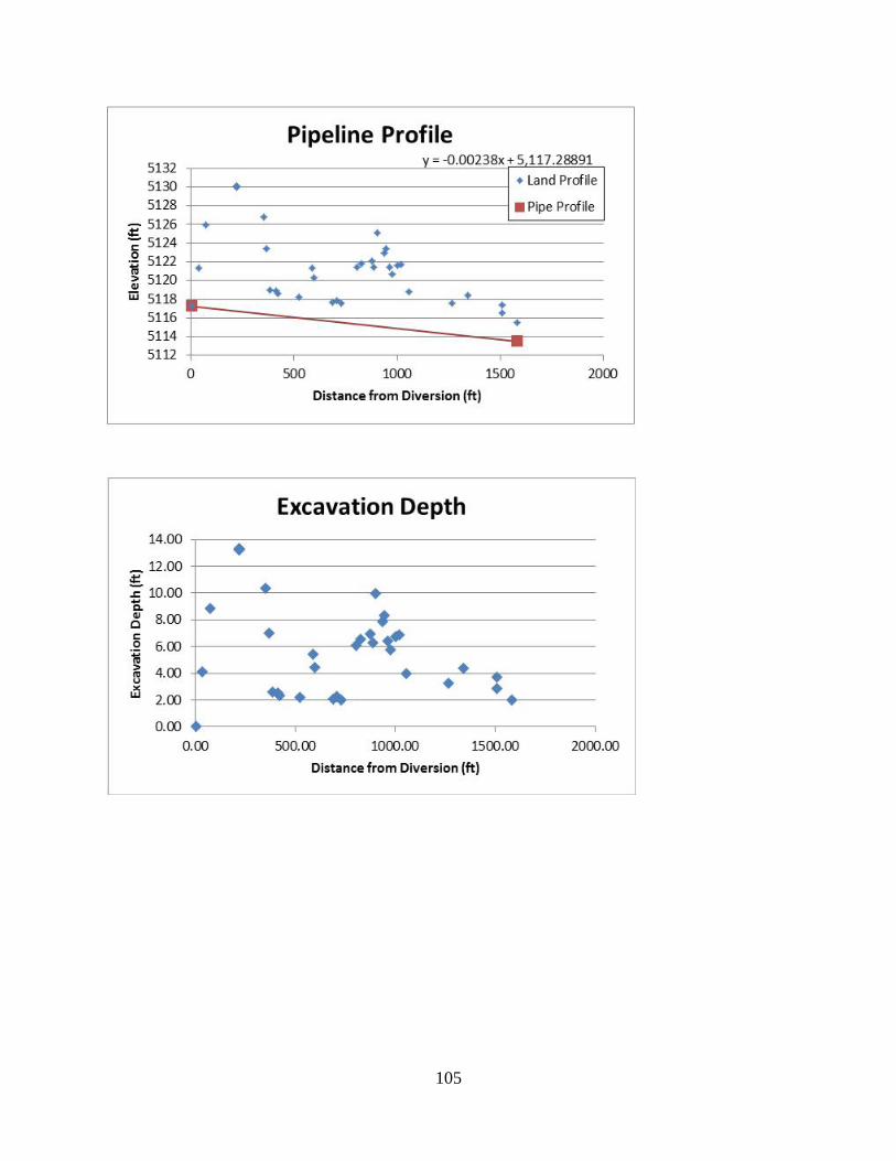
105

106
y = -0.00238x + 5,117.28891
51125114511651185120512251245126512851305132
0 500 1000 1500 2000
Elev
atio
n (ft
)
Distance from Diversion (ft)
Pipeline Profile
Land Profile
Pipe Profile
0.00
2.00
4.00
6.00
8.00
10.00
12.00
14.00
0.00 500.00 1000.00 1500.00 2000.00
Exca
vatio
n De
pth
(ft)
Distance from Diversion (ft)
Excavation Depth

107
5.5 Channel
y = -0.00238x + 5,117.28891
51125114511651185120512251245126512851305132
0 500 1000 1500 2000
Elev
atio
n (ft
)
Distance from Diversion (ft)
Pipeline Profile
Land Profile
Pipe Profile
0.00
2.00
4.00
6.00
8.00
10.00
12.00
14.00
0.00 500.00 1000.00 1500.00 2000.00
Exca
vatio
n De
pth
(ft)
Distance from Diversion (ft)
Excavation Depth

108
h (in) h (ft) S W (ft) A (ft)^2 P (ft) R (ft) V (ft/s) Q (ft^3/s)
4 0.333333 1.5 0.416667 4.75 0.087719298 0.46489 0.193704 8 0.666667 2 1 6 0.166666667 0.713159 0.713159 12 1 2.5 1.75 7.25 0.24137931 0.912894 1.597564 16 1.333333 3 2.666667 8.5 0.31372549 1.087227 2.899271 20 1.666667 3.5 3.75 9.75 0.384615385 1.245388 4.670205 24 2 4 5 11 0.454545455 1.392104 6.960522
L (m) L (ft) top (OBJECT_ID) Top El. (ft) bottem (OBJECT_ID) Bottom El. (ft) del (ft) slope n b (ft) T (ft) y (ft) z1 (ft) z2 (ft)515.82 1691.89 1408 5113.517084 2469 5102.95264 10.5644 0.006244 0.05 1 4 2 0.75 0.75
Channel Section

109
5.6 Cost Estimates

110
Rock Dia (ft) vol (ft^3)/rock # of rocks* Vol total (ft^3) lb of Rock Tons of
Rock 3 14.14 140 1979.2 321106 160.6
Rock (ton) Ton/Load Loads $/ton hr/trip $/hr $ Rock $ Delivery $ TotalDouble* 160.6 38 4.23 25.00$ 2.5 140.00$ 4,013.82$ 1,478.78$ 5,492.60$ Single* 160.6 22 7.30 25.00$ 2.5 120.00$ 4,013.82$ 2,189.36$ 6,203.18$ *Double needs 120 feet to get turned around
Rock (ton) Ton/Load Loads $/ton hr/trip $/hr $ Rock $ Delivery $ TotalDouble* 552 38 14.52 25 2.5 140 13,790.40$ 5,080.67$ 18,871.07$ Single* 552 22 25.07 25 2.5 120 13,790.40$ 7,522.04$ 21,312.44$ *Double needs 120 feet to get turned around
Rock (ton) Ton/Load Loads $/ton hr/trip $/hr $ Rock $ Delivery $ TotalDouble* 552 38 14.52 17 2.5 140 9,377.47$ 5,080.67$ 14,458.15$ Single* 552 22 25.07 17 2.5 120 9,377.47$ 7,522.04$ 16,899.51$ *Double needs 120 feet to get turned around
Rock (ton) Ton/Load Loads $/ton hr/trip $/hr $ Rock $ Delivery $ TotalDouble* 136 38 3.58 17 2.5 140 2,312.00$ 1,252.63$ 3,564.63$ Single* 136 22 6.18 17 2.5 120 2,312.00$ 1,854.55$ 4,166.55$ *Double needs 120 feet to get turned around
Rock for Stream Structures (Geneva Estimate) (< 3 ft diameter)
Wood for Fill () ()
Rock for Fill (Geneva Estimate) (< 3 ft diameter)
Rock for Fill (Geneva Estimate) (0.5 to 1 ft diameter)
Area Depth Wood Depth Rock Volume Wood Volume Rock W. Wood W. Rock(ft^2) (ft) (ft) (ft^3) (ft^3) (Tons) (Tons)
Fill Site 1 1000 2 2 2000 2000 40 162Fill Site 2 2000 2 2 4000 4000 80 324Plug Fill Site 3 400 2 2 800 800 16 65
Total 6800 6800 136 552
Fill Volume

111
REFERENCES
Thistle, Utah Landslide. (1983, April). Retrieved December 2012, from U.S. Geological Survey.
Binns, N. A. (1982). Habitat Quality Index Procedures Manual. Wyoming Game and Fish Department.
Buffington, M. D. (1998). Channel Processes, Classification, and Responce. River Ecology and Management.
Crocket, C. (2012). Columbia Spotted Frog Habitat Requirements. (J. Payne, Interviewer)
DWR, U. (n.d.). Fence Construction Specifications.
Hotchkiss, R. (2012). CEEN 635 Sediment Transport. Provo, Utah: Brigham Young University, Fullerton College of Engineering.
Michael M. Pollock, M. H. (2003). Hydrolic and Geomorphic Effects of Beaver Dams and Their Influence on Fishes.
Nielson, J. (2012). Mentor/ Corespondant. Utah, Springville: Utah Division of Wildlife.
Paige, C. (2008). A Landowner's Guide to Wildlife Freindly Fences. Helena, MT: Montana Fish and Wildlife Parks.
Peterson, D. R. (1998). A Review of the Habitat Requirements of the Columbia Spotted Frog in the Intermountain Region and Recommendations for the Restoration of Columbia Spotted Frog Habitat along the Middle Provo River. Pocotello, ID: Idaho State University - Dept of Biological Sciences.
Photography, U. D. (n.d.). Thistle, Utah.
Rosgen, D. (1997). A Geomorphological Approach to Restoration of Incised Rivers. Proceedings of the Conference on Management of Landscapes Disturbed by Channel Incision.
Rosgen, D. (2007, August). Part 654 - Stream Restoration Design/ Chapter 11: Rosgen Geomorphic Channel Design. Retrieved from NRCS eDirectives: http://directives.sc.egov.usda.gov/viewerFS.aspx?id=3491

112
Rosgen, D. (2012, June). Sun Valley Restoration Tour. Sun Valley , Idaho: Wildland Hydrology.
Rosgen, D. (n.d.). The Cross-Vane, W-Weir and J-Hook Vane Structures…Their. Retrieved January 2013, from Wildland Hydrology: http://www.wildlandhydrology.com/assets/cross-vane.pdf
Schumm, A. a. (1973). Implications of complex response of drainage systems for quaternary alluvial stratigraphy. Nature (Physical Science).
State of Utah Natural Resources - Wildlife Resources. (n.d.). Retrieved Dec 2012, from List of Fishes in Utah: http://dwrcdc.nr.utah.gov/rsgis2/Search/Display.asp?FlNm=gilacope
Tempus, World. (n.d.). Born with the epic of American Railroads. Retrieved December 2012, from http://www.worldtempus.com/en/brands/partner-brands/ball-watch/history/born-with-the-epic-of-american-railroads/
USGS, U. S. (n.d.). StreamStats. Retrieved May 2012, from http://water.usgs.gov/osw/streamstats/
Wilcox, P. (2012, August). Stream Restoration Workshop. Sediment Transport in Stream Assessment and Design. Logan, Utah: Utah State University.