Learning Key-Value Store Design

Stratos Idreos, Niv Dayan, Wilson Qin, Mali Akmanalp, Sophie Hilgard, Andrew Ross,James Lennon, Varun Jain, Harshita Gupta, David Li, Zichen Zhu

Harvard University

ABSTRACTWe introduce the concept of design continuums for the datalayout of key-value stores. A design continuum unifies majordistinct data structure designs under the same model. Thecritical insight and potential long-term impact is that suchunifying models 1) render what we consider up to now asfundamentally different data structures to be seen as“views”of the very same overall design space, and 2) allow “seeing”new data structure designs with performance properties thatare not feasible by existing designs. The core intuition be-hind the construction of design continuums is that all datastructures arise from the very same set of fundamental de-sign principles, i.e., a small set of data layout design con-cepts out of which we can synthesize any design that existsin the literature as well as new ones. We show how to con-struct, evaluate, and expand, design continuums and we alsopresent the first continuum that unifies major data structuredesigns, i.e., B+tree, Bεtree, LSM-tree, and LSH-table.

The practical benefit of a design continuum is that it cre-ates a fast inference engine for the design of data structures.For example, we can predict near instantly how a specific de-sign change in the underlying storage of a data system wouldaffect performance, or reversely what would be the optimaldata structure (from a given set of designs) given workloadcharacteristics and a memory budget. In turn, these prop-erties allow us to envision a new class of self-designing key-value stores with a substantially improved ability to adaptto workload and hardware changes by transitioning betweendrastically different data structure designs to assume a di-verse set of performance properties at will.

1. A VAST DESIGN SPACEKey-value stores are everywhere, providing the stor-

age backbone for an ever-growing number of diverse appli-cations. The scenarios range from graph processing in socialmedia [11, 18], to event log processing in cybersecurity [19],application data caching [71], NoSQL stores [78], flash trans-lation layer design [26], time-series management [51, 52], andonline transaction processing [31]. In addition, key-valuestores increasingly have become an attractive solution as

This is an extended version of a paper presented at CIDR 2019, the 9thBiennial Conference on Innovative Data Systems.

Read Memory

Update

Performance

Trade-offs

Data Structures

Key-Value StoresDatabases

Access PatternsHardwareCloud costs

K V K V K V…Table

TableLSM

Hash

B-Tree

Machine

GraphStore

Data

Learning

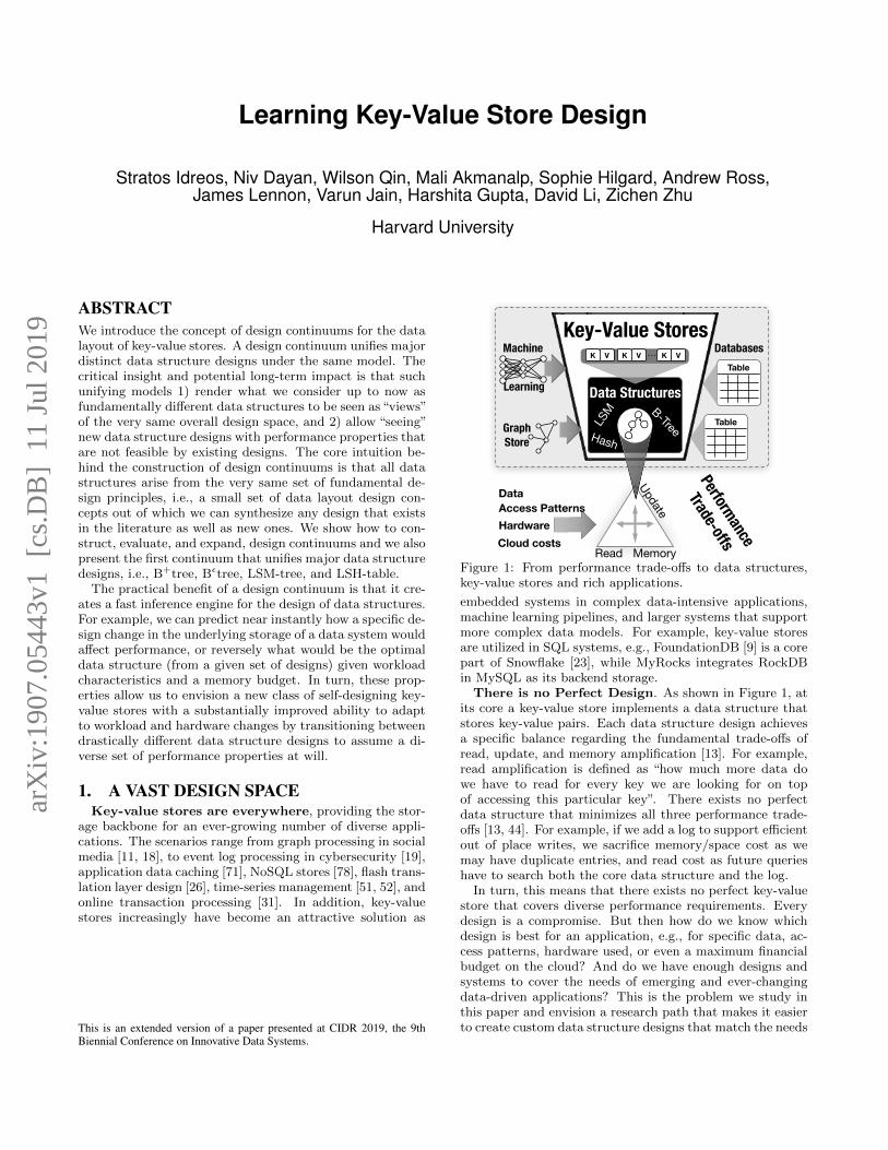
Figure 1: From performance trade-offs to data structures,key-value stores and rich applications.

embedded systems in complex data-intensive applications,machine learning pipelines, and larger systems that supportmore complex data models. For example, key-value storesare utilized in SQL systems, e.g., FoundationDB [9] is a corepart of Snowflake [23], while MyRocks integrates RockDBin MySQL as its backend storage.

There is no Perfect Design. As shown in Figure 1, atits core a key-value store implements a data structure thatstores key-value pairs. Each data structure design achievesa specific balance regarding the fundamental trade-offs ofread, update, and memory amplification [13]. For example,read amplification is defined as “how much more data dowe have to read for every key we are looking for on topof accessing this particular key”. There exists no perfectdata structure that minimizes all three performance trade-offs [13, 44]. For example, if we add a log to support efficientout of place writes, we sacrifice memory/space cost as wemay have duplicate entries, and read cost as future querieshave to search both the core data structure and the log.

In turn, this means that there exists no perfect key-valuestore that covers diverse performance requirements. Everydesign is a compromise. But then how do we know whichdesign is best for an application, e.g., for specific data, ac-cess patterns, hardware used, or even a maximum financialbudget on the cloud? And do we have enough designs andsystems to cover the needs of emerging and ever-changingdata-driven applications? This is the problem we study inthis paper and envision a research path that makes it easierto create custom data structure designs that match the needs

arX

iv:1

907.

0544

3v1

[cs

.DB

] 1

1 Ju

l 201

9

of new applications, hardware, and cloud pricing schemes.The Big Three. As of 2018, there are three predomi-

nant data structure designs for key-value stores to organizedata. To give an idea of the diverse design goals and per-formance balances they provide, we go briefly through theircore design characteristics. The first one is the B+tree [15].The prototypical B+tree design consists of a leaf level of in-dependent nodes with sorted key-value pairs (typically mul-tiple storage blocks each) and an index (logarithmic at thenumber of leaf nodes) which consists of nodes of fractionalcascading fence pointers with a large fanout. For example,B+tree is the backbone design of the BerkeleyDB key-valuestore [73], now owned by Oracle, and the backbone of theWiredTiger key-value store [94], now used as the primarystorage engine in MongoDB [72]. FoundationDB [9] also re-lies on a B+tree. Overall, B+tree achieves a good balancebetween read and write performance with a reasonable mem-ory overhead that is primarily due to its fill factor in eachnode (typically 50%) and the auxiliary internal index nodes.

In the early 2000s, a new wave of applications emergedrequiring faster writes, while still giving good read perfor-mance. At the same time, the advent of flash-based SSDshas made write I/Os 1-2 orders of magnitude costlier thanread I/Os [1]. These workload and hardware trends ledto two data structure design decisions for key-value stores:1) buffering new data in memory, batching writes in sec-ondary storage, and 2) avoiding global order maintenance.This class of designs was pioneered by the Log-StructuredMerge Tree (LSM-tree) [74] which partitions data tem-porally in a series of increasingly larger levels. Each key-value entry enters at the very top level (the in-memory writebuffer) and is sort-merged at lower levels as more data ar-rives. In-memory structures such as Bloom filters, fencepointers and Tries help filter queries to avoid disk I/O [24,99]. This design has been adopted in numerous industrialsettings including LevelDB [35] and BigTable [21] at Google,RocksDB [32] at Facebook, Cassandra [60], HBase [38] andAccumulo [8] at Apache, Voldemort [65] at LinkedIn, Dy-namo [29] at Amazon, WiredTiger [94] at MongoDB, andbLSM [84] and cLSM [34] at Yahoo, and more designs in re-search such as SlimDB [79], WiscKey [68], Monkey [24, 25],Dostoevsky [27], and LSM-bush [28]. Relational databasessuch as MySQL and SQLite4 support this design too bymapping primary keys to rows as values. Overall, LSM-tree-based designs achieve better writes than B+tree-baseddesigns but they typically give up some read performance(e.g., for short-range queries) given that we have to look fordata through multiple levels, and they also give up somememory amplification to hold enough in-memory filters tosupport efficient point queries. Crucial design knobs, suchas fill factor for B+tree and size ratio for LSM-tree, definethe space amplification relationship among the two designs.

More recently, a third design emerged for applications thatrequire even faster ingestion rates. The primary data struc-ture design decision was to drop order maintenance. Dataaccumulates in an in-memory write buffer. Once full, it ispushed to secondary storage as yet another node of an ever-growing single level log. An in-memory index, e.g., a hash ta-ble, allows locating any key-value pair easily while the log isperiodically merged to enforce an upper bound on the num-ber of obsolete entries. This Log-Structured Hash-table(LSH-table) is employed by BitCask [86] at Riak, Sparkey[88] at Spotify, FASTER [20] at Microsoft, and many more

systems in research [80, 64, 2]. Overall, LSH-table achievesexcellent write performance, but it sacrifices read perfor-mance (for range queries), while the memory footprint isalso typically higher since now all keys need to be indexedin-memory to minimize I/O needs per key.

The Practical Problem. While key-value stores con-tinue to be adopted by an ever-growing set of applications,each application has to choose among the existing designswhich may or may not be close to the ideal performancethat could be achieved for the specific characteristics of theapplication. This is a problem for several increasingly press-ing reasons. First, new applications appear many of whichintroduce new workload patterns that were not typical be-fore. Second, existing applications keep redefining their ser-vices and features which affects their workload patterns di-rectly and in many cases renders the existing underlyingstorage decisions sub-optimal or even bad. Third, hardwarekeeps changing which affects the CPU/bandwidth/latencybalance. Across all those cases, achieving maximum perfor-mance requires low-level storage design changes. This boilsdown to the one size does not fit all problem, which holdsfor overall system design [90] and for the storage layer [13].

Especially in today’s cloud-based world, even designsslightly sub-optimal by 1% translate to a massive loss inenergy utilization and thus costs [57], even if the perfor-mance difference is not directly felt by the end users. Thisimplies two trends. First, getting as close to the optimaldesign is critical. Second, the way a data structure designtranslates to cost needs to be embedded in the design pro-cess as it is not necessarily about achieving maximum querythroughput, but typically a more holistic view of the de-sign is needed, including the memory footprint. Besides,the cost policy varies from one cloud provider to the next,and even for the same provider it may vary over time. Forexample, Amazon AWS charges based on CPU and memoryfor computation resources, and based on volume size, re-served throughput, and I/O performed for networked stor-age. Google Cloud Platform, while charging similarly forcomputation, only charges based on volume size for net-worked storage. This implies that the optimal data structure1) is different for different cloud providers where the key-value store is expected to run, and 2) can vary over timefor the same cloud provider even if the application itself andunderlying hardware stay the same.

The Research Challenge. The long-term challenge iswhether we can easily or even automatically find the op-timal storage design for a given problem. This has beenrecognized as an open problem since the early days of com-puter science. In his seminal 1978 paper, Robert Tarjanincludes this problem in his list of the five major challengesfor the future (which also included P Vs NP ) [91]: “Is therea calculus of data structures by which one can choose theappropriate data representation and techniques for a givenproblem?”. We propose that a significant step toward a so-lution includes dealing with the following two challenges:

1) Can we know all possible data structure designs?

2) Can we compute the performance of any design?

Toward an Answer to Challenge 1. We made a steptoward the first challenge by introducing the design spaceof data structures supporting the key-value model [45]. Thedesign space is defined by all designs that can be described

design space

fanout

filter bits

buffer size

merge policy…

Design Primitives

data structures design continuum

LSM

B-tre

e

TGCF

YTKVG

OGOQT[

&CVC�UVTWEVWTG�FGUKIPU�CTG�FGTKXGF�CU�EQODKPCVKQPU�QH�HWPFCOGPVCN�FGUKIP�RTKOKVKXGU

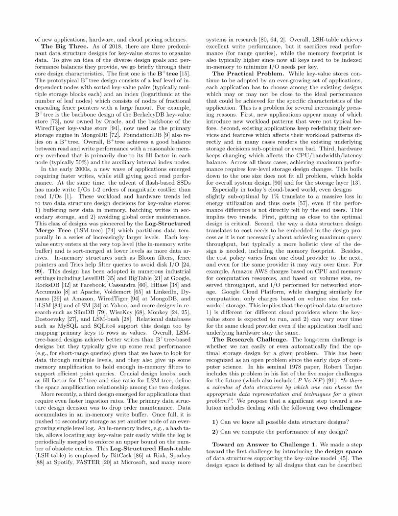
Figure 2: From data layout design principles to the de-sign space of possible data structures, where design continu-ums can be observed to help navigate performance trade-offsacross diverse data structure designs.

as combinations and tunings of the “first principles of datalayout design”. A first principle is a fundamental design con-cept that cannot be broken into additional concepts, e.g.,fence pointers, links, and temporal partitioning. The intu-ition is that, over the past several decades, researchers haveinvented numerous fundamental design concepts such thata plethora of new valid designs with interesting propertiescan be synthesized out of those [45].

As an analogy consider the periodic table of elementsin chemistry; it sketched the design space of existing ele-ments based on their fundamental components, and allowedresearchers to predict the existence of unknown, at the time,elements and their properties, purely by the structure of thedesign space. In the same way, we created the periodictable of data structures [44] which describes more datastructure designs than stars on the sky and can be used asa design and new data structure discovery guide.

Naturally, a design space does not necessarily describe“allpossible data structures”; a new design concept may be in-vented and cause an exponential increase in the number ofpossible designs. However, after 50 years of computer sci-ence research, the chances of inventing a fundamentally newdesign concept have decreased exponentially; many excitinginnovations, in fact, come from utilizing a design conceptthat, while known, it was not explored in a given contextbefore and thus it revolutionizes how to think about a prob-lem. Using Bloom filters as a way to filter accesses in storageand remote machines, scheduling indexing construction ac-tions lazily [41], using ML models to guide data access [59],storage [50] and other system components [58], can all bethought of as such examples. Design spaces that cover largefundamental sets of concepts can help accelerate progresswith figuring out new promising directions, and when newconcepts are invented they can help with figuring out thenew possible derivative designs.

Toward an Answer to Challenge 2. The next pieceof the puzzle is to investigate if we can make it easy to com-pute the performance properties of any given data structuredesign. With the Data Calculator we introduced the idea oflearned cost models [45] which allow learning the costsof fundamental access patterns (random access, scan, sortedsearch) out of which we can synthesize the costs of complexalgorithms for a given data structure design. These costscan, in turn, be used by machine learning algorithms thatiterate over machine generated data structure specifications

to label designs, and to compute rewards, deciding which de-sign specification to try out next. Early results using geneticalgorithms show the strong potential of such approaches [42].However, there is still an essential missing link; given the factthat the design space size is exponential in the number ofdesign principles (and that it will likely only expand overtime), such solutions cannot find optimal designs in feasibletime, at least not with any guarantee, leaving valuable per-formance behind [57]. This is the new problem we attack inthis paper: Can we develop fast search algorithms that au-tomatically or interactively help researchers and engineersfind a close to optimal data structure design for a key-valuestore given a target workload and hardware environment?

Design Continuums. Like when designing any algo-rithm, the key ingredient is to induce domain-specific knowl-edge. Our insight is that there exist“design continuums”em-bedded in the design space of data structures. An intuitiveway to think of design continuums is as a performance hy-perplane that connects a specific subset of data structuresdesigns. Design continuums are effectively a projection ofthe design space, a “pocket” of designs where we can iden-tify unifying properties among its members. Figure 2 givesan abstract view of this intuition; it depicts the design spaceof data structures where numerous possible designs can beidentified, each one being derived as a combination of a smallset of fundamental design primitives and performance con-tinuums can be identified for subsets of those structures.

1. We introduce design continuums as subspaces of thedesign space which connect more than one design. Adesign continuum has the crucial property that it cre-ates a continuous performance tradeoff for fundamen-tal performance metrics such as updates, inserts, pointreads, long-range and short-range scans, etc.

2. We show how to construct continuums using few designknobs. For every metric it is possible to produce aclosed-form formula to quickly compute the optimaldesign. Thus, design continuums enable us to knowthe best key-value store design for a given workloadand hardware.

3. We present a design continuum that connects majorclasses of modern key-value stores including LSM-tree,Bεtree, and B+tree.

4. We show that for certain design decisions key-valuestores should still rely on learning as it is hard (per-haps even impossible) to capture them in a continuum.

5. We present the vision of self-designing key-value stores,which morph across designs that are now considered asfundamentally different.

Inspiration. Our work is inspired by numerous effortsthat also use first principles and clean abstractions to un-derstand a complex design space. John Ousterhout’s projectMagic allows for quick verification of transistor designs sothat engineers can easily test multiple designs synthesizedby basic concepts [75]. Leland Wilkinson’s “grammar ofgraphics” provides structure and formulation on the massiveuniverse of possible graphics [93]. Timothy G. Mattson’swork creates a language of design patterns for parallel algo-rithms [70]. Mike Franklin’s Ph.D. thesis explores the pos-sible client-server architecture designs using caching based

replication as the main design primitive [33]. Joe Heller-stein’s work on Generalized Search Trees makes it easy todesign and test new data structures by providing templateswhich expose only a few options where designs need to dif-fer [39, 6, 7, 54, 53, 55, 56]. S. Bing Yao’s [98] and StefanManegold’s [69] work on generalized hardware conscious costmodels showed that it is possible to synthesize the costs ofcomplex operations from basic access patterns. Work ondata representation synthesis in programming languages en-ables synthesis of representations out of small sets of (3-5)existing data structures [81, 82, 22, 87, 85, 36, 37, 67, 89].

2. DESIGN CONTINUUMSWe now describe how to construct a design continuum.

2.1 From B+tree to LSM-treeWe first give an example of a design continuum that con-

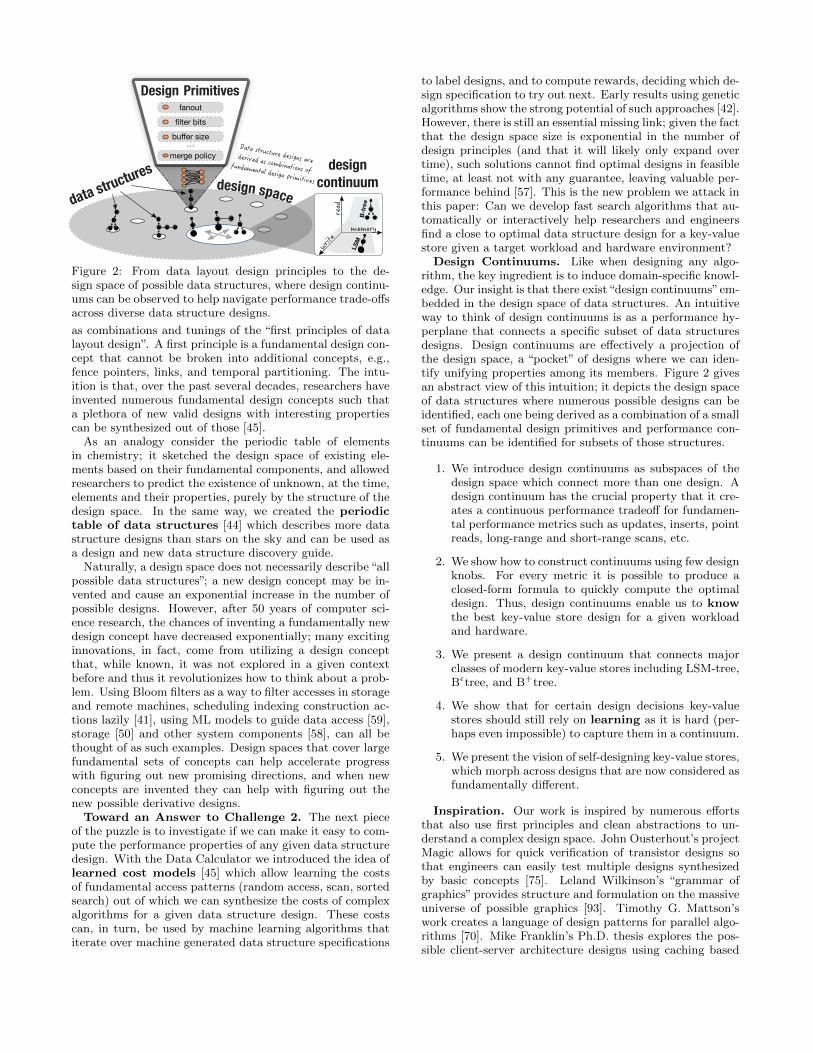
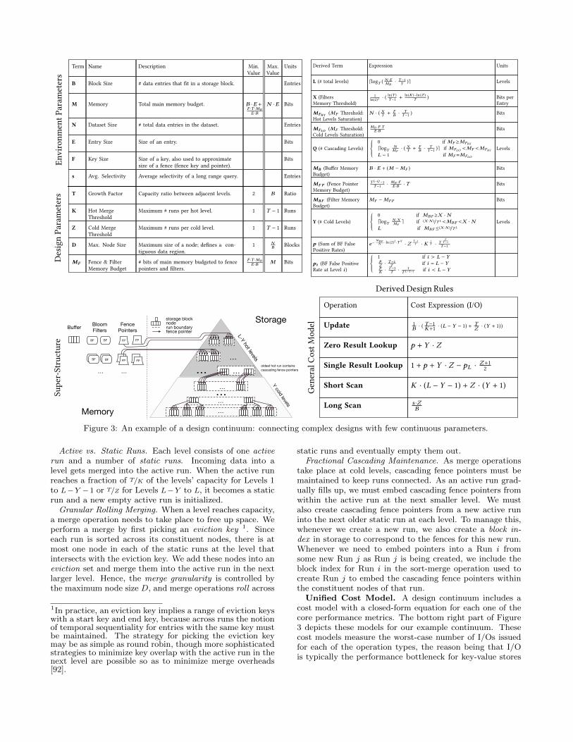
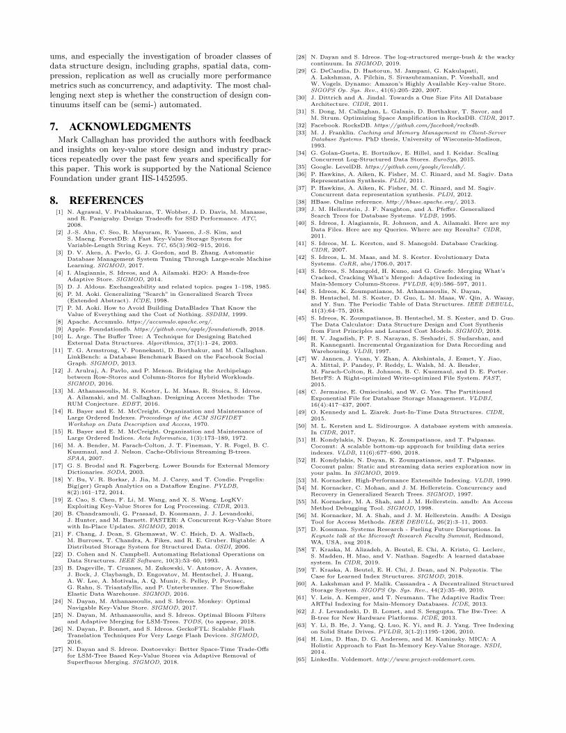
nects diverse designs including Tiered LSM-tree [46, 24, 60],Lazy Leveled LSM-tree [27], Leveled LSM-tree [74, 24, 32,35], COLA [16, 48], FD-tree [63], Bεtree [17, 10, 16, 47, 48,76], and B+tree [14]. The design continuum can be thoughtof as a super-structure that encapsulates all those designs.This super-structure consists of L levels where the larger Ylevels are cold and the smaller L − Y levels are hot. Hotlevels use in-memory fence pointers and Bloom filters to fa-cilitate lookups, whereas cold levels apply fractional cascad-ing to connect runs in storage. Each level contains one ormore runs, and each run is divided into one or more con-tiguous nodes. There is a write buffer in memory to ingestapplication updates and flush to Level 1 when it fills up.This overall abstraction allows instantiating any of the datastructure designs in the continuum. Figure 3 formalizes thecontinuum and the super-structure is shown at the bottomleft. For reference, we provide several examples of super-structure instantiations in Appendix A and Figure 12.

Environmental Parameters. The upper right table inFigure 3 opens with a number of environmental parameterssuch as dataset size, main memory budget, etc. which areinherent to the application and context for which we wantto design a key-value store.

Design Parameters. The upper right table in Figure 3further consists of five continuous design knobs which havebeen chosen as the smallest set of movable design abstrac-tions that we could find to allow differentiating among thetarget designs in the continuum. The first knob is the growthfactor T between the capacities of adjacent levels of thestructure (e.g., “fanout” for B+tree or “size ratio” for LSM-tree). This knob allows us to control the super-structure’sdepth. The second knob is the hot merge threshold K, whichis defined as the maximum number of independent sortedpartitions (i.e., runs) at each of Levels 1 to L− Y − 1 (i.e.,all hot levels but the largest) before we trigger merging. Thelower we set K, the more greedy merge operations becometo enforce fewer sorted runs at each of these hot levels. Sim-ilarly, the third knob is the cold merge threshold Z and isdefined as the maximum number of runs at each of LevelsL − Y to L (i.e., the largest hot level and all cold levels)before we trigger merging. The node size D is the maximalsize of a contiguous data region (e.g., a “node” in a B+treeor “SSTable” in an LSM-tree) within a run. Finally, thefence and filters memory budget MF controls the amountof the overall memory that is allocated for in-memory fencepointers and Bloom filters.

Setting the domain of each parameter is a critical partof crafting a design continuum so we can reach the targetdesigns and correct hybrid designs. Figure 3 describes howeach design parameter in the continuum may be varied. Forexample, we set the maximum value for the size ratio T tobe the block size B. This ensures that when fractional cas-cading is used at the cold levels, a parent block has enoughspace to store pointers to all of its children. As another ex-ample, we observe that a level can have at most T − 1 runsbefore it runs out of capacity and so based on this observa-tion we set the maximum values of K and Z to be T − 1.

Design Rules: Forming the Super-structure. Thecontinuum contains a set of design rules, shown on the up-per right part of Figure 3. These rules enable instantiatingspecific designs by deterministically deriving key design as-pects. Below we describe the design rules in detail.

Exponentially Increasing Level Capacities. The levels’ ca-pacities grow exponentially by a factor of T starting withthe write buffer’s capacity. As a result, the overall numberof levels L grows logarithmically with the data size.

Fence Pointers & Bloom Filters. Our design allocatesmemory for fence pointers and Bloom filters from smaller tolarger levels based on the memory budget assigned by theknob MF . Specifically, we first compute Q as the numberof levels for which there is not enough memory for havingboth Bloom filters and fence pointers. We then assign thememory budget MF for fence pointers to as many levels asthere is enough memory for. This is shown by the Equa-tion for the fence pointers budget MFP in Figure 3. Theremaining portion of MF after fence pointers is assigned toa Bloom filters memory budget MBF . This can also be donein the reverse way when one designs a structure, i.e., we candefine the desired write buffer budget first and then give theremaining from the total memory budget to filters and fencepointers.

Optimal Bloom Filter Allocation Across Levels. The con-tinuum assigns exponentially decreasing false positive rates(FPRs) to Bloom filters at smaller levels, as this approachwas shown to minimize the sum of their false positive ratesand thereby minimize point read cost [24]. In Figure 3, weexpress the FPR assigned to Level i as pi and give corre-sponding equations for how to set pi optimally with respectto the different design knobs.

Hot vs. Cold Levels. Figure 3 further shows how to com-pute the number of cold levels Y for which there is not suf-ficient memory for Bloom filters. The derivation for Y is interms of a known threshold X for when to drop a filter fora level and instead use that memory for filters at smallerlevels to improve performance [27]. Note that Y is eitherequal to Q or larger than it by at most one. We deriveMFHI as the amount of memory above which all levels arehot (i.e., Y = 0). We also set a minimum memory require-ment MFLO on MF to ensure that there is always enoughmemory for fence pointers to point to Level 1.

Fractional Cascading for Cold Levels. We use fractionalcascading to connect data at cold levels to the structure,to address the issue of not having enough memory to pointto them using in-memory fence pointers. For every blockwithin a run at a cold level, we embed a “cascading” fencepointer within the next younger run along with the smallestkey in the target block. This allows us to traverse cold levelswith one I/O for each run by following the correspondingcascading fence pointers to reach the target key range.

Envi

ronm

entP

aram

eter

sD

esig

nPa

ram

eter

sTerm Name Description Min.

ValueMax.Value

Units

B Block Size # data entries that �t in a storage block. Entries

M Memory Total main memory budget. B ·E +F ·T ·MB

E ·BN ·E Bits

N Dataset Size # total data entries in the dataset. Entries

E Entry Size Size of an entry. Bits

F Key Size Size of a key, also used to approximatesize of a fence (fence key and pointer).

Bits

s Avg. Selectivity Average selectivity of a long range query. Entries

T Growth Factor Capacity ratio between adjacent levels. 2 B Ratio

K Hot MergeThreshold

Maximum # runs per hot level. 1 T � 1 Runs

Z Cold MergeThreshold

Maximum # runs per cold level. 1 T � 1 Runs

D Max. Node Size Maximum size of a node; de�nes a con-tiguous data region.

1 NB Blocks

MF Fence & FilterMemory Budget

# bits of main memory budgeted to fencepointers and �lters.

F ·T ·MBE ·B M Bits

Derived Term Expression Units

L (# total levels) dlogT ( N ·EMB· T�1

T )e Levels

X (FiltersMemory Threshold)

1ln(2)2 · ( ln(T )

T�1 +ln(K )�ln(Z )

T ) Bits perEntry

MFH I (MF Threshold:Hot Levels Saturation)

N · ( XT +

FB · T

T�1 ) Bits

MFLO (MF Threshold:Cold Levels Saturation)

MB ·F ·TE ·B Bits

Q (# Cascading Levels)8>><>>:

0 if MF �MFH I

dlogTN

MF· ( X

T +FB · T

T�1 )e if MFLO <MF <MFH I

L � 1 if MF =MFLO

Levels

MB (Bu�er MemoryBudget)

B · E + (M �MF ) Bits

MF P (Fence PointerMemory Budget)

T L�Q �1T�1 · MB ·F

E ·B ·T Bits

MBF (Filter MemoryBudget)

MF �MF P Bits

Y (# Cold Levels)8>><>>:

0 if MBF �X · NdlogT

N ·XMFe if (X ·N )/T L <MBF <X · N

L if MBF (X ·N )/T L

Levels

p (Sum of BF FalsePositive Rates)

e�MBF

N ·ln (2)2 ·T Y · Z T�1T · K 1

T · TT

T�1T�1

pi (BF False PositiveRate at Level i )

8>><>>:1 if i > L � YpZ · T�1

T if i = L � YpK · T�1

T · 1T L�Y�i if i < L � Y

Derived Design Rules

Supe

r-St

ruct

ure

…

Buffer BloomFilters

Fence Pointers

Memory

Storage

FPBF

FPFP

BFBF BFBF …

……

…

…

…

noderun boundaryfence pointer

storage block

FPFP

…

L-Y hot levels

Y cold levels

FPBF

…oldest hot run containscascading fence pointers

Operation Cost Expression (I/O)

Update 1B · (

T�1K+1 · (L � Y � 1) + T

Z · (Y + 1))

Zero Result Lookup p + Y · Z

Single Result Lookup 1 + p + Y · Z � pL · Z+12

Short Scan K · (L � Y � 1) + Z · (Y + 1)

Long Scan s ·ZB

Gene

ralC

ostM

odel

Figure 3: An example of a design continuum: connecting complex designs with few continuous parameters.

Active vs. Static Runs. Each level consists of one activerun and a number of static runs. Incoming data into alevel gets merged into the active run. When the active runreaches a fraction of T/K of the levels’ capacity for Levels 1to L−Y − 1 or T/Z for Levels L−Y to L, it becomes a staticrun and a new empty active run is initialized.

Granular Rolling Merging. When a level reaches capacity,a merge operation needs to take place to free up space. Weperform a merge by first picking an eviction key 1. Sinceeach run is sorted across its constituent nodes, there is atmost one node in each of the static runs at the level thatintersects with the eviction key. We add these nodes into aneviction set and merge them into the active run in the nextlarger level. Hence, the merge granularity is controlled bythe maximum node size D, and merge operations roll across

1In practice, an eviction key implies a range of eviction keyswith a start key and end key, because across runs the notionof temporal sequentiality for entries with the same key mustbe maintained. The strategy for picking the eviction keymay be as simple as round robin, though more sophisticatedstrategies to minimize key overlap with the active run in thenext level are possible so as to minimize merge overheads[92].

static runs and eventually empty them out.Fractional Cascading Maintenance. As merge operations

take place at cold levels, cascading fence pointers must bemaintained to keep runs connected. As an active run grad-ually fills up, we must embed cascading fence pointers fromwithin the active run at the next smaller level. We mustalso create cascading fence pointers from a new active runinto the next older static run at each level. To manage this,whenever we create a new run, we also create a block in-dex in storage to correspond to the fences for this new run.Whenever we need to embed pointers into a Run i fromsome new Run j as Run j is being created, we include theblock index for Run i in the sort-merge operation used tocreate Run j to embed the cascading fence pointers withinthe constituent nodes of that run.

Unified Cost Model. A design continuum includes acost model with a closed-form equation for each one of thecore performance metrics. The bottom right part of Figure3 depicts these models for our example continuum. Thesecost models measure the worst-case number of I/Os issuedfor each of the operation types, the reason being that I/Ois typically the performance bottleneck for key-value stores

Para

met

ers

Met

rics

TermsDesigns Tiered LSM-

Tree [60,24, 25, 46]

Lazy LeveledLSM-Tree[27, 25]

Leveled LSM-Tree [35,

32, 24, 25]

COLA [16] FD-Tree [63] B� Tree [17, 16,47, 76, 10, 48]

B+Tree [14]

T (GrowthFactor)

[2, B] [2, B] [2, B] 2 [2, B] [2, B] B

K (Hot MergeThreshold)

T � 1 T � 1 1 1 1 1 1

Z (Cold MergeThreshold)

T � 1 1 1 1 1 1 1

D (Max.Node Size)

[1, NB ] [1, N

B ] [1, NB ] N

BNB 1 1

MF (Fence &Filter Mem.)

N · ( FB + 10) N · ( F

B + 10) N · ( FB + 10) F ·T ·MB

E ·BF ·T ·MB

E ·BF ·T ·MB

E ·BF ·T ·MB

E ·B

Update O ( LB ) O ( 1

B · (T + L)) O ( TB · L) O ( L

B ) O ( TB · L) O ( T

B · L) O (L)

Zero ResultLookup

O (T · e�MBF

N ) O (e� MBFN ) O (e� MBF

N ) O (L) O (L) O (L) O (L)

ExistingLookup

O (1+T · e �MBFN ) O (1) O (1) O (L) O (L) O (L) O (L)

Short Scan O (L · T ) O (1+T · (L � 1)) O (L) O (L) O (L) O (L) O (L)

Long Scan O (T · sB ) O ( s

B ) O ( sB ) O ( s

B ) O ( sB ) O ( s

B ) O ( sB )

Figure 4: Instances of the design continuum and examples of their derived cost metrics.

that store a larger amount of data than can fit in memory.2

For example, the cost for point reads is derived by addingthe expected number of I/Os due to false positives acrossthe hot levels (given by the Equation for p, the sum of theFPRs [27]) to the number of runs at the cold levels, sincewith fractional cascading we perform 1 I/O for each run.As another example, the cost for writes is derived by ob-serving that an application update gets copied on averageO(T/K) times at each of the hot levels (except the largest)and O(T/Z) times at the largest hot level and at each of thecold levels. We amortize by adding these costs and dividingby the block size B as a single write I/O copies B entriesfrom the original runs to the resulting run.

While our models in this work are expressed in terms ofasymptotic notations, we have shown in earlier work thatsuch models can be captured more precisely to reliably pre-dict worst-case performance [24, 27]. A central advantage ofhaving a set of closed-form set of models is that they allowus to see how the different knobs interplay to impact per-formance, and they reveal the trade-offs that the differentknobs control.

Overall, the choice of the design parameters and the deriva-tion rules represent the infusion of expert design knowledgein order to create a navigable design continuum. Specifi-cally, fewer design parameters (for the same target de-signs) lead to a cleaner abstraction which in turn makes iteasier to come up with algorithms that automatically findthe optimal design (to be discussed later on). We minimize

2Future work can also try to generate in-memory designcontinuums where we believe learned cost models that helpsynthesize the cost of arbitrary data structure designs canbe a good start [45].

the number of design parameters in two ways: 1) by addingdeterministic design rules which encapsulate expert knowl-edge about what is a good design, and 2) by collapsing morethan one interconnected design decisions to a single designparameter. For example, we used a single parameter forthe memory budget of Bloom filters and fence pointers aswe assume their co-existence since fence pointers accelerateboth point lookups and range queries, while Bloom filtersaccelerate point lookups exclusively. We specify a designstrategy that progressively adds more point query benefit asthe memory for fences and filters increases by prioritizingfence budget before filter budget at each level, accordinglyjointly budgeting fences and filters together as one designknob.

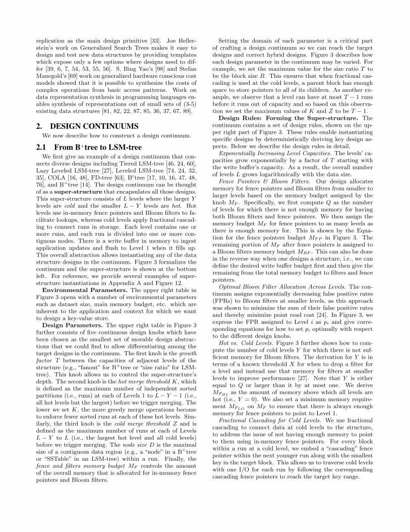
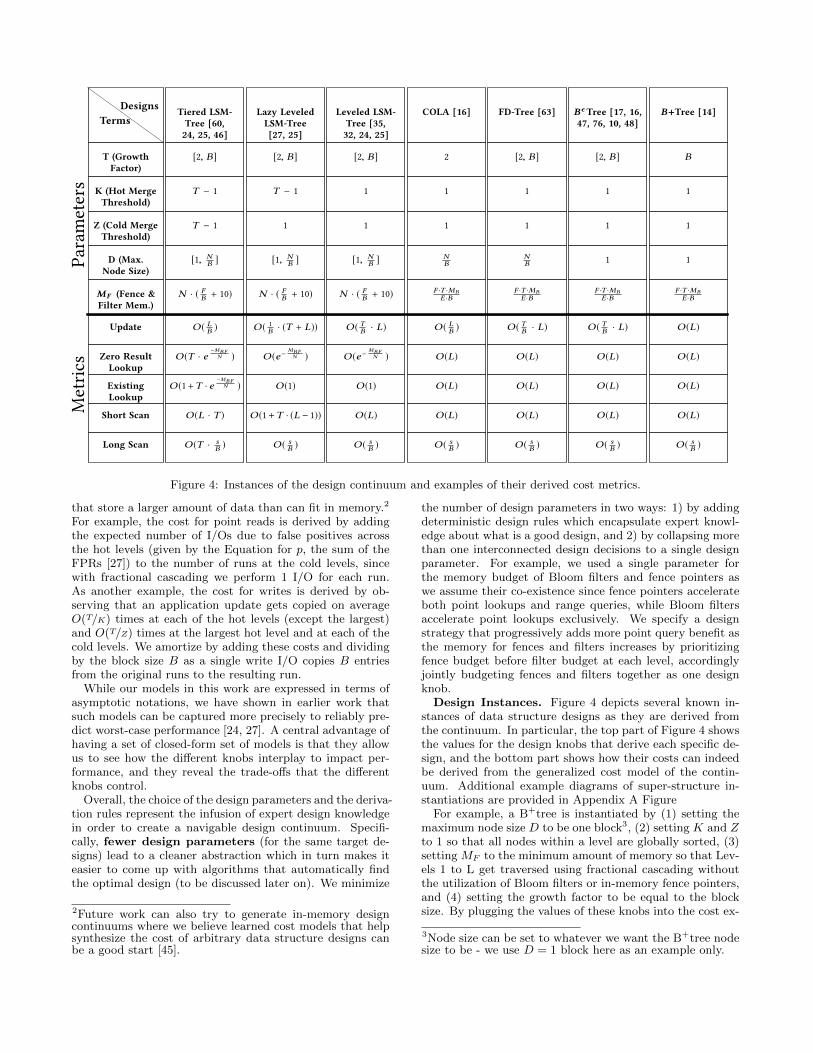
Design Instances. Figure 4 depicts several known in-stances of data structure designs as they are derived fromthe continuum. In particular, the top part of Figure 4 showsthe values for the design knobs that derive each specific de-sign, and the bottom part shows how their costs can indeedbe derived from the generalized cost model of the contin-uum. Additional example diagrams of super-structure in-stantiations are provided in Appendix A Figure

For example, a B+tree is instantiated by (1) setting themaximum node size D to be one block3, (2) setting K and Zto 1 so that all nodes within a level are globally sorted, (3)setting MF to the minimum amount of memory so that Lev-els 1 to L get traversed using fractional cascading withoutthe utilization of Bloom filters or in-memory fence pointers,and (4) setting the growth factor to be equal to the blocksize. By plugging the values of these knobs into the cost ex-

3Node size can be set to whatever we want the B+tree nodesize to be - we use D = 1 block here as an example only.

design space

LSMbLSM

designparameters

design continuum

Modelling

performance continuum

point read

Delete

Put

pareto curves

B-Tree

BeTreegrowth factor

filters memory

node size

levels

FGUKIP�RCTCO

GVGTU

EQODKPCVQTKCN�URCEG�QH�FGTKXGF�FGUKIPU

design rules

HKNVGT�RQUUKDNG�FGUKIPU

bound parameters

Figure 5: Constructing a design continuum: from design parameters to a performance hyperplane.

pressions, the well-known write and read costs for a B+treeof O(L) I/Os immediately follow.

As a second example, a leveled LSM-tree design is instan-tiated by (1) setting K and Z to 1 so that there is at mostone run at each level, and (2) assigning enough memoryto the knob MF to enable fence pointers and Bloom filters(with on average 10 bits per entry in the table) for all lev-els. We leave the knobs D and T as variables in this case asthey are indeed used by modern leveled LSM-tree designs tostrike different trade-offs. By plugging in the values for thedesign knobs into the cost models, we immediately obtainthe well-known costs for a leveled LSM-tree. For example,write cost simplifies to O(T ·L

B) as every entry gets copied

across O(L) levels and on average O(T ) times within eachlevel.

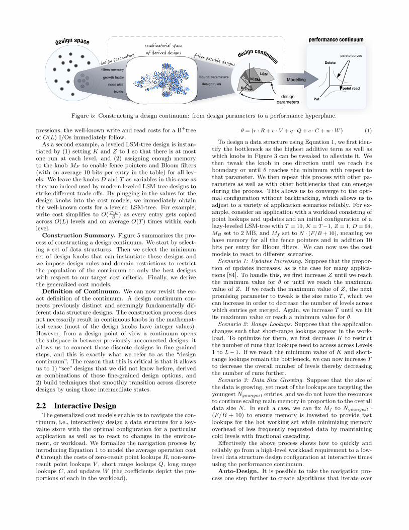
Construction Summary. Figure 5 summarizes the pro-cess of constructing a design continuum. We start by select-ing a set of data structures. Then we select the minimumset of design knobs that can instantiate these designs andwe impose design rules and domain restrictions to restrictthe population of the continuum to only the best designswith respect to our target cost criteria. Finally, we derivethe generalized cost models.

Definition of Continuum. We can now revisit the ex-act definition of the continuum. A design continuum con-nects previously distinct and seemingly fundamentally dif-ferent data structure designs. The construction process doesnot necessarily result in continuous knobs in the mathemat-ical sense (most of the design knobs have integer values).However, from a design point of view a continuum opensthe subspace in between previously unconnected designs; itallows us to connect those discrete designs in fine grainedsteps, and this is exactly what we refer to as the “designcontinuum”. The reason that this is critical is that it allowsus to 1) “see” designs that we did not know before, derivedas combinations of those fine-grained design options, and2) build techniques that smoothly transition across discretedesigns by using those intermediate states.

2.2 Interactive DesignThe generalized cost models enable us to navigate the con-

tinuum, i.e., interactively design a data structure for a key-value store with the optimal configuration for a particularapplication as well as to react to changes in the environ-ment, or workload. We formalize the navigation process byintroducing Equation 1 to model the average operation costθ through the costs of zero-result point lookups R, non-zero-result point lookups V , short range lookups Q, long rangelookups C, and updates W (the coefficients depict the pro-portions of each in the workload).

θ = (r ·R+ v · V + q ·Q+ c · C + w ·W ) (1)

To design a data structure using Equation 1, we first iden-tify the bottleneck as the highest additive term as well aswhich knobs in Figure 3 can be tweaked to alleviate it. Wethen tweak the knob in one direction until we reach itsboundary or until θ reaches the minimum with respect tothat parameter. We then repeat this process with other pa-rameters as well as with other bottlenecks that can emergeduring the process. This allows us to converge to the opti-mal configuration without backtracking, which allows us toadjust to a variety of application scenarios reliably. For ex-ample, consider an application with a workload consisting ofpoint lookups and updates and an initial configuration of alazy-leveled LSM-tree with T = 10, K = T−1, Z = 1, D = 64,MB set to 2 MB, and Mf set to N · (F/B + 10), meaning wehave memory for all the fence pointers and in addition 10bits per entry for Bloom filters. We can now use the costmodels to react to different scenarios.

Scenario 1: Updates Increasing. Suppose that the propor-tion of updates increases, as is the case for many applica-tions [84]. To handle this, we first increase Z until we reachthe minimum value for θ or until we reach the maximumvalue of Z. If we reach the maximum value of Z, the nextpromising parameter to tweak is the size ratio T , which wecan increase in order to decrease the number of levels acrosswhich entries get merged. Again, we increase T until we hitits maximum value or reach a minimum value for θ.

Scenario 2: Range Lookups. Suppose that the applicationchanges such that short-range lookups appear in the work-load. To optimize for them, we first decrease K to restrictthe number of runs that lookups need to access across Levels1 to L− 1. If we reach the minimum value of K and short-range lookups remain the bottleneck, we can now increase Tto decrease the overall number of levels thereby decreasingthe number of runs further.

Scenario 3: Data Size Growing. Suppose that the size ofthe data is growing, yet most of the lookups are targeting theyoungest Nyoungest entries, and we do not have the resourcesto continue scaling main memory in proportion to the overalldata size N . In such a case, we can fix Mf to Nyoungest ·(F/B + 10) to ensure memory is invested to provide fastlookups for the hot working set while minimizing memoryoverhead of less frequently requested data by maintainingcold levels with fractional cascading.

Effectively the above process shows how to quickly andreliably go from a high-level workload requirement to a low-level data structure design configuration at interactive timesusing the performance continuum.

Auto-Design. It is possible to take the navigation pro-cess one step further to create algorithms that iterate over

the continuum and independently find the best configura-tion. The goal is to find the best values for T , K, Z, D, andthe best possible division of a memory budget between MF

and MB . While iterating over every single configurationwould be intractable as it would require traversing everypermutation of the parameters, we can leverage the man-ner in which we constructed the continuum to significantlyprune the search space. For example, in Monkey [24], whenstudying a design continuum that contained only a limitedset of LSM-tree variants we observed that two of the knobshave a logarithmic impact on θ, particularly the size ratio Tand the memory allocation between Mb and Mf . For suchknobs, it is only meaningful to examine a logarithmic num-ber of values that are exponentially increasing, and so theirmultiplicative contribution to the overall search time is log-arithmic in their domain. While the continuum we showedhere is richer, by adding B-tree variants, this does not addsignificant complexity in terms of auto-design. The decisionto use cascading fence pointers or in-memory fence point-ers completely hinges on the allocation of memory betweenMF and MB , while the node size D adds one multiplicativelogarithmic term in the size of its domain.

2.3 Success CriteriaWe now outline the ideal success criteria that should guide

the construction of elegant and practically useful design con-tinuums in a principled approach.

Functionally Intact. All possible designs that can beassumed by a continuum should be able to correctly sup-port all operation types (e.g., writes, point reads, etc.). Inother words, a design continuum should only affect the per-formance properties of the different operations rather thanthe results that they return.

Pareto-Optimal. All designs that can be expressed shouldbe Pareto-optimal with respect to the cost metrics and work-loads desired. This means that there should be no two de-signs such that one of them is better than the other on oneor more of the performance metrics while being equal onall the others. The goal of only supporting Pareto-optimaldesigns is to shrink the size of the design space to the min-imum essential set of knobs that allow to control and nav-igate across only the best possible known trade-offs, whileeliminating inferior designs from the space.

Bijective. A design continuum should be a bijective (one-to-one) mapping from the domain of design knobs to theco-domain of performance and memory trade-offs. As withPareto-Optimality, the goal with bijectivity is to shrink adesign continuum to the minimal set of design knobs suchthat no two designs that are equivalent in terms of perfor-mance can be expressed as different knob configurations. Ifthere are multiple designs that map onto the same trade-off,it is a sign that the model is either too large and can becollapsed onto fewer knobs, or that there are core metricsthat we did not yet formalize, and that we should.

Diverse. A design continuum should enable a diverseset of performance properties. For Pareto-Optimal and bi-jective continuums, trade-off diversity can be measured andcompared across different continuums as the product of thedomains of all the design knobs, as each unique configurationleads to a different unique and Pareto-optimal trade-off.

Navigable. The time complexity required for navigat-ing the continuum to converge onto the optimal (or evennear-optimal) design should be tractable. With the Monkey

continuum, for example, we showed that it takes O(logT (N))

iterations to find the optimal design [24], and for Dosto-evsky, which includes more knobs and richer trade-offs, weshowed that it takes O(logT (N)3) iterations [27]. Measuringnavigability complexity in this way allows system designersfrom the onset to strike a balance between the diversity vs.the navigability of a continuum.

Layered. By construction, a design continuum has tostrike a trade-off between diversity and navigability. Themore diverse a continuum becomes through the introduc-tion of new knobs to assume new designs and trade-offs,the longer it takes to navigate it to optimize for differentworkloads. With that in mind, however, we observe that de-sign continuums may be constructed in layers, each of whichbuilds on top of the others. Through layered design, differ-ent applications may use the same continuum but choosethe most appropriate layer to navigate and optimize perfor-mance across. For example, the design continuum in Dos-toevsky [24] is layered on top of Monkey [27] by adding twonew knobs, K and Z, to enable intermediate designs be-tween tiering, leveling and lazy leveling. While Dostoevskyrequires O(logT (N)3) iterations to navigate the possible de-signs, an alternative is to leverage layering to restrict theknobs K and Z to both always be either 1 or T − 1 (i.e.,to enable only leveling and tiering) in order to project theMonkey continuum and thereby reduce navigation time toO(logT (N)). In this way, layered design enables continuumexpansion with no regret : we can continue to include new de-signs in a continuum to enable new structures and trade-offs,all without imposing an ever-increasing navigation penaltyon applications that need only some of the possible designs.

2.4 Expanding a Continuum:A Case-Study with LSH-table

We now demonstrate how to expand the continuum witha goal of adding a particular design to include certain per-formance trade-offs. The goal is to highlight the design con-tinuum construction process and principles.

Our existing continuum does not support the LSH-tabledata structure used in many key-value stores such as BitCask[86], FASTER [20], and others [2, 64, 80, 88, 95]. LSH-table achieves a high write throughout by logging entries instorage, and it achieves fast point reads by using a hash tablein memory to map every key to the corresponding entry inthe log. In particular, LSH-table supports writes in O(1/B)I/O, point reads in O(1) I/O, range reads in O(N) I/O, andit requires O(F · N) bits of main memory to store all keysin the hash table. As a result, it is suitable for write-heavyapplication with ample memory, and no range reads.

We outline the process of expanding our continuum inthree steps: bridging, patching, and costing.

Bridging. Bridging entails identifying the least numberof new movable design abstractions to introduce to a con-tinuum to assume a new design. This process involves threeoptions: 1) introducing new design rules, 2) expanding thedomains of existing knobs, and 3) adding new design knobs.

Bridging increases the diversity of a design continuum,though it risks compromising the other success metrics. De-signers of continuums should experiment with the three stepsabove in this particular order to minimize the chance of thathappening. With respect to LSH-table, we need two new ab-stractions: one to allow assuming a log in storage, and oneto allow assuming a hash table in memory.

Supe

r-St

ruct

ure

…

Buffer Filters Fence Pointers

Memory

Storage

FP

FPFP …

……

…

…

noderun boundaryfence pointer

storage block

FPFP

…

L-Y hot levels

Y cold levels

FP

…

Filters

Filters

BFBloom Filter

Filter Choice by Mem. Budget

Hash Table

or

(Fewer Bits per Key) (Full Key Size)

… oldest hot run containscascading fence pointers

Operation Cost Expression (I/O)

Update 1B · ( T�1

K+1 · (L � Y � 1) + TZ · (Y + 1))

Zero Result Lookup p + Y · (Z + TB )

Single Result Lookup 1 + p + Y · (Z + TB ) � pL · Z+1

2

Short Scan O (K · (L � Y � 1) + (Y + 1) · (Z + TB ))

Long Scan O ( s ·ZB )

Gene

ralC

ostM

odel

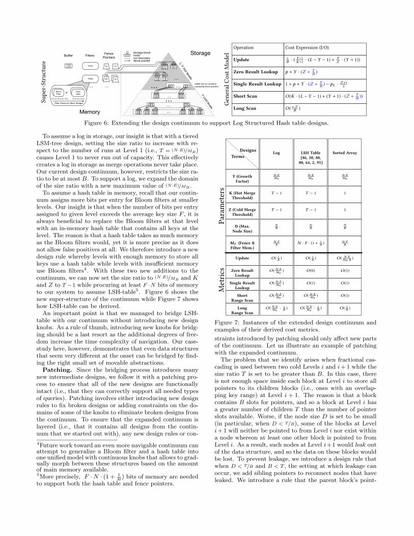
Figure 6: Extending the design continuum to support Log Structured Hash table designs.

To assume a log in storage, our insight is that with a tieredLSM-tree design, setting the size ratio to increase with re-spect to the number of runs at Level 1 (i.e., T = (N·E)/MB)causes Level 1 to never run out of capacity. This effectivelycreates a log in storage as merge operations never take place.Our current design continuum, however, restricts the size ra-tio to be at most B. To support a log, we expand the domainof the size ratio with a new maximum value of (N·E)/MB.

To assume a hash table in memory, recall that our contin-uum assigns more bits per entry for Bloom filters at smallerlevels. Our insight is that when the number of bits per entryassigned to given level exceeds the average key size F , it isalways beneficial to replace the Bloom filters at that levelwith an in-memory hash table that contains all keys at thelevel. The reason is that a hash table takes as much memoryas the Bloom filters would, yet it is more precise as it doesnot allow false positives at all. We therefore introduce a newdesign rule whereby levels with enough memory to store allkeys use a hash table while levels with insufficient memoryuse Bloom filters4. With these two new additions to thecontinuum, we can now set the size ratio to (N·E)/MB and Kand Z to T −1 while procuring at least F ·N bits of memoryto our system to assume LSH-table5. Figure 6 shows thenew super-structure of the continuum while Figure 7 showshow LSH-table can be derived.

An important point is that we managed to bridge LSH-table with our continuum without introducing new designknobs. As a rule of thumb, introducing new knobs for bridg-ing should be a last resort as the additional degrees of free-dom increase the time complexity of navigation. Our case-study here, however, demonstrates that even data structuresthat seem very different at the onset can be bridged by find-ing the right small set of movable abstractions.

Patching. Since the bridging process introduces manynew intermediate designs, we follow it with a patching pro-cess to ensure that all of the new designs are functionallyintact (i.e., that they can correctly support all needed typesof queries). Patching involves either introducing new designrules to fix broken designs or adding constraints on the do-mains of some of the knobs to eliminate broken designs fromthe continuum. To ensure that the expanded continuum islayered (i.e., that it contains all designs from the contin-uum that we started out with), any new design rules or con-

4Future work toward an even more navigable continuum canattempt to generalize a Bloom filter and a hash table intoone unified model with continuous knobs that allows to grad-ually morph between these structures based on the amountof main memory available.5More precisely, F ·N · (1 + 1

B) bits of memory are needed

to support both the hash table and fence pointers.

Para

met

ers

Met

rics

TermsDesigns Log LSH Table

[86, 20, 88,80, 64, 2, 95]

Sorted Array

T (GrowthFactor)

N ·EMB

N ·EMB

N ·EMB

K (Hot MergeThreshold)

T � 1 T � 1 1

Z (Cold MergeThreshold)

T � 1 T � 1 1

D (Max.Node Size)

NB

NB

NB

MF (Fence &Filter Mem.)

N ·FB N · F · (1 + 1

B ) N ·FB

Update O ( 1B ) O ( 1

B ) O ( N ·EMB ·B )

Zero ResultLookup

O ( N ·EMB

) O (0) O (1)

Single ResultLookup

O ( N ·EMB

) O (1) O (1)

ShortRange Scan

O ( N ·EMB

) O ( N ·EMB

) O (1)

LongRange Scan

O ( N ·EMB

· sB ) O ( N ·E

MB· s

B ) O ( sB )

Figure 7: Instances of the extended design continuum andexamples of their derived cost metrics.

straints introduced by patching should only affect new partsof the continuum. Let us illustrate an example of patchingwith the expanded continuum.

The problem that we identify arises when fractional cas-cading is used between two cold Levels i and i+ 1 while thesize ratio T is set to be greater than B. In this case, thereis not enough space inside each block at Level i to store allpointers to its children blocks (i.e., ones with an overlap-ping key range) at Level i + 1. The reason is that a blockcontains B slots for pointers, and so a block at Level i hasa greater number of children T than the number of pointerslots available. Worse, if the node size D is set to be small(in particular, when D < T/B), some of the blocks at Leveli+ 1 will neither be pointed to from Level i nor exist withina node whereon at least one other block is pointed to fromLevel i. As a result, such nodes at Level i+1 would leak outof the data structure, and so the data on these blocks wouldbe lost. To prevent leakage, we introduce a design rule thatwhen D < T/B and B < T , the setting at which leakage canoccur, we add sibling pointers to reconnect nodes that haveleaked. We introduce a rule that the parent block’s point-

ers are spatially evenly distributed across its children (every(T/(B·D))th node at Level i+ 1 is pointed to from a block atlevel i) to ensure that all sibling chains of nodes within Leveli+ 1 have an equal length. As these new rules only apply tonew parts of our continuum (i.e., when T > B), they do notviolate layering.

Costing. The final step is to generalize the continuum’scost model to account for all new designs. This requireseither extending the cost equations and/or proving that theexisting equations still hold for the new designs. Let usillustrate two examples. First, we extend the cost modelwith respect to the patch introduced above. In particular,the lookup costs need to account for having to traverse achain of sibling nodes at each of the cold levels when T > B.As the length of each chain is T/B blocks, we extend thecost equations for point lookups and short-range lookupswith additional T/B I/Os per each of the Y cold levels. Theextended cost equations are shown in Figure 6.

In the derivation below, we start with general cost ex-pression for point lookups in Figure 6 and show how theexpected point lookup cost for LSH-table is indeed derivedcorrectly. In Step 2, we plug in N/B for T and Z to assume alog in storage. In Step 3, we set the number of cold levels tozero as Level 1 in our continuum by construction is alwayshot and in this case, there is only one level (i.e., L = 1), andthus Y must be zero. In Step 4, we plug in the key size F forthe number of bits per entry for the Bloom filters, since withLSH-table there is enough space to store all keys in memory.In Step 5, we reason that the key size F must comprise onaverage at least log(N) bits to represent all unique keys. InStep 6, we simplify and omit small constants to arrive at acost of O(1) I/O per point lookup.

∈ O(1 + Z · e−(MBF/N)·TY+ Y · (Z + T/B))

∈ O(1 + N/B · e−(MBF/N)·(N/B)Y+ Y · (N/B + N/B2)) (2)

∈ O(1 + N/B · e−(MBF/N)) (3)

∈ O(1 + N/B · e−F) (4)

∈ O(1 + N/B · e− log2(N)) (5)

∈ O(1) (6)

2.5 Elegance Vs. Performance:To Expand or Not to Expand?

As new data structures continue to get invented and opti-mized, the question arises of when it is desirable to expand adesign continuum to include a new design. We show throughan example that the answer is not always clear cut.

In an effort to make B-trees more write-optimized for flashdevices, several recent B-tree designs buffer updates in mem-ory and later flush them to a log in storage in their arrivalorder. They further use an in-memory indirection table tomap each logical B-tree node to the locations in the log thatcontain entries belonging to that given node. This designcan improve on update cost relative to a regular B-tree byflushing multiple updates that target potentially differentnodes with a single sequential write. The trade-off is thatduring reads, multiple I/Os need to be issued to the logfor every logical B-tree node that gets traversed in order tofetch its contents. To bound the number of I/Os to the log,a compaction process takes place once a logical node spansover C blocks in the log, where C is a tunable parameter.

0

5

10

15

20

25

30

35

40

45

read

s(I/O

)

0.0 0.5 1.0 1.5 2.0

write cost (amortized weighted I/O)

LSB-tree (point & short range reads)Leveled LSM-tree short range readsLeveled LSM-tree point reads

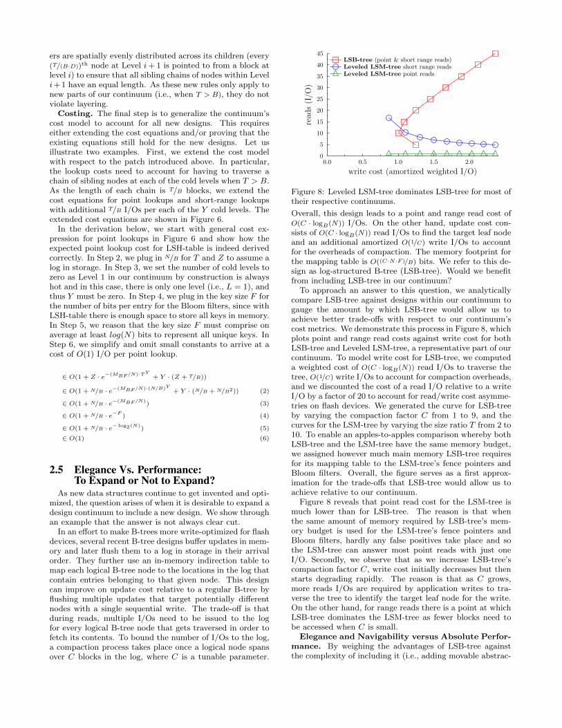
Figure 8: Leveled LSM-tree dominates LSB-tree for most oftheir respective continuums.

Overall, this design leads to a point and range read cost ofO(C · logB(N)) I/Os. On the other hand, update cost con-sists of O(C · logB(N)) read I/Os to find the target leaf nodeand an additional amortized O(1/C) write I/Os to accountfor the overheads of compaction. The memory footprint forthe mapping table is O((C·N·F )/B) bits. We refer to this de-sign as log-structured B-tree (LSB-tree). Would we benefitfrom including LSB-tree in our continuum?

To approach an answer to this question, we analyticallycompare LSB-tree against designs within our continuum togauge the amount by which LSB-tree would allow us toachieve better trade-offs with respect to our continuum’scost metrics. We demonstrate this process in Figure 8, whichplots point and range read costs against write cost for bothLSB-tree and Leveled LSM-tree, a representative part of ourcontinuum. To model write cost for LSB-tree, we computeda weighted cost of O(C · logB(N)) read I/Os to traverse thetree, O(1/C) write I/Os to account for compaction overheads,and we discounted the cost of a read I/O relative to a writeI/O by a factor of 20 to account for read/write cost asymme-tries on flash devices. We generated the curve for LSB-treeby varying the compaction factor C from 1 to 9, and thecurves for the LSM-tree by varying the size ratio T from 2 to10. To enable an apples-to-apples comparison whereby bothLSB-tree and the LSM-tree have the same memory budget,we assigned however much main memory LSB-tree requiresfor its mapping table to the LSM-tree’s fence pointers andBloom filters. Overall, the figure serves as a first approx-imation for the trade-offs that LSB-tree would allow us toachieve relative to our continuum.

Figure 8 reveals that point read cost for the LSM-tree ismuch lower than for LSB-tree. The reason is that whenthe same amount of memory required by LSB-tree’s mem-ory budget is used for the LSM-tree’s fence pointers andBloom filters, hardly any false positives take place and sothe LSM-tree can answer most point reads with just oneI/O. Secondly, we observe that as we increase LSB-tree’scompaction factor C, write cost initially decreases but thenstarts degrading rapidly. The reason is that as C grows,more reads I/Os are required by application writes to tra-verse the tree to identify the target leaf node for the write.On the other hand, for range reads there is a point at whichLSB-tree dominates the LSM-tree as fewer blocks need tobe accessed when C is small.

Elegance and Navigability versus Absolute Perfor-mance. By weighing the advantages of LSB-tree againstthe complexity of including it (i.e., adding movable abstrac-

tions to assume indirection and node compactions), one candecide to leave LSB-tree out of the continuum. This is be-cause its design principles are fundamentally different thanwhat we had included and so substantial changes would beneeded that would complicate the continuum’s constructionand navigability. On the other hand, when we did the expan-sion for LSH-table, even though, it seemed initially that thiswas a fundamentally different design, this was not the case:LSH-table is synthesized from the same design principles wealready had in the continuum, and so we could achieve theexpansion in an elegant way at no extra complexity and witha net benefit of including the new performance trade-offs.

At the other extreme, one may decide to include LSB-treebecause the additional performance trade-offs outweigh thecomplexity for a given set of desired applications. We didthis analysis to make the point of elegance and navigabil-ity versus absolute performance. However, we considered alimited set of performance metrics, i.e., worst-case I/O per-formance for writes, point reads and range reads. Most ofthe work on LSB-tree-like design has been in the contextof enabling better concurrency control [62] and leveragingworkload skew to reduce compaction frequency and over-heads [96]. Future expansion of the design space and contin-uums should include such metrics and these considerationsdescribed above for the specific example will be different. Inthis way, the decision of whether to expand or not to expanda continuum is a continual process, for which the outcomemay change over time as different cost metrics change intheir level of importance given target applications.

3. WHY NOT MUTUALLY EXCLUSIVEDESIGN COMPONENTS?

Many modern key-value stores are composed of mutuallyexclusive sets of swappable data layout designs to provide di-verse performance properties. For example, WiredTiger sup-ports separate B-tree and LSM-tree implementations to op-timize more for reads or writes, respectively, while RocksDBfiles support either a sorted strings layout or a hash tablelayout to optimize more for range reads or point reads, re-spectively. A valid question is how does this compare to thedesign continuum in general? And in practice how does itcompare to the vision of self-designing key-value stores?

Any exposure of data layout design knobs is similar inspirit and goals to the continuum but how it is done exactlyis the key. Mutually exclusive design components can be inpractice a tremendously useful tool to allow a single systemto be tuned for a broader range of applications than wewould have been able to do without this feature. However,it is not a general solution and leads to three fundamentalproblems.

1) Expensive Transitions. Predicting the optimal setof design components for a given application before deploy-ment is hard as the workload may not be known precisely. Asa result, components may need to be continually reshuffledduring runtime. Changing among large components duringruntime is disruptive as it often requires rewriting all data.In practice, the overheads associated with swapping compo-nents often force practitioners to commit to a suboptimaldesign from the onset for a given application scenario.

2) Sparse Mapping to Performance Properties. Aneven deeper problem is that mutually exclusive design com-ponents tend to have polar opposite performance properties

(e.g., hash table vs. sorted array). Swapping between twocomponents to optimize for one operation type (e.g. pointreads) may degrade a different cost metric (e.g. range reads)by so much that it would offset the gain in the first metricand lead to poorer performance overall. In other words,optimizing by shuffling components carries a risk of over-shooting the target performance properties and hitting thepoint of diminishing returns. A useful way of thinking aboutthis problem is that mutually exclusive design componentsmap sparsely onto the space of possible performance proper-ties. The problem is that, with large components, there areno intermediate designs that allow to navigate performanceproperties in smaller steps.

3) Intractable Modeling. Even analytically, it quicklybecomes intractable to reason about the tens to hundredsof tuning parameters in modern key-value stores and howthey interact with all the different mutually exclusive designcomponents to lead to different performance properties. Anentirely new performance model is often needed for eachpermutation of design components, and that the number ofpossible permutations increases exponentially with respectto the number of components available. Creating such anextensive set of models and trying to optimize across themquickly becomes intractable. This problem gets worse assystems mature and more components get added and it boilsdown to manual tuning by experts.

The Design Continuum Spirit. Our work helps withthis problem by formalizing this data layout design spaceso that educated decisions can be made easily and quickly,sometimes even automatically. Design continuums deal witheven more knobs than what existing systems expose becausethey try to capture the fundamental design principles of de-sign which by definition are more fine-grained concepts. Forexample, a sorted array is already a full data structure thatcan be synthesized out of many smaller decisions. However,the key is that design continuums know how to navigatethose fine-grained concepts and eventually expose to design-ers a much smaller set of knobs and a way to argue directly atthe performance tradeoff level. The key lies in constructingdesign continuums and key-value store systems via unifiedmodels and implementations with continuous data layoutdesign knobs rather than swappable components.

For example, the advantage of supporting LSH-table bycontinuum expansion rather than as an independent swap-pable component is that the bridging process adds new in-termediate designs into the continuum with appealing trade-offs in-between. The new continuum allows us to graduallytransition from a tiered LSM-tree into LSH-table by increas-ing the size ratio in small increments to optimize more forwrites at the expense of range reads and avoid overshootingthe optimal performance properties when tuning.

4. ENHANCING CREATIVITYBeyond the ability to assume existing designs, a contin-

uum can also assist in identifying new data structure designsthat were unknown before, but they are naturally derivedfrom the continuum’s design parameters and rules.

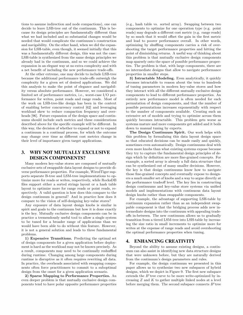
For example, the design continuum we presented in thispaper allows us to synthesize two new subspaces of hybriddesigns, which we depict in Figure 9. The first new subspaceextends the Bεtree curve to be more write-optimized by in-creasing Z and K to gather multiple linked nodes at a levelbefore merging them. The second subspace connects Bεtree

update cost (I/O)

O 1𝐵 ∙log2

𝑁𝐵∙𝐷 O log𝐵

𝑁𝐵∙𝐷

single

res

ult lookup c

ost

(I/

O)

O 1

O 1

O log2𝑁𝐵∙𝐷

O log𝐵𝑁𝐵∙𝐷

B+-tree

Be-tree with 𝑀𝐹 = 0LSM-tree with 𝑀𝐹 = 𝑁 ∙ (𝐹𝐵 + 10)

new designs

O 𝐵∙log𝐵𝑁𝐵∙𝐷

O 1+𝐵∙𝑒2𝑀𝐵𝐹/𝑁

O 1𝐵 ∙log𝐵

𝑁𝐵∙𝐷

Figure 9: Visualizing the performance continuum.

with LSM-tree designs, allowing first to optimize for writesand lookups at hot levels by using Bloom filters and fencepointers, and second to minimize memory investment at coldlevels by using fractional cascading instead. Thus, we turnthe design space into a multi-dimensional space whereon ev-ery point maps onto a unique position along a hyperplane ofPareto-optimal performance trade-offs (as opposed to hav-ing to choose between drastically different designs only).

In addition, as the knobs in a bijective continuum are di-mensions that interact to yield unique designs, expandingany knob’s domain or adding new knobs during the bridg-ing process can in fact enrich a continuum with new, gooddesigns that were not a part of the original motivation forexpansion. Such examples are present in our expanded con-tinuum where our original goal was to include LSH-table.For example, fixing K and Z to 1 and increasing the sizeratio beyond B towards N/(D·P ) allows us to gradually tran-sition from a leveled LSM-tree into a sorted array (as even-tually there is only one level). This design was not possiblebefore, and it is beneficial for workloads with many rangereads. In this way, the bridging process makes a continuumincreasingly rich and powerful.

What is a new Data Structure? There are a numberof open questions this work touches on. And some of thesequestions become even philosophical. For example, if alldata structures can be described as combinations of a smallset of design principles, then what constitutes a new datastructure design? Given the vastness of the design space, wethink that the discovery of any combination of design princi-ples that brings new and interesting performance propertiesclassifies as a new data structure. Historically, this has beenthe factor of recognizing new designs as worthy and inter-esting even if seemingly “small” differences separated them.For example, while an LSM-tree can simply be seen as asequence of unmerged B-trees, the performance propertiesit brings are so drastically different that it has become itsown category of study and whole systems are built aroundits basic design principles.

5. THE PATH TO SELF-DESIGNKnowing which design is the best for a workload opens

the opportunity for systems that can adapt on-the-fly. Whileadaptivity has been studied in several forms including adapt-ing storage to queries [41, 4, 12, 49, 43, 30, 40, 66], thenew opportunity is morphing among what is typically con-sidered as fundamentally different designs, e.g., from an

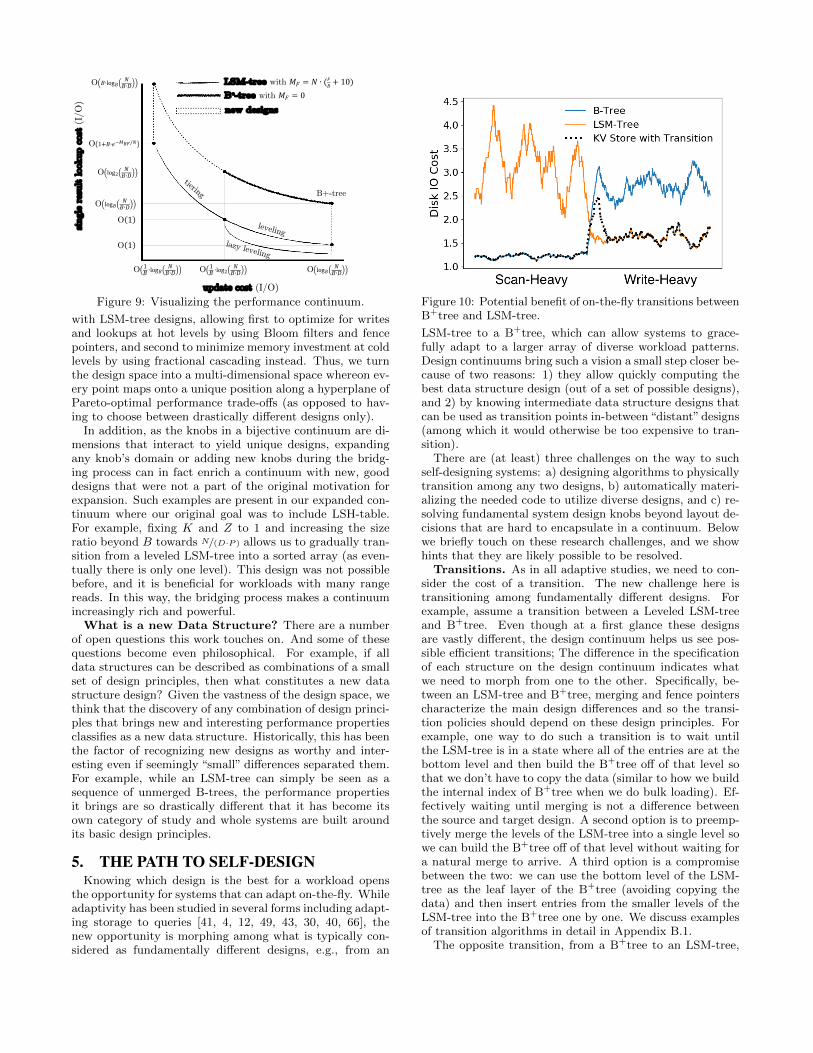
Figure 10: Potential benefit of on-the-fly transitions betweenB+tree and LSM-tree.

LSM-tree to a B+tree, which can allow systems to grace-fully adapt to a larger array of diverse workload patterns.Design continuums bring such a vision a small step closer be-cause of two reasons: 1) they allow quickly computing thebest data structure design (out of a set of possible designs),and 2) by knowing intermediate data structure designs thatcan be used as transition points in-between “distant” designs(among which it would otherwise be too expensive to tran-sition).

There are (at least) three challenges on the way to suchself-designing systems: a) designing algorithms to physicallytransition among any two designs, b) automatically materi-alizing the needed code to utilize diverse designs, and c) re-solving fundamental system design knobs beyond layout de-cisions that are hard to encapsulate in a continuum. Belowwe briefly touch on these research challenges, and we showhints that they are likely possible to be resolved.

Transitions. As in all adaptive studies, we need to con-sider the cost of a transition. The new challenge here istransitioning among fundamentally different designs. Forexample, assume a transition between a Leveled LSM-treeand B+tree. Even though at a first glance these designsare vastly different, the design continuum helps us see pos-sible efficient transitions; The difference in the specificationof each structure on the design continuum indicates whatwe need to morph from one to the other. Specifically, be-tween an LSM-tree and B+tree, merging and fence pointerscharacterize the main design differences and so the transi-tion policies should depend on these design principles. Forexample, one way to do such a transition is to wait untilthe LSM-tree is in a state where all of the entries are at thebottom level and then build the B+tree off of that level sothat we don’t have to copy the data (similar to how we buildthe internal index of B+tree when we do bulk loading). Ef-fectively waiting until merging is not a difference betweenthe source and target design. A second option is to preemp-tively merge the levels of the LSM-tree into a single level sowe can build the B+tree off of that level without waiting fora natural merge to arrive. A third option is a compromisebetween the two: we can use the bottom level of the LSM-tree as the leaf layer of the B+tree (avoiding copying thedata) and then insert entries from the smaller levels of theLSM-tree into the B+tree one by one. We discuss examplesof transition algorithms in detail in Appendix B.1.

The opposite transition, from a B+tree to an LSM-tree,

1 PointLookup (searchKey)2 if MB > E then3 entry := buffer.find(searchKey);4 if entry then5 return entry ;

// Pointer for direct block access. Set to root.6 blockToCheck := levels[0].runs[0].nodes[0];7 for i← 0 to L do

// Check each level’s runs from recent to oldest.8 for j ← 0 to levels[i].runs.count do

/* Prune search using bloom filters and fenceswhen available. */

9 if i < (L− Y ) // At hot levels.10 then11 keyCouldExist :=

filters[i][j].checkExists(searchKey);12 if !keyCouldExist then13 continue;14 else15 blockToCheck :=

fences[i][j].find(searchKey);

/* For oldest hot run, and all cold runs, if noentry is returned, then the search continuesusing a pointer into the next oldest run. */

16 entry, blockToCheck :=blockToCheck.find(searchKey);

17 if entry then18 return entry;

19 return keyDoesNotExist;

Algorithm 1: Lookup algorithm template for any design.

is also possible with the reverse problem that the scatteredleaves of the B+tree need to represent a contiguous run in anLSM-tree. To avoid a full write we can trick virtual memoryto see these pages as contiguous [83]. The very first timethe new LSM-tree does a full merge, the state goes back tophysically contiguous runs. We explore the implementation-level concerns of keeping the data layouts of such designsinteroperable in Appendix B.2.

Figure 10 depicts the potential of transitions. During thefirst 2000 queries, the workload is short-range scan heavyand thus favors B+tree. During the next 2000 queries, theworkload becomes write heavy, favoring LSM-Trees. Whilepure LSM-tree and pure B-tree designs fail to achieve glob-ally good performance, when using transitions, we can stayclose to the optimal performance across the whole workload.The figure captures the I/O behavior of these data structuredesigns and the transitions (in number of blocks). Overall,it is possible to do transitions at a smaller cost than readingand writing all data even if we transition among fundamen-tally different structures. The future path for the realizationof this vision points to a transition algebra.

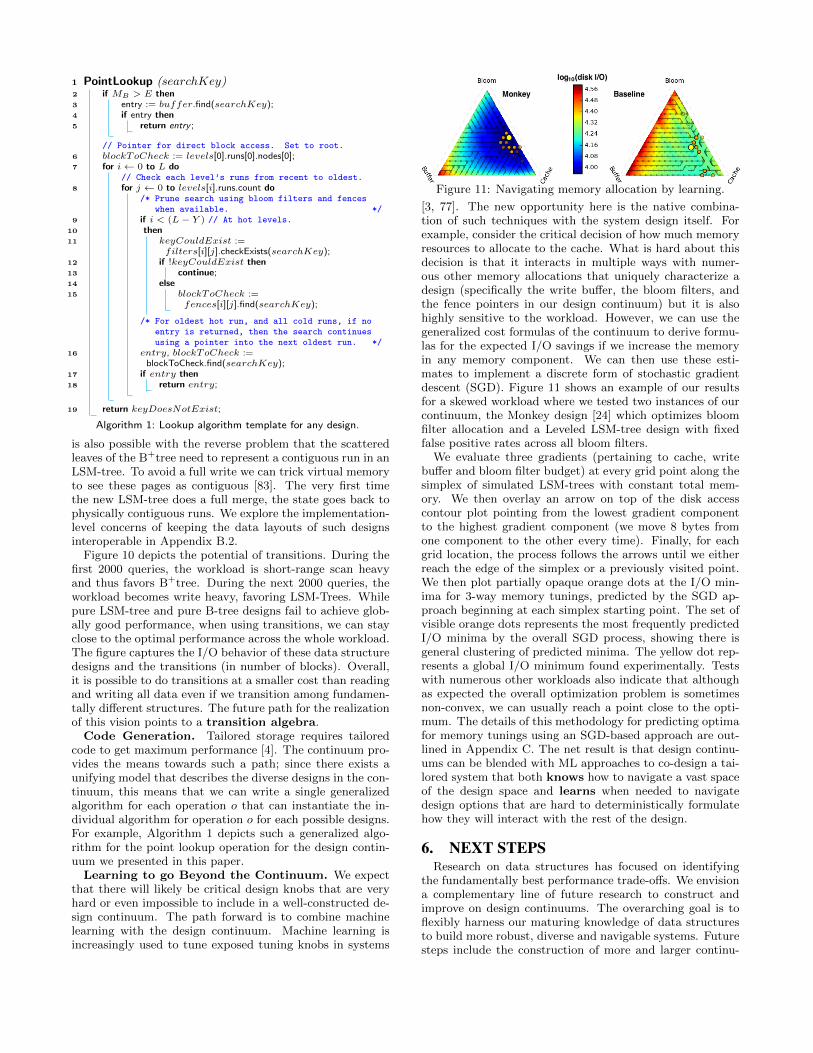
Code Generation. Tailored storage requires tailoredcode to get maximum performance [4]. The continuum pro-vides the means towards such a path; since there exists aunifying model that describes the diverse designs in the con-tinuum, this means that we can write a single generalizedalgorithm for each operation o that can instantiate the in-dividual algorithm for operation o for each possible designs.For example, Algorithm 1 depicts such a generalized algo-rithm for the point lookup operation for the design contin-uum we presented in this paper.

Learning to go Beyond the Continuum. We expectthat there will likely be critical design knobs that are veryhard or even impossible to include in a well-constructed de-sign continuum. The path forward is to combine machinelearning with the design continuum. Machine learning isincreasingly used to tune exposed tuning knobs in systems

Figure 11: Navigating memory allocation by learning.

[3, 77]. The new opportunity here is the native combina-tion of such techniques with the system design itself. Forexample, consider the critical decision of how much memoryresources to allocate to the cache. What is hard about thisdecision is that it interacts in multiple ways with numer-ous other memory allocations that uniquely characterize adesign (specifically the write buffer, the bloom filters, andthe fence pointers in our design continuum) but it is alsohighly sensitive to the workload. However, we can use thegeneralized cost formulas of the continuum to derive formu-las for the expected I/O savings if we increase the memoryin any memory component. We can then use these esti-mates to implement a discrete form of stochastic gradientdescent (SGD). Figure 11 shows an example of our resultsfor a skewed workload where we tested two instances of ourcontinuum, the Monkey design [24] which optimizes bloomfilter allocation and a Leveled LSM-tree design with fixedfalse positive rates across all bloom filters.

We evaluate three gradients (pertaining to cache, writebuffer and bloom filter budget) at every grid point along thesimplex of simulated LSM-trees with constant total mem-ory. We then overlay an arrow on top of the disk accesscontour plot pointing from the lowest gradient componentto the highest gradient component (we move 8 bytes fromone component to the other every time). Finally, for eachgrid location, the process follows the arrows until we eitherreach the edge of the simplex or a previously visited point.We then plot partially opaque orange dots at the I/O min-ima for 3-way memory tunings, predicted by the SGD ap-proach beginning at each simplex starting point. The set ofvisible orange dots represents the most frequently predictedI/O minima by the overall SGD process, showing there isgeneral clustering of predicted minima. The yellow dot rep-resents a global I/O minimum found experimentally. Testswith numerous other workloads also indicate that althoughas expected the overall optimization problem is sometimesnon-convex, we can usually reach a point close to the opti-mum. The details of this methodology for predicting optimafor memory tunings using an SGD-based approach are out-lined in Appendix C. The net result is that design continu-ums can be blended with ML approaches to co-design a tai-lored system that both knows how to navigate a vast spaceof the design space and learns when needed to navigatedesign options that are hard to deterministically formulatehow they will interact with the rest of the design.

6. NEXT STEPSResearch on data structures has focused on identifying

the fundamentally best performance trade-offs. We envisiona complementary line of future research to construct andimprove on design continuums. The overarching goal is toflexibly harness our maturing knowledge of data structuresto build more robust, diverse and navigable systems. Futuresteps include the construction of more and larger continu-

ums, and especially the investigation of broader classes ofdata structure design, including graphs, spatial data, com-pression, replication as well as crucially more performancemetrics such as concurrency, and adaptivity. The most chal-lenging next step is whether the construction of design con-tinuums itself can be (semi-) automated.

7. ACKNOWLEDGMENTSMark Callaghan has provided the authors with feedback

and insights on key-value store design and industry prac-tices repeatedly over the past few years and specifically forthis paper. This work is supported by the National ScienceFoundation under grant IIS-1452595.

8. REFERENCES[1] N. Agrawal, V. Prabhakaran, T. Wobber, J. D. Davis, M. Manasse,

and R. Panigrahy. Design Tradeoffs for SSD Performance. ATC,2008.

[2] J.-S. Ahn, C. Seo, R. Mayuram, R. Yaseen, J.-S. Kim, andS. Maeng. ForestDB: A Fast Key-Value Storage System forVariable-Length String Keys. TC, 65(3):902–915, 2016.

[3] D. V. Aken, A. Pavlo, G. J. Gordon, and B. Zhang. AutomaticDatabase Management System Tuning Through Large-scale MachineLearning. SIGMOD, 2017.

[4] I. Alagiannis, S. Idreos, and A. Ailamaki. H2O: A Hands-freeAdaptive Store. SIGMOD, 2014.

[5] D. J. Aldous. Exchangeability and related topics. pages 1–198, 1985.

[6] P. M. Aoki. Generalizing ”Search” in Generalized Search Trees(Extended Abstract). ICDE, 1998.

[7] P. M. Aoki. How to Avoid Building DataBlades That Know theValue of Everything and the Cost of Nothing. SSDBM, 1999.

[8] Apache. Accumulo. https://accumulo.apache.org/.

[9] Apple. Foundationdb. https://github.com/apple/foundationdb, 2018.

[10] L. Arge. The Buffer Tree: A Technique for Designing BatchedExternal Data Structures. Algorithmica, 37(1):1–24, 2003.

[11] T. G. Armstrong, V. Ponnekanti, D. Borthakur, and M. Callaghan.LinkBench: a Database Benchmark Based on the Facebook SocialGraph. SIGMOD, 2013.

[12] J. Arulraj, A. Pavlo, and P. Menon. Bridging the Archipelagobetween Row-Stores and Column-Stores for Hybrid Workloads.SIGMOD, 2016.

[13] M. Athanassoulis, M. S. Kester, L. M. Maas, R. Stoica, S. Idreos,A. Ailamaki, and M. Callaghan. Designing Access Methods: TheRUM Conjecture. EDBT, 2016.

[14] R. Bayer and E. M. McCreight. Organization and Maintenance ofLarge Ordered Indexes. Proceedings of the ACM SIGFIDETWorkshop on Data Description and Access, 1970.

[15] R. Bayer and E. M. McCreight. Organization and Maintenance ofLarge Ordered Indices. Acta Informatica, 1(3):173–189, 1972.

[16] M. A. Bender, M. Farach-Colton, J. T. Fineman, Y. R. Fogel, B. C.Kuszmaul, and J. Nelson. Cache-Oblivious Streaming B-trees.SPAA, 2007.

[17] G. S. Brodal and R. Fagerberg. Lower Bounds for External MemoryDictionaries. SODA, 2003.

[18] Y. Bu, V. R. Borkar, J. Jia, M. J. Carey, and T. Condie. Pregelix:Big(ger) Graph Analytics on a Dataflow Engine. PVLDB,8(2):161–172, 2014.

[19] Z. Cao, S. Chen, F. Li, M. Wang, and X. S. Wang. LogKV:Exploiting Key-Value Stores for Log Processing. CIDR, 2013.

[20] B. Chandramouli, G. Prasaad, D. Kossmann, J. J. Levandoski,J. Hunter, and M. Barnett. FASTER: A Concurrent Key-Value Storewith In-Place Updates. SIGMOD, 2018.

[21] F. Chang, J. Dean, S. Ghemawat, W. C. Hsieh, D. A. Wallach,M. Burrows, T. Chandra, A. Fikes, and R. E. Gruber. Bigtable: ADistributed Storage System for Structured Data. OSDI, 2006.

[22] D. Cohen and N. Campbell. Automating Relational Operations onData Structures. IEEE Software, 10(3):53–60, 1993.

[23] B. Dageville, T. Cruanes, M. Zukowski, V. Antonov, A. Avanes,J. Bock, J. Claybaugh, D. Engovatov, M. Hentschel, J. Huang,A. W. Lee, A. Motivala, A. Q. Munir, S. Pelley, P. Povinec,G. Rahn, S. Triantafyllis, and P. Unterbrunner. The SnowflakeElastic Data Warehouse. SIGMOD, 2016.

[24] N. Dayan, M. Athanassoulis, and S. Idreos. Monkey: OptimalNavigable Key-Value Store. SIGMOD, 2017.

[25] N. Dayan, M. Athanassoulis, and S. Idreos. Optimal Bloom Filtersand Adaptive Merging for LSM-Trees. TODS, (to appear, 2018.

[26] N. Dayan, P. Bonnet, and S. Idreos. GeckoFTL: Scalable FlashTranslation Techniques For Very Large Flash Devices. SIGMOD,2016.

[27] N. Dayan and S. Idreos. Dostoevsky: Better Space-Time Trade-Offsfor LSM-Tree Based Key-Value Stores via Adaptive Removal ofSuperfluous Merging. SIGMOD, 2018.

[28] N. Dayan and S. Idreos. The log-structured merge-bush & the wackycontinuum. In SIGMOD, 2019.

[29] G. DeCandia, D. Hastorun, M. Jampani, G. Kakulapati,A. Lakshman, A. Pilchin, S. Sivasubramanian, P. Vosshall, andW. Vogels. Dynamo: Amazon’s Highly Available Key-value Store.SIGOPS Op. Sys. Rev., 41(6):205–220, 2007.

[30] J. Dittrich and A. Jindal. Towards a One Size Fits All DatabaseArchitecture. CIDR, 2011.

[31] S. Dong, M. Callaghan, L. Galanis, D. Borthakur, T. Savor, andM. Strum. Optimizing Space Amplification in RocksDB. CIDR, 2017.

[32] Facebook. RocksDB. https://github.com/facebook/rocksdb.

[33] M. J. Franklin. Caching and Memory Management in Client-ServerDatabase Systems. PhD thesis, University of Wisconsin-Madison,1993.

[34] G. Golan-Gueta, E. Bortnikov, E. Hillel, and I. Keidar. ScalingConcurrent Log-Structured Data Stores. EuroSys, 2015.

[35] Google. LevelDB. https://github.com/google/leveldb/.

[36] P. Hawkins, A. Aiken, K. Fisher, M. C. Rinard, and M. Sagiv. DataRepresentation Synthesis. PLDI, 2011.

[37] P. Hawkins, A. Aiken, K. Fisher, M. C. Rinard, and M. Sagiv.Concurrent data representation synthesis. PLDI, 2012.

[38] HBase. Online reference. http://hbase.apache.org/, 2013.

[39] J. M. Hellerstein, J. F. Naughton, and A. Pfeffer. GeneralizedSearch Trees for Database Systems. VLDB, 1995.

[40] S. Idreos, I. Alagiannis, R. Johnson, and A. Ailamaki. Here are myData Files. Here are my Queries. Where are my Results? CIDR,2011.

[41] S. Idreos, M. L. Kersten, and S. Manegold. Database Cracking.CIDR, 2007.

[42] S. Idreos, L. M. Maas, and M. S. Kester. Evolutionary DataSystems. CoRR, abs/1706.0, 2017.

[43] S. Idreos, S. Manegold, H. Kuno, and G. Graefe. Merging What’sCracked, Cracking What’s Merged: Adaptive Indexing inMain-Memory Column-Stores. PVLDB, 4(9):586–597, 2011.

[44] S. Idreos, K. Zoumpatianos, M. Athanassoulis, N. Dayan,B. Hentschel, M. S. Kester, D. Guo, L. M. Maas, W. Qin, A. Wasay,and Y. Sun. The Periodic Table of Data Structures. IEEE DEBULL,41(3):64–75, 2018.

[45] S. Idreos, K. Zoumpatianos, B. Hentschel, M. S. Kester, and D. Guo.The Data Calculator: Data Structure Design and Cost Synthesisfrom First Principles and Learned Cost Models. SIGMOD, 2018.

[46] H. V. Jagadish, P. P. S. Narayan, S. Seshadri, S. Sudarshan, andR. Kanneganti. Incremental Organization for Data Recording andWarehousing. VLDB, 1997.

[47] W. Jannen, J. Yuan, Y. Zhan, A. Akshintala, J. Esmet, Y. Jiao,A. Mittal, P. Pandey, P. Reddy, L. Walsh, M. A. Bender,M. Farach-Colton, R. Johnson, B. C. Kuszmaul, and D. E. Porter.BetrFS: A Right-optimized Write-optimized File System. FAST,2015.

[48] C. Jermaine, E. Omiecinski, and W. G. Yee. The PartitionedExponential File for Database Storage Management. VLDBJ,16(4):417–437, 2007.

[49] O. Kennedy and L. Ziarek. Just-In-Time Data Structures. CIDR,2015.

[50] M. L. Kersten and L. Sidirourgos. A database system with amnesia.In CIDR, 2017.

[51] H. Kondylakis, N. Dayan, K. Zoumpatianos, and T. Palpanas.Coconut: A scalable bottom-up approach for building data seriesindexes. VLDB, 11(6):677–690, 2018.

[52] H. Kondylakis, N. Dayan, K. Zoumpatianos, and T. Palpanas.Coconut palm: Static and streaming data series exploration now inyour palm. In SIGMOD, 2019.

[53] M. Kornacker. High-Performance Extensible Indexing. VLDB, 1999.

[54] M. Kornacker, C. Mohan, and J. M. Hellerstein. Concurrency andRecovery in Generalized Search Trees. SIGMOD, 1997.

[55] M. Kornacker, M. A. Shah, and J. M. Hellerstein. amdb: An AccessMethod Debugging Tool. SIGMOD, 1998.

[56] M. Kornacker, M. A. Shah, and J. M. Hellerstein. Amdb: A DesignTool for Access Methods. IEEE DEBULL, 26(2):3–11, 2003.

[57] D. Kossman. Systems Research - Fueling Future Disruptions. InKeynote talk at the Microsoft Research Faculty Summit, Redmond,WA, USA, aug 2018.

[58] T. Kraska, M. Alizadeh, A. Beutel, E. Chi, A. Kristo, G. Leclerc,S. Madden, H. Mao, and V. Nathan. Sagedb: A learned databasesystem. In CIDR, 2019.

[59] T. Kraska, A. Beutel, E. H. Chi, J. Dean, and N. Polyzotis. TheCase for Learned Index Structures. SIGMOD, 2018.

[60] A. Lakshman and P. Malik. Cassandra - A Decentralized StructuredStorage System. SIGOPS Op. Sys. Rev., 44(2):35–40, 2010.

[61] V. Leis, A. Kemper, and T. Neumann. The Adaptive Radix Tree:ARTful Indexing for Main-Memory Databases. ICDE, 2013.

[62] J. J. Levandoski, D. B. Lomet, and S. Sengupta. The Bw-Tree: AB-tree for New Hardware Platforms. ICDE, 2013.

[63] Y. Li, B. He, J. Yang, Q. Luo, K. Yi, and R. J. Yang. Tree Indexingon Solid State Drives. PVLDB, 3(1-2):1195–1206, 2010.

[64] H. Lim, D. Han, D. G. Andersen, and M. Kaminsky. MICA: AHolistic Approach to Fast In-Memory Key-Value Storage. NSDI,2014.

[65] LinkedIn. Voldemort. http://www.project-voldemort.com.

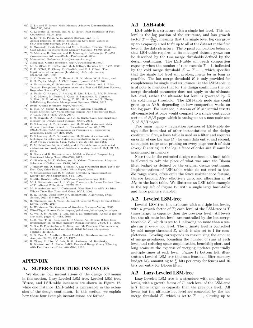
[66] Z. Liu and S. Idreos. Main Memory Adaptive Denormalization.SIGMOD, 2016.

[67] C. Loncaric, E. Torlak, and M. D. Ernst. Fast Synthesis of FastCollections. PLDI, 2016.

[68] L. Lu, T. S. Pillai, A. C. Arpaci-Dusseau, and R. H.Arpaci-Dusseau. WiscKey: Separating Keys from Values inSSD-conscious Storage. FAST, 2016.

[69] S. Manegold, P. A. Boncz, and M. L. Kersten. Generic DatabaseCost Models for Hierarchical Memory Systems. VLDB, 2002.

[70] T. Mattson, B. Sanders, and B. Massingill. Patterns for ParallelProgramming. Addison-Wesley Professional, 2004.

[71] Memcached. Reference. http://memcached.org/.

[72] MongoDB. Online reference. http://www.mongodb.com/.

[73] M. A. Olson, K. Bostic, and M. I. Seltzer. Berkeley DB. ATC, 1999.

[74] P. E. O’Neil, E. Cheng, D. Gawlick, and E. J. O’Neil. Thelog-structured merge-tree (LSM-tree). Acta Informatica,33(4):351–385, 1996.

[75] J. K. Ousterhout, G. T. Hamachi, R. N. Mayo, W. S. Scott, andG. S. Taylor. Magic: A VLSI Layout System. DAC, 1984.

[76] A. Papagiannis, G. Saloustros, P. Gonzalez-Ferez, and A. Bilas.Tucana: Design and Implementation of a Fast and Efficient Scale-upKey-value Store. ATC, 2016.

[77] A. Pavlo, G. Angulo, J. Arulraj, H. Lin, J. Lin, L. Ma, P. Menon,T. C. Mowry, M. Perron, I. Quah, S. Santurkar, A. Tomasic,S. Toor, D. V. Aken, Z. Wang, Y. Wu, R. Xian, and T. Zhang.Self-Driving Database Management Systems. CIDR, 2017.

[78] Redis. Online reference. http://redis.io/.

[79] K. Ren, Q. Zheng, J. Arulraj, and G. Gibson. SlimDB: ASpace-Efficient Key-Value Storage Engine For Semi-Sorted Data.PVLDB, 10(13):2037–2048, 2017.

[80] S. M. Rumble, A. Kejriwal, and J. K. Ousterhout. Log-structuredmemory for DRAM-based storage. FAST, 2014.

[81] E. Schonberg, J. T. Schwartz, and M. Sharir. Automatic datastructure selection in setl. In Proceedings of the 6th ACMSIGACT-SIGPLAN Symposium on Principles of ProgrammingLanguages, pages 197–210, 1979.

[82] E. Schonberg, J. T. Schwartz, and M. Sharir. An automatictechnique for selection of data representations in setl programs.ACM Trans. Program. Lang. Syst., 3(2):126–143, apr 1981.

[83] F. M. Schuhknecht, A. Jindal, and J. Dittrich. An experimentalevaluation and analysis of database cracking. VLDBJ, 25(1):27–52,2016.

[84] R. Sears and R. Ramakrishnan. bLSM: A General Purpose LogStructured Merge Tree. SIGMOD, 2012.

[85] O. Shacham, M. T. Vechev, and E. Yahav. Chameleon: AdaptiveSelection of Collections. PLDI, 2009.

[86] J. Sheehy and D. Smith. Bitcask: A Log-Structured Hash Table forFast Key/Value Data. Basho White Paper, 2010.

[87] Y. Smaragdakis and D. S. Batory. DiSTiL: A TransformationLibrary for Data Structures. DSL, 1997.

[88] Spotify. Sparkey. https://github.com/spotify/sparkey, 2014.

[89] M. J. Steindorfer and J. J. Vinju. Towards a Software Product Lineof Trie-Based Collections. GPCE, 2016.

[90] M. Stonebraker and U. Cetintemel. ”One Size Fits All”: An IdeaWhose Time Has Come and Gone. ICDE, 2005.

[91] R. E. Tarjan. Complexity of Combinatorial Algorithms. SIAMReview, 20(3):457–491, 1978.

[92] R. Thonangi and J. Yang. On Log-Structured Merge for Solid-StateDrives. ICDE, 2017.

[93] L. Wilkinson. The Grammar of Graphics. Springer-Verlag, 2005.

[94] WiredTiger. Source Code. https://github.com/wiredtiger/wiredtiger.

[95] C. Wu, J. M. Faleiro, Y. Lin, and J. M. Hellerstein. Anna: A kvs forany scale. pages 401–412, 2018.

[96] C.-H. Wu, T.-W. Kuo, and L.-P. Chang. An efficient B-tree layerimplementation for flash-memory storage systems. TECS, 6(3), 2007.

[97] Y. Xu, E. Frachtenberg, S. Jiang, and M. Paleczny. Characterizingfacebook’s memcached workload. IEEE Internet Computing,18(2):41–49, 2014.

[98] S. B. Yao. An Attribute Based Model for Database Access CostAnalysis. TODS, 2(1):45–67, 1977.

[99] H. Zhang, H. Lim, V. Leis, D. G. Andersen, M. Kaminsky,K. Keeton, and A. Pavlo. SuRF: Practical Range Query Filteringwith Fast Succinct Tries. SIGMOD, 2018.

APPENDIXA. SUPER-STRUCTURE INSTANCES

We discuss four instantiations of the design continuumin this section. Lazy-Leveled LSM-tree, Leveled LSM-tree,Bεtree, and LSH-table instances are shown in Figure 12.while one instance (LSH-table) is expressable in the exten-sion of the design continuum. In this section, we explainhow these four example instantiations are formed.

A.1 LSH-tableLSH-table is a structure with a single hot level. This hot

level is the log portion of the structure, and has growthfactor T = N·E

MB, meaning that the single level log can grow

up to a capacity sized to fit up to all of the dataset in the firstlevel of the data structure. The typical compaction behaviorthat LSH-table requires as its managed dataset grows canbe described by the two merge thresholds defined by thedesign continuum. The LSH-table will reach compactioncapacity when the number of runs exceeds T − 1, indicatedby the cold merge threshold Z = T − 1, which specifiesthat the single hot level will prolong merge for as long aspossible. The hot merge threshold K is only provided forcompleteness for single level structures like the LSH-table; itis of note to mention that for the design continuum the hotmerge threshold parameter does not apply to the ultimatehot level, rather the ultimate hot level is governed by Zthe cold merge threshold. The LSH-table node size couldgrow up to N/B, depending on how compaction works onthe log part. For instance, a stream of N sequential insertsall compacted at once would compact to a single contiguoussection of N/B pages which is analagous to a max node sizeD of N/B pages.

Two main memory navigation features of LSH-table de-sign differ from that of other instantiations of the designcontinuum: first, a hash table is used as a filter and requireson order of one key size (F ) for each data entry, and second,to support range scan pruning on every page worth of data(every B entries) in the log, a fence of order size F must bemaintained in memory.

Note that in the extended design continuum a hash tableis allowed to take the place of what was once the Bloomfilter budget as defined by the original design continuum.Implementations of LSH-table which do not need to han-dle range scans, often omit the fence maintenance feature,thereby keeping MFP effectively zero, and allocating all ofMF to the hash table. We illustrate an LSH-table examplein the top left of Figure 12; with a single large hash-tableand fence pointers enabled.

A.2 Leveled LSM-treeLeveled LSM-tree is a structure with multiple hot levels,

with a growth factor of T ; each level of the LSM-tree is Ttimes larger in capacity than the previous level. All levelsbut the ultimate hot level, are controlled by the hot mergethreshold K, which is set to 1, allowing no more than a sin-gle run at every hot level. The ultimate level is controlledby cold merge threshold Z, which is also set to 1 for com-pleteness. Leveling corresponds to maximizing the amountof merge greediness, bounding the number of runs at eachlevel, and reducing space amplification, benefiting short andlong scans at the expense of merging updates potentiallymultiple times at each level. Figure 12 bottom left, illus-trates a Leveled LSM-tree that uses fence and filter memorybudget MF amounting to F

Bbits per entry for fences and 10

bits per entry for Bloom filter.

A.3 Lazy-Leveled LSM-treeLazy-Leveled LSM-tree is a structure with multiple hot

levels, with a growth factor of T ; each level of the LSM-treeis T times larger in capacity than the previous level. Alllevels but the ultimate hot level are controlled by the hotmerge threshold K, which is set to T − 1, allowing up to

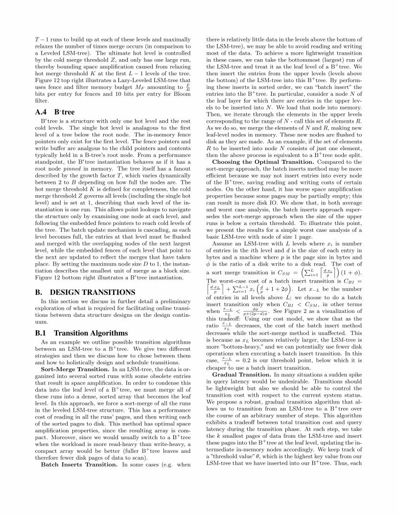
T −1 runs to build up at each of these levels and maximallyrelaxes the number of times merge occurs (in comparison toa Leveled LSM-tree). The ultimate hot level is controlledby the cold merge threshold Z, and only has one large run,thereby bounding space amplification caused from relaxinghot merge threshold K at the first L − 1 levels of the tree.Figure 12 top right illustrates a Lazy-Leveled LSM-tree thatuses fence and filter memory budget MF amounting to F

Bbits per entry for fences and 10 bits per entry for Bloomfilter.

A.4 BεtreeBεtree is a structure with only one hot level and the rest

cold levels. The single hot level is analagous to the firstlevel of a tree below the root node. The in-memory fencepointers only exist for the first level. The fence pointers andwrite buffer are analgous to the child pointers and contentstypically held in a B-tree’s root node. From a performancestandpoint, the Bεtree instantiation behaves as if it has aroot node pinned in memory. The tree itself has a fanoutdescribed by the growth factor T , which varies dynamicallybetween 2 to B depending on how full the nodes are. Thehot merge threshold K is defined for completeness, the coldmerge threshold Z governs all levels (including the single hotlevel) and is set at 1, describing that each level of the in-stantiation is one run. This allows point lookups to navigatethe structure only by examining one node at each level, andfollowing the embedded fence pointers to reach cold levels ofthe tree. The batch update mechanism is cascading, as eachlevel becomes full, the entries at that level must be flushedand merged with the overlapping nodes of the next largestlevel, while the embedded fences of each level that point tothe next are updated to reflect the merges that have takenplace. By setting the maximum node size D to 1, the instan-tiation describes the smallest unit of merge as a block size.Figure 12 bottom right illustrates a Bεtree instantiation.

B. DESIGN TRANSITIONSIn this section we discuss in further detail a preliminary

exploration of what is required for facilitating online transi-tions between data structure designs on the design contin-uum.

B.1 Transition AlgorithmsAs an example we outline possible transition algorithms

between an LSM-tree to a B+tree. We give two differentstrategies and then we discuss how to chose between themand how to holistically design and schedule transitions.

Sort-Merge Transition. In an LSM-tree, the data is or-ganized into several sorted runs with some obsolete entriesthat result in space amplification. In order to condense thisdata into the leaf level of a B+tree, we must merge all ofthese runs into a dense, sorted array that becomes the leaflevel. In this approach, we force a sort-merge of all the runsin the leveled LSM-tree structure. This has a performancecost of reading in all the runs’ pages, and then writing eachof the sorted pages to disk. This method has optimal spaceamplification properties, since the resulting array is com-pact. Moreover, since we would usually switch to a B+treewhen the workload is more read-heavy than write-heavy, acompact array would be better (fuller B+tree leaves andtherefore fewer disk pages of data to scan).

Batch Inserts Transition. In some cases (e.g. when

there is relatively little data in the levels above the bottom ofthe LSM-tree), we may be able to avoid reading and writingmost of the data. To achieve a more lightweight transitionin these cases, we can take the bottommost (largest) run ofthe LSM-tree and treat it as the leaf level of a B+tree. Wethen insert the entries from the upper levels (levels abovethe bottom) of the LSM-tree into this B+tree. By perform-ing these inserts in sorted order, we can “batch insert” theentries into the B+tree. In particular, consider a node N ofthe leaf layer for which there are entries in the upper lev-els to be inserted into N . We load that node into memory.Then, we iterate through the elements in the upper levelscorresponding to the range of N - call this set of elements R.As we do so, we merge the elements of N and R, making newleaf-level nodes in memory. These new nodes are flushed todisk as they are made. As an example, if the set of elementsR to be inserted into node N consists of just one element,then the above process is equivalent to a B+tree node split.

Choosing the Optimal Transition. Compared to thesort-merge approach, the batch inserts method may be moreefficient because we may not insert entries into every nodeof the B+tree, saving reading and writing costs of certainnodes. On the other hand, it has worse space amplificationproperties because some pages may be partially empty; thiscan result in more disk IO. We show that, in both averageand worst case analysis, the batch inserts approach super-sedes the sort-merge approach when the size of the upperruns is below a certain threshold. To illustrate this point,we present the results for a simple worst case analysis of abasic LSM-tree with node of size 1 page.

Assume an LSM-tree with L levels where xi is numberof entries in the ith level and d is the size of each entry inbytes and a machine where p is the page size in bytes andφ is the ratio of a disk write to a disk read. The cost of

a sort merge transition is CSM =(∑L

i=1

⌈d·xip

⌉)(1 + φ).

The worst-case cost of a batch insert transition is CBI =⌈d·xLp

⌉+∑L−1i=1 xi

(dp

+ 1 + 2φ)

. Let x−L be the number

of entries in all levels above L; we choose to do a batchinsert transition only when CBI < CSM , in other termswhen

x−L

xL< dφ

p+(2p−d)φ . See Figure 2 as a visualization of

this tradeoff: Using our cost model, we show that as theratio

x−L

xLdecreases, the cost of the batch insert method

decreases while the sort-merge method is unaffected. Thisis because as xL becomes relatively larger, the LSM-tree ismore ”bottom-heavy,” and we can potentially use fewer diskoperations when executing a batch insert transition. In thiscase,

x−L

xL= 0.2 is our threshold point, below which it is

cheaper to use a batch insert transition.Gradual Transition. In many situations a sudden spike

in query latency would be undesirable. Transitions shouldbe lightweight but also we should be able to control thetransition cost with respect to the current system status.We propose a robust, gradual transition algorithm that al-lows us to transition from an LSM-tree to a B+tree overthe course of an arbitrary number of steps. This algorithmexhibits a tradeoff between total transition cost and querylatency during the transition phase. At each step, we takethe k smallest pages of data from the LSM-tree and insertthese pages into the B+tree at the leaf level, updating the in-termediate in-memory nodes accordingly. We keep track ofa ”threshold value”θ, which is the highest key value from ourLSM-tree that we have inserted into our B+tree. Thus, each

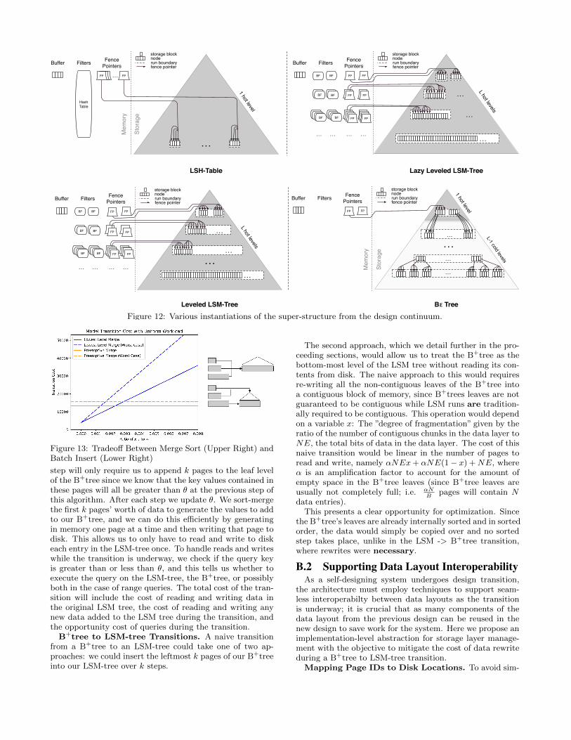
FPFP

Buffer Filters Fence Pointers

Mem

ory

Stor

age

HashTable

noderun boundaryfence pointer

storage block

1 hot level

LSH-Table

Buffer Filters Fence Pointers

FPBF

FPFPBFBF BFBF

noderun boundaryfence pointer

storage block

FPFPL hot levels

FPBF

…

FPFPBFBF FPFP …

… ………

BFBFBFBFBFBF

Lazy Leveled LSM-Tree

FPFPFPFP

…

FPFP

…

Buffer Filters Fence Pointers

FP

……

noderun boundaryfence pointer

storage block

…

1 hot level

L-1 cold levels

FP

Bε Tree

Buffer Filters Fence Pointers

FPBF

FPFP

BFBF BFBF

noderun boundaryfence pointer

storage block

FPFP

L hot levels

FPBF

FPFPBFBF FPFP

… ………

BFBFBFBFBFBF

Leveled LSM-Tree

FPFPFPFP

…

…

Mem

ory

Stor

age

…

…

…

…

Figure 12: Various instantiations of the super-structure from the design continuum.

Figure 13: Tradeoff Between Merge Sort (Upper Right) andBatch Insert (Lower Right)

step will only require us to append k pages to the leaf levelof the B+tree since we know that the key values contained inthese pages will all be greater than θ at the previous step ofthis algorithm. After each step we update θ. We sort-mergethe first k pages’ worth of data to generate the values to addto our B+tree, and we can do this efficiently by generatingin memory one page at a time and then writing that page todisk. This allows us to only have to read and write to diskeach entry in the LSM-tree once. To handle reads and writeswhile the transition is underway, we check if the query keyis greater than or less than θ, and this tells us whether toexecute the query on the LSM-tree, the B+tree, or possiblyboth in the case of range queries. The total cost of the tran-sition will include the cost of reading and writing data inthe original LSM tree, the cost of reading and writing anynew data added to the LSM tree during the transition, andthe opportunity cost of queries during the transition.

B+tree to LSM-tree Transitions. A naive transitionfrom a B+tree to an LSM-tree could take one of two ap-proaches: we could insert the leftmost k pages of our B+treeinto our LSM-tree over k steps.

The second approach, which we detail further in the pro-ceeding sections, would allow us to treat the B+tree as thebottom-most level of the LSM tree without reading its con-tents from disk. The naive approach to this would requiresre-writing all the non-contiguous leaves of the B+tree intoa contiguous block of memory, since B+trees leaves are notguaranteed to be contiguous while LSM runs are tradition-ally required to be contiguous. This operation would dependon a variable x: The ”degree of fragmentation” given by theratio of the number of contiguous chunks in the data layer toNE, the total bits of data in the data layer. The cost of thisnaive transition would be linear in the number of pages toread and write, namely αNEx+ αNE(1− x) +NE, whereα is an amplification factor to account for the amount ofempty space in the B+tree leaves (since B+tree leaves areusually not completely full; i.e. αN

Bpages will contain N

data entries).This presents a clear opportunity for optimization. Since

the B+tree’s leaves are already internally sorted and in sortedorder, the data would simply be copied over and no sortedstep takes place, unlike in the LSM -> B+tree transition,where rewrites were necessary.

B.2 Supporting Data Layout InteroperabilityAs a self-designing system undergoes design transition,

the architecture must employ techniques to support seam-less interoperabilty between data layouts as the transitionis underway; it is crucial that as many components of thedata layout from the previous design can be reused in thenew design to save work for the system. Here we propose animplementation-level abstraction for storage layer manage-ment with the objective to mitigate the cost of data rewriteduring a B+tree to LSM-tree transition.

Mapping Page IDs to Disk Locations. To avoid sim-

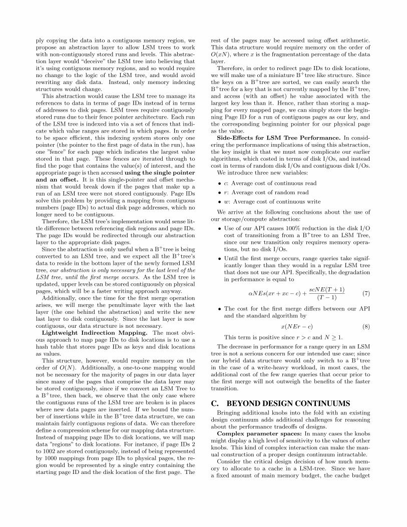
ply copying the data into a contiguous memory region, wepropose an abstraction layer to allow LSM trees to workwith non-contiguously stored runs and levels. This abstrac-tion layer would “deceive” the LSM tree into believing thatit’s using contiguous memory regions, and so would requireno change to the logic of the LSM tree, and would avoidrewriting any disk data. Instead, only memory indexingstructures would change.

This abstraction would cause the LSM tree to manage itsreferences to data in terms of page IDs instead of in termsof addresses to disk pages. LSM trees require contiguouslystored runs due to their fence pointer architecture. Each runof the LSM tree is indexed into via a set of fences that indi-cate which value ranges are stored in which pages. In orderto be space efficient, this indexing system stores only onepointer (the pointer to the first page of data in the run), hasone ”fence” for each page which indicates the largest valuestored in that page. These fences are iterated through tofind the poge that contains the value(s) of interest, and theappropriate page is then accessed using the single pointerand an offset. It is this single-pointer and offset mecha-nism that would break down if the pages that make up arun of an LSM tree were not stored contiguously. Page IDssolve this problem by providing a mapping from contiguousnumbers (page IDs) to actual disk page addresses, which nolonger need to be contiguous.

Therefore, the LSM tree’s implementation would sense lit-tle difference between referencing disk regions and page IDs.The page IDs would be redirected through our abstractionlayer to the appropriate disk pages.

Since the abstraction is only useful when a B+tree is beingconverted to an LSM tree, and we expect all the B+tree’sdata to reside in the bottom layer of the newly formed LSMtree, our abstraction is only necessary for the last level of theLSM tree, until the first merge occurs. As the LSM tree isupdated, upper levels can be stored contiguously on physicalpages, which will be a faster writing approach anyway.

Additionally, once the time for the first merge operationarises, we will merge the penultimate layer with the lastlayer (the one behind the abstraction) and write the newlast layer to disk contiguously. Since the last layer is nowcontiguous, our data structure is not necessary.

Lightweight Indirection Mapping. The most obvi-ous approach to map page IDs to disk locations is to use ahash table that stores page IDs as keys and disk locationsas values.

This structure, however, would require memory on theorder of O(N). Additionally, a one-to-one mapping wouldnot be necessary for the majority of pages in our data layersince many of the pages that comprise the data layer maybe stored contiguously, since if we convert an LSM Tree toa B+tree, then back, we observe that the only case wherethe contiguous runs of the LSM tree are broken is in placeswhere new data pages are inserted. If we bound the num-ber of insertions while in the B+tree data structure, we canmaintain fairly contiguous regions of data. We can thereforedefine a compression scheme for our mapping data structure.Instead of mapping page IDs to disk locations, we will mapdata ”regions” to disk locations. For instance, if page IDs 2to 1002 are stored contiguously, instead of being representedby 1000 mappings from page IDs to physical pages, the re-gion would be represented by a single entry containing thestarting page ID and the disk location of the first page. The

rest of the pages may be accessed using offset arithmetic.This data structure would require memory on the order ofO(xN), where x is the fragmentation percentage of the datalayer.

Therefore, in order to redirect page IDs to disk locations,we will make use of a miniature B+tree like structure. Sincethe keys on a B+tree are sorted, we can easily search theB+tree for a key that is not currently mapped by the B+tree,and access (with an offset) he value associated with thelargest key less than it. Hence, rather than storing a map-ping for every mapped page, we can simply store the begin-ning Page ID for a run of contiguous pages as our key, andthe corresponding beginning pointer for our physical pageas the value.

Side-Effects for LSM Tree Performance. In consid-ering the performance implications of using this abstraction,the key insight is that we must now complicate our earlieralgorithms, which costed in terms of disk I/Os, and insteadcost in terms of random disk I/Os and contiguous disk I/Os.

We introduce three new variables:

• c: Average cost of continuous read

• r: Average cost of random read

• w: Average cost of continuous write

We arrive at the following conclusions about the use ofour storage/compute abstraction:

• Use of our API causes 100% reduction in the disk I/Ocost of transitioning from a B+tree to an LSM Tree,since our new transition only requires memory opera-tions, but no disk I/Os.

• Until the first merge occurs, range queries take signif-icantly longer than they would in a regular LSM treethat does not use our API. Specifically, the degradationin performance is equal to

αNEs(xr + xc− c) +scNE(T + 1)

(T − 1)(7)

• The cost for the first merge differs between our APIand the standard algorithm by

x(NEr − c) (8)

This term is positive since r > c and N ≥ 1.

The decrease in performance for a range query in an LSMtree is not a serious concern for our intended use case; sinceour hybrid data structure would only switch to a B+treein the case of a write-heavy workload, in most cases, theadditional cost of the few range queries that occur prior tothe first merge will not outweigh the benefits of the fastertransition.

C. BEYOND DESIGN CONTINUUMSBringing additional knobs into the fold with an existing

design continuum adds additional challenges for reasoningabout the performance tradeoffs of designs.

Complex parameter spaces: In many cases the knobsmight display a high level of sensitivity to the values of otherknobs. This kind of complex interaction can make the man-ual construction of a proper design continuum intractable.

Consider the critical design decision of how much mem-ory to allocate to a cache in a LSM-tree. Since we havea fixed amount of main memory budget, the cache budget

must interact in multiple ways with other memory allocationbudgets.

In order to increase the size of the cache, we must strate-gize the best way to accordingly distribute the reductionin budget between the two other components that consumemain memory budget: the write buffer and Bloom filter.For instance, if we choose to take away from the size of thewrite buffer, we might assume that more queries will end uptouching more levels of the LSM-tree. Is this penalty offsetby having a larger cache? This depends on the hit rate ofthe cache, which ultimately depends on the query workload.

If we have a workload consisting of a small working set ofkeys dominating the majority of queries, then perhaps theresulting improvement from cache hits will produce an over-all improvement in performance. Alternatively, if we havea workload where the hot working set of keys is larger thanthe cache or even main memory, then we might find thatthe strategy of maximizing cache size turns into a bad one- e.g. a relatively small proportion of queries that cause acache miss and hit disk might be enough to sink overall per-formance because by reducing the space allocated to Bloomfilters we’ve increased their inaccuracy with higher false pos-itive rate (FPRs), meaning that each run is more likely toincur the full cost of a random I/O probe, rather than alower protected cost from effective Bloom filters.

If we had instead decided in the beginning to remove morememory from the Bloom filters rather than from the writebuffer, we’d encounter a different set of dilemmas in thedecision making process. On top of this, would increasingthe size of the write buffer be a good decision in the firstplace? We would need yet another set of criteria to be ableto make that determination.

Discretizing parameter spaces: We might have designknobs that are not smooth and continuous, but are made ofmany discrete options. Moreover, even continuous designknobs may need to be discretized in practice, to be naviga-ble.

Complex workloads: In real world scenarios we mighte.g. find that the hot working set of keys is not static butchanges over time, affecting performance with it [97].

For only a few parameters, we can end up with a situationwhere even hand-wavy intuition on tradeoffs becomes com-plicated. Knowing the exact parameters or the exact tippingpoints in which certain design strategies become better orworse is yet harder. At each turn, we encounter more sce-narios where the prevailing strategy is highly dependent onthe co-interaction of other design knobs and the nuances ofthe workload.

C.1 A Solution: Stochastic Gradient DescentWe see a path forward by combining machine learning

ideas with design continuum knowledge to create solutionsthat approach the optimal for a broader set of design de-cisions. The problem, to us, seems analogous to training amachine learning model:

The cost function that we’re minimizing is the dataaccess cost expressed in random I/O’s to storage, derivedfrom the design continuum.

The goal is to minimize the cost function, i.e. find theparameters that provide the lowest I/O cost for the givenset of queries.

The parameters are the cache size, the write buffer sizeand the bloom filter size.

The parameter space is only a subset of 3D space,because total memory is constrained. For example, if wewanted to increase both the cache size and the write buffersize we would have to decrease the bloom filter size.

The gradient functions are the estimated I/O savingsif we increase the memory by N bits for any single com-ponent. Following the gradients, one would expect to endup in a minima. While deriving these analytically is diffi-cult, we come up with reasonable estimates using the designcontinuum cost formulas.

The dataset we’re training the model on is a key-valueworkload, i.e. a set of queries. We automatically generateours from probabilistic models, but one could also use tracesof real systems, or perhaps a combination of both.

C.2 Stochastic WorkloadsTo avoid overfitting to a particular set of queries, we define

some workload classes as configurable probabilistic models.We can then generate an ordered sequence of point readsor updates (i.e. a workload) from any of these. We includemore complex, time-varying workloads (inspired by [97] and[11]) that attempt to mimic realistic settings.

For all the workloads, when we draw a particular key forthe first time we will insert it into the database as a write,and subsequently we will either look it up or update it withprobability w.

Uniform queries will be drawn uniformly from a set ofK keys. This is often one in which the cache is unhelpful,but in practice may be unrealistic. Nevertheless, this is thescenario that many analyses assume.

Round-Robin queries are drawn deterministically usingki = (i mod K), i.e. we iteratively draw each key in se-quence, then repeat. This represents another pathologicalscenario for a cache: a key that has been recently written orread is actually a contraindication we will access it again.

80-20 queries (considered in [24]) are drawn such that20% of the most recently inserted keys constitute 80% ofthe lookups. This is a simple model to observe the effects ofskew.

Zipf queries are distributed according to a zeta distribu-tion, with a parameter s which describes the skewness. Zipf-distributed queries are considered in [61] as another simpleproxy for realistically skewed queries.

Discover-Decay queries are distributed according to thefollowing stochastic process, inspired by the Chinese Restau-rant process [5] but with time decay: with every passing timestep, we draw a number of reads nr, writes nw, and updatesnu assuming queries arrive according to Poisson processeswith configurable rates:

nr ∼ Pois(λr)

nw ∼ Pois(λw)

nu ∼ Pois(λu)

Once we’ve drawn our nw new keys ki, we assign them aninitial popularity

θi ∼ Beta(aθ, bθ)

with a random decay rate

γi ∼ Beta(aγ , bγ),

which is the factor by which they exponentially decay eachsubsequent time step. At any time t, the popularity of

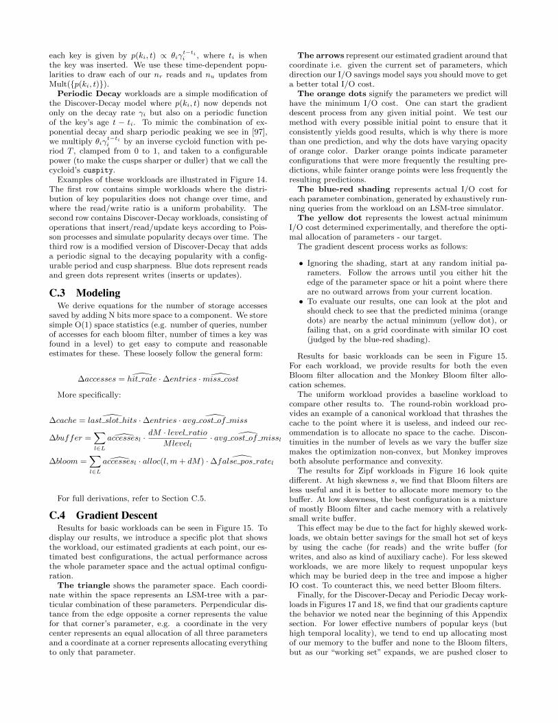
each key is given by p(ki, t) ∝ θiγt−tii , where ti is when

the key was inserted. We use these time-dependent popu-larities to draw each of our nr reads and nu updates fromMult({p(ki, t)}).

Periodic Decay workloads are a simple modification ofthe Discover-Decay model where p(ki, t) now depends notonly on the decay rate γi but also on a periodic functionof the key’s age t − ti. To mimic the combination of ex-ponential decay and sharp periodic peaking we see in [97],we multiply θiγ

t−tii by an inverse cycloid function with pe-

riod T , clamped from 0 to 1, and taken to a configurablepower (to make the cusps sharper or duller) that we call thecycloid’s cuspity.

Examples of these workloads are illustrated in Figure 14.The first row contains simple workloads where the distri-bution of key popularities does not change over time, andwhere the read/write ratio is a uniform probability. Thesecond row contains Discover-Decay workloads, consisting ofoperations that insert/read/update keys according to Pois-son processes and simulate popularity decays over time. Thethird row is a modified version of Discover-Decay that addsa periodic signal to the decaying popularity with a config-urable period and cusp sharpness. Blue dots represent readsand green dots represent writes (inserts or updates).

C.3 ModelingWe derive equations for the number of storage accesses

saved by adding N bits more space to a component. We storesimple O(1) space statistics (e.g. number of queries, numberof accesses for each bloom filter, number of times a key wasfound in a level) to get easy to compute and reasonableestimates for these. These loosely follow the general form:

∆accesses = hit rate ·∆entries · miss cost

More specifically:

∆cache = last slot hits ·∆entries · avg cost of miss

∆buffer =∑l∈L

accessesl ·dM · level ratio

Mlevell· avg cost of missl

∆bloom =∑l∈L

accessesl · alloc(l,m+ dM) · ∆false pos ratel

For full derivations, refer to Section C.5.

C.4 Gradient DescentResults for basic workloads can be seen in Figure 15. To

display our results, we introduce a specific plot that showsthe workload, our estimated gradients at each point, our es-timated best configurations, the actual performance acrossthe whole parameter space and the actual optimal configu-ration.

The triangle shows the parameter space. Each coordi-nate within the space represents an LSM-tree with a par-ticular combination of these parameters. Perpendicular dis-tance from the edge opposite a corner represents the valuefor that corner’s parameter, e.g. a coordinate in the verycenter represents an equal allocation of all three parametersand a coordinate at a corner represents allocating everythingto only that parameter.

The arrows represent our estimated gradient around thatcoordinate i.e. given the current set of parameters, whichdirection our I/O savings model says you should move to geta better total I/O cost.

The orange dots signify the parameters we predict willhave the minimum I/O cost. One can start the gradientdescent process from any given initial point. We test ourmethod with every possible initial point to ensure that itconsistently yields good results, which is why there is morethan one prediction, and why the dots have varying opacityof orange color. Darker orange points indicate parameterconfigurations that were more frequently the resulting pre-dictions, while fainter orange points were less frequently theresulting predictions.

The blue-red shading represents actual I/O cost foreach parameter combination, generated by exhaustively run-ning queries from the workload on an LSM-tree simulator.

The yellow dot represents the lowest actual minimumI/O cost determined experimentally, and therefore the opti-mal allocation of parameters - our target.

The gradient descent process works as follows:

• Ignoring the shading, start at any random initial pa-rameters. Follow the arrows until you either hit theedge of the parameter space or hit a point where thereare no outward arrows from your current location.• To evaluate our results, one can look at the plot and

should check to see that the predicted minima (orangedots) are nearby the actual minimum (yellow dot), orfailing that, on a grid coordinate with similar IO cost(judged by the blue-red shading).

Results for basic workloads can be seen in Figure 15.For each workload, we provide results for both the evenBloom filter allocation and the Monkey Bloom filter allo-cation schemes.

The uniform workload provides a baseline workload tocompare other results to. The round-robin workload pro-vides an example of a canonical workload that thrashes thecache to the point where it is useless, and indeed our rec-ommendation is to allocate no space to the cache. Discon-tinuities in the number of levels as we vary the buffer sizemakes the optimization non-convex, but Monkey improvesboth absolute performance and convexity.

The results for Zipf workloads in Figure 16 look quitedifferent. At high skewness s, we find that Bloom filters areless useful and it is better to allocate more memory to thebuffer. At low skewness, the best configuration is a mixtureof mostly Bloom filter and cache memory with a relativelysmall write buffer.

This effect may be due to the fact for highly skewed work-loads, we obtain better savings for the small hot set of keysby using the cache (for reads) and the write buffer (forwrites, and also as kind of auxiliary cache). For less skewedworkloads, we are more likely to request unpopular keyswhich may be buried deep in the tree and impose a higherIO cost. To counteract this, we need better Bloom filters.

Finally, for the Discover-Decay and Periodic Decay work-loads in Figures 17 and 18, we find that our gradients capturethe behavior we noted near the beginning of this Appendixsection. For lower effective numbers of popular keys (buthigh temporal locality), we tend to end up allocating mostof our memory to the buffer and none to the Bloom filters,but as our “working set” expands, we are pushed closer to

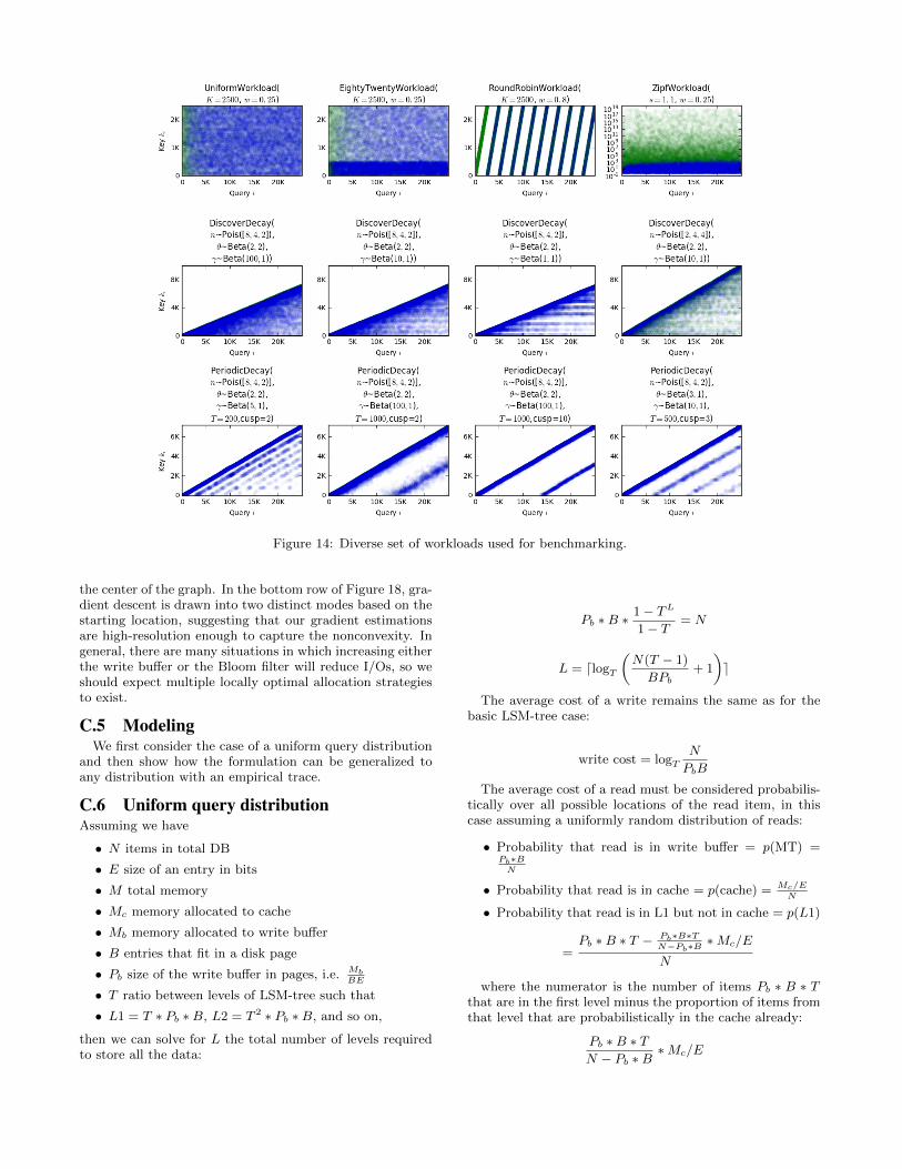
Figure 14: Diverse set of workloads used for benchmarking.

the center of the graph. In the bottom row of Figure 18, gra-dient descent is drawn into two distinct modes based on thestarting location, suggesting that our gradient estimationsare high-resolution enough to capture the nonconvexity. Ingeneral, there are many situations in which increasing eitherthe write buffer or the Bloom filter will reduce I/Os, so weshould expect multiple locally optimal allocation strategiesto exist.

C.5 ModelingWe first consider the case of a uniform query distribution

and then show how the formulation can be generalized toany distribution with an empirical trace.

C.6 Uniform query distributionAssuming we have

• N items in total DB

• E size of an entry in bits

• M total memory

• Mc memory allocated to cache

• Mb memory allocated to write buffer

• B entries that fit in a disk page

• Pb size of the write buffer in pages, i.e. MbBE

• T ratio between levels of LSM-tree such that

• L1 = T ∗ Pb ∗B, L2 = T 2 ∗ Pb ∗B, and so on,

then we can solve for L the total number of levels requiredto store all the data:

Pb ∗B ∗1− TL

1− T = N

L = dlogT

(N(T − 1)

BPb+ 1

)e

The average cost of a write remains the same as for thebasic LSM-tree case:

write cost = logTN

PbB

The average cost of a read must be considered probabilis-tically over all possible locations of the read item, in thiscase assuming a uniformly random distribution of reads:

• Probability that read is in write buffer = p(MT) =Pb∗BN

• Probability that read is in cache = p(cache) = Mc/EN

• Probability that read is in L1 but not in cache = p(L1)

=Pb ∗B ∗ T − Pb∗B∗T

N−Pb∗B∗Mc/E

N

where the numerator is the number of items Pb ∗ B ∗ Tthat are in the first level minus the proportion of items fromthat level that are probabilistically in the cache already:

Pb ∗B ∗ TN − Pb ∗B

∗Mc/E

Figure 15: Uniform and Round-Robin simulation resultsoverlaid with gradient estimates.

Figure 16: Zipf simulation results overlaid with gradient es-timates for s = 1.1 (lightly skewed) and s = 1.5 (highlyskewed).

and finally where the N − Pb ∗ B comes from the fact thatitems already in buffer (L0) are not allowed to occupy thecache.

Figure 17: Discover-Decay simulation results overlaid withgradient estimates for lightly skewed and highly skewed.

Figure 18: Periodic Decay simulation results overlaid withgradient estimates for variations in periodicity (T) and skew(Beta distribution parameters).

Therefore, given a uniform query distribution, the full ex-

pected cost in disk reads of a read is

E[Cuniform] = p(MT) ∗ 0 + p(cache) ∗ 0 +

L∑i=1

p(Li) ∗ i

=

L∑i=1

Pb ∗B ∗ T i − Pb∗B∗T i

N−Pb∗B∗Mc/E

N∗ i

C.7 Bloom FiltersThe previous analysis hasn’t yet accounted for the pres-

ence of Bloom filters, which reduce the likelihood we willunnecessarily access a larger level. For a Bloom filter ofk bits with h independent hash functions h1, h2, ...hh, theprobability that a given bit is still set to 0 after inserting nkeys is

(1− 1

k)n∗h

Then the probability of a false positive is

(1− (1− 1

k)n∗h)h ≈ (1− e−hn/k)h

We can minimize this over h to find the optimal number ofhash functions, which is h = ln(2)∗ k

n. Assuming that this is

the number of hash functions h we will use, the probabilityof a false positive as a function of the number of bits is then

(1− e−ln(2)∗k/n∗n/k)ln(2)∗ kn = (

1

2)ln(2)∗ k

n ≈ (.6185)kn

For an item in any level Li of the LSM-tree with i ≥ 2we can reduce the expected cost of accessing that item fromLi by the number of Bloom filter negatives at any level j < i.

Then the expected cost of accessing an item at Li is

i−1∑j=1

p(fpj) ∗ 1 + 1

Where p(fpj) is the probability of a false positive for thatkey at level j and 1 is the cost of actually accessing the itemat level i assuming fence pointers that lead us to the correctpage.

C.8 Cost with Bloom Filters - Base CaseAssuming a random distribution of reads, we now consider

also the probability that a Bloom filter allows us to ignorea level:Expected cost of read for an item in the tree =

p(mt) ∗ 0 + p(cache) + 0 +

L∑i=1

p(Li) ∗i−1∑j=1

p(fpj)

Expected cost for a null result read =∑Lj=1 p(fpj)

Given a total memory allocation M , the total number ofbits we can allocate to Bloom filters is M −Mc =

∑Li=1 mi

Then the total formula for the expected cost of a read in thetree is:

E[c] =∑Li=1

B∗P∗T i−Pb∗B∗Ti

N−Pb∗B∗Mc/E

N

·

[(i−1∑j=1

(.6185)mj

Pb∗B∗Tj

)+ 1

](9)

Whereas with a given percentage of null reads in the work-load pnull:

E[c] = (1− pnull)∑Li=1

Pb∗B∗T i−Pb∗B∗Ti

N−Pb∗B∗Mc/E

N

·

[(i−1∑j=1

(.6185)mj

Pb∗B∗Tj

)+ 1

]+ pnull

L∑j=1

p(fpj) (10)

E[c] =∑Li=1(1− pnull)

Pb∗B∗T i−Pb∗B∗Ti

N−Pb∗B∗Mc/E

N

·

[(i−1∑j=1

(.6185)mj

Pb∗B∗Tj

)+ 1

]+ pnull · p(fpi) (11)

C.9 Cost Gradients w. Bloom Filters - Gener-alized Distribution

C.9.1 Cache GradientNote that in the above, the workload specific factors are

the probability that a read is at any given level and the re-lated probability that any given item from a level is alreadyin the cache. To compute an empirical estimation of theprobability that any given item is in a level but not alreadyin the cache, we can simply keep statistics on the total num-ber of times a key was found in that level divided by thetotal number of (non-null) read queries executed. Then wecan consider the following simplification:

E[c] =∑Li=1(1− pnull)

[p(Li)− p(Li)

(N−PbB)∗Mc/E

]·

[(i−1∑j=1

(.6185)mj

Pb∗B∗Tj

)+ 1

]+ pnull · p(fpi) (12)

Taking the derivative with respect to the number of entriesin the cache, Mc/E, we get:

L∑i=1

−(1−pnull)p(Li)/(N−PbB)·

[(i−1∑j=1

(.6185)mj

Pb∗B∗Tj

)+ 1

]

Which is just the average cost of a read throughout thetree. Then, to keep statistics on how valuable we expect thecache to be, we maintain statistics on the average cost ofevery read performed in the window of interest.

C.9.2 Bloom Filter GradientsBecause the memory allocation problem is discrete any-

way, we consider the value of the Bloom filters as a finitedifference, that is the approximate value of any marginalbloom filter bit at level k will be E[c|mk + 1]−E[c|mk]. Inthis computation, all terms in the sums drop out except forthose concerning mj , and we are left with:

∑Li=k(1− pnull)

[p(Li)− p(Li)

(N−PbB)∗Mc/E

]·{[(

(.6185)mk+1

Pb∗B∗Tj

)+ 1

]−[(

(.6185)mk

Pb∗B∗Tj

)+ 1

]}+ pnull

((.6185)

mk+1

Pb∗B∗Tj − (.6185)mk

Pb∗B∗Tj

)(13)

Rearranging terms, we get:∑Li=k

[(1− pnull)

[p(Li)− p(Li)

(N−PbB)∗Mc/E

]+ pnull

]·(

(.6185)mk+1

Pb∗B∗Tj − (.6185)mk

Pb∗B∗Tj

)(14)

Where this is exactly the number of times the given bloomfilter is accessed times the difference in the theoretical falsepositive rates given memory allocations mj and mj + 1.Then, to keep statistics on how valuable we expect any givenBloom filter to be, we maintain statistics on the number oftimes every Bloom filter was accessed in the window of in-terest.

C.9.3 Write Buffer Gradient: GetsTo estimate the additional value of any marginal memory

in the write buffer with respect to reads, we must make anumber of simplifications, as Pb, the number of pages in thewrite buffer, factors into every term in this equation. Fur-ther, the interaction between Pb and most of the terms isnot available in closed form, in general. Rather, the crit-ical terms P (Li) we are empirically estimating. Then, forreasonably large values of N and Pb, we will assume thatthe Bloom filter false positive rate stays approximately thesame, as does the value of the cache. Then, we consider onlythe change in I/Os occurring from the altered probability ofany given element occurring in any level as a result of moreelements being in the write buffer. We can provide a simpleestimate of this by assuming that any items we add to thewrite buffer would have otherwise occurred in L1, and inthe resulting cascade, T i times that number of items will bemoved up into each level Li from the level below.

Then, an appropriate estimate of how useful any addi-tional space of memory in the write buffer is for reads issimply the resulting change in p(Li) for each level (that is,the number of hits we expect to see on the newly addedelements) ∗fpi for any level i 6= 0, as the original cost of ac-

cessing that element was∑ij=1 fpj + 1, and the new cost of

accessing is∑i−1j=1 fpj , the difference between which is just

fpi. For i = 0, the write buffer itself, the expected savingsper hits is exactly 1, as the item will be moved from havingan access cost of 1 to 0. To estimate how many additionaltimes L1 would be accessed if we instead allocated the fi-nal portion of the write buffer to L1, we keep statistics onhow often the final spots of the write buffer were accessedin a read. In practice, these spots are accessed only veryinfrequently, as the write buffer is accessed only a hand-ful of times at this stage before being flushed. This statisticmight be more helpful on a system with constant compactionrather than a full level flush. For the rest of the levels, wesimply assume the same hit rate per key as measured overthe existing keys on any level and multiply by the numberof elements we will be adding to calculate the expected ac-cesses to the new keys on each level. We then multiply by

the empirical rate of bloom filter false positives on the level.

C.9.4 Write Buffer Gradient: PutsFor the write buffer, we must additionally consider the

saved I/Os for the update/insert operations.

write cost = logTN

PbB

Taking the derivative with respect to PbB, the number ofitems in the buffer, we get 1

PbBIn discrete terms, this eval-

uates to logTPbBPbB+1

.

Unfortunately, this simplification only works if we can as-sume that memory is being allocated in page-size chunks andthat the workload has no duplicates. In practice, the numberof I/Os associated with reading and writing throughout themerging process is a stepwise function that depends on pagesize, as reading or writing one element from or to a page hasthe same I/O cost as reading or writing a full page. To sim-plify our analysis of the page size write savings, we consideronly a ratio of T = 2, and we begin by addressing the casewth no duplicates.

With no duplicates, the final number of elements at anylevel of the tree is a deterministic function of the number ofelements inserted as well as the level sizes. Then consideringthe empirical number of items inserted into the buffer aswell as the size of the original buffer, we can solve for thetheoretical final structure of an alternate LSM-tree that hada buffer of size PbB + 1.

Additionally, given the number of elements on any givenlevel, no duplicates, and an original buffer size PbB + 1, weknow the number of times each T i ∗ (PbB+ 1)-size chunk oneach level will have been read and written given the currentfullness of the level. We can then multiply these numbersof known chunk reads and writes by the ceiling of the sizeof those possible chunks (which, with ratio T = 2 will beT i ∗ (PbB + 1) and T i ∗ (PbB + 1) ∗ 2) divided by pagesize,B. This gives us a more realistic number in which additionsof less than a pagesize of memory are not helpful in I/Osavings.

Comparing the read and write costs of this theoretical treeto the empirical reads and writes accesses of the existing treegives us an expected I/O savings related to updates for thelarger tree.

We consider additionally the fact that I/O savings are ingeneral lessened by the number of duplicates inserted, asduplicates will not be merged across the full depth of thetree. To take this into account we also keep a statistic forthe total number of duplicates merged over the window ofinterest per level and use this to calculate the percentageof duplicates removed relative to total keys at each level.This factors in in several places. First, when computing thetheoretical allocation of keys in the final tree, we considerthe total number of items that would have come in to thebuffer from the empirical count and adjust this at each levelby the percentage that are expected to have been removed asduplicates. Further, when computing read and write I/Osduring merging, we expect that number of items writtenwhen the level is already half full should be decreased by theexpected number of duplicates removed among the two setsof keys. Again, the resulting I/O savings will be stepwise inpagesize. In particular, if the original size of the array wouldhave only been slightly into the final page, it will take veryfew duplicates to reduce the I/O count by 1, whereas if all

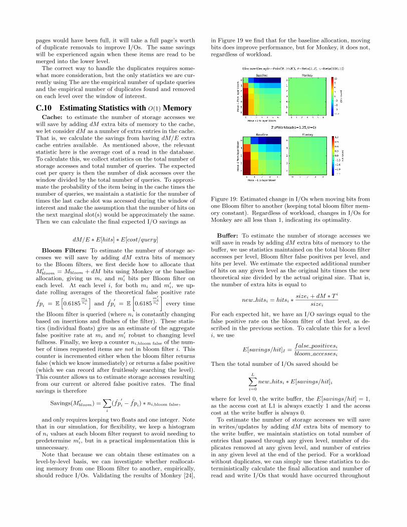
pages would have been full, it will take a full page’s worthof duplicate removals to improve I/Os. The same savingswill be experienced again when these items are read to bemerged into the lower level.

The correct way to handle the duplicates requires some-what more consideration, but the only statistics we are cur-rently using The are the empirical number of update queriesand the empirical number of duplicates found and removedon each level over the window of interest.

C.10 Estimating Statistics with O(1) MemoryCache: to estimate the number of storage accesses we

will save by adding dM extra bits of memory to the cache,we let consider dM as a number of extra entries in the cache.That is, we calculate the savings from having dM/E extracache entries available. As mentioned above, the relevantstatistic here is the average cost of a read in the database.To calculate this, we collect statistics on the total number ofstorage accesses and total number of queries. The expectedcost per query is then the number of disk accesses over thewindow divided by the total number of queries. To approxi-mate the probability of the item being in the cache times thenumber of queries, we maintain a statistic for the number oftimes the last cache slot was accessed during the window ofinterest and make the assumption that the number of hits onthe next marginal slot(s) would be approximately the same.Then we can calculate the final expected I/O savings as

dM/E ∗ E[hits] ∗ E[cost/query]

Bloom Filters: To estimate the number of storage ac-cesses we will save by adding dM extra bits of memoryto the Bloom filters, we first decide how to allocate thatM ′bloom = Mbloom + dM bits using Monkey or the baselineallocation, giving us mi and m′i bits per Bloom filter oneach level. At each level i, for both mi and m′i, we up-date rolling averages of the theoretical false positive rate

fpi = E[0.6185

mini

]and fp

′i = E

[0.6185

m′ini

]every time

the Bloom filter is queried (where ni is constantly changingbased on insertions and flushes of the filter). These statis-tics (individual floats) give us an estimate of the aggregatefalse positive rate at mi and m′i robust to changing levelfullness. Finally, we keep a counter ni,bloom false of the num-ber of times requested items are not in bloom filter i. Thiscounter is incremented either when the bloom filter returnsfalse (which we know immediately) or returns a false positive(which we can record after fruitlessly searching the level).This counter allows us to estimate storage accesses resultingfrom our current or altered false positive rates. The finalsavings is therefore

Savings(M ′bloom) =∑i

(fp′i − fpi) ∗ ni,bloom false,

and only requires keeping two floats and one integer. Notethat in our simulation, for flexibility, we keep a histogramof ni values at each bloom filter request to avoid needing topredetermine m′i, but in a practical implementation this isunnecessary.

Note that because we can obtain these estimates on alevel-by-level basis, we can investigate whether reallocat-ing memory from one Bloom filter to another, empirically,should reduce I/Os. Validating the results of Monkey [24],

in Figure 19 we find that for the baseline allocation, movingbits does improve performance, but for Monkey, it does not,regardless of workload.

Figure 19: Estimated change in I/Os when moving bits fromone Bloom filter to another (keeping total bloom filter mem-ory constant). Regardless of workload, changes in I/Os forMonkey are all less than 1, indicating its optimality.

Buffer: To estimate the number of storage accesses wewill save in reads by adding dM extra bits of memory to thebuffer, we use statistics maintained on the total bloom filteraccesses per level, Bloom filter false positives per level, andhits per level. We estimate the expected additional numberof hits on any given level as the original hits times the newtheoretical size divided by the actual original size. That is,the number of extra hits is equal to

new hitsi = hitsi ∗sizei + dM ∗ T i

sizei

For each expected hit, we have an I/O savings equal to thefalse positive rate on the bloom filter of that level, as de-scribed in the previous section. To calculate this for a leveli, we use

E[savings/hit]I =false positivesibloom accessesi

Then the total number of I/Os saved should be

L∑i=0

new hitsi ∗ E[savings/hit]i

where for level 0, the write buffer, the E[savings/hit] = 1,as the access cost at L1 is always exactly 1 and the accesscost at the write buffer is always 0.

To estimate the number of storage accesses we will savein writes/updates by adding dM extra bits of memory tothe write buffer, we maintain statistics on total number ofentries that passed through any given level, number of du-plicates removed at any given level, and number of entriesin any given level at the end of the period. For a workloadwithout duplicates, we can simply use these statistics to de-terministically calculate the final allocation and number ofread and write I/Os that would have occurred throughout

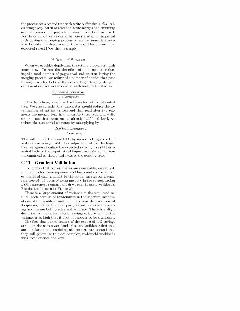
the process for a second tree with write buffer size + dM , cal-culating every batch of read and write merges and summingover the number of pages that would have been involved.For the original tree we can either use statistics on empiricalI/Os during the merging process or use the same determin-istic formula to calculate what they would have been. Theexpected saved I/Os then is simply

costtree − costtree+dM

When we consider duplicates, the estimate becomes muchmore noisy. To consider the effect of duplicates on reduc-ing the total number of pages read and written during themerging process, we reduce the number of entries that passthrough each level of our theoretical larger tree by the per-centage of duplicates removed at each level, calculated as

duplicates removeditotal entriesi

This then changes the final level structure of the estimatedtree. We also consider that duplicates should reduce the to-tal number of entries written and then read after two seg-ments are merged together. Then for those read and writecomponents that occur on an already half-filled level, wereduce the number of elements by multiplying by

1− duplicates removeditotal entriesi

This will reduce the total I/Os by number of page reads itmakes unnecessary. With this adjusted cost for the largertree, we again calculate the expected saved I/Os as the esti-mated I/Os of the hypothetical larger tree subtracted fromthe empirical or theoretical I/Os of the existing tree.

C.11 Gradient ValidationTo confirm that our estimates are reasonable, we ran 250

simulations for three separate workloads and compared ourestimates of each gradient to the actual savings for a sepa-rate tree with 8 bytes of extra memory in the correspondingLSM component (against which we ran the same workload).Results can be seen in Figure 20.

There is a large amount of variance in the simulated re-sults, both because of randomness in the separate instanti-ations of the workload and randomness in the execution ofits queries, but for the most part, our estimates of the aver-age savings are both precise and accurate. There is a slightdeviation for the uniform buffer savings calculation, but thevariance is so high that it does not appear to be significant.

The fact that our estimates of the expected I/O savingsare so precise across workloads gives us confidence first thatour simulation and modeling are correct, and second thatthey will generalize to more complex, real-world workloadswith more queries and keys.

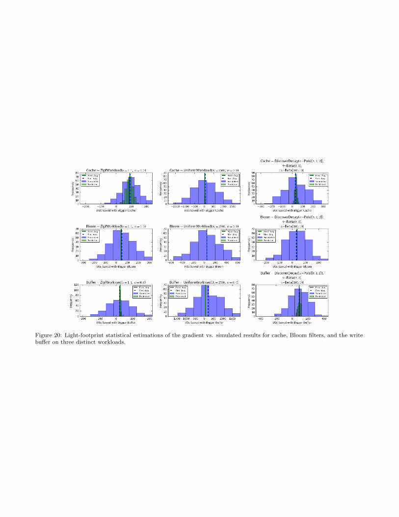
Figure 20: Light-footprint statistical estimations of the gradient vs. simulated results for cache, Bloom filters, and the writebuffer on three distinct workloads.