StratigrapheR: Concepts for Litholog Generation in R

CONTRIBUTED RESEARCH ARTICLES 153

StratigrapheR: Concepts for LithologGeneration in Rby Sébastien Wouters, Anne-Christine Da Silva, Frédéric Boulvain and Xavier Devleeschouwer

Abstract The StratigrapheR package proposes new concepts for the generation of lithological logs,or lithologs, in R. The generation of lithologs in a scripting environment opens new opportunitiesfor the processing and analysis of stratified geological data. Among the new concepts presented:new plotting and data processing methodologies, new general R functions, and computer-orienteddata conventions are provided. The package structure allows for these new concepts to be furtherimproved, which can be done independently by any R user. The current limitations of the package arehighlighted, along with the limitations in R for geological data processing, to help identify the bestpaths for improvements.

Introduction

StratigrapheR is a package implemented in the open-source programming environment R. Stratig-rapheR endeavors to explore new concepts to process stratified geological data. These concepts areprovided to answer a major difficulty posed by such data; namely a large amount of field observationsof varied nature, sometimes localized and small-scale, can carry information on large-scale processes.Visualizing the relevant observations all at once is therefore difficult. The usual answer to this problemin successions of stratified rocks is to report observations in a schematic form: the lithological log, orlitholog (e.g., Fig. 1). The litholog is an essential tool in sedimentology and stratigraphy and proves tobe equally invaluable in other fields such as volcanology, igneous petrology, or paleontology. Ideally,any data contained in a litholog should be available in a reproducible form. Therefore, the challengeat hand is what we would call "from art to useful data"; how can we best extract and/or process theinformation contained in a litholog, designed to be as visually informative as possible (see again Fig. 1).

28

29

30

31

32

33

34

44

45a

45b

45c

46

47

48

49

51

35

52a

52b

60a

60b

60c

61

HIATUS

lamellar stromatoporoids

branching stromatoporoids

lamellar tabulate corals

branching tabulate corals

brachiopods

crinoids

receptaculitids

small fenestrae

large fenestrae

bioclasts

Legend

brachiopods in lenses

lithoclasts

joints (clay seams)

The colours are similar to the coloursobserved on the field

Depth (m) Samples

Figure 1: Example of a computer-drawn litholog of calcareous rocks, modified from Humblet andBoulvain (2000) using vector graphics software (e.g., Inkscape, CorelDRAW, or Adobe Illustrator).

The R Journal Vol. 13/2, December 2021 ISSN 2073-4859

https://CRAN.R-project.org/package=StratigrapheR

https://CRAN.R-project.org/package=StratigrapheR


Lithologs can be hand-drawn, computer-drawn, or generated via ad hoc software tools. Drawnfigures can have unlimited precision and personalization. They are, however, time-consuming toproduce and ill-adapted for the extraction of data for further numerical analysis. Moreover, anymodification to drawn lithologs has to be performed manually. Ad hoc software tools such as theopen-source SedLog program (Zervas et al., 2009) or the SDAR R package (Ortiz et al., 2019) propose asolution to such short-comings by generating lithologs from geological data provided in a text format.The most common text format is the American Standard Code for Information Interchange -ASCII-.ASCII is used for the SedLog data format and for the Log ASCII Standard -LAS- (Heslop et al., 1999).The latter (LAS) is the data format used by the SDAR package.

A major advantage of ad hoc software tools is that any change in the data can automatically lead toan update in the display of the litholog. However, ad hoc software tools only permit a certain amountof personalization. The graphical output of ad hoc software tools, which can be obtained in vectorgraphics format (e.g., in the Scalable Vector Graphics [SVG] format), has to be post-processed in vectorgraphics software to add elements that are not supported by the data format. In SedLog, for instance,to add plots next to the litholog (i.e., to visualize quantified analytical values and their relation to thelithological features) the plots need to be generated separately and then added manually along thelitholog in vector graphics software. SedLog does permit a certain amount of personalization, but onlyfor the lithological symbology, by giving the user the option of adding self-made symbology (e.g., toshow the position of paleontological or sedimentological features). In the SDAR package, the onlydata automatically displayable are Gamma Ray spectrometry values, and the symbology (for lithology,fossils, etc.) cannot be personalized.

Generally speaking, the graphical style of the lithologs generated by ad hoc software tools isdifficult to personalize entirely. To do so, each functionality has to be modular, which is better done ina scripting language such as R. Yet, the SDAR package, although coded in R, is not modular. All theplotting is made using a single function. Any personalization feature would need to be explicitly codedinto that function, which would be a never-ending task. Moreover, ad hoc software tools are difficultto update and improve. Adding new functionalities or maintaining the software for compatibility withnew operating systems, for example, usually falls on the shoulders of the developers of that software.

The StratigrapheR package is presented here as a new mean to generate lithologs. It provides acomplementary approach to the existing methodologies and circumvents the aforementioned problems.StratigrapheR is designed not around a specific data format but on general tools able to deal withdifferent formats. This opens a way of processing the geological data through a scripting languagewhich has a large potential to evolve. StratigrapheR shows that symbiosis between automation andpersonalization is achievable for litholog generation. As it stands, the package does not meet the "fromart to useful data" challenge entirely. However, it is a proof of concept showing that, despite the artisticnature of lithologs, they can be based on usable digital data, or that conversely, usable data can beextracted from drawn lithologs.

StratigrapheR is coded in R, which disposes of automated package checks (Wickham, 2015) and isitself updated regularly. This is one mechanism against the inevitable obsolescence of the functionali-ties. Similarly, as the StratigrapheR package is structured in distinct basic functions, implementingnew functionalities (or updating existing ones) can be done more easily by any user. Furthermore,the processing of geological data, whether to generate lithologs or for any other procedure (amongothers plotting proxies, applying moving averages on these proxies, or performing spectral analysis),can directly be performed in R (see, for instance, the paleotree package for paleontology (Bapst,2012), the IsoplotR package for geochronology (Vermeesch, 2018), or the hht (Bowman and Lees,2013), astrochron (Meyers, 2014), biwavelet (Gouhier et al., 2019) and DecomposeR (Wouters, 2020)packages for spectral analysis). This means that the entire data treatment and visualization could beperformed in a single scripting environment: R.

The main concepts for the use of StratigrapheR are presented in this paper. The current limitationsof StratigrapheR and R for the processing of geological data are also highlighted to give an idea ofthe obstacles that the future developers will need to overcome to make R a better tool for geologicaldata processing. Throughout the paper, examples are provided on how to make lithologs and howto process geological data. They can be run in R (you can download R here); the current version ofStratigrapheR (1.2.3) works only on R 4.0 or higher versions. A GitHub repository is available athttps://github.com/sewouter/StratigrapheR, where outside users can suggest improvements andprovide feedback. The free RStudio interface is advised to use StratigrapheR in the R environment.The StratigrapheR package can be installed by typing:

install.packages("StratigrapheR")

To be used, the StratigrapheR package has to be loaded each time R or RStudio are opened, viathe following code:

library(StratigrapheR)


http://www.sedlog.com/

https://CRAN.R-project.org/package=SDAR

https://CRAN.R-project.org/package=paleotree

https://CRAN.R-project.org/package=IsoplotR

https://CRAN.R-project.org/package=hht

https://CRAN.R-project.org/package=astrochron

https://CRAN.R-project.org/package=biwavelet

https://CRAN.R-project.org/package=DecomposeR

https://www.r-project.org/

https://github.com/sewouter/StratigrapheR

https://rstudio.com/products/rstudio/#rstudio-desktop


Data importation and processing

Data of any form can easily be imported using basic R functions, such as read.table() or readLines()for text files. Excel files can be downloaded using, for instance, the read.xlsx() function from thexlsx package (Dragulescu and Arendt, 2020). We advise putting any tabular data into data frame form(i.e., a table), which can be done via the data.frame() function.

As stratigraphic data can be found in an interval form (e.g., a specific strata between 25 and 30 min a record, or the Jurassic between ca. 200 and ca. 145 million years ago), a formal scheme to dealwith such data is provided: the ’lim’ object (named after the xlim and ylim parameters that define theboundaries of plots in common R graphical functions) and a suite of functions that are associated to limobjects. The idea is to set a logical data format for intervals and to be able to manipulate these intervalsin R. The lim objects are made via the as.lim() function by providing boundaries in the form of thel and r arguments, which respectively stand for left and right boundaries. The actual order of theboundaries is irrelevant to avoid unnecessary data cleaning (which is the reason why ’left’ and ’right’were chosen as a convention rather than ’up’ and ’down’). Each interval can be identified using the idargument. Providing the upper and lower boundaries allows taking gaps into account in lithologs,contrary to simply providing the thickness of layers (also called beds). Whether the boundaries areincluded in the interval can be determined via the b argument, which defines the boundary rules. Thisis an abstract feature, especially for geology purposes, because it is usually of negligible importancewhether the infinitesimal position of a boundary is included in a given interval. However, taking thisinto account is critical to explicitly describe the behavior of intervals. This can be used, for instance, toassign an interval to a sample located at the common boundary between two intervals that do notoverlap otherwise. By providing a boundary rule, it can be explicitly assigned to only one of the twointervals, none of them, or both of them. The boundary rule is expressed by characters, and can beset to "[]" (or "closed") to include both boundary points, "][" (or "()", and "open") to exclude bothboundary points, "[[" (or "[)", "right-open" and "left-closed") to include only the left boundarypoint, and "]]" (or "(]", "left-open",and "right-closed") to include only the right boundary point.The left element (e.g., the [ of "[]") stands for the left boundary (not necessarily the lowest one), whilethe right element (e.g., the ] of "[]") stands for the right boundary (not necessarily the highest one).We illustrate how to visualize intervals with the following code (note: graphics generated by code inthe article are shown directly after the code that generates them):

interval <- as.lim(l = c(0,1,2), r = c(0.5,2,2.5), # Make a lim objectid = c("Int. 1","Int.2","Int.3"))

interval # print what is in the lim object#> $l#> [1] 0 1 2#> $r#> [1] 0.5 2.0 2.5#> $id#> [1] "Int. 1" "Int.2" "Int.3"#> $b#> [1] "[]" "[]" "[]"

# Visualization of the lim objectplot.new()plot.window(ylim = c(-0.5, 2.5), xlim = c(0, 2.5))axis(3, pos = 1.5, las = 1)

infobar(ymin = 0, ymax = 1, xmin = interval$l, xmax = interval$r,labels = c(interval$id), srt = 0)

0.0 0.5 1.0 1.5 2.0 2.5

Int. 1 Int.2 Int.3


https://CRAN.R-project.org/package=xlsx


Functions are provided to characterize the relationships of intervals with each other: are.lim.nonunique()checks whether the intervals are of non-zero thickness (e.g., unlike [1,1]), are.lim.nonadjacent()checks if the intervals do not share any adjacent boundaries, and are.lim.distinct() checks whetherthe intervals are not overlapping. The simp.lim() function is provided to merge adjacent and/oroverlapping intervals having identical IDs. The flip.lim() function is provided to find the com-plementary intervals of a set of intervals (i.e., the gaps). The mid.lim() function provides a way todefine intervals in between data points. If all different intervals are strictly non-overlapping for allvalues (for instance, the intervals [0,20[ and [20, 100] are non-overlapping and therefore 20 is uniquelyrepresented by the second interval), the in.lim() function can be used to find which values belong towhich respective intervals. Typically, such functions can be used to craft stratigraphic intervals (suchas magnetochrons or stages) and determine the beds or samples that are in or outside them.

General plotting considerations

The first challenge when plotting a litholog is its size: a litholog needs to be detailed at a small scale(typically at the centimeter scale for high precision) while spanning the entirety of a record (up tohundreds of meters). This makes lithologs sometimes quite extended. This is problematic consideringthat the classical R graphic window is not adapted to visualize anything exceeding the size of thecomputer screen. To remedy this problem, the pdfDisplay() function is here introduced, which drawsplots directly in a PDF (Portable Document File) document and opens it in the computer’s default PDFreader. This PDF document can have any size desired by the user, and therefore, allows visualizing allthe details of a very long litholog. This is illustrated by the code here below, which draws a verticallystanding stickman. Depending on the screen, this vertical stickman could be difficult to visualizewithout pdfDisplay().

To avoid having to close the PDF reader at each change of the plot (as most PDF readers do notpermit changes to the PDF file while it is displayed), each new PDF can be named differently: eachnew document version will have its name be followed by ’_(i)’, where i is the version number (e.g.,test_(1).pdf, test_(2).pdf, etc.). This practice is here referred as tracking the version number. It isnoteworthy to cite the free Sumatra PDF software, which is available for Windows operating systems,and lets PDF files be modified while still displaying them without the trick of having to change the filename. In that case, the tracking of the version numbers can be canceled by setting the track parameterto FALSE. PDF files generated by pdfDisplay() can easily be imported into vector graphics software.The pdfDisplay() function also allows for the direct generation of an SVG file. pdfDisplay() is awrapper of the more basic pdf() function (i.e., its code is based on the pdf() function); other PDFgenerating functions could be used interchangeably.

To make plots starting from an empty background, we advise using the plot.new() and plot.window()functions, which are of lower level (i.e., more basic) than the plot() function. They are used to create acompletely empty plotting environment in which to add the litholog. To add axes, the axis() functionis a versatile tool, which can be replaced by the minorAxis() function provided in StratigrapheR toadd minor axis ticks. The minorAxis() function is itself a wrapper of the axis() function.

graphical_function <- function() # Graphical function needed by pdfDisplay{

opar <- par()$mar # Save initial graphical parameterspar(mar = c(0,3,0,1)) # Change the margins of the plot

plot.new() # Open a new plotplot.window(xlim = c(-0.2, 1.2), ylim = c(-5, 1)) # Define plot coordinatesminorAxis(2, at.maj = seq(-5, 1, 0.5), n = 5, las = 1) # Add axispoints(c(0.25, 0.75), c(0.75, 0.75), pch = 19)polygon(c(0.1, 0.25, 0.75, 0.9, 0.75, 0.25, NA,

0, 0.25, 0.75, 1, 0.75, 0.25),c(0.5, 0.25, 0.25, 0.5, 0.4, 0.4, NA,0.5, 0, 0, 0.5, 1, 1), lwd = 2)

lines(x = c(0.5, 0.5, NA, 0, 0.2, 0.5, 0.8, 1, NA,0, 0.2, 0.5, 0.9, 1.2),

y = c(-0.25, -3, NA, -5, -4, -3, -4, -5, NA,-2.5, -1.5, -1, -0.75, 0.25), lwd = 2)

par(mar = opar) # Restore initial graphical parameters}

pdfDisplay(graphical_function(),"graphical_function", width = 3.5, height = 10)


https://www.sumatrapdfreader.org/free-pdf-reader.html


−5.0

−4.5

−4.0

−3.5

−3.0

−2.5

−2.0

−1.5

−1.0

−0.5

0.0

0.5

1.0

Adding every element of the lithologs symbology uses a very basic data format for polylines andpolygons, which are respectively drawn using the multigons() and multilines() functions. Thesenovel functions allow precise control of graphical parameters when drawing multiple polygons andpolylines. These functions require an identification argument i, similar for each point of a singlepolygon or polyline, and the x and y coordinates of each point. The following code shows the use ofthe multigons() and multilines() functions:

i <- c(rep("A1",6), rep("A2",6), rep("A3",6)) # Polygon IDsx <- c(1,2,3,3,2,1,2,3,4,4,3,2,3,4,5,5,4,3) # x coordinatesy <- c(1,2,3,4,5,6,1,2,3,4,5,6,1,2,3,4,5,6) # y coordinates

plot.new()plot.window(xlim = c(0,6), ylim = c(0,7))

multigons(i, x, y,front = "A2", # This gets the polygon A2 in front of all othersdensity = c(NA, 5, 10), # Shading line densityscol = "grey20", # Shading line color; one value means all polygons

# are subject to this graphical parametercol = c("black", "grey80", "white"), # Background colorlwd = 2, # Width of border linesslty = 2, slwd = 1) # Shading lines type and width



i <- c(rep("A1",6), rep("A2",6), rep("A3",6)) # Lines IDsx <- c(1,2,3,3,2,1,4,5,6,6,5,4,7,8,9,9,8,7) # x coordinatesy <- c(1,2,3,4,5,6,1,2,3,4,5,6,1,2,3,4,5,6) # y coordinates

plot.new()plot.window(xlim = c(0,10), ylim = c(0,7))

multilines(i, x, y,j = c("A3", "A1", "A2"), # j controls the order of the graphical

# parameters applied to each named line:lty = c(1,2,3), lwd = 2, # e.g., lty = 1 (solid line) is applied

# to "A3", the line at the righttype = c("l", "o", "o"),pch = c(NA,21,24), cex = 1, bg = "black")

●

●

●

●

●

●

The pointsvg() function is provided in StratigrapheR to import groups of polygons and polylinesdrawn in vector graphics software, under specific conditions: firstly, the drawing needs to be inSVG format; secondly, the pointsvg() function is only able to identify objects of class "line", "rect","polygon", and "polyline" in the SVG file. The reason for this is that only these types of objectsare simple lines, and polygons made of nodes linked together by straight lines. This means thatpointsvg() is not able to recognize all the objects present in an SVG file. Furthermore, pointsvg()only identifies the coordinates of each objects, regroups them into separate polygons and polylineobjects, and in which order to plot them. All other graphical parameters, such as color or line thickness,are not taken into account. These parameters have to be specified in the drawing functions. Objectsobtained using pointsvg() on SVG files can be added using the framesvg() or centresvg() functions,which respectively add the object within a given frame or center the object on a given point.

svg.file.directory <- tempfile(fileext = ".svg") # Creates temporary filewriteLines(example.ammonite.svg, svg.file.directory) # Writes svg in the file

ammonite.drawing <- pointsvg(file = svg.file.directory) # Read svg

plot.new()plot.window(xlim = c(-2, 5), ylim = c(-2, 2))axis(1)axis(2, las = 2)

centresvg(ammonite.drawing, # Objectx = c(3,0), y = 0, # Coordinates for centeringxfac = 2, yfac = 2, # Dimension stretching factorscol = c("grey","white")) # Graphical parameters

−2 −1 0 1 2 3 4 5

−2

−1

0

1

2



It should be noted that repetitions of the same SVG object can be generated by a single call ofthe framesvg() or centersvg() functions. This facilitates the automation of the litholog generation.Modifications of the SVG objects can also be accomplished using the changesvg() function, whichenables, among other things, to change the order of plotting of the polylines and polygons, removesome of them, or invert the figure in x and/or y. The framesvg() or centersvg() can also output thedrawing with modified coordinates, which can be plotted using placesvg() (see, for instance, thecode of the last example).

Generating lithologs

The data to make lithologs can be provided in the form shown in Table 1.

id l r h colour litho

B1 0 1 3 grey SB2 1 3 4 grey LB3 3 4 5 black CB4 4 9 4 white LB5 9 11 4 white L... ... ... ... ... ...

Table 1: Example of a data frame (bed.example in StratigrapheR) providing information for each bed:id identifies each bed, l and r provide the boundaries, h the hardness, and the color is provided alongwith a code for lithology (S for shale, L for limestone, C for chert). The only strict convention is that l, r,and h need to be numerical values.

From such data, basic lithologs made of rectangles can be generated as a simple basis. They are thestarting point for making more complicated lithologs in StratigrapheR. The coordinates of the pointsmaking up the rectangles can be computed through the litholog() function, which only needs theposition of the boundaries of the beds, their ’hardness’, and an ID. Text can be added to each bed usingthe bedtext() function, which can be used to include the ID or the name of the bed (e.g., id in Table 1).

The output of the litholog() function can be provided to multigons() to draw the log. Asymbology for different types of rocks (or any other information that the symbology is meant toprovide) can be set up using the color fill and the shading. Providing a given symbology for eachpolygon is performed by joining the table containing the information about each bed to a tableattributing symbology to rock type. We advise the use of the left_join() function in the dplyrpackage (Wickham et al., 2020) for this procedure.

basic.log <- litholog(l = bed.example$l, # This creates a data table ofr = bed.example$r, # rectangles coordinates for ah = bed.example$h, # basic lithologi = bed.example$id)

legend <- data.frame(litho = c("S", "L", "C"), # This creates acol = c("grey30", "grey90", "white"), # data table fordensity = c(30, 0,10), # the symbologyangle = c(180, 0, 45), stringsAsFactors = FALSE)

View(legend)

# left_join in the dplyr package merges the symbology with the table of beds:bed.legend <- dplyr::left_join(bed.example,legend, by = "litho")

View(bed.legend)


https://CRAN.R-project.org/package=dplyr


plot.new()plot.window(xlim = c(0,6), ylim = c(-1,77))minorAxis(2, at.maj = seq(0, 75, 5), n = 5)

# Plotting of the polygons making the litholog,# with corresponding symbology:multigons(basic.log$i, x = basic.log$xy, y = basic.log$dt,

col = bed.legend$col,density = bed.legend$density,angle = bed.legend$angle)

# Writing the name of beds, only in beds thick enoughbedtext(labels = bed.example$id, l = bed.example$l, r = bed.example$r,

x = 0.5, # x position where to center the textymin = 3) # text is not added in beds thinner than ymin

0

5

10

15

20

25

30

35

40

45

50

55

60

65

70

75

B4

B8

B13

B17

B22

B26

B31

B35



To add more complicated beds, the user can add SVG drawings instead of drawing the rectanglesthrough multigons(), as shown earlier. This is, however, a time-consuming procedure as each bedhas to be imported separately. The weldlog() function can be used to automate the personalization ofbed boundaries. It needs to be provided as a polyline, either from R itself (e.g., a sinusoid) or from anSVG file.

# Code repeated from earlier examples ----basic.log <- litholog(l = bed.example$l, r = bed.example$r,

h = bed.example$h, i = bed.example$id)legend <- data.frame(litho = c("S", "L", "C"), density = c(30, 0,10),

col = c("grey30", "grey90", "white"),angle = c(180, 0, 45), stringsAsFactors = FALSE)

bed.legend <- dplyr::left_join(bed.example,legend, by = "litho")# ----

# Generation of the boundaries, either sinusoidal or from drawings ---s1 <- sinpoint(5,0,0.5,nwave = 1.5)s2 <- sinpoint(5,0,1,nwave = 3, phase = 0)s3 <- framesvg(example.liquefaction, 1, 4, 0, 2, plot = FALSE, output = TRUE)

# Visualizing the s3 boundary, i.e., the liquefaction sedimentary feature ----plot(s3$x, s3$y, cex.axis = 1.2, lwd = 2,

type = "l", ylab = "", xlab = "", bty = "n", las = 1)

1.0 1.5 2.0 2.5 3.0 3.5 4.0

0.0

0.5

1.0

1.5

2.0

# Welding the boundaries to the basic litholog ----final.log <- weldlog(log = basic.log,

dt = boundary.example$dt, # Position of the boundaries# to be changed

seg = list(s1 = s1, s2 = s2, s3 = s3), # list of segmentsj = c("s1","s1","s1","s3", # Attributing the segments to

"s2","s2","s1"), # the respective bed boundaries# to be changed

warn = F)

# Visualizing the resulting litholog (similarly to earlier code) ----plot.new()plot.window(xlim = c(0,6), ylim = c(-1,77))minorAxis(2, at.maj = seq(0, 75, 5), n = 5, las = 1)

multigons(final.log$i, x = final.log$xy, y = final.log$dt,col = bed.legend$col,density = bed.legend$density,angle = bed.legend$angle)

bedtext(labels = bed.example$id, l = bed.example$l, r = bed.example$r,x = 0.75, ymin = 3)



0

5

10

15

20

25

30

35

40

45

50

55

60

65

70

75

B4

B8

B13

B17

B22

B26

B31

B35

We see that the thickness of beds can vary. Therefore, a bed boundary can actually vary within agiven interval. This raises the question of how to document the position of the bed boundaries in datatables that would only have 2 values for the boundaries (lower and upper) rather than 4 (upper andlower interval of variation for the lower boundary, and upper and lower interval of variation for theupper boundary) or even more (detailing the exact form of the boundaries). We propose a conventionfor the data tables to be used for the generation of lithologs: the positions of the bed boundaries thatare defined in the quantified data have to match in a litholog with the positions of the boundariesof the beds on the axis side of the litholog (usually the left side for single logs). The axis side of thelitholog is ideal: it follows a straight vertical line, by an implicit convention followed by the largemajority of geologists.

Extra stratigraphic or lithological information, such as geomagnetic chrons, rock color, etc., canbe added using the infobar() function. Any information that can be conveyed by text, such as thepositions of samples, can be added using the axis() or text() functions.


h = bed.example$h, i = bed.example$id)legend <- data.frame(litho = c("S", "L", "C"), density = c(30, 0,10),

col = c("grey30", "grey90", "white"),angle = c(180, 0, 45), stringsAsFactors = FALSE)

bed.legend <- dplyr::left_join(bed.example,legend, by = "litho")s1 <- sinpoint(5,0,0.5,nwave = 1.5)s2 <- sinpoint(5,0,1,nwave = 3, phase = 0)s3 <- framesvg(example.liquefaction, 1, 4, 0, 2, plot = FALSE, output = TRUE)final.log <- weldlog(log = basic.log, dt = boundary.example$dt,

seg = list(s1 = s1, s2 = s2, s3 = s3),j = c("s1","s1","s1","s3","s2","s2","s1"), warn = F)



# Visualizing the resulting litholog (similarly to earlier code) ----plot.new()plot.window(xlim = c(-1.5,8), ylim = c(-1,81))minorAxis(2, at.maj = seq(0, 75, 5), n = 5, las = 1)



# Making a data table for the symbology of magnetochronslegend.chron <- data.frame(polarity = c("N", "R"),

bg.col = c("black", "white"),text.col = c("white", "black"),stringsAsFactors = FALSE)

# Merging symbology with a data table of chronschron.legend <- dplyr::left_join(chron.example, legend.chron, by = "polarity")

# Plotting the chrons with the given symbologyinfobar(-1.5, -1, chron.legend$l, chron.legend$r,

labels = chron.legend$polarity,m = list(col = chron.legend$bg.col),t = list(col = chron.legend$text.col),srt = 0)

# Adding color informationcolour <- bed.example$colourcolour[colour == "darkgrey"] <- "grey20"colour[colour == "brown"] <- "tan4"

# Plotting the color next to the lithologinfobar(-0.25, -0.75, bed.example$l, bed.example$r,

m = list(col = colour))

text(-0.5, 79, "Colour", srt = 90)text(-1.25, 79, "Magnetochrons", srt = 90)

axis(4, at = proxy.example$dt, labels = proxy.example$name,pos = 6, lwd = 0, lwd.ticks = 1, las = 1)



0

5

10

15

20

25

30

35

40

45

50

55

60

65

70

75

B2

B4

B5

B7

B8

B9

B11

B13

B14

B16

B17

B18

B20

B22

B23

B25

B26

B27

B29

B31

B32

B34

B35

B36

N

R

N

Col

our

Mag

neto

chro

ns

EXA 1EXA 2EXA 3EXA 4EXA 5EXA 6EXA 7EXA 8EXA 9EXA 10EXA 11EXA 12EXA 13EXA 14EXA 15EXA 16EXA 17EXA 18EXA 19EXA 20EXA 21EXA 22EXA 23EXA 24EXA 25EXA 26EXA 27EXA 28EXA 29EXA 30EXA 31EXA 32EXA 33EXA 34EXA 35EXA 36EXA 37EXA 38EXA 39EXA 40EXA 41EXA 42EXA 43EXA 44EXA 45EXA 46EXA 47EXA 48EXA 49EXA 50EXA 51EXA 52EXA 53EXA 54EXA 55EXA 56EXA 57EXA 58EXA 59EXA 60EXA 61EXA 62EXA 63EXA 64EXA 65EXA 66EXA 67EXA 68EXA 69EXA 70EXA 71EXA 72EXA 73EXA 74EXA 75EXA 76

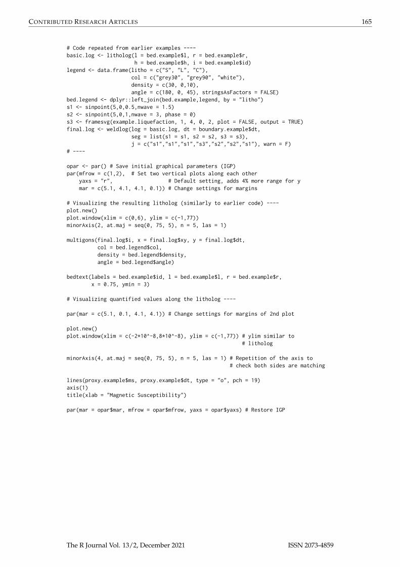
Other plots can be drawn along the litholog. Great care should be taken to ensure that the depthaxis is identical in all plots. To ensure that, two components have to be taken into account: theylim argument of plot.window() or plot() (for vertical logs, otherwise the xlim argument), and thegraphical parameters defined by the par() function, especially the yaxs (for vertical logs, otherwisexaxs) and the mar arguments. The ylim argument controls the range of the axis, but the exact rangewill depend on the yaxs argument. Indeed, the default setting of yaxs is "r", which stands for regular,and means that the data range defined by ylim is extended by 4 percent at each end. Such extensioncan be unwanted in very long lithologs. Alternatively, the yaxs argument can be set as "i", whichstands for ’internal’, and prevents the extension of the range defined by ylim. The mar argumentcontrols the margin size of the plotting zone. To add plots along the litholog, a simple way is to usethe mfrow argument in the par() function to define several plotting areas, which will be used by thesuccessively called plots.




h = bed.example$h, i = bed.example$id)legend <- data.frame(litho = c("S", "L", "C"),

col = c("grey30", "grey90", "white"),density = c(30, 0,10),angle = c(180, 0, 45), stringsAsFactors = FALSE)



# ----

opar <- par() # Save initial graphical parameters (IGP)par(mfrow = c(1,2), # Set two vertical plots along each other

yaxs = "r", # Default setting, adds 4% more range for ymar = c(5.1, 4.1, 4.1, 0.1)) # Change settings for margins

# Visualizing the resulting litholog (similarly to earlier code) ----plot.new()plot.window(xlim = c(0,6), ylim = c(-1,77))minorAxis(2, at.maj = seq(0, 75, 5), n = 5, las = 1)



# Visualizing quantified values along the litholog ----

par(mar = c(5.1, 0.1, 4.1, 4.1)) # Change settings for margins of 2nd plot

plot.new()plot.window(xlim = c(-2*10^-8,8*10^-8), ylim = c(-1,77)) # ylim similar to

# litholog

minorAxis(4, at.maj = seq(0, 75, 5), n = 5, las = 1) # Repetition of the axis to# check both sides are matching

lines(proxy.example$ms, proxy.example$dt, type = "o", pch = 19)axis(1)title(xlab = "Magnetic Susceptibility")

par(mar = opar$mar, mfrow = opar$mfrow, yaxs = opar$yaxs) # Restore IGP



0

5

10

15

20

25

30

35

40

45

50

55

60

65

70

75

B4

B8

B13

B17

B22

B26

B31

B35

0

5

10

15

20

25

30

35

40

45

50

55

60

65

70

75

●●●

●●

●●

●●

●●

●●●

●●

●●●

●●

●●

●●

●●

●●

●●●●

●●

●●●

●●

●●

●●

●●

●●

●●●●

●●

●●●

●●

●●

●●

●●

●●

●●●●

●●

●●

●

−2e−08 2e−08 6e−08

Magnetic Susceptibility

A legend plot can be generated using the nlegend() function. The basic idea is to make a subplotfor each symbol (using the par() function, for instance), in which the nlegend() function calls a newplot leaving free space for the symbol (included in [-1, 1], both for x and y coordinates), and adds thetext description. This scheme improves automation, e.g., by simplifying the symbol generation of rocktypes in a function as shown in the code below:

legend <- data.frame(litho = c("S", "L", "C"), # Symbologycol = c("grey30", "grey90", "white"), # data tabledensity = c(30, 0,10), angle = c(180, 0, 45),stringsAsFactors = FALSE)

f <- function(legend_row) # To simplify coding, we design here a function# plotting rectangles with the desired symbology

{multigons(i = rep(1, 4), c(-1,-1,1,1), c(-1,1,1,-1),

col = legend$col[legend_row],density = legend$density[legend_row],angle = legend$angle[legend_row])

}

opar <- par() # Save initial graphical parameterspar(mar = c(0,0,0,0), mfrow = c(5,1)) # Make 5 plot windows

nlegend(t = "Shale", cex = 2) # The cex parameter controls the size of the textf(1) # 1 stands for the first row of the symbology data tablenlegend(t = "Limestone", cex = 2)f(2)nlegend(t = "Chert", cex = 2)f(3)

nlegend(t = "Ammonite", cex = 2)centresvg(example.ammonite, 0,0,xfac = 0.5)nlegend(t = "Belemnite", cex = 2)centresvg(example.belemnite, 0,0,xfac = 0.5)

par(mar = opar$mar, mfrow = opar$mfrow) # Restore initial graphical parameters



Shale

Limestone

Chert

Ammonite

Belemnite

As lithologs can be longer than a single printable page, it is sometimes necessary to split them intoseparate plots to be displayed on successive pages of a text document. This can be done by groupingall the drawing functions used to generate the litholog into a single function, with ylim as an argument.This function can be iterated with successive ylim intervals.

Functions that generate several plots will generate the corresponding pages in the PDF generatedby pdfDisplay(). All the pages have to be of the same dimensions. To integrate these successivelitholog figures into a larger document that would include all the litholog parts, the associated legend,a text description of the section, etc., LaTeX can be used. A \foreach loop in LaTeX can then be appliedto import all the pages using the \includegraphics function.


h = bed.example$h, i = bed.example$id)legend <- data.frame(litho = c("S", "L", "C"),

col = c("grey30", "grey90", "white"),density = c(30, 0,10),angle = c(180, 0, 45), stringsAsFactors = FALSE)



legend.chron <- data.frame(polarity = c("N", "R"),bg.col = c("black", "white"),text.col = c("white", "black"),stringsAsFactors = FALSE)

chron.legend <- dplyr::left_join(chron.example,legend.chron, by = "polarity")colour <- bed.example$colourcolour[colour == "darkgrey"] <- "grey20"colour[colour == "brown"] <- "tan4"# ----

# Function that will draw a litholog, with personalized coordinates controllog.function <- function(xlim = c(-2.5,7), ylim = c(-1,77)){

plot.new()plot.window(xlim = xlim, ylim = ylim)minorAxis(2, at.maj = seq(0, 75, 5), n = 5, pos = -1.75, las = 1)



https://www.latex-project.org/


bedtext(labels = bed.example$id, l = bed.example$l, r = bed.example$r,x = 1, edge = TRUE, ymin = 2)

centresvg(example.ammonite, 6,fossil.example$dt[fossil.example$type == "ammonite"],xfac = 0.5)

centresvg(example.belemnite, 6,fossil.example$dt[fossil.example$type == "belemnite"],xfac = 0.5)

infobar(-1.5, -1, chron.legend$l, chron.legend$r,labels = chron.legend$id, m = list(col = chron.legend$bg.col),t = list(col = chron.legend$text.col))

infobar(-0.25, -0.75, bed.example$l, bed.example$r,m = list(col = colour))

}

# In this gr() function, log.function() is repeated, which plots the# desired parts of the litholog

gr <- function(){

opar <- par() # Save initial graphical parameterspar(mar = c(1,2,1,2), yaxs = "i")ylim <- c(0,40) # Initial range to be plotted

for(i in 1:0) log.function(ylim = ylim + 40*i) # Iteration of the plotting# The drawing range's length is iteratively added to the range already drawn

par(mar = opar$mar, yaxs = opar$yaxs) # Restore initial graphical parameters}

# Integration of gr() in pdfDisplay to make PDFspdfDisplay(gr(), name = "divided log", width = 3, height = 5)

40

45

50

55

60

65

70

75

B20

B22

B23

B25

B26

B27

B29

B31

B32

B34

B35

B36

Chr

on 1

rC

hron

2n



0

5

10

15

20

25

30

35

40

B2

B4

B5

B7

B8

B9

B11

B13

B14

B16

B17

B18

B20

Chr

on 1

n

# The code can be adapted to divide the plot differently,# and to add other plots along the litholog

gr2 <- function(){

opar <- par() # Save initial graphical parameters (IGP)

low <- c(-5, 25, 55) # Another way of defining the dimensionshigh <- c( 25, 55, 85) # of succesive plotting windows

for(i in 3:1){ # Inverted order to have them in stratigraphic order

par(mfrow = c(1,2), yaxs = "i") # Plot in two columns, same yaxs for bothpar(mar = c(5,2,1,0)) # Define margins for first plot (left)

log.function(ylim = c(low[i], high[i]))

par(mar = c(5,0,1,1)) # Second plot (right): change only the vertical# margins (2nd and 4th)

plot.new()plot.window(xlim = c(-2*10^-8,8*10^-8), ylim = c(low[i], high[i]))lines(proxy.example$ms, proxy.example$dt, type = "o", pch = 19)axis(1)title(xlab = "Magnetic Susceptibility")

}

par(mar = opar$mar, yaxs = opar$yaxs, mfrow = opar$mfrow) # Restore IGP}

pdfDisplay(gr2(), name = "divide in 3", wi = 5, he = 7)



55

60

65

70

75

B25

B26

B27

B29

B31

B32

B34

B35

B36

Chr

on 2

n

−2e−08 2e−08 6e−08


25

30

35

40

45

50

55

B11

B13

B14

B16

B17

B18

B20

B22

B23

B25

B26

B27

Chr

on 1

r

−2e−08 2e−08 6e−08




0

5

10

15

20

25

B2

B4

B5

B7

B8

B9

B11

B13

Chr

on 1

n

−2e−08 2e−08 6e−08


The preceding examples illustrate some of the capabilities of the StratigrapheR package. However,an important question remains unanswered: have we overcome the "from art to useful data" challenge?We will illustrate our answer by importing the computer-drawn litholog from Fig. 1. We will alsotake the opportunity to show how StratigrapheR can help in the comparison and correlation ofsections. For that purpose, we plot two lithologs in front of each other and visually link them using theylink() function. ylink() currently only works in single window plots, i.e., having a coherent x andy coordinate system. Therefore, we need to change the coordinate system of one of the two lithologs.

Prior to importing it into R using pointsvg(), all the lines and polygons in the litholog in Fig. 1 aresparsely interpolated, and all the curves are converted into straight lines. To have perfect positioningin x and y coordinates, the initial drawing is surrounded by a rectangle having known coordinates.Afterward, the figure is saved as an SVG file. All this takes less than a minute with vector graphicssoftware (here using CorelDRAW). The sparse interpolation means that the figures will be angular(take, for instance, the initially elliptical lens containing brachiopods at 34.5 m, when imported bythe code here below, it becomes clearly polygonal). If smoother curves are desired, the amountof interpolated points can be increased. When the figure is imported by pointsvg(), the rectangledefines the borders of the figure, which by default are set at [-1, 1] in x and y. These coordinates arechanged using framesvg() by providing the initial coordinates of the rectangle as xmin, xmax, ymin,and ymax. Having served its purpose as a reference in x and y, the rectangle can be removed directly inframesvg() using the forget argument.

svg.file.directory <- tempfile(fileext = ".svg") # Creates temporary filewriteLines(example.HB2000.svg, svg.file.directory) # Writes svg in the file

# Log: 1 Humblet and Boulvain 2000 ----

a <- pointsvg(svg.file.directory) # Import the svgout <- framesvg(a,

xmin = 0, xmax = 5, # Initial coordinates of theymin = 27, ymax = 36, # rectangle (see SVG file)output = T, # This allows to output the changed coordinatesforget = "P287") # 'forget' removes the rectangle added in the

# svg to serve as a referential in x and y



# Log 2: Code repeated from earlier examples ----

basic.log <- litholog(l = bed.example$l, r = bed.example$r,h = bed.example$h, i = bed.example$id)

legend <- data.frame(litho = c("S", "L", "C"),col = c("grey30", "grey90", "white"),density = c(30, 0,10),angle = c(180, 0, 45), stringsAsFactors = FALSE)



# Plotting two logs in front of each other ----

plot.out <- out # Save a version of the svg objecttie.points <- data.frame(l = c(20,35,54,66), # Define points to correlate

r.raw = c(29.8,31,32.5,33.25)) # the two sections in# their own depth scales

plot.out$x <- 15 - out$x # Change the coordinates forplot.out$y <- 10*(out$y - 27.5) # second litholog (importedaxs2 <- 10*(28:35 - 27.5) # from Fig. 1), to plot it ttie.points$r <- 10*(tie.points$r.raw - 27.5) # in front of the first litholog

g <- function(){

opar <- par() # Save initial graphical parameterspar(mar = c(1,4,1,4))plot.new()plot.window(xlim = c(0,15), ylim = c(0,75))minorAxis(2, at.maj = seq(0,75, 5), n = 5, las = 1, cex.axis = 1.2)minorAxis(4, at.maj = axs2, labels = 28:35, n = 10, las = 1, cex.axis = 1.2)


placesvg(plot.out, col = "white") # Adding the drawn plot

ylink(tie.points$l, tie.points$r, 6, 9, ratio = 0.5, # Correlation betweenl = list(lty = c(1,2,2,1), lwd = 2)) # the two plots

par(mar = opar$mar) # Restore initial graphical parameters

}

pdfDisplay(g(), "Log Correlation")



0

5

10

15

20

25

30

35

40

45

50

55

60

65

70

75

28

29

30

31

32

33

34

35

The most obvious discrepancy between the original computer-drawn version (Fig. 1) and the oneimported in R is the lack of color in the latter. We could have identified all the gray polygons one byone and provided them with a color symbology, but such a tedious task would go against the motto ofsimplifying data management. This highlights that at the moment, the conversion of lithologs "fromart to useful data" is not as straightforward as it could be, yet it is not too far out of our reach.

New R functions for geological and general purpose

StratigrapheR was designed in a modular way: low-level general-purpose functions were imple-mented to simplify the development of higher-level functions. The package also hosts a couple offunctions that are not specifically related to lithologs but could be of great use, especially to geologists,and to other developers. We present a few of these functions in this chapter to promote the use ofmodular and general-purpose functions and to help other developers making their own functions.

• divisor(): finds the greatest common rational divisor (GCRD) of a set of values, typically depth,height, or time in time series. This function is important as it allows to transform floating-pointvalues into integers (within the precision range allowed by floating-point arithmetic) by dividingthem by the GCRD. We highlight its high potential to automate data processing, especiallyto interpolate the irregularly-sampled depth, height, or time values that are omnipresent ingeology (interpolation by the GCRD preserves the original values). This function is somewhatempirical and would benefit from improvements (among others to reduce the computing time,typically in the case where the GCRD is significantly smaller than the input values), but thiswould require expertise in mathematics and informatics that the authors do not have. We hopethat open-source developers will respond to this challenge.

• every_nth(): leaves or removes values at position indexes of multiples of a given amount (n).This is typically useful to discriminate major and minor ticks of a personalized axis.

• in.window(): this function can serve as a base for windowing (typically to perform a movingaverage). It gives a matrix of all the points included in each successive window (in depth, height,or time). We illustrate this with irregularly sampled data points.

window <- in.window(irreg.example$dt, # Depth valuesw = 30, # Size of the windowxout = seq(0, 600, 20), # Center position of windowsxy = irreg.example$xy) # Intensity values (or other)



mov.mean <- rowMeans(window$xy, na.rm = TRUE) # Average of the intensity# values in windows

presence <- matrix(as.integer(!is.na(window$xy)), # Discriminate between NAncol = ncol(window$xy)) # values and intensity values

amount <- rowSums(presence) # to determine the amount of# real values in each window# (example of window calculation)

opar <- par() # Save initial graphical parameterspar(mfrow = c(2,1), mar = c(0,4,0,0))plot(irreg.example$dt, irreg.example$xy, type = "o", pch = 19,

xlim = c(0,600), xlab = "dt", ylab = "xy and moving average", axes = F)lines(window$xout, mov.mean, col = "red", lwd = 2)axis(2, las = 1)

par(mar = c(5,4,0,0))plot(window$xout, amount, pch = 19, xlim = c(0,600), ylim = c(0,25),

xlab = "dt", ylab = "amount of points in the windows", axes = F)axis(1)axis(2, las = 1)

par(mar = opar$mar, mfrow = opar$mfrow) # Restore initial graphical parameters

dt

xy a

nd m

ovin

g av

erag

e

0

2

4

6

8

dt

amou

nt o

f poi

nts

in th

e w

indo

ws

0 100 200 300 400 500 600

0

5

10

15

20

25

• nset(): finds the position of a given amount of values (n) having a common identification code,selecting either the n first or the n last ones, or signaling that they are not available (NA). This isuseful to homogenize replicate measurement values.

id <- c("samp1", "samp1", "samp2", "samp3", "samp3", "samp3")meas <- c( 0.45, 0.55, 5.0, 100, 110, 120)

new_sequence <- nset(id, 2, warn = F)

new_sequence#> [,1] [,2]#> samp1 1 2#> samp2 3 NA#> samp3 4 5



clean_meas <- matrix(meas[new_sequence], ncol = 2)

row.names(clean_meas) <- unique(id)

clean_meas#> [,1] [,2]#> samp1 0.45 0.55#> samp2 5.00 NA#> samp3 100.00 110.00

• seq_mult(): gives a sequence of numbers that are reordered by a given divisor of the length ofthe sequence (e.g., seq_mult(10,5) gives the sequence 1, 6, 2, 7, 3, 8, 4, 9, 5, 10). This is useful toreorder and manipulate repetitive sequences (e.g., changing 1, 2, 3, 4, 5, 1, 2, 3, 4, 5 into 1, 1, 2, 2,3, 3, 4, 4, 5, 5 and back).

Present limitations and prospects for the future

StratigrapheR, for the moment, uses the base graphics in R. This is a choice that was made in theinitial development phase of the package, as the base graphics (also called traditional graphics) areeasy to learn for R beginners and are relatively robust, compared to their alternative; the grid graphics(Murrell, 2012). The grid graphics are the basis for the lattice (Sarkar, 2008) and ggplot2 (Wickham,2016) graphical packages. Grid graphics allow more sophistication than the base graphics, but at theprice of a more complicated implementation (Murrell, 2012). However, grid graphics would makethe entire litholog generation process more efficient, especially by using the concept of grob (whichstands for GRaphical OBject). Grobs are R objects that save all the information of a plot, which canthen be modified without needing to alter or rewrite the code made to generate the grobs. This wouldavoid any unnecessary repetition of code. Revisiting the examples in the article, you will see that thecode needed for litholog generation does require writing the entire plotting functions at each plotgeneration or inserting them into a function. On the other hand, elements of a plot made in gridgraphics can be expressed via grobs and can be reassembled to generate a modified version of theplot without explicitly making a function or repeating the code. This would further simplify drawingdifferent parts of the same plot on several pages: if a litholog was expressed as a grob, only a few linesof codes would be needed to generate successive versions of the plot, and make them fit on differentpages. For all these reasons, grobs would prove to be a key feature for future litholog generation intoR. This would especially be useful to integrate lithologs in plots made by other packages, somethingwhich was not explored in this article: in the current implementation of StratigrapheR (i.e., withoutgrobs), this would be more complicated than it could be (although it should still be possible). We hopeto explore this aspect in the subsequent developments of the StratigrapheR package.

More generally, the difficulty of importing SVG objects into R should be discussed. With pointsvg(),only polyline and polygon objects can be imported; their color, line type, or line thickness are nottaken into account. However, this is justified by the fundamental incompatibility between SVG and Rgraphics, whether from base graphics or grid graphics: SVG files display a wide variety of graphicalparameters that are inexistent in R. Other authors have attempted to allow the complete importationof vector graphics into R (e.g., grImport (Murrell, 2009), or the vectoR package available from GitHub).These works are remarkable but require a lot more effort to use compared to pointsvg(). This comesfrom the fact that the only task allocated to pointsvg() is to provide coordinates of polygons andpolylines. Afterward, the graphical parameters can be dealt with in R. Therefore we argue that thislimitation is not by any means a flaw that will impede the use of StratigrapheR or R to deal withgeological data. Furthermore, in order to work with pointsvg(), one only needs to simplify SVGobjects into polygons and polylines. This procedure can be done quite easily in vector graphicssoftware but could also be automated either in R or using SVG-related software and libraries.

Pattern fillings, often used to represent lithologies in traditional lithologs, are currently difficultto plot in R. Indeed, carbonates are often represented with a brick pattern, shales with horizontallayering, and conglomerates by a pattern of polygons to represent heterogeneous pieces. Not all ofthese pattern fillings are easily implementable in R at the moment, as the only user-friendly pattern isthe shading (parallel lines). Rectangular pattern blocs could be generated in SVG form, imported in Rusing the pointsvg() function, and repeated to fill polygons.

Another useful feature that has not been implemented in StratigrapheR yet is a way to display’hardness’ variations within the lithological beds. The side opposite to the axis could indeed exhibitcontinuous variations, which would represent continuous changes in hardness, changes in topographi-cal relief of beds in the field (which is a good indicator of hardness), but also variations of grain size or


https://CRAN.R-project.org/package=lattice

https://CRAN.R-project.org/package=ggplot2

https://CRAN.R-project.org/package=grImport

https://github.com/richfitz/vectoR


lithology. These are parameters that are critical to quantify and formalize. We therefore advocate fora community effort to come up with standards for the quantification of the hardness, topographicalrelief, grain size, and lithology. The way to quantify these parameters should allow to express themin discrete values along the stratigraphical depth or height. These discrete values will make up thepoints of the polygons symbolizing the beds, on the ’hardness’-varying side of the litholog.

The importation of the PDF documents generated by pdfDisplay() back into R, to make documentsincluding the lithologs and providing supporting information (maps, legends, descriptions, etc.),could, in theory, be implemented using the R Markdown scheme (see Xie et al. (2018), Xie et al.(2020) and Allaire et al. (2021) that document the rmarkdown package). In practice, however, theinclude_graphics() function in knitr (Xie, 2020), which is used to import PDF files in R Markdown,does not allow the selection of specific pages. This means that, for the moment, R Markdown is notwell-suited for such a task. Nonetheless, this can be done using LaTeX.

StratigrapheR, for the moment, does not provide a library of geological features symbology, toavoid favoring specific standards of symbology that are not the norm for all geoscientists. However,we encourage the creation of different geological data formats and of their related symbology. Oneidea would be to have a repository for different geological symbols, grouping different versions ofsymbols standing for identical geological features and enabling easy download (and upload of newformats).

Finally, the definitive answer to the "from art to usable data" challenge would be to enable theimportation into R of lithologs made by other software. This would be easily applicable with ad hocsoftware tools for which all the geological information is available in a text file. It would furthermorebe conceptually possible to import computer-drawn lithologs into Geographical Information System(GIS) software such as the open-source QGIS, treat the polygons and polylines making up the lithologas spatial data, and to couple them with geological meta-data (i.e., by manually selecting these objectsand providing them with identification, lithological information, etc.). This could be further facilitatedby using algorithms developed for Optical Character Recognition (OCR, typically used to converthandwritten or printed text) and apply them to geological symbols. The combination of polygons,polylines, meta-data, and symbology could subsequently be used as a basis for a general-purposelitholog data format, which could then be imported in R and allow direct figure generation. Withthis idea, one could make software facilitating the conversion of one geological data format (e.g.,hand-drawn lithologs) into this general format and then back to another format (e.g., the LAS format).The final step of this would be to improve and streamline the exchange and publication of geologicaldata.

Summary

StratigrapheR explores new concepts to deal with geological data. It can serve as a strong basis forthe generation of lithologs, especially facilitating the workflow when repetitive features are present.The importation of quantified data and the generation of lithologs can be refined to very simpleand reproducible steps. Complex drawings can also be included. Modifying the lithologs can beautomated, as the geological data can be reprocessed in R or corrected in the files used to generate thelithologs: this means that the visual output can be efficiently updated.

For the future, litholog generation in R has a strong potential to be improved: anyone willing tocode in R can put a personal spin on our current work. Ultimately, all types and formats of lithologscould be imported, treated, converted, and exported efficiently, using R as a focal point for geologicaldata processing.

Acknowledgments

The authors would like to thank four anonymous reviewers and the editor Michael Kane, who, throughtheir insight, have brought substantial improvements to the paper and to StratigrapheR. We alsothank Thomas Goovaerts and an anonymous copy editor for their proofreading of the manuscript.The first author (SW) would like to express his gratitude to Adam Smith for allowing the inclusionof his every_nth() function into StratigrapheR, and to Michel Crucifix for his help on the divisor()function. SW also thanks the Belgian Fund for Scientific Research (FNRS) for the FRIA grant havingfunded his PhD.


https://CRAN.R-project.org/package=rmarkdown

https://CRAN.R-project.org/package=knitr

https://www.latex-project.org/

https://www.qgis.org/en/site/


Bibliography

J. J. Allaire, Y. Xie, J. McPherson, J. Luraschi, K. Ushey, A. Atkins, H. Wickham, J. Cheng, W. Chang,and R. Iannone. rmarkdown: Dynamic Documents for R, 2021. URL https://github.com/rstudio/rmarkdown. R package version 2.7. [p176]

D. W. Bapst. paleotree: Paleontological and Phylogenetic Analyses of Evolution, 2012. URL https://CRAN.R-project.org/package=paleotree. [p154]

D. C. Bowman and J. M. Lees. The Hilbert–Huang Transform: A High Resolution Spectral Methodfor Nonlinear and Nonstationary Time Series. Seismological Research Letters, 84(6):1074–1080, Nov.2013. ISSN 0895-0695. doi: 10.1785/0220130025. URL https://pubs.geoscienceworld.org/srl/article/84/6/1074/349062/The-Hilbert-Huang-Transform-A-High-Resolution. [p154]

A. Dragulescu and C. Arendt. xlsx: Read, Write, Format Excel 2007 and Excel 97/2000/XP/2003 Files,Feb. 2020. URL https://CRAN.R-project.org/package=xlsx. [p155]

T. C. Gouhier, A. Grinsted, and V. Simko. R package biwavelet: Conduct Univariate and BivariateWavelet Analyses, 2019. URL https://CRAN.R-project.org/package=biwavelet. [p154]

K. Heslop, J. Karst, S. Prensky, and D. Schmitt. Log Ascii Standard (las) Version 3.0. The Log Analyst,40(06), Nov. 1999. ISSN 0024-581X. URL https://www.onepetro.org/journal-paper/SPWLA-1999-v40n6a4. [p154]

M. Humblet and F. Boulvain. Sedimentology of the Bieumont Member: influence of the Lion Mem-ber carbonate mounds (Frasnian, Belgium) on their sedimentary environment. Geologica Belgica,2000. ISSN 1374-8505, 2034-1954. URL https://popups.uliege.be/1374-8505/index.php?id=1916.[p153]

S. R. Meyers. Astrochron: An R Package for Astrochronology, 2014. URL https://cran.r-project.org/package=astrochron. [p154]

P. Murrell. Importing Vector Graphics: The grImport Package for R. Journal of Statistical Software, 30(4):1–37, 2009. URL http://www.jstatsoft.org/v30/i04/. [p175]

P. Murrell. R Graphics. CRC Press, second edition, 2012. URL https://r-graphics.org/. [p175]

J. R. Ortiz, C. Jaramillo, and C. Moreno. SDAR: Stratigraphic Data Analysis, 2019. URL https://CRAN.R-project.org/package=SDAR. [p154]

D. Sarkar. Lattice: Multivariate Data Visualization with R. Springer, New York, 2008. ISBN 978-0-387-75968-5. URL http://lmdvr.r-forge.r-project.org. [p175]

P. Vermeesch. IsoplotR: a free and open toolbox for geochronology. Geoscience Frontiers, 9:1479–1493,2018. URL https://doi.org/10.1016/j.gsf.2018.04.001. [p154]

H. Wickham. R packages. O’Reilly, 2015. URL http://r-pkgs.had.co.nz/. [p154]

H. Wickham. ggplot2: Elegant Graphics for Data Analysis. Springer-Verlag New York, 2016. ISBN978-3-319-24277-4. URL https://ggplot2.tidyverse.org. [p175]

H. Wickham, R. François, L. Henry, K. Müller, and RStudio. dplyr: A Grammar of Data Manipulation,Mar. 2020. URL https://CRAN.R-project.org/package=dplyr. [p159]

S. Wouters. DecomposeR: Empirical Mode Decomposition for Cyclostratigraphy, 2020. URL https://CRAN.R-project.org/package=DecomposeR. [p154]

Y. Xie. knitr: A General-Purpose Package for Dynamic Report Generation in R, 2020. URL https://yihui.org/knitr/. [p176]

Y. Xie, J. J. Allaire, and G. Grolemund. R Markdown: The Definitive Guide. Chapman and Hall/CRC,Boca Raton, Florida, 2018. URL https://bookdown.org/yihui/rmarkdown. [p176]

Y. Xie, C. Dervieux, and E. Riederer. R Markdown Cookbook. Chapman and Hall/CRC, Boca Raton,Florida, 2020. URL https://bookdown.org/yihui/rmarkdown-cookbook. [p176]

D. Zervas, G. J. Nichols, R. Hall, H. R. Smyth, C. Lüthje, and F. Murtagh. SedLog: A shareware programfor drawing graphic logs and log data manipulation. Computers & Geosciences, 35(10):2151–2159,2009. ISSN 0098-3004. doi: 10.1016/j.cageo.2009.02.009. URL http://www.sciencedirect.com/science/article/pii/S0098300409001861. [p154]


https://github.com/rstudio/rmarkdown

https://github.com/rstudio/rmarkdown



https://pubs.geoscienceworld.org/srl/article/84/6/1074/349062/The-Hilbert-Huang-Transform-A-High-Resolution

https://pubs.geoscienceworld.org/srl/article/84/6/1074/349062/The-Hilbert-Huang-Transform-A-High-Resolution

https://CRAN.R-project.org/package=xlsx

https://CRAN.R-project.org/package=biwavelet

https://www.onepetro.org/journal-paper/SPWLA-1999-v40n6a4

https://www.onepetro.org/journal-paper/SPWLA-1999-v40n6a4

https://popups.uliege.be/1374-8505/index.php?id=1916

https://cran.r-project.org/package=astrochron

https://cran.r-project.org/package=astrochron

http://www.jstatsoft.org/v30/i04/

https://r-graphics.org/



http://lmdvr.r-forge.r-project.org

https://doi.org/10.1016/j.gsf.2018.04.001

http://r-pkgs.had.co.nz/

https://ggplot2.tidyverse.org

https://CRAN.R-project.org/package=dplyr



https://yihui.org/knitr/

https://yihui.org/knitr/

https://bookdown.org/yihui/rmarkdown

https://bookdown.org/yihui/rmarkdown-cookbook

http://www.sciencedirect.com/science/article/pii/S0098300409001861

http://www.sciencedirect.com/science/article/pii/S0098300409001861


Sébastien WoutersSedimentary PetrologyUniversity of LiegeBelgiumORCiD: [email protected]

Anne-Christine Da SilvaSedimentary PetrologyUniversity of LiegeBelgiumORCiD: [email protected]

Frédéric BoulvainSedimentary PetrologyUniversity of [email protected]

Xavier DevleeschouwerO.D. Earth and History of LifeRoyal Belgian Institute of Natural SciencesBelgiumORCiD: [email protected]


https://orcid.org/0000-0003-2526-0880

mailto:[email protected]

http://orcid.org/0000-0003-4191-7600



https://orcid.org/0000-0002-8841-1159
