STOCKHOLM UNIVERSITY

Department of Statistics

Stratification, Sampling and Estimation:

Finding the best design for the Swedish

Investment Survey

Linda Wiese

15 ECTS-credits within Statistic III

Supervisor: Dan Hedlin

2(38)

*

Abstract In this thesis, different methods are used to investigate the best design for the Swedish

Investment Survey. The methods used today are stratify on number of employees, Neyman-

allocation, STSRS-sampling and HT-estimation. The alternative methods in this thesis are

stratify on turnover, -sampling and GREG-estimation. These methods are combined into

eight combinations and tested on the enterprises and their investments in the Swedish energy

domains. The conclusion is that changing the design to stratify on turnover, -sampling and

GREG-estimation will provide a smaller standard deviation in most of the energy domains.

3(38)

*

Table of contents

1.Introduction ........................................................................................................ 4

1.1 The Swedish Investment Survey ................................................................ 4

1.2 Context and Previous Research .................................................................. 6

1.3 Purpose and Research Problem .................................................................. 8

1.4 Limitations and Simplifications ................................................................. 8

1.5 Structure of the Thesis ................................................................................ 10

2. Methods used in this Thesis .............................................................................. 11

2.1 Choose of the new Variable ....................................................................... 11

2.2 Predication of Investments for the Enterprises Outside the Sample .......... 12

2.3 Sampling and Allocation ............................................................................ 13

2.3.1 Stratified Simple Random Sampling Without Replacement and

Neyman Allocation ..................................................................................... 13

2.3.2 Probability Proportional to Size Without Replacement ..................... 15

2.4 Estimation .................................................................................................. 17

2.4.1 Horvitz-Thompson Estimate and Variance ........................................ 17

2.4.2 Generalised Regression estimate and Variance ................................. 18

3. Results ............................................................................................................... 20

3.1 Choose of the New Variable ...................................................................... 20

3.2 Predication of Investments for the Enterprises Outside the Sample .......... 21

3.3 Sampling and Allocation ............................................................................ 23

3.3.1 STSRS and Neyman Allocation: Number of Employees ................... 23

3.3.2 STSRS and Neyman Allocation: Turnover ........................................ 24

2.3.3 : Number of Employees ............................................................... 25

2.3.4 : Turnover .................................................................................... 26

3.4 Estimation .................................................................................................. 26

3.4.1 Estimates and Inferences .................................................................... 27

3.4.2 Standard Deviations ........................................................................... 29

4. Discussion and Conclusion ............................................................................... 31

5. References ......................................................................................................... 33

Appendix A: Tables ......................................................................................... 35

Appendix B: SAS-program .............................................................................. 38

4(38)

*

1. Introduction

The purpose of doing a sample survey is to explain a lot with a little. In other words, one can

ask questions to a small sample and than draw conclusions for the whole population. The

benefit of a sample survey is the reduction of the burden for the respondents and the reduction

of the cost for handling less questionaires.

The downside of a sample survey is that the sample did not always represent and correspond

to the population. If the sample did not represent the frame and if there is no homogenity in

the different strata of the population, the estimated value might be over- or underestimated.

To reduce the risk for over- or underestimation and to obtain an estimate close to the real

value, one has to find the best design for the whole sample survey procedure. The

stratification variable, the sampling and allocation method and the estimation method should

always be those that give the best result.

There are many interesting and important sample surveys in Sweden, but I have chosen to

investigate the Swedish Investment Survey. The Swedish Investment Survey concerns with the

investments in the corporate sector in Sweden and the result from the survey is delivered to

the National Accounts, which are using the investment information for calculating the Gross

national Product (GDP). Therefore, it is very important that the estimated investment in the

survey is correct, since it is used in the GDP calculation and will affect the Swedish economy.

This thesis is written for everybody who is interested in business sample surveys in general

and in the Investment Survey in particular. Since I know that the memory is short and people

quickly forget, I have chosen to go through and discuss all methods used in the thesis, also

methods obvious and simple. This will make my thesis easy to read and give a clear picture of

the whole procedure, but if the reader finds some subchapter too simple and involve too much

repetition, do not hesitate to skip it and continue reading the next subchapter.

1.1 The Swedish Investment Survey

The purpose of the Swedish Investment Survey is to account executed and expected

investments in the corporate sector in Sweden. The Investments Survey has been conducted

since 1938. The responsability for the Investment Survey has moved between different

authorites. Since juli 2002, Statistics Sweden has the responsability for the survey. The

number of survey occasions and questions has varied over the years. Nowadays, there are

three survey occasions a year and the executed investments are reported in February. The two

main questions in the survey are:

Investments in Sweden: New constructen, extensions or rebuilding of buildings or

land improvements (Excluding purchase of real estate)

Investments in Sweden: Machineries, equipment, means of transport (Excluding

advance payments)

The companies report their investments in thousend SEK. In the rest of the document, I will

denote this two types of investments as ”´buildings” and ”machineries”.

According to the Investment Survey, the definition of investments is:

5(38)

*

The term "investments" refers to the acquisition of tangible assets with an estimated life of at least

one year, and reconstruction and improvement work that materially raises capacity, standards and

life-length. Investments should be reported gross, excluding deductible value-added tax.

The Swedish Investment Survey consists of 53 economic activities accounted according to

NACE 2.2. The economic activities included are NACE B, C, D, E, F, G, H, J, K, L, M and

N, with some exceptions. The accounting is done on two, three, four, or five-digit level,

depending on the economic activity.1 The sector included in the Investment Survey is the

Non-financial Corporate Sectors (110, 120, 130 and 140), with the exceptions on NACE K

(financial and insurance activities), where also the Financial Sectors (211, 212, 213, 231, 232)

are included. Around 7500 companies are included in the survey.

The companies in the survey are divided into different strata, depending on the economic

activity and the number of employees in each company. Companies with more than 200

employees are conducted as a census and companies with 20 -199 employees are sampled into

two to four strata, depending of the number of employees. In the industry domains, companies

with 10-19 employees are estimated by a model. For the enterprises in the business service,

companies with 10-19 employees are also included in the survey and for enterprises in the

energy and waste management industry; the cut-off is 5 or 10 employees. For companies

within real estate, the sample is based on assessed value for owned real estate and on the

owner on the company. Altogether, there are 336 different strata: | | (or

| | for real estate companies).

As I mentioned earlier, the stratifications in most activities are done according to the number

of employees. In those activities, the allocations are done by Neyman allocation and the

allocation variable is number of employees. The samples are drawn in March for the current

year.2 Before the samples are drawn, the number of enterprises in each stratum is checked and

sometimes adjusted. For instance, if almost all enterprises are drawn in a stratum, the number

of enterprises in the sample will be adjusted and the strata will be conducted as a census.

After the allocation, the samples are drawn by stratified simple random sampling without

replacement (STSRS). As it is known from earlier surveys that some enterprises only have a

few employees but a lot of investments, those enterprises are picked in after the sample is

drawn with the inclusion probability one. In this case, both n and N will be decreased by 1 in

the estimation procedure.

After the collection of the companies’ investments, the result is compiled. Some companies

with disproportional high investment are coded as outlier and will not be included in the

estimation. Also in this case, both n and N will be decreased by 1.

A non-response correction is done for the companies that did not responded, coincidentally as

the estimation is done. For the companies in size class 9, no non-response correction is done.

Instead, the value is imputed. The estimation of the investments for the population not in the

sample is done by Horvitz-Thompson estimation (HT).

1 For more information about economic activity and NACE 2.2: http://www.sni2007.scb.se/

2 In reality, the procedure is more complicated and the sample is drawn through SAMU (a system of co-

ordination of frame populations and samples from the Business register at Statistic Sweden).

6(38)

*

A problem with this stratification is that the investment rate in each stratum is not

homogenous. In other words, there is a skewed distribution of the investments among the

companies in each stratum. There are some correlation between size of the enterprise and rate

of investment, but a company can invest a lot one year and almost nothing one year later. On

one hand, a company can invest a lot because of expanding and to increase the number of

employees. On the other hand, a company can effective its production, invest more in

machines and lower the number of employees. And finally, we have some enterprises which

have zero investments. There are enterprises with zero investments in different size classes

and different activities and they can vary from year to year. Having a lot of employees does

not mean that the enterprise has investments. The enterprises with zero investments can cause

problems and result in over- or underestimation, especially in strata with only a few

enterprises in the sample.

In the current situation, there is no better methods to stratify, sample, allocate and estimate the

investments and therefore, number of employees, stratified simple random sampling without

replacement with Neyman allocation and Horvitz-Thompson estimation are the methods used

in the Swedish Investment Survey.3

1.2 Context and Previous Research

In business surveys from Statistics Sweden, number of employees or turnover are two

common stratification variables. Other stratification variables are used, but often in

combination with those two. Geographic location, owner or assessed value are examples on

other variables. Stratified simple random sampling without replacement with Neyman

allocation is widely used for business surveys. However, there are other sampling methods

used. For instance, -sampling is used in the Structural Business Statistics. Further, in

Consumer Price Index (CPI), sequential Poisson sampling is used. The most common used

estimators are HT-estimate and GREG-estimate. The choice of estimators depends on the

design of the survey and the access and use of auxiliary information (Statistics Sweden,

2008).

There are theoretical reasons to believe that a probability proportional to size ( ) sampling

design combined with a generalized regression (GREG) estimator may be effective. Rosen

(2000) has investigated the combination of GREG and Pareto (which is a special case of

) and concluded that this strategy is conjectured to be close to optimal. Also Holmberg

(2003) has investigated the combination of and GREG and argues that adding auxiliary

information to a survey will highly improve the quality of the estimators. According to him,

using an estimator outside the GREG family may probably not reduce the variance.

3 Beskrivning av Statistiken: Näringslivets Investeringar 2011, 2012 NV0801 (BAS), Näringslivets Investeringar

2011 (SCBDOK), Produktionshandledning för Investeringsenkäten, Urvalsbeställning 2011, Intern

documentation. For more information about the Swedish Investment Survey, visit www.scb.se/NV0801

7(38)

*

The effects on auxiliary information derived from register and post-stratification is also

discussed by Djerf (1997). Even if he sees some problems with post-stratification, he

recommends the use of post-stratification and auxiliary information. The use of auxiliary

information is also advocated by Estevao and Särndal (2000), who recommend the use of as

much available auxiliary information as possible when calibration the weights. On the other

hand, Särndal, Swensson and Wretman (1997) advocate stratified samples and argue that in

well-constructed strata, most of the potential gain in efficiency in -sampling can be

captured through stratified selection with simple random sampling.

According to Thomsen and Zhang (2001), the use of register based auxiliary information for

improving the quality in sample surveys has some limitations. Further, the register based

auxiliary information often substantially improves the quality of the survey, but for short-term

statistics, the use of additional information has little or no additional effect, since the registers

available are often not up-to-date at the time of production. However, the use of register based

information can improve the estimator of changes over times through the rotation design of

the surveys, since it allows a higher overlap proportion in the sample without reducing the

precision of the estimates.

Lu and Gelman (2003) discuss post-stratification and argues that the sampling variance of the

resulting estimates depends not just on the numerical values of the weights, but also on the

weighting procedures. They conclude that the variances in their study systematically differed

from those obtained using other methods that do not account for design of the weighting

scheme. Assuming simple random sampling lead to underestimating of the sampling variance

whereas the treating of weights as inverse-inclusion probability overestimated the variance.

Hidiroglou and Patak (2006) are of a slightly different opportune. They show how auxiliary

information from the Statistics Canada’s Business Register can be used to improve the

efficiency of the monthly survey Collecting Sales via ratio and raking ratio estimation.

Obviously, they are also advocates of good up-to-date information.

Zheng and Little (2003) argue that Horvitz-Thompson (HT) estimation performs well when

the ratio of the outcome values and the selection probabilities are approximately

exchangeable, but when the assumptions is far from met, which they in reality rarely are, the

HT-estimator can be very inefficient. Instead of a HT-estimator or a GREG-estimator, they

advocate the p-spline model-based estimator and argue that in situations that most favour HT-

or GREG-estimator, the p-spline model-based estimator has comparable efficiency. Further

(2005), they argue that a p-spline model-based estimator is better to use for inference about

the finite population total, but that a GREG-estimator is preferable to a HT-estimator.

Karmel and Jain (1987) have investigated a large-scale study of various sampling strategies.

They have compared conventional sampling strategies with model-based strategies on data

from 12 000 enterprises in the annual Manufacturing Census of the Australian Bureau of

Statistics. The study is designed to replicate the quarterly Survey of Capital Expenditure. They

conclude that incorporating PPS sampling offers only small improvements and that Royall’s

and Herson’s robust model-based approach of stratification and balanced samplings seems to

provide robustness but loses some gains in efficiency, whereas the use of purposive sampling

has potential for increased gains in efficiency. Their conclusion is that the most efficient

method of the strategies considered is a stratified sample consisting of enterprises with the

largest value of the auxiliary variables in each stratum and simple ratio estimation.

8(38)

*

1.3 Purpose and Research Problem

The purpose of this thesis is to investigate if there is any better method to stratify, sample,

allocate and estimate the investments in the Swedish Investment Survey. There are three main

steps I will investigate:

The stratification: is there a better variable to stratify the enterprises on?

The sampling and allocation: Which type of sampling and allocation of the

enterprises will give the best fit for the model?

The estimation: Is there a better method to estimate the investments?

The two stratification variables I will test are number of employees and turnover. The

stratification variable used in the real Investment Survey is number of employees and the

alternative stratification variable is turnover.

The two methods for sampling and allocation I will use when drawing my samples are

stratified simple random sampling without replacement with Neyman allocation (STSRS) and

probability proportional to size without replacement ( ). STSRS is the method used in the

real investment and is the alternative sampling method.

The two methods for estimation is Horvitz-Thompson estimation (HT) and generalised

regression estimation (GREG). In the real Investment Survey, Horvitz Thompson is the

method used and generalised regression is the alternative estimation method.

The auxiliary information I will use for GREG-estimation is the same as the stratification and

allocation variable. In other words, when I stratify on number of employees I will use number

of employees as auxiliary information and when I stratify on turnover, I will use turnover as

auxiliary information. In practice, this means that I will estimate the investments through a

linear regression where number of employees or turnover is the independent variables and

investments are the dependent variable. For STSRS sampling, I will do that in the different

strata and for -sampling, I will do that for the whole sample.

To do a correct allocation, I need investments data for the whole population. Since I only have

investment data from the enterprises in the sample, this thesis will also include a prediction of

the investments for the enterprises outside the sample (but in the frame).

1.4 Limitations and Simplifications

In the Swedish Investment Survey, the samples are drawn on the company unit level, but the

data collection is sometimes done on the line of business unit level. The estimation of the

investments outside the sample is done on the company unit level, but the accounting is

sometimes done on the line of business unit level. This is done to achieve an easier reporting,

to account on regional level and to make sure that the investments are reported for the activity

they belongs to.

9(38)

*

To make the estimation of the investments and the calculation of the standard deviation easier,

I have decided to do the estimation and the accounting on the company unit level. In other

words, the investments will belong to the company unit and not to the line of business unit.

Further, investments from different line of business unit but within the same company unit

will be added together and counted as investments done by the business unit. The investments

will belong to the same size class and economic activity (NACE 2.2) as the company unit

does.

For brevity, I have limited this thesis to only include the energy activities (NACE D and E).

These activities include electric power plants and gas works (35.1-2), steam and hot water

plants (35.3), water works (36), sewage plants (37) and waste disposal plants, materials

recovery plants and establishments for remediation activities etc. (38-39). When I refer to the

different economic activities, I will use the same short number as the National Accounts do:

351, 353, 360, 370 and 389.

There are two justifications why I have chosen the energy sector. The first reason is the social

relevance. The energy sector is one of the economic activities where the willingness to invest

is high and the level of investments have never before been as high as it is today. At the same

time, even companies with few employees have a high level of investments and one can

suspect that the investments level is not correlated with the number of employees.

The other reason to investigate the energy sector is its absence of companies with complicated

business structures. Many other economic activities have a lot of enterprises with two or more

line of business units belonging to one company unit. In the energy sector, only one company

consists of two or more line of business units. This will decrease the simplifications and the

result will be closer to the result reported on the officially published statistics.

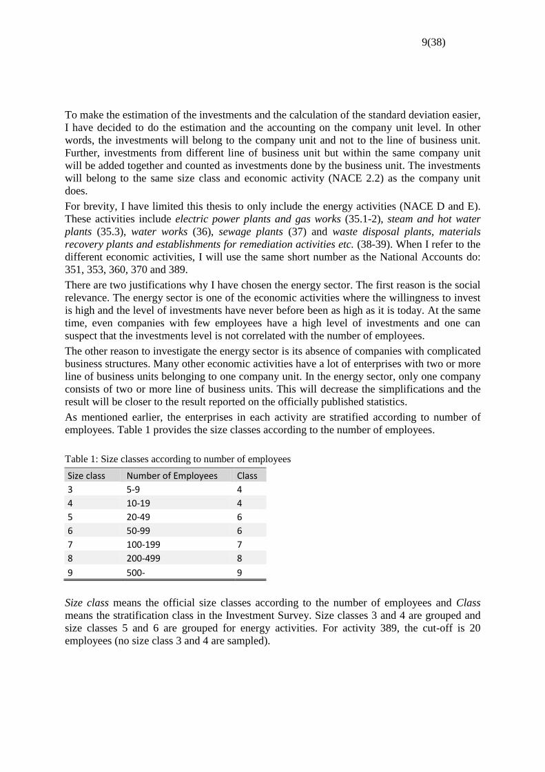
As mentioned earlier, the enterprises in each activity are stratified according to number of

employees. Table 1 provides the size classes according to the number of employees.

Table 1: Size classes according to number of employees

Size class Number of Employees Class

3 5-9 4

4 10-19 4

5 20-49 6

6 50-99 6

7 100-199 7

8 200-499 8

9 500- 9

Size class means the official size classes according to the number of employees and Class

means the stratification class in the Investment Survey. Size classes 3 and 4 are grouped and

size classes 5 and 6 are grouped for energy activities. For activity 389, the cut-off is 20

employees (no size class 3 and 4 are sampled).

10(38)

*

To simplify and since I predict a whole population, I will pretend that all enterprises has

responded to the survey. Further, I will not adjust the formally allocated stratum sample size.

In other words, even if a sample includes all enterprises in a stratum except for one, I will not

change the size of the sample. And finally, no enterprises will be picked in extra and no

enterprises will be coded as outliers.

I have chosen to investigate the investments done in year 2011, which is the latest year where

there are results for. In other words, the sample and the frame are from March 2011 and the

result is collected in February 2012.

1.5 Structure of the Thesis

After the introduction in this chapter, I will discuss the methods used in the thesis in the next

chapter. In chapter three, the results are presented. The chapter starts with a discussion about

the choice of stratification variable. Then, I will discuss the prediction of the investments in

the frame and some statistics. After that, I will discuss the result and some statistics from the

sampling and allocation. And in the end of the chapter, I will discuss the estimator and their

standard deviations.

In the last chapter, I will discuss the result and draw some conclusions.

11(38)

*

2. Methods used in this Thesis

2.1 Choose of the new Variable

When choosing the new variable(s), I have to find the variable with the strongest relationship

with investments. In other words, I have to find the variable with the best fit and the variable

that minimize the sum of the squared vertical distances between the observed independent

variables and the independent variables estimated in the regression. The method I will use to

find the best fit is the Ordinary Least Squares (OLS) method.

Linear regression is widely used in order to analysis relationships between variables. In many

cases, a linear relationship provides a good model of the process, or at least a good

approximation of the model of the process. Linear regression is also very useful for many

economic and business applications. The equation for simple linear regression is:

(1)

where is the dependent variable (investment), is the intercept, is the slope, is the

independent variable and is the error term, i.e. the variance in the y-variable which could

not be explained by the x-variable, or the difference between the predicted y and the “real” y.

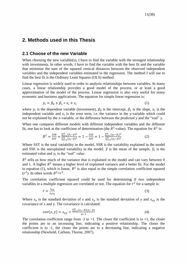
When one compares different models with different independent variables and the different

fit, one has to look at the coefficient of determination (the -value). The equation for is:

∑ ( )

∑ ( )

∑ ( )

∑ ( )

(2)

Where SST is the total variability in the model, SSR is the variability explained in the model

and SSE is the unexplained variability in the model. is the mean of the sample, is the

estimated value and is the “real” value.

tells us how much of the variance that is explained in the model and can vary between 0

and 1. A higher means a higher level of explained variance and a better fit. For the model

in equation (1), which is linear, is also equal to the simple correlation coefficient squared

( ). In other words = .

The correlation coefficient squared could be used for determining if two independent

variables in a multiple regression are correlated or not. The equation for for a sample is:

(3)

Where is the standard deviation of x and is the standard deviation of y and is the

covariance of x and y. The covariance is calculated:

( ) ∑ (

)( )

(4)

The correlation coefficient range from -1 to +1. The closer the coefficient is to +1, the closer

the points are to an increasing line, indicating a positive relationship. The closer the

coefficient is to -1, the closer the points are to a decreasing line, indicating a negative

relationship (Newbold, Carlson, Thorne, 2007).

12(38)

*

2.2 Predication of Investments for the Enterprises Outside the Sample

In this subchapter, I will generate an artificial population. The purpose of the artificial

population is to create investment data for the total population and on basis on this, try

different sampling and allocation strategies.

As mentioned earlier, investments often have a skewed distribution. Some companies invest a

lot, some companies invest less and some companies invest nothing. To manage that, and

made my artificial population as similar as possible as the “real” population, I will draw a

sample of companies whose investments I will set to zero. These companies will be

proportional to the “real” companies which have invested nothing. To calculate the number of

companies with zero investments, I will use the equation:

(5)

where is the number of companies with zero investments in the frame (except from the

companies in the sample), is the number of companies in the sample with zero

investments, N is the number of companies in the frame (except from the companies in the

sample) and n is the number of companies in the sample.

The method I will use when drawing my sample is stratified simple random sample without

replacement (STSRS). The method for STSRS is described in chapter 2.3, where I will

discuss different sample methods.

After drawing the sample of companies whose investments I will set to zero, I will predict the

investments for the rest of the companies in the frame. In order to predict the investments, I

will simply assume that the investments for each company are the mean of the investments in

each stratum.

When using this method, the fit of the model will be too “perfect”. All the predicted values in

one stratum will lie on a line. To manage that, I will take the error terms into consideration.

Therefore, the equation for the model will be:

( ) ( ) (6)

where is the mean value of the investments in each stratum, ( ) is the standard

deviation of the residuals in each stratum and Normal(1) is a standard normally distributed

random seed.

To calculate the standard deviation of the residuals, I will use the equation:

( ) ∑

( ) (7)

where is the difference between the predicted and expected value (residuals or SSE) and

∑ is the sum of squared residuals, n is the number of observations and p is the number of

parameters (Gujarati and Porter, 2009).

Since some of the strata have very low investments and very high error term, I have to ensure

that no investment is negative. To do that, I will expend equation (6) to:

13(38)

*

{ ( ) ( ) { ( ) ( )}

(8)

This may overestimate my population, since some of the investments will get zero investment

instead of negative investment. Since it will just be a few enterprises in some of the strata, I

decided that a small overestimation was preferable compared to manage negative investments.

See Appendix B for SAS-code for the prediction.

2.3 Sampling and Allocation

I will use two types of methods when drawing the sample. The first one is Stratified Simple

Random Sampling without replacement and Neyman allocation, as in the real Investment

Survey. The second type is Probability Proportional to Size without replacement.

2.3.1 Stratified Simple Random Sampling Without Replacement and Neyman Allocation

Simple random sampling (SRS) is widely used when the values of the variables do not vary

much and the population is homogeny. SRS is in many aspects one of the simplest sample

methods and no supplementary information is needed. Further, if a sample is drawn with SRS,

no sample weights are needed when analyzing survey data by, for instance, regression or

multivariate analysis. The disadvantage with SRS is the difficulty to controlling the precision

and the inefficiency of not using supplementary information, which can lead to unnecessary

large samples. Further, there is always a risk of a skewed sample, since supplementary

information is not used (Statistics Sweden, 2008).

In stratified simple random sampling (STSRS4), the frame is divided into different strata.

Within each stratum, each sample is drawn by SRS. Every sample s of the size n in a stratum

has the same probability to be selected. Further, the size n is fixed and the sample is drawn

without replacement. The probability to draw a sample s in one stratum is:

( ) {

( )⁄

(9)

where p(s) is the probability of being in the sample, N is the number of companies in the

frame and n is the number of companies drawn in one stratum. The inclusion probability is:

( )

( )

Where ⁄ is called the sampling fraction. If k=1,..., N, the first-order inclusion

probabilities are all equal to (Särndal, Swensson and Wretman, 1992).

4 In Särndal et al (2002), the term STSI is used instead of STSRS.

14(38)

*

In stratified sampling, the population is divided into non overlapping subpopulations called

strata. In each stratum, a probability sample is selected independently. Stratified sampling has

the advantage that the precision can be specified in each stratum. Further, practical aspects

related to response, measurement and auxiliary information may differ from one

subpopulation to another and this information can improve the efficiency by stratify the

population. For administrative reasons, geographical territories can be used as different

geographical strata.

In stratified sampling, we have a finite population { } which is partitioned

into H subpopulations called strata and denoted where {k : k belongs to

stratum h}. Since the strata form a partition of U, we will have ∑ , whereas is

the number of elements in the stratum h. The total population can be decomposed as:

∑ ∑ ∑

(10)

where ∑ is the total stratum and

is the stratum mean. Then, the estimator of

the population ∑ is:

∑ (11)

where is the estimator of ∑ . Under the STSRS design, the estimator of the

total population ∑ is:

∑

(12)

where ∑

⁄

. Then, the sampling fraction will be expressed as ⁄ and the

stratum variance is:

∑ (

)

(13)

where ∑ ⁄

(Särndal et al, 1992).

The method I will use for allocation in my sample is Neyman allocation. Neyman allocation is

a special case of optimal allocation and is used when the costs in the strata are equal and the

variances in the strata are unequal. If the variances in the strata are, in fact, equal, proportional

allocation is probably the best allocation to use. In cases when the variances vary, optimal

allocation is preferable, since larger units are likely to be more variable then smaller units.

When using proportional allocation, larger units would not be sampled in a higher proportion

and the sample may be biased. For optimal allocation, the equation is:

(

√ ⁄

∑

√ ⁄

) (14)

where n is the total sample size, is the number of units in the population h,

is the

variance of the population in the study variable y in stratum h and is the cost of study an

object in stratum h. Since the variance of the population often is unknown, the variance of the

sample is often used instead.

15(38)

*

In other words, the sample size n in stratum h is proportional to the stratum size multiplied by

the standard deviation of the stratum and divided by the square root of the cost. If the costs are

(approximately) equal for all study units, one can use Neyman allocation and the equation will

be reduced to:

(

∑

) (15)

In Neyman allocation, the total sample size is proportional to the stratum size multiplied by

the standard deviation of the stratum. If the variances are specified correctly, Neyman

allocation will give an estimator with smaller variance compared to proportional allocation

(Lohr, 2010).

Neyman allocation (and optimal allocation) is only optimal for HT-estimation. For GREG-

estimation, the same equation can be used, but with replaced by , the population

standard deviation of the residuals . Since the population standard deviation of the residuals

often is unknown, the sample standard deviation of the residuals is often used instead

(Statistics Sweden, 2008).

Using instead of is optimal for GREG-estimation, in terms of small variances. To

simplify the allocation, and avoid doing double allocation, I have decided to use for my

GREG-estimations as well. In reality, is often replaced by .

2.3.2 Probability Proportional to Size Without Replacement

The second method I will use when drawing my sample is Probability Proportional to Size

without replacement ( 5). The advantage with is that we do not have to care about the

allocation. Further, we do not have to divide the population into different strata (size classes).

In -sampling, the inclusion probability should satisfy where , ,… are

known and positive numbers. The first-order inclusion probabilities (for k=1,…, N) should

be proportional to x and the second order inclusion probabilities should satisfy >0 for all

. Further, the actual selection of the sample can be relatively simple and can be

calculated easily. The difference (for all k≠l) guarantees that the Sen-

Yates-Grundy variance estimator always is positive (for more details about the Sen-Yates-

Grundy variance, see Särndal et al 1992).

There are many different kinds of PPS or methods. The method used in SAS (and the

method I will use) is the Hanurav-Vijayan algorithm for PPS selection without replacement.

When using this method, one can calculate the join selection probabilities. The values of the

joint selection probabilities usually ensure that the Sen-Yates-Grundy variance estimator is

positive and stable (SAS User’s Guide).

5 Normally, the method is named PPS when the sample is drawn with replacement and when the sample is

drawn without replacement. In SAS Users Guide, the method is named PPS, but the sample is drawn without

replacement. I will use the method when the sample is drawn without replacement ( in Särndal et al, but PPS

in SAS). In order not to confuse the readers to much, I will only discuss sampling without replacement in this

thesis.

16(38)

*

In this method, all the units in the stratum is ordered in descending order by size measure6 and

k=1,…, N index the elements. k=1 corresponds to the element with the largest x-value and

k=N correspond to the element with the smallest x-value.

When k=1, I will generate a Unif(0,1) random number and then calculate the probability

using the equation:

∑

(16)

If , I will select the element k=1. Otherwise, I will not.

In next step, I will define a “reduced population” U={k, k+1, …,N, for k=2, 3…N, generate an

independent Unif (0,l) and calculate the new probability using the equation:

( )

(17)

where ∑ and is the number of elements selected

among the first k-1 elements in the population in the first step. If , I will select the

element k. Otherwise, I will not.

The process will continue until or , where { }, with

is equal to the smallest k for which ⁄ .

If the process stop when <n, the process has not produced the full sample size n. In this

case, the final elements are selected from the remaining elements by the

SRS design (see Ch. 2.3.1). That means that for each element, , , I will

generate an independent Unif(1,0) random number and calculate using the equation:

(18)

If < , the element k is selected, otherwise not. The process ends when .

The first order inclusion probability can be calculated using the equation:

{ ⁄

⁄

(19)

where ( ⁄ ). This method only leads to a strict -sampling if the

smallest elements have the same -value. If the smallest elements do not have

the same -value, one can smooth out the for the last elements (Särndal et al,

1992).

Since the relative size of each sampling unit cannot exceed (1/n) and the number of units

sampled by certain cannot exceed the specified sample size, I have to start the sampling

procedure by calculating the cut-off value for the units sampled by certain in each activity

(SAS User’s Guide). The inclusion probability is calculated by:

∑

(20)

6 In my example, the companies’ number of employees or turnover.

17(38)

*

where is a measure of size for unit k=1, 2,..., N and n is the sample size and

(Statistics Sweden). Just as before, all the units in the stratum is ordered in descending order

by size measure and k=1,…, N index the elements. k=1 corresponds to the element with the

largest x-value and k=N correspond to the element with the smallest x-value. Then I will

sample the first element by certain and calculate the new inclusion probability for the rest of

the elements, using the formula:

( )

∑ ( )

(21)

where c is the number of elements sampled by certain. This process will continue until all the

units left has an inclusion probability <1. The x-value of the latest element sampled by certain

is the cut-off value.7

2.4 Estimation

When analysing the quality in the estimated values, there are two approaches one can adopt:

the model-based and the design-based. In the model-based approach the relation between

and is described by a stochastic approach and holds for every observation in the population.

If the observations in the population really follow the model (which it rarely does) and the

inclusion probability depends on y only through the x:s, the sample design should have no

effect. Only one sample is needed and Ordinary Least Squares is used to find the model that

generates the estimate of the population. On the other hand, in the design-based approach, the

finite population characteristics are of interest and the issue of how well the model fits the

population is less important. The random variables define the probability structure used for

inference and indicate inclusion in the sample. Repeated samplings from the finite populations

base the inference. The analysis of the data does not rely on any theoretical model, since we

do not necessarily know the model (Lohr, 2010).

2.4.1 Horvitz-Thompson Estimate and Variance

In Horvitz-Thompson Estimation (HT), the total value is estimated by the sum of the products

of the observed values for the sampled units and the units’ weights. The estimated values will

on average correspond to the values of the total population. The advantage of HT is the

accuracy of the estimation and HT-estimation is sometimes used as reference estimation. The

disadvantage is that HT is not the most efficient estimation. In other words, the variance for

an HT-estimation is sometimes unnecessary big. To decrease the variance without increasing

the sample, one can use auxiliary information, post-stratification or generalized regression

estimation, GREG (Statistics Sweden, 2008).

In a sample (without replacement), the inclusion probability is ( )

and the joint inclusion probability is ( ). can

be calculated as the sum of the probabilities of all samples containing the i:th units. The

property for that is:

7 This formula is a development of earlier formulas. I did not find any reference for it and therefore, I just

explained how to calculate it.

18(38)

*

∑ (22)

where is the inclusion probability for each unit, n is the sample and N is the Frame. For

the property is calculated as:

∑ ( )

(23)

Since the inclusion probability sum up to n, ⁄ is the average probability that a unit will be

selected in one of the draws. Since the units are drawn without replacement, the probability of

selection depends on how many units that was drawn before. Therefore, we will divide the

total t with the average probability ⁄ , when we estimate. From this, the Horvitz-Thompson

estimate can be developed as:

∑

∑

(24)

where if unit i is in the sample and otherwiese. The variance for HT-estimation

is:

( ) ∑

∑ ∑

(25)

When the inclusion probability ( ) and the join inclusion probability ( ) is unequal, the

variance is calculated as:

( ) ∑ ( )

∑ ∑

(26)

To calculate the standard deviation, one has to take the squared root of the variance. (Lohr,

2010).

2.4.2 Generalised Regression estimate and Variance

As mentioned earlier, Generalised Regression Estimation (GREG) and auxiliary information

can be used to reduce the variance of the estimate. One way of using auxiliary information is

doing a ratio estimation. When doing ratio estimation, we will assume that the population we

will estimate is proportional to the auxiliary information and that:

(27)

where is the auxiliary variable and is the variable of interest, ∑ is the total of

the auxiliary variable, ∑ is the total variable of interest, is the mean value for

the auxiliary variable and is the mean value for the variable on interest. B is the ratio for

total auxiliary variable divided by total variable of interest (Lohr 2002). The total of the

variable of interest can in the settings of STSRS be estimated as:

(28)

and

( ) (29)

19(38)

*

Generalised regression estimation (GREG) and auxiliary information can be used to reduce

the mean squared error of the estimate ∑ through the working model:

| (30)

where and ( )

for known. The vector of the true population

totals assumes to be known and is used to adjust the estimator . Then, the generalized

regression estimator of the total population is:

( ) (31)

where B is the weighted least squares estimate of for observations in the population. The

term ( ) is a regression adjustment to the HT-estimator. B is estimated as:

(∑

)

∑

(32)

where is the weighted sum of and can be written as:

∑ (33)

where

( ) (∑

)

(34)

where are the adjustments to the weights. For large samples, we expect to be close to

and then will be close to 1 for many observations. The GREG-estimator will calibrate the

sample to the total population for each x in the regression.

The equation for the variance for a GREG-estimate is:

( ) [ ( ) ] [

] (35)

In a good model, the GREG-estimator will be more efficient than a HT-estimator and the

variability in the residuals will be smaller. For instance, the equation for the variance for a

GREG-estimator in an SRS is:

( )

(

)

∑

(36)

where and is the i:th residual. For Ratio estimation, the working model is:

(37)

and

( ) (38)

The quantity of the population B is the weighted least squares estimate of using the whole

population. The calculation for the ratio is done by equation (32), which gives us:

(∑

)

∑

∑

∑

(39)

and by substitute equation (39) into equation (29), we are back in equation (28), which is the

GREG-estimator of the total population (Lohr, 2010).

20(38)

*

3. Results

All the analyses in this thesis are done with the software SAS 9.2. The procedures used are:

Proc Reg for calculating the -value and Proc Corr for the correlation coefficient. Proc

Surveyselect is used for sampling the enterprises with zero investments and Proc Reg is

included in the macro for predicting the artificial population. The variances for the allocation

are calculated by Proc Summary and the samples are drawn by Proc Surveyselect.

3.1 Choose of the New Variable

In order to choose the new stratification variables, I want to choose some variables that have

some correlation with investments. The proposed variables are: turnover, percent change in

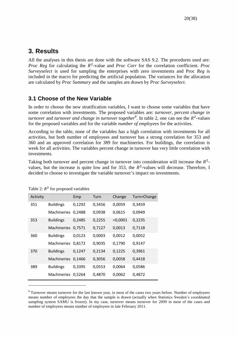
turnover and turnover and change in turnover together8. In table 2, one can see the -values

for the proposed variables and for the variable number of employees for the activities.

According to the table, none of the variables has a high correlation with investments for all

activities, but both number of employees and turnover has a strong correlation for 353 and

360 and an approved correlation for 389 for machineries. For buildings, the correlation is

week for all activities. The variables percent change in turnover has very little correlation with

investments.

Taking both turnover and percent change in turnover into consideration will increase the -

values, but the increase is quite low and for 353, the -values will decrease. Therefore, I

decided to choose to investigate the variable turnover’s impact on investments.

Table 2: for proposed variables

Activity Emp Turn Change Turn+Change

351 Buildings 0,1292 0,3456 0,0059 0,3459

Machineries 0,2488 0,0938 0,0615 0,0949

353 Buildings 0,2485 0,2255 <0,0001 0,2235

Machineries 0,7571 0,7127 0,0013 0,7118

360 Buildings 0,0123 0,0003 0,0012 0,0052

Machineries 0,8172 0,9035 0,1790 0,9147

370 Buildings 0,1247 0,2134 0,1225 0,3961

Machineries 0,1466 0,3056 0,0058 0,4418

389 Buildings 0,3395 0,0553 0,0064 0,0586

Machineries 0,5264 0,4870 0,0062 0,4872

8 Turnover means turnover for the last known year, in most of the cases two years before. Number of employees

means number of employees the day that the sample is drawn (actually when Statistics Sweden’s coordinated

sampling system SAMU is frozen). In my case, turnover means turnover for 2009 in most of the cases and

number of employees means number of employees in late February 2011.

21(38)

*

When we look at the correlation between number of employees and turnover (table 3), we

find that some activities are highly correlated (just as expected). The correlation in activity

360 is really high, and also the correlation in 353. For 370 and 389, the correlations are lower

and the correlation in 351 is quite low. This is not a big surprise, since the activities with high

correlation also were the ones with similar -values. Since we do not have any better

alternative for independent variable, we will choose turnover as the variable to investigate.

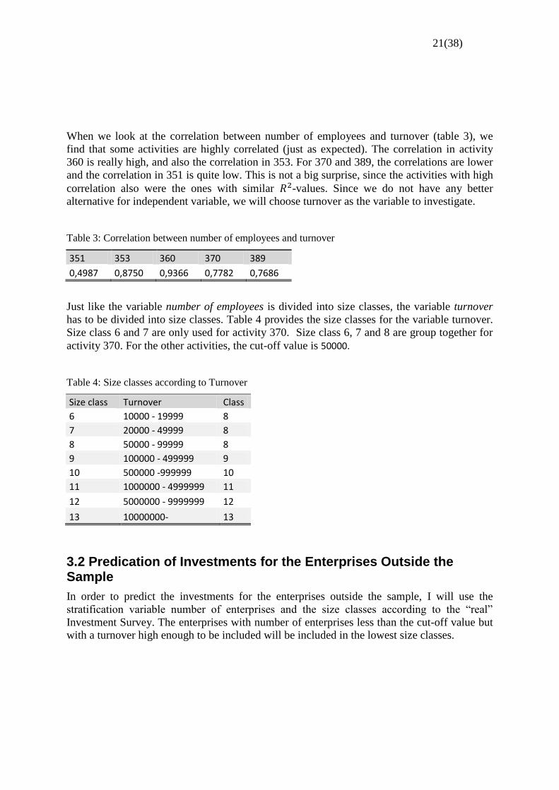
Table 3: Correlation between number of employees and turnover

351 353 360 370 389

0,4987 0,8750 0,9366 0,7782 0,7686

Just like the variable number of employees is divided into size classes, the variable turnover

has to be divided into size classes. Table 4 provides the size classes for the variable turnover.

Size class 6 and 7 are only used for activity 370. Size class 6, 7 and 8 are group together for

activity 370. For the other activities, the cut-off value is 50000.

Table 4: Size classes according to Turnover

Size class Turnover Class

6 10000 - 19999 8

7 20000 - 49999 8

8 50000 - 99999 8

9 100000 - 499999 9

10 500000 -999999 10

11 1000000 - 4999999 11

12 5000000 - 9999999 12

13 10000000- 13

3.2 Predication of Investments for the Enterprises Outside the Sample

In order to predict the investments for the enterprises outside the sample, I will use the

stratification variable number of enterprises and the size classes according to the “real”

Investment Survey. The enterprises with number of enterprises less than the cut-off value but

with a turnover high enough to be included will be included in the lowest size classes.

22(38)

*

I will start the prediction by calculating the enterprises with zero investments. When counting

the number of enterprises with zero investment, I found that 95 enterprises have zero

investments in buildings and 25 have zero investments in machineries. I will use equation (5)

to calculate the number of enterprises outside the sample with zero investments. The result is

223 enterprises with zero investments in buildings and 75 enterprises with zero investments in

machineries.9

The method for predicting the investment is not a perfect one; however, it is the best one we

have now. More preferable might have been to use simple linear regression. Due to the low

correlation between number of employees and investment, in many strata, linear regression

gave negative intercept or negative slope, resulting in too many negative investments.

The size of the stratum is another issue, since many strata only have a few observations. Since

I had to keep some kind of relationship between size and investment, I had to keep the small

stratum instead of merge size classes. Some of the strata will be without values. This is

because we already have values for all enterprises in the stratum or because the rest of the

enterprises are selected as having zero investment.

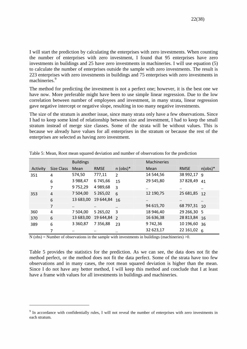
Table 5: Mean, Root mean squared deviation and number of observations for the prediction

Buildings

Machineries

Activity Size Class Mean RMSE n (obs)* Mean RMSE n(obs)*

351 4 574,50 777,11 2

14 544,56 38 992,17 9

6 3 988,47 6 745,66 15

29 545,80 37 828,49 41

7 9 752,29 4 989,68 3

.. .. ..

353 4 7 504,00 5 265,02 6 12 190,75 25 681,85 12

6 13 683,00 19 644,84 16 .. .. ..

7 .. .. .. 94 615,70 68 797,31 10 360 4 7 504,00 5 265,02 3

18 946,40 29 266,30 5

370 6 13 683,00 19 644,84 2 16 636,38 28 813,84 16

389 6 3 360,87 7 356,88 23

9 742,36 10 196,60 36

7 .. .. .. 32 623,17 22 161,02 6

N (obs) = Number of observations in the sample with investments in buildings (machineries) >0.

Table 5 provides the statistics for the prediction. As we can see, the data does not fit the

method perfect, or the method does not fit the data perfect. Some of the strata have too few

observations and in many cases, the root mean squared deviation is higher than the mean.

Since I do not have any better method, I will keep this method and conclude that I at least

have a frame with values for all investments in buildings and machineries.

9 In accordance with confidentially rules, I will not reveal the number of enterprises with zero investments in

each stratum.

23(38)

*

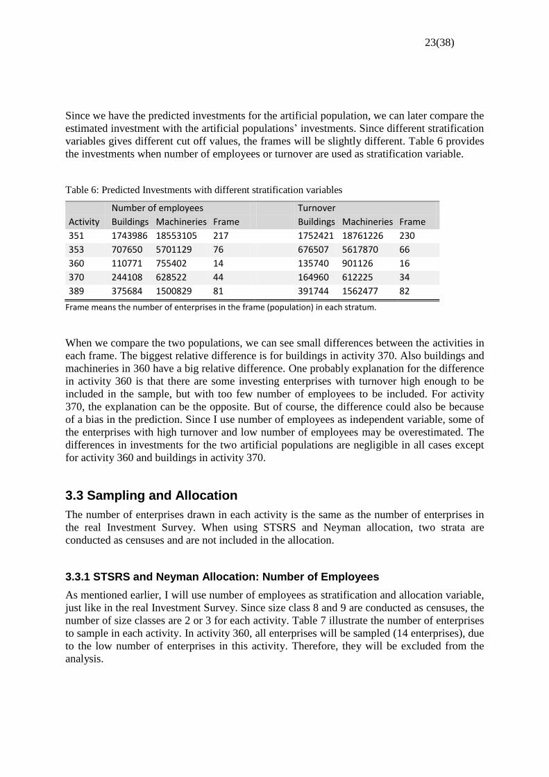
Since we have the predicted investments for the artificial population, we can later compare the

estimated investment with the artificial populations’ investments. Since different stratification

variables gives different cut off values, the frames will be slightly different. Table 6 provides

the investments when number of employees or turnover are used as stratification variable.

Table 6: Predicted Investments with different stratification variables

Number of employees Turnover

Activity Buildings Machineries Frame Buildings Machineries Frame

351 1743986 18553105 217 1752421 18761226 230

353 707650 5701129 76 676507 5617870 66

360 110771 755402 14 135740 901126 16

370 244108 628522 44 164960 612225 34

389 375684 1500829 81 391744 1562477 82

Frame means the number of enterprises in the frame (population) in each stratum.

When we compare the two populations, we can see small differences between the activities in

each frame. The biggest relative difference is for buildings in activity 370. Also buildings and

machineries in 360 have a big relative difference. One probably explanation for the difference

in activity 360 is that there are some investing enterprises with turnover high enough to be

included in the sample, but with too few number of employees to be included. For activity

370, the explanation can be the opposite. But of course, the difference could also be because

of a bias in the prediction. Since I use number of employees as independent variable, some of

the enterprises with high turnover and low number of employees may be overestimated. The

differences in investments for the two artificial populations are negligible in all cases except

for activity 360 and buildings in activity 370.

3.3 Sampling and Allocation

The number of enterprises drawn in each activity is the same as the number of enterprises in

the real Investment Survey. When using STSRS and Neyman allocation, two strata are

conducted as censuses and are not included in the allocation.

3.3.1 STSRS and Neyman Allocation: Number of Employees

As mentioned earlier, I will use number of employees as stratification and allocation variable,

just like in the real Investment Survey. Since size class 8 and 9 are conducted as censuses, the

number of size classes are 2 or 3 for each activity. Table 7 illustrate the number of enterprises

to sample in each activity. In activity 360, all enterprises will be sampled (14 enterprises), due

to the low number of enterprises in this activity. Therefore, they will be excluded from the

analysis.

24(38)

*

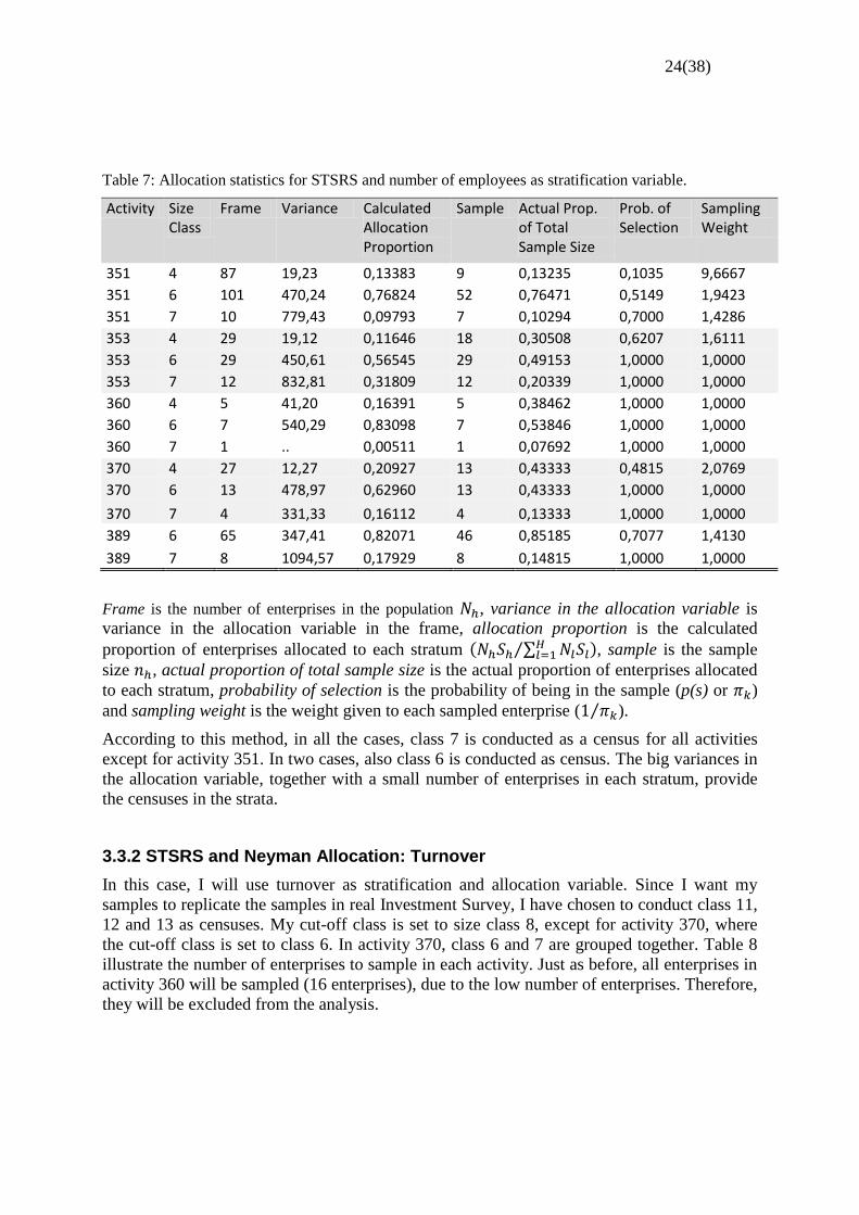
Table 7: Allocation statistics for STSRS and number of employees as stratification variable.

Activity Size Class

Frame Variance Calculated Allocation Proportion

Sample Actual Prop. of Total Sample Size

Prob. of Selection

Sampling Weight

351 4 87 19,23 0,13383 9 0,13235 0,1035 9,6667

351 6 101 470,24 0,76824 52 0,76471 0,5149 1,9423

351 7 10 779,43 0,09793 7 0,10294 0,7000 1,4286

353 4 29 19,12 0,11646 18 0,30508 0,6207 1,6111

353 6 29 450,61 0,56545 29 0,49153 1,0000 1,0000

353 7 12 832,81 0,31809 12 0,20339 1,0000 1,0000

360 4 5 41,20 0,16391 5 0,38462 1,0000 1,0000

360 6 7 540,29 0,83098 7 0,53846 1,0000 1,0000

360 7 1 .. 0,00511 1 0,07692 1,0000 1,0000

370 4 27 12,27 0,20927 13 0,43333 0,4815 2,0769

370 6 13 478,97 0,62960 13 0,43333 1,0000 1,0000

370 7 4 331,33 0,16112 4 0,13333 1,0000 1,0000

389 6 65 347,41 0,82071 46 0,85185 0,7077 1,4130

389 7 8 1094,57 0,17929 8 0,14815 1,0000 1,0000

Frame is the number of enterprises in the population , variance in the allocation variable is

variance in the allocation variable in the frame, allocation proportion is the calculated

proportion of enterprises allocated to each stratum ( ∑ ⁄ ), sample is the sample

size , actual proportion of total sample size is the actual proportion of enterprises allocated

to each stratum, probability of selection is the probability of being in the sample (p(s) or )

and sampling weight is the weight given to each sampled enterprise ( ⁄ ).

According to this method, in all the cases, class 7 is conducted as a census for all activities

except for activity 351. In two cases, also class 6 is conducted as census. The big variances in

the allocation variable, together with a small number of enterprises in each stratum, provide

the censuses in the strata.

3.3.2 STSRS and Neyman Allocation: Turnover

In this case, I will use turnover as stratification and allocation variable. Since I want my

samples to replicate the samples in real Investment Survey, I have chosen to conduct class 11,

12 and 13 as censuses. My cut-off class is set to size class 8, except for activity 370, where

the cut-off class is set to class 6. In activity 370, class 6 and 7 are grouped together. Table 8

illustrate the number of enterprises to sample in each activity. Just as before, all enterprises in

activity 360 will be sampled (16 enterprises), due to the low number of enterprises. Therefore,

they will be excluded from the analysis.

25(38)

*

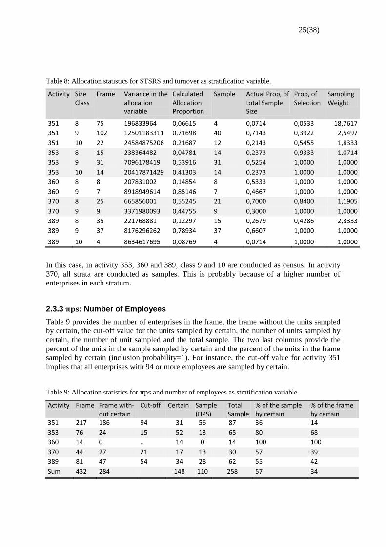
Table 8: Allocation statistics for STSRS and turnover as stratification variable.

Activity Size Class

Frame Variance in the allocation variable

Calculated Allocation Proportion

Sample Actual Prop, of total Sample Size

Prob, of Selection

Sampling Weight

351 8 75 196833964 0,06615 4 0,0714 0,0533 18,7617

351 9 102 12501183311 0,71698 40 0,7143 0,3922 2,5497

351 10 22 24584875206 0,21687 12 0,2143 0,5455 1,8333

353 8 15 238364482 0,04781 14 0,2373 0,9333 1,0714

353 9 31 7096178419 0,53916 31 0,5254 1,0000 1,0000

353 10 14 20417871429 0,41303 14 0,2373 1,0000 1,0000

360 8 8 207831002 0,14854 8 0,5333 1,0000 1,0000

360 9 7 8918949614 0,85146 7 0,4667 1,0000 1,0000

370 8 25 665856001 0,55245 21 0,7000 0,8400 1,1905

370 9 9 3371980093 0,44755 9 0,3000 1,0000 1,0000

389 8 35 221768881 0,12297 15 0,2679 0,4286 2,3333

389 9 37 8176296262 0,78934 37 0,6607 1,0000 1,0000

389 10 4 8634617695 0,08769 4 0,0714 1,0000 1,0000

In this case, in activity 353, 360 and 389, class 9 and 10 are conducted as census. In activity

370, all strata are conducted as samples. This is probably because of a higher number of

enterprises in each stratum.

2.3.3 : Number of Employees

Table 9 provides the number of enterprises in the frame, the frame without the units sampled

by certain, the cut-off value for the units sampled by certain, the number of units sampled by

certain, the number of unit sampled and the total sample. The two last columns provide the

percent of the units in the sample sampled by certain and the percent of the units in the frame

sampled by certain (inclusion probability=1). For instance, the cut-off value for activity 351

implies that all enterprises with 94 or more employees are sampled by certain.

Table 9: Allocation statistics for and number of employees as stratification variable

Activity Frame Frame with-out certain

Cut-off Certain Sample (ПPS)

Total Sample

% of the sample by certain

% of the frame by certain

351 217 186 94 31 56 87 36 14

353 76 24 15 52 13 65 80 68

360 14 0 .. 14 0 14 100 100

370 44 27 21 17 13 30 57 39

389 81 47 54 34 28 62 55 42

Sum 432 284 148 110 258 57 34

26(38)

*

Since -sample uses number of employees as allocation variable, a high spread of number

of enterprises in an activity will result in a high number of enterprises sampled by certain. In

activity 370 and 389, more than half of the enterprises sampled are sampled by certain. In

activity 351, almost two third of the sampled enterprises are sampled by certain. In activity

353, almost 80 percent of the sampled enterprises are sampled by certain. The proportion of

the frame sampled by certain varies between 14 and 68 percent (100 percent for activity 360).

432 enterprises are included in the frame, 258 are sampled and 148 are sampled by certain.

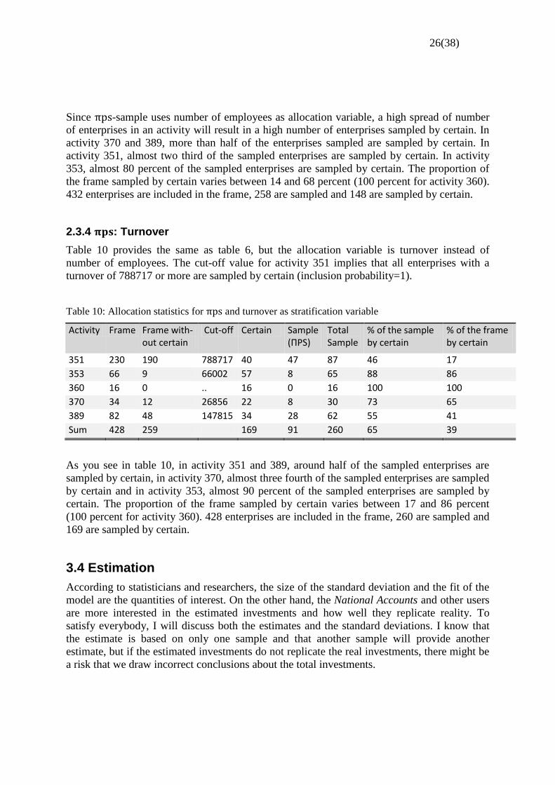
2.3.4 : Turnover

Table 10 provides the same as table 6, but the allocation variable is turnover instead of

number of employees. The cut-off value for activity 351 implies that all enterprises with a

turnover of 788717 or more are sampled by certain (inclusion probability=1).

Table 10: Allocation statistics for and turnover as stratification variable

Activity Frame Frame with-out certain

Cut-off Certain Sample (ПPS)

Total Sample

% of the sample by certain

% of the frame by certain

351 230 190 788717 40 47 87 46 17

353 66 9 66002 57 8 65 88 86

360 16 0 .. 16 0 16 100 100

370 34 12 26856 22 8 30 73 65

389 82 48 147815 34 28 62 55 41

Sum 428 259 169 91 260 65 39

As you see in table 10, in activity 351 and 389, around half of the sampled enterprises are

sampled by certain, in activity 370, almost three fourth of the sampled enterprises are sampled

by certain and in activity 353, almost 90 percent of the sampled enterprises are sampled by

certain. The proportion of the frame sampled by certain varies between 17 and 86 percent

(100 percent for activity 360). 428 enterprises are included in the frame, 260 are sampled and

169 are sampled by certain.

3.4 Estimation

According to statisticians and researchers, the size of the standard deviation and the fit of the

model are the quantities of interest. On the other hand, the National Accounts and other users

are more interested in the estimated investments and how well they replicate reality. To

satisfy everybody, I will discuss both the estimates and the standard deviations. I know that

the estimate is based on only one sample and that another sample will provide another

estimate, but if the estimated investments do not replicate the real investments, there might be

a risk that we draw incorrect conclusions about the total investments.

27(38)

*

The estimation and the calculating of the standard deviations are done with a statistical macro

program for SAS called CLAN 97 v3.1. CLAN is a SAS-program for computation of point

and standard deviation estimate in sample surveys. CLAN is developed for Statistics Sweden

by Claes Andersson and Lennart Nordberg.

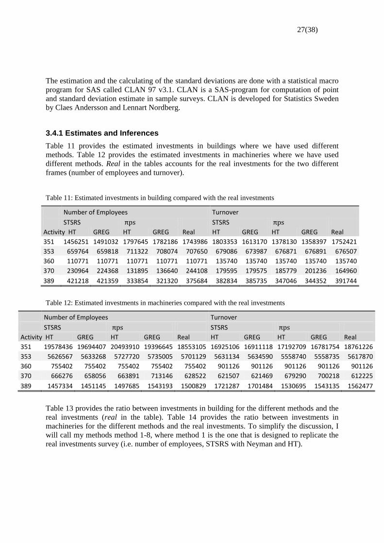
3.4.1 Estimates and Inferences

Table 11 provides the estimated investments in buildings where we have used different

methods. Table 12 provides the estimated investments in machineries where we have used

different methods. Real in the tables accounts for the real investments for the two different

frames (number of employees and turnover).

Table 11: Estimated investments in building compared with the real investments

Number of Employees Turnover

STSRS STSRS

Activity HT GREG HT GREG Real HT GREG HT GREG Real

351 1456251 1491032 1797645 1782186 1743986 1803353 1613170 1378130 1358397 1752421

353 659764 659818 711322 708074 707650 679086 673987 676871 676891 676507

360 110771 110771 110771 110771 110771 135740 135740 135740 135740 135740

370 230964 224368 131895 136640 244108 179595 179575 185779 201236 164960

389 421218 421359 333854 321320 375684 382834 385735 347046 344352 391744

Table 12: Estimated investments in machineries compared with the real investments

Number of Employees Turnover

STSRS STSRS

Activity HT GREG HT GREG Real HT GREG HT GREG Real

351 19578436 19694407 20493910 19396645 18553105 16925106 16911118 17192709 16781754 18761226

353 5626567 5633268 5727720 5735005 5701129 5631134 5634590 5558740 5558735 5617870

360 755402 755402 755402 755402 755402 901126 901126 901126 901126 901126

370 666276 658056 663891 713146 628522 621507 621469 679290 700218 612225

389 1457334 1451145 1497685 1543193 1500829 1721287 1701484 1530695 1543135 1562477

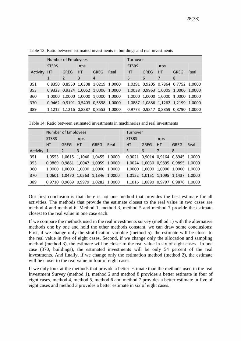
Table 13 provides the ratio between investments in building for the different methods and the

real investments (real in the table). Table 14 provides the ratio between investments in

machineries for the different methods and the real investments. To simplify the discussion, I

will call my methods method 1-8, where method 1 is the one that is designed to replicate the

real investments survey (i.e. number of employees, STSRS with Neyman and HT).

28(38)

*

Table 13: Ratio between estimated investments in buildings and real investments

Number of Employees Turnover

STSRS STSRS

Activity HT GREG HT GREG Real HT GREG HT GREG Real

1 2 3 4 5 6 7 8

351 0,8350 0,8550 1,0308 1,0219 1,0000

1,0291 0,9205 0,7864 0,7752 1,0000

353 0,9323 0,9324 1,0052 1,0006 1,0000 1,0038 0,9963 1,0005 1,0006 1,0000

360 1,0000 1,0000 1,0000 1,0000 1,0000

1,0000 1,0000 1,0000 1,0000 1,0000

370 0,9462 0,9191 0,5403 0,5598 1,0000 1,0887 1,0886 1,1262 1,2199 1,0000

389 1,1212 1,1216 0,8887 0,8553 1,0000 0,9773 0,9847 0,8859 0,8790 1,0000

Table 14: Ratio between estimated investments in machineries and real investments

Number of Employees Turnover

STSRS STSRS

HT GREG HT GREG Real HT GREG HT GREG Real

Activity 1 2 3 4 5 6 7 8

351 1,0553 1,0615 1,1046 1,0455 1,0000

0,9021 0,9014 0,9164 0,8945 1,0000

353 0,9869 0,9881 1,0047 1,0059 1,0000 1,0024 1,0030 0,9895 0,9895 1,0000

360 1,0000 1,0000 1,0000 1,0000 1,0000

1,0000 1,0000 1,0000 1,0000 1,0000

370 1,0601 1,0470 1,0563 1,1346 1,0000 1,0152 1,0151 1,1095 1,1437 1,0000

389 0,9710 0,9669 0,9979 1,0282 1,0000 1,1016 1,0890 0,9797 0,9876 1,0000

Our first conclusion is that there is not one method that provides the best estimate for all

activities. The methods that provide the estimate closest to the real value in two cases are

method 4 and method 6. Method 1, method 3, method 5 and method 7 provide the estimate

closest to the real value in one case each.

If we compare the methods used in the real investments survey (method 1) with the alternative

methods one by one and hold the other methods constant, we can draw some conclusions:

First, if we change only the stratification variable (method 5), the estimate will be closer to

the real value in five of eight cases. Second, if we change only the allocation and sampling

method (method 3), the estimate will be closer to the real value in six of eight cases. In one

case (370, buildings), the estimated investments will be only 54 percent of the real

investments. And finally, if we change only the estimation method (method 2), the estimate

will be closer to the real value in four of eight cases.

If we only look at the methods that provide a better estimate than the methods used in the real

Investment Survey (method 1), method 2 and method 8 provides a better estimate in four of

eight cases, method 4, method 5, method 6 and method 7 provides a better estimate in five of

eight cases and method 3 provides a better estimate in six of eight cases.

29(38)

*

So, which method provides the best estimate closest to the real value? According to these

samples, method 3 will decrease the difference between the estimated investment and the real

investment in six of four cases, but for one of the two other cases, the result is far from

satisfactory. How should we handle that? Since the population in 370 is quite small, only 44

enterprises, and we sample 40 enterprises, a possibly solution may be that we decide to

conduct the whole activity as a census. Then, keep the same stratification variable and

estimation method, but change the sampling method to will be an acceptable method for

both estimations in buildings and machineries. But before we draw any conclusions, we have

to look at the standard deviations for the estimators.

3.4.2 Standard Deviations

In this chapter, I will discuss the different standard deviations for the different methods and

draw some conclusions about the size of the standard deviation and the precision of the

estimations. Since the populations and the total investments are a bit different for different

allocation variables, one has to take that into consideration when analysing the standard

deviation, since some of the differences in size can derive from that. In most of the cases, we

can ignore that, since the difference is small, but for buildings in activity 370, the difference is

almost one third of the investments and therefore, we have to consider that.

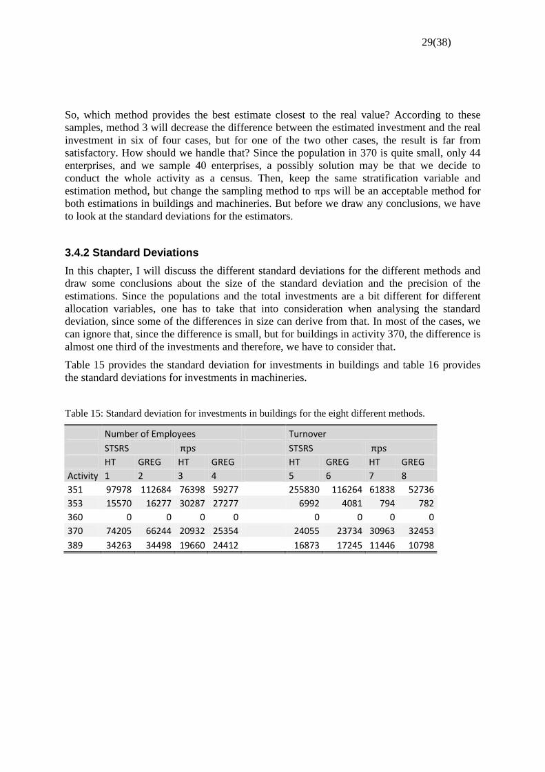
Table 15 provides the standard deviation for investments in buildings and table 16 provides

the standard deviations for investments in machineries.

Table 15: Standard deviation for investments in buildings for the eight different methods.

Number of Employees Turnover

STSRS STSRS

HT GREG HT GREG HT GREG HT GREG

Activity 1 2 3 4 5 6 7 8

351 97978 112684 76398 59277

255830 116264 61838 52736

353 15570 16277 30287 27277 6992 4081 794 782

360 0 0 0 0

0 0 0 0

370 74205 66244 20932 25354 24055 23734 30963 32453

389 34263 34498 19660 24412 16873 17245 11446 10798

30(38)

*

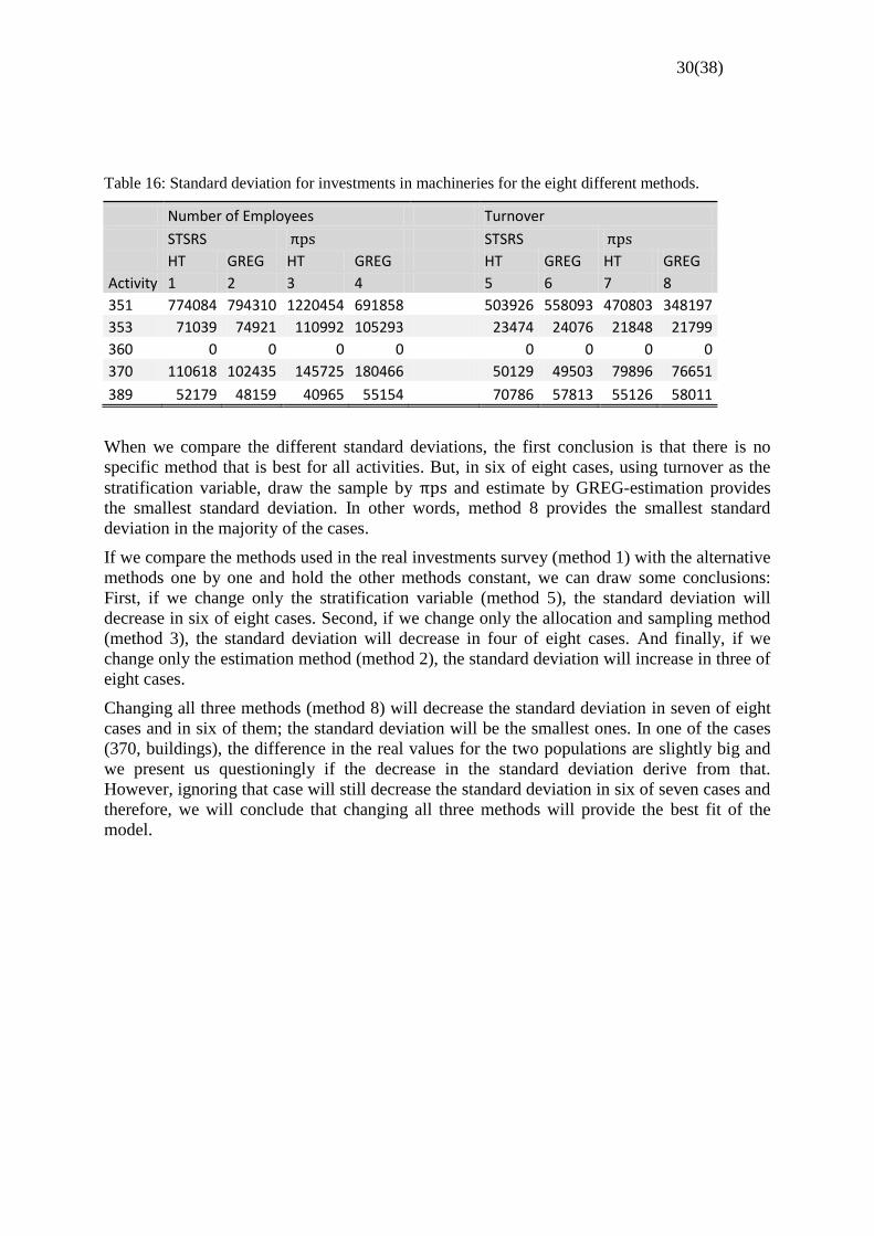
Table 16: Standard deviation for investments in machineries for the eight different methods.

Number of Employees Turnover

STSRS STSRS

HT GREG HT GREG HT GREG HT GREG

Activity 1 2 3 4 5 6 7 8

351 774084 794310 1220454 691858

503926 558093 470803 348197

353 71039 74921 110992 105293 23474 24076 21848 21799

360 0 0 0 0

0 0 0 0

370 110618 102435 145725 180466 50129 49503 79896 76651

389 52179 48159 40965 55154 70786 57813 55126 58011

When we compare the different standard deviations, the first conclusion is that there is no

specific method that is best for all activities. But, in six of eight cases, using turnover as the

stratification variable, draw the sample by and estimate by GREG-estimation provides

the smallest standard deviation. In other words, method 8 provides the smallest standard

deviation in the majority of the cases.

If we compare the methods used in the real investments survey (method 1) with the alternative

methods one by one and hold the other methods constant, we can draw some conclusions:

First, if we change only the stratification variable (method 5), the standard deviation will

decrease in six of eight cases. Second, if we change only the allocation and sampling method

(method 3), the standard deviation will decrease in four of eight cases. And finally, if we

change only the estimation method (method 2), the standard deviation will increase in three of

eight cases.

Changing all three methods (method 8) will decrease the standard deviation in seven of eight

cases and in six of them; the standard deviation will be the smallest ones. In one of the cases

(370, buildings), the difference in the real values for the two populations are slightly big and

we present us questioningly if the decrease in the standard deviation derive from that.

However, ignoring that case will still decrease the standard deviation in six of seven cases and

therefore, we will conclude that changing all three methods will provide the best fit of the

model.

31(38)

*

4. Discussion and Conclusion

In this chapter, I will discuss the result and draw some conclusions. Since we only have

investigated the activities in the energy sector, we cannot draw the conclusions that the result

in this thesis will be applicable to all activities in the Investment Survey. To do that, we need

to elaborate and expand this study to include all activities.

When comparing the conclusion from the estimate and the standard deviation, we find that

they contradict each other. The method that gave the estimates closest to the real values was

stratify on number of employees, sample by and estimate by HG-estimation (method 3).

On the other hand, the method that provided the least standard deviation was stratify on

turnover, sample by and estimate by GREG-estimation (method 8). If we look at the

standard deviations for method 3, the standard deviations are in half of the cases worse than

the real method (method 1). On the other hand, method 8 provides estimates that are worse

than the estimates in the real method in all cases except one. So which method should we

choose the get the best estimates closest to the real values, and at the same time, get the least

standard deviations and the best fit of the model?

Actually, it is not surprising that the two methods contradict each other. When doing -

sampling, the units with a high value on the independent variable (number of employees or

turnover) will get a higher inclusion probability and vice versa for low value on the

independent variable. If a unit has a low value on the independent variable and a high value

on the dependent variable, the inclusion probability will be low and it is most likely that the

unit will not be sampled. The result will be an underestimated estimate, but the standard

deviation will be small, since the sample will be homogenous and the dependent and

independent variables will get a better correlation. If the unit will be sampled, the low

inclusion probability will provide high weights and the estimate will be overestimated. In this

case, the standard deviation will probably be big, since the value of the dependent variable

will be higher than expected.

On the other hand, a unit with a high value on the independent variable and a low value on the

dependent variable will have a high inclusion probability. The unit will probably be in the

sample and the high inclusion probability will provide a low weight for the unit. Since the

value of the dependent variable is lower than expected, the standard deviation will be high

and the estimate will be underestimated. If the unit is not sampled, the units in the sample will

probably be overestimated, but the standard deviation will be low, since the sample will be

homogenous and the dependent and independent variables will be better correlated.

In a population, there will probably be both units with unexpected high values, units with

unexpected low values and units with expected values on the dependent variable. If they are

combined, the over- and underestimated values can, just by chance, cancel out each other and

the estimated value will be close to the real value. In this case, the standard deviation will be

big, even if the estimated value is close to the real value.

Since method 3 and method 8 use different stratification variables, there is not a surprise that

there are different enterprises in different samples. And since the inclusion probabilities of the

enterprises and their weights are based on the stratification variables, there is not a surprise

that both the estimates and the standard deviations are different.

32(38)

*

According to my result in chapter 3.1, there was no dependent variable with a superior better

-value for all activities. And just as expected, there was no obvious winner between stratify

on number of employees or stratify on turnover. But, when comparing all the different

methods with different stratification variables (method 1 with method 5, method 2 with

method 6 and so on), on average, the standard deviation is smaller in 24 of 32 cases when we

stratify on turnover. Turnover may be a register variable, but according to my result, at least

sufficient up-to-date to improve the efficiency in the survey. On this basis, I will conclude that

turnover is a better variable to stratify on.

As mentioned in chapter 1.2 and chapter 2.4.2, generalised regression estimation (GREG) and

auxiliary information can be used to reduce the standard deviation of the estimate, assuming

that the auxiliary information and the dependent variable is correlated. If we compare all the

different methods with different estimators (method 1 with method 2, method 3 with method 4

and so on), we will find that in the majority of the cases (18 of 32), GREG-estimation will

provide a lower standard deviation. On the basis on this, we can conclude that GREG-

estimation is better than HT-estimation. If we also take the stratify variable into consideration,

we will find that changing the estimation method from HT-estimation to GREG-estimation

will provide a lower standard deviation in 11 cases when we stratify on turnover, but only in 7

cases when we stratify on number of employees. This will strengthen our theory that GREG-

estimation and turnover as a stratify variable is a good combination.

In chapter 1.2, I discussed previous research and why many statisticians recommended the

choice of GREG-estimation and auxiliary information instead of HT-estimation when the

sample is drawn by . In my results, if the sample is drawn by , changing from HT-

estimation to GREG-estimation will provide a smaller standard deviation in 10 cases of 16.

Further, if one should do a GREG-estimation, changing sampling method from STSRS to

will provide a smaller standard deviation in 9 cases of 16. From this, we will conclude that

-sampling and GREG-estimations is a good combination in the Investment Survey. If we

also take the stratification variable into consideration, -sampling combined with GREG-

estimation will have a smaller standard deviation in 6 of 8 cases, when turnover is used as

stratification variable instead of number of employees.

As a last comparison: if we compare the standard deviations from the method designed to

replicate the real investments survey (method 1) with the standard deviations from the method

proposed by our result (method 8), the standard deviation will be smaller in 7 of 8 cases (or 6

of 7, if we exclude buildings in 370). From that, we can draw the conclusion that the

combination stratify on turnover, sample by and estimate by GREG-estimation will give

the smallest standard deviation on average and this is also the conclusion in chapter 3.4.2.

But how should we handle the high difference between the estimated values and the real

values? My answer is: the same way as we do today. By picking in a few small enterprises

that we know have big investments with the inclusion probability 1 and coding some of the

small enterprises with high investments as outliers and give them the weight 1. If we do that,

combined with stratify on turnover, sample by and estimate by GREG-estimation, we

will certify both the statisticians and the users and get a result with estimated investments

close to the real investments and with low standard deviations. In other words, we will get the

best design for the Swedish Investment Survey.

33(38)

*

5. References

Djerf, K. (1997) Effects of Post-Stratification on the Estimates of the Finnish Labour Force

Survey, Journal of Official Statistics. Vol. 13, No.1, 1997, pp. 29-39

Estevao, V. M., Särndal, C-E. (2000) A function form approach to calibration, Journal of

Official Statistics. Vol. 16, No.4, 2000, pp. 379-399

Gujarati, D. N., Porter, D. C. (2009) Basic econometrics, fifth edition, International

edition McGraw-Hill/Irwin, New York: McGraw-Hill Higher education.

Hidiroglou, M. A., Patek, Z. (2006) Raking ratio estimation: An application to the Canadian

Retail Trade Survey Journal of Official Statistics. Vol. 22, No.1, 2006, pp. 71-80

Holmberg, A. (2003) Essays on model assisted survey planning, Acta Universitais

Upsaliensis, Comprehensive summaries of Uppsala Dissertations from the Faculty of Social

Sciences 126. Uppsala

Karmel, T.S., Jain, M. (1987) Comparison of purposive and random sampling scheme for

estimation capital expenditure, Journal of the American Statistical Association, Vvol. 83,

Iissue 397 (Mar., 1987) 52-57

Lohr, S. L. (1999) Sampling: design and analysis. 2:nd edition, Pacific Grove: Brooks/Cole

publishing company.

Lu H., Gelman A. (2003) A method for estimating design-based sampling variances for

surveys with weighting, post-stratification and raking, Journal of Official Statistics. Vol. 19,

No.2, 2003, pp. 133-151

Newbold, P., Carlson, W. L., Thorne, B. (2006) Statistics for business and economics. sixth

edition New Jersey: Pearson Prentice Hall. Pearson Education. Inc., Upper Saddle River,

Rosén, B. (2000) Generalized Regression Estimation and Pareto πps, R&D Report 2000:5.

Statistics Sweden.

SAS/STAT(R) 9.2 User's Guide, Second Edition: PPS Sampling without Replacement

34(38)

*

Statistics Sweden. (2008) Urval –från Teori till Praktik SCB-Tryck, Örebro 2008.03.

Statistics Sweden, Research and Development.

Särndahl, C-E., Swensson, B., Wretman, J. (1992) Model assisted survey sampling, New

York: Springer-Verlag.

Thomsen I., Zhang, L.C. (2001) The effects of using administrative registers in economic

short term statistics: The Norwegian Labour Force Survey as a case study, Journal of Official

Statistics. Vol. 17, No.2, 2001, pp. 285-294

Zheng, H., Little, R. J. A. (2003) Penalized spline model-based estimation of the finite

populations total from probability-proportional-to-size samples, Journal of Official Statistics.

Vol. 19, No.2, 2003, pp. 99-107

Zheng, H., Little, R. J. A. (2005) Inference for the population total from probability-

proportional-to-size samples based on predictions from a penalized spline nonparametric

model, Journal of Official Statistics. Vol. 21, No.1, 2005, pp. 1-20

For information about economic activity and NACE 2.2:

http://www.sni2007.scb.se/

For information about the Swedish Investment Survey:

http://www.scb.se/nv0801

http://www.scb.se/nv0801-en

Beskrivning av Statistiken: Näringslivets Investeringar 2011. 2012 NV0801 (BAS). Statistics

Sweden

Näringslivets Investeringar 2011 (SCBDOK), Statistics Sweden

Intern documentation

Produktionshandledning för Investeringsenkäten

Urvalsbeställning 2011

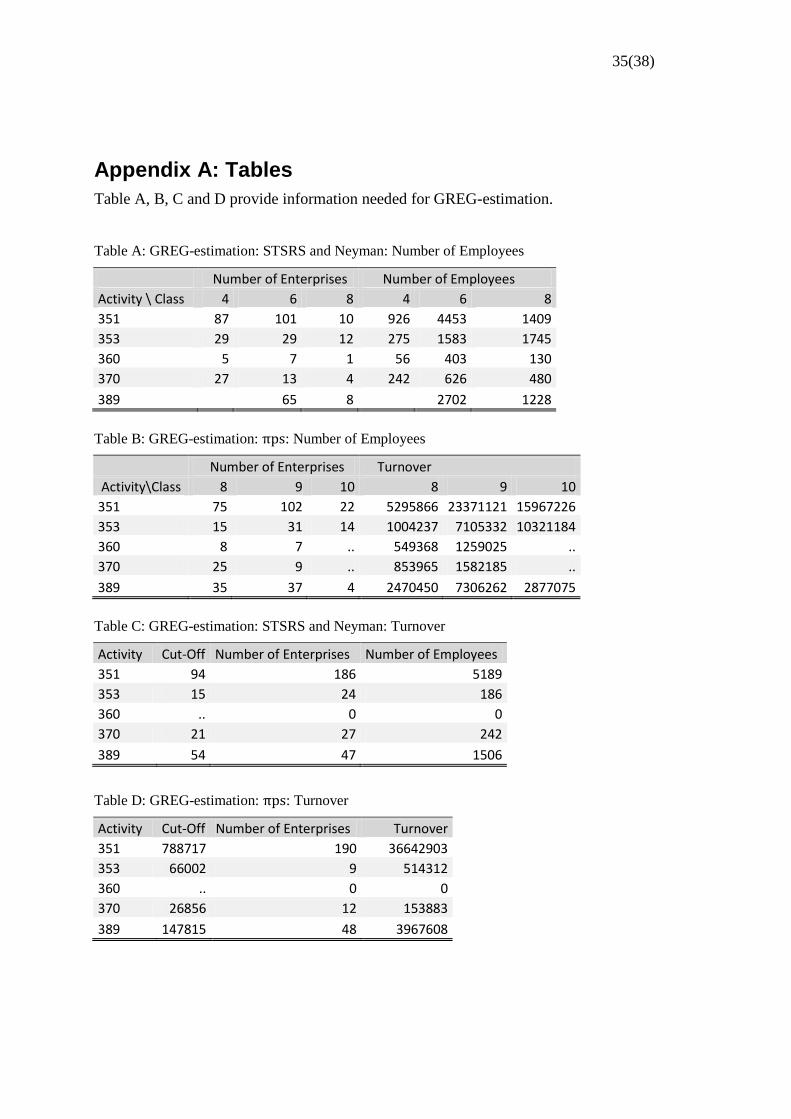
35(38)

*

Appendix A: Tables

Table A, B, C and D provide information needed for GREG-estimation.

Table A: GREG-estimation: STSRS and Neyman: Number of Employees

Number of Enterprises Number of Employees

Activity \ Class 4 6 8 4 6 8

351 87 101 10 926 4453 1409

353 29 29 12 275 1583 1745

360 5 7 1 56 403 130

370 27 13 4 242 626 480

389 65 8 2702 1228

Table B: GREG-estimation: : Number of Employees

Number of Enterprises Turnover

Activity\Class 8 9 10 8 9 10

351 75 102 22 5295866 23371121 15967226

353 15 31 14 1004237 7105332 10321184

360 8 7 .. 549368 1259025 ..

370 25 9 .. 853965 1582185 ..

389 35 37 4 2470450 7306262 2877075

Table C: GREG-estimation: STSRS and Neyman: Turnover

Activity Cut-Off Number of Enterprises Number of Employees

351 94 186 5189

353 15 24 186

360 .. 0 0

370 21 27 242

389 54 47 1506

Table D: GREG-estimation: : Turnover

Activity Cut-Off Number of Enterprises Turnover

351 788717 190 36642903

353 66002 9 514312

360 .. 0 0

370 26856 12 153883

389 147815 48 3967608

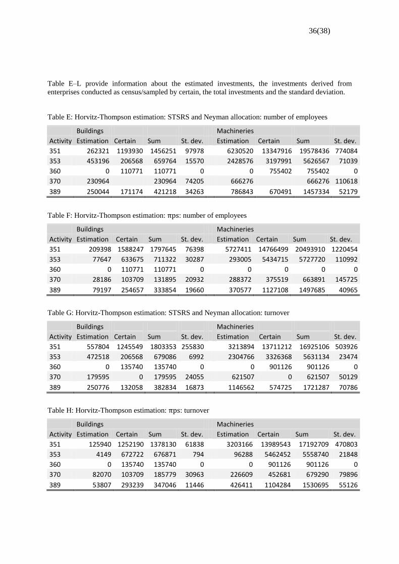
36(38)

*

Table E–L provide information about the estimated investments, the investments derived from

enterprises conducted as census/sampled by certain, the total investments and the standard deviation.

Table E: Horvitz-Thompson estimation: STSRS and Neyman allocation: number of employees

Buildings Machineries

Activity Estimation Certain Sum St. dev. Estimation Certain Sum St. dev.

351 262321 1193930 1456251 97978

6230520 13347916 19578436 774084

353 453196 206568 659764 15570 2428576 3197991 5626567 71039

360 0 110771 110771 0

0 755402 755402 0

370 230964 230964 74205 666276 666276 110618

389 250044 171174 421218 34263 786843 670491 1457334 52179

Table F: Horvitz-Thompson estimation: : number of employees

Buildings Machineries

Activity Estimation Certain Sum St. dev. Estimation Certain Sum St. dev.

351 209398 1588247 1797645 76398

5727411 14766499 20493910 1220454

353 77647 633675 711322 30287 293005 5434715 5727720 110992

360 0 110771 110771 0

0 0 0 0

370 28186 103709 131895 20932 288372 375519 663891 145725

389 79197 254657 333854 19660 370577 1127108 1497685 40965

Table G: Horvitz-Thompson estimation: STSRS and Neyman allocation: turnover

Buildings Machineries

Activity Estimation Certain Sum St. dev. Estimation Certain Sum St. dev.

351 557804 1245549 1803353 255830

3213894 13711212 16925106 503926

353 472518 206568 679086 6992 2304766 3326368 5631134 23474

360 0 135740 135740 0

0 901126 901126 0

370 179595 0 179595 24055 621507 0 621507 50129

389 250776 132058 382834 16873 1146562 574725 1721287 70786

Table H: Horvitz-Thompson estimation: : turnover

Buildings Machineries

Activity Estimation Certain Sum St. dev. Estimation Certain Sum St. dev.

351 125940 1252190 1378130 61838

3203166 13989543 17192709 470803

353 4149 672722 676871 794 96288 5462452 5558740 21848

360 0 135740 135740 0

0 901126 901126 0

370 82070 103709 185779 30963 226609 452681 679290 79896

389 53807 293239 347046 11446 426411 1104284 1530695 55126

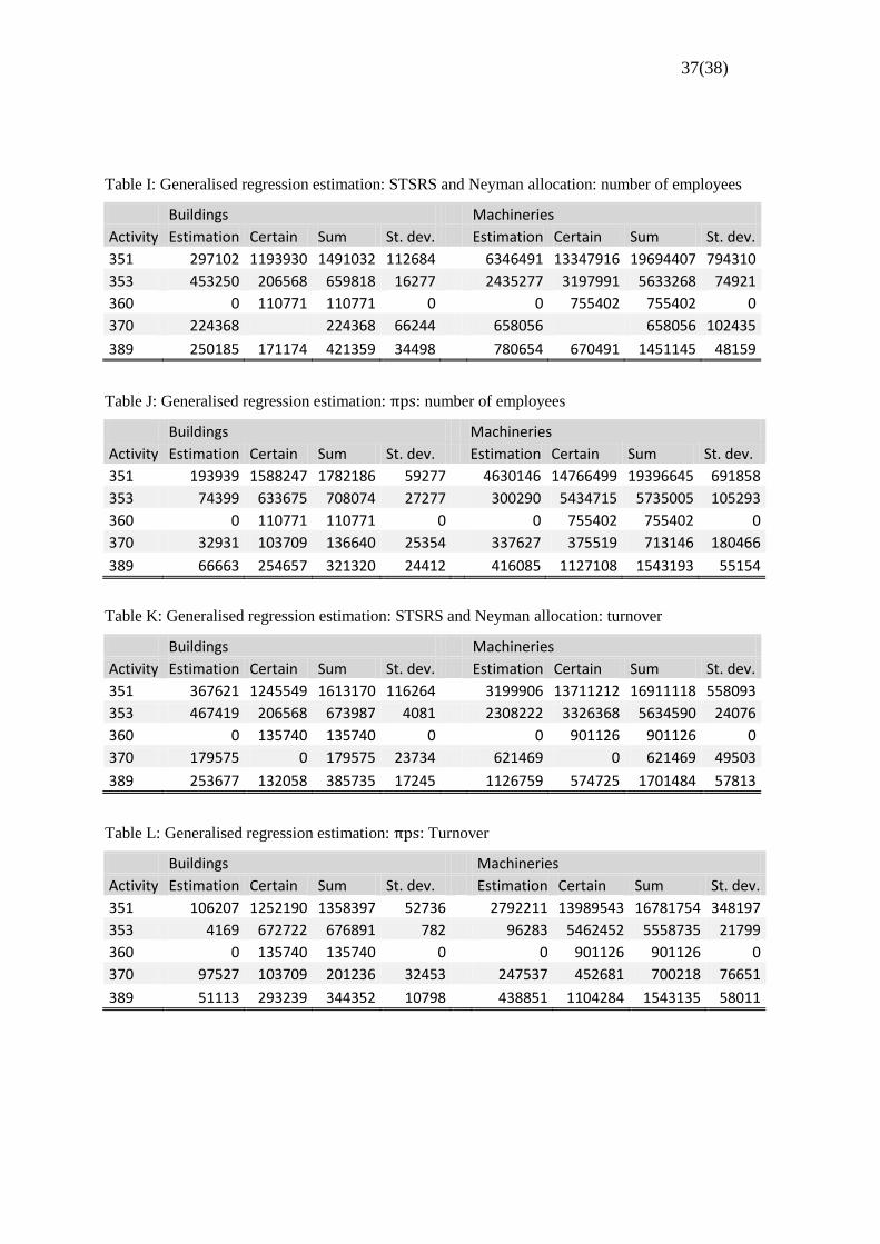
37(38)

*

Table I: Generalised regression estimation: STSRS and Neyman allocation: number of employees

Buildings Machineries

Activity Estimation Certain Sum St. dev. Estimation Certain Sum St. dev.

351 297102 1193930 1491032 112684

6346491 13347916 19694407 794310

353 453250 206568 659818 16277 2435277 3197991 5633268 74921

360 0 110771 110771 0

0 755402 755402 0

370 224368 224368 66244 658056 658056 102435

389 250185 171174 421359 34498 780654 670491 1451145 48159

Table J: Generalised regression estimation: : number of employees

Buildings Machineries

Activity Estimation Certain Sum St. dev. Estimation Certain Sum St. dev.

351 193939 1588247 1782186 59277

4630146 14766499 19396645 691858

353 74399 633675 708074 27277 300290 5434715 5735005 105293

360 0 110771 110771 0

0 755402 755402 0

370 32931 103709 136640 25354 337627 375519 713146 180466

389 66663 254657 321320 24412 416085 1127108 1543193 55154

Table K: Generalised regression estimation: STSRS and Neyman allocation: turnover

Buildings Machineries

Activity Estimation Certain Sum St. dev. Estimation Certain Sum St. dev.

351 367621 1245549 1613170 116264

3199906 13711212 16911118 558093

353 467419 206568 673987 4081 2308222 3326368 5634590 24076

360 0 135740 135740 0

0 901126 901126 0

370 179575 0 179575 23734 621469 0 621469 49503

389 253677 132058 385735 17245 1126759 574725 1701484 57813

Table L: Generalised regression estimation: : Turnover

Buildings Machineries

Activity Estimation Certain Sum St. dev. Estimation Certain Sum St. dev.

351 106207 1252190 1358397 52736

2792211 13989543 16781754 348197

353 4169 672722 676891 782 96283 5462452 5558735 21799

360 0 135740 135740 0

0 901126 901126 0

370 97527 103709 201236 32453 247537 452681 700218 76651

389 51113 293239 344352 10798 438851 1104284 1543135 58011

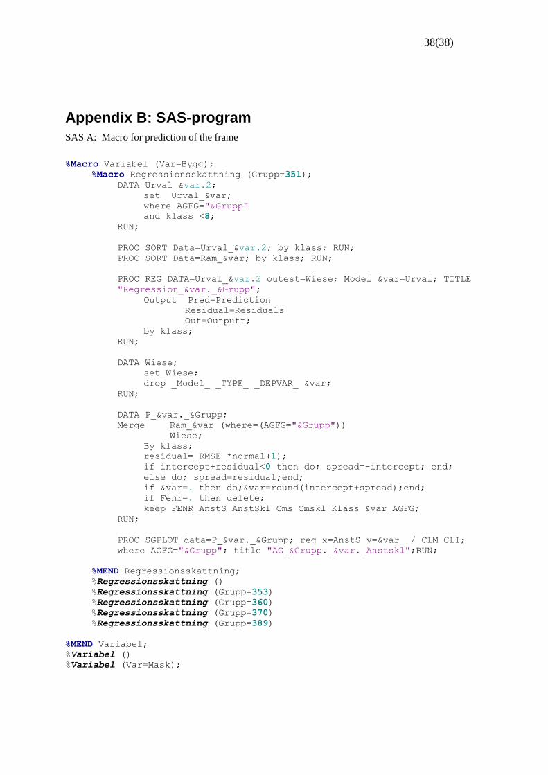
38(38)

*

Appendix B: SAS-program

SAS A: Macro for prediction of the frame

%Macro Variabel (Var=Bygg);

%Macro Regressionsskattning (Grupp=351);

DATA Urval_&var.2;

set Urval_&var;

where AGFG="&Grupp"

and klass <8;

RUN;

PROC SORT Data=Urval_&var.2; by klass; RUN;

PROC SORT Data=Ram_&var; by klass; RUN;

PROC REG DATA=Urval_&var.2 outest=Wiese; Model &var=Urval; TITLE

"Regression_&var._&Grupp";

Output Pred=Prediction

Residual=Residuals

Out=Outputt;

by klass;

RUN;

DATA Wiese;

set Wiese;

drop _Model_ _TYPE_ _DEPVAR_ &var;

RUN;

DATA P_&var._&Grupp;

Merge Ram_&var (where=(AGFG="&Grupp"))

Wiese;

By klass;

residual=_RMSE_*normal(1);

if intercept+residual<0 then do; spread=-intercept; end;

else do; spread=residual;end;

if &var=. then do;&var=round(intercept+spread);end;

if Fenr=. then delete;

keep FENR AnstS AnstSkl Oms Omskl Klass &var AGFG;

RUN;

PROC SGPLOT data=P_&var._&Grupp; reg x=AnstS y=&var / CLM CLI;

where AGFG="&Grupp"; title "AG_&Grupp._&var._Anstskl";RUN;

%MEND Regressionsskattning;

%Regressionsskattning ()

%Regressionsskattning (Grupp=353)

%Regressionsskattning (Grupp=360)

%Regressionsskattning (Grupp=370)

%Regressionsskattning (Grupp=389)

%MEND Variabel;

%Variabel ()

%Variabel (Var=Mask);