STRATHCLYDE

DISCUSSION PAPERS IN ECONOMICS

DEPARTMENT OF ECONOMICS UNIVERSITY OF STRATHCLYDE

GLASGOW

JOINT ESTIMATES OF AUTOMATIC AND DISCRETIONARY

FISCAL POLICY FOR THE OECD

BY

JULIA DARBY AND JACQUES MELITZ

NO. 11-22

Joint estimates of automatic and discretionary fiscal policy for the OECD

Julia Darby and Jacques Melitz*

This version – March 2011

Abstract

Official calculations of automatic stabilizers are seriously flawed since they rest on the

assumption that the only element of social spending that reacts automatically to the cycle is

unemployment compensation. This puts into question many estimates of discretionary fiscal

policy. In response, we propose a simultaneous estimate of automatic and discretionary fiscal

policy. This leads us, quite naturally, to a tripartite decomposition of the budget balance

between revenues, social spending and other spending as a bare minimum. Our headline

results for a panel of 20 OECD countries in 1981-2003 are .59 automatic stabilization in

percentage-points of primary surplus balances. All of this stabilization remains following

discretionary responses during contractions, but arguably only about 3/5 of it remains so in

expansions while discretionary behavior cancels the rest. We pay a lot of attention to the

impact of the Maastricht Treaty and the SGP on the EU members of our sample and to real

time data.

The authors would like to thank Kit Baum, Roel Beetsma, Jacopo Cimadomo, Rodolphe Desbordes, Andrew Hughes Hallett, Sandro Momigliano, Marcos Poplawski Ribeiro, participants at the 2011 EMF Conference in York and members of the Heriot-Watt economics seminar for valuable comments.

1

1. Introduction

Official figures for cyclically adjusted government budget balances rest on the assumption

that automatic fiscal policy essentially works through taxes and unemployment compensation.

The major international organizations, including the OECD, the IMF and the EU, and many

national governments within the OECD proceed on this assumption. In a review article,

Golinelli and Momigliano (2009) provide a long list of econometric studies that employ the

resulting official data for cyclically-adjusted budget balances. Yet there is little theoretical

and empirical support for this approach. Various other components of government spending

besides unemployment compensation may, in principle, respond automatically to the cycle.

Workers may retire earlier in recessions and later in expansions. The evidence for the OECD

indicates that they do. People facing job loss or temporary lay-off during a recession may be

eligible for invalidity benefits or sick pay as an alternative to unemployment benefits. There

has been a trend toward greater spending on invalidity benefits in many OECD countries in

recent decades. Therefore, invalidity benefits and sick pay might now move in sync with

unemployment compensation over the cycle. There is evidence that invalidity payments do.

Finally, according to the indications, personal health care varies counter-cyclically or, in other

words, inversely with the opportunity cost of time, which is higher in expansions than

recessions. Consequently, social spending on health care moves in a stabilizing manner over

the cycle.1 In Darby and Melitz (2008), we discussed this reasoning and the evidence at some

length and we shall confirm our earlier findings below. As a result, official figures for

cyclically adjusted government deficits should not serve in studying discretionary fiscal

policy. Unreliable inferences about discretionary policy will follow since the officially

adjusted figures fail to remove all the automatic responses of the fiscal aggregates.

Admittedly, not all studies proceed in this way, even when they do not question the usual

view. Many studies of discretionary fiscal policy apply various filters to construct their own

cyclically-adjusted budget balances. See, for example, Alesina et al. (2002), Lane (2003),

Aghion and Marinescu (2007), Beetsma and Giuliodori (2010) and Alesina and Ardagna 1 This spending refers to payments for insured health services provided to individuals or spending on entitlements, not to the wage bill or capital expenditures in a nationalized health sector. The latter are not included in the social spending data.

2

(2010). In these cases, the cyclically adjusted balances will reflect all responses of

government social spending to the cycle and our previous complaint does not hold. The only

objection we still retain concerns the attempt to construct cyclically adjusted data as a

preliminary prior to the study of discretionary fiscal policy responses. This two-step

procedure makes some untested assumptions about independence in the data. Joint estimation

of automatic and discretionary fiscal policy action over the cycle is better. This then defines

the primary objective of our study: to study both automatic and discretionary fiscal policy

jointly. However, this objective leads to another. If automatic and discretionary fiscal policy

are to be estimated jointly, it becomes difficult to justify dealing with the government surplus

as a single aggregate, rather than separating out some of its parts. The automatic responses of

fiscal policy to the cycle differ too widely on the revenue and expenditure sides. Social

spending might also need to be treated separately rather than lumped together with the rest of

government spending, or alternatively deducted from revenues after trimming social spending

down to transfer payments in order to construct net taxes. So the minimum decomposition of

the government budget therefore becomes a central issue as well. We shall attempt to study

automatic and discretionary fiscal policy jointly with the minimal decomposition of the

government budget for a sample of 20 OECD countries over the period 1981-2003.

We are not the first to propose estimating automatic and discretionary fiscal policy jointly:

Celasun et al. (2007) and Bernoth et al. (2008) do so too.2 Both of them simply use a different

identification rule than ours for distinguishing between automatic and discretionary fiscal

policy. Celasun et al. suppose that all common effects on primary surpluses across countries

are automatic while the idiosyncratic national ones are discretionary. Bernoth et al. separate

2There are also many studies of fiscal policy that simply make no distinction between automatic and discretionary responses and use unadjusted budget data as the dependent variable (though they may sometimes draw inferences about one sort of response or the other based on the results, for example, the source of influence on the budget). See for example Arreaza et al (1999) and Balassone and Francese (2004) or Balassone et al. (2008). Celasun et al. (2007) and Bernoth et al. (2008) are simply the only previous studies, to our knowledge, that explicitly try to estimate automatic and discretionary fiscal policy simultaneously from the start. In addition, Romer and Romer have recently proposed a new approach to discretionary fiscal policy responses to the cycle, their so-called “narrative” approach that, in principle, permits studying this one aspect of discretionary fiscal policy independently of automatic fiscal policy. Thus far, they have applied their approach only to tax policy in the US (Romer and Romer (2009, 2010)). But the IMF has already extended their approach to government spending and a wide international sample of countries (IMF (2010)).

3

automatic and discretionary responses to the cycle based on the differences between real time

and final data. More precisely they use the differences between real time and final data about

the output gap to identify discretionary responses while employing the final data to capture

the automatic responses. We base our identification strategy on the timing of responses to the

business cycle. By and large, automatic fiscal policy occurs more quickly than discretionary

fiscal policy. Accordingly, our basic procedure is to try to capture the difference between the

current calendar year response of different budgetary items to the cycle and the lagged one-

year response. No simple decomposition of the automatic and the discretionary responses

follows, since some current fiscal responses may be discretionary and some lagged responses

may be automatic. Indeed, there are grounds to think that some effects of the business cycle

on revenues and unemployment compensation occur only after the current year based on

existing legal rules, and this is perhaps especially true for unemployment compensation if, as

in our case, the relevant definition of the cycle is the OECD one, which rests on the output

gap rather than the Blanchard (1990) one, which rests on unemployment. However, only the

results can tell how serious the ambiguities are. We shall reason, based on the results, that

there are few ambiguities. A fairly clear distinction between automatic and discretionary

fiscal policy responses will emerge.

There is now also an important movement afoot to use real time data to identify discretionary

fiscal policy responses to the cycle, to which Bernoth et al. belong. Except for them and

Kalckreuth and Wolff (2007), the other authors in this movement begin with the official

figures for cyclically adjusted budget balances. See Forni and Momigiliano (2005), Golinelli

and Momigliano (2006, 2009), Cimadomo (2007), Giuliodori and Beetsma (2008), and

Beetsma and Giuliodori (2008). Yet it is not clear to us that the real time data is necessarily

superior to the final data. Observers and officials differ in their perceptions of current output

gaps, and decision-makers know that current output gap data are subject to large revisions.

Therefore, discretionary fiscal policy may rest on a broader assessment of the evidence than

the real time figures published by the OECD for the current output gap provide. As a result,

the lagged values of the final data that eventually emerge could provide as good or better

4

grounds for analyzing official intentions than the real time data does. This is an open issue, in

our eyes. A further consideration is that real time data are not available for our entire study

period but only for a sub-section, since 1993, so its exclusive use would have limited our

study greatly. We will use the available post-1993 sub-sample to check on our conclusions

about automatic and discretionary fiscal policy in our full sample.

Contrary to many studies of fiscal policy, though not all (see Golinelli and Momigliano

(2009)), we estimate our fiscal reaction function in first differences. One reason is the evident

non-stationarity of the data in levels. Another is our primary concern with the temporary

fiscal responses to the cycle. Many structural factors will affect the budget balance in levels,

but these structural influences should matter less in first differences, while the cyclical

influences should remain as important. We also avoid the introduction of the lagged

dependent variable, which figures in many other works. Apart from the well-known

objections to this variable in panel estimation based on statistical bias, the variable would

greatly complicate our distinction between the automatic and discretionary policy responses.

Several earlier studies of fiscal policy behavior employed a dynamic panel estimator,

Blundell-Bond. However, ours is an unbalanced panel of only 23 annual observations at most

for 20 countries; so such estimators are not attractive.3 For panels such as ours, we believe a

simpler version of GMM is superior, namely, an IV-GMM procedure providing standard

errors that are robust to serial correlation and that make no assumptions about

heteroskedasticity (see Baum et al. (2003) on this point). In the end, we also find that simple

IV estimates with correction for heteroskedasticity yield results that are virtually

3 These studies may have been motivated by a desire to avoid large sample bias in panel estimation resulting from the correlation of the lagged dependent variable with the error term (see Nickell (1981)) since the studies tend to introduce the lagged dependent variable. It is however important to remember that dynamic panel data (DPD) techniques, including Blundell-Bond’s system GMM estimator, were designed for panels with many cross-sectional units N, whether countries, firms or people. The consistency of the DPD estimators was first established under the assumption of a fixed time dimension T but N tending to infinity. More recently, however, Bun and Kiviet (2006) examined the performance of a number of dynamic panel techniques in samples where both T and N are only moderate or small, as is true in our tests, and reported that in these circumstances "all dynamic panel techniques show substantial bias… so standard first-order asymptotic theory is of little use in ranking the qualities”. Furthermore Cameron and Trivedi (2005) warn that the application of Blundell Bond style estimators to panels with small N can, in practice, lead to a large loss of efficiency while masking problems associated with weak instruments. This last warning concerns us since we instrument.

5

indistinguishable from IV-GMM estimates.4 Since there is therefore only negligible gain in

efficiency from IV-GMM, simple panel IV results are the ones that we report below.

Following Galí and Perotti (2002), virtually all studies of fiscal policy behavior tend to

instrument the output gap in order to avoid simultaneity bias. We do the same.

As a final introductory note, we may return to the issue of the proper degree of aggregation. It

is generally recognized that taxes move up with output regardless of cyclical upswings or

secular growth whereas government consumption and investment may not go up with cyclical

upswings but only with economic growth. Moreover, some parts of social spending can be

expected to go down during a boom while going up with secular growth. This is true of

unemployment compensation, and based on our opening paragraph, might be true as well of

other parts of social spending. On these grounds, any single-aggregate approach to

discretionary and automatic fiscal policy cannot be simply taken for granted and could well

be overly restrictive and possibly misleading.

The next section will lay out our fundamental econometric model. Following, we shall offer

separate estimates of automatic stabilization for unemployment compensation and other

elements of social expenditure. These estimates will proceed from our fundamental approach,

but they have no purpose other than to underline our opening message of the need to extend

the analysis of automatic stabilization beyond unemployment compensation to many other

parts of social spending. Our preferred estimates of automatic stabilization follow in the next

section, IV, where we consider automatic and discretionary fiscal policy jointly. In that

section we also treat social expenditures as a separate aggregate. Section V introduces

asymmetric responses to expansions and recessions over the cycle. The results of this section

notably qualify those in the preceding section IV. Section VI next considers the effects of the

Maastricht Treaty and the Stability and Growth Pact in the EMU. Section VII discusses the

impact of real time data. Section VIII concludes.

A summary of the results

4 We carried out both sets of IV estimates with Stata 11, using ivreg2 routines to generate the IV-GMM ones; see Baum et al. (2010), and Roodman (2003, 2009).

6

Our baseline estimate of automatic stabilization is .59. Specifically, a one percent increase in

output relative to potential output raises the net primary surplus by .59 of one percent of

output. Given our choice of specification in terms of ratios of output, the results imply that

any contribution of government receipts must hinge on changes in the progressivity of

taxation over the cycle, for which we find inadequate evidence. Thus, the estimated

stabilization shows up essentially on the spending side (compare Arreaza et al. (1999)).

According to our estimate, a one per cent rise in output relative to potential output raises

government spending on goods and services exclusive of health by .24 of a percentage-point

of output and raises social expenditures by .35 of a percentage-point of output. However, in

the following year, discretionary policy offsets the entire automatic response stemming from

government consumption in an expansion, possibly entirely, whereas no similar offset takes

place in a contraction. As a result, the .59 automatic stabilization remains standing following

discretionary action in a contraction whereas as little as .35 may remain in an expansion. In

addition, though the total stabilization coming from both automatic and discretionary policy

combined is divided between social spending and other government spending roughly in a

ratio of 3:2 in a contraction, during an expansion still more of the stabilization and possibly

all of it comes from social spending (compare Hercowitz and Strawczynski (2004)). This

asymmetry in the response of fiscal policy must induce deficit spending over the cycle, in

accordance with the widespread thesis of a deficit bias over the cycle (see Roubini and Sachs

(1989), Grilli et al. (1991), Alesina and Perotti (1995) von Hagen and Harden (1995), de Haan

et al (1999) Kontopoulos and Perotti (1999), and Velasco (1999)). Our finding also supports

the frequent view that EU members tend to neutralize automatic stabilization through

discretionary fiscal policy during expansions (see Buti and Sapir (1998), Fatas and Mihov

(2003a, b), Balassone and Francese (2004), and Balassone et al (2008)). Note, however, that

we do not support the extreme conclusion, occasionally found, of a complete neutralization of

automatic stabilization during expansions.

To continue with the discussion of the results for stabilization policy, we find no “fiscal drag”

resulting from inflation over the cycle. This “drag” refers to the idea that current inflation

7

automatically leads to net government surpluses on a secular basis, as taxes move up in step

with inflation ̶ or even faster through “bracket creep” ̶ whereas spending does not.

According to our results, there is indeed a “fiscal drag” on the spending side as neither

government social payments nor government consumption keep up with inflation. But there is

a comparable “drag” on the revenue side as taxes do not keep up with inflation either. It all

comes out even in the wash.

Besides the destabilizing behavior of discretionary fiscal policy during expansions, two other

discretionary influences of fiscal policy appear. One is a stabilizing response of the net

primary surplus to government debt. A one-percentage-point rise in debt relative to output

raises the primary surplus (conservatively) by .022 of one percentage-point of output. This

accords with much recent work (see Melitz (1997), Bohn (1998), Ballabriga and Martinez-

Mongay (2002), Galí and Perotti (2003), Annett (2006), Mendoza and Ostry (2007),

Balassone et al. (2008), Candelon et al (2010)).

The second discretionary influence that we found is the impact of an election year. In line

with a great deal of earlier research, in an election year, tax revenues tend to fall (see Annett

(2006), Golinelli and Momigliano (2006), Candelon et al (2010)). If anything, the effects on

government consumption and social spending are positive but insignificant at conventional

levels. No other political influence emerges, despite the fact that many other such influences

appear in the rich literature on the political influences on government deficit spending (for

references, see Annett (2006), and, for example, Hallerberg and von Hagen (1999)). Perhaps

the failure of these variables to enter is related to our move to first differences which

eliminates all country-specific fixed effects on levels of government receipts and

expenditures.

For similar reasons, which may be magnified by our instrumentation of output gaps, we have

had no success finding any impact of the Maastricht Treaty and the SGP on the fiscal

behavior of EMU members, even in the 1993-1998 period, when efforts to qualify for entry

into EMU are widely believed to have reduced fiscal deficits.

8

Finally, our key results survive when we introduce real time data despite the consequent sharp

reduction in time-span. We cannot say anything about asymmetry in this case, since

regardless of final or real time data, the results are too weak for the shorter period. But

otherwise our estimates of automatic fiscal policy and our conclusions about discretionary

fiscal policy responses to the cycle are little affected.

II. The test specification

Preliminaries

Official estimates of automatic stabilization proceed in levels and provide the number of cents

of net government surplus resulting from a dollar of output gap (GDP minus potential GDP).

By contrast, estimates of discretionary fiscal policy responses to the cycle usually proceed in

ratios. They provide the fraction of a percentage point of net government surplus relative to

(divided by) output or potential output resulting from a percentage point of output gap relative

to (divided by) output or potential output. All the studies we cited earlier that construct their

own cyclically-adjusted data for the net primary surplus proceed in ratios. In the numerous

instances where the choice is simply to import the official series for cyclically adjusted

budget balances (which are in levels), the tendency is to divide by output or potential output

as a separate step prior to turning to the analysis of discretionary fiscal policy (for example,

Galí and Perotti (2003)). Since we estimate automatic and discretionary policy

simultaneously, we must make a choice. Ours is to use the percentage formulation. While this

changes nothing fundamental, it does dwarf the contribution of receipts to automatic

stabilization relative to the contribution of spending. Simple as it is, this point deserves major

attention.

Take the simple classroom example of proportional taxation and total independence of

spending from the cycle. If we proceed in levels, taxes respond to the output gap in a

stabilizing manner and government spending does not. Taxes rise while government spending

stands still in an expansion. If we proceed in ratios, spending responds to the output gap in a

stabilizing manner whereas taxes do not. The ratio of government spending to output falls

while the ratio of government receipts stands still in an expansion. The fundamental truth is

9

that the stabilization depends entirely on the combination of proportional taxation and cyclical

inertia of spending in both examples. Without both together − and in particular if spending

automatically followed output over the cycle like taxes − then there would be no automatic

stabilization regardless of estimate in levels or ratios in the case of a balanced budget and

with minor qualification otherwise.

We will therefore attach little significance, if any, to our results about the lack of contribution

of taxes to automatic stabilization relative to government expenditures. On the other hand, our

results for the behavior of different sources of government revenue relative to one another

will deserve emphasis. So will our results about the relative contributions of different

components of spending relative to one another. This last point, concerning spending,

deserves particular emphasis. We see reason to expect some automatic counter-cyclical

movement of social spending in level form and we see no reason to expect any automatic

counter-cyclical movement of government consumption in level form. Therefore, we expect a

higher contribution of social spending to automatic stabilization than government

consumption in level form. But if so, we must also expect the same in ratios or after we divide

both spending and output gaps by output.

The test specification

With these points in mind, our basic estimating equations for the fiscal policy reaction

functions can be expressed as follows:

tjitjitj

tjitji

tj

tji

tj

tjiiti

tj

tji elecYD

Y

Y

Y

YYX

εββπβββαα ++⎟⎟⎠

⎞⎜⎜⎝

⎛+Δ+

⎟⎟

⎠

⎞

⎜⎜

⎝

⎛Δ+

⎟⎟

⎠

⎞

⎜⎜

⎝

⎛Δ++=⎟

⎟⎠

⎞⎜⎜⎝

⎛Δ

−

−

−

−5

1

143*

1

12*1 (1)

X refers either to the primary budget surplus or the disaggregated components of the primary

budget surplus. In case of disaggregation, there are as many equations (1) as components i.

Subscript j refers to the country and t to time. αt refers to time fixed effects. Y refers to GDP,

Y* to potential GDP, π to inflation (calculated using the GDP deflator), D to total public debt,

and elec is a dummy variable equal 1 in the year of a national election in country j and zero

10

otherwise. As indicated previously, we expect βi1 to be positive for the primary surplus and

for government spending, if only because of automatic effects, but we are agnostic about it for

revenues and we are agnostic about βi2 in general. The reason for using the primary budget

surplus rather than the observed budget surplus as the dependent variable (either as a single

aggregate or as the sum of the relevant parts) is our interest in βi4, that is, the response of the

budget to the previous year’s debt to GDP ratio. Given this dependent variable, Bohn (1998,

2005) has shown that if the equation for the primary surplus is properly specified or contains

all the proper explanatory variables on the right hand side, a positive value of β4, however

low, is a sufficient condition (not a necessary one) for the solvency of the government. We

experimented with a number of other political and economic variables besides elec that move

over time, including openness, but the dummy variable for the years of a national election,

elec, is the only one that we retain. As we noted earlier, many studies have provided strong

political reasons to expect βi5 to be negative (in its effect on the primary surplus). Earlier

empirical work would also lead one to expect negative values for this coefficient as well as

positive ones for βi4 (in their respective effects on the primary surplus) for OECD countries.

We have already explained our decision to exclude the lagged dependent variable from the

regressions, both for econometric reasons and because of our intended interpretation of βi1

and βi2.5 In addition, as a result of our decision to proceed in first differences, there is no

need for country-specific influences. Such influences would merely use up degrees of

freedom but otherwise have no effect, at least in principle (see Cameron and Trivedi (2005,

pp. 781ff.) and Roodman (2009)).6

We initially instrumented all the first four variables in equations (1) in the estimates.

However, test statistics consistently failed to reject the weak exogeneity of the inflation

variable. Thus, in the end, we only retained instruments for the two output gap variables and

the debt/GDP ratio. These instruments are 2, 3 and 4-period lags of (Y/Y*)t and 2 and 3- 5 We did experiment with the second lag in the dependent variable, since at this lag length there would be no clear interference with our intended interpretation of βi1 and βi2 and the variable could reflect omitted influences in the rest of the equation. At this lag length, the lagged dependent variable is insignificant, whether we instrument it or not. 6 We added country-specific effects in Darby and Melitz (2008) but they indeed made no difference.

11

period lags of (D/Y)t-1. This economy of instruments proved valuable in estimation. Our basic

data sources are the OECD, the Economic Outlook and Social Expenditure databases, except

for elec which comes from Armingeon et al. (2008).

The twenty countries in the sample are Australia, Austria, Belgium, Canada, Denmark,

Finland, France, Germany, Iceland, Ireland, Italy, Japan, the Netherlands, New Zealand,

Norway, Portugal, Spain, Sweden, the UK and the US. Ours is an unbalanced panel for 1981-

2003 at best. We could have extended the study prior to 1981 and beyond 2003 had we not

been keen on using a series for social spending inclusive of health expenditure.7 Our measures

of Y* and the output gap Y/Y* rely upon the OECD’s measure of potential output. But we

have experimented with HP filtered data and the use of cubic spline functions to represent the

long run secular trend in output or potential output instead.

III. The automatic responses of social spending

We begin discussion of the results with a simple confirmation of our starting message that

automatic stabilization issues from many parts of social spending and not only unemployment

compensation. Consider equations (1) for the spending items Xi consisting of unemployment

compensation, pensions, health spending, incapacity benefits and sick pay after dropping all

explanatory variables reflecting strictly discretionary action, and also dropping the lagged

output gap. Dropping the lagged output gap could well remove some automatic stabilization.

Yet even if it does, the resulting estimates should still reflect automatic responses alone, since

the responses of social spending to the current output gap clearly depend on the application of

standing legal rules and we know of little evidence of short-term adjustment of these rules to

the cycle. The resulting equations are:

tjitjitj

tjiiti

tj

tji

Y

YY

Xεπββαα +Δ+

⎟⎟

⎠

⎞

⎜⎜

⎝

⎛Δ++=⎟

⎟⎠

⎞⎜⎜⎝

⎛Δ 2*1 (2)

Table 1 shows the separate IV estimates of equations (2) for the spending items in question.

7 Specifically, the series we use for government spending on health benefits comes from the OECD Social Expenditure database. This database is less frequently published than the Economic Outlook one and we accessed the 2007 release that only provides data going up to 2003.

12

The table only shows the estimates of βi1 or the automatic responses to the cycle. Standard

errors are robust to heteroskedasticity and autocorrelation, and Δ(Y/Y*) is instrumented in the

manner previously described and repeated at the bottom of the table.

Of course, these are not our preferred estimates of automatic stabilization, which only follow

from equations (1) where discretionary fiscal policy enters simultaneously. However, the

estimates of equations (2) are relevant in discussing the popular view that unemployment

compensation is the only major category of social spending that responds automatically to the

cycle since this view generally rests on estimates of automatic stabilization that exclude any

discretionary policy. We must also emphasize that the conclusions in table 1 do not depend on

our detailed estimation procedure. They would also follow if we used alternative measures of

potential output depending on HP-filtered data or after approximating long term trend output

via a spline function. They would similarly follow just as well if we introduced the lagged

dependent variable or if we used 3SLS. Our previous work (Darby and Melitz (2008)) already

cast much light on this point.

As seen from table 1, based on equations (2), the contribution of social spending to automatic

stabilization is .34 of a percentage-point relative to output. Consider instead the contribution

of unemployment compensation by itself. We get a value of only .08. This last contribution

thus makes up only about a quarter of the response of total social spending in the current

period. Separate estimates for the other elements of social spending follow. They show a

contribution of .12 of a percentage-point for pensions and one of around .06 of a percentage-

point for health spending. Given the confidence intervals, both figures are of a similar order

of magnitude to the one for unemployment compensation. The contribution of incapacity

benefits is also clear, though much smaller than any of the preceding. Sick pay is the one

category of social spending in Table 1 whose contribution to automatic stabilization does not

emerge. The sum of the individual contributions in the table does not add up to the total for

social spending partly because our disaggregated estimates omit subsidies to firms and other

miscellanea.

13

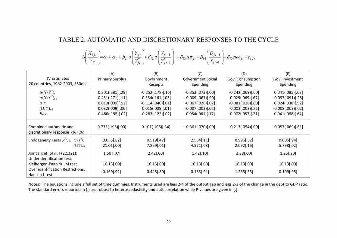
IV. Automatic and discretionary fiscal policy combined

We turn next to the central issue in this study of the joint estimation of automatic and

discretionary fiscal policy. Let us begin with the case of symmetric responses to cyclical

expansions and contractions, meaning equations (1). The relevant estimates are summarized

in Table 2. There will be some important modifications once we allow for asymmetry, but

these will strictly concern government consumption spending net of health. Table 2 offers

estimates of five selected equations. The first one (Part A) relates to the net primary surplus

and the next four pertain to our basic decomposition, which is between government receipts

(Part B), social expenditures including health (Part C), government consumption exclusive of

social health spending (Part D), and government investment (Part E). The equation for

investment is extremely unstable. None of its coefficients are significantly different from zero

apart from the −.01 for the debt ratio; and we shall center the discussion on the other four

equations. We shall also refer henceforth to government consumption exclusive of social

health spending simply as government consumption.

Let us focus first on the general test statistics. The performance of the instruments is

satisfactory in all four equations. There is no problem of under-identification. Furthermore,

the Hansen test of the joint null hypothesis that the instruments are uncorrelated with the error

term and that the excluded instruments are correctly excluded from the estimated equation, is

highly satisfactory. Interestingly enough, the tests of endogeneity reveal less need for

instruments than the use we make of them. The tests unambiguously fail to require rejecting

the null hypothesis of weak exogeneity of the contemporaneous output gap in all of the

equations except social spending. In the case of the debt/GDP ratio too, these tests reject the

null hypothesis of weak exogeneity in all the equations (with any ambiguity at all only in the

consumption one).

As regards the individual coefficients, let us consider first those reflecting the responses to the

business cycle, 1iβ and 2iβ . We shall also look carefully at the sum of these two coefficients,

21 ii ββ + , which concerns the total fiscal policy response to the cycle without any regard for

the time profile or the distinction between automatic and discretionary action. This sum and

14

its standard error both appear in the table right below all the individual coefficients. In the

case of the first four equations (Parts A through D), 21 ii ββ + is highly significant except for

revenues. In the case of the primary surplus, Part A, this sum is also extremely high, .73.

However, in Part A neither 1iβ nor 2iβ is individually significant at conventional levels. This

might be related to the result for revenue, in Part B, which shows opposite signs for the

current and lagged responses. There is a stabilizing lagged response 2iβ offsetting a (less well

defined) destabilizing current one 1iβ . If accepted, this see-saw movement could be

interpreted at least in two ways: a discretionary offset of an initial destabilizing automatic

effect or a lagged automatic offset of an initial destabilizing automatic effect. We lean toward

the latter interpretation. As mentioned earlier, some tax revenues can be expected to respond

to the cycle with a one year lag based on existing tax legislation. This could cause revenues

not to keep up with cyclical movements in output at first but to catch up a year later. On this

interpretation, the results for revenues correspond to proportional taxation following a year

(since 21 ii ββ + is insignificant). We have studied direct taxes on households, direct taxes on

firms, indirect taxes and social security revenues separately in order to see if this sheds any

more light on the issue but it does not. The same basic time profile and aggregate outcome

emerges for each separate category of revenues.

The results for government social spending and government consumption are the central ones.

In both cases, there is a well-defined response to the business cycle, which is entirely

concentrated in the current period. We see little reason to question in either case that the

response is entirely automatic. As mentioned before, in the case of social payments, the rules

of eligibility do not alter in a cyclical manner. As for government consumption, there is a

priori ground to expect an automatic counter-cyclical movement of the ratio to output and if

discretionary fiscal policy either amplified or attenuated this movement, we would have

expected the discretionary action not only to show up within the current year but also a year

later. On these grounds, we shall interpret the results of Parts C and D of table 2 to signify

strictly automatic stabilization, .35 coming from social spending and .24 more coming from

consumption spending.

15

There is no evidence of automatic effects of current inflation based on the estimates of the

primary surplus (Part A). This fits in well with the disaggregated results, showing significant

offsetting effects of inflation on the revenue and spending sides of roughly equal size. Ratios

of government revenues to output do not keep up with inflation but nor do ratios of taxes to

output.

With respect to debt, a stabilizing discretionary response of .022 shows up based on the 3-part

decomposition of receipts, social spending and consumption (which would be higher if we

admitted the single significant coefficient in the equation for investment), .015 of it coming

from taxes and less, only .007, from social spending. This is below the significant value of

.032 stabilization that we obtain in the single-equation estimate for the government primary

surplus (which may incorporate the figure for investment). In the light of Mendoza and Ostry

(2007) in particular, we also looked for non-linear effects of debt but found nothing.

As regards elections, the tendency of an election year to lead to looser fiscal policy emerges

plainly. A reduction in taxes is particularly clear. While any rise in government spending is

not, the estimate for elec in the net primary surplus equation closely resembles the one we get

by summing up the separate tax and spending coefficients and this value is also significant at

the 95 percent confidence level. We are therefore prone to accept the conclusion that a

national election raises the primary deficit relative to GDP by approximately one-half of one

percentage-point of output, that is, roughly the amount shown in the primary surplus equation.

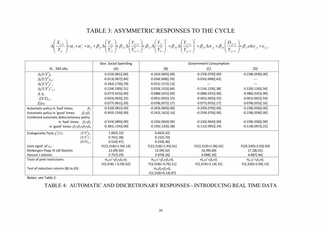
V. Asymmetric responses to the cycle

Political considerations offer strong reasons to suspect there might be asymmetric responses

to the business cycle, and more specifically, that fiscal discipline may relax substantially

during expansions. We can allow for such responses by controlling separately for ‘good

times’ (when Y>Y*) and ‘bad times’ when (Y<Y*). We shall do so by introducing three

additional variables in equation (1). The first is a dummy variable αi+ which is equal 1 when

Y>Y* and equal 0 otherwise. This allows for a separate intercept in ‘good times’ (αi + αi+) and

in ‘bad times’ (αi). We also add two interaction terms resulting by multiplying this dummy by

16

the output gap terms. Those generate Δ(Y/Y*)t+ and Δ(Y/Y*)t-1

+ values, which are simply the

values of Δ(Y/Y*)t and Δ(Y/Y*)t-1 when Y>Y* and equal 0 otherwise. The new test equation is

hence:

)3(71

165

*1

14*3*

1

12*1

tjitjitj

tjitji

tj

tji

tj

tji

tj

tji

tj

tjiitii

tj

tji

elecYD

Y

Y

Y

Y

Y

Y

Y

YYX

εββπβ

ββββααα

++⎟⎟⎠

⎞⎜⎜⎝

⎛+Δ+

⎟⎟

⎠

⎞

⎜⎜

⎝

⎛Δ+

⎟⎟

⎠

⎞

⎜⎜

⎝

⎛Δ+

⎟⎟

⎠

⎞

⎜⎜

⎝

⎛Δ+

⎟⎟

⎠

⎞

⎜⎜

⎝

⎛Δ+++=⎟

⎟⎠

⎞⎜⎜⎝

⎛Δ

−

−

+

−

−+

−

−+

An alternative approach to modeling asymmetric adjustment in some studies is to include

separate output gap terms for ‘good’ and ‘bad’ times instead a term applying at all times and

an additional term for in the output gap in ‘good’ times only, as we do. The implied responses

in ‘good’ and ‘bad’ times are identical in both cases, but our approach has the advantage that

the estimates of βi3 and βi4, and the associated tests of significance, show directly whether

there is a significant asymmetry while a separate test is necessary (for the significance of the

difference between the coefficients in ‘good’ and ‘bad’ times) in the alternative approach. We

also report an F-test of the joint restriction αi+= βi3 = βi4 = 0 to test the null hypothesis of

symmetry against the alternative of asymmetry.

In the estimates of equation (3), the results for the primary surplus are unacceptable based on

the Hansen J statistic, whose probability value falls close to zero. The overidentifying

conditions concerning the instruments can no longer be upheld. The results for government

revenues, for their part, are similar to the previous ones. Allowing for asymmetry in this

equation changes little. The results for social spending and consumption are the interesting

ones. We present them in the first two columns of table 3 (A and B).

In both columns (A) and (B) it is clear that the joint F-tests for αi+ = βi3 = βi4 = 0 fail to reject

the null hypothesis of symmetry. Notwithstanding, it is helpful to look more closely at the

implied responses in ‘good times’ and in ‘bad times’, since this is our primary concern. As

regards social spending, the automatic stabilization in ‘good times’ β1 + β3 appears to be just

as significant as in ‘bad times’ (for β1 alone). In addition, the combined automatic and

17

discretionary action in ‘good times’ β1 + β2 + β3 + β4 differs little from the combined

automatic and discretionary action in ‘bad times’ β1 + β2. Therefore the hypothesis of

symmetry seems sound. However, in the case of government consumption, things are

different. The high probability value of .38 associated with the combined automatic and

discretionary action in ‘good times’ would indicate insignificance, while the total effect in

‘bad times” is highly significant, with a probability value of .00. This clearly suggests an

important asymmetry. The next two columns of Table 3 investigate this possibility further.

Neither β2 nor β3 is significant in the case of government consumption in column B.

Accordingly suppose we set both coefficients equal to zero. In column C, we set β3 equal

zero, while in column D we additionally drop β2. Thus, column C simply imposes symmetry

in the current response to the cycle while column D additionally admits no lagged response to

the cycle in ‘bad times’. As can be seen, the estimates in these next 2 columns hardly differ at

all from column B. To be quite specific, the fiscal response in the current period, or the

automatic one, varies only between .23 and .26, regardless of ‘good’ or ‘bad times,’ in all 3

columns, and the estimates for the total effect in ‘good times’ are similarly uniform and

insignificant. Furthermore direct testing of the joint restrictions that are imposed by the

successive deletions of the two terms starting from the column B specification shows that the

restrictions cannot be rejected, as indicated by the F test. The key difference is that the

relevant hypothesis of zero asymmetry becomes less and less probable as we move from

column B to column C to column D. The probability-value for the F test of the corresponding

symmetry null F test goes down from .51 to .32 to .13 from B to C to D. Symmetry becomes

less plausible.

Based on the estimates of the simplified specification reported in column D (and the previous

two columns as well for that matter), there would seem to be a significant asymmetry in the

implied behavior of government consumption: we cannot even reject the hypothesis that

discretionary action totally offsets automatic stabilization. It also makes sense to attribute

such reversal to discretionary action. The alternative of supposing an automatic tendency for

government consumption to go into reverse and cancel its own earlier stabilizing movement

18

from one year to the next does not seem plausible. We are also not necessarily justified,

however, in going to the extreme conclusion that the discretionary offset of the automatic

response of government consumption is complete. Indeed, the standard confidence interval

indicates that a wide range of estimates of the combined automatic and discretionary effect

centered on the reported point estimate, cannot be rejected by the data. On this ground, the

most likely degree of reversal of the automatic effect is about half.

Based on the estimate for government consumption in column D of table 3, the earlier

estimates of the other influences on government consumption (table 2, column D), or those

for inflation, the debt ratio and the election years, are hardly affected.

If we combine the estimates for government revenues and social spending in table 2 in the

previous section with those for government consumption in table 3 in this section, we get the

basic results of our study that we reported in the introduction. There is .59 automatic

stabilization, .35 coming from social spending and the other .24 from government

consumption. The full .59 stabilization remains following the response of discretionary policy

in a contraction, but arguably, only .35 (out of 1) remains after this response in an expansion.

VI. The Maastricht Treaty and the Stability and Growth Pact

The Maastricht Treaty came into effect in 1993 and the Stability and Growth Pact (SGP) did

so late in 1997 or basically in 1998. Starting with Ballabriga and Martinez-Mongay (2002)

and Galí and Perotti (2003), a sizeable literature analyzes the possible effect of both on the

fiscal policy behavior of the EU members, the EMU members in particular. Galí and Perotti

found little difference for the EMU members to speak of. More recent results are mixed

(Balassone and Francese (2004), Forni and Momigliano (2005), Golinelli and Momigliano

(2006), Balassone et al (2008), Beetsma and Giuliodori (2008), Candelon et al (2010)). One

conclusion seems to stand out if any: namely, that the effort to meet the entry conditions of

the Maastricht Treaty led the candidate countries to rein in their budget deficits in 1993-1998,

whereas following entry, the Treaty and the SGP ceased to exert any disciplinary pressure

(see von Hagen et al (2000), IMF (2001), OECD (2005), Annett (2006), and Poplawski

19

Ribeiro (2009)). Even on this seeming point of agreement, there is no unanimity: Hercovitz

and Strawczynski (2005) rally to Galí and Perotti’s view (at least for government spending if

not the net primary surplus as a whole) in their statement: “We found that government

spending adjustment began in 1994, and that it can be characterized as an OECD phenomenon

rather than as a phenomenon specific to countries participating in the Maastricht Treaty or the

Stability and Growth Pact” (p.822).

In view of this literature, we made a strenuous effort to test for some differences in the

behavior of EMU members following Maastricht. We constructed a dummy variable for EMU

members that began with the Maastricht Treaty or candidacy for membership and covers

1993-2003 and interacted the variable with current and lagged changes in output gaps and, in

addition, we included the dummy separately. This mimics Galí and Perotti’s (2003)

procedure, except that they use variables for before and after Maastricht whereas we use

variables for the full-sample period and post-Maastricht (for the same reasons that we

mentioned in connection with asymmetry: namely, to facilitate the interpretation of the

statistical significance of the differences before and after Maastricht).8 In some cases, rather

than defining the Maastricht variables for the EMU members for the entire study period, we

defined them only for 1993-1998. This was meant to test whether Maastricht had an impact

during candidacy but ceased to have any thereafter. In addition, we borrowed the suggestion

of Forni and Momigliano (2005) (subsequently adopted by Beetsma and Giuliodori (2008)

and Poplawski Ribeiro (2009)) of including a variable for deficit to GDP ratios in excess of

the Maastricht limit of 3% in order to test whether trespassing the limit fostered fiscal

discipline in subsequent periods. We then included the relevant variable with a one-year lag

together with the previous Maastricht variables (alternatively, those for 1993-2003 and only

for 1993-1998) or by itself alone. None of these experiments was successful.

In no case could we find a difference in behavior before and after Maastricht, regardless

8Of course, there are other differences between our estimates and those of Galí and Perotti: they use the cyclically adjusted net primary balance (as a ratio of potential output) in levels as the dependent variable, employ a different dynamic structure and do not attempt to distinguish between current and lagged influences of the output gap.

20

whether we defined after-Maastricht as 1993-1999 only or the whole post-1993 period. In the

process, though, we did find a significant difference between the behavior of the (eventual)

EMU members and the rest for social spending, which we discuss in the appendix.

Our fundamental conclusion is that, whatever may be true about Maastricht and its effects, it

is not possible to find any influence of the Treaty following the introduction of first

differences and instruments for the output gap, at least thus far or until longer time series

become available.

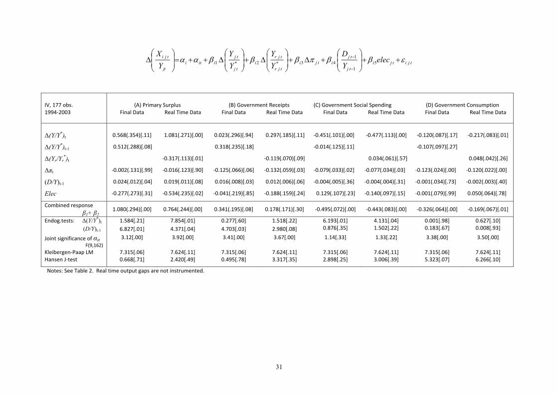
VII. The real time output gap

Finally, we turn to results incorporating real time data. The relevant data are taken from the

OECD’s forecast of output gaps that have been published annually in Economic Outlook since

1993. Our measure of the change in the real time output gap, Δ(Yr/Yr*)t, is the value of the

year t+1 forecast of Y/Y* published in the OECD’s December year t edition of Economic

Outloook, minus the year t forecast of Y/Y * published in the same edition. Since we use data

in first differences, the time period available for estimation is restricted to 1994 through to

2003, leaving 177 observations, approximately half as many as before. This drop in the span

of data is unfortunate, not least because it means that we are left trying to discriminate

between automatic and discretionary policy responses to the cycle in a period that

encompasses most of “the Great Moderation” or a period of low cyclical movement. We can

immediately infer that this will make the exercise more difficult. In order to draw any

inference, it is necessary first to reproduce the estimates in table 2, and those for government

consumption in table 3, for this reduced time span, for comparison. The effort to replicate the

earlier tests proves unsuccessful in the case of the asymmetric behavior of government

consumption in table 3. The conditions of under- and over-identification which relate to the

adequacy of the instruments are not sufficiently satisfied (the probability value of the

Kleibergen-Paap test statistic rises too much and that of the Hansen J statistics drops too low).

The revised estimates are uninformative. This should not be surprising. A loss of power is

bound to follow from the shorter sample, even apart from the cyclical calm in the part of the

sample that remains. Forging ahead with real time data does not help. We therefore center our

21

attention on table 2 concerning symmetry in all of the equations.

Estimates of the table 2 specification over the shorter 1994-2003 sample are set out in the

leftmost columns of each section of table 4 (in this case we ignore the investment equation,

which makes no difference for the subsequent comparisons). We shall alter the usual order of

discussion by beginning with social spending and consumption. As regards social spending,

the results correspond closely to the earlier ones in table 2. For government consumption,

matters are more complicated. The combined current and lagged response is similar in size to

the earlier one in the corresponding equation in table 2 and strongly significant, as it was

before. However, whilst in table 2 the entire impact was contemporaneous (automatic), in the

shorter sample the point estimates for the current and lagged effects are similar. Nonetheless

the considerable drop in the probability value for the Hansen J statistic conditions to .07 raises

doubt about the over-identifying restrictions and the validity of these estimates. On the other

hand and to complicate matters further, the case for instrumenting the output gaps becomes

particularly fragile based on the endogeneity test. Therefore, we experimented with

instrumenting only the debt ratio. In this case, none of the same difficulties arise. The results

for the decomposition between the current and lagged responses are similar to the previous

ones in table 2 and those for the aggregate of both responses continue to resemble the

common ones in tables 2 and 4. Switching to the new consumption equation therefore seems

unimportant. It also makes little difference for the subsequent comparison with the real time

results. In the end, we stick to the consumption equation in the table.

In the case of government revenues, shown in section (B) of table 4, it becomes possible to

accept a positive contribution to stabilization at the 90% confidence level for the shorter

sample. This may explain why the estimate of the total response of the primary surplus,

section (A), is now higher than before at 1.08. However, the impact of the cycle on the

primary surplus remains as difficult to decompose between a current and lagged response as it

was before. As for the other influences on government fiscal behavior, all in all, the only

notable difference is that the significance of the election year disappears.

22

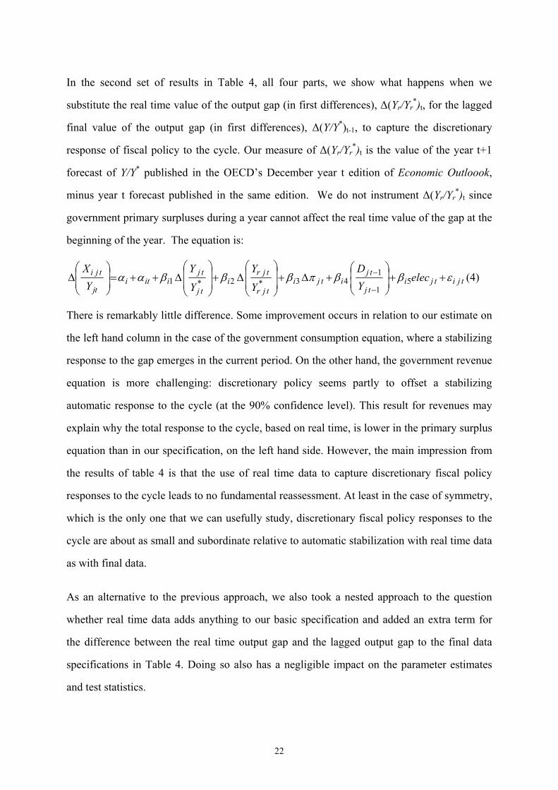
In the second set of results in Table 4, all four parts, we show what happens when we

substitute the real time value of the output gap (in first differences), Δ(Yr/Yr*)t, for the lagged

final value of the output gap (in first differences), Δ(Y/Y*)t-1, to capture the discretionary

response of fiscal policy to the cycle. Our measure of Δ(Yr/Yr*)t is the value of the year t+1

forecast of Y/Y* published in the OECD’s December year t edition of Economic Outloook,

minus year t forecast published in the same edition. We do not instrument Δ(Yr/Yr*)t since

government primary surpluses during a year cannot affect the real time value of the gap at the

beginning of the year. The equation is:

tjitjitj

tjitji

tjr

tjri

tj

tjiiti

tj

tji elecYD

Y

Y

Y

YY

Xεββπβββαα ++⎟

⎟⎠

⎞⎜⎜⎝

⎛+Δ+

⎟⎟

⎠

⎞

⎜⎜

⎝

⎛Δ+

⎟⎟

⎠

⎞

⎜⎜

⎝

⎛Δ++=⎟

⎟⎠

⎞⎜⎜⎝

⎛Δ

−

−5

1

143*2*1 (4)

There is remarkably little difference. Some improvement occurs in relation to our estimate on

the left hand column in the case of the government consumption equation, where a stabilizing

response to the gap emerges in the current period. On the other hand, the government revenue

equation is more challenging: discretionary policy seems partly to offset a stabilizing

automatic response to the cycle (at the 90% confidence level). This result for revenues may

explain why the total response to the cycle, based on real time, is lower in the primary surplus

equation than in our specification, on the left hand side. However, the main impression from

the results of table 4 is that the use of real time data to capture discretionary fiscal policy

responses to the cycle leads to no fundamental reassessment. At least in the case of symmetry,

which is the only one that we can usefully study, discretionary fiscal policy responses to the

cycle are about as small and subordinate relative to automatic stabilization with real time data

as with final data.

As an alternative to the previous approach, we also took a nested approach to the question

whether real time data adds anything to our basic specification and added an extra term for

the difference between the real time output gap and the lagged output gap to the final data

specifications in Table 4. Doing so also has a negligible impact on the parameter estimates

and test statistics.

23

However, our verdict does not agree with the earlier literature introducing real time data in

analyzing fiscal policy, where we encounter frequent suggestions that fiscal authorities try to

move in a stabilizing direction on the basis of real time data. In our view, though, the conflict

is smaller than it appears. It is plain only in the case of two studies: Kalckreuth and Wolff

(2007) and Bernoth et al. (2008).

In their lead-off article on fiscal policy based on real time data, Forni and Momigliano (2004)

only support the stabilizing movement of discretionary fiscal policy for contractions, not

expansions. Subsequent support of this stabilizing movement by Cimadomo (2007) and

Golinelli and Momigliano (2009) strictly concerns intentions rather than outcomes. Both

papers argue for stabilizing fiscal policy based on predicted values of primary government net

surpluses. Indeed, in the case of Cimadomo, the actual movement in the primary government

surpluses is even perverse: the surpluses move in the opposite direction to the intended. In the

case of Golinelli and Momigliano, things are not as bad: the authorities merely fail to obtain

the movement they desire in primary surpluses.9 Both papers effectively therefore contradict

Forni and Momigliano’s (2004) positive assessment of stabilizing discretionary policy

outcomes in contractions. Over and above this, all three studies and the rest concerning real

time responses of fiscal authorities to the cycle, with the exception of Kalckreuth and Wolff

(2007) and Bernoth et al. (2008), use official data for cyclically adjusted primary government

surpluses (whether final or in real time) as the dependent variable. Yet we have shown that

this data does not properly correct for the cycle. The studies also use real time data for the

output gap as the sole representation of the gap on the right hand sides. Yet the real time data

for the output gap, however distinct it may be from the final data, is still positively correlated

with it (anywhere from .40 to .62 in our sample). Thus, even so far as the results of these

studies intersect ours, the influence of the real time variable could well partly reflect

9 Both results are severely damning for discretionary fiscal policy responses to the cycle, especially those of Cimadomo, as he recognizes. It would be bad enough if the fiscal authorities did not succeed in moving the net primary surplus instrument in the intended direction. But if they even tend to move the surplus in the opposite way, they should clearly desist from any short run action. Indeed, even if the fiscal authorities control their instrument but merely significantly misinterpret the output gap in real time, questions already arise about discretionary fiscal policy in the short run. See, for example, Jonung and Larch (2006). We do not deal with any of these issues.

24

automatic rather than discretionary fiscal policy. Still another difference, of course, is that

these studies adopt a single-equation approach to fiscal behavior.

While the conflict between our results and the rest of the literature on real time is not clear in

the majority of cases, it is so for Kalckreuth and Wolff (2007) and Bernoth et al. (2008).

Kalckreuth and Wolff (2007) obtain discretionary responses of fiscal policy to real time errors

in the data about output (not the output gap) in the U.S.10 On their part, Bernoth et al. (2008)

report support for the stabilizing movement of fiscal policy in response to real time errors

about the output gap in a sample covering 14 European countries and most of our time span in

Table 4. For the moment, our only explanation for these differences is that Kalckreuth and

Wolff deal strictly with the U.S. and rely heavily on a different estimation method (SVAR)

whereas Bernoth et al. not only employ a different estimation method (Blundell-Bond GMM),

but a different specification (and their country/year sample also does not coincide with ours).

VIII. Conclusion

We have argued that official calculations of automatic stabilizers are seriously flawed. This

puts doubt on many estimates of discretionary fiscal policy responses to the cycle. One

approach is to avoid the official estimates but still retain the conventional two-step approach

to discretionary fiscal policy that consists of constructing cyclically adjusted data on the basis

of various filters for the cyclical adjustment in a first step. However, we believe that a better

solution is to estimate automatic and discretionary fiscal policy jointly from the start. One

consequence of our approach is to put into question any single-equation treatment of fiscal

policy since the revenues and spending sides respond widely differently to the cycle and since

the automatic responses of spending to the cycle depend heavily on most social spending.

This leads to a minimal three-part decomposition of the budget balance between revenues,

social spending, and spending on goods and services. However, we prefer a four-part

decomposition since the behavior of capital spending is sufficiently different. There is also an

argument for combining social spending on health with other social spending rather than

10 They also decompose government budget balances in two parts, net taxes (revenues minus transfer payments) and government spending on goods and services, as did Blanchard and Perotti (2002), in the study that serves them as a guide.

25

government consumption, where is it is usually found. Social spending on health responds

automatically to the cycle much like other social spending, consisting of transfer payments,

and not like government consumption. It is also a large and increasingly significant spending

item (around 13 percent of total government spending in the recent part of our OECD

sample). Unfortunately, though, OECD data series for social health spending (which strictly

relates to spending in response to claims by insured individuals and not any wage or capital

expenditures in a nationalized health sector, as explained in note 1) is only available from

1980 forward and published with far greater delays than the rest of the series in our study.

Therefore our insistence on reclassifying social health spending cuts down our estimation

period both at the beginning and the end.

Our headline results are .59 automatic stabilization in percentage-points of primary surplus

balances.11 In addition, discretionary policy cancels part of automatic stabilization through

destabilizing government consumption behavior (net of health) in expansions, leaving only

perhaps as little as .35 stabilization standing. On the other hand, the full influence of

automatic stabilization remains standing with no subsequent discretionary policy action in

contractions. These asymmetric results concerning government consumption fit in well with

many earlier theoretical and empirical findings. We also corroborate many earlier reports of

stabilizing responses of government budget balances to government debt and destabilizing

responses to national election dates, especially on the tax side. On the other hand, we fail to

confirm the occasional successes of earlier researchers in uncovering effects of the Maastricht

Treaty and the SGP on fiscal policy behavior in the eurozone and uncovering major

differences in responses of discretionary fiscal policy based on real time series. The reason

could lie in the greater demands that we make on the data via the use of first differences. The

shortness of our time series could also be a factor. Perhaps our use of instruments for the

separate influences of the output gap has something to do with the differences as well,

especially in light of the two previous factors. For these reasons, we only claim to be unable

11 The profiles of the cyclically adjusted budget balances for the individual countries based on our estimates are available upon request. They show far fewer long cyclical swings and many more reversals than the official series of the OECD though the two series are still positively correlated. We are grateful to David Cobham for suggesting that we examine this issue.

26

to confirm earlier conclusions about Maastricht influences or real time, not to refute them.

Let us note, in closing, that the recent upsurge of interest in fiscal policy following the 2007-

2009 financial crisis has increased the significance of a proper assessment of fiscal policy, a

large subject, to which we contribute. Without such assessment, efforts to detect the impact of

discretionary fiscal policy action on the economy cannot go far.

27

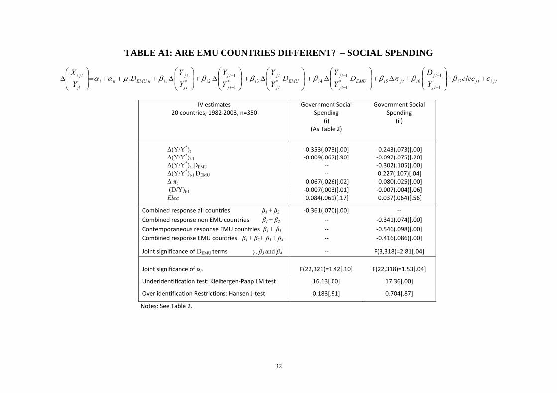
APPENDIX

Are EMU countries different? – Social and health spending

In the effort to uncover some difference in the behavior of (eventual) EMU members before

and after Maastricht, we introduced general controls for a difference in the behavior of the

EMU members from the rest for the period as a whole. While these controls made no

difference otherwise, they revealed a significant difference in behavior in the EMU for social

spending. The current response of social spending to the output gap in the EMU countries is

substantially more stabilizing than in the rest of the OECD, while the lagged response to the

gap in the EMU is somewhat destabilizing whereas outside the EMU it is not. In fact, there is

no significant lagged response to the gap at all outside EMU. Because of the destabilizing

lagged response in EMU, the combined current and lagged responses are only moderately

more stabilizing there than elsewhere. The result is in table A1 (column ii), where the

estimating equation is at the top.

As can be seen, for the current period, we get .55 stabilization for the EMU members (β1+β3)

and .24 (β1) for the rest. Once the lagged effects come into view, the sum stabilizing response

for the EMU members is .42 (β1+β2+β3+β4) while that for the rest is .34 (β1+β2): thus the

difference narrows. All of these figures are estimated with fair accuracy. The figures are also

fairly consistent with the earlier estimate of .35 stabilization for the OECD members as a

group in the current period and .36 when the lagged effect is added in table 2 (as is shown

once again in table A1). It is easy to accept the hypothesis of a higher immediate impact of

the output gap on social spending in the EMU than the rest of the OECD. Social spending

programs in the EMU are known to be larger than elsewhere. On this ground, social spending

could yield more automatic stabilization there as well. On the other hand, the narrowing of the

difference between EMU and non-EMU responses to the cycle once the lagged effects are

included is rather uncomfortable. The easiest interpretation, in our reasoning, would be some

tendency for the EMU sub-group to engage in destabilizing discretionary social spending in

recessions and expansions alike. However, this is an unfamiliar result that would need further

support.

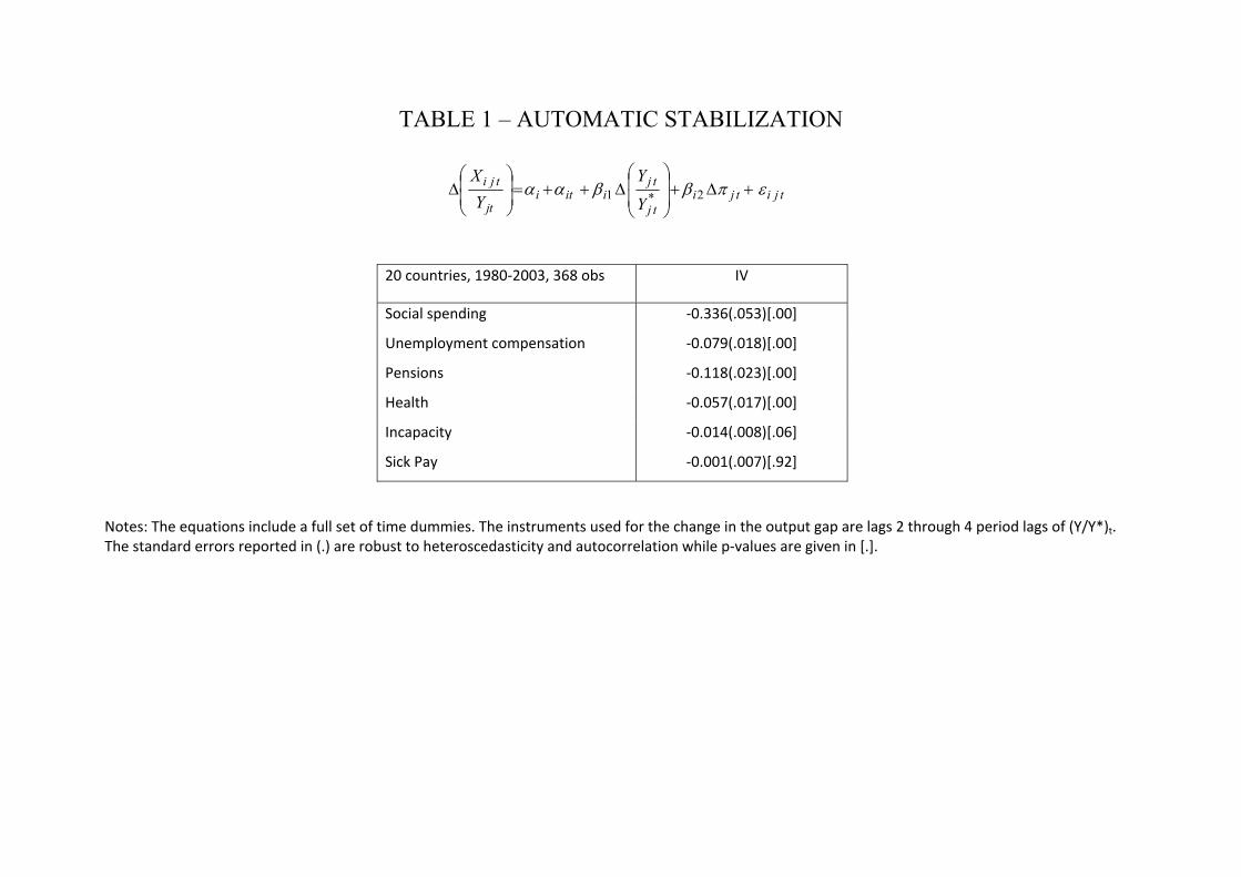
TABLE 1 – AUTOMATIC STABILIZATION

tjitjitj

tjiiti

tj

tji

Y

YY

Xεπββαα +Δ+

⎟⎟

⎠

⎞

⎜⎜

⎝

⎛Δ++=⎟

⎟⎠

⎞⎜⎜⎝

⎛Δ 2*1

20 countries, 1980‐2003, 368 obs  IV 

Social spending   ‐0.336(.053)[.00] 

Unemployment compensation   ‐0.079(.018)[.00] 

Pensions  ‐0.118(.023)[.00] 

Health  ‐0.057(.017)[.00] 

Incapacity  ‐0.014(.008)[.06] 

Sick Pay  ‐0.001(.007)[.92] 

Notes: The equations include a full set of time dummies. The instruments used for the change in the output gap are lags 2 through 4 period lags of (Y/Y*)t.  The standard errors reported in (.) are robust to heteroscedasticity and autocorrelation while p‐values are given in [.]. 

29

TABLE 2: AUTOMATIC AND DISCRETIONARY RESPONSES TO THE CYCLE

tjitjitj

tjitji

tj

tji

tj

tjiiti

tj

tji elecYD

Y

Y

Y

YYX

εββπβββαα ++⎟⎟⎠

⎞⎜⎜⎝

⎛+Δ+

⎟⎟

⎠

⎞

⎜⎜

⎝

⎛Δ+

⎟⎟

⎠

⎞

⎜⎜

⎝

⎛Δ++=⎟

⎟⎠

⎞⎜⎜⎝

⎛Δ

−

−

−

−5

1

143*

1

12*1

IV Estimates 

20 countries, 1982‐2003, 350obs

(A) Primary Surplus 

(B) Government  Receipts 

(C) Government Social 

Spending 

(D) Gov. Consumption 

Spending 

(E)  Gov. Investment 

Spending 

Δ(Y/Y*)t  0.301(.281)[.29]  ‐0.252(.178)[.16]  ‐0.353(.073)[.00]  ‐0.242(.069)[.00]   0.041(.085)[.63]  Δ(Y/Y*)t-1  0.431(.271)[.11]   0.354(.161)[.03]  ‐0.009(.067)[.90]   0.029(.069)[.67]  ‐0.097(.091)[.28]  Δ πt  0.010(.009)[.92]  ‐0.114(.040)[.01]  ‐0.067(.026)[.02]  ‐0.081(.028)[.00]   0.024(.038)[.52]  (D/Y)t-1  0.032(.009)[.00]   0.015(.005)[.01]  ‐0.007(.003)[.02]  ‐0.003(.003)[.21]  ‐0.008(.003)[.02]  Elec ‐0.480(.195)[.02]  ‐0.283(.122)[.02]   0.084(.061)[.17]   0.072(.057)[.21]   0.041(.088)[.64] 

Combined automatic and discretionary response (β1+ β2)

0.733(.195)[.00]  0.101(.106)[.34]  ‐0.361(.070)[.00]  ‐0.213(.054)[.00]  ‐0.057(.069)[.61] 

Endogeneity Tests χ2(1): (Y/Y*)t 0.055[.82]  0.519[.47]  2.564[.11]  0.996[.32]  0.006[.94]  (D/Y)t-1 21.01[.00]  7.869[.01]  4.571[.03]  2.092[.15]  5.798[.02] 

Joint signif. of αit F(22,321):  1.50 [.07]  2.42[.00]  1.42[.10]  2.38[.00]  1.25[.20] Underidentification test:  Kleibergen‐Paap rK LM test  

 16.13[.00] 

 16.13[.00] 

 16.13[.00] 

 16.13[.00] 

 16.13[.00] 

Over identification Restrictions: Hansen J‐test  

0.169[.92]  0.448[.80]  0.183[.91]  1.265[.53]  0.109[.95] 

Notes:  The equations include a full set of time dummies. Instruments used are lags 2‐4 of the output gap and lags 2‐3 of the change in the debt to GDP ratio. The standard errors reported in (.) are robust to heteroscedasticity and autocorrelation while P‐values are given in [.]. 

30

TABLE 3: ASYMMETRIC RESPONSES TO THE CYCLE

tjitjitj

tjitji

tj

tji

tj

tji

tj

tji

tj

tjiitii

tj

tji elecYD

YY

YY

YY

YY

YX

εββπβββββααα ++⎟⎟⎠

⎞⎜⎜⎝

⎛+Δ+⎟

⎟⎠

⎞⎜⎜⎝

⎛Δ+⎟

⎟⎠

⎞⎜⎜⎝

⎛Δ+⎟

⎟⎠

⎞⎜⎜⎝

⎛Δ+⎟

⎟⎠

⎞⎜⎜⎝

⎛Δ+++=⎟

⎟⎠

⎞⎜⎜⎝

⎛Δ

−

−

+

−

−

+

−

−+7

1

165*

1

14*3*

1

12*1

  Gov. Social Spending  Government Consumption IV,  350 obs.  (A)  (B)  (C)  (D) 

Δ(Y/Y*)t  0.310(.081)[.00]  ‐0.263(.069)[.00]  ‐0.259(.070)[.00]  ‐0.238(.058)[.00]  Δ(Y/Y*)t-1 ‐0.013(.067)[.84]   0.036(.068)[.59]   0.033(.068)[.63]  ‐‐‐  Δ(Y/Y*)+

t ‐0.182(.170)[.29]   0.021(.157)[.13]  ‐‐‐  ‐‐‐  Δ(Y/Y*)+

t-1  0.124(.190)[.51]   0.010(.152)[.66]   0.114(.129)[.38]   0.120(.126)[.34]  Δ πt ‐0.077(.023)[.00]  ‐0.088(.025)[.00]  ‐0.088(.025)[.00]  ‐0.086(.025)[.00]  (D/Y)t-1 ‐0.003(.003)[.25]  ‐0.001(.002)[.55]  ‐0.001(.002)[.55]  ‐0.001(.002)[.54]  Elec  0.077(.061)[.20]   0.078(.057)[.17]   0.077(.055)[.17]   0.078(.055)[.16] Automatic policy in ‘bad’ times:                 β1  ‐0.310(.081)[.00]  ‐0.263(.069)[.00]  ‐0.259(.070)[.00]  ‐0.238(.058)[.00] Automatic policy in ‘good’ times:        β1+β3  ‐0.492(.159)[.00]  ‐0.242(.162)[.14]  ‐0.259(.070)[.00]  ‐0.238(.058)[.00] Combined automatic &discretionary policy 

       in ‘bad’ times:    β1+β2  

‐0.324(.089)[.00]  

‐0.226(.064)[.00]  

‐0.226(.064)[.00]  

‐0.238(.058)[.00]             in ‘good’ times: β1+β2+β3+β4  ‐0.381(.124)[.00]  ‐0.105(.120)[.38]  ‐0.112(.095)[.24]  ‐0.118(.097)[.22] 

Endogeneity Tests χ2(1): (Y/Y*)t

(Y/Y*)+t

(D/Y)t-1

1.002[.32] 0.761[.38] 0.519[.47] 

0.663[.42] 0.152[.70] 0.550[.46] 

   

Joint signif. of αit :  F(22,318)=1.34[.14]  F(22,318)=1.93[.01]  F(22,319)=1.96[.01]  F(20,320)=2.03[.00] Kleibergen‐Paap rK LM Statistic   12.09[.02]  12.09[.02]  16.99[.00]  17.28[.01] Hansen J statistic   3.757[.29]  3.970[.26]  4.098[.39]  4.687[.46] Tests of joint restrictions:   

H0:α+=β3=β4=0,  F(3,318) = 0.59[.62] 

H0:α+=β3=β4=0,  F(3,318)= 0.76[.51] 

H0:α+=β4=0,  F(2,319)=1.14[.32] 

H0:α+=β4=0,  F(2,320)=2.09[.13] 

Test of reduction column (B) to (D):    H0:β2=β3=0,  F(2,318)=0.14[.87] 

   

Notes: see Table 2. 

TABLE 4: AUTOMATIC AND DISCRETIONARY RESPONSES - INTRODUCING REAL TIME DATA

31

tjitjitj

tjitji

tjr

tjri

tj

tjiiti

tj

tji elecYD

YY

YY

YX

εββπβββαα ++⎟⎟⎠

⎞⎜⎜⎝

⎛+Δ+⎟

⎟⎠

⎞⎜⎜⎝

⎛Δ+⎟

⎟⎠

⎞⎜⎜⎝

⎛Δ++=⎟

⎟⎠

⎞⎜⎜⎝

⎛Δ

−

−5

1

143*2*1

IV, 177 obs.  (A) Primary Surplus  (B) Government Receipts  (C) Government Social Spending   (D) Government Consumption 1994‐2003  Final Data  Real Time Data 

 Final Data  Real Time Data 

 Final Data  Real Time Data  Final Data  Real Time Data 

Δ(Y/Y*)t 0.568(.354)[.11]   1.081(.271)[.00]  0.023(.296)[.94]   0.297(.185)[.11]  ‐0.451(.101)[.00]  ‐0.477(.113)[.00]  ‐0.120(.087)[.17]  ‐0.217(.083)[.01] 

Δ(Y/Y*)t-1  0.512(.288)[.08]     0.318(.235)[.18]    ‐0.014(.125)[.11]     ‐0.107(.097)[.27]   

Δ(Yr/Yr*)t    ‐0.317(.113)[.01]    ‐0.119(.070)[.09]       0.034(.061)[.57]      0.048(.042)[.26] 

Δπt ‐0.002(.131)[.99]  ‐0.016(.123)[.90]  ‐0.125(.066)[.06]  ‐0.132(.059)[.03]  ‐0.079(.033)[.02]  ‐0.077(.034)[.03]  ‐0.123(.024)[.00]  ‐0.120(.022)[.00] 

(D/Y)t-1  0.024(.012)[.04]   0.019(.011)[.08]   0.016(.008)[.03]   0.012(.006)[.06]  ‐0.004(.005)[.36]  ‐0.004(.004)[.31]  ‐0.001(.034)[.73]  ‐0.002(.003)[.40] 

Elec ‐0.277(.273)[.31]  ‐0.534(.235)[.02]  ‐0.041(.219)[.85]  ‐0.188(.159)[.24]    0.129(.107)[.23]  ‐0.140(.097)[.15]  ‐0.001(.079)[.99]   0.050(.064)[.78] 

Combined response β1+ β2 1.080(.294)[.00]  0.764(.244)[.00]  0.341(.195)[.08]  0.178(.171)[.30]  ‐0.495(.072)[.00]  ‐0.443(.083)[.00]  ‐0.326(.064)[.00]  ‐0.169(.067)[.01] 

Endog.tests: Δ(Y/Y*)t (D/Y)t-1

1.584[.21] 6.827[.01] 

7.854[.01] 4.371[.04] 

0.277[.60] 4.703[.03] 

1.518[.22] 2.980[.08] 

6.193[.01] 0.876[.35] 

4.131[.04] 1.502[.22] 

0.001[.98] 0.183[.67] 

0.627[.10] 0.008[.93] 

Joint significance of αit F(9,162)

3.12[.00]  3.92[.00]  3.41[.00]  3.67[.00]  1.14[.33]  1.33[.22]  3.38[.00]  3.50[.00] 

Kleibergen‐Paap LM   7.315[.06]  7.624[.11]  7.315[.06]  7.624[.11]  7.315[.06]  7.624[.11]  7.315[.06]  7.624[.11] Hansen J‐test  0.668[.71]  2.420[.49]  0.495[.78]  3.317[.35]  2.898[.25]  3.006[.39]  5.323[.07]  6.266[.10] 

Notes: See Table 2.  Real time output gaps are not instrumented. 

32

TABLE A1: ARE EMU COUNTRIES DIFFERENT? – SOCIAL SPENDING

tjitjitj

tjitjiEMU

tj

tjiEMU

tj

tji

tj

tji

tj

tjiitEMUiiti

tj

tji elecYD

DYY

DYY

YY

YY

DYX

εββπβββββμαα ++⎟⎟⎠

⎞⎜⎜⎝

⎛+Δ+⎟

⎟⎠

⎞⎜⎜⎝

⎛Δ+⎟

⎟⎠

⎞⎜⎜⎝

⎛Δ+⎟

⎟⎠

⎞⎜⎜⎝

⎛Δ+⎟

⎟⎠

⎞⎜⎜⎝

⎛Δ+++=⎟

⎟⎠

⎞⎜⎜⎝

⎛Δ

−

−

−

−

−

−7

1

165*

1

14*3*

1

12*1

Notes: See Table 2.  

IV estimates 20 countries, 1982‐2003, n=350 

Government Social Spending 

(i) (As Table 2) 

 

Government Social Spending 

(ii) 

Δ(Y/Y*)t ‐0.353(.073)[.00]  ‐0.243(.073)[.00]  Δ(Y/Y*)t-1 ‐0.009(.067)[.90]  ‐0.097(.075)[.20]  Δ(Y/Y*)t..DEMU ‐‐  ‐0.302(.105)[.00]  Δ(Y/Y*)t-1.DEMU ‐‐         0.227(.107)[.04]  Δ πt ‐0.067(.026)[.02]  ‐0.080(.025)[.00]  (D/Y)t-1 ‐0.007(.003)[.01]  ‐0.007(.004)[.06]  Elec  0.084(.061)[.17]   0.037(.064)[.56] 

Combined response all countries β1 + β2 Combined response non EMU countries  β1 + β2

Contemporaneous response EMU countries β1 + β3 Combined response EMU countries β1 + β2+ β3 + β4

‐0.361(.070)[.00] ‐‐ ‐‐ ‐‐ 

‐‐ ‐0.341(.074)[.00] ‐0.546(.098)[.00] ‐0.416(.086)[.00] 

Joint significance of DEMU terms γ, β3 and β4 ‐‐  F(3,318)=2.81[.04] 

Joint significance of αit  F(22,321)=1.42[.10]  F(22,318)=1.53[.04] 

Underidentification test: Kleibergen‐Paap LM test  16.13[.00]  17.36[.00] 

Over identification Restrictions: Hansen J‐test   0.183[.91]  0.704[.87] 

REFERENCES

Aghion, Philippe and Ioana Marinescu (2007). “Cyclical budgetary policy and economic growth: What do we learn from OECD panel data?” NBER Macroeconomics Annual, Vol. 22.

Alesina, Alberto and Silvia Ardagna (2010). “Large changes in fiscal policy: Taxes versus spending,” in Jeffrey Brown, ed., Tax Policy and the Economy, vol. 24, NBER.

Alesina, Alberto, Silvia Ardagna, Roberto Perotti and Fabio Schiantarelli (2002). “Fiscal policy, profits, and investment,” American Economic Review, 92, 571-589.

Alesina, Alberto and Robert Perotti (1995). “Fiscal expansions and adjustments in OECD countries,” Economic Policy, 21, 205-48.

Annett, Anthony (2006). “Enforcement and the Stability and Growth Pact: How fiscal policy did and did not change under Europe’s fiscal framework,” IMF Working Paper WP/06/116.

Armingeon, Klaus, Marlène Gerber, Philipp Leimgruber, and Michelle Beyeler (2008). Comparative Political Data Set 1960-2006, Institute of Political Science, University of Berne.

Arreaza, Adriana, Bent Sørensen, and Oved Yosha (1999). “Consumption smoothing through fiscal policy in OECD and EU countries,” in James Poterba and Jürgen von Hagen, eds., Fiscal Institutions and Fiscal Performance, Chicago: University of Chicago Press, 59-80.

Balassone, Fabrizio and Mauro Francese (2004). “Cyclical asymmetry in fiscal policy, debt accumulation, and the Treaty of Maastricht,” Banca d’Italia Temi di Discussione no. 531.

Balassone, Fabrizio, Mauro Francese and Stefania Zotteri (2008). “Cyclical asymmetry in fiscal variables,” Banca d’Italia Temi di Discussione no. 671.

Ballabriga, Fernando and Carlos Martinez-Mongay (2002). “Has EMU shifted policy?” European Commission, Director-General for Economic and Financial Affairs, Economic Paper no. 166.

Baum, Christopher, Mark Schaffer and Steven Stillman, (2010), IVREG2: Stata module for extended instrumental variables/2SLS and GMM estimation, Statistical Software Components, Boston College, http://econpapers.repec.org/RePEc:boc:bocode:s425401.

Beetsma, Roel and Massimo Giuliodori (2008). “Fiscal adjustment to cyclical developments in the OECD: An empirical analysis based on real-time data,” CEPR Discussion Paper No. 6692.

Beetsma, Roel and Massimo Giuliodori (2010). “Discretionary fiscal policy: Review and estimates for the EU,” CESifo Working Paper No. 2948.

Bernoth, Kerstin, Andrew Hughes Hallett and John Lewis (2007), “Did fiscal policymakers know what they are doing? CEPR Discussion Paper no. 6758.

Blanchard, Olivier (1990). “Suggestions for a new set of fiscal indicators,” OECD Economics Department Working Paper No. 79.

Blanchard, Olivier and Roberto Perotti (2002). “An empirical characterization of the dynamic effects of change in government spending and taxes on output,” Quarterly Journal of Economics, 117(4), 1329-1368.

Bohn, Henning (1998). “The behavior of U.S. public debt and deficits,” Quarterly Journal of Economics, 113(3), 949-963.

Bohn, Henning (2005). “The sustainability of fiscal policy in the United States,” University of California at Santa Barbara, mimeo.

Bun, M.J.G. and Jan Kiviet (2006). “The effects of dynamic feedbacks on LS and MM estimator accuracy in panel data models,” Journal of Econometrics 132, 409-444.

Buti, Marco and André Sapir, eds. (1998). Economic Policy in EMU: A Study by the European Commission Services, Oxford: Clarendon Press.

34

Candelon, Bertrand, Joan Muysken and Robert Vermeulen (2010). “Fiscal policy and monetary integration in Europe: An update,” Oxford Economic Papers, 62(2), 323-349.

Celasun, Oya, Xavier Lebrun and Jonathan Ostry (2007). Primary surplus behavior and risks to fiscal sustainability in emerging market countries: A “Fan-chart” approach, IMF Staff Papers, 53(3), 401-425.

Cameron, Colin and Pravin Trivedi (2005). Microeconomics: Methods and Applications, Cambridge University Press.

Cimadomo, Jacopo (2007). “Fiscal policy in real time,” CEPII Working Paper no. 2007-10. Darby, Julia and Jacques Melitz (2008). “Social spending and automatic stabilisers in the

OECD,” Economic Policy, 56, October, 715-756. De Haan, Jakob, Jan-Egberg Sturm, and Geert Beikhuis (1999).”The weak government thesis:

Some new evidence,” Public Choice, 101, 163-176. Fatas, Antonio and Ilian Mihov (2003a). “On constraining fiscal policy discretion in EMU,”

Oxford Review of Economic Policy, 19, 112-31. Fatas, Antonio and Ilian Mihov (2003b). “The case for restricting fiscal policy discretion,”

Quarterly Journal of Economics, 118, 1419-1447. Forni, Lorenzo and Sandro Momigliano (2005). “Cyclical sensitivity of fiscal policies based

on real-time data,” Applied Economics Quarterly, 50(3), 299-326. Galí, Jordi and Roberto Perotti (2003). “Fiscal policy and monetary integration in Europe,”

Economic Policy, 37, October, 533-572. Gerdtham, Ulf-G. and Christopher Ruhm (2006). “Deaths rise in good economic times:

Evidence from the OECD,” Economics and Human Biology, 4(3), 298-316. Giuliodori, Massimo and Roel Beetsma (2008). “On the relationship between fiscal plans in

the European Union: An empirical analysis based on real-time data,” Journal of Comparative Economics, 36, 221-242.

Golinelli, Roberto and Sandro Momigliano (2006). “Real-time determinants of fiscal policies in euro area,” Journal of Policy Modeling, 28, 943-964.

Golinelli, Roberto and Sandro Momigliano (2009). “The cyclical reaction of fiscal policies in the Euro area: The role of modelling choices and data vintages,” Fiscal Studies, 30(1), 39-72.

Grilli, Vittorio, Donato Masciandro and Guido Tabellini (1991). “Political and monetary institutions ad public financial policies in the industrial countries,” Economic Policy, 13, 341-392.

von Hagen, Jürgen and Ian Harden (1995). “Budget processes and commitment to fiscal discipline,” European Economic Review, 39(3-4), 771-779.

von Hagen, Jürgen, Andrew Hughes Hallett and Rolf Strauch (2000). Budgetary Consolidation in EMU, CEPR.

Hallerberg, Mark and Jürgen von Hagen (1999). “Electoral institutions, cabinet negotiations, and budget deficits in the European Union,” in James Poterba and Jürgen von Hagen, eds., Fiscal Institutions and Fiscal Performance, Chicago: University of Chicago Press.

Hercovitz, Zvi and Michel Strawczynski (2004). “Cyclical ratcheting in government spending: Evidence from the OECD,” Review of Economics and Statistics, 86(1), 353-361.

Hercovitz, Zvi and Michel Strawczynski (2005). “Government-spending adjustment: the OECD since the nineties,” Banca d’Italia Annual Conference on Public Expenditure, 809-826.

International Monetary Fund (2001). “Fiscal policy and macroeconomic stability,” World Economic Outlook, May.

International Monetary Fund (2010). “Will it hurt? Macroeconomic effects of fiscal consolidation,” World Economic Outlook, October, chapter 3.

35

Jonung, Lars and Martin Larch (2006). “Improving fiscal policy in the EU: the case for independent forecasts,” Economic Policy 47, July, 491-534.

Kalckreuth, Ulf von and Guntram Wolff (2007). “Testing for contemporary fiscal discretion with real time data,” Deutsche Bundesbank Discussion Paper Series 1: Economic Studies, no. 24.

Kontopoulos, Yianos and Roberto Perotti (1999). “Government fragmentation and fiscal policy outocomes: Evidence from the OECD,” in James Poterba and Jürgen von Hagen, eds., Fiscal Institutions and Fiscal Performance, Chicago: University of Chicago Press.

Lane, Philip (2003). “The cyclical behaviour of fiscal policy: Evidence from the OECD,” Journal of Public Economics, 87(12), 2661-2675.

Mélitz, Jacques (1997). “Some cross-country evidence about debts, deficits and the behavior of monetary and Fiscal authorities,” CEPR Discussion Papers no. 1653.

Mendoza, Enrique and Jonathan Ostry (2007). “International evidence of fiscal solvency: Is fiscal policy ‘responsible’?” NBER Working Paper 12947.

Nickell, Stephen (1981). “Biases in dynamic models with fixed effects,” Econometrica 49, 1417-1426.

Organization for Economic Cooperation and Development (2005). Economic Survey: Euro Area.

Poplawski Ribeiro, Marcos (2009). “New evidence on the effectiveness of Europe’s fiscal restrictions,” CEPII Document de Travail no. 2009-13, July.

Romer, Christina and David Romer (2009). “A narrative analysis of postwar tax changes,” University of California at Berkeley working paper, available at http://elsa.edu/~dromer /papers/nadraft609.pdf.

Romer, Christina and David Romer (2010). “The macroeconomic effects of tax changes: Estimates based on a new measure of fiscal shocks,” American Economic Review 100, no. 3, 763-801.

Roodman, David (2003) “"XTABOND2: Stata module to extend xtabond dynamic panel data estimator”, Statistical Software Components S435901, Boston College, revised 20 Apr 2010.

Roodman, David (2009). “How to do xtabond2: An introduction to difference and system GMM in Stata,” The Stata Journal, 9:1, 86-136.

Roubini, Nouriel and Jeffrey Sachs (1989). “Political and economic determinants of budget deficits in the industrial democracies,” European Economic Review, 33, 903-938.

Velasco, Andres (1999). “A model of endogenous fiscal deficits and delayed fiscal reforms,” in James Poterba and Jürgen von Hagen, eds., Fiscal Institutions and Fiscal Performance, Chicago: University of Chicago Press.