STRATEGIES OF COORDINATED CONTROL OF PSS AND POD IN …

0

University of the Andes

School of Engineering

Department of Electrical Engineering and Electronics

Master Thesis in Electrical Engineering

STRATEGIES OF COORDINATED CONTROL OF PSS AND POD

IN FACTS FOR POWER SYSTEMS.

By

José David Herrera Martinez

Under the supervision of

Mario Alberto Ríos Mesías, PhD.

Jury

Gustavo Ramos López

Álvaro Chavarro Leal

May 2016

ii

AKCNOWLEDGMENTS

I would first like to thank my thesis advisor Prof. Mario A. Ríos M. of the School of

Engineering, Department of Electrical Engineering and Electronics at Universidad de los

Andes. The door to Prof. Ríos office was always open whenever I ran into a trouble spot or

had a question about my research. Thanks for your guidance and shared knowledge during

this master thesis.

I would like to thank Colciencias and Universidad de los Andes for their support for the

development of this work, under the program “Jovenes Investigadores 2014, convocatoria

645 de 2014”. Thanks for the Scholarship.

Finally, I must express my very profound gratitude to my parents for providing me with

unfailing support and continuous encouragement throughout my years of study and through

the process of researching and writing this thesis. This accomplishment would not have

been possible without them. Thank you.

iii

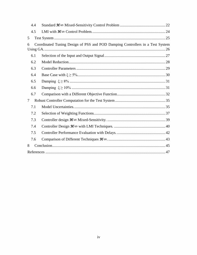
CONTENTS

Akcnowledgments .................................................................................................................. ii

Abstract ................................................................................................................................... v

List of Tables ......................................................................................................................... vi

List of Figures ....................................................................................................................... vii

1 Introduction ..................................................................................................................... 1

1.1 Problem Background ............................................................................................... 1

1.2 Objectives ................................................................................................................ 1

1.2.1 General.............................................................................................................. 1

1.2.2 Specific ............................................................................................................. 1

1.3 Scope ........................................................................................................................ 2

1.4 Organization of the Thesis ....................................................................................... 2

2 Power System Stabilizer: An Overview .......................................................................... 4

2.1 Power System Stabilizer .......................................................................................... 4

2.1.1 Design Considerations ...................................................................................... 5

2.1.2 PSS Input Signal ............................................................................................... 5

2.1.3 Methods of PSS Design .................................................................................... 6

2.1.4 Advantages and Disadvantages ........................................................................ 9

2.2 Power Oscillation Damping ................................................................................... 10

2.3 Coordination of PSS and POD ............................................................................... 10

2.4 Robust Controller ................................................................................................... 11

2.5 Time delays in Power System ................................................................................ 11

3 Coordinated Design of PSS and POD damping Controllers ......................................... 13

3.1 Analysis Modal ...................................................................................................... 14

3.1.1 Selection of the PSS and POD Controller Input Signal ................................. 15

3.2 Model Reduction .................................................................................................... 15

3.3 Optimization Problem Formulation ....................................................................... 17

3.4 Genetic Algorithm Optimization Technique ......................................................... 17

4 Robust Controller Design .............................................................................................. 19

4.1 System Mathematical Modelling ........................................................................... 19

4.2 Model Uncertainties ............................................................................................... 20

4.3 Selection of Weighting Functions .......................................................................... 21

iv

4.4 Standard 𝓗∞ Mixed-Sensitivity Control Problem ............................................... 22

4.5 LMI with 𝓗∞ Control Problem. ........................................................................... 24

5 Test System ................................................................................................................... 25

6 Coordinated Tuning Design of PSS and POD Damping Controllers in a Test System

Using GA. ............................................................................................................................. 26

6.1 Selection of the Input and Output Signal ............................................................... 27

6.2 Model Reduction .................................................................................................... 28

6.3 Controller Parameters ............................................................................................ 29

6.4 Base Case with ξ ≥ 5%........................................................................................... 30

6.5 Damping ξ ≥ 8% ................................................................................................... 31

6.6 Damping ξ ≥ 10% ................................................................................................. 31

6.7 Comparison with a Different Objective Function .................................................. 32

7 Robust Controller Computation for the Test System .................................................... 35

7.1 Model Uncertainties. .............................................................................................. 35

7.2 Selection of Weighting Functions. ......................................................................... 37

7.3 Controller design 𝓗∞ Mixed-Sensitivity. ............................................................ 39

7.4 Controller Design 𝓗∞ with LMI Techniques. ..................................................... 40

7.5 Controller Performance Evaluation with Delays. .................................................. 42

7.6 Comparison of Different Techniques 𝓗∞. ........................................................... 43

8 Conclusion ..................................................................................................................... 45

References ............................................................................................................................ 47

v

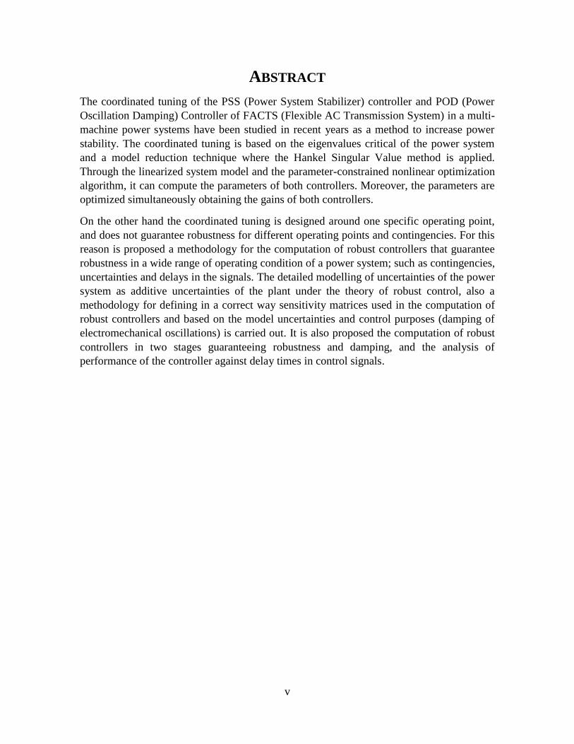
ABSTRACT

The coordinated tuning of the PSS (Power System Stabilizer) controller and POD (Power

Oscillation Damping) Controller of FACTS (Flexible AC Transmission System) in a multi-

machine power systems have been studied in recent years as a method to increase power

stability. The coordinated tuning is based on the eigenvalues critical of the power system

and a model reduction technique where the Hankel Singular Value method is applied.

Through the linearized system model and the parameter-constrained nonlinear optimization

algorithm, it can compute the parameters of both controllers. Moreover, the parameters are

optimized simultaneously obtaining the gains of both controllers.

On the other hand the coordinated tuning is designed around one specific operating point,

and does not guarantee robustness for different operating points and contingencies. For this

reason is proposed a methodology for the computation of robust controllers that guarantee

robustness in a wide range of operating condition of a power system; such as contingencies,

uncertainties and delays in the signals. The detailed modelling of uncertainties of the power

system as additive uncertainties of the plant under the theory of robust control, also a

methodology for defining in a correct way sensitivity matrices used in the computation of

robust controllers and based on the model uncertainties and control purposes (damping of

electromechanical oscillations) is carried out. It is also proposed the computation of robust

controllers in two stages guaranteeing robustness and damping, and the analysis of

performance of the controller against delay times in control signals.

vi

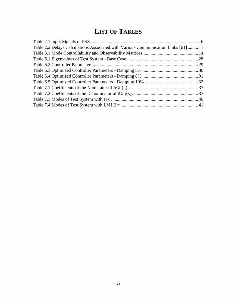
LIST OF TABLES

Table 2.1 Input Signals of PSS ............................................................................................... 6

Table 2.2 Delays Calculations Associated with Various Communication Links [61] ......... 11

Table 3.1 Mode Controllability and Observability Matrices ................................................ 14

Table 6.1 Eigenvalues of Test System - Base Case .............................................................. 28

Table 6.2 Controller Parameters ........................................................................................... 29

Table 6.3 Optimized Controller Parameters - Damping 5% ................................................ 30

Table 6.4 Optimized Controller Parameters - Damping 8% ................................................ 31

Table 6.5 Optimized Controller Parameters - Damping 10% .............................................. 32

Table 7.1 Coefficients of the Numerator of ∆Gij(s) ............................................................. 37

Table 7.2 Coefficients of the Denominator of ∆Gij(s) ......................................................... 37

Table 7.3 Modes of Test System with H∞ ........................................................................... 40

Table 7.4 Modes of Test System with LMI H∞ ................................................................... 41

vii

LIST OF FIGURES

Figure 2.1 Methods of Power System Stabilizer Design. ....................................................... 6

Figure 3.1 Block Diagram Representation PSS [1] .............................................................. 13

Figure 3.2 Block Diagram Representation POD [1]............................................................. 14

Figure 3.3 Flow Chart of the Optimization Coordinated Tuning ......................................... 18

Figure 4.1 General control problem formulation without uncertainty [53], [55] ................. 19

Figure 4.2 The additive and multiplicative uncertainty [72], [80]-[81]. .............................. 20

Figure 4.3 Typical H∞ Mixed Sensitivity Optimization with Additive Uncertainty. .......... 22

Figure 5.1 Kundur's Four-Machine Two-Area Modified with SVC [1]. ............................. 25

Figure 6.1 Selection of Input and Output Signals for the Linearization of Test System. .... 26

Figure 6.2 Test System with the PSS and POD Controllers. ................................................ 27

Figure 6.3 Active Power Flow Through Interconnection of Area 1 to Area 2 - Without

Supplementary Control. ........................................................................................................ 28

Figure 6.4 Frequency of the Original and the Reduced 18th Order System ........................ 29

Figure 6.5 Diagram of Poles and Zeros Base Case .............................................................. 30

Figure 6.6 Diagram of Poles and Zeros with ξ ≥ 8%. .......................................................... 31

Figure 6.7 Diagram of Poles and Zeros with ξ ≥ 10%. ........................................................ 32

Figure 6.8 Active Power Flow Through Interconnection of Area 1 to Area 2 – with

Supplementary Control. ........................................................................................................ 33

Figure 6.9 Power Generation - Generator 2. ........................................................................ 33

Figure 6.10 Frequency Behavior - Generator 2. ................................................................... 34

Figure 6.11 SVC Bus Voltage Behavior. ............................................................................. 34

Figure 7.1 Test System with the Robust Controller. ............................................................ 35

Figure 7.2 Model Uncertainties and Upper Bound............................................................... 36

Figure 7.3 Largest Model Uncertainty. ................................................................................ 36

Figure 7.4 Frequency Response of the Inverse of W1 ......................................................... 38

Figure 7.5 Frequency Response of the Inverse of W3 ......................................................... 39

Figure 7.6 Active Power Flow Through the Area 1 to Area 2 After the H∞ Controller. ..... 40

Figure 7.7 Active Power Flow Through the Area 1 to Area 2 After the H∞ Controller with

LMI. ...................................................................................................................................... 41

Figure 7.8 Test System with Delay Signals. ......................................................................... 42

Figure 7.9 Active Power Flow Through the Area 1 to Area 2 with Delay Signals. ............. 43

Figure 7.10 Power Generation – Generator 2. ...................................................................... 43

Figure 7.11 Frequency Response – Generator 2................................................................... 44

Figure 7.12 SVC Bus Voltage Behavior. ............................................................................. 44

1

1 INTRODUCTION

1.1 PROBLEM BACKGROUND

The stability of the power system is one of the most important aspect in the operation and

safety of electrical systems, as it refers to the ability of the system to reach a steady state

after a disturbance [1].

Once electric power systems are developed in an interconnected form in which spontaneous

oscillations at low frequencies in order of 0.1 to 3 Hz could be presented [2]. These

oscillations are caused by faults, increases in charges, lost control, small changes in the

reference voltage regulator automatic voltage (AVR), among others. Such fluctuations tend

to stay for a long time and in some cases tend to grow, causing the separation of power

systems if there is not adequate damping. Moreover, low frequency oscillations cause

limitations on the ability to transfer power, preventing transmission lines operating at

maximum capacity [1], [2].

Generally, some generators are provided with an additional control that are power system

stabilizers (PSS) which provides additional damping to oscillations of the generator rotor

through auxiliary signs of stabilization. On the other hand flexible ac transmission system

(FACTS) can be used to improve system stability by means of a supplementary control

signal for power oscillation damping (POD) [1], [3]. However, not coordination of local

control in the PSS and POD could cause destabilizing interactions in the power system

when both are present.

1.2 OBJECTIVES

1.2.1 GENERAL

Apply different methodologies of control under wide area measurement system (WAMS),

such that it allows to develop damping controllers to the phenomena of electromechanical

oscillations implementing in operational areas and coordinated properly.

1.2.2 SPECIFIC

Implement a methodology that allows to identify or select generators and FACTS devices

of the power system, where it can be installed supplementary controllers for the damping of

electromechanical oscillations, so that:

The optimal locate and appropriate number of PSSs and PODs is determinate.

The coordinated tuning of both controllers PSS and POD in the power system,

through optimization algorithms.

The implementation of centralize robust controllers that add damping to the

generators and FACTS device.

2

The analysis of signal delays in the schemes of robust controllers.

1.3 SCOPE

The methodologies that are developed will be applied to a test system, which is based on

the Kundur power system [1], [4], the implementation is performed in the software

MATLAB-Simulink using the library SimPower, the Kundur power system is modified by

adding an SVC FATCS device in the middle of the interconnected areas.

1.4 ORGANIZATION OF THE THESIS

This thesis is organized into 8 chapters

Chapter 1

This chapter gives an outline of the thesis, and determines the objectives and scope of the

project.

Chapter 2

This chapter reviews the published material on the objective of the thesis, and discusses a

brief introduction about PSS background, the POD controller, and the robust controller.

Chapter 3

This chapter presents a methodology to make a coordinated tuning design of PSS and POD

damping controller using a genetic algorithm.

Chapter 4

This chapter presents a methodology to model an additive uncertainty, and select an

adequate weighting matrix for multi input multi output system. Also a robust control theory

is presented to compute the ℋ∞ mixed-sensitivity control and the LMI constraint applied to

the ℋ∞ optimal control.

Chapter 5

This chapter shows the test system in which the strategies of coordinated control are

applied.

Chapter 6

This chapter presents simulation results of the test system, applying the coordinated tuning

of PSS and POD damping controllers using a genetic algorithm.

Chapter 7

This chapter presents simulation results of the test system, applying the robust controller

centralized using the standard and LMI techniques based on ℋ∞- norm.

3

Chapter 8

This chapter concludes the thesis.

4

2 POWER SYSTEM STABILIZER: AN OVERVIEW

At the late 1950’s most of the new generator units were equipped with automatic regulator

voltages (AVR). As these units were taking a higher penetration in the power system, it

caused a negative impact on the dynamic stability by the action of the AVR [5]. Sudden

oscillations were presented, several of these in small magnitude and low frequency, leading

to the power system to operate in different conditions, as limit the power transfer or load

shedding. The problem encouraged many researchers to develop an electrical device that

aid in damping these oscillations. The power system stabilizer (PSS), initially called

supplementary control systems, were developed in the mid 1960’s in response to power

system operations in the Pacific Intertie [1], [2], [6]. The oscillations presented in the power

system occurred at low frequencies (< 1 Hz), were lightly damped, and became known as

inter-area modes. The term inter-area is used because the active power oscillations were

observed between the Pacific Northwest and the Southwest [6], [7]. The oscillations are

comprised of combinations of many generators on one part of the system (Northwest)

swinging against generators on another part of the system (Southwest). This situation

developed slowly as the stability margins were reduced when electrical systems were

interconnected together and power was transmitted from one region to another. With the

introduction and utilization of high gain fast acting excitation systems for system transient

stability, inter-area oscillations became more pronounced [6], [7].

The first applications of the PSSs were developed and installed in the 1960’s in the United

States on the Western Systems [5]. These applications used electronics filters, amplifiers,

and analog controllers to damp generator electromechanical oscillations in order to protect

the shaft line and stabilize the network.

The PSS was evolving, the conventional PSS was split into analog and digital, being the

last designed in software through a computer. With the time, the PSS changes to dual-input

singles [8], which is designed by using combinations of power and speed or frequency as

stabilizing singles. Nowadays, many companies as ABB, SIEMENS, MITSUBISHI

ELECTRIC, GENERAL ELECTRIC, among others, have developed several applications

as Integral accelerating PSS, Adaptive PSS, Multi-Band PSS [9]-[11], which permits to the

PSS operates over an entire generating range.

Today, many generators are equipped with a PSS, as these PSS became a larger percentage

in the generating units, the complex of tune is hard. Thus, correct tuning of the PSS

becomes critical today. Indeed, this thesis focuses on the coordination of local controllers

as are the PSS and POD, also in the implementation of the selection of weighting function,

in order to design a robust controller for generators and FACTS devices.

2.1 POWER SYSTEM STABILIZER

The basic function of PSS is to add a supplementary signal to the excitation system that

creates damping torque, which is in phase with the rotor oscillations [1], [2], [5]. The PSS

5

is a feedback controller, and from the viewpoint of classical control theory, the design of

the power system stabilizer implies the modification of the power system, in order to

introduce an additional part of the control system for a synchronous generator. The PSS is

formed by different block functions, as part of the power system stabilizer: a gain, a

washout, and a phase compensation lead-lag [1], [2], [5]. Each block has a specific

function. The gain will be selected to damp out the unstable modes properly [1], [2], [5].

The washout is a high-pass filter, so as to allow passing the rotor oscillation frequencies of

interest [1], [2], [5]. The phase compensation lead-lag compensates the phase difference

between the excitation system input and the resulting electrical toque [1], [2], [5]. Finally, a

limiter is used to keep the PSS output voltage within a range of values [1], [2], [5].

2.1.1 DESIGN CONSIDERATIONS

The main objective of the PSS is to damp out the rotor oscillations, it can influence on

power system transient stability. The action of the controller allows regulating the field

voltage of the generator through of AVR output [12]. This action produces a swing in the

AVR output. To maintain an acceptable swing in the AVR output the power system

stabilizer gain is chosen so that the resultant gain margin be small. The swing can be

reduced by the adjusting to the time constant of the washout filter [12]. Another important

aspect of the PSS is the interaction with other controls during the operation of the power

system such as FACTS devices. Also the input signals are an important aspect in the design

of the PSS, since can contain high frequencies when the oscillations occurs. Depending on

the types of plants as hydraulic or thermal, the phase compensation lead-lag can be large or

small to compensate the input signals. The most important thing is that the PSS does not

have a methodology of design and the selection criteria are arbitrary and can vary according

to the power system model.

2.1.2 PSS INPUT SIGNAL

The power system stabilizer models have been designed using various state variables such

as speed, frequency, electrical power, speed deviation, et al. The most important are

described:

Stabilizer based on Speed

The PSS based on speed uses the rotor shaft speed as an input signal to compensate for the

lags in the transfer function, in order to produce a damping torque in phase with speed

changes. The main problem of this signal is the noise presents in the measure due to the

side shift of the rotor shaft [1], [5], [13].

Stabilizer based on Frequency

The PSS based on frequency uses the frequency of the output voltage of the connecting bus

as an input signal. The sensitivity of the frequency signal has an increase associated with

the rotor oscillations, this is a problem when the power system is weak, because the

stabilizer has to compensate for the reduction in the gain [1], [5], [13].

6

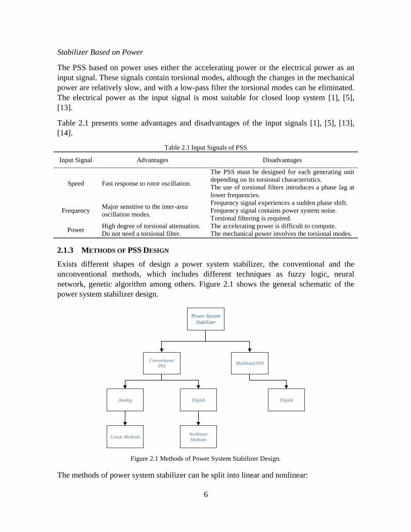
Stabilizer Based on Power

The PSS based on power uses either the accelerating power or the electrical power as an

input signal. These signals contain torsional modes, although the changes in the mechanical

power are relatively slow, and with a low-pass filter the torsional modes can be eliminated.

The electrical power as the input signal is most suitable for closed loop system [1], [5],

[13].

Table 2.1 presents some advantages and disadvantages of the input signals [1], [5], [13],

[14].

Table 2.1 Input Signals of PSS

Input Signal Advantages Disadvantages

Speed Fast response to rotor oscillation.

The PSS must be designed for each generating unit

depending on its torsional characteristics.

The use of torsional filters introduces a phase lag at

lower frequencies.

Frequency Major sensitive to the inter-area

oscillation modes.

Frequency signal experiences a sudden phase shift.

Frequency signal contains power system noise.

Torsional filtering is required.

Power High degree of torsional attenuation.

Do not need a torsional filter.

The accelerating power is difficult to compute.

The mechanical power involves the torsional modes.

2.1.3 METHODS OF PSS DESIGN

Exists different shapes of design a power system stabilizer, the conventional and the

unconventional methods, which includes different techniques as fuzzy logic, neural

network, genetic algorithm among others. Figure 2.1 shows the general schematic of the

power system stabilizer design.

Figure 2.1 Methods of Power System Stabilizer Design.

The methods of power system stabilizer can be split into linear and nonlinear:

Power System

Stabilizer

Conventional

PSSMultiband PSS

Analog

Linear MethodsNonlinear

Methods

Digital Digital

7

The linear methods are

1) Output feedback controllers

A linear method is applied in [15], the controller design is based on quantities easily

measured at the synchronous generator location, this method is presented for power

system equipped with fast-acting excitation systems.

2) Pole-shifting technique

The design of a self-tuning power system stabilizer using the pole-shifting

technique is presented in [16]. The controller uses a state feedback law 𝑢(𝑘), whose

gains are evaluated from the pole-shifting factor 𝛼. Additionally, a method for

shifting the real parts of the complex open-loop poles to any desired position,

whereas preserving the imaginary parts is presented in [17].

3) Pole-placement technique

The design of nonswitching controllers for systems with multiple operating

conditions is presented in [18]. The design of the controller is based on pole-

placement procedure, the controller 𝐻 can be found such that the eigenvalues of the

closed-loop system are stable. A new approach of pole-placement is developed in

[19]. The general procedure of pole-placement PSS design is to find the unstable

modes using participation factor analyses, it varies the damping factors one at a time

while keeping the others constant.

4) Linear Quadratic Gaussian

The design of PSS using linear quadratic gaussian regulator methodology with loop

transfer recovery (LQG/LTR) is presented in [20]. The problem is to find a

feedback control law that minimizes the quadratic performance index, associated

with weighting matrices 𝑄 and 𝑅. The controller 𝐾 is computed by Kalman

filtering.

5) Linear Quadratic Regulator

A linear optimal controller for the linearized system is presented in [21]. The PSS

controller design is based on linear quadratic regulator (LQR) as the linear

controller to simplify feedback gain design. Weighting matrices 𝑄 and 𝑅 in the

quadratic performance index are determined so that the eigenvalue of the LQR-

controlled system equals that of the conventional PSS.

6) Quantitative Feedback Theory

A robust PSS controller is designed for an uncertain power system, it is presented in

[22] and [23]. The quantitative feedback theory (QFT) procedure is as follows: the

tracking control ratio is modeled for the upper and lower bound as transfer

functions, the templates of the power system are formed for a wide range of

frequencies, the U-contour and different bounds for power system uncertainties are

determined, all the criteria are for extending the conventional stabilizer performance

to operate in a wide range.

7) Sliding mode technique

A nonlinear PSS controller is designed for a linearized system, it is presented in

[24]. The nonlinear PSS controller is based on a sliding mode controller whose

objective is to choose control signal 𝑢, to make 𝑦 (output) track 𝑦𝑑 (desired output)

8

in the presence of boundable modelling errors. The sliding mode control (SMC) has

good performance for most disturbances, but often required more energy to control.

8) Linear matrix inequalities

The design of a robust PSS controller using linear matrix inequalities (LMI) is

presented in [25]. The conventional PSS is expressed by the space state equations,

using the canonical observability form. The constrained set of LMI are formed to

minimize an optimization problem.

9) H2 norm

The design of a 𝐻2 optimal adaptive control as a power system stabilizer is

presented in [26]. The controller is used in nonlinear power systems, the optimal

control is computed by using the identified model parameters and estimated stated

by the system. The finite-horizon 𝐻2 norm minimizes the quadratic performance

index. Weighting matrices 𝑄 and 𝑅 are defined as symmetric positive semidefinite

and positive definite respectively.

10) H∞ norm

The design of a 𝐻∞ optimal control of the PSS design is presented in [27]. The

controller is based on the selection of weighting function matrices, and the nominal

power system is modelled without uncertainties.

Nonlinear Methods of design

1) Neural network

A new approach using an artificial neural network is proposed in [28]. The

parameters of the PSS are tuning in real time. The neural network is trained by a set

of input-output patterns in the training set, can yield proper PSS parameters under

any generator loading condition. Different applications were developed after, as

neural network using power flow characteristic in [29], adaptive neural network

using dynamic backpropagation in [30], et al.

2) Fuzzy Logic

The PSS controller is designed using a simple fuzzy control rules is presented in

[31]. The fuzzy control rules are constructed under the knowledge and the

experience of experts. For optimal parameters setting, a quadratic performance

index is considered and the quasi-newton method is applied [31]. The fuzzy logic

techniques allow constructing model-free controllers, different applications can be

found in [32], and [33].

3) Adaptive control

The adaptive control technique in PSS controller is presented in [34]. The adaptive

control specifies a desired performance, compute the error between the outputs of

the reference model and the actual system, and based on the correlation between this

error and the system states, update the controller gains for the system. In the

literature the adaptive control can be classified into Adaptive Automatic Methods

[35], and Heuristic Dynamic programming [36]. Nowadays, exists more

applications in adaptive control [37].

4) Genetic Algorithm

9

The design of a PSS controller based on genetic algorithm (GA) is presented in

[38]. In a genetic algorithm, a population of candidate solutions (called individuals)

to an optimization problem evolves toward better solutions, the individuals are the

parameters of the PSS controller. The technique is inspired by natural evolution,

such as selection, crossover and mutation. It generates a population of points in

each iteration. The best point of the population approaches an optimal solution.

5) Simulated Annealing

The design of a PSS controller based on simulated annealing (SA) is presented in

[39]. The SA algorithm solves an optimization problem, and search for optimal or

near optimal set of PSS parameters. The SA is derived from the physical annealing

process. This technique does not rely on the initial solution, and can ensure the

convergence to the optimal solution, starting anywhere in the search space.

6) Particle Swarm Optimization

The design of a PSS controller base on particle swarm optimization (PSO) is

presented in [40]. The PSO is a population based stochastic optimization method,

the population has 𝑛 particles that represent candidate solutions, in this case the PSS

parameters. It explores for the optimal solution from a population swarm of moving

particle vectors, based on an objective function.

7) Phasor Measurements

A new distributed-measurement technology uses the GPS and phasor measurement

units to get information on a wide-area power system. The PSS controller design is

based on the selection of appropriate control structure and then tune the stabilizer

parameters. Controller tuning is performed by minimizing a selective modal

performance index, which is presented in [41].

8) BAT optimization

The BAT algorithm is based on the echolocation behavior of microbats with varying

pulse rates of emission and loudness [42]. The objective function to design the PSS

controller, allows maximizing the damping ratio of eigenvalues, whereas the PSS

parameters are computed.

2.1.4 ADVANTAGES AND DISADVANTAGES

References [1], [2], and [43] present the advantages and disadvantages that involve the

power system stabilizer in power system:

Improve the steady-state stability limit

The steady state limit can be improved, increasing or decreasing the excitation of the

generator so that the internal field voltage is maintained, after a slow change in the load.

Increase the system positive damping

The increase of the controller gain aid to increase the damping torque, and the rotor

oscillations tend to damp out.

10

Reduced power losses

The PSS extends stability limits, increasing the generating capability of the generator and

the transfer power through the lines.

Time consuming tuning of PSS

The modulation of field voltage that damps out power and speed oscillations through

normal AVR control is performed during plant commissioning. The tuning of PSS requires

of the time to adjust the parameters.

Non-optimal damping in the entire operating range

The PSS performance must be designed to provide acceptable performance over a wide

range of system conditions, but the controller parameters are adjusted around an operating

condition (such as lines out-of-service and varying load levels).

2.2 POWER OSCILLATION DAMPING

FACTS devices are known by improving the power flow in the power system. Likewise

that the generators, the FACTS uses a supplementary control to improve damping of

electromechanical modes. The controller is known as power oscillation damping (POD), it

has the same structure of the PSS controller [44]-[46]. The main objective is to improve the

overall power system dynamic performance, and in special the damping over inter-area

modes [44]-[46].

2.3 COORDINATION OF PSS AND POD

The requirements of damping local and inter-area modes, under transient conditions have

led to coordinated the PSS and POD controllers, different approaches for the control and

tuning of the PSS and POD have been applied.

Some researchers propose a coordination between generators’ PSS and FACTS’ POD

controller devices to improve overall system performance. Some of these methods use

nonlinear complex simulations, [47] and [48] propose hybrid fuzzy controllers, and [49]

deals with an optimization problem by solving a sequential quadratic programming using

the dual algorithm.

Other methods are based on the linearization model of electric power system. The first, [49]

uses projective controls, which is expressed as a linear quadratic regulator to obtain a full-

state feedback control. The second, [50] is based on the concept of induced torque

coefficients, it proposes an optimization linear programming whose objective function

minimizes the weighted sum of the stabilizer gains. The last one designs a decentralized

multivariable excitation controller using a linear quadratic regulator [51].

11

2.4 ROBUST CONTROLLER

PSSs have been designed as additional elements or supplementary local controllers that

allow the improvement of damping and stabilization of power systems when

electromechanical problems are present. Traditionally, these PSS can be functions of lead-

lag of type analogical with fixed parameters in which the selection of its best structure and

the value of its parameters are based on simplified linear models of the power system or

computed as result of an iterative very complex process, through optimization algorithms

[28]-[42]. However, the classic control PSS is commonly designed around one specific

operating point [15]-[27], and does not guarantee robustness for different operating points

and contingencies.

Robustness has been important in control systems design, when James Watt developed his

Flyball governor in 1769. Due to its importance, the research in the robust control theory

has been developed. The different techniques provide systematic design procedures of

robust controllers for linear systems, though the extension into nonlinear cases is being

actively researched.

Exists several methods and techniques for robust controller design (LQG, 𝐻2-norm, 𝐻∞-

norm, 𝜇-synthesis), but the approach is in the ℋ∞ optimal control technique, developed in

[53], implemented in [54] and [55], using a linear matrix inequality (LMI).

2.5 TIME DELAYS IN POWER SYSTEM

Time delays in power system are associated with the communication link by which the

control signal is transmitted to the controller. These time delays have an impact on the

performance of the controller and also stability, such as, the performance of the central

controller is reduced [56]-[59].

There are several types of communication links [60], for each link exists certain ranges of

time delays [60]. Table 2.2 presents the time delay associated with each communication

link.

Table 2.2 Delays Calculations Associated with Various Communication Links [61]

Communication link

Associated delay one way (ms)

Fiber-optic cables ≈ 100 - 150

Digital microwaves links ≈ 100 - 150

Power link (PLC) ≈ 150 - 350

Telephone lines ≈ 200 - 300

Satellite link ≈ 500 - 700

The propagation delay is dependent on the medium and the physical distance separating the

individual components. The fiber-optic, power lines, and telephone lines have a

propagation delay of around 25 ms. The satellite has a propagation delay as high as 200 ms

[60].

12

13

3 COORDINATED DESIGN OF PSS AND POD DAMPING

CONTROLLERS

The conventional techniques can be used to design a controller based on an operating point,

but the designed controller usually under these techniques is complicated, and the controller

parameter values are difficult to select. In order to solve this problem, The proposed

methodology finds the coordinated tuning of gains each controllers PSS and POD placed in

generators and FACTS devices. Figures 3.1 and 3.2 show the block diagram of typical PSS

and POD used.

The values of each parameter that comprise the typical structure are:

1) 𝐾 is a general gain, it determines the amount of damping produced by the stabilizer

[1], [2], [54].

2) 𝑇𝑤 is a time constant and can assume values between 1 to 20 s ¡Error! No se

encuentra el origen de la referencia., ¡Error! No se encuentra el origen de la

referencia., ¡Error! No se encuentra el origen de la referencia., [60]. This

parameter is not critical and its value depends on the function and the modes which

will be damped ¡Error! No se encuentra el origen de la referencia., ¡Error! No

se encuentra el origen de la referencia., ¡Error! No se encuentra el origen de la

referencia., [60].

3) 𝑇1/𝑇2 and 𝑇3/𝑇4 are time constants and must be fixed to provide damping on the

frequency range where the oscillations are likely to occur ¡Error! No se encuentra

el origen de la referencia., ¡Error! No se encuentra el origen de la referencia.,

¡Error! No se encuentra el origen de la referencia., [60]. These parameters

provide a phase compensation between the power system plant and the PSS

controller, the number of the lead-lag block depend on the amount of phase

compensation that require the power system ¡Error! No se encuentra el origen de

la referencia., ¡Error! No se encuentra el origen de la referencia., [61], [62].

The frequency range of interest is 0.1 to 5Hz being the last one, the value to obtain

the maximum damping for inter-area modes ¡Error! No se encuentra el origen de

la referencia., [61], [62].

Figure 3.1 Block Diagram Representation PSS [1]

14

Figure 3.2 Block Diagram Representation POD [1]

The proposed methodology computes the gains of PSS and POD controllers simultaneously

using a genetic algorithm [62]-[64]. Chapter 3 is organized as follows: Section 3.1 Select

the input signals for modal analysis, Section 3.2 Reduce the model order for suitable control

design, Section 3.3 and 3.4 Compute the coordinated gains of PSS and POD using a genetic

algorithm.

3.1 ANALYSIS MODAL

The space state representation (1) not provided enough information with respect to which

signals must be controlled, and is necessary uses the modal space state that involves the

matrices 𝐴, 𝐵, 𝐶, 𝐷 [1].

x = Ax + Bu

y = Cx + Du (1)

Expressing (1) in terms of the transformed variables z defined by x = Φz yields

z = Λz + B′u

y = C′z + Du (2)

Where

B′ = Φ−1B

C′ = CΦ (3)

The modal matrix Λ contains in its diagonal the eigenvalues of the power system, and the

modal matrix Φ corresponds to k-th entry of the right eigenvector [1].

By inspecting B′ and C′ can be classified modes into controllable and observable,

controllable and unobservable, uncontrollable and observable, uncontrollable and

unobservable. Table 3.1 describes how can interpret this concept [1].

Table 3.1 Mode Controllability and Observability Matrices

Input/Output Signal Matrix B′ Matrix C′

0 Have no effect on the i-th mode. Have no information on the i-th

mode.

>0 Have influence to control the i-th Have information on the i-th mode.

15

mode.

3.1.1 SELECTION OF THE PSS AND POD CONTROLLER INPUT SIGNAL

The main aim is to reach the design coordinate of PSS and POD. The first step is the

selection of generators and FACTS devices where the controllers will be located. The

second step is to select the input signal to both controllers. Therefore, the linear full-order

dynamic model of the system around a nominal operating point is computed, after obtaining

the matrices of the system’s state space model, the analysis modal is made through

controllability and observability. The following are the main characteristics of a suitable

input signal:

1) The input signal should be locally measurable.

2) The electromechanical modes to be damped should be observable in the input

signal.

3) The input signal must yield correct control actions.

4) The input signal with best responses are associated with the frequency of the

machine.

3.2 MODEL REDUCTION

The behavior of a dynamic system in low frequency electromechanical oscillations ranges

from 0.1 to 3 Hz, is usually expressed as a set of nonlinear differential and algebraic (DAE)

equations of the following form ¡Error! No se encuentra el origen de la referencia.,

¡Error! No se encuentra el origen de la referencia., [66]:

�� = 𝑓(𝑥, 𝑧, 𝑢)

0 = 𝑔(𝑥, 𝑧, 𝑢)

𝑦 = ℎ(𝑥, 𝑧, 𝑢)

(4)

Where f and 𝑔 are vectors of differential and algebraic equations and ℎ is a vector of output

equations.

The nominal model system is linearized without the PSS and POD controllers, thus the

state space model is linearized around of a critical operating point and can be represented

by [65], [66], ¡Error! No se encuentra el origen de la referencia.:

x = Ax + Bu

y = Cx (5)

The order reduction technique is based on a computation algorithm of a subspace of the

product of the controllability and observability grammians using the development propose

in [66]-[68] that allows the retention of unstable modes in the reduced system.

The reduction method is applicable to multi input multiple output systems (MIMO) with

more than one input and one output signals. The advantage of developing low-order models

16

suitable for control design applications is that the computational cost is reduced and the

optimization algorithms are faster.

The Hankel Singular Values Method was used as the order reduction method. It is also

named balanced truncation, this technique is split into a group the most important states and

the least important states with poor controllability and observability.

The least important states are established based on the values that brings the Hankel

Singular Values applied to the grammians product. The Singular Value of the product of

controllability and observability grammian is 𝜎(��) = 𝑑𝑖𝑎𝑔(𝜎1, 𝜎2, … , 𝜎𝑛), thus 𝜎 are the

Hankel Singular Values (HSV) of the state space model system [65]-[68].

For stable systems, a balanced realization is an equivalent realization in which the

controllability and observability grammians are equal and diagonal, their diagonal entries

forming the vector 𝜎 of Hankel Singular Values, keeping the eigenvalues without variation.

Small entries in 𝜎 indicate states that can be removed to simplify the model.

The balanced realization in ��, is obtained by a similarity transformation:

�� ≜ 𝑃1−1𝐴𝑃1

�� ≜ 𝑃1−1𝐵

�� ≜ 𝐶𝑃1

(6)

Where 𝑃1 is the transformation matrix [66]. Under these conditions is accomplished that the

grammians of the model (𝐴, 𝐵, 𝐶) are similar and diagonal, they are computed by [65]-[68]:

�� = 𝑃1

−1𝑃𝑃1−𝑇

�� = 𝑃1𝑇𝑄𝑃1

(7)

Where 𝑃 and 𝑄 are the solutions of the system of Lyapunov equations [66]-¡Error! No se

encuentra el origen de la referencia.:

𝑃𝐴𝑇 + 𝐴𝑃 + 𝐵𝐵𝑇 = 0

𝑄𝐴 + 𝐴𝑇𝑄 + 𝐶𝑇𝐶 = 0 (8)

In (5), 𝐴, 𝐵, 𝐶 are the matrices from the continuous model in (2) linearized around the

operating point. The matrix transformation 𝑃1 which satisfies the balanced realization

definition is termed a contragredient transformation and is obtained by:

𝑃1 = 𝐿𝑝𝑉Σ−1 2⁄ (9)

Where 𝐿𝑝, 𝑉 and Σ−1 2⁄ , can be gotten using the Cholesky factors from 𝑃 and 𝑄, and the

singular values decomposition [66]-[67].

When the balanced realization is finished, the next step is truncate the new system. The

truncation algorithm is based on the Singular Values of the matrix product ��. The Hankel

Singular Values are defined above:

17

𝜎𝑖 = 𝜆𝑖(��)1 2⁄ (10)

The truncated model is then applied to obtain the reduced ignoring the least significant

states of the system model [66]-¡Error! No se encuentra el origen de la referencia.:

x = Arx + Bru

y = Crx (11)

After reducing the model, it is seen the behavior of the frequency response of both, the

original model and the reduced model, and seeing if a high accuracy in the low frequency

region from 10−1 to 101 is achieved.

3.3 OPTIMIZATION PROBLEM FORMULATION

The aim of the coordination tuning is to left-shift the electromechanical modes, while

minimizing the damping ratio. The optimization problem is formulated in (12), the

calculation is performed through the weighted sum of the objective functions:

min. 𝐽 = 𝛼 ∙ 𝜉𝑖𝑛𝑡𝑒𝑟𝑎𝑟𝑒𝑎 + 𝛽 ∙ 𝜉𝑎𝑟𝑒𝑎1 + 𝛾 ∙ 𝜉𝑎𝑟𝑒𝑎2

s.t Arx + Br = 0

𝐾𝑚𝑖𝑛 ≤ 𝐾𝑝𝑠𝑠 ≤ 𝐾𝑚𝑎𝑥

𝐾𝑚𝑖𝑛 ≤ 𝐾𝑝𝑜𝑑 ≤ 𝐾𝑚𝑎𝑥

𝜉𝑖 ≥ 5%

(12)

Where 𝛼, 𝛽 and 𝛾, correspond to the weights associated with each damping ratio 𝜉𝑖

respectively. The weights are multiples major or equal to the unit.

The constraints is the set of algebraic DAE equations in the operating point such that the

damping of each mode will be greater than a specified value (which may be different for

each mode) and the parameters of each controller as inequalities.

The mathematical formulation for damping ratio is expressed as follows [1], [2]:

𝜉𝑖 =−𝜎

√𝜎2 + 𝜔2 (13)

𝜆𝑖 = 𝜎 ± 𝑗𝜔 represents the eigenvalues of the electromechanical modes will be damped.

3.4 GENETIC ALGORITHM OPTIMIZATION TECHNIQUE

The optimization problem in (9) is a multi-objective problem, it can be posed as follows:

1) The minimization of a function that involves weighting the objective multiples

(Damping of each one of electromechanical modes that are considered).

2) Vector function of multiple damping with weighting factors.

18

The pseudocode describing the genetic algorithm is as follows:

1) Generate an initial population. 𝑡 = 0.

2) Evaluate the objective function (12), for each one of the individual.

3) Calculate fitness of each individual.

4) Apply the Selection operator over the 𝑁-individuals of the population.

5) Apply Crossover and Mutation; on the individuals selected previously.

6) Verify the stop criterion. If it is not satisfied, return to step 2, incrementing the

iteration counter 𝑡 = 𝑡 + 1, else, finishes the algorithm execution.

Figure 3.3 shows the flow chart the optimization coordinated tuning based on the genetic

algorithm.

The optimization problem formulation in this paper allows considering all the operating

points selected. The multi-objective function calculates the best gains for each controller

and also it adds damping to electromechanical modes.

Each feasible solution of the optimization problem is represented by a vector of real

numbers x = [Kpss, Kpod].

Figure 3.3 Flow Chart of the Optimization Coordinated Tuning

19

4 ROBUST CONTROLLER DESIGN

Robust control theory has a philosophy of design that is similar to the classic control, which

is based on the analysis and synthesis using frequency methods [53], [55]. The novelty of

technique of robust control is to propose methods of design that allow the synthesis of

really multivariable controllers, taking into account the uncertainty of the signal and

modelling [53], [55].

The general method of formulating control problems introduced by [53] is considered. The

formulation makes use of the general control problem in Figure 4.1, where 𝑃(𝑠) is the

generalized plant, 𝐾(𝑠) is the generalized controller, 𝑢 control inputs, 𝑦 measured outputs,

𝑤 exogenous inputs and 𝑧 regulated outputs. The controller design problem is formulated in

[53] and [55].

Figure 4.1 General control problem formulation without uncertainty [53], [55]

Chapter 4 shows the general steps to build the robust controller, such that it be robust and

damp the electromechanical oscillations. Section 4.1 Make a linearization of the power

system around an operating point [49]-[51]. Section 4.2 Model uncertainties of the power

system, they may be modeled in additive form [69]-[71]. The additive uncertainty can be

used to have into account the dynamics are not modeled. Electromechanical oscillations are

caused by the occurrence of disturbances in power system, these oscillations are presented

in low frequencies that are not reproduced by the nominal model. Section 4.2 computes of

additive uncertainties. Section 4.3 Select the weighting function [70]-[72], that allow the

most suitable sensitivity and robustness against the additive uncertainty, the weighting

functions are matrices that include transfer functions, whose shape depends on the

judgment of the designer. Section 4.4 Compute the standard ℋ∞ mixed sensitivity control

[73]-[75] in order to guarantee robustness against a major number of contingencies. Section

4.5 Compute the ℋ∞ mixed sensitivity control using some linear matrix inequalities [76]-

[78], which be flexible to change the desired damping ratio.

4.1 SYSTEM MATHEMATICAL MODELLING

The mathematical modelling of the power system must take supplementary signals toward

generators and FACTS devices that allow the control action. The dynamic behavior of a

20

power system which presents low frequency electromechanical oscillations can be

described as a set of nonlinear differential and algebraic (DAE) equations (4).

Linearization is implemented for computation of robust controllers based on linear

modelling of the power system. Hence, linearization of the set of differential and algebraic

equations is required, thus the state space model linearized around of a critical operating

point for the system Figure 4.1 is derived and represented as [53], [55]:

�� = 𝐴𝑥 + 𝐵1𝑤 + 𝐵2𝑢

𝑧 = 𝐶1𝑥 + 𝐷11𝑤 + 𝐷12𝑤

𝑦 = 𝐶2𝑥 + 𝐷21𝑤 + 𝐷22𝑢

(14)

Where 𝐴, 𝐵𝑖, 𝐶𝑖, and 𝐷𝑖𝑗 are the constant matrices with appropriate dimensions.

4.2 MODEL UNCERTAINTIES

In power systems the uncertainties are due to the changes in the operating conditions. The

uncertainties can be modeled in a multiplicative (∆𝑚(𝑠)) and additive (∆𝑎(𝑠)) way [71],

[79], [80] (see Figure 4.2). Since the purpose is to catch variations in frequency responses

of plant (power system) around a linearized operating point, this paper proposes to model

the uncertainties in additive form.

So, several operation points are modeled by a set of DAE as (14). These operating points

could be steady state conditions after opening some branch of the system, or the system

under different load conditions, among others.

Then, the linearized model of each considered operating condition is computed in order to

get a frequency response of the system, stated 𝐺(𝑗𝜔).

Figure 4.2 The additive and multiplicative uncertainty [72], [80]-[81].

Afterward, the difference between the frequency response of the original power system and

the frequency response of the different 𝑛 operating conditions are computed. Then, the

model additive uncertainty is computed as:

∆𝑎(𝑠) = |𝐺(𝑗𝜔) − 𝐺0(𝑗𝜔)|1𝑛 (15)

Where ∆𝑎(𝑠) includes all the variations in frequency response, 𝐺(𝑗𝜔) and 𝑛 are all the

operating conditions that the designer performed, 𝐺0(𝑗𝜔) is the normal operating condition.

The subscript 𝑎 denotes additive model uncertainty.

21

Therefore, the models of the system under several operating conditions is represented as:

𝐺(𝑠) = 𝐺0(𝑠) + ∆𝑎(𝑠) (16)

The design of the controller 𝐾(𝑠) is based on the base model of the system (𝐺0(𝑠)),

without uncertainty. Thus, according to the small gain theory [53], if 𝐾(𝑠) exist such as:

‖∆𝑎(𝑠)𝑇(𝑠)𝐾(𝑠)‖∞ < 1 (17)

Where 𝑇(𝑠) is the complementary sensitivity in closed loop; then, the controller 𝐾(𝑠) can

guarantee that all the uncertainties smaller than ∆𝑎(𝑠) will be stable in the closed loop

system.

4.3 SELECTION OF WEIGHTING FUNCTIONS

In the theory of robust control exists three weighting functions in closed loop associated

with each signal of the system [53], [55] (Figure 4.1). As, the purpose here is to limit the

magnitude of uncertainty with respect to the frequency and to damp the electromechanical

oscillations, then it is only required to define the weighting functions 𝑊1 and 𝑊3.

The general steps to get the weighting functions are:

1) Plot the magnitude error |𝐺(𝑗𝜔) − 𝐺0(𝑗𝜔)| in an appropriate frequency range for

several operating points in order to define the appropriate model for additive

uncertainties modelling, ∆𝑎(𝑠).

2) Make a selection of parameters of the weighting functions, such that an upper limit

function is formed.

3) Choose points to turn a function 𝑊𝑖(𝑠), this function must be; large in magnitude,

stable and of small phase.

The weighting function 𝑊1 is used to obtain a diminution of the disturbances in the output

signals. It can be shaped by:

𝑊1(𝑠) = [

𝑊1𝑖1(𝑠) ⋯ 0

⋮ ⋱ ⋮0 ⋯ 𝑊1𝑖𝑛

(𝑠)] (18)

Where 𝑊1𝑖(𝑠) is the weighting function for the input signal 𝑖, expressed as:

𝑊1𝑖(𝑠) = 𝐾1𝑖

𝑎𝑠2 + 𝑐

𝛼𝑠2 + 𝑏𝑠 + 𝑐 (19)

The weighting function 𝑊3 is used to obtain damping in the power system, the damping

will increase when the magnitude of 𝑊3 is large. It can be shaped by:

22

𝑊3(𝑠) = [

𝑊3𝑖1(𝑠) ⋯ 0

⋮ ⋱ ⋮0 ⋯ 𝑊3𝑖𝑛

(𝑠)] (20)

Where 𝑊3𝑖(𝑠) is the weighting function for input 𝑖 and its magnitude must be larger than

the upper bound of the uncertainty at any frequency, according to the additive model; so,

the robustness can be guaranteed. 𝑊3𝑖(𝑠) is given by:

𝑊3𝑖(𝑠) = 𝐾3𝑖

𝑏𝑠

𝑎𝑠2 + 𝑏𝑠 + 𝑐 (21)

The parameters 𝑎, 𝑏, and 𝑐 are related with the range of frequency of interest for each

weighting function. 𝐾1𝑖 and 𝐾3𝑖

are the gains of the weighting functions and represent the

magnitude value in frequency.

It is important to know that the electromechanical oscillations occur in the low frequency

range, then the weighting function such as 𝑊1(𝑠) should be small in magnitude for the low

frequency range, in order to produce less sensitive to the system to disturbances.

4.4 STANDARD 𝓗∞ MIXED-SENSITIVITY CONTROL PROBLEM

The ℋ∞ optimal control theory based on state space methods had been settled by [53],

where a general multi input multiple output (MIMO) is used for ℋ∞ optimal control

problem solution [81]-[84].

Figure 4.3 shows the general configuration that involves the system to be controlled and the

controller, including uncertainties. The design objective is to find a controller 𝐾(𝑠) that

satisfies (17) taking into account the uncertainties as Figure 4.3 shown.

Figure 4.3 Typical H∞ Mixed Sensitivity Optimization with Additive Uncertainty.

23

The generalized plant 𝑃(𝑠) must be partitioned according to the dimensions of the input

and output signals [53], [55]:

[𝑧𝑦] = [

𝑃11 𝑃12

𝑃21 𝑃22] [

𝑤𝑢] (22)

Where the control law is [53], [55]:

𝑢 = 𝐾(𝑠)𝑦 (23)

After an algebraic basis, it can find [53], [55]:

𝑧 = (𝑃11 + 𝑃12(𝐼 − 𝑃22)

−1𝑃21)𝑤

𝑧 = 𝐹𝑙(𝑃, 𝐾)𝑤 (24)

𝐹𝑙(𝑃, 𝐾) is named the fractional linear map and is a lower fractional linear transformation.

The main aim is to find a controller 𝐾(𝑠) such that [53], [55]:

ínf𝐾

‖𝐹𝑙(𝑃, 𝐾)‖∞ = ínf𝐾

máx𝜔

𝜎(𝐹𝑙(𝑃, 𝐾))(𝑗𝜔)

ínf𝐾

‖𝐹𝑙(𝑃, 𝐾)‖∞ = ínf𝐾

𝑚á𝑥𝑤≠0

‖𝑧‖2

‖𝑤‖2

(25)

However, it is not necessary to obtain the optimal controller for the ℋ∞ problem, a

suboptimal controller can be designed to find a stabilized controller 𝐾 which minimize

(22), [53], [55], such as:

ínf𝐾

‖𝐹𝑙(𝑃, 𝐾)‖∞ < 𝛾 (26)

Where 𝛾 > 𝛾𝑚𝑖𝑛, 𝛾𝑚𝑖𝑛 being the optimum value

This problem can be solved efficiently using the algorithm proposed in [53], where several

iterations are performed over gamma 𝛾, in order to find a value close the optimal.

The general problem is to find a controller 𝐾(𝑠) shown in Figure 4.3, which guarantee

robust stability of system 𝑃(𝑠) under design conditions and also find the least value

possible of performance index 𝛾 such that [53], [55]:

ínf𝐾

‖𝐹𝑙(𝑃, 𝐾)‖∞ = ‖𝑊1(𝑠)𝑆(𝑠)

𝑊3(𝑠)𝑇(𝑠)‖

∞

= 𝛾 > 𝛾𝑚𝑖𝑛 (27)

There are several methods to solve this optimization problem, this paper uses the general

algorithm [84], based on the algorithm in [53], [55].

The central controller 𝐾(𝑠) has a number of states equal to the addition of the nominal

system states, the weighting states, and the additive uncertainty.

24

4.5 LMI WITH 𝓗∞ CONTROL PROBLEM.

A linear matrix inequality (LMI) is any constraint of the form

A(x) = A0 + x1A1 + ⋯+ xnAn < 0 (28)

Where

1) x1, . . . , xn is a vector of unknown scalars

2) A0, . . . , An are given symmetric matrices

3) < 0 stands for negative definite

4) Its solution set, called the feasible set, is a convex subset of ℝ𝑛

Figure 4.3 shows the representation of the power system in closed loop, which was used to

compute the central controller in the last section. The LMI controller is based on the same

control problem. The output signals are considered to be measured and feedback at the

controller 𝐾(𝑠).

The control problem is to find a control law 𝑢 = 𝐾(𝑠)𝑦, subject to LMI constrains such

that satisfies (24). This is equivalent to the existence of finding a solution such that 𝑋 > 0

and 𝑌 > 0. The constraints are shaped by the following matrix inequalities (29) and (33):

[Φ11 ∙ 𝜉 Φ12 ∙ 𝜉

Φ12𝑇 ∙ 𝜉 Φ22 ∙ 𝜉

] < 0 (29)

Where 𝜉 is a constant of the damping ratio desired, and multiply all the follow matrices:

Φ11 = [𝐴𝑌 + 𝑌𝐴𝑇 + 𝐵2��𝑘 + (𝐵2��𝑘)

𝑇 ��𝑘𝑇 + (𝐴 + 𝐵2��𝑘𝐶2)

��𝑘 + (𝐴 + 𝐵2��𝑘𝐶2)𝑇

𝐴𝑇𝑋 + 𝑋𝐴 + ��𝑘𝐶2 + (��𝑘𝐶2)𝑇] (30)

Φ12 = [𝐵1 + 𝐵2��𝑘𝐷21 𝑋𝐵1 + ��𝑘𝐷21

(𝐶1𝑌 + 𝐷12��𝑘)𝑇 (𝐶1 + 𝐷12��𝑘𝐶2)

𝑇] (31)

Φ22 = [−𝛾𝐼 (𝐷11 + 𝐷12��𝑘𝐷21)

𝑇

𝐷11 + 𝐷12��𝑘𝐷21 −𝛾𝐼] (32)

[𝑌 𝐼𝐼 𝑋

] > 0 (33)

The power system LMIs in (29) and (33) are solved for 𝑌, 𝑋, ��𝑘, ��𝑘, ��𝑘, ��𝑘. With known

values of the variables we can build the new central controller using the bounded real

lemma formulated [76]-[78], to compute the rest of the central controller in closed loop.

25

5 TEST SYSTEM

The implementation of the coordinated tuning and the robust controller centralized type

WAMS is carried out in the Kundur’s two-area system [1]. The test system involves two

areas totally symmetric interconnected through two lines of 230 KV with a length of 220

km.

Figure 5.1 shows the test system that corresponds to the well-known Kundur’s power

system. The test system is modified with the inclusion of an SVC of +200/-200 MVAr in

the midpoint of the double circuit interconnection line.

Figure 5.1 Kundur's Four-Machine Two-Area Modified with SVC [1].

The test system has eleven buses, additionally each area involves two synchronous

generators rated 20 kV / 900 MVA. The load of the test system is represented by two

constant impedances, each one in a different area, such that the area 1 is exporting 413 MW

to area 2.

The test system is simulated for a disturbance which is a three-phase short circuit of 4 cycle

duration in the middle of a line 8-9 between area 1 and area 2.

The timescale for dynamical studies of the electromechanical oscillations is an important

aspect, in order to choose appropriate models for simulation and save computer processing

time. Small signal stability may be modelled in a range of 10 to 20 s as it uses linearized

versions of nonlinear dynamical models that allow the computational burden to be lighter.

26

6 COORDINATED TUNING DESIGN OF PSS AND POD

DAMPING CONTROLLERS IN A TEST SYSTEM USING GA.

Prior to development the coordinated tuning of PSS and POD damping controllers, is

necessary the linearization of the power system to determine the stability. The linearization

is performed as follows:

1) Select as input signal the stabilization voltages for each PSS and POD.

2) Select as output signal the speed deviation and the electric power of each generator,

also the active power flow and the SVC bus voltage.

Figure 6.1 shows the representation of the input and output signals taken into account.

Figure 6.1 Selection of Input and Output Signals for the Linearization of Test System.

Subsequent to the linearization are computed the space state matrices, which permits the

analysis and the modelling of the power system. The dimensions of these matrices are

74x74, 74x5, 10x74 and 10x5, respectively.

The full-order model is converted into a modal space state, in order to select the location

and the input signal for the PSS and POD controller. After the controllability and

observability procedure is applied.

27

6.1 SELECTION OF THE INPUT AND OUTPUT SIGNAL

In the test system, all generators are equipped with static exciters, the PSS is located in the

second generator in the area 1, also the POD is located in the SVC FACTS device. For the

coordinated PSS and POD control scheme.

The rotor speed deviation is selected as a PSS input signal and the local signal applied to

the POD controller is the active power flow through the area 1 to area 2. The modal

analysis is carried out to select the candidate signals by controllability and observability.

Figure 6.2 shows the optimal locate of both controller and the input signals chosen.

Figure 6.2 Test System with the PSS and POD Controllers.

Figure 6.3 shows the active power flow throughout the area 1 to area 2 when a fault in the

middle of the line 8-9 that interconnected the areas 1 and 2 occur. As it is shown, the

system presents an undamped oscillation leading to instability

28

Figure 6.3 Active Power Flow Through Interconnection of Area 1 to Area 2 - Without Supplementary

Control.

Table 6.1 presents the system dominant eigenvalues without supplementary any controller.

Table 6.1 Eigenvalues of Test System - Base Case

Eigenvalues Frequency Hz Damping Ratio

0.1157 ± 4.0633i 0.6461 -0.0284

-0.6564 ± 7.2825i 1.1590 0.0897

-0.6822 ± 7.0508i 1.1210 0.0963

The system has two local modes and one inter-area mode with a damping ratio less than

5%. These modes are the critical electromechanical modes.

A modal analysis shows the three dominant modes in Table 6.1, the first an inter-area mode

(𝜔𝑛 = 0.64 Hz) involving the whole area 1 against area 2. The second a local mode of area

1 (𝜔𝑛 = 1.15 Hz) involving this area’s machine against each other and the last a local

model of area 2 (𝜔𝑛 = 1.12 Hz) involving the other machines against each other.

6.2 MODEL REDUCTION

With the linearized original model, the balance truncation and the reduced model concepts

are applied [51]. Figures 6.4 shows the original test system has 74 states, the reduced model

has 18 states.

29

Figure 6.4 Frequency of the Original and the Reduced 18th Order System

The range of Bode Diagram shows the behavior the reduced model in low frequency, it

includes the local and inter-area modes, the errors in the reduced model are small, and the

expected result is great for the design of the controllers.

6.3 CONTROLLER PARAMETERS

Table 6.2 defines the boundary limits for PSS and POD gains, taken from previous

researches ¡Error! No se encuentra el origen de la referencia., ¡Error! No se encuentra

el origen de la referencia., [85], ¡Error! No se encuentra el origen de la referencia.. The

PSS and POD consist of three blocks; a phase compensation block, a signal washout and a

gain.

Table 6.2 Controller Parameters

Range 𝑇𝑤 𝑇1 𝑇2

1 ≤ K ≤ 200 10s 0.06s 0.02s

The phase compensation should maximize the bandwidth within which lag phase should

remain at less than 90°, because if it exceeds 90° the damping will decrease by increasing

the gain [60]. The frequency at which the compensation phase reaches 90° is 𝑓𝑐 =

1/2𝜋√𝑇1𝑇2, the values of 𝑇1 and 𝑇2 could be calculated by 𝑓𝑐. Greater 𝑓𝑐, means a greater

bandwidth, but this result represents a reduction in the damping of the local modes, to

achieve a better damping in the local modes 𝑓𝑐 < 5 Hz or be around this value [60].

30

The washout block has the variable 𝑇𝑤 and is chosen to give bandpass effect to the carrying

signals that contain the local and inter-area modes [65]. For local modes, 𝑇𝑤 = 1 − 2 s is

satisfactory ¡Error! No se encuentra el origen de la referencia., [61]. For inter-area

modes, 𝑇𝑤 = 10 − 20 s is necessary ¡Error! No se encuentra el origen de la referencia.,

[61]. An improvement in the first swing stability is achieved 𝑇𝑤 = 10 s.

The gain 𝐾 should be set at a value corresponding to maximum damping 𝜉, for this reason

this variable has an interval in which the algorithm will choose the best value.

Only the lead compensation block is taken account and its variables are assumed as shown

in Table 6.2. The optimization function has been applied to search for the optimal gains of

the PSS and SVC POD controller.

6.4 BASE CASE WITH ξ ≥ 5%

The optimization problem is performed for different damping ratio to observe the

sensibility, the weighting factors are 𝛼 = 50, 𝛽 = 25, and 𝛾 = 25. The damping ratio

minor requires a greater weight.

Figure 6.5 shows the Pole-Zero map for the case basis with a damping ratio higher than 5%.

Figure 6.5 Diagram of Poles and Zeros Base Case

Table 6.3 presents the gains of both controllers with a damping ratio higher than 5%.

Table 6.3 Optimized Controller Parameters - Damping 5%

K 𝑇𝑤 𝑇1 𝑇2 ξ

PSS 38.351 10.0s 0.06s 0.02s 0.05

31

POD 36.965 10.0s 0.06s 0.02s

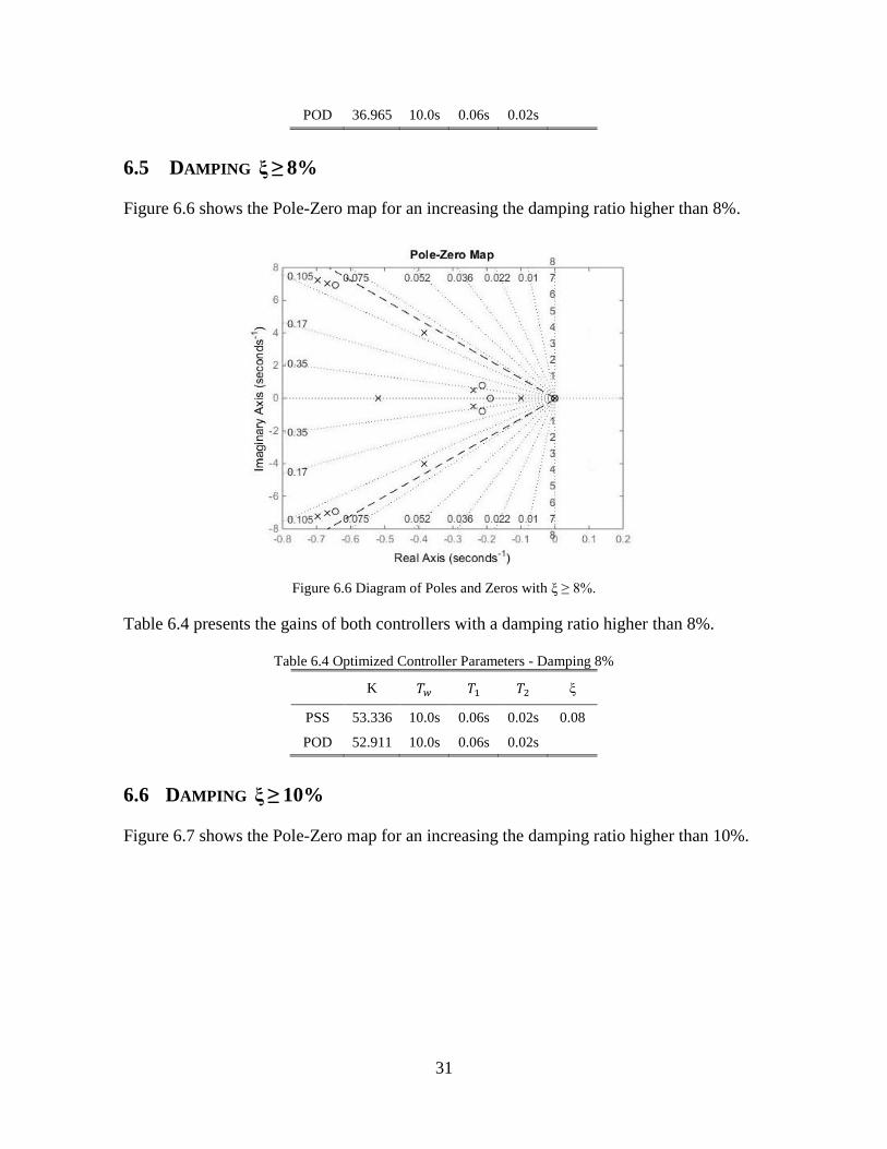
6.5 DAMPING ξ ≥ 8%

Figure 6.6 shows the Pole-Zero map for an increasing the damping ratio higher than 8%.

Figure 6.6 Diagram of Poles and Zeros with ξ ≥ 8%.




PSS 53.336 10.0s 0.06s 0.02s 0.08

POD 52.911 10.0s 0.06s 0.02s

6.6 DAMPING ξ ≥ 10%

Figure 6.7 shows the Pole-Zero map for an increasing the damping ratio higher than 10%.

32

Figure 6.7 Diagram of Poles and Zeros with ξ ≥ 10%.




PSS 71.570 10.0s 0.06s 0.02s 0.10

POD 67.881 10.0s 0.06s 0.02s

Figure 6.5 to 6.7 show the dominant eigenvalues of the test system with PSS and POD

controllers, it is clear that the system with both controllers is stable.

6.7 COMPARISON WITH A DIFFERENT OBJECTIVE FUNCTION

The proposed method is compared with [86]. For a damping of 5%, the gains obtained with

the optimization problem formulated (CDI) at [86] are 𝐾𝑃𝑆𝑆 = 69.9 and 𝐾𝑃𝑂𝐷 = 64.7.

Figure 6.8 to 6.11 show the comparison results. It can see that the controllers computed by

the proposed method preserve the stability under large disturbances. When the fault occurs,

the controllers damp the electromechanical oscillations presented in the system.

33

Figure 6.8 Active Power Flow Through Interconnection of Area 1 to Area 2 – with Supplementary Control.

It is also clear that when the gain of both controllers is increased, the local modes shift

more to the left semi plane, and the damping ratios are more favorable.

Figure 6.9 shows the electrical power oscillations at generator 2 for the different objective

function. As, it is observed, in the first period the oscillation, the power electric decreases

when the fault occurs, but the response of both controllers are fast, after of few second the

electrical power returns to the original value time.

Figure 6.9 Power Generation - Generator 2.

34

Figure 6.10 shows the oscillations in the frequency at generator 2. Once the fault occurs the

machine accelerates, the frequency oscillations are different for both techniques, although

with the proposed method, generator 2 has decelerations softer than CDI, the frequency at

generator 2 stabilizes faster than other generators, because the local controller located in

this machine.

Figure 6.10 Frequency Behavior - Generator 2.

Figure 6.11 shows the SVC voltage bus for the different objective functions. The peak

value of voltage (1.07) has an overshoot (7.1%) is normalized in the second swing, entering

the safe operating limit. The POD controller provides damping overall to the power system

and improves the transient stability.

Figure 6.11 SVC Bus Voltage Behavior.

35

7 ROBUST CONTROLLER COMPUTATION FOR THE TEST

SYSTEM

At the test power system, the central controller sends signals controls to the generator 2

locate in the area 1, also to the SVC FACTS device locate in the middle of the power

system. Figure 7.1 shows the representation of the test system with the robust controller.

Figure 7.1 Test System with the Robust Controller.

The robust controller will be MIMO, multi-input (𝑑𝑤2, 𝑃𝑙) and multi-output (𝑉𝑔𝑒𝑛2, 𝑉𝑆𝑉𝐶),

the selection of the input and output signal is based on modal analysis, it is explained in

Section 3.1.

7.1 MODEL UNCERTAINTIES.

As, it was explained in section 4.2, the uncertainties are computed by comparison of the

frequency responses of several operating conditions versus the base operating condition

taken as base-case for linearization and computation of the control system.

Additionally, taking into account the dynamic order of the system given by (1), that in the

test case is 74; it is applied a Hankel reduction order method [66]-[67] to reduce the

nominal model, such as the dynamic of interest is conserved. The Hankel reduction order

method is a technique based on singular values. So, the full-order of the test system has 74

states, whereas the reduced model is 18 states. These reduced order models are used to

compute the additive uncertainties model.

Figure 7.2 shows the frequency response of different operating conditions. The input

signals that are taken into account are the rotor speed deviation from machine two, and the

36

active power flow through a tie-line that interconnecting areas 1 and 2. In the test case, the

largest uncertainty or difference between the base case and another operating conditions is

when one of the interconnection lines is out of service.

Figure 7.3 shows the largest uncertainty, this is a MIMO system and there will be an

uncertainty for each entry, for issues of simplicity only shows one.

Figure 7.2 Model Uncertainties and Upper Bound.

Figure 7.3 Largest Model Uncertainty.

The upper bound (Figure 7.2) is necessary for the selection of the weighting function 𝑊3

for the robustness in the central controller design. The form of the additive uncertainty is

given by:

37

∆𝑎(𝑠) = [∆𝐺11(𝑠) ∆𝐺12(𝑠)∆𝐺21(𝑠) ∆𝐺22(𝑠)

] (34)

∆𝐺𝑖𝑗(𝑠) =𝑎7𝑠

7 + 𝑎6𝑠6 + ⋯+ 𝑎1𝑠 + 𝑎0

𝑏8𝑠8 + 𝑏7𝑠7 + ⋯+ 𝑏1𝑠 + 𝑏0 (35)

Tables 7.1 and 7.2 show the coefficients of the numerator and denominator of the transfer

functions, that represents the model of additive uncertainty of the test system used to

compute the central controller, these coefficients involve the dynamic of the disturbances in

low frequency.

Table 7.1 Coefficients of the Numerator of ∆𝐺𝑖𝑗(𝑠)

𝑎7 𝑎6 𝑎5 𝑎4 𝑎3 𝑎2 𝑎1 𝑎0

3965 1.08e5 6.18e5 6.53e6 6.33e6 -4.88e7 -1.25e8 20.29

0.98 86.03 360.6 6254 1.65e4 1.19e5 2e5 -0.037

1178 3.17e4 5.03e5 7.25e6 3.49e7 2.35e8 6.75e8 -105.1

1.83 39.62 498.5 220.4 1.47e4 -9.61e4 -4.34e4 -0.013

Table 7.2 Coefficients of the Denominator of ∆𝐺𝑖𝑗(𝑠)

𝑏8 𝑏7 𝑏6 𝑏5 𝑏4 𝑏3 𝑏2 𝑏1 𝑏0

1 25.7 538 3155 2.93e4 8.21e4 2.59e5 5.95e5 -0.093

The coefficients are sorted in the following sequence ∆𝐺11(𝑠), ∆𝐺12(𝑠), ∆𝐺21(𝑠), ∆𝐺22(𝑠),

the denominator is the same for all them.

It is important to know that if exist disturbances bigger than the uncertainties modeled

possibly the robust controller does not work appropriately.

7.2 SELECTION OF WEIGHTING FUNCTIONS.

The weighting functions are both band-pass filter in the frequency range of interest of

electromechanical modes, which is between 0.1 to 3 Hz, the constants 𝑏 corresponding to

the center frequency 𝑓𝑐 of the filter, whereas the constants 𝑐 corresponding to the

attenuation frequency.

The weighting function 𝑊3 is associated with the damping in closed loop, it can play with

the gains of this weighting function to improve the stability of the system, and the damping

ratio depends on the value of these gains 𝐾3. If the objective is to reach a specific damping

ratio, it will have to coordinate these gains to obtain the appropriate value.

The weighting functions are selected as:

38

𝑊1 =

[

𝑠2 + 5

𝑠2 + 2.2𝑠 + 50

0𝑠2 + 5

𝑠2 + 2.2𝑠 + 5]

(36)

𝑊3 = [

2.2𝑠

𝑠2 + 2.2𝑠 + 2.50

02.2𝑠

𝑠2 + 2.2𝑠 + 2.5

] (37)

The output signals affected by the weighting functions are the supplementary voltage

forward signal of the SVC and the AVR of generator 2.

The gains of both weighting functions are taken as 𝐾1𝑑𝑤2= 1, 𝐾1𝑃𝑙 = 1, 𝐾3𝐴𝑉𝑅2

= 1,

𝐾3𝑆𝑉𝐶 = 1, these gains could be tuned once obtained the central controller. Figure 7.4 and

7.5 shows the frequency responses of the inverse of the weighting functions 𝑊1 and 𝑊3.

Figure 7.4 Frequency Response of the Inverse of 𝑊1

39

Figure 7.5 Frequency Response of the Inverse of 𝑊3

7.3 CONTROLLER DESIGN 𝓗∞ MIXED-SENSITIVITY.

The central controller was obtained by running the algorithm explained in section 4.4. The

order of the central controller is 28. To implement the controller in nonlinear simulation,

the order has been reduced in 5 by Hankel model reduction techniques. The transfer

functions of the MIMO controller are:

𝐾11 =−0.87𝑠4 + 3.22𝑠3 − 46.6𝑠2 − 161.7𝑠 + 10.74

𝑠5 + 101.4𝑠4 + 7039𝑠3 + 9261𝑠2 + 3.93𝑥105𝑠 + 3.68 (38)

𝐾12 =3.03𝑠4 − 18.8𝑠3 + 221.5𝑠2 − 908.7𝑠 + 3.2

𝑠5 + 101.4𝑠4 + 7039𝑠3 + 9261𝑠2 + 3.93𝑥105𝑠 + 3.68 (39)

𝐾21 =350.9𝑠4 + 285𝑠3 + 2.76𝑥104𝑠2 − 1.44𝑥104𝑠 + 5.7

𝑠5 + 101.4𝑠4 + 7039𝑠3 + 9261𝑠2 + 3.93𝑥105𝑠 + 3.68 (40)

𝐾22 =−1218𝑠4 + 2620𝑠3 − 6.86𝑥104𝑠2 − 2.67𝑥105𝑠 + 4.08

𝑠5 + 101.4𝑠4 + 7039𝑠3 + 9261𝑠2 + 3.93𝑥105𝑠 + 3.68 (41)

The central controller improves the damping of the power system, the gains were adjusted

at the end empirically, the values are 𝐾1 = 35 and 𝐾3 = 45. Table 7.3 presents the

damping ratios of the closed loop.

40

Table 7.3 Modes of Test System with H∞


-0.284 ± 3.69i 0.59 0.0759

-0.631 ± 6.81i 1.08 0.0923

-0.943 ± 6.63i 1.06 0.1410

The central controller achieved a minimum damping ratio of 7% for the mode more critical

that is inter-area mode. The other local modes also were well damped, now we prove the

behavior of the ℋ∞ controller in the test power system, which it can be seen in the Figure

7.6. The simulated disturbance is the three-phase short circuit in the middle of the line 8-9

that interconnected the areas 1 and 2.

Figure 7.6 Active Power Flow Through the Area 1 to Area 2 After the H∞ Controller.

7.4 CONTROLLER DESIGN 𝓗∞ WITH LMI TECHNIQUES.

The central controller with LMI was obtained by running the algorithm in section 4.5. The

order of the central controller is 28. To perform the new controller, the order has been

reduced in 4 using the same technique of reduction. The transfer functions of these

controllers are:

𝐾11 =0.046𝑠3 − 0.37𝑠2 + 0.036𝑠 − 0.097

𝑠4 + 17.35𝑠3 + 60.97𝑠2 + 7.25𝑠 + 17.78 (42)

𝐾12 =−0.154𝑠3 + 1.41𝑠2 − 0.038𝑠 + 0.431

𝑠4 + 17.35𝑠3 + 60.97𝑠2 + 7.25𝑠 + 17.78 (43)

41

𝐾21 =55.15𝑠3 + 2.885𝑠2 + 22.14𝑠 − 1.182

𝑠4 + 17.35𝑠3 + 60.97𝑠2 + 7.25𝑠 + 17.78 (44)

𝐾22 =−188.8𝑠3 + 39.31𝑠2 − 54.7𝑠 + 17.63

𝑠4 + 17.35𝑠3 + 60.97𝑠2 + 7.25𝑠 + 17.78 (45)

The central controller improves the damping of the power system in the expected value, the

damping ratio selecting is 𝜉 = 10. Table 7.4 presents the damping ratios of the closed loop.

Table 7.4 Modes of Test System with LMI H∞


-0.412 ± 3.81i 0.62 0.104

-0.821 ± 6.85i 1.09 0.118

-0.837 ± 6.61i 1.05 0.125

Table 7.4 demonstrates that the central controller with LMI guarantee the robustness

desired, whereas the standard ℋ∞ controller need to be adjusted with the gains of the

weighting functions. Figure 7.7 shows the behavior of the central controller with LMI.

Figure 7.7 Active Power Flow Through the Area 1 to Area 2 After the H∞ Controller with LMI.

Obviously, the performance of the ℋ∞with the LMI is better than the standard robust

control, since the LMI techniques allow the stronger constraints based on the criterion of

the designer.

42

7.5 CONTROLLER PERFORMANCE EVALUATION WITH DELAYS.

The communication link uses the optic fiber. The time delay range is around 50 to 200 ms

in one single-way include propagation delay. Figure 7.8 shows the representation of test

system with delay signals toward the robust controller.

Figure 7.8 Test System with Delay Signals.

Figure 7.9 shows the performance of both robust central controllers computed previously

for the test system, when the system is perturbed by a three-phase short circuit in the

middle of interconnection line 8-9 between area 1 and 2.

In spite of applying time delays of way random in different timeslots the performance of

the both robust controllers is well. It is important to say that the response of both robust

controller are better with time delays because the robust controllers are not acting when the

disturbance occurs, the robust controllers start their control action 100 ms after the control

signals arrive.

43

Figure 7.9 Active Power Flow Through the Area 1 to Area 2 with Delay Signals.

7.6 COMPARISON OF DIFFERENT TECHNIQUES 𝓗∞.

The designed of both controllers is evaluated, nonlinear simulations have been carried out

for the largest disturbance in a time period of 20s. The results are compared between the

standard and LMI ℋ∞ techniques. Figure 7.10 to 7.12 show the responses for different state

variables. The simulated disturbance is the three-phase short circuit in the middle of the line

8-9 that interconnected the areas, exporting 413 MW from area 1 to area 2.

Figure 7.10 Power Generation – Generator 2.

44

Figure 7.11 Frequency Response – Generator 2.

Figure 7.12 SVC Bus Voltage Behavior.

The simulation results have pointed out that both robust controllers can maintain the

stability under different operating conditions. The LMI ℋ∞ technique can provide greater

damping than the standard. The transient stability is improved by the effect of SVC in the

tie-line.

45

8 CONCLUSION

This thesis presents a methodology for the coordinated tuning of the PSS and POD

controller based on an algorithm optimization. The methodology is based on the linearized

power system model and parameter constrained nonlinear optimization technique. Using a

model reduced by the system to simplify the calculation.

The reduced model can be used to facilitate the design of damping controllers, it has been

demonstrated with a reduced model of approximately 1/5𝑡ℎ of the size of the original

model.

The results obtained from the test system using the coordinated tuning method revealed that

adequate damping could be achieved by increasing the gains of both controllers.

Although the SVC is simulated in the proposed test system, the algorithm is in general

applicable to others kind of FACTS device.

On the other hand, the methodology for the computation of robust controllers to reduce the

impact of low frequency oscillations is developed, applying ℋ∞ mixed sensitivity

technique (standard and LMI), that guarantee robustness in a wide range of operating

conditions of a power system; such as contingencies, uncertainties and delays in the signals.

The thesis proposes a detailed modeling of uncertainties of the power system as additive

uncertainties of the plant under the theory of robust control, based on the frequency

response comparison of several operating conditions of the power system.

Also, the thesis presents a methodology for defining the appropriate computation of the best

weighting functions based on these uncertainties and control purposes (damping of

electromechanical oscillations). It is also proposed the computation of robust controllers in

two stages guaranteeing robustness and damping, and the analysis of performance of the

controller against delays in control signals

The reduction order modelling of the power system and also of the controller has been

carried out showing good performance.

The following statement must be considered to build a robust controller for the damping of

electromechanical oscillations in the power system:

The model uncertainties either additive or multiplicative must be modeled in the

range of frequency of interest.

The magnitude in all ranges of frequency of the weighting functions should be

larger than the uncertainties.

With proper formulation, the ℋ∞ technique can provide a suitable damping to the power

system. The LMI technique has more complexity, but it has compensated with flexibility of

obtaining a desired damping ratio overall of the power system.

46

Time delays in the input signal torward the robust controller does not affect the control

action in overall power system.

47

REFERENCES

[1]. P. Kundur, Power System Stability and Control, New York: McGraw-Hill, Inc., 1994, pp. 3-168, 699-

825, and 1103-1166.

[2]. G. Rogers, Power System Oscillations, New York: Kluwer Academic Publishers, 2000, pp. 1-6, 7-30,

31-73, and 139-168.

[3]. L. Angquist, B. Ludin, and J. Samuelsson, “Power oscillation damping using controlled reactive power

compensation-a comparison between series and shun approaches,” IEEE Transactions on Power

Systems, vol. 8, no. 2, pp. 687-700, May 1993.

[4]. I. Kamwa, “Performance of three PSS for inter-area oscillations,” SymPowerSystems Toolbox.

[Online]. Available at: http://www.mathworks.com/help/physmod/sps/examples/performance-of-three-

pss-for-interarea-oscillations.html.

[5]. E. V. Larsen, and D. A. Swann, “Applying power system stabilizers part I: General concepts,” IEEE

transactions on Power Apparatus and Systems, vol. PAS-100, no. 6, pp. 3017-3024, June 1981.

[6]. Western Electricity Coordinating Council, “WECC-0107 VAR-501-WECC-2 power system stabilizer

posting 1, 28 May 2014 [Online]. Available at: https://www.wecc.biz/Standards/Pages/WECC-

0107.aspx.

[7]. R. G. Farmer, “Independent detection scheme to initiate western system islanding for pacific AC

intertie outages,” Paper presented at the panel session on controlled separation and load shedding,

IEEE PES summer meeting, 1985.

[8]. .A. Sharma, and M. L. Kothari, “Intelligent dual input power system stabilizers for multi-machine

system,” Transmission and Distribution Conference and Exhibition 2002: Asia Pacific. IEEE/PES,

Jodhpur, 2002.

[9]. Asea Brown Boveri, “UNITROL stand-alone power system stabilizer,” 2005 [Online]. Available at:

https://library.e.abb.com/public/884b34036f7fba22c125774a0047e9da/3BHT490395_E01_A_O.pdf

[10]. Mitsubishi Electric Corporation, “Power system stabilizer,” Septermber 2010 [Online]. Available at:

http://www.meppi.com/Products/GeneratorExcitationProducts/Pages/default.aspx.

[11]. General Electric Corporation, “Power system stabilizer,” 2015 [Online]. Available at:

http://alstomenergy.gepower.com/products-services/product-catalogue/power-generation/coal-and-oil-

power/automation-and-controls-for-coal-and-oil/power-system-stabilizer/.

[12]. J. H. Chow, G. E. Boukarim, and A. Murdoch, “Power system stabilizers as undergraduate control

design projects,” IEEE Transactions on Power Systems, vol. 19, no. 1, February 2004.

[13]. W. Watson, and G. Manchur, “Experience with supplementary damping signals for generator static

excitation systems,” IEEE Transactions on Power Apparatus and Systems, vol. PAS-92, no. 1, pp. 199-

203, January 1973.

[14]. K- E. Bollinger, W. Gu. , and E. Norum, “Accelerating power versus electrical power as input

signals to power system stabilizers,” IEEE Transactions on Energy Conversion, vol. 6, no. 4, pp. 620-

626, December 1991.

[15]. V. M. Raina, J. H. Anderson, W. J. Wilson, and V. H. Quintana, “ Optimal output feedback control

of power ystems with high-speed excitation systems,” IEEE Transactions on Power Apparatus and

Systems, vol. PAS-95, no. 2, March 1976.

48

[16]. C. Wu, and Y. Hsu, “Design of self-tuing PID power system stabilizer for multimachine power

systems,” IEEE Transactions on Power Systems, vol. 3, no. 3, pp. 1059-1064, August 1988.

[17]. M. K. El-Sherbiny, M. M. Hasan, G. El-Saady, and A. M. Yousef, “Optimal pole shifting for power

system stabilization,” Electric Power Systems Research, vol. 66, no. 3, pp. 253-258, September 2003.

[18]. H. Othman, J. J. Sanchez-Gasca, M. A. Kale, and J. H. Chow, “On the design of robust power system

stabilizers,” The 28th Conference on Decision and Control, Tampa, 1989.

[19]. Y. Yu., and Q. Li, “Pole-placement power system stabilizers design of an unstable nine-machine

system,” IEEE Transactions on Power Systems, vol. 5, no. 2, pp. 353-358, May 1990.

[20]. G. Radman, “Design of power system stabilizer based on LQG/LTR formulations,” Conference

Record of the 1992 IEEE Industry Applications Society Annual Meeting, Houston, 1992.

[21]. M. Nambu, and Y. Ohsawa, “Development of an advanced power system stabilizer using a strict

linearization approach,” IEEE Transactions on Power Systems, vol. 11, no. 2, pp. 813-818, May 1996.

[22]. A. K. Sedigh, and G. Alizadeh, “Design of robust power system stabilizers (PSS) using quantitative

feedback theory,” International Conference on Control, Coventry, 1994.

[23]. A. F. Okou, M. Kelemen, L. A. Dessaint, and O. Akhrif, “Towards a systematic procedure to design

robust power system stabilizers,” IEEE Power Engineering Society Summer Meeting, Seatle, 2000.

[24]. S. S. Sharif, “Nonlinear power system stabilizer design technique,” Canadian Conference on

Electrical and Computer Engineering¸ Montreal, 1995.

[25]. F. E. Scavoni, A. S. e Silva, A. T. Neto, and J. M. Campagnolo, “Desing of robust power system

controllers using linear matrix inqualities,” IEEE Porto Power Tech Conference, Porto, 2001.

[26]. A. Soós, and O. P. Malik, “An 𝐻2 optimal adaptive power system stabilizer,” IEEE Transactions on

Energy Conversion, vol. 17, no. 1, pp. 143-149, March 2002.

[27]. A. Sil, T. K. Gangopadhyay, S. Paul, and A. K. Maitra, “Design of robust power system stabilizer

using H∞ mixed sensitivity technique,” The 3th International Conference on Power Systems,

Kharagpur, 2009.

[28]. Y. Hsu, and C. Chen, “Tuning of power system stabilizers using an artificial neural network,” IEEE

Transactions on Energy Conversion¸vol. 6, no. 4, pp. 612-619, December 1991.

[29]. Y. M. Park, and K. Y. Lee, “A wide range operation power system stabilizer design with neural

networks using power flow characteristics,” International Conference on Intelligent Systems

Applications to Power Systems, Orlando, 1996.

[30]. P. Shamsollahi, and O. P. Malik, “Design of a neural adaptive power system stabilizer using dynamic

back-propagation method,” International Journal of Electrical Power & Energy Systems, vol. xx, no. x,

January 2000.

[31]. A. Ishigame, T. Ueda, S. Kawamoto, T. Taniguchi, and M. Kikuta, “Desing of electric power system

stabilizer based on fuzzy control theory,” IEEE International Conference on Fuzzy Systems, San Diego,

1992.

[32]. J. Shi, L. H. Herron, A. Kalam, “Comparison of fuzzy logic based and rule based power system

stabilizer,” The 1th IEEE Conference on Control Applications, Dayton, 1992.

[33]. G. V. Moodley, G. D. Jennings, R. G. Harley, and M. T. Wishart, “Fuzzy logic power system

stabilizer in multimachine stability studies,” 1996 IEEE AFRICON 4th AFRICON conference in Africa,

Stellenbosch, 1996.

49

[34]. A. Ghosh, G. Ledwich, O. P. Malik, and G. S. Hope, “Power system stabilizer based on adptive

control technique,” IEEE Transactions on Power Apparatus and Systems, vol. PAS-103, no. 8, pp.

1983-1989, August 1984.

[35]. W. Gu, “Sysmtem damping improvement using adaptive power system stabilizer,” The 1999 IEEE

Canadian Conference on Electrical and Computer Engineering, Edmonton, 1999.

[36]. W. Liu, G. K. Venayagamoorthy, and D. C. Wunsch, “A heuristic-dynamic-programming-based

power system stabilizer for a turbogenerator in a single-machine power system,” IEEE Transactions on

Industry Applications, vol. 41. No. 5, September/October 2005.

[37]. C. Lu, Y. Zhao, K. Men, L. Tu, and Y. Han, “Wide-area power system stabilizer based on model-free

adaptive control,” The Institution of Engineering and Technology (IET) Control Theory & Applications,

vol. 9, no. 13, pp. 1996-2007, August 2015.

[38]. A. H. Ahmad, and A. A. Abdelqader, “Power system stabilizer design using real-coded genetic

algorithm,” The 2th International Conference on Control, Instrumentation and Automation, Shiraz,

2011.

[39]. M. A. Abido, “Robust design of multimachine power system stabilizers using simulated annealing,”

IEEE Transactions on Energy Conversion, vol. 15, no. 3, pp. 297-304, September 2000.

[40]. M. A. Abido, “Optimal design of power system stabilizers using particle swarm optimization,” IEEE

Transactions on Energy Conversion, vol. 17, no. 3, pp. 406-413, September 2002.

[41]. I. Kamwa, L. Gerin-Lajoie, and G. Trudel, “Multi-loop power system stabilizers using wide-area

synchronous phasor measurements,” The American Control Conference, Philadelphia, 1998.

[42]. N. N. Islam, M. A. Hannan, H. Shareef, and A. Mohamed, “Power system stabilizer design using

BAT optimization algorithm in multimachine power system,” IEEE Student Conference on Research

and Development, Putrajaya, 2013.

[43]. S. Zhang, and F. L. Luo, “An improved simple adaptive control applied to power system stabilizer,”

IEEE Transactions on Power Electronics, vol. 24, no. 2, pp. 369-375, February 2009.

[44]. V. K. Chandrakar, S. N. Dhurvey, and S. C. Suke, “Performance comparison of SVC with POD and

PSS for damping of power system oscillations,” The 3th International Conference on Emerging

Trendes in Engineering and Technology¸ Goa, 2010.

[45]. D. Cerón, and M. A. Ríos, “Decentralized control for FACTS (SVC and TCSC) using POD in power

systems,” IEEE ANDESCON, Bogota, 2010.

[46]. S. P. Teeuwsen, “STATCOM with optimized POD controller for efficient inter-area oscillation

damping,” 2013 IEEE Power & Energy Society General Meeting, Vancouver, 2013.

[47]. L. J. Cai, and I. Erlich, “Fuzzy coordination of FACTS controllers for damping power system

oscillations,” International Symposium on Modern Electric Power System. Wroclaw, 2002.

[48]. K. C. Rout, and P. C. Panda, “Performance analysis of power system dynamic stability using fuzzy

logic based PSS for positive and negative value of K5 constant,” International Conference on

Computer, Communication and Electrical Technology, Tamilnadu, 2011.

[49]. X. Lei, E. N. Lerc, and D. Povh, “Optimization and coordination of damping controls for improving

systems dynamic performance,” IEEE Transactions Power Systems, vol. 16, no. 3, pp. 473-480, August

2001.

50

[50]. J. J. Sanchez Gasca, and J. H. Chow, “Power system reduction to simplify the design of damping

controllers for inter-area oscillations,” IEEE Transactions on Power Systems, vol. 11, no. 3, pp. 1342-

1349, August 1996.

[51]. P. Pourbeik, and M. J. Gibbard, “Simultaneous coordination of power system stabilizers and FACTS

device stabilizers in a multimachine power system for enhancing dynamic performance,” IEEE

Transactions on Power Systems, vol. 13, no. 2, pp. 476-479, May 1998.

[52]. D. Arnautovic, and J. Medanic, “Design of decentralized multi-variable excitation controller in

multi-machine power systems by projective controls,” IEEE Transactions on Energy Conversion, vol.

EC-2, no. 4, pp. 598-604, December 1987.

[53]. K. Zhou, J. C. Doyle, K. Glover, Robust and Optimal Control, New Jersey: Prentice-Hall, Inc, 1996,

pp. 213-245, and 413-446.

[54]. B. Pal, B. Chaudhuri, Robust Control in Power Systems, New York: Springer, 2005, pp. 13-36, 59-

75, and 115-136.

[55]. S. Skoegestad, I. Postlethwaite, Multivariable Feedback Control Analysis and Design, Chichester:

John Wiley & Sons, Ltd, 2005, pp. 259-288, 341-381, and 473-490.

[56]. H. Jia, N. Guangyu, S. T. Lee, and P. Zhang, “Study on the impct of time delay to powe system small

signal stability,” 2006 IEEE Mediterranean Electrotechnical Conference, Malaga, 2006.

[57]. F. Milano, and M. Anghel, “Impact of time delays on power system stability,” IEEE Transactions on

Circuits and Systems I, vol. 59, no. 4, April 2012, pp. 889-900.

[58]. B. Chaudhuri, R. Majumder, and B. Pal, “Wide area measurement based stabilizing control of power

system considering signal transmission delay,” IEEE Transactions on Power Systems, vol. 19, no. 4,

November 2004, pp. 1971-1979.

[59]. J. Chen, G. Gu, and C. N. Nett, “A new method for computing delay margins for stability of linear

delay systems,” System and Control Letters, vol .26, no. 2, September 1995, pp. 107-117.

[60]. B. Naduvathuparambil, M. Valenti, and A. Feliachi, “Communication delays in wide-area

measurement systems,” Proceedings of the 34th Southeastern Symposium on System Theory,

Morgantown, 2002.

[61]. E. V. Larsen, and D. A. Swann, “Applying power system stabilizers part II: performance objectives

and tuning concepts,” in IEEE Transactions on Power Apparatus and Systems, vol. PAS-100, no. 6, pp.

3025-3033, June 1981.

[62]. K. R. Padiyar, Power System Dynamics Stability and Control. Chichester: Jhon Wiley & Son, Ltd,

Singapore, 1996, pp. 257-291.

[63]. R. Narne, P. C. Panda, and J. P. Therattil, “Genetic algorithm based simultaneous coordination of

PSS and FACTS controllers for power oscillations damping,” 2012 IEEE the 3th International

Conference on Sustainable Energy Technologies, Kathmandu, 2012.

[64]. M. A. Abido, “Design of PSS and STATCOM-based damping stabilizers using genetic algorithms,”

2006 IEEE Power Engineering Society General Meeting, Montreal, 2006.

[65]. M. Hajizadeh, and J. Sadeh, “Simultaneous coordination and tuning of PSS and FACTS for

improving damping by genetic algorithm,” 2011 4th International Conference on Electric Utility

Deregulation and Restructuring and Power Technologies, Weihai, 2011.

[66]. M. G. Safonov, and R. Y. Chiang, “A Schur method for balanced-truncation model reduction,” IEEE

Transactions on Automatic Control, vol. 34, no. 7, pp. 729-733, July 1989.

51

[67]. B. Moore, “Principal component analysis in linear systems: controllability, observability, and model

reduction,” IEEE Transactions on Automatic Control, vol. AC-26, no. 1, pp. 17-31, February 1981.

[68]. A. J. Laub, M. T. Heath, C. C. Paige, and R. C. Ward, “Computation of system balancing

transformations and their applications of simultaneous diagonalization algorithms,” IEEE Transactions

on Automatic control, vol. AC-32, no. 2, pp. 115-122, February 1987.

[69]. J. H. Chow, L. P. Harris, M. A. Kale, H. A. Othman, J. J. Sanchez Gasca, and G. E. Terwilliger,

“Robust control design of power system stabilizers using multivariable frequency domain techniques,”

The 29th IEEE Conference on Decision and Control, Honolulu, 1990.

[70]. A. Sil, T. K. Gangopadhyay, S. Paul, and A. K. Maitra, “Design of robust power system stabilizer

using H∞ mixed sensitivity technique,” The 3th International Conference on Power Systems,

Kharagpur, 2009.

[71]. Q. Zhao, and J. Jiang, “Robust SVC controller design for improving power system damping,” IEEE

Transactions on Power Systems, vol. 10, n. 4, November 1995, pp. 1927-1932.

[72]. R. W. Beaven, M. T. Wright, and D. R. Seaward, “Weighting function selection in the H∞ design

process,” Control Engineering Practice, vol. 4, n. 5, May 1996, pp. 625-633.

[73]. K. Monwane, and K. A. Folly, “Robustness evaluation of H∞ power system stabilizer,” IEEE Power

& Energy Society (PES) Power Africa 2007, Conference and Exhibition Johannesburg, Johannesburg,

2007.

[74]. B. Chaudhuri, B. C. Pal, A. C. Zolotas, I. M. Jaimoukha, and T. C. Green, “Mixed sensitivity

approach to H∞ control of power system oscillations employing multiple FACTS devices,” IEEE

Transactions on Power Systems, vol. 18, n. 3, August 2003, pp. 1149-1156.

[75]. M. Bouhamida, A. Mokhatri, and M. A. Denai, “Power system stabilizer design based on robust

control techniques,” American Society of Civil Enginerrs (ACSE) Journal, vol. 5, n. 3, November 2005,

pp. 33-41.

[76]. Y. Peng, Q. M. Zhu, H. Nouri, Robust H2 power system stabilizer design using LMI techniques,

2011 International Conference on Modelling, Identification and Control, June 26-29, 2011, Shanghai,

China.

[77]. P. Gahinet, P. Apkarian, A linear matrix inequality approach to H∞-control, International Journal

Robust and Nonlinear Control, vol. 4, n. 4, 1994, pp. 421-448.

[78]. T. Iwasaki, R. E. Skelton, All controllers for the general H∞-control problem: LMI existence

conditions and state space formulas, Automatica, vol. 30, n. 8, 1994, pp. 1307-1317.

[79]. A. N. Cuk Supriyadi et al., Inverse additive perturbation-based optimization of robust PSS in an

interconnected power system with wind farms, Society of Instrument and Control Engineers (SICE)

Annual Conference 2008, Tokyo, 2008.

[80]. H. Bevrani, Robust power system frequency control. New York: Springer, 2009, pp. 71-103, and

105-129.

[81]. C. Zhu, M. Khammash, V. Vittal, and W. Qiu, “Robust power system stabilizer design using H∞

loop shaping approach,” IEEE Transactions on Power Systems, vol. 18, n. 2, May 2003, pp. 810-818.

[82]. K. Glover, J. C. Doyle, “State-space formulae for all stabilizing controllers that satisfy an H∞ norm

bound and relations to risk sensitivity,” Systems & Control Letters, vol. 11, n. 8, 1988, pp. 167-172.

52

[83]. J. C. Doyle, K. Glover, P. Khargonekar, and B. Francis, “State-space solutions to standard H2 and

H∞ control problems,” IEEE Transactions on Automatic Control, vol. 34, n. 8, August 1989, pp. 831-

847.

[84]. M. G. Safonov, D. J. N. Limebeer, and R. Y. Chiang, “Simplifying the H∞ theory via loop shifting,

matrix pencil and descriptor concepts,” International Journal Control, vol. 50, n. 6, 1989, pp. 2467-

2488.

[85]. M. Eslami, H. Shareef, and A. Mohamed, “Coordinated design of PSS and TCSC controller for

power system stability improvement,” 2010 Conference International Symposium on Parameterized

and Exact Computation, Singapore, 2010, pp 433-438.

[86]. Cai L.J, and I. Erlich, “Simultaneous coordinated tuning of PSS and FACTS damping controllers in

large power systems,” IEEE Transactions on Power Systems, vol. 20, no. 1 February 2005, pp. 294-

300.

Documents

STRATEGIES OF COORDINATED CONTROL OF PSS AND POD IN …