Embed Size (px)
Citation preview

IFN Working Paper No. 1015, 2014 Strategic Withholding through Production Failures Sara Fogelberg and Ewa Lazarczyk
Research Institute of Industrial Economics P.O. Box 55665
SE-102 15 Stockholm, Sweden [email protected] www.ifn.se
1
Strategic withholding through production failures1
by Sara Fogelberg2 and Ewa Lazarczyk3
February 20, 2014
Abstract
Anecdotal evidence indicates that electricity producers use production failures to disguise
strategic reductions of capacity in order to influence prices, but systematic evidence is lacking.
We use a quasi-experimental set up and data from the Swedish energy market to examine such
behavior. In a market without strategic withholding, the decision of reporting a failure should be
independent of the market price. We show that marginal producers in fact base their decision to
report a failure in part on prices, which indicates that failures are a result of economic incentives
as well as of technical problems.
JEL: L49, L94.
Key words: Electricity markets, Urgent Market Messages (UMMs), unplanned failures,
withholding, economic incentives, IV.
1 We are grateful for comments from Richard Friberg, Mårten Palme, Mikael Priks, Thomas Tangerås, Pär Holmberg, Sven-‐Olof Fridolfsson, John Kwoka, Estelle Cantillon, Erik Lindqvist, Yoichi Sugita and Johanna Rickne as well as seminar participants at Stockholm School of Economics and Research Institute of Industrial Economics (IFN), conference participants at YEEES 2013 in Stockholm and seminar participants at ECARES. The work has been financially supported by the Research Program” The Economics of Electricity Markets”. 2 Stockholm University and IFN, Universitetsvägen 10 A, 106 91 Stockholm, Sweden, +46 8 16 42 42, E-‐mail: [email protected]
3 Research Institute of Industrial Economics (IFN), P.O. Box 55665, SE-‐102 15 Stockholm, Sweden, fax + 46 8 665 4599,E-‐mail
[email protected]; Stockholm School of Economics, Department of Economics, Sveavägen 65, Stockholm, Sweden. E-‐mail [email protected]
2
- We decided the prices were too low... so we shut down. - Excellent. Excellent. - We pulled about 2,000 megs of the market. -That's sweet. - Everybody thought it was really exciting that we were gonna play some market power. That was fun! Intercepted exchange between Reliant traders, June 2000, Weaver (2004).
1. Introduction
Competitive and well-functioning market is one of the goals of modern, liberalized electricity
markets. However, a commonly voiced concern has been that firms strategically reduce their
generating capacity in order to increase the electricity price. Strategic withholding of electricity
was for example observed during the electricity crisis in 2000-2001 in California and has been
determined to be one of the reasons why the crisis became so severe (Kwoka and Sabodash 2011
and Weaver 2004). Theoretical studies have also shown how firms benefit from this behavior
(Crampes and Creti 2005, Kwoka and Sabodash 2011). On the other hand, Scandinavia studies
of market power investigating the Nordic electricity market Nord Pool have so far been
inconclusive (Vassilopoulous 2003, Hjalmarsson 2000 and Fridolfsson and Tangeras 2009).
In this paper we look at a previously unexamined way through which electricity producers can
withhold capacity to increase prices on the Nordic electricity market. We consider instances
when generators shut down part of their production due to a failure and we verify whether the
decision to stop production and inform about this failure depends on economic incentives as
opposed to being a result of a technical problem. Market participants on Nord Pool are obliged
3
to publicly inform about changes to consumption, generation or transmission that exceed
100MW and that last longer than 60 minutes in so called Urgent Market Messages (UMMs). We
investigate whether spot prices on Nord Pool influence the probability of production failures
reported in UMMs. A decision about reporting a failure should be independent of prices as
failures should be irregular and difficult to foresee. Detection of a significant relationship
between prices and market messages therefore indicates that market participants base decisions
concerning reporting a failure not only on technical problems but also on economic incentives.
We use a unique dataset containing UMMs released by market participants with information
about planned and unplanned reductions of production. Our dataset permits us to examine how
prices affect market participants’ decision about issuing failure messages and how this decision
varies by the type of generator. We distinguish messages issued by different types of baseload
unit production, i.e., nuclear and hydro4, and marginal unit production, i.e., coal, gas and oil.
When the demand is high a small reduction in produced quantity can have a large impact on
prices and this reduction can be achieved both by a marginal or a baseload unit. However, a
producer with several types of generators primarily has an incentive to decrease production for
marginal fuel types since these production units have higher marginal costs. We hence expect
larger effects for marginal fuel types which in the case of Sweden is oil, gas and coal.
We also separate the effects for new messages regarding failures and follow-up messages
concerning already reported failures. This distinction is important as the incentives might differ
depending on whether a generator decides on the new failure or on the prolongation of an
4 Although hydro generation, especially with reservoirs, can be thought of as marginal type of generation due to its fast response
time and balancing characteristics, in this analysis we treat hydro as baseload. We make a distinction between types of electricity
generation with regard to the level of marginal costs as low costs generators will face different incentives than high cost
generators.
4
existing outage. It is possible that a generator decides to report a new failure based on the
encountered technical problems, but that the decision on the length of the failure depends on
economic incentives. An increased number of follow up messages indicates that it takes longer
time to fix a failure, and the time it takes to fix a failure should not depend on prices in a
competitive market.
We use a linear two step model where we estimate the effect of prices on the number of UMMs
being released on a certain day. Because of endogeneity problems between prices and failures
reported in UMMs, we instrument for prices using daily temperatures. For instance, prices could
affect how generators are operated, which could also affect failure rates. Temperature was
chosen as an instrument due to its exogenous nature and since prices on the Nordic electricity
market are highly correlated with temperature. Especially during the cold season, when
electricity is used for heating, temperature and demand follow each other closely.
To our knowledge, this is the first paper studying strategic withholding that uses a quasi-
experimental set up. The results indicate that there is a significant relationship between day-
ahead electricity prices and the number of reported failures. The size of the effect depends on the
type of fuel used for generation. We find positive effects of an increase of price on the number of
reported failures in case of marginal technologies, that is oil and gas. Prices have a larger effect
on follow-up messages compared to messages reporting an initial failure.
We first describe the economic rationale for withholding capacity in Section 2, followed by a
description of the Nordic electricity market in Section 3. The data used in the analysis is
presented in section 4. Section 5 presents the econometric strategy and results are discussed in
Section 6. The last section concludes.

5
2. Economic rationale for withholding capacity
Strategic withholding is regarded as a way of exploiting market power on electricity markets. A
multi-unit generator that wants to increase the market price can achieve it in two ways. It can
either bid strategically all of its production asking for high prices (above its marginal costs5), or
it can physically keep some of its capacity away from the market6. This paper deals with a
specific version of physical withholding, reduction of capacity through production failure. In the
literature we refer to, and in this paper, “strategic” is not defined as an interaction between
multiple market players, but as a unilateral decision of one player to systematically influence
prices (Wolfram 1998, Kwoka and Sabodash 2011). Another important distinction is that even
though strategic withholding is considered as uncompetitive behavior, a form of market power
abuse, an individual firm engaging in this behavior does not need to possess large market share
for withholding to be advantageous (Kwoka and Sabodash 2011, Kwoka 2012). In order for the
strategic withholding to be profitable, a producer needs to own several production units and the
increase in profit after a production failure needs to be larger than the lost profit from the
withheld generation.
We illustrate physical withholding behavior and its attempted impact on the prices in Figure 1.
The graph depicts characteristics of a liberalized wholesale electric power market with inelastic 5 This form of capacity withholding is often referred to as “economic withholding” Moss (2006). 6 For the first alternative see for e.g. Wolfram (1998) where it is shown that in England large suppliers bid strategically above
their marginal costs and that all power plants submit higher bids if their owner has more low-cost capacity available. Wolfram
(1999) has as well evaluated prices in the spot market, comparing several price-cost ratios with the outcomes of theoretical
oligopoly models and concluded that capacity withholding did not result in as high markups as the theory would suggest.

6
demand (in the short run) and a hockey-stick supply curve. The special shape of the supply curve
is due to the merit order of electricity production, that is, the ordering of electricity production
technologies according to their increasing marginal cost of production. Electricity is supplied by
either baseload production with large starting costs but low, almost zero, marginal cost (for
instance nuclear power plants), or by marginal production that starts producing when the
baseload cannot fulfill the demand (for instance coal or gas in the Nordic energy market).
Moreover, different plants have some fixed capacity with steady cost which rises sharply when
this capacity is exceeded.
Figure 1. Wholesale electricity market, capacity withholding.
The Scandinavian electricity market operates as a uniform auction resulting in a single
equilibrium price for each hour. A reduction of supplied quantity shifts the supply curve to the
left which can result in big price changes, especially if the demand curve is close to the almost

7
vertical part of supply curve. This is the explanation to why even producers with a small share
of the market can gain from strategic withholding if demand is high.
We expect different production technologies to have different incentives for strategic
withholding and we anticipate finding larger effects for marginal production technologies.
Withholding marginal production is more profitable since these units have higher marginal costs
compared to baseload units. When demand is high and marginal production units set the price,
even a small reduction of capacity can have a substantial impact on prices. Under these
circumstances the market price is higher than the marginal cost of baseload production so it is in
the interest of cheap, baseload generation to produce. For technical reasons it is as well easier to
shut down a marginal production unit compared to a baseload production unit. In the Nordic
electricity market nuclear and hydro are considered baseload technologies and oil, gas and coal
are considered marginal technologies. Hence, we expect larger effects for coal, gas and oil.
2.1 Strategic withholding through failures
In contrast to the withholding literature that focuses on bidding strategies of operators, we
analyze the strategy of physical withholding of capacity. We assume that producers have an
incentive for disguising withholding as failures. This strategy, as opposed to simply increasing
bid prices, has an advantage of being more difficult to prove simply by looking and comparing
bid curves of market participants and can always be explained as undertaken due to technical
reasons or due to security issues. We assume that disguising capacity withholding as failures can
give firms an option of claiming to be doing their best in providing generating services under the
8
circumstances. Physical withholding has been examined in the literature concerning price spikes7
but as Kwoka (2012) points out, the occurrence of extreme price spikes have gone down in most
deregulated markets the last few years. It is possible that the attention media and research has
brought to the subject has made markets participants more careful. There is however still scope
for strategic withholding through production failures given that this strategy is difficult to prove
and has not been systematically investigated until in this paper.
It is possible that there is no systematic timing of failures, but that the time it takes to correct a
failure depends on economic incentives. There has been anecdotal evidence of similar behavior
played at the British electricity pool, where generators have occasionally prolonged the outage if
doing so they could receive higher level of capacity payments (Newbery, 1995; Green, 2004). In
this paper we separate the effects for failures reported for the first time and for follow-up
messages regarding already reported failures. More follow-up messages indicate that it takes
longer time to fix a failure. If the effects that we estimate are larger for follow-up messages
compared to reports of new failures we can conclude that firms put more emphasis on prolonging
failures compared to timing them strategically and announcing them for the first time.
2.2 Spot prices and timing
By the design of the Nordic electricity market, the next day’s electricity prices are set on the
previous day at 1 p.m. Prices are correlated over time and in case there are no shocks the
expected price for tomorrow’s electricity is equal to today’s price. Therefore we assume that a 7 Kwoka and Sabodash (2011) develop a method to separate price spikes that are a result from demand shifts under inelastic supply from price spikes that result from strategic withholding. They do this by investigating whether supply systematically shifts down during periods of high demand. They conclude that there is evidence of strategic withholding for a brief period of time during 2001 on the New York wholesale electricity market. They also develop a model that shows that unilateral withholding for a company with two identical production units is profitable, as long as the price increase (resulting from reduction of capacity) is larger than the initial price-cost margin.
9
producer would base the decision of reporting a failure on today’s price. A failure cannot
influence the current spot price as this is already fixed. It can however have an impact on the
next day’s price. Today’s production failure will become common knowledge through UMMs.
Tomorrow’s prices will increase if other producers fail to compensate for this failure. Another
scenario assumes that when a failure happens a more expensive unit produces the missing
capacity which is likely to happen when demand is binding. All this will result in today’s failure
pushing up tomorrow’s prices8.
In our framework we focus only on the day-ahead market, the spot price, excluding from our
analysis possible interactions between markets of different horizons, for instance balancing and
future markets. Given our econometric set up we can only estimate how daily variations in price
affect failure rates which mean that any long term withholding strategies are outside the scope of
this paper.
2.3 A simple example
In this section we illustrate with simplified calculations how withdrawing of capacity from the
market can be a profitable strategy. We use price numbers from our data that we will more
carefully go through in the data description part of this paper. We assume that marginal
production costs are zero for all types of units.
Consider a producer A, who owns 1000MW production that can be divided into 10 units of 100
MW each. In the warm season, from the 15th of March until the 1st of October, the mean price
in our sample is 36€. In order not to lose on withdrawing 100MW of capacity the price increase 8 We estimate the impact of failures on the next day’s spot price in tables 10 and 11 (see in the Appendix).
10
as a result to this capacity reduction would need to be at least 4€. If the producer decides not to
fail he can earn 36000 € [1000MW*36€], if he however decides to fail 100MW, the price would
have to be 40€ in order for the producer to enjoy the same profit [900MW*40€=36000€].The
situation is almost the same in the cold period (1st of October – 15th of March) when the mean
price is 44€. In this season the price would need to increase by 4,8€ for the producer to be
indifferent on whether to reduce capacity by 100MW or not [44€*1000MW=44000€ vs.
49€*900MW=44100€].
In the analyzed time period the mean of the difference between today’s price and yesterday’s
price is almost zero and the standard deviation is 5.51€. This indicates that the minimal price
change from day to day, necessary for producer A to not loose on withdrawing capacity (4-5€) is
realistic. Moreover, the maximal day to day average price difference observed for the analyzed
time frame is 33€.
3. Market description
The Scandinavian electricity market is one of the first deregulated electricity markets in the
world and the largest European electricity market both in turnover and geographical area. It
consists of seven countries belonging to the Nordic and Baltic region i.e. Sweden, Norway,
Finland, Denmark, Lithuania, Estonia and Latvia9. The market is also connected with other
countries e.g. Germany, Poland and UK. It consists of physical and financial markets. Two
physical markets form the Nord Pool Spot and enable trading with the horizon of one day on the
day-ahead market Elspot, and between 1 to 36 hours before the delivery of electricity on the
9 http://www.nordpoolspot.com/How-‐does-‐it-‐work/Bidding-‐areas/

11
intra-day market Elbas. In 201210 the total traded volume on Nord Pool reached 432 TWh11. Out
of this 334 TWh were traded on Elspot, which was a 13% increase as compared with the volume
traded in 2011. 77% of the total consumption of electrical energy in the Nordic market in 2012
was traded through Nord Pool Spot. The Scandinavian market enables trade to many market
participants; there are 370 companies from 20 countries trading on Nord Pool12.
The day-ahead market is the main arena for electricity trading. Based on bids and offers a
uniform auction determines a unique price that clears the market for each hour. The gate closure
for the trades with delivery for the next day is at 12:00 CET; around 13:00 CET, prices for the
next day are known; the contracts start to be delivered at 00:00 CET. If there is no congestion
between the zones, there is the same system price for the entire Nord Pool area, often called the
spot price. However, in case of congestion, the market can be divided into up to 15 zones. Each
zone can have its own price, which is calculated from the bids and offers submitted to the
exchange after taking account of transmission constraints.
Sweden constituted one price area until the 1st of November 2011 when it was divided into four
price zones as a result of an antitrust settlement between the European Commission and the
Swedish network operator. There are 29 power plants that are larger than 100MW in Sweden13.
We summarize their characteristics in Table 1.
10 http://www.nordpoolspot.com/Global/Download%20Center/Annual-‐report/annual-‐report_Nord-‐Pool-‐Spot_2012.pdf 11 This is including the day-‐ahead auction at N2EX in the UK. 12 Data from 2012 Nord Pool’s yearly rapport. 13 State on the 4th of December 2012. Source: http://www.nordpoolspot.com/Global/Download%20Center/TSO/Generation-‐capacity_Sweden_larger-‐than-‐100MW-‐per-‐unit_06122013.pdf recovered on the 11th of November 2013
12
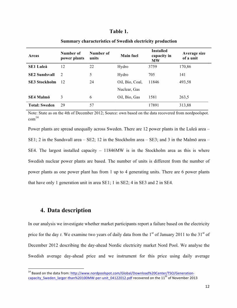
Table 1.
Summary characteristics of Swedish electricity production
Areas Number of power plants
Number of units Main fuel
Installed capacity in MW
Average size of a unit
SE1 Luleå 12 22 Hydro 3759 170,86
SE2 Sundsvall 2 5 Hydro 705 141
SE3 Stockholm 12 24 Oil, Bio, Coal,
Nuclear, Gas
11846 493,58
SE4 Malmö 3 6 Oil, Bio, Gas 1581 263,5
Total: Sweden 29 57 17891 313,88
Note: State as on the 4th of December 2012; Source: own based on the data recovered from nordpoolspot. com14
Power plants are spread unequally across Sweden. There are 12 power plants in the Luleå area –
SE1; 2 in the Sundsvall area – SE2; 12 in the Stockholm area – SE3; and 3 in the Malmö area –
SE4. The largest installed capacity – 11846MW is in the Stockholm area as this is where
Swedish nuclear power plants are based. The number of units is different from the number of
power plants as one power plant has from 1 up to 4 generating units. There are 6 power plants
that have only 1 generation unit in area SE1; 1 in SE2; 4 in SE3 and 2 in SE4.
4. Data description
In our analysis we investigate whether market participants report a failure based on the electricity
price for the day t. We examine two years of daily data from the 1st of January 2011 to the 31st of
December 2012 describing the day-ahead Nordic electricity market Nord Pool. We analyse the
Swedish average day-ahead price and we instrument for this price using daily average
14 Based on the data from: http://www.nordpoolspot.com/Global/Download%20Center/TSO/Generation-‐capacity_Sweden_larger-‐than%20100MW-‐per-‐unit_04122012.pdf recovered on the 11th of November 2013
13
temperatures in Sweden. The information on all unplanned failures larger than 100MW and
lasting for more than 60 min are extracted from the Urgent Market Message dataset. The price
data and the Urgent Market Messages (UMMs) are available upon request from Nord Pool’s
server. The temperature data comes from the Swedish Meteorological and Hydrological Institute
(SMHI).
4.1.Price and temperature data
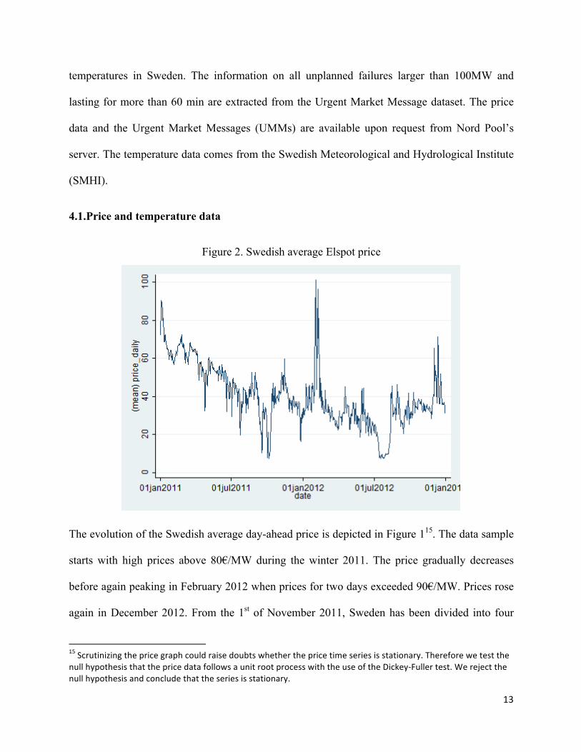
Figure 2. Swedish average Elspot price
The evolution of the Swedish average day-ahead price is depicted in Figure 115. The data sample
starts with high prices above 80€/MW during the winter 2011. The price gradually decreases
before again peaking in February 2012 when prices for two days exceeded 90€/MW. Prices rose
again in December 2012. From the 1st of November 2011, Sweden has been divided into four
15 Scrutinizing the price graph could raise doubts whether the price time series is stationary. Therefore we test the null hypothesis that the price data follows a unit root process with the use of the Dickey-‐Fuller test. We reject the null hypothesis and conclude that the series is stationary.
14
price areas; for the purpose of the analysis in this paper we construct and use an average price for
the whole country. Table 2 reports summary statistics describing price distribution.
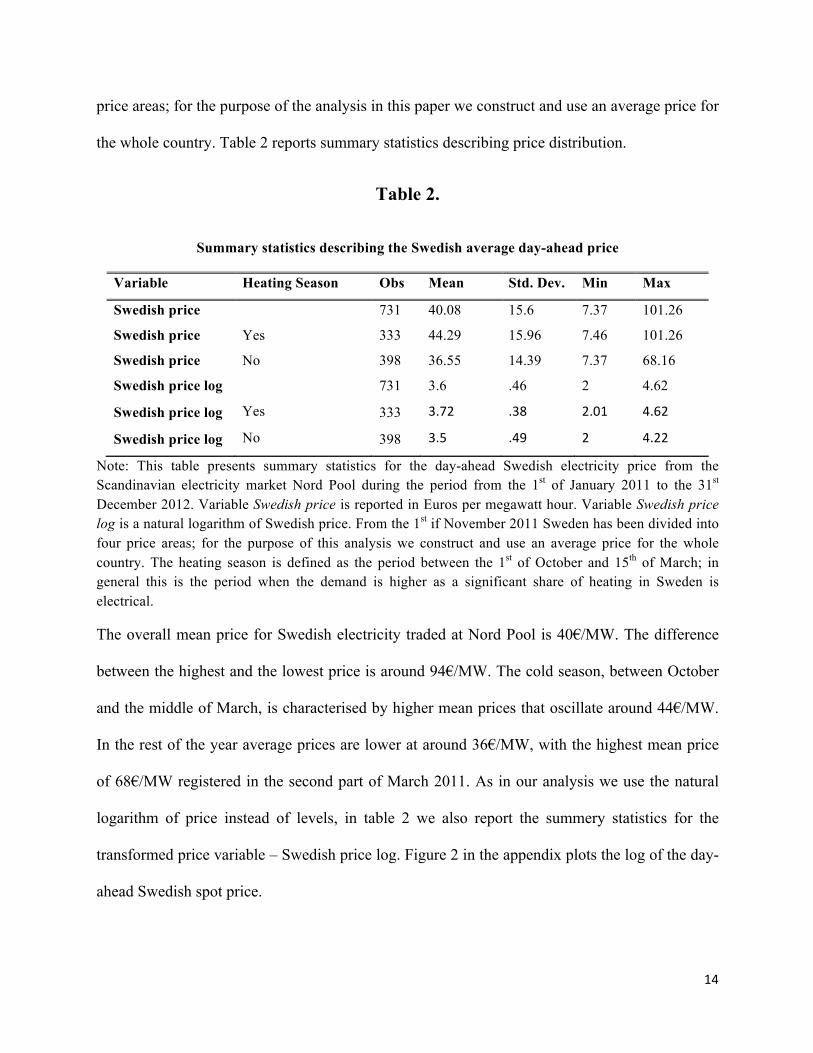
Table 2.
Summary statistics describing the Swedish average day-ahead price
Variable Heating Season Obs Mean Std. Dev. Min Max
Swedish price 731 40.08 15.6 7.37 101.26
Swedish price Yes 333 44.29 15.96 7.46 101.26
Swedish price No 398 36.55 14.39 7.37 68.16
Swedish price log 731 3.6 .46 2 4.62
Swedish price log Yes 333 3.72 .38 2.01 4.62
Swedish price log No 398 3.5 .49 2 4.22
Note: This table presents summary statistics for the day-ahead Swedish electricity price from the Scandinavian electricity market Nord Pool during the period from the 1st of January 2011 to the 31st December 2012. Variable Swedish price is reported in Euros per megawatt hour. Variable Swedish price log is a natural logarithm of Swedish price. From the 1st if November 2011 Sweden has been divided into four price areas; for the purpose of this analysis we construct and use an average price for the whole country. The heating season is defined as the period between the 1st of October and 15th of March; in general this is the period when the demand is higher as a significant share of heating in Sweden is electrical.
The overall mean price for Swedish electricity traded at Nord Pool is 40€/MW. The difference
between the highest and the lowest price is around 94€/MW. The cold season, between October
and the middle of March, is characterised by higher mean prices that oscillate around 44€/MW.
In the rest of the year average prices are lower at around 36€/MW, with the highest mean price
of 68€/MW registered in the second part of March 2011. As in our analysis we use the natural
logarithm of price instead of levels, in table 2 we also report the summery statistics for the
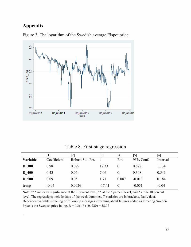
transformed price variable – Swedish price log. Figure 2 in the appendix plots the log of the day-
ahead Swedish spot price.

15
In our analysis we use an average temperature for Sweden to instrument for the price. The mean
temperature in the analysed period is 4.26 Celsius. The coldest period was in February 2011
when the average temperature dropped to -20 Celsius. Table 3 presents summary statistics for the
temperature data.
Table 3.
Summary statistics describing the Swedish average temperature
Variable Obs Mean Std. Dev. Min Max
Temperature 731 4.26 8.16 -21.18 19.56
Note: This table presents summary statistics for the Swedish average temperature recorded between the 1st of January 2011 and the 31st December 2012.
There is an expected negative correlation of -0.47 between the price variable and the temperature
indicating that when the temperature drops the electricity price increases.
4.2. The UMM dataset
The Urgent Market Messages dataset is composed of messages informing about all planned and
unplanned outages exceeding 100MW and lasting for more than 60 min that were recorded in the
Nord Pool area. We measure the number of failures i.e. the unplanned outages per day with the
Failuret variable. Based on the information extracted from the UMMs we are able to identify the
area that is potentially going to be most affected by the event that the message is informing
about. The affected area is identified by the issuer of the message. In our two-year sample there
were 1327 messages announcing failures affecting Sweden; out of these 618 were hydro failures,
341 were nuclear failures, 99 were gas failures, 75 were oil failures, 41 were biofuel failures and
only 4 were coal production failures.

16
In the Nordic area as it gets colder the demand for electricity rises. The calendar year can be
roughly divided into two seasons: the heating season from 1st of October to 15th of March, and
the warmer season without heating covering the rest of the year. As the demand increases, the
production required to meet this demand rises too. Marginal types of production are not
constantly employed but are started when the high level of demand requires additional capacity.
Therefore it is possible that certain types of production report unplanned outages only in winter
when the heating is turned on. To show that this is not the case we report the numbers of
registered messages informing about failures during the heating season (when prices are in
general high) and off the heating season (when prices on average low) in table 4.
Table 4.
Number of messages reporting failures per fuel type
Variable Heating Season Off Heating Season Whole year
Nuclear failure 151 190 341
Hydro failure 333 285 618
Coal failure 4 0 4
Oil failure 56 19 75
Gas failure 58 41 99
Biofuel failure 29 12 41
Note: The heating season is defined as the period between the 1st of October and 15th of March. Last column is the summation of all messages of different fuel type over the studied sample.
The data in the above table indicates that failure messages were reported in both seasons with the
exception of coal fueled electricity generation that has issued only 4 messages informing about
problems affecting Sweden. Subsequently we drop coal failures from the further analysis.
17
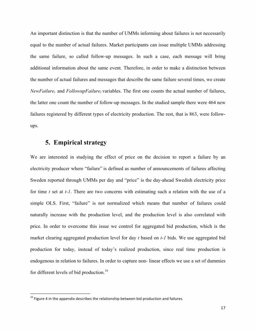
An important distinction is that the number of UMMs informing about failures is not necessarily
equal to the number of actual failures. Market participants can issue multiple UMMs addressing
the same failure, so called follow-up messages. In such a case, each message will bring
additional information about the same event. Therefore, in order to make a distinction between
the number of actual failures and messages that describe the same failure several times, we create
NewFailuret and FollowupFailuret variables. The first one counts the actual number of failures,
the latter one count the number of follow-up messages. In the studied sample there were 464 new
failures registered by different types of electricity production. The rest, that is 863, were follow-
ups.
5. Empirical strategy
We are interested in studying the effect of price on the decision to report a failure by an
electricity producer where “failure” is defined as number of announcements of failures affecting
Sweden reported through UMMs per day and “price” is the day-ahead Swedish electricity price
for time t set at t-1. There are two concerns with estimating such a relation with the use of a
simple OLS. First, “failure” is not normalized which means that number of failures could
naturally increase with the production level, and the production level is also correlated with
price. In order to overcome this issue we control for aggregated bid production, which is the
market clearing aggregated production level for day t based on t-1 bids. We use aggregated bid
production for today, instead of today’s realized production, since real time production is
endogenous in relation to failures. In order to capture non- linear effects we use a set of dummies
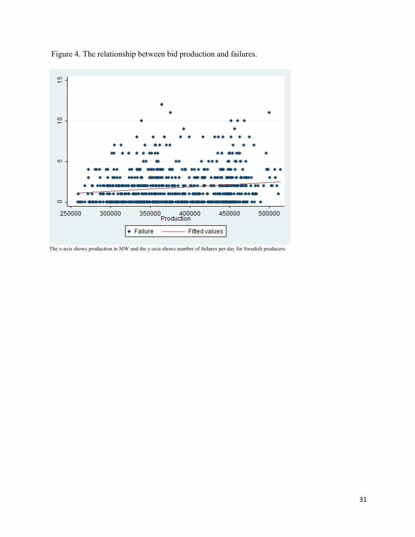
for different levels of bid production.16
16 Figure 4 in the appendix describes the relationship between bid production and failures.

18
Second, in an OLS regression we require that 𝐸 𝑒𝑟𝑟𝑜𝑟_𝑡𝑒𝑟𝑚! 𝑃𝑟𝑖𝑐𝑒! = 0. However, even
though 𝑃𝑟𝑖𝑐𝑒! is set on the day before failure is reported, there is a clear risk that different
omitted variables such as market players’ bidding strategies or technical considerations affect
both prices set yesterday and number of failures today. For instance high prices could encourage
producers to run their generators above recommended capacity levels which would increase the
risk of failures. We hence instrument for prices using daily average temperature for Sweden in a
two-stage model. Both stages are described below.
First stage:
𝐿𝑜𝑔𝑃𝑟𝑖𝑐𝑒! = 𝛽!𝑇𝑒𝑚𝑝𝑒𝑟𝑎𝑡𝑢𝑟𝑒! + 𝛽!! !!!! 𝐵𝑖𝑑𝑃𝑟𝑜𝑑𝑢𝑐𝑡𝑖𝑜𝑛! + 𝛾!𝑊!+ 𝜖!!
!!! (1)
Second stage:
𝐿𝑜𝑔𝐹𝑎𝑖𝑙𝑢𝑟𝑒! = 𝛽!𝐿𝑜𝑔𝑃𝑟𝚤𝑐𝑒! + 𝛽!! !!!!
𝐵𝑖𝑑𝑃𝑟𝑜𝑑𝑢𝑐𝑡𝑖𝑜𝑛! + 𝛿!𝑊!+ 𝜀!!!!! (2)
The key identifying assumption in order for our instrument to be valid is that
𝐸 𝜖! 𝑇𝑒𝑚𝑝𝑒𝑟𝑎𝑡𝑢𝑟𝑒! ,𝐵𝑖𝑑𝑃𝑟𝑜𝑑𝑢𝑐𝑡𝑖𝑜𝑛! ,𝑊! = 0 . Conditioned on the control variables, there
should be no correlation between temperature and the error term in the equation we wish to
correctly estimate (equation 1). This condition should be satisfied since temperature is strictly
exogenous. It is also necessary that there is no direct effect of temperature on the probability of
production failures. In the studied period we did not observe any extreme temperatures that
would be unfamiliar to Scandinavia. Power plants in the Nordic Region are constructed with the
aim of withstanding the normal weather conditions and should not be affected by a normal range
of temperatures. The only potential link between the temperature and failures can be attributed to
freezing of water reservoirs, which potentially increases the probability of failure of hydro-fueled
generators. However, since every UMM contains a description of the reported problem we can
19
manually remove all messages that would indicate that the outage was caused by special weather
conditions, for instance freezing.
Results of the first stage regression (eq. 1) are reported in Table 8 in the appendix. The high F-
statistic of 38 indicates that the temperature is significant and can be used as an instrument for
prices.
5.1 Analysis of all messages
Our baseline estimation equations are equations 1 and 2 above. The dependent variable is the log
of the number of failure messages issued at day t17. We use BidProductiont dummies for
normalization purposes. To capture weekly demand patterns we use weekday dummies. Our
variable of interest is LogPricet.
As we believe that producers using different production fuels and therefore occupying different
places in the merit order have different incentives for withholding we divide the dependent
variable Failuret into messages informing about different fuels. We therefore create five
dependent variables that count number of messages issued by nuclear, hydro, oil, gas and
biofuel-fuel generators every day. In the analysis we turn these variables into log-variables. We
repeat the estimation strategy described in equations 1 and 2 for those five new dependent
variables.
5.2 Analysis of new and follow-up messages
In order to test whether economic incentives affect the timing of new failures or if economic
incentives primarily affect the duration of maintenance after a failure we repeat our two-step
17 We transform the original count variable by adding 1 in order to be able to take the log. This is a standard way of transforming a count variable with many zeroes.
20
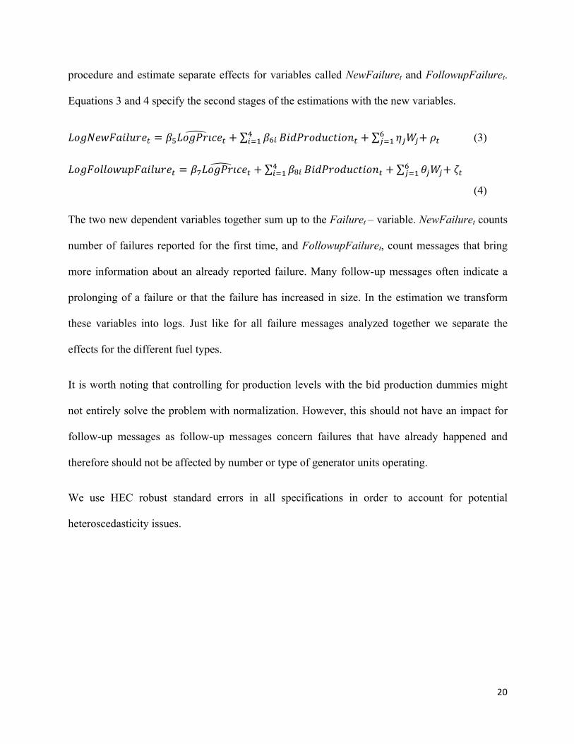
procedure and estimate separate effects for variables called NewFailuret and FollowupFailuret.
Equations 3 and 4 specify the second stages of the estimations with the new variables.
𝐿𝑜𝑔𝑁𝑒𝑤𝐹𝑎𝑖𝑙𝑢𝑟𝑒! = 𝛽!𝐿𝑜𝑔𝑃𝑟𝚤𝑐𝑒! + 𝛽!! !!!! 𝐵𝑖𝑑𝑃𝑟𝑜𝑑𝑢𝑐𝑡𝑖𝑜𝑛! + 𝜂!𝑊!+ 𝜌!!
!!! (3)
𝐿𝑜𝑔𝐹𝑜𝑙𝑙𝑜𝑤𝑢𝑝𝐹𝑎𝑖𝑙𝑢𝑟𝑒! = 𝛽!𝐿𝑜𝑔𝑃𝑟𝚤𝑐𝑒! + 𝛽!! !!!! 𝐵𝑖𝑑𝑃𝑟𝑜𝑑𝑢𝑐𝑡𝑖𝑜𝑛! + 𝜃!𝑊!+ 𝜁!!
!!!
(4)
The two new dependent variables together sum up to the Failuret – variable. NewFailuret counts
number of failures reported for the first time, and FollowupFailuret, count messages that bring
more information about an already reported failure. Many follow-up messages often indicate a
prolonging of a failure or that the failure has increased in size. In the estimation we transform
these variables into logs. Just like for all failure messages analyzed together we separate the
effects for the different fuel types.
It is worth noting that controlling for production levels with the bid production dummies might
not entirely solve the problem with normalization. However, this should not have an impact for
follow-up messages as follow-up messages concern failures that have already happened and
therefore should not be affected by number or type of generator units operating.
We use HEC robust standard errors in all specifications in order to account for potential
heteroscedasticity issues.
21
6. Results
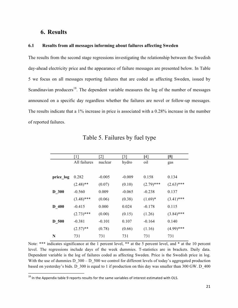
6.1 Results from all messages informing about failures affecting Sweden
The results from the second stage regressions investigating the relationship between the Swedish
day-ahead electricity price and the appearance of failure messages are presented below. In Table
5 we focus on all messages reporting failures that are coded as affecting Sweden, issued by
Scandinavian producers18. The dependent variable measures the log of the number of messages
announced on a specific day regardless whether the failures are novel or follow-up messages.
The results indicate that a 1% increase in price is associated with a 0.28% increase in the number
of reported failures.
Table 5. Failures by fuel type
[1] [2] [3] [4] [5] All failures nuclear hydro oil gas
price_log 0.282 -0.005 -0.009 0.158 0.134
(2.48)** (0.07) (0.10) (2.79)*** (2.63)***
D_300 -0.560 0.009 -0.065 -0.238 0.137
(3.48)*** (0.06) (0.38) (1.69)* (3.41)***
D_400 -0.415 0.000 0.024 -0.178 0.115
(2.73)*** (0.00) (0.15) (1.26) (3.84)***
D_500 -0.381 -0.101 0.107 -0.164 0.140
(2.57)** (0.78) (0.66) (1.16) (4.99)***
N 731 731 731 731 731
Note: *** indicates significance at the 1 percent level, ** at the 5 percent level, and * at the 10 percent level. The regressions include days of the week dummies. T-statistics are in brackets. Daily data. Dependent variable is the log of failures coded as affecting Sweden. Price is the Swedish price in log. With the use of dummies D_300 – D_500 we control for different levels of today’s aggregated production based on yesterday’s bids. D_300 is equal to 1 if production on this day was smaller than 300 GW. D_400 18 In the Appendix table 9 reports results for the same variables of interest estimated with OLS.
22
is equal to 1 if production was larger than 300 GW but smaller than 400 GW. Price is instrumented with temperature.
As we assume that particular technologies used for producing electricity might face different
incentives, we disaggregate the failures into outages reported by different fuel types. There are
positive and significant results for gas and oil, where a 1 % increase in price increases the
number of reported failures by 0.134 % in case of gas fueled generation and by 0.16 % in the
case of oil. There are no significant effects for nuclear or hydro.
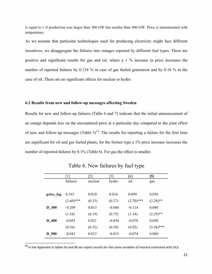
6.2 Results from new and follow-up messages affecting Sweden
Results for new and follow-up failures (Table 6 and 7) indicate that the initial announcement of
an outage depends less on the encountered price at a particular day compared to the joint effect
of new and follow-up messages (Table 5)19. The results for reporting a failure for the first time
are significant for oil and gas fueled plants, for the former type a 1% price increase increases the
number of reported failures by 0.1% (Table 6). For gas the effect is smaller.
Table 6. New failures by fuel type
[1] [2] [3] [4] [5] failures nuclear hydro oil gas
price_log 0.193 0.010 0.016 0.099 0.058
(2.60)*** (0.33) (0.27) (2.70)*** (2.28)**
D_300 -0.209 0.013 -0.086 -0.114 0.040
(1.34) (0.19) (0.75) (1.34) (2.29)**
D_400 -0.055 0.021 -0.034 -0.078 0.050
(0.36) (0.32) (0.30) (0.92) (3.56)***
D_500 -0.041 0.013 -0.013 -0.074 0.060
19 In the Appendix in tables 9a and 9b we report results for the same variables of interest estimated with OLS.
23
(0.27) (0.20) (0.12) (0.87) (4.50)***
N 731 731 731 731 731
Note: *** indicates significance at the 1 percent level, ** at the 5 percent level, and * at the 10 percent level. The regressions include days of the week dummies. T-statistics are in brackets. Daily data. Dependent variable is the log of novel messages informing about failures coded as affecting Sweden. Price is the Swedish price in log. With the use of dummies D_300 – D_500 we control for different levels of today’s aggregated production based on yesterday’s bids. D_300 is equal to 1 if production on this day was smaller than 300 GW. D_400 is equal to 1 if production was larger than 300 GW but smaller than 400 GW. Price is instrumented with temperature.
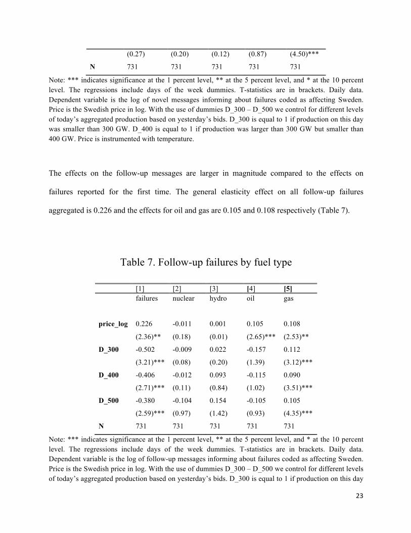
The effects on the follow-up messages are larger in magnitude compared to the effects on
failures reported for the first time. The general elasticity effect on all follow-up failures
aggregated is 0.226 and the effects for oil and gas are 0.105 and 0.108 respectively (Table 7).
Table 7. Follow-up failures by fuel type
[1] [2] [3] [4] [5] failures nuclear hydro oil gas
price_log 0.226 -0.011 0.001 0.105 0.108
(2.36)** (0.18) (0.01) (2.65)*** (2.53)**
D_300 -0.502 -0.009 0.022 -0.157 0.112
(3.21)*** (0.08) (0.20) (1.39) (3.12)***
D_400 -0.406 -0.012 0.093 -0.115 0.090
(2.71)*** (0.11) (0.84) (1.02) (3.51)***
D_500 -0.380 -0.104 0.154 -0.105 0.105
(2.59)*** (0.97) (1.42) (0.93) (4.35)***
N 731 731 731 731 731
Note: *** indicates significance at the 1 percent level, ** at the 5 percent level, and * at the 10 percent level. The regressions include days of the week dummies. T-statistics are in brackets. Daily data. Dependent variable is the log of follow-up messages informing about failures coded as affecting Sweden. Price is the Swedish price in log. With the use of dummies D_300 – D_500 we control for different levels of today’s aggregated production based on yesterday’s bids. D_300 is equal to 1 if production on this day

24
was smaller than 300 GW. D_400 is equal to 1 if production was larger than 300 GW but smaller than 400 GW. Price is instrumented with temperature.
These findings confirm our hypothesis that the economic incentives are more important when
deciding on the scope of a failure, that is, the size and duration of the failure measured through
follow-up messages as compared to the decision of whether to report a new failure.
The effects for both scenarios that we test do not indicate that economic incentives matter for
reporting failures in the case of the baseload production. The results for both nuclear and hydro
generation are not significant. This finding is not surprising since due to low marginal costs the
baseload production can recover high infra-marginal profits if the electricity price is established
by the marginal units. Reporting a failure when other, more expensive, types of production set
the price is not in the economic interest of a cheap producer.
7. Conclusions
In this paper we investigate whether producers supplying electricity to the Swedish market base
their decision of whether to report a failure on economic incentives or on purely technical
reasons. The results indicate that prices affect failures reported through Urgent Market Messages
in different ways depending on the type of electricity generation. We find no significant effects
for the baseload technologies, that is, nuclear and hydro, which suggests that failure risks for
baseload technologies do not depend on daily variations in spot prices. However, we do observe
a positive and significant effect of spot prices on the number of reported failures in the case of
marginal production generators, which in the case of Sweden are oil and gas.
These findings support the hypothesis that economic incentives play a role when marginal
producers decide to report a failure. Small changes to marginal production in periods of high
25
demand can have potentially larger effect on the price levels as compared with similar changes
of baseload production in low demand periods. Moreover, producers who own both types of
electricity generation: infra-marginal and marginal are interested in recovering high infra-
marginal profits while at the same time decreasing production costs. A strategy to withdraw
expensive marginal capacity disguising it as a failure could accomplish these goals.
We see that the effect on follow-up messages is slightly larger in magnitude compared to the
effect on failures reported for the first time. This indicates that economic incentives might to a
greater degree affect the duration of a failure compared to the probability of reporting a new
failure.
References
Crampes, C., Creti, A., 2005, Capacity competition in electricity markets, Economia delle fonti di energia e dell'ambiente v, p.59-83.
Fridolfsson, S., Tangeras, T., 2009, Market power in the Nordic electricity wholesale market: A survey of the empirical evidence, Research Institute of Industrial Economics, April 17, 2009.
Green, R., 2004, Did English generators play Cournot? Capacity withholding in the Electricity Pool, Working Paper 04-010 WP, Center for Energy and Environmental Policy Research.
Hjalmarsson, E., 2000, Nord Pool: A power market without market power, Discussion Paper No. 28, Gothenburg University.
Kwoka, J. and Sabodash, V., 2011, Price spikes in energy markets: “Business by usual methods” or strategic withholding?, Review of Industrial Organization, 38, 285-310.
Kwoka, J., 2012, Price spikes in wholesale electricity markets: an update on problems and policies, Conference on Pressing Issues in World Energy Policy, University of Florida.
Moss, D.L., 2006, Electricity and market power: Current issues for restructuring markets, Environmental & Enery Law & Policy Journal, 1 (1), pp 11-41.
Newbery, D., 1995, Power Markets and Market Power, The Energy Journal, Vol 16, No
26
3, pp 39-66.
Nord Pool, 2012, Annual report.
Vassilopoulous, P., 2003, Models for identification of market power in wholesale electricity markets, Graduate thesis, University of Paris IX.
Weaver, J., 2004, Can energy markets be trusted? The effect of the rise and fall of Enron on energy markets, Houston Business and Tax Law Journal, (4).
Wolfram, C., 1998, Strategic bidding in a multi-unit auction: an empirical analysis of bids to supply electricity in England and Wales, RAND Journal of Economics, vol 29, no 4, pp 703-725.
Wolfram, C., 1999, Measuring duopoly power in the British electricity spot market, American Economic Review, 89, 805-826.
27
Appendix
Figure 3. The logarithm of the Swedish average Elspot price
Table 8. First-stage regression
[1] [2] [3] [4] [5] [6] Variable Coefficient Robust Std. Err. t P>t 95% Conf. Interval
D_300 0.98 0.079 12.33 0 0.822 1.134
D_400 0.43 0.06 7.06 0 0.308 0.546
D_500 0.09 0.05 1.71 0.087 -0.013 0.184
temp -0.05 0.0026 -17.41 0 -0.051 -0.04
Note: *** indicates significance at the 1 percent level, ** at the 5 percent level, and * at the 10 percent level. The regressions include days of the week dummies. T-statistics are in brackets. Daily data. Dependent variable is the log of follow-up messages informing about failures coded as affecting Sweden. Price is the Swedish price in log. R = 0.36; F (10, 720) = 38.07
.

28
Table 9. Failures by fuel type - OLS
[1] [2] [3] [4] [5]
failure nuclear hydro oil gas
price_log -0.016 -0.096 -0.070 0.056 0.065
(0.25) (2.14)** (1.40) (2.43)** (2.73)***
D_400 0.053 -0.036 0.071 0.028 -0.043
(0.62) (0.55) (1.00) (1.16) (1.09)
D_500 0.142 -0.121 0.165 0.062 -0.005
(1.63) (1.80)* (2.27)** (2.32)** (0.13)
D_600 0.589 0.000 0.071 0.248 -0.130
(3.69)*** (0.00) (0.41) (1.73)* (3.21)***
R2 0.05 0.04 0.04 0.05 0.03
N 731 731 731 731 731
Note: *** indicates significance at the 1 percent level, ** at the 5 percent level, and * at the 10 percent level. The regressions include days of the week dummies. T-statistics are in brackets. Daily data. Dependent variable is the log of number of messages informing about failures coded as affecting Sweden. Price is the Swedish price in log. OLS regression.
Table 9a. New failures by fuel type - OLS [1] [2] [3] [4] [5]
failure nuclear hydro oil gas
price_log 0.007 -0.020 -0.040 0.033 0.031
(0.17) (1.02) (1.23) (2.26)** (2.63)***
D_300 -0.228 0.010 -0.091 -0.120 0.037
(1.44) (0.15) (0.80) (1.38) (2.10)**
D_400 -0.131 0.009 -0.056 -0.104 0.039
(0.86) (0.14) (0.52) (1.22) (3.66)***
D_500 -0.083 0.006 -0.025 -0.088 0.054
(0.54) (0.09) (0.23) (1.02) (4.74)***
R2 0.03 0.01 0.02 0.03 0.02
N 731 731 731 731 731
Note: *** indicates significance at the 1 percent level, ** at the 5 percent level, and * at the 10 percent level. The regressions include days of the week dummies. T-statistics are in brackets. Daily data. Dependent variable is the log of new messages informing about failures coded as affecting Sweden. Price is the Swedish price in log. OLS regression.
29
Table 9b. Follow-up failures by fuel type - OLS
[1] [2] [3] [4] [5]
failure nuclear hydro oil gas
price_log -0.019 -0.087 -0.051 0.040 0.051
(0.37) (2.12)** (1.41) (2.46)** (2.52)**
D_300 -0.526 -0.017 0.017 -0.163 0.106
(3.39)*** (0.14) (0.15) (1.43) (2.94)***
D_400 -0.505 -0.043 0.072 -0.142 0.067
(3.49)*** (0.40) (0.66) (1.25) (3.52)***
D_500 -0.435 -0.121 0.143 -0.120 0.093
(3.01)*** (1.14) (1.31) (1.06) (4.43)***
R2 0.06 0.04 0.04 0.05 0.04
N 731 731 731 731 731
Note: *** indicates significance at the 1 percent level, ** at the 5 percent level, and * at the 10 percent level. The regressions include days of the week dummies. T-statistics are in brackets. Daily data. Dependent variable is the log of follow-up messages informing about failures coded as affecting Sweden. Price is the Swedish price in log. OLS regression.
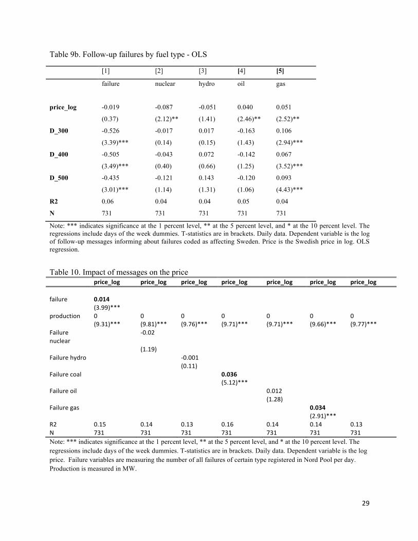
Table 10. Impact of messages on the price price_log price_log price_log price_log price_log price_log price_log failure 0.014 (3.99)*** production 0 0 0 0 0 0 0 (9.31)*** (9.81)*** (9.76)*** (9.71)*** (9.71)*** (9.66)*** (9.77)*** Failure nuclear
-‐0.02
(1.19) Failure hydro -‐0.001 (0.11) Failure coal 0.036 (5.12)*** Failure oil 0.012 (1.28) Failure gas 0.034 (2.91)*** R2 0.15 0.14 0.13 0.16 0.14 0.14 0.13 N 731 731 731 731 731 731 731 Note: *** indicates significance at the 1 percent level, ** at the 5 percent level, and * at the 10 percent level. The regressions include days of the week dummies. T-statistics are in brackets. Daily data. Dependent variable is the log price. Failure variables are measuring the number of all failures of certain type registered in Nord Pool per day. Production is measured in MW.
30
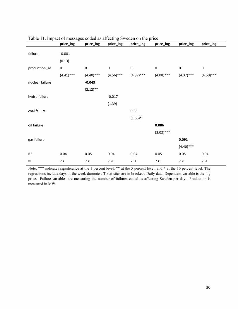
Table 11. Impact of messages coded as affecting Sweden on the price price_log price_log price_log price_log price_log price_log price_log failure -‐0.001
(0.13)
production_se 0 0 0 0 0 0 0
(4.41)*** (4.40)*** (4.56)*** (4.37)*** (4.08)*** (4.37)*** (4.50)***
nuclear failure -‐0.043
(2.12)**
hydro failure -‐0.017
(1.39)
coal failure 0.33
(1.66)*
oil failure 0.086
(3.02)***
gas failure 0.091
(4.40)***
R2 0.04 0.05 0.04 0.04 0.05 0.05 0.04
N 731 731 731 731 731 731 731
Note: *** indicates significance at the 1 percent level, ** at the 5 percent level, and * at the 10 percent level. The regressions include days of the week dummies. T-statistics are in brackets. Daily data. Dependent variable is the log price. Failure variables are measuring the number of failures coded as affecting Sweden per day. Production is measured in MW.
31
Figure 4. The relationship between bid production and failures.
The x-axis shows production in MW and the y-axis shows number of failures per day for Swedish producers.