Embed Size (px)
Citation preview
Nahum ShimkinDepartment of Electrical Engineering
Technion
Workshop on Congestion Games IMS/NUS, Singapore, December 2015
Strategic Timing Decisionsin Service Systems
Games of Timing
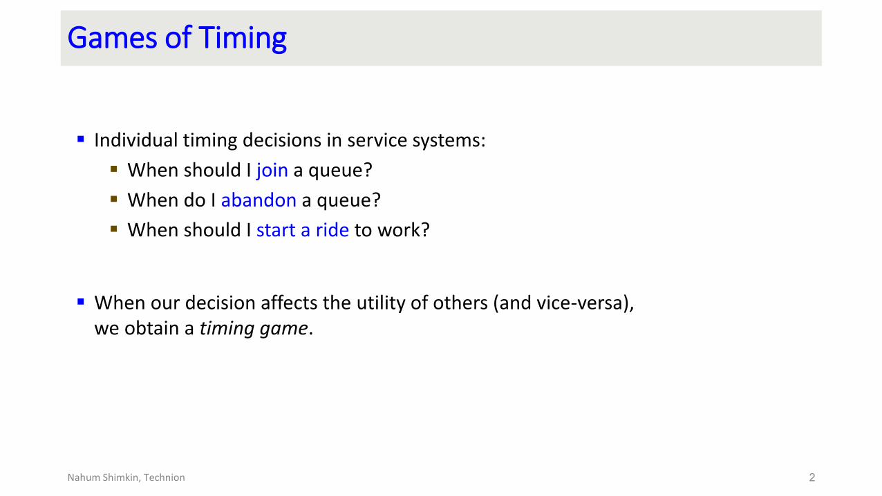
Individual timing decisions in service systems:
When should I join a queue?
When do I abandon a queue?
When should I start a ride to work?
When our decision affects the utility of others (and vice-versa), we obtain a timing game.
2Nahum Shimkin, Technion
Nahum Shimkin, Technion3
Abandonment Decisions
Rational Abandonments from Invisible Queues [with Avishai Mandelbaum: 2000, 2004]
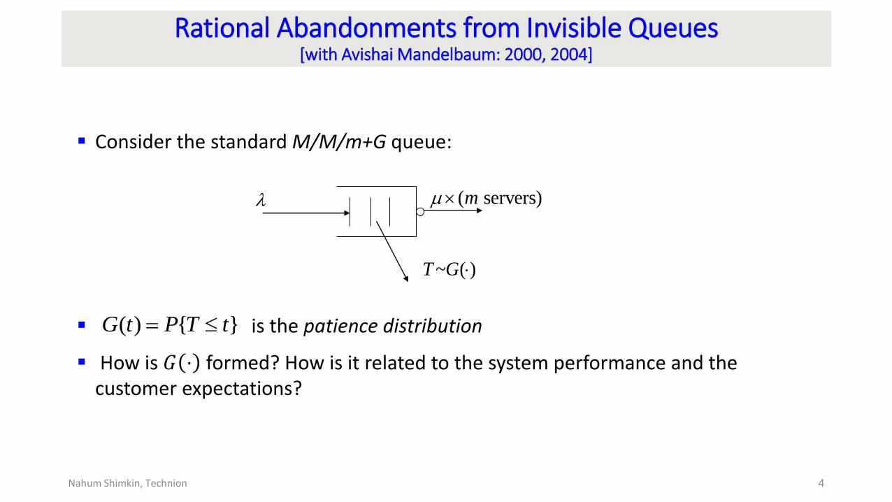
Consider the standard M/M/m+G queue:
is the patience distribution
How is 𝐺 ⋅ formed? How is it related to the system performance and the customer expectations?
4Nahum Shimkin, Technion
( servers)m
~ ( )T G
( ) { }G t P T t
Empirical Observations
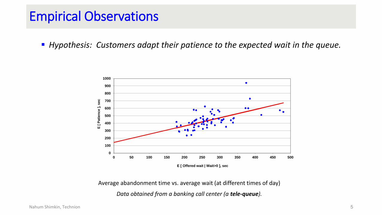
Hypothesis: Customers adapt their patience to the expected wait in the queue.
5Nahum Shimkin, Technion
Average abandonment time vs. average wait (at different times of day)
Data obtained from a banking call center (a tele-queue).
0
100
200
300
400
500
600
700
800
900
1000
0 50 100 150 200 250 300 350 400 450 500
E [
Pa
tie
nc
e ]
, s
ec
E [ Offered wait | Wait>0 ], sec
Rational Abandonment Model
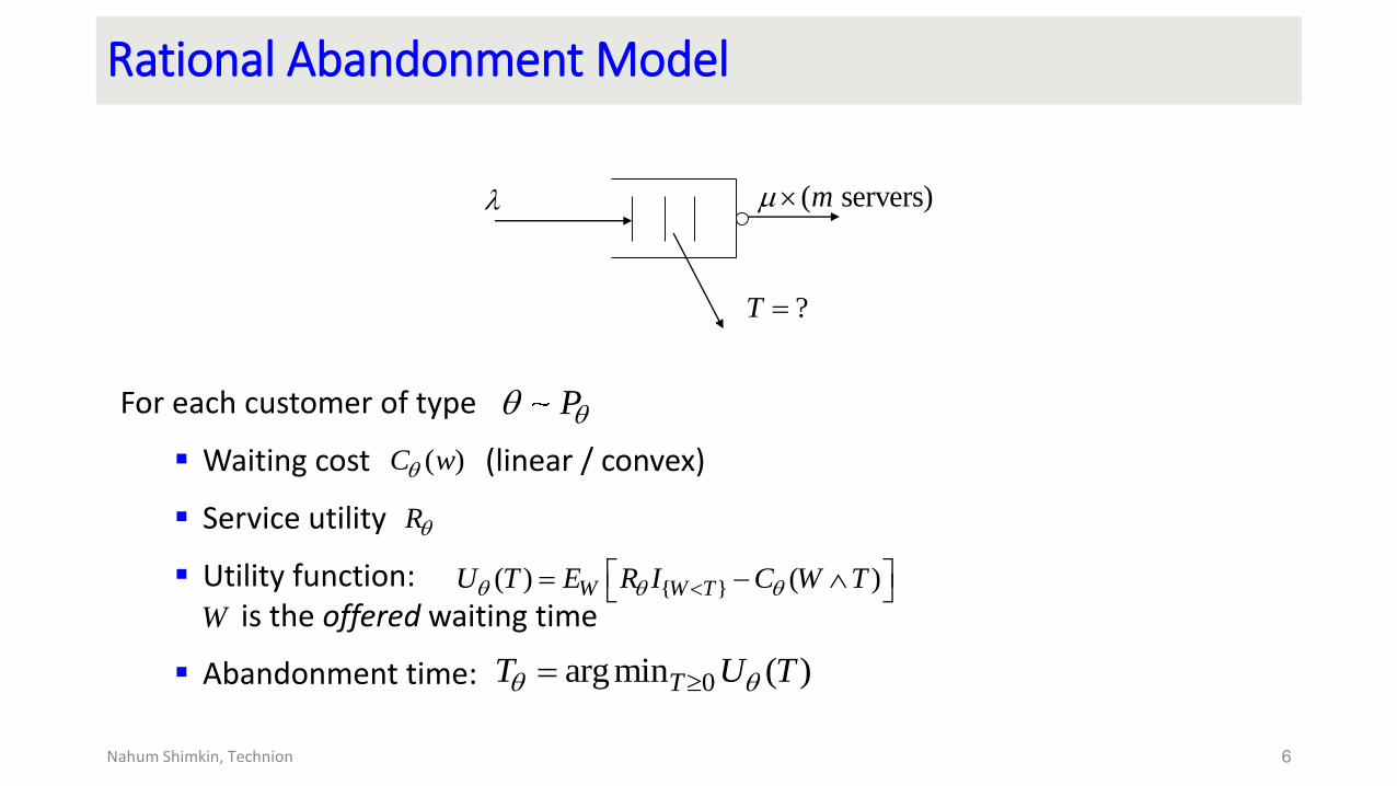
For each customer of type
Waiting cost (linear / convex)
Service utility
Utility function: is the offered waiting time
Abandonment time:
6Nahum Shimkin, Technion
( )C w
R
{ }( ) ( )W W TU T E R I C W T
W
P
( servers)m
?T
0argmin ( )TT U T
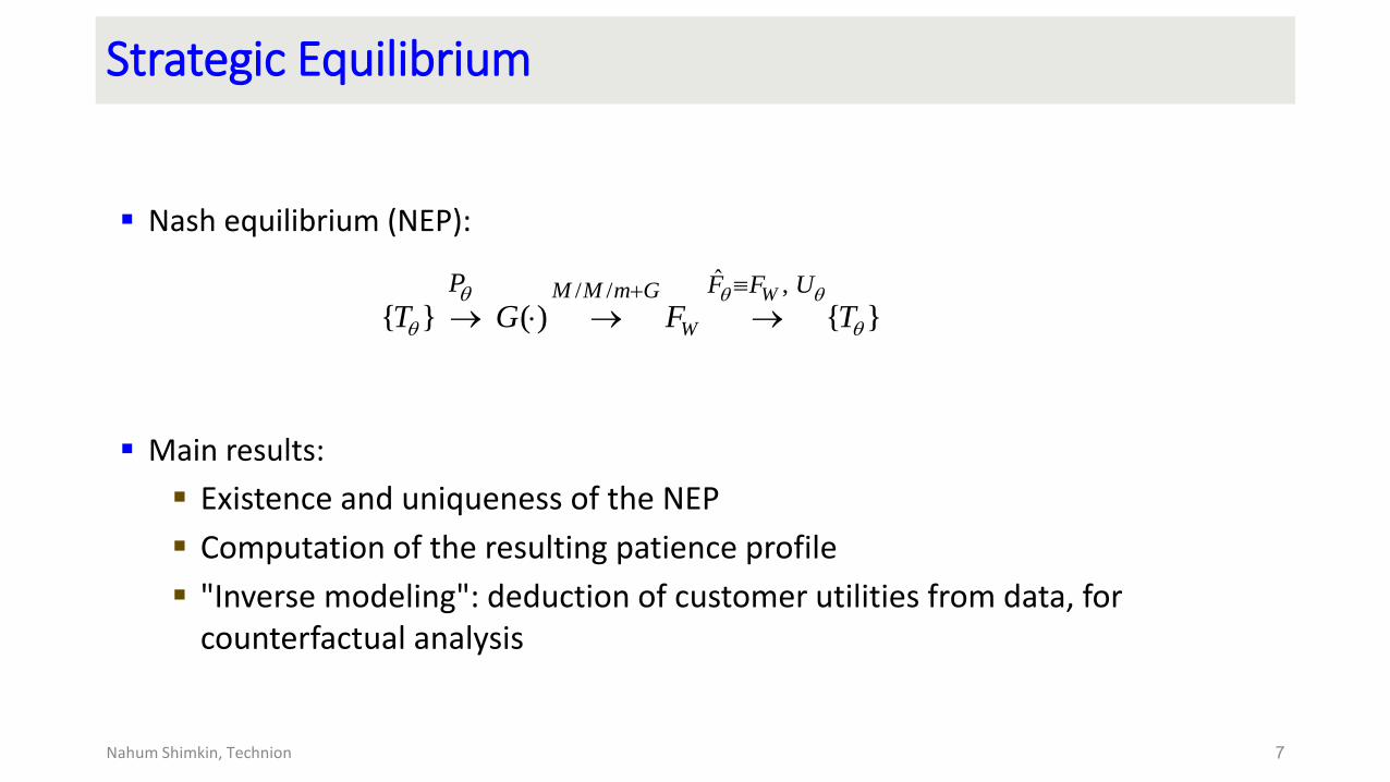
Strategic Equilibrium
Nash equilibrium (NEP):
Main results:
Existence and uniqueness of the NEP
Computation of the resulting patience profile
"Inverse modeling": deduction of customer utilities from data, for counterfactual analysis
7Nahum Shimkin, Technion
/ /ˆ ,
{ } ( ) { }W
W
M M m G F F UP
T G F T
Nahum Shimkin, Technion8
Arrival Time Decisions
Strategic Choice of Arrival Times in Transient Queues
With Sandeep Juneja and Rahul Jain: 2011,2013
The model:
A FCFS service system that starts serving at time 0
A finite population (possibly of random size) of customers
Each customer may choose his or her arrival time to the queue
9Nahum Shimkin, Technion
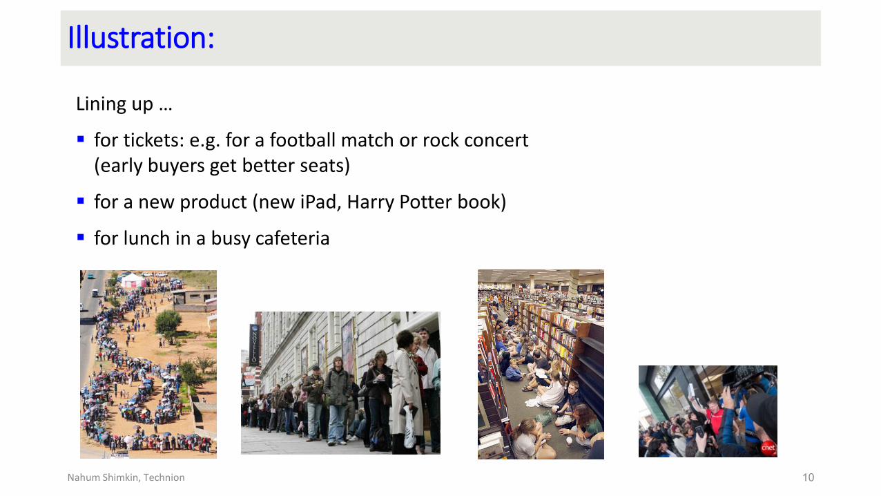
Illustration:
Lining up …
for tickets: e.g. for a football match or rock concert (early buyers get better seats)
for a new product (new iPad, Harry Potter book)
for lunch in a busy cafeteria
10Nahum Shimkin, Technion
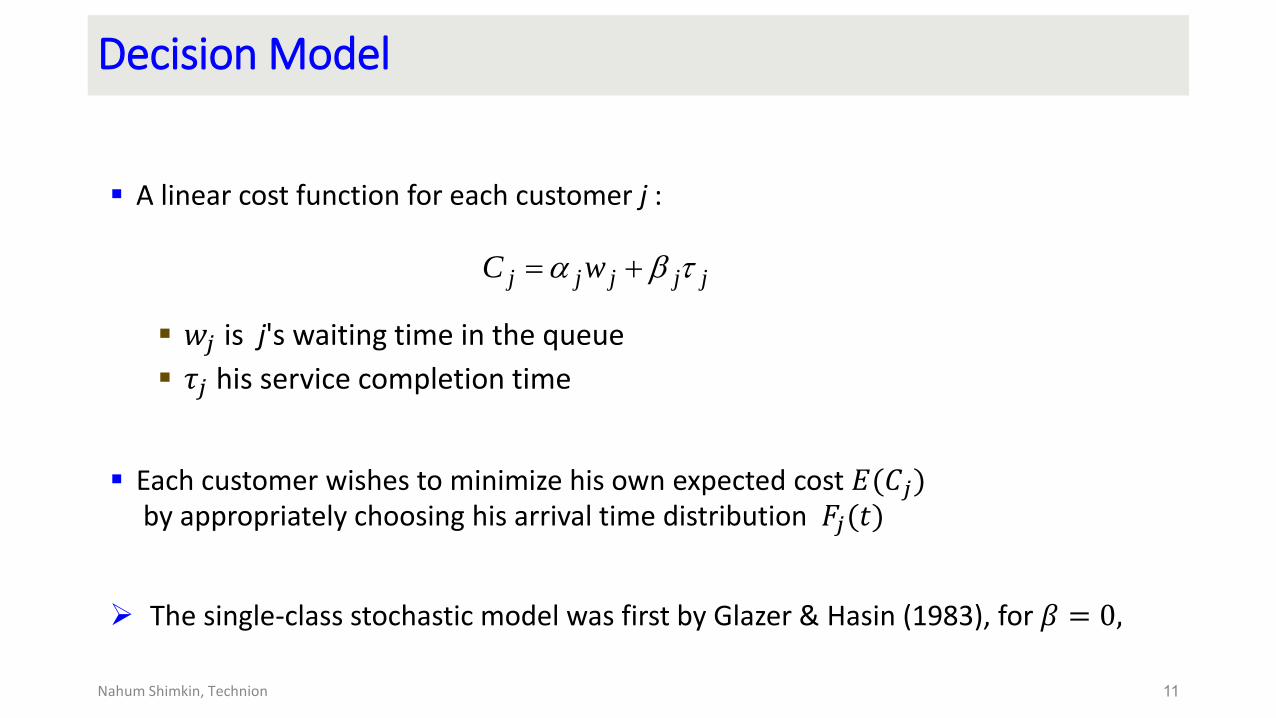
Decision Model
A linear cost function for each customer j :
𝑤𝑗 is j's waiting time in the queue
𝜏𝑗 his service completion time
Each customer wishes to minimize his own expected cost 𝐸(𝐶𝑗)by appropriately choosing his arrival time distribution 𝐹𝑗(𝑡)
The single-class stochastic model was first by Glazer & Hasin (1983), for 𝛽 = 0,
11Nahum Shimkin, Technion
j j j j jC w
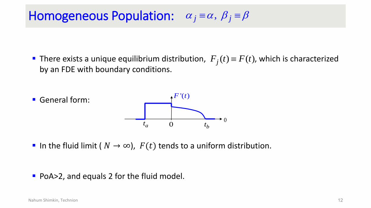
Homogeneous Population:
There exists a unique equilibrium distribution, , which is characterized by an FDE with boundary conditions.
General form:
In the fluid limit ( 𝑁 → ∞), 𝐹(𝑡) tends to a uniform distribution.
PoA>2, and equals 2 for the fluid model.
12Nahum Shimkin, Technion
,j j
( ) ( )jF t F t
00
'( )F t
at bt
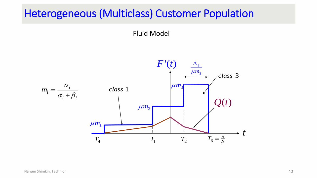
Heterogeneous (Multiclass) Customer Population
Fluid Model
13Nahum Shimkin, Technion
t
'( )F t
3T
1T 2T4T
3class
1m
( )Q t2m
3m
3
3m
1classi
i iim
Nahum Shimkin, Technion14
Timing of Ad Posting
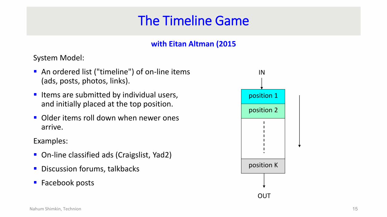
The Timeline Game
with Eitan Altman (2015
System Model:
An ordered list ("timeline") of on-line items(ads, posts, photos, links).
Items are submitted by individual users,and initially placed at the top position.
Older items roll down when newer onesarrive.
Examples:
On-line classified ads (Craigslist, Yad2)
Discussion forums, talkbacks
Facebook posts
15Nahum Shimkin, Technion
position 1
position 2
position K
IN
OUT
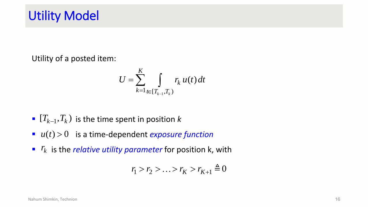
Utility Model
Utility of a posted item:
is the time spent in position k
is a time-dependent exposure function
is the relative utility parameter for position k, with
16Nahum Shimkin, Technion
11 [ , )
( )
k k
K
k
k t T T
U r u t dt
1[ , )k kT T
( ) 0u t
kr
1 2 1 0K Kr r r r
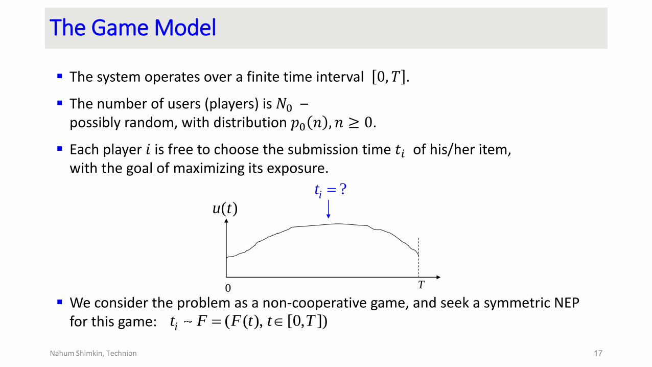
The Game Model
The system operates over a finite time interval 0, 𝑇 .
The number of users (players) is 𝑁0 –possibly random, with distribution 𝑝0 𝑛 , 𝑛 ≥ 0.
Each player 𝑖 is free to choose the submission time 𝑡𝑖 of his/her item,with the goal of maximizing its exposure.
We consider the problem as a non-cooperative game, and seek a symmetric NEP for this game:
17Nahum Shimkin, Technion
( ( ), [0, ])it F F t t T
0 T
( )u t
?it
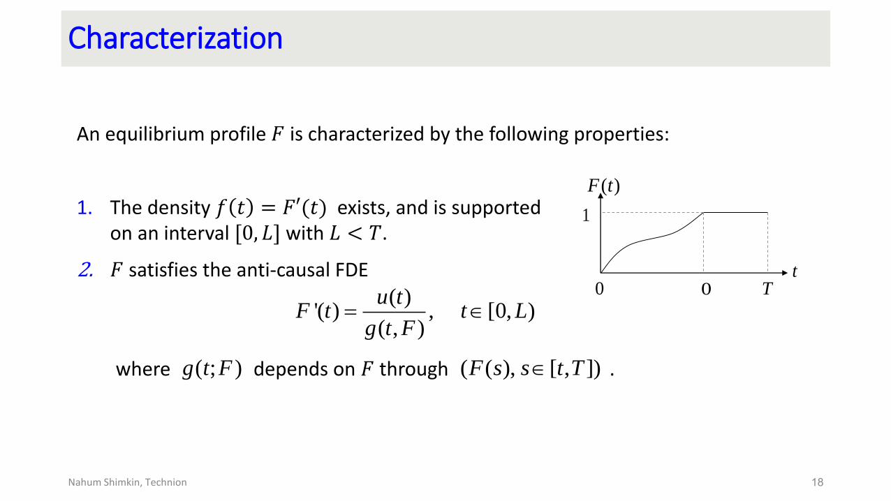
Characterization
An equilibrium profile 𝐹 is characterized by the following properties:
1. The density 𝑓 𝑡 = 𝐹′(𝑡) exists, and is supportedon an interval [0, 𝐿] with 𝐿 < 𝑇.
2. 𝐹 satisfies the anti-causal FDE
where depends on 𝐹 through .
18Nahum Shimkin, Technion
( )'( ) , [0, )
( , )
u tF t t L
g t F
( ; )g t F ( ( ), [ , ])F s s t T
0 T0
1
( )F t
t
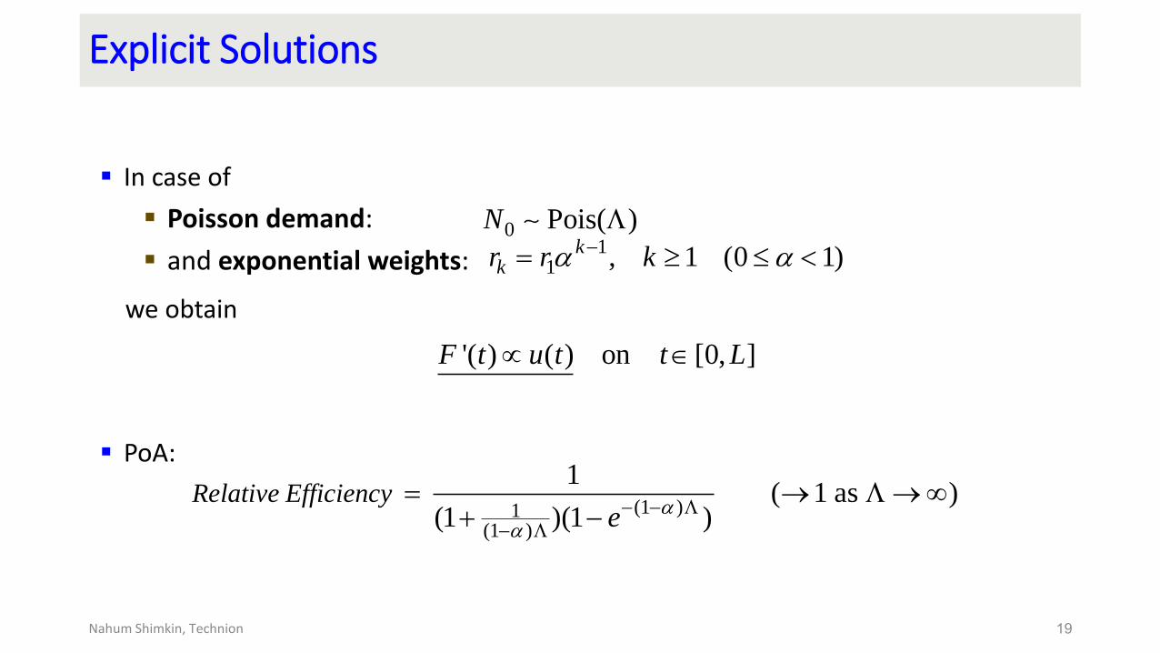
Explicit Solutions
In case of
Poisson demand:
and exponential weights:
we obtain
PoA:
19Nahum Shimkin, Technion
0 Pois( )N 1
1 , 1 (0 1)kkr r k
'( ) ( ) on [0, ]F t u t t L
(1 )1(1 )
1( 1 as )
(1 )(1 )Relative Efficiency
e
Nahum Shimkin, Technion20
When to Start a Trip:The Morning Commute Problem
The Bottleneck Model
Introduced by Vickrey (1969) to model the individual timing decisions of commuters who need to get to their destination at a certain time, during rush hours.
Also known as “the morning commute problem”.
Congestion is modeled as a FCFS fluid queue – assuming a single “bottleneck”.
Many generalizations in the transportation literature – we focus here the single queue, multiclass version.
21Nahum Shimkin, Technion
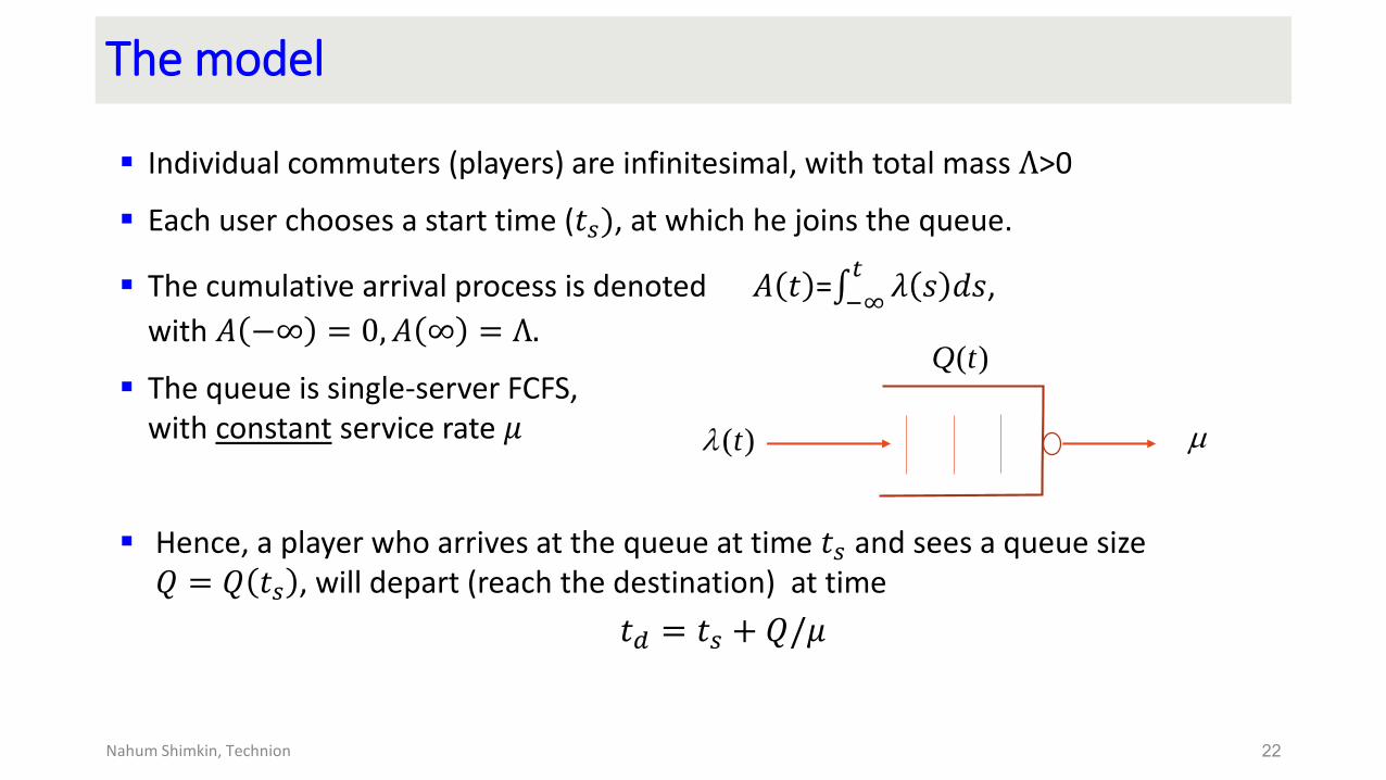
The model
Individual commuters (players) are infinitesimal, with total mass Λ>0
Each user chooses a start time (𝑡𝑠), at which he joins the queue.
The cumulative arrival process is denoted 𝐴 𝑡 = −∞𝑡𝜆 𝑠 𝑑𝑠,
with 𝐴 −∞ = 0, 𝐴 ∞ = Λ.
The queue is single-server FCFS, with constant service rate 𝜇
Hence, a player who arrives at the queue at time 𝑡𝑠 and sees a queue size𝑄 = 𝑄 𝑡𝑠 , will depart (reach the destination) at time
𝑡𝑑 = 𝑡𝑠 + 𝑄/𝜇
22Nahum Shimkin, Technion
( )t
( )Q t
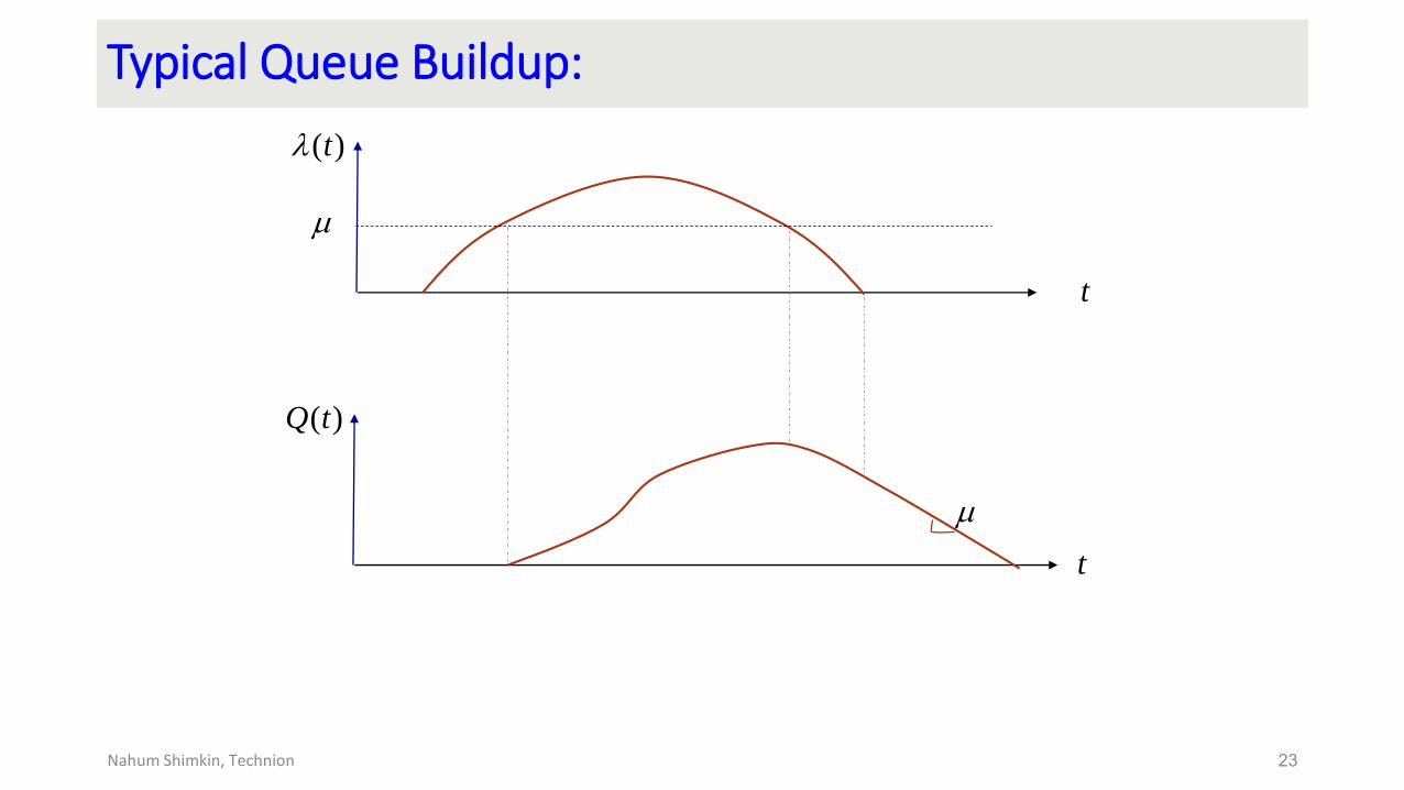
Typical Queue Buildup:
23Nahum Shimkin, Technion
t
( )Q t
t
( )t
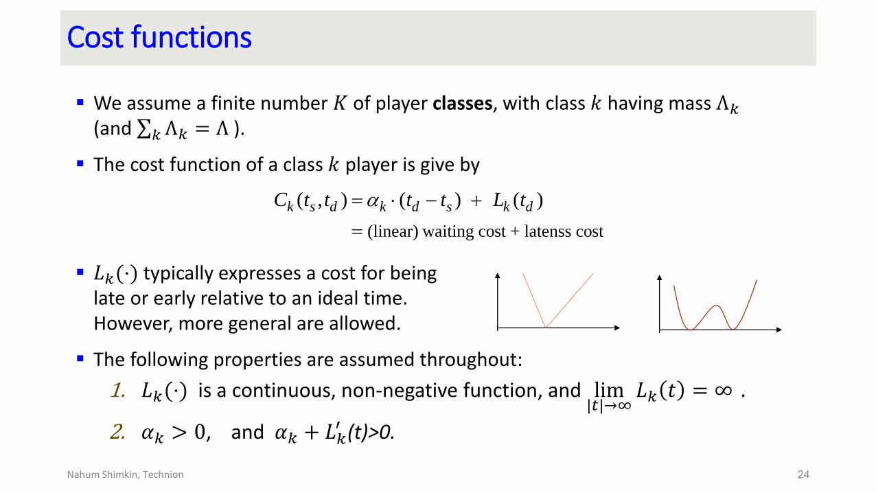
Cost functions
We assume a finite number 𝐾 of player classes, with class 𝑘 having mass Λ𝑘(and 𝑘 Λ𝑘 = Λ ).
The cost function of a class 𝑘 player is give by
𝐿𝑘(⋅) typically expresses a cost for being late or early relative to an ideal time. However, more general are allowed.
The following properties are assumed throughout:
1. 𝐿𝑘(⋅) is a continuous, non-negative function, and lim|𝑡|→∞𝐿𝑘 𝑡 = ∞ .
2. 𝛼𝑘 > 0, and 𝛼𝑘 + 𝐿𝑘′ (t)>0.
24Nahum Shimkin, Technion
(linear) waiting cost + latenss cost
( , ) ( ) ( )k s d k d s k dC t t t t L t
Equilibrium
A (Nash-Wardrop) equilibrium is defined, as usual, by the requirement that no player has an incentive to deviate. More concretely:
A arrival profile is a set of arrival densities {𝜆𝑘 𝑡 }𝑘∈𝐾, with −∞∞𝜆𝑘 𝑠 𝑑𝑠 = Λ𝑘 .
Given an arrival profile, each potential arrival at a time 𝑡𝑠 has a unique departure time 𝑡𝑑 𝑡𝑠 .
An arrival profile is a NEP if (essentially), for every class 𝑘,
In particular, the cost for all players of a given class is the same.
25Nahum Shimkin, Technion
*
( , )( ) 0 ( , ( )) min ( , ( ))
s
k k d k s d s kt
t C t t t C t t t c
Departure-time characterization
The NEP is naturally defined in terms of the decision variable 𝑡𝑠.
However, a more convenient representation is obtain by working with the departure times 𝑡𝑑. We follow the elegant formulation in Lindsey (2004).
26Nahum Shimkin, Technion
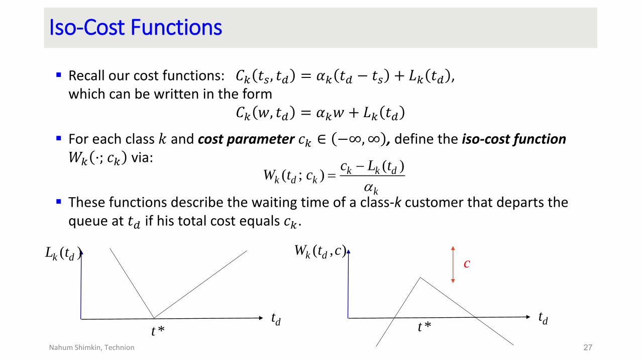
Iso-Cost Functions
Recall our cost functions: 𝐶𝑘 𝑡𝑠, 𝑡𝑑 = 𝛼𝑘 𝑡𝑑 − 𝑡𝑠 + 𝐿𝑘 𝑡𝑑 ,which can be written in the form
𝐶𝑘 𝑤, 𝑡𝑑 = 𝛼𝑘𝑤 + 𝐿𝑘 𝑡𝑑
For each class 𝑘 and cost parameter 𝑐𝑘 ∈ −∞,∞ , define the iso-cost function 𝑊𝑘 ⋅; 𝑐𝑘 via:
These functions describe the waiting time of a class-k customer that departs the queue at 𝑡𝑑 if his total cost equals 𝑐𝑘.
27Nahum Shimkin, Technion
( )( ; ) k k d
k d kk
c L tW t c
dt
( )k dL t
*tdt
( , )k dW t c
*t
c
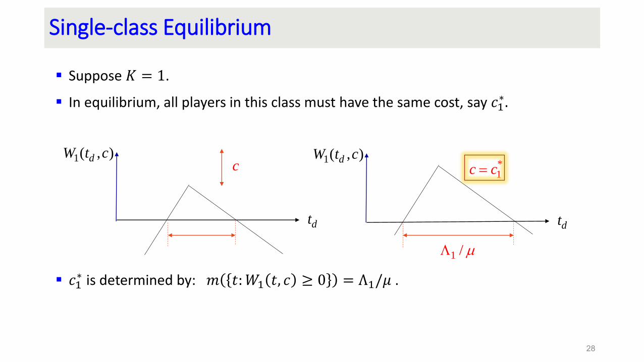
Single-class Equilibrium
Suppose 𝐾 = 1.
In equilibrium, all players in this class must have the same cost, say 𝑐1∗.
𝑐1∗ is determined by: 𝑚 𝑡:𝑊1 𝑡, 𝑐 ≥ 0 = Λ1/𝜇 .
28
dt
1( , )dW t cc
1 /
dt
1( , )dW t c*1c c
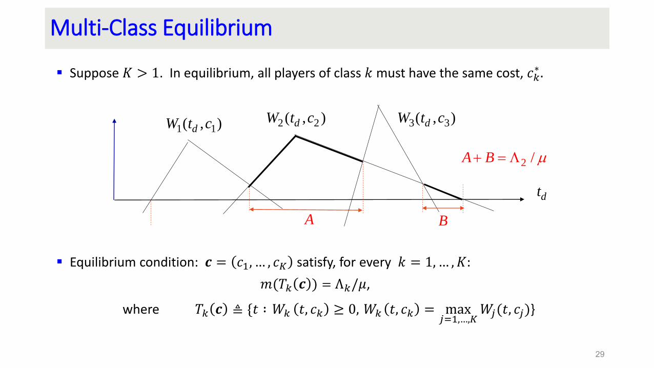
Multi-Class Equilibrium
Suppose 𝐾 > 1. In equilibrium, all players of class 𝑘 must have the same cost, 𝑐𝑘∗ .
Equilibrium condition: 𝒄 = 𝑐1, … , 𝑐𝐾 satisfy, for every 𝑘 = 1,… , 𝐾:
𝑚(𝑇𝑘 𝒄 ) = Λ𝑘/𝜇,
where 𝑇𝑘 𝒄 ≜ {𝑡 ∶ 𝑊𝑘 𝑡, 𝑐𝑘 ≥ 0, 𝑊𝑘 𝑡, 𝑐𝑘 = max𝑗=1,…,𝐾
𝑊𝑗(𝑡, 𝑐𝑗)}
29
2 /A B
dt
1 1( , )dW t c 2 2( , )dW t c 3 3( , )dW t c
A B
Multi-Class Equilibrium
Non-overlap Assumption: Assume (for now) that for any constants 𝑐1, … , 𝑐𝐾 and 𝑘 ≠ 𝑗, the following sets have measure zero:
{𝑡: 𝐿𝑘 𝑡, 𝑐𝑘 = 0}, {𝑡: 𝐿𝑘 𝑡, 𝑐𝑘 = 𝐿𝑗(𝑡, 𝑐𝑗)}
Proposition: An arrival profile 𝜆𝑘 𝑡 is a NEP if and only if there exists cost parameters 𝒄 = 𝑐1, … , 𝑐𝐾 that satisfy the above equilibrium condition, namely
𝑚 𝑇𝑘 𝒄 = Λ𝑘/𝜇, 𝑘 = 1,… , 𝐾 (#)
30Nahum Shimkin, Technion
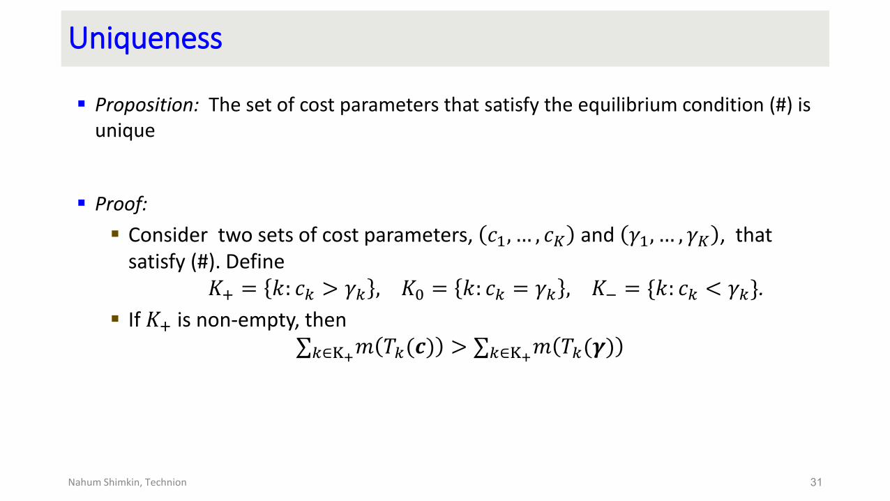
Uniqueness
Proposition: The set of cost parameters that satisfy the equilibrium condition (#) is unique
Proof:
Consider two sets of cost parameters, 𝑐1, … , 𝑐𝐾 and 𝛾1, … , 𝛾𝐾 , that satisfy (#). Define
𝐾+ = 𝑘: 𝑐𝑘 > 𝛾𝑘 , 𝐾0 = 𝑘: 𝑐𝑘 = 𝛾𝑘 , 𝐾− = {𝑘: 𝑐𝑘 < 𝛾𝑘}.
If 𝐾+ is non-empty, then 𝑘∈K+𝑚 𝑇𝑘(𝒄) > 𝑘∈K+𝑚 𝑇𝑘(𝜸)
31Nahum Shimkin, Technion
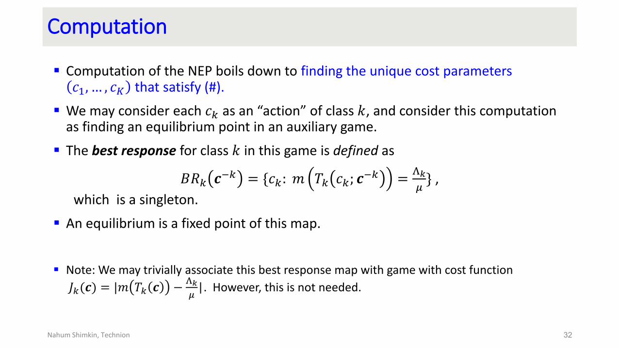
Computation
Computation of the NEP boils down to finding the unique cost parameters 𝑐1, … , 𝑐𝐾 that satisfy (#).
We may consider each 𝑐𝑘 as an “action” of class 𝑘, and consider this computation as finding an equilibrium point in an auxiliary game.
The best response for class 𝑘 in this game is defined as
𝐵𝑅𝑘 𝒄−𝑘 = {𝑐𝑘: 𝑚 𝑇𝑘 𝑐𝑘; 𝒄
−𝑘 =Λ𝑘
𝜇} ,
which is a singleton.
An equilibrium is a fixed point of this map.
Note: We may trivially associate this best response map with game with cost function
𝐽𝑘(𝒄) = |𝑚 𝑇𝑘 𝒄 −Λ𝑘
𝜇|. However, this is not needed.
32Nahum Shimkin, Technion
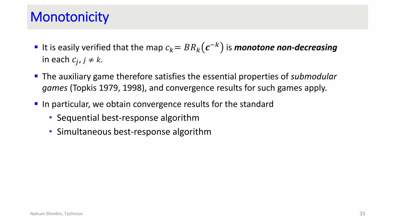
Monotonicity
It is easily verified that the map 𝑐𝑘= 𝐵𝑅𝑘 𝒄−𝑘 is monotone non-decreasing
in each 𝑐𝑗 , 𝑗 ≠ 𝑘.
The auxiliary game therefore satisfies the essential properties of submodular games (Topkis 1979, 1998), and convergence results for such games apply.
In particular, we obtain convergence results for the standard
• Sequential best-response algorithm
• Simultaneous best-response algorithm
33Nahum Shimkin, Technion
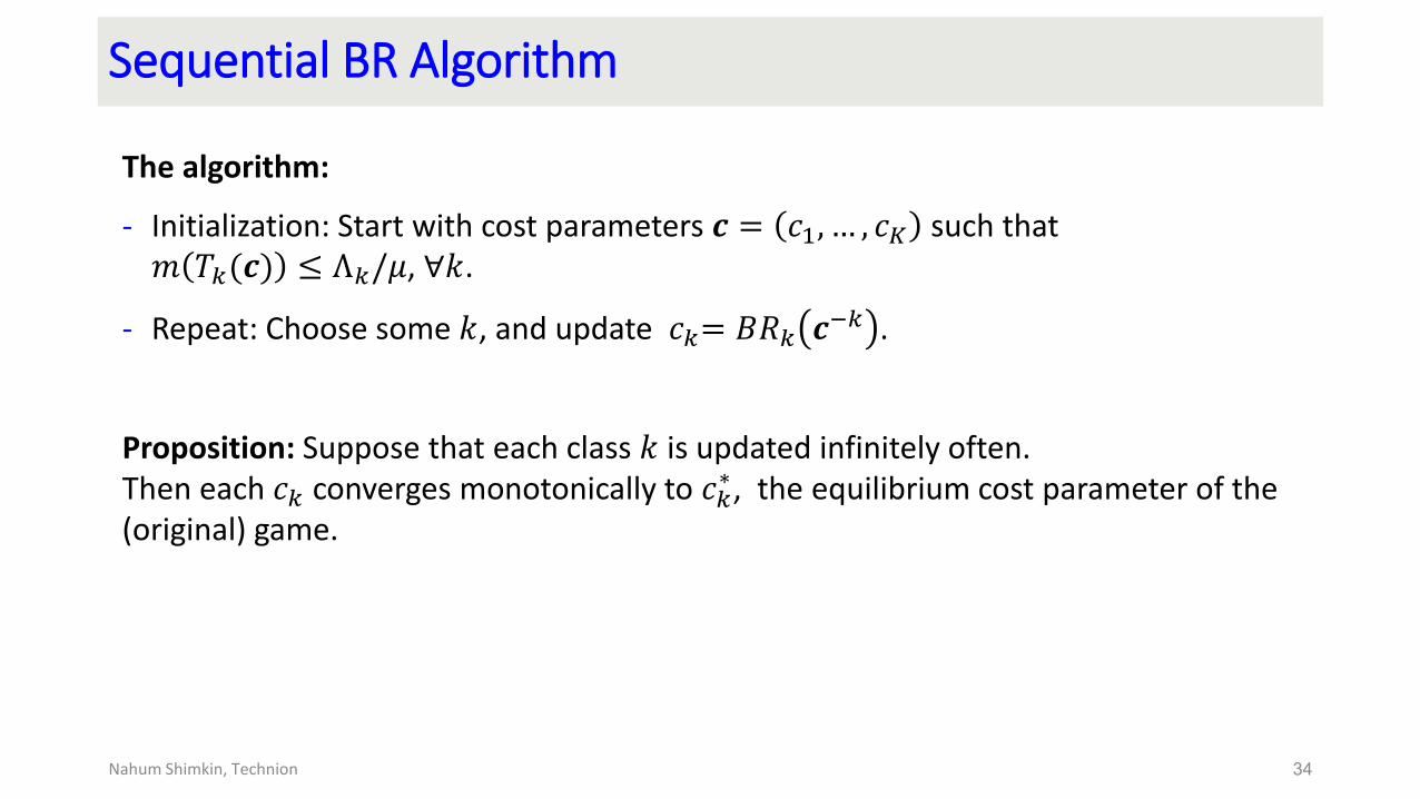
Sequential BR Algorithm
The algorithm:
- Initialization: Start with cost parameters 𝒄 = 𝑐1, … , 𝑐𝐾 such that 𝑚 𝑇𝑘(𝒄) ≤ Λ𝑘/𝜇, ∀𝑘.
- Repeat: Choose some 𝑘, and update 𝑐𝑘= 𝐵𝑅𝑘 𝒄−𝑘 .
Proposition: Suppose that each class 𝑘 is updated infinitely often. Then each 𝑐𝑘 converges monotonically to 𝑐𝑘
∗, the equilibrium cost parameter of the (original) game.
34Nahum Shimkin, Technion
Sequential BR Algorithm
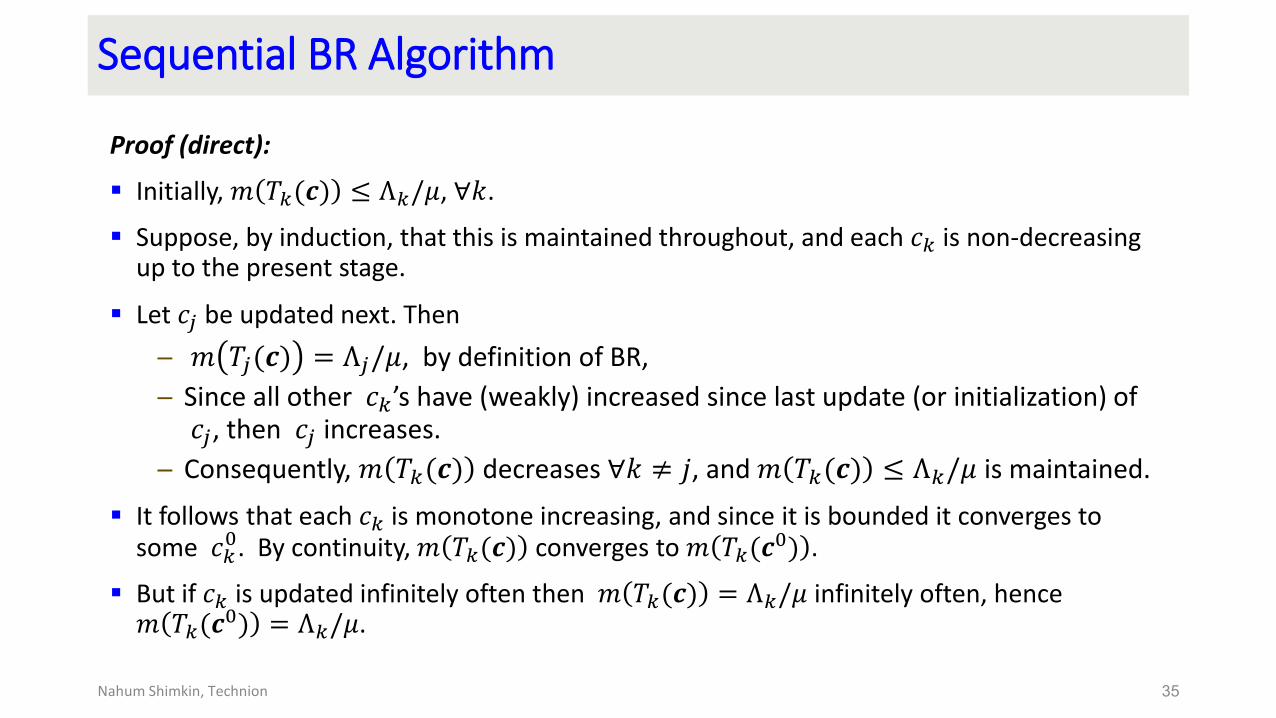
Proof (direct):
Initially, 𝑚 𝑇𝑘(𝒄) ≤ Λ𝑘/𝜇, ∀𝑘.
Suppose, by induction, that this is maintained throughout, and each 𝑐𝑘 is non-decreasing up to the present stage.
Let 𝑐𝑗 be updated next. Then
─ 𝑚 𝑇𝑗(𝒄) = Λ𝑗/𝜇, by definition of BR,
─ Since all other 𝑐𝑘’s have (weakly) increased since last update (or initialization) of 𝑐𝑗, then 𝑐𝑗 increases.
─ Consequently, 𝑚 𝑇𝑘(𝒄) decreases ∀𝑘 ≠ 𝑗, and 𝑚 𝑇𝑘(𝒄) ≤ Λ𝑘/𝜇 is maintained.
It follows that each 𝑐𝑘 is monotone increasing, and since it is bounded it converges to some 𝑐𝑘
0. By continuity, 𝑚 𝑇𝑘(𝒄) converges to 𝑚 𝑇𝑘(𝒄0) .
But if 𝑐𝑘 is updated infinitely often then 𝑚 𝑇𝑘(𝒄) = Λ𝑘/𝜇 infinitely often, hence 𝑚 𝑇𝑘(𝒄
0) = Λ𝑘/𝜇.
35Nahum Shimkin, Technion
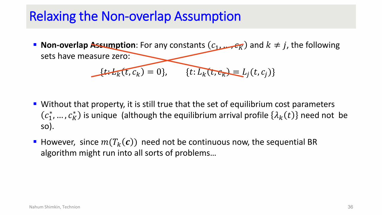
Relaxing the Non-overlap Assumption
Non-overlap Assumption: For any constants 𝑐1, … , 𝑐𝐾 and 𝑘 ≠ 𝑗, the following sets have measure zero:
{𝑡: 𝐿𝑘 𝑡, 𝑐𝑘 = 0}, {𝑡: 𝐿𝑘 𝑡, 𝑐𝑘 = 𝐿𝑗(𝑡, 𝑐𝑗)}
Without that property, it is still true that the set of equilibrium cost parameters 𝑐1∗, … , 𝑐𝐾
∗ is unique (although the equilibrium arrival profile 𝜆𝑘 𝑡 need not be so).
However, since 𝑚(𝑇𝑘 𝒄 ) need not be continuous now, the sequential BR algorithm might run into all sorts of problems…
36Nahum Shimkin, Technion
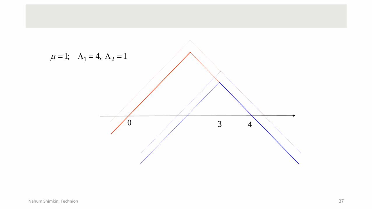
37Nahum Shimkin, Technion
1 21; 4, 1
40 3
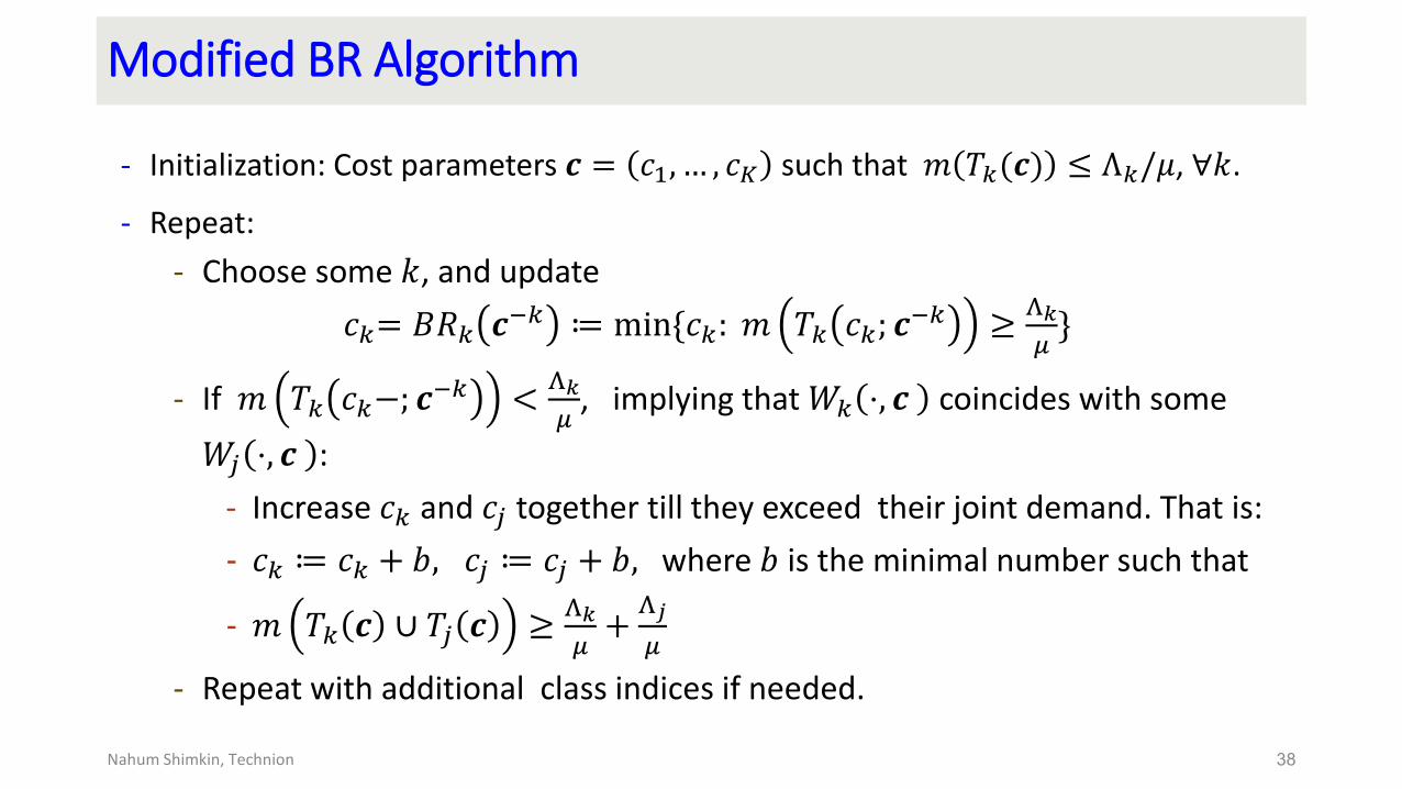
Modified BR Algorithm
- Initialization: Cost parameters 𝒄 = 𝑐1, … , 𝑐𝐾 such that 𝑚 𝑇𝑘(𝒄) ≤ Λ𝑘/𝜇, ∀𝑘.
- Repeat:
- Choose some 𝑘, and update
𝑐𝑘= 𝐵𝑅𝑘 𝒄−𝑘 ≔ min{𝑐𝑘: 𝑚 𝑇𝑘 𝑐𝑘; 𝒄
−𝑘 ≥Λ𝑘
𝜇}
- If 𝑚 𝑇𝑘 𝑐𝑘−; 𝒄−𝑘 <
Λ𝑘
𝜇, implying that 𝑊𝑘 ⋅, 𝒄 coincides with some
𝑊𝑗 ⋅, 𝒄 :
- Increase 𝑐𝑘 and 𝑐𝑗 together till they exceed their joint demand. That is:
- 𝑐𝑘 ≔ 𝑐𝑘 + 𝑏, 𝑐𝑗 ≔ 𝑐𝑗 + 𝑏, where 𝑏 is the minimal number such that
- 𝑚 𝑇𝑘 𝒄 ∪ 𝑇𝑗 𝒄 ≥Λ𝑘
𝜇+Λ𝑗
𝜇
- Repeat with additional class indices if needed.
38Nahum Shimkin, Technion
Additional Issues
Stopping criteria
Convergence rates
(Network Problems)
39Nahum Shimkin, Technion

Nahum Shimkin, Technion 40
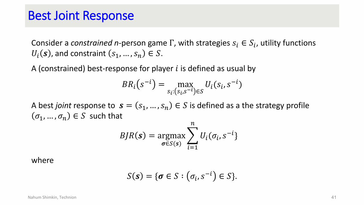
Best Joint Response
Consider a constrained n-person game Γ, with strategies 𝑠𝑖 ∈ 𝑆𝑖, utility functions 𝑈𝑖 𝒔 , and constraint 𝑠1, … , 𝑠𝑛 ∈ 𝑆.
A (constrained) best-response for player 𝑖 is defined as usual by
𝐵𝑅𝑖 𝑠−𝑖 = max
𝑠𝑖: 𝑠𝑖,𝑠−𝑖 ∈𝑆𝑈𝑖(𝑠𝑖 , 𝑠
−𝑖)
A best joint response to 𝒔 = 𝑠1, … , 𝑠𝑛 ∈ 𝑆 is defined as a the strategy profile 𝜎1, … , 𝜎𝑛 ∈ 𝑆 such that
𝐵𝐽𝑅 𝒔 = argmax𝝈∈𝑆(𝒔)
𝑖=1
𝑛
𝑈𝑖(𝜎𝑖 , 𝑠−𝑖}
where
𝑆 𝒔 = {𝝈 ∈ 𝑆 ∶ 𝜎𝑖 , 𝑠−𝑖 ∈ 𝑆}.
41Nahum Shimkin, Technion
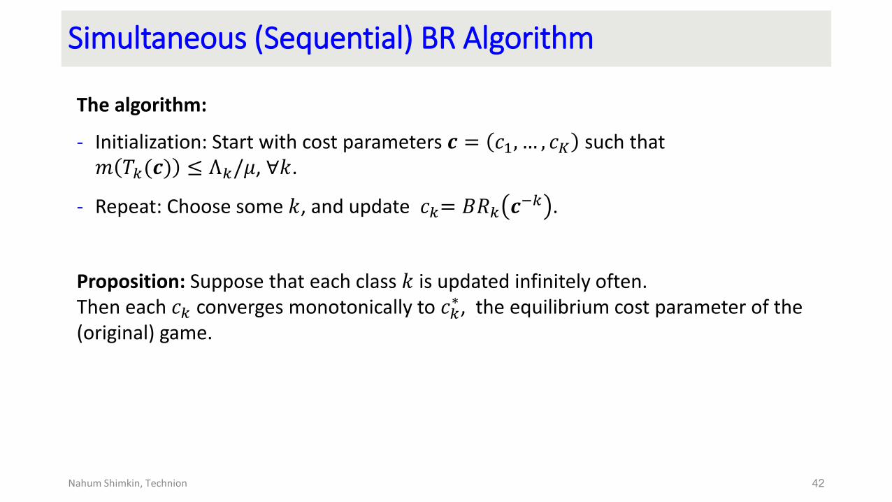
Simultaneous (Sequential) BR Algorithm
The algorithm:
- Initialization: Start with cost parameters 𝒄 = 𝑐1, … , 𝑐𝐾 such that 𝑚 𝑇𝑘(𝒄) ≤ Λ𝑘/𝜇, ∀𝑘.
- Repeat: Choose some 𝑘, and update 𝑐𝑘= 𝐵𝑅𝑘 𝒄−𝑘 .
Proposition: Suppose that each class 𝑘 is updated infinitely often. Then each 𝑐𝑘 converges monotonically to 𝑐𝑘
∗, the equilibrium cost parameter of the (original) game.
42Nahum Shimkin, Technion