Embed Size (px)
Citation preview

Strategic Production Planning
Now showing at your local university

Production planning is the activity of establishing production goals over a future time period calledthe planning horizon. The objective is to plan theoptimal use of resources to meet stated productionrequirements.
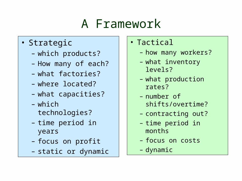
A Framework
• Strategic– which products?
– How many of each?
– what factories?
– where located?
– what capacities?
– which technologies?
– time period in years
– focus on profit
– static or dynamic
• Tactical– how many workers?
– what inventory levels?
– what production rates?
– number of shifts/overtime?
– contracting out?
– time period in months
– focus on costs
– dynamic
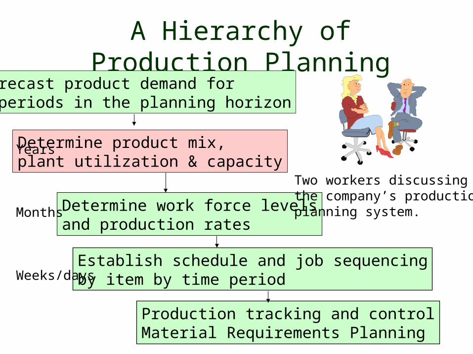
A Hierarchy of Production PlanningForecast product demand for t periods in the planning horizon
Determine product mix,plant utilization & capacity
Determine work force levelsand production rates
Establish schedule and job sequencingby item by time period
Production tracking and controlMaterial Requirements Planning
Two workers discussingthe company’s productionplanning system.
Years
Months
Weeks/days

Three Levels of Planning
• Strategic– Everything subject to change
• Tactical– Infrastructure (e.g. factories, warehouses, products)
remains fixed– Resources (e.g. machinery, raw material, labor) may
change
• Operational– Infrastructure and resources are fixed– Basic question is how best to utilize them

Aggregate Planning
• Macro production planning• Products lumped together to form an aggregate
product• Aggregated products and capacity expressed in
terms of an average item if similar• If items are different, then money, production
hours, or weight (e.g. tons of steel) may be used• Translate demand forecasts into a blueprint for
planning staff and production levels• Can be applied to strategic or tactical planning

Spreadsheet Methods
• Zero inventory strategy– produce to meet monthly demand– no inventories– work force fluctuates
• Level production strategy– maintain constant production rate– inventory fluctuates– constant work force

Production Strategies
time
cumulativenumberof units constant production rate
demand curve
variable production rate
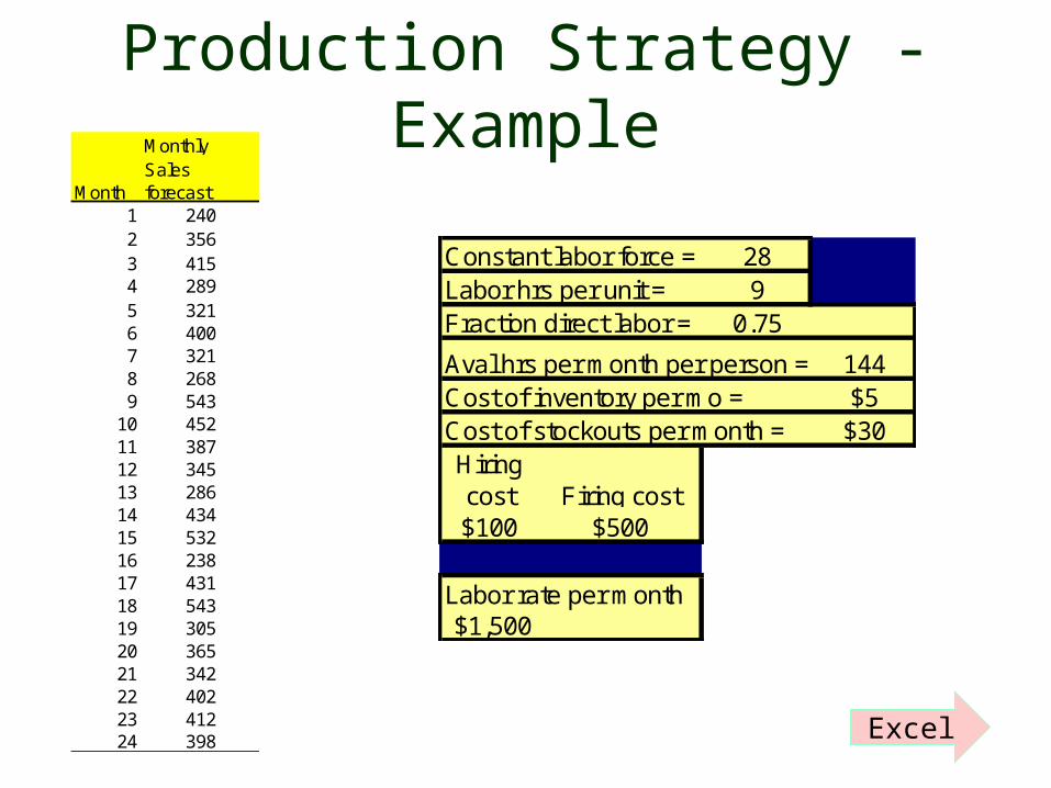
Production Strategy - Example
Constant labor force = 28Labor hrs per unit = 9Fraction direct labor = 0.75
Aval hrs per month per person = 144Cost of inventory per mo = $5Cost of stockouts per month = $30Hiring cost Firing cost$100 $500
Labor rate per month$1,500
Monthly
MonthSales forecast
1 2402 3563 4154 2895 3216 4007 3218 2689 543
10 45211 38712 34513 28614 43415 53216 23817 43118 54319 30520 36521 34222 40223 41224 398 Excel
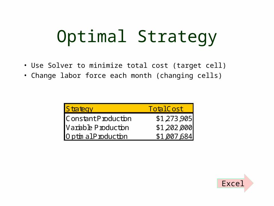
Optimal Strategy
• Use Solver to minimize total cost (target cell)
• Change labor force each month (changing cells)
Strategy Total CostConstant Production $1,273,905Variable Production $1,202,000Optimal Production $1,007,684
Excel

A Static Strategic Planning ModelAssumptions
• deterministic– all input parameters are known
• selling price is fixed
• unit cost does not vary with production levels (no learning curve effect)
• demand is over a fixed planning horizon (static)
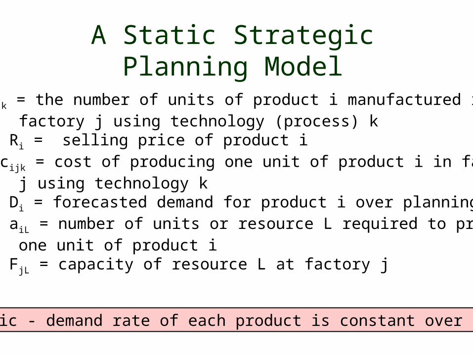
A Static Strategic Planning Model
Let xijk = the number of units of product i manufactured in factory j using technology (process) k
Ri = selling price of product i cijk = cost of producing one unit of product i in factory
j using technology k Di = forecasted demand for product i over planning horizon aiL = number of units or resource L required to produce
one unit of product i FjL = capacity of resource L at factory j
Static - demand rate of each product is constant over time.
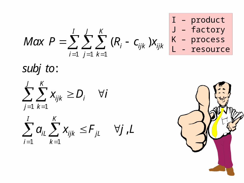
Max P R c x
subj to
x D i
a x F j L
i ijk ijkk
K
j
J
i
I
ijkk
K
ij
J
iLi
I
ijkk
K
jL
( )
:
,
111
11
1 1
I – productJ – factoryK – processL - resource
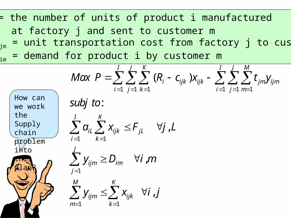
Let yijm = the number of units of product i manufactured at factory j and sent to customer m
tjm = unit transportation cost from factory j to customer m Dim = demand for product i by customer m
Max P R c x t y
subj to
a x F j L
y D i m
y x i j
i ijk ijkk
K
j
J
i
I
jm ijmm
M
j
J
i
I
iLi
I
ijkk
K
jL
ijmj
J
im
ijmm
M
ijkk
K
( )
:
,
,
,
111 111
1 1
1
1 1
How can we work theSupply chain problem intothis plan?
This model is becomingquite interesting. How can I throw a fixed startupcost into this?
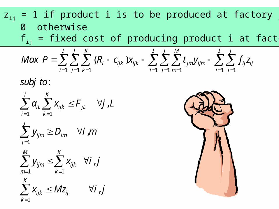
Let zij = 1 if product i is to be produced at factory j; 0 otherwise
fij = fixed cost of producing product i at factory j
Max P R c x t y f z
subj to
a x F j L
y D i m
y x i j
x Mz i j
i ijk ijkk
K
j
J
i
I
jm ijmm
M
j
J
i
I
ij ijj
J
i
I
iLi
I
ijkk
K
jL
ijmj
J
im
ijmm
M
ijkk
K
ijkk
K
ij
( )
:
,
,
,
,
111 111 11
1 1
1
1 1
1

The Breakeven Point - Bij
1 1
0K K
ijk ijk ijk k
If x then x B
Isn’t there some
way we can account for the
break-even point?
1
1
K
ijk ij ijk
K
ijk ijk
x B z
x Mz
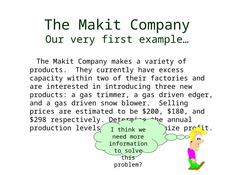
The Makit CompanyOur very first example…
The Makit Company makes a variety of products. They currently have excess capacity within two of their factories and are interested in introducing three new products: a gas trimmer, a gas driven edger, and a gas driven snow blower. Selling prices are estimated to be $200, $180, and $298 respectively. Determine the annual production levels that will maximize profit.
I think we need more information
to solve this problem?

Makit CompanyProduct Prod
1Prod 1 Prod
2Prod 2 Prod 3 Prod 3 Prod 3
Factory location
Dayton Tijuana Dayton Tijuana Dayton Dayton Tijuana
Per unit data Process A
Process B
Production cost
$25 20 18 12 36 30 32
Material cost $40 30 24 24 18 18 16
Labor hr 12 12 23 23 18 6 18
Machine hr 2 2 6 6 5 11 5
Fixed setup cost
10000 15000 5000 6000 1000 120000 8000
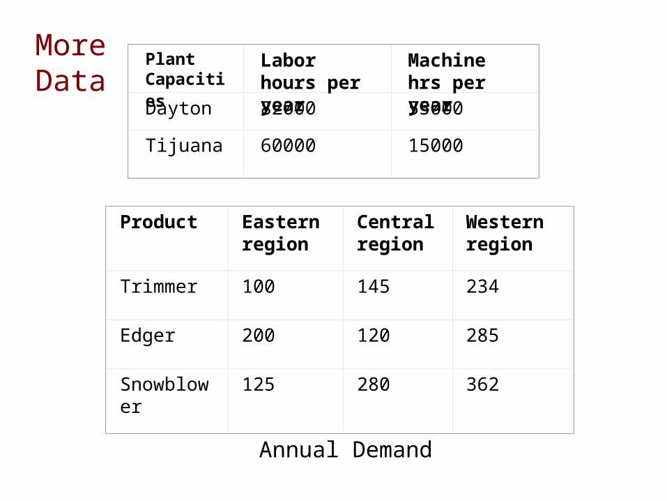
PlantCapacities
Labor hours per year
Machine hrs per year
Dayton 82000 55000
Tijuana 60000 15000
Product Eastern region
Central region
Western region
Trimmer 100 145 234
Edger 200 120 285
Snowblower 125 280 362
MoreData
Annual Demand

Plant Eastern region
Central region
Western region
Dayton 5 8 10
Tijuana, Mexico
12 7 6
Distribution Costs$ per unit

Xijk = number of units of product i produced at plant j using process k
Yijl = number of units of product i produced at plant j and sent to region l
Zij = fixed cost of producing product i at plant j
MAX Profit:
z = - 10000 Z11 - 15000 Z12 - 5000 Z21 - 6000 Z22 - 1000 Z311 - 12000 Z312 - 8000 Z32 + 135 X11 + 150 X12 + 138 X21 + 144 X22 + 244 X311 + 250 X312 + 250 X32 -5 Y111 - 8 Y112 - 10 Y113 - 12 Y121 - 7 Y122 - 6 Y123 -5 Y211 - 8 Y212 - 10 Y213 - 12 Y221 - 7 Y222-6 Y223 - 5 Y311 - 8 Y312 - 10 Y313 - 12 Y321 - 7 Y322 - 6 Y323
The Formulation

SUBJECT TORegional demands: 2) Y111 + Y121 = 100 3) Y211 + Y221 = 200 4) Y311 + Y321 = 125 5) Y112 + Y122 = 145 6) Y212 + Y222 = 120 7) Y312 + Y322 = 280 8) Y113 + Y123 = 234 9) Y213 + Y223 = 285 10) Y313 + Y323 = 362Plant capacities: 11) 12 X11 + 23 X21 + 18 X311 + 6 X312 <= 82000 12) 12 X12 + 23 X22 + 18 X32 <= 60000 13) 2 X11 + 6 X21 + 5 X311 + 11 X312 <= 55000 14) 2 X12 + 6 X22 + 5 X32 <= 15000
Eastern
Central
Western

Fixed costs: 15) - 10000 Z11 + X11 <= 0 16) - 10000 Z21 + X21 <= 0 17) - 10000 Z311 + X311 <= 0 18) - 10000 Z312 + X312 <= 0 19) - 10000 Z12 + X12 <= 0 20) - 10000 Z22 + X22 <= 0 21) - 10000 Z32 + X32 <= 0
Production – Distribution dependency: 22) - X11 + Y111 + Y112 + Y113 = 0 23) - X21 + Y211 + Y212 + Y213 = 0 24) - X311 - X312 + Y311 + Y312 + Y313 = 0 25) - X12 + Y121 + Y122 + Y123 = 0 26) - X22 + Y221 + Y222 + Y223 = 0 27) - X32 + Y321 + Y322 + Y323 = 0 ENDINT Z11 Z12 Z21 Z22 Z311 Z312 Z32

Product Prod 1
Prod 1
Prod 2
Prod 2
Prod 3 Prod 3 Prod 3
Factory location
Dayton
Tijuana
Dayton
Tijuana
Dayton Dayton Tijuana
Process A
Process B
Units produced
479 605 767
Distribution
Eastern region
100 200 125
Central region
145 120 280
Western region
234 285 362
The Solution – Max Profit = $309,064

A “Solver” Solution
Let me show you what solver can do with this problem.

Another Example?
Could you share with us another
example?
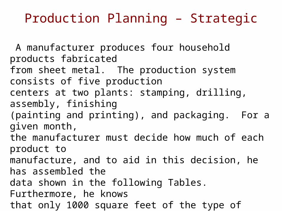
Production Planning – Strategic
A manufacturer produces four household products fabricated from sheet metal. The production system consists of five production centers at two plants: stamping, drilling, assembly, finishing (painting and printing), and packaging. For a given month, the manufacturer must decide how much of each product to manufacture, and to aid in this decision, he has assembled the data shown in the following Tables. Furthermore, he knows that only 1000 square feet of the type of sheet metal used for products 2 and 4 will be available at each plant during the month. Product 2 requires 2.0 square feet per unit and product 4 uses 1.2 square feet per unit.

TABLE 1 Production Data
PRODUCTION RATES IN HOURS PER UNIT
production
Department prod 1 prod 2 prod 3 prod 4 hours available Plant 1 Plant 2
Stamping 0.03 0.15 0.05 0.10 150 250Drilling 0.06 0.12 - 0.10 200 200Assembly 0.05 0.10 0.05 0.12 300 200Finishing 0.04 0.20 0.03 0.12 175 275Packaging 0.02 0.06 0.02 0.05 300 100

TABLE 2 Product Data
NET SELLING VARIABLE SALES POTENTIALProduct PRICE/UNIT COST/UNIT MINIMUM MAXIMUM
Plant 1 Plant 2
1 10 $6 5 1000 60002 25 $15 13 - 5003 16 $11 10 500 30004 20 $14 12 100 1000

TABLE 3 distribution costs
Plant /warehouse Warehouse 1 Warehouse 2Plant 1 $2 1Plant 2 3 4
Demands – as a percent of 40 % 60 %above sales potential

FormulationVariable definitions:
Xij = number of units of product i produced at plant jYijk = number of units of product i shipped from
plant j to warehouse k Profit = selling price
– variable cost – distribution costs MAX 4 X11 + 5 X12 + 10 X21 + 12 X22 + 5 X31 + 6 X32 + 6 X41 + 8 X42 - 2 Y111 - 2 Y211 - 2 Y311 - 2 Y411 - Y112 - Y212 - Y312 - Y412 - 3 Y121 - 3 Y221 - 3 Y321 - 3 Y421 - 4 Y122 - 4 Y222 - 4 Y322 - 4 Y422

Constraints
Department processing constraints
2) 0.03 X11 + 0.15 X21 + 0.05 X31 + 0.1 X41 <= 1503) 0.06 X11 + 0.12 X21 + 0.1 X41 <= 2004) 0.05 X11 + 0.1 X21 + 0.05 X31 + 0.12 X41 <= 3005) 0.04 X11 + 0.2 X21 + 0.03 X31 + 0.12 X41 <= 1756) 0.02 X11 + 0.06 X21 + 0.02 X31 + 0.05 X41 <= 300
7) 0.03 X12 + 0.15 X22 + 0.05 X32 + 0.1 X42 <= 2508) 0.06 X12 + 0.12 X22 + 0.1 X42 <= 2009) 0.05 X12 + 0.1 X22 + 0.05 X32 + 0.12 X42 <= 20010) 0.04 X12 + 0.2 X22 + 0.03 X32 + 0.12 X42 <= 27511) 0.02 X12 + 0.06 X22 + 0.02 X32 + 0.05 X42 <= 100
Plant 1
Plant 2
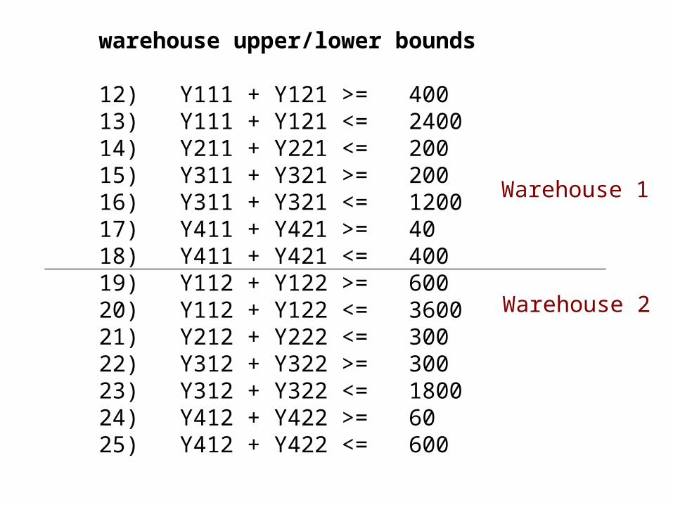
warehouse upper/lower bounds
12) Y111 + Y121 >= 40013) Y111 + Y121 <= 240014) Y211 + Y221 <= 20015) Y311 + Y321 >= 20016) Y311 + Y321 <= 120017) Y411 + Y421 >= 4018) Y411 + Y421 <= 40019) Y112 + Y122 >= 60020) Y112 + Y122 <= 360021) Y212 + Y222 <= 30022) Y312 + Y322 >= 30023) Y312 + Y322 <= 180024) Y412 + Y422 >= 6025) Y412 + Y422 <= 600
Warehouse 1
Warehouse 2

produce only what is to be shipped26) - X11 + Y111 + Y112 = 027) - X21 + Y211 + Y212 = 028) - X31 + Y311 + Y312 = 029) - X41 + Y411 + Y412 = 0 30) - X12 + Y121 + Y122 = 031) - X22 + Y221 + Y222 = 032) - X32 + Y321 + Y322 = 033) - X42 + Y421 + Y422 = 0
sheet metal constraint• 2 X21 + 1.2 X41 <= 1000 • 2 X22 + 1.2 X42 <= 1000

SolutionProd 1 Prod 2 Prod 3 Prod 4
Plant 1 2 1 2 1 2 1 2
3333.3 1680 440 1000 1200 100
Warehouse1 1680 200 1200 40
2 3333.3 240 1000 60
max profit = $25,120

Alternate Solution
Prod 1 Prod 2 Prod 3 Prod 4Plant 1 2 1 2 1 2 1 2
3333.3 880 440 1000 2000 100
Warehouse1 880 200 1200 40
2 3333.3 240 1000 800 60
max profit = $25,120

Production Planning
The Dynamic Case
Look, we must consider the fact that demands are
going to fluctuate significantly over the
next several years

Let xijt = number of units or product i produced by process j in period t
sit = number of units of product i sold in period t
Iit = number of units of product i in inventory at the end of period t
Decision Variables

Model Parameters
rit = revenue from selling one unit of product i in period tcijt = variable production cost of one unit of product i by process j in period tFit = maximum sales forecasted for product i in period taijk = units of resource k required for each unit of product i
produced by process j.bkt = number of units of resource k available in time
period tdit = inventory carrying cost for product i during period thijt = cost of changing production levels for product i
using process j in period t
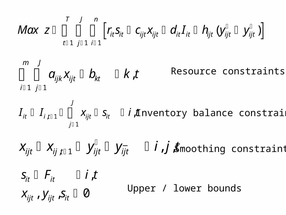
Max z r s c x d I h y yit it ijt ijt it it ijt ijt ijti
n
j
J
t
T
( )
111
a x b k tijk ijt ktj
J
i
m
11
, Resource constraints
I I x s i tit i t ijt itj
J
, ,1
1
Inventory balance constraints
x x y y i j tijt ij t ijt ijt
,_ , ,1 Smoothing constraints
s F i t
x y sit it
ijt ijt it
,
, , 0 Upper / lower bounds

Turn-in Problem #3
This is a great exercisefor the student!
Due Monday September 28Web Submission