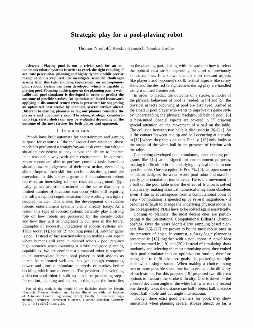
Strategic play for a pool-playing robot

Thomas Nierhoff, Kerstin Heunisch, Sandra Hirche

Abstract— Playing pool is not a trivial task for an au-tonomous robotic system: In order to excel, the tight coupling ofaccurate perception, planning and highly dynamic while precisemanipulation is required. To investigate scientific challengesarising from this tight coupling requirement an anthropomor-phic robotic system has been developed, which is capable ofplaying pool. Focusing in this paper on the planning part, a well-calibrated pool simulator is developed in order to predict theoutcome of possible strokes. An optimization based frameworkapplying a discounted return term is presented for suggestingan optimized next stroke by planning several strokes ahead.Different to existing planners so far, our planner considers theplayer’s and opponent’s skill. Therefore, strategic considera-tions (e.g. safety shots) can now be evaluated depending on theoutcome of the next strokes for both player and opponent.

I. I NTRODUCTION

People have built automata for entertainment and gamingpurpose for centuries. Like the Jaquet-Droz automata, thosemachines performed a straightforward task execution withoutsituation assessment as they lacked the ability to interactin a reasonable way with their environment. In contrast,recent robots are able to perform complex tasks based onsituation-aware judgement of their next action, even beingable to improve their skill for specific tasks through multipleexecution. In this context, game and entertainment robotsrepresent an interesting robotics research playground. Typ-ically games are still structured in the sense that only alimited number of situations can occur while still requiringthe full perception-cognition-action loop working in a tightlycoupled manner. This makes the development of suitablerobotic entertainment systems viable already today. As aresult, this type of robotic systems certainly play a strongrole on how robots are perceived by the society todayand how they will be integrated in our lives in the future.Examples of successful integration of robotic systems are:Table soccer [1], soccer [2] and ping pong [3]. Another gameis pool. Instead of fast reactions/decision making - an aspectwhere humans still excel humanoid robots - pool requireshigh accuracy when executing a stroke and good planningcapabilities. We are confident a humanoid robot is superiorto an intermediate human pool player in both aspects asit can be calibrated well and has got enough computingpower and time to simulate hundreds of strokes beforedeciding which one to execute. The problem of developinga descent pool robot is split up into three processing steps:Perception, planning and action. In this paper the focus lies

Part of this work is the result of the Bachelor thesis by KerstinHeunisch. Thomas Nierhoff and Sandra Hirche are with the Instituteof Automatic Control Engineering (LSR), Faculty of Electrical Engi-neering, Technische Universitat Munchen, D-80290 Munchen, Germany{tn, hirche}@tum.de.

on the planning part, dealing with the question how to selectthe optimal next stroke depending on a set of previouslysimulated ones. It is shown that the most relevant aspectslike player’s and opponent’s skill, tactical aspects like safetyshots and the desired farsightedness during play are handledusing a unified frameword.

In order to predict the outcome of a stroke, a model ofthe physical behaviour of pool is needed. In [4] and [5], thephysical aspects occurring at pool are displayed. Aimed atthe amateur pool player who wants to improve his game styleby understanding the physical background behind pool, [6]is best-suited. Special aspects are covered in [7] drawingspecial attention on the movement of a ball on the table.The collision between two balls is discussed in [8]–[11]. Sois the contact between cue tip and ball occurring at a strokein [12] where they focus on spin. Finally, [13] only looks atthe stroke of the white ball in the presence of friction withthe table.

Concerning developed pool simulators, most existing pro-grams like [14] are designed for entertainment purposes,making it difficult to fit the underlying physical model to onespecific table. One exception is PoolFiz [4], an open sourcesimulator designed for a real-world pool robot and used foryearly pool simulation tournaments. Here, the movement ofa ball on the pool table under the effect of friction is solvedanalytically, making classical numerical integration obsolete.Even if this is advantageous from a computational point ofview - computation is speeded up by several magnitudes - itbecomes difficult to change the underlying physical model asthe corresponding PDEs have to be solved again analytically.

Coming to planners, the most decent ones are partici-pating at the International Computational Billiards Champi-onships. Over the years Monte-Carlo sampling based plan-ners like [15]–[17] are proven to be the most robust ones inthe presence of noise. In contrast, a fuzzy logic planner ispresented in [18] together with a pool robot. A novel ideais demonstrated in [19] and [20]: Instead of simulating shotsrandomly and selecting the most promising ones, they embedtheir pool simulator into an optimization routine, thereforebeing able to fulfil advanced goals like pocketing multipleballs with a single stroke. When making a choice amongtwo or more possible shots, one has to evaluate the difficultyof each stroke. For this purpose [19] proposed two differentoptions to measure the stroke difficulty: One is based on theallowed deviation angle of the white ball whereas the secondone directly takes the distance cue ball - object ball, distanceobject ball - hole and cut angle into account.

Though there exist good planners for pool, they showlimitations when planning several strokes ahead: So far, a

lot of important variables like the strength of the playerand opponent, tactical decisions or the far-sightedness duringposition play are considered just insufficiently.

The contribution of this paper is therefore a frameworktackling the planning problem for a robotic system whenplaying pool. It consists on the one hand of a physics-basedpool simulator with parameters identified through a real pooltable. On the other hand a sampling-based planning strategyis adopted, simulating the next most likely strokes for both,the robot and the opponent. By using a cost function based ona discounted return function, the outcome of several strokesahead is represented as a single scalar value. This results inan optimization problem over a search tree. Under certainassumptions, we show how a fast solution can be obtainedthrough dynamic programming. The key aspect of this paperis how an optimal next stroke is derived taking both theplayer’s and opponent’s skill as well as tactical aspects likesafety shots into consideration.

The remainder of this paper is organized as follows: Sec. IIprovides a brief overview over the existing anthropomorphicrobot used for pool. In Sec. III the underlying equationsfor the implemented pool simulator are constituted. Sec. IVdisplays how the simulator is fitted to a real table. Last,Sec. V concentrates on the question how an optimized nextstroke is suggested for the player.

II. POOL-PLAYING ROBOTIC SYSTEM

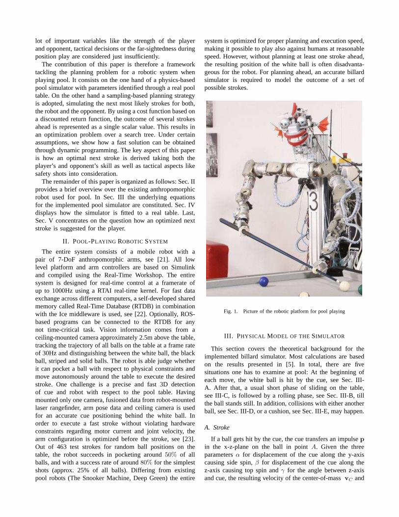
The entire system consists of a mobile robot with apair of 7-DoF anthropomorphic arms, see [21]. All lowlevel platform and arm controllers are based on Simulinkand compiled using the Real-Time Workshop. The entiresystem is designed for real-time control at a framerate ofup to 1000Hz using a RTAI real-time kernel. For fast dataexchange across different computers, a self-developed sharedmemory called Real-Time Database (RTDB) in combinationwith the Ice middleware is used, see [22]. Optionally, ROS-based programs can be connected to the RTDB for anynot time-critical task. Vision information comes from aceiling-mounted camera approximately 2.5m above the table,tracking the trajectory of all balls on the table at a frame rateof 30Hz and distinguishing between the white ball, the blackball, striped and solid balls. The robot is able judge whetherit can pocket a ball with respect to physical constraints andmove autonomously around the table to execute the desiredstroke. One challenge is a precise and fast 3D detectionof cue and robot with respect to the pool table. Havingmounted only one camera, fusioned data from robot-mountedlaser rangefinder, arm pose data and ceiling camera is usedfor an accurate cue positioning behind the white ball. Inorder to execute a fast stroke without violating hardwareconstraints regarding motor current and joint velocity, thearm configuration is optimized before the stroke, see [23].Out of 463 test strokes for random ball positions on thetable, the robot succeeds in pocketing around50% of allballs, and with a success rate of around80% for the simplestshots (approx. 25% of all balls). Differing from existingpool robots (The Snooker Machine, Deep Green) the entire

system is optimized for proper planning and execution speed,making it possible to play also against humans at reasonablespeed. However, without planning at least one stroke ahead,the resulting position of the white ball is often disadvanta-geous for the robot. For planning ahead, an accurate billardsimulator is required to model the outcome of a set ofpossible strokes.

Fig. 1. Picture of the robotic platform for pool playing

III. PHYSICAL MODEL OF THESIMULATOR

This section covers the theoretical background for theimplemented billard simulator. Most calculations are basedon the results presented in [5]. In total, there are fivesituations one has to examine at pool: At the beginning ofeach move, the white ball is hit by the cue, see Sec. III-A. After that, a usual short phase of sliding on the table,see III-C, is followed by a rolling phase, see Sec. III-B, tillthe ball stands still. In addition, collisions with either anotherball, see Sec. III-D, or a cushion, see Sec. III-E, may happen.

A. Stroke

If a ball gets hit by the cue, the cue transfers an impulsep

in the x-z-plane on the ball in pointA. Given the threeparametersα for displacement of the cue along the y-axiscausing side spin,β for displacement of the cue along thez-axis causing top spin andγ for the angle between z-axisand cue, the resulting velocity of the center-of-massvC and

α

β

γ

ψ

p

A

C

xy

z C1

C2

D

vD1

−vD2

vD

vDt

vDn

x

y

z

vCn′

vCt′

v′C

vCt′′

vC′′

vCn′′

∆

x

y

z

C vCt

BvBt xy

z

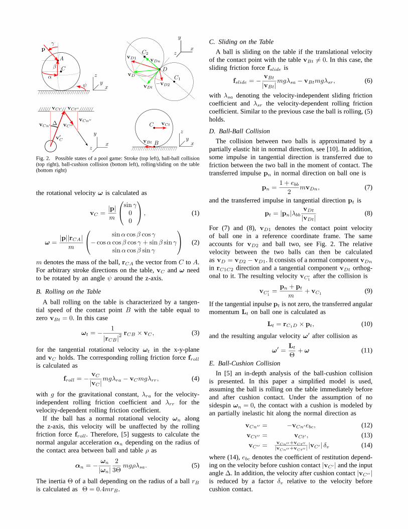
Fig. 2. Possible states of a pool game: Stroke (top left), ball-ball collision(top right), ball-cushion collision (bottom left), rolling/sliding on the table(bottom right)

the rotational velocityω is calculated as

vC =|p|

m

sin γ00

, (1)

ω =|p||rCA|

m

sinα cosβ cos γ− cosα cosβ cos γ + sinβ sin γ

sinα cosβ sin γ

(2)

m denotes the mass of the ball,rCA the vector fromC toA.For arbitrary stroke directions on the table,vC andω needto be rotated by an angleψ around the z-axis.

B. Rolling on the Table

A ball rolling on the table is characterized by a tangen-tial speed of the contact pointB with the table equal tozerovBt = 0. In this case

ωt = −1

|rCB |2rCB × vC , (3)

for the tangential rotational velocityωt in the x-y-planeandvC holds. The corresponding rolling friction forcefrollis calculated as

froll = −vC

|vC |mgλra − vCmgλrr, (4)

with g for the gravitational constant,λra for the velocity-independent rolling friction coefficient andλrr for thevelocity-dependent rolling friction coefficient.

If the ball has a normal rotational velocityωn alongthe z-axis, this velocity will be unaffected by the rollingfriction force froll. Therefore, [5] suggests to calculate thenormal angular accelerationαn depending on the radius ofthe contact area between ball and tableρ as

αn = −ωn

|ωn|

2

3Θmgρλsa. (5)

The inertiaΘ of a ball depending on the radius of a ballrBis calculated asΘ = 0.4mrB .

C. Sliding on the Table

A ball is sliding on the table if the translational velocityof the contact point with the tablevBt 6= 0. In this case, thesliding friction forcefslide is

fslide = −vBt

|vBt|mgλsa − vBtmgλsr, (6)

with λsa denoting the velocity-independent sliding frictioncoefficient andλsr the velocity-dependent rolling frictioncoefficient. Similar to the previous case the ball is rolling, (5)holds.

D. Ball-Ball Collision

The collision between two balls is approximated by apartially elastic hit in normal direction, see [10]. In addition,some impulse in tangential direction is transferred due tofriction between the two ball in the moment of contact. Thetransferred impulsepn in normal direction on ball one is

pn =1 + ebb

2mvDn, (7)

and the transferred impulse in tangential directionpt is

pt = |pn|λbbvDt

|vDt|(8)

For (7) and (8),vD1 denotes the contact point velocityof ball one in a reference coordinate frame. The sameaccounts forvD2 and ball two, see Fig. 2. The relativevelocity between the two balls can then be calculatedasvD = vD2 − vD1. It consists of a normal componentvDnin rC1C2 direction and a tangential componentvDt orthog-onal to it. The resulting velocityvC′

1after the collision is

vC′

1=

pn + pt

m+ vC1

(9)

If the tangential inpulsept is not zero, the transferred angularmomentumLt on ball one is calculated as

Lt = rC1D × pt, (10)

and the resulting angular velocityω′ after collision as

ω′ =

Lt

Θ+ ω (11)

E. Ball-Cushion Collision

In [5] an in-depth analysis of the ball-cushion collisionis presented. In this paper a simplified model is used,assuming the ball is rolling on the table immediately beforeand after cushion contact. Under the assumption of nosidespinωn = 0, the contact with a cushion is modeled byan partially inelastic hit along the normal direction as

vCn′′ = −vCn′ebc, (12)

vCt′′ = vCt′ , (13)

vC′′ = vCn′′+v

Ct′′

|vCn′′+v

Ct′′| |vC′ | δv (14)

where (14),ebc denotes the coefficient of restitution depend-ing on the velocity before cushion contact|vC′ | and the inputangle∆. In addition, the velocity after cushion contact|vC′′ |is reduced by a factorδv relative to the velocity beforecushion contact.

IV. PARAMETER DETERMINATION

For the model presented in Sec. III, the following parame-ters need to be determined:λra, λrr, λsa, λsr, λbb, ebb, ebc,δv, ρ, m, rB . Out of the 11 unknown physical parameters,the following 8 are evaluated:

1) Ball massm and radiusrB2) Rolling friction coefficientsλra andλrr3) Sliding friction coefficientsλsa andλsr4) Cushion parametersebc andδv

The other ones - namelyρ, λbb and ebb - cannot be de-termined due to too imprecise equipment and other super-imposed, more dominant effects. Here, values based on theresults of [5] and [10] are used.

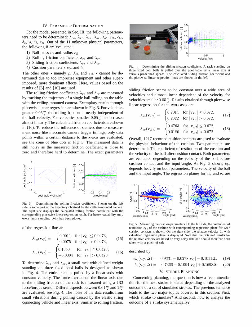
The rolling friction coefficientsλra andλrr are measuredby tracking the trajectory of a single ball rolling on the tablewith the ceiling-mounted camera. Exemplary results throughpiecewise linear regression are shown in Fig. 3. For velocitiesgreater 0.05m

sthe rolling friction is nearly independent of

the ball velocity. For velocities smaller 0.05ms

it decreasesalmost linearly. The calculated friction coefficients are shownin (16). To reduce the influence of outliers due to measure-ment noise like inaccurate camera trigger timings, only datapoints within a certain distance to the x-axis are evaluated,see the cone of blue dots in Fig. 3. The measured data isstill noisy as the measured friction coefficient is close tozero and therefore hard to determine. The exact parameters

−1 0 1−1

−0.5

0

0.5

1

pool table x−dim. [m]

pool

tabl

e y−

dim

. [m

]

0 0.2 0.4 0.6−0.04

−0.02

0

0.02

0.04

velocity [m/s]

fric

tion

coef

ficie

nt [−

]

Fig. 3. Determining the rolling friction coefficient. Shown on the leftside is some part of the trajectory obtained by the ceiling-mounted camera.The right side displays the calculated rolling friction coefficient with thecorresponding piecewise linear regression result. For better readability, onlyevery tenth sampling point has been plotted

of the regression line are

λra(vC) =

{

0.0011 for |vC | ≤ 0.0473,

0.0075 for |vC | > 0.0473,(15)

λrr(vC) =

{

0.1350 for |vC | ≤ 0.0473,

−0.0004 for |vC | > 0.0473(16)

To determineλsa andλsr, a small rack with defined weightstanding on three fixed pool balls is designed as shownin Fig. 4. The entire rack is pulled by a linear axis withconstant velocity. The force exerted on the linear axis dueto the sliding friction of the rack is measured using a JR3force/torque sensor. Different speeds between0.01m

sand1m

s

are evaluated, see Fig. 4. The noise of the data results fromsmall vibrations during pulling caused by the elastic stringconnecting vehicle and linear axis. Similar to rolling friction,

0 0.5 10

0.1

0.2

0.3

0.4

0.5

velocity [m/s]

fric

tion

coef

ficie

nt [−

]

Fig. 4. Determining the sliding friction coefficient. A rack standing onthree fixed pool balls is pulled over the pool table by a linearaxis atvarious predefined speeds. The calculated sliding frictioncoefficient andthe piecewise linear regression lines are shown on the left

sliding friction seems to be constant over a wide area ofvelocities and almost linear dependent of the velocity forvelocities smaller0.05m

s. Results obtained through piecewise

linear regression for the two cases are

λsa(vBt) =

{

0.2014 for |vBt| ≤ 0.672,

0.2322 for |vBt| > 0.672,(17)

λsr(vBt) =

{

0.4763 for |vBt| ≤ 0.672,

0.0180 for |vBt| > 0.672(18)

Overall, 1217 recorded cushion contacts are used to evaluatethe physical behaviour of the cushion. Two parameters aredetermined: The coefficient of restitution of the cushion andthe velocity of the ball after cushion contact. Both parametersare evaluated depending on the velocity of the ball beforecushion contact and the input angle. As Fig. 5 shows,ebcdepends heavily on both parameters: The velocity of the balland the input angle. The regression planes forebc andδv are

0.5 1 1.5 2 0 0.5 10

0.5

1

1.5

angle [rad]velocity [m/s]

CO

R [−

]

0.5 1 1.5 2 0 0.5 10

0.5

1

1.5

angle [rad]velocity [m/s]

rel.

velo

city

[−]

Fig. 5. Measuring the cushion parameters. On the left side, the coefficient ofrestitutionebc of the cushion with corresponding regression plane for 1217cushion contacts is shown. On the right side, the relative velocity δv withcalculated regression plane is displayed. Note that the obtained results forthe relative velocity are based on very noisy data and shouldtherefore beentaken with a pinch of salt

described by

ebc(vC ,∆) = 0.9331− 0.0278|vC | − 0.1051∆, (19)

δv(vC ,∆) = 0.7366− 0.1094|vC |+ 0.1698∆ (20)

V. STROKE PLANNING

Concerning planning, the question is how a recommenda-tion for the next stroke is stated depending on the analyzedoutcome of a set of simulated strokes. The previous sentenceleads to the two major topics covered in this section: First,which stroke to simulate? And second, how to analyze theoutcome of a stroke systematically?

A. Stroke Selection

When executing a stroke, one can varyα, β, γ, ψ andp. In order to reduce complexity and being able to makepredictions that can be transferred on a real pool table, onlytwo parameters are varied,p andψ. Implicitly it is assumedthe ball is hit centrally, i.e.α = 0, β = 0 and γ = π

2. For

this case, an optimal stroke angleψo is determined for eachobject ball - hole combination such that the object ball ispocketed in the mid of each pocket, see [19]. In addition,there are two anglesψ±h marking the maximal alloweddeviation to the left/right ofψo the ball is just pocketed,as shown in Fig. 6. If the angular deviation is bigger, oneis unable to pocket the object ball. Two other anglesψ±e

denote the angular deviation the object ball is just hit withoutmaking a foul. Similar limits exist for the stroke intensity: Anlower limit p−e the white ball is just fast enough to pocket theobject ball and an upper limitp+e depending on the robot’smaximal achievable velocity. As a result, one has only toconsider parameter tuples in a 2D search space betweenψ±e

andp±e assuming the robot is at least able to hit the objectball and programmed well enough to approximatep−e. Allcalculations can be extended to cover also possible obstacles(other balls) on the table.

ψ−eψ−h ψo ψ+h ψ+e

|p−e|

|p+e|

Rk+1n

pox

y

z

N(µ

|p|,σ2 |p

|)

N (µψ, σ2ψ)

ψ

|p|

Fig. 6. Calculation ofRk n. Assuming the robot is “skilled” enough,only sampling points withinψ±e and|p±e| are considered. Each samplingpoint has got an assigned valueRk+1n denoting the expected return for therobot from the next stroke on. Big blue dots indicate a high return for theplayer (positive) whereas big red dots mark a high return for the opponent(negative). ThenRk n is calculated based on an optimization overµ|p|andµψ . The optimization cost function is the average of all samplingpointsweighted withN (µ, σ2

|p|) andN (µψ , σ

2ψ). Under certain assumptions,µψ

can be set to a fixed value andµ|p| can be approximated with the centerof clusteredRk+1n values (black ellipse). In addition,po based upon theruled area marks the percentage to pocket the current ball if the outcomeof a stroke depends only on the angle

The robot’s (and opponent’s) skill is determined by a setof recorded sampling shots with measured angular deviationrelative to ψo and measured intensity deviation relativeto a predefined value. Both values are approximated bynormal distributionsN (µψ, σ

2ψ) for the angular deviation

andN (µ|p|, σ2

|p|) for the impulse deviation. Neglecting thestroke intensity, the percentagepo to pocket an object ballis calculated based on the approximated normal distributionof the angular deviation andψ±e.

B. Planning Ahead

In order to analyze the strokes, skilled human players alsoconsider the most likely situations for the nextn strokesbeside the current situation. A situation on the table attime k in the future is described as a stateX containingthe positions of theN balls on the table, whereX isthe Cartesian productX = x1 × x2 × . . .× xN , where thesets xi are subsets ofR2 giving the space of possiblepositions of the i-th ball on the table. Thenwk is thecost associated with the stateXk determining how good orbad the situation is for the player. Similar to reinforcementlearning problems as described in [15] and [24] we modelthis effect with an discounted finite-horizon return functionwith discount factorδ:

R0n =

n∑

k=0

δkwk, 0 ≤ δ < 1 (21)

Let us assume an arbitrary finite sequence of strokes resultingin a sequence(X0, . . . , Xn) and consequently a sequence ofstates returns(w0, . . . , wn). The returnwk is defined as +1 ifthe player pockets a ball and 0 otherwise. For the opponent,the reward is -1 if he pockets a ball and 0 otherwise. Becausethe outcome of each stroke is probabilistic, one has toweight every possible stroke outcome with its correspondingprobability depending on the impulsep and angleψ andintegrate over all probabilitiesp(p, ψ):

R0n =

n∑

k=0

[

δk∫∫

wk p(p, ψ) dψdp

]

, δ ∈ R+ (22)

For δ = 1, there is a proper physical understanding ofR0n,as aR0n value greater zero indicates the player is going topocket more balls over the nextn rounds than the opponentfrom a statistical point of view. The opposite applies forR0n

values smaller than zero. Consequently, the resulting goalforthis planning problem is formulated as

maximizep,ψ,stroke sequence

(R0n) (23)

The first step in solving (23) is to discretize the problemand to set up a search tree of depthn where each nodeof depth k = 1 . . . n represents the situation on the tableafterk strokes. When sampling the 2D search space of eachnode, one also has to consider the possible outcome for theopponent. When simulating a robot stroke of depthk in thetree and the shot parameter are withinψ±h and |p±e|, therobot can continue playing the next round. Iteratively, onegets new search spaces of depthk + 1. The same accountsfor the opponent of depthk + 1 if the shot parameters arewithin ψ±h andψ±e and |p±e|. If the maximum depthn isreached, we do not plan another step ahead. In this case,Rnnis a single scalar number representing the maximal percent-age to pocket a ballpmaxP for the robot respectivelypmaxOfor the opponent.

Subsequently, an optimization algorithm is used varyingthe stroke intensityµ|p| and stroke angleµψ variables ofeach node of the tree in order to solve (23). This problem isintractable within reasonable for large search trees as there

areO((ns)n) variables to optimize forns sampling points

for each table and a search tree of depthn.However, experiments show that under certain assump-

tions a good approximate solution is obtained. Except for ex-tremely easy shots or very skilled pool players andδ . 1, µψis close toψo after optimization. This abandons the need tooptimize for µψ. The physical interpretation is that exceptfor those situations the primary goal is to pocket the objectball in the most simple manner, thus by aiming at the centerof the pocket. In addition, optimization forµ|p| is bypassedby assigning a value to each sampling point in the searchspace of a node of depthk equal toRk+1n, whereRk+1n

represents the return function for the subtree starting fromthe specific sampling point on. The resulting search spacewith sampling points and corresponding valuesRk+1n isthen clustered using the OPTICS algorithm [25], taking onlya fraction of the bestRk+1n values into account. Everyfound cluster withµ|p| set to the center of the cluster is com-pared with each other, making it possible to calculateRk nas the average return based onN (µψ, σ

2ψ), N (µ|p|, σ

2

|p|)and Rk+1n via backward induction. After having iteratedto the root of the search tree,R0n will return the optimalvaluesµψ andµ|p| for the next shot.

C. Safety Shots

Pool offers another element of strategic gameplay calledsafety shots. After having announced a safety shot, the op-ponent will continue with the next shot in any case. Lookingat the search tree, because we now have to consider twodifferent possibilities for each situation, the number of nodesin the tree grows fromO((ns)

n) to O((ns)2n). This is the

brute-force approach. A more elegant solution first analyseseach situation and then decides dynamically whether one alsowants to consider a safety shot. In general, there are tworeasons for announcing a safety shot in roundk:

1) There is no chance for the robot of executing a legalstroke after the next stroke. We reduce this situation tothe case the robot can’t hit any object ball.

2) The situation after the next shot will be bad for bothrobot and opponent.

With respect toR0n and the game logic, not announcinga safety shot in the first case will result in comitting a foulthe next round, thus letting the opponent place the white balltwo rounds ahead whereever he wants. As this is assumed tobe optimal for the opponent, it is always better to announcea safety shot. For the second case, announcing a safety shotmeans expecting a high return in the long run with thedisadvantage of letting intentionally execute the opponent theshot after the next round. Here, the expected returnRk+1n

for any subtree starting from depthk+1 without announcinga safety shot is close to zero and a safety shot may lead tobetter results.

VI. RESULTS

Measuringµψ, σψ, µ|p| and σ|p| for any player (humanor robot) is achieved by a set of recorded sample strokes.Regarding the stroke intensity, this can be adjusted and

measured precisely for the robot. On the other hand, humanplayers are told to pocket a set of balls with “light intensity”,“normal intensity” and “high intensity”. As the standarddeviations for all three cases were quite similar, a singlevalue has been used instead. However, this fact has to beconsidered if the planner is ought to be used for humans.

−1 −0.5 0 0.5 1

−0.6

−0.4

−0.2

0

0.2

0.4

0.6

x−dimension [m]

y−

dim

ensio

n [m

]

87%

98%

−1 −0.5 0 0.5 1

−0.6

−0.4

−0.2

0

0.2

0.4

0.6

x−dimension [m]

y−

dim

ensio

n [m

]

R2 = 1.34

−0.32 0 0.320

0.2

0.4

0.6

angular deviation [deg]

impuls

e [N

s]

−0.32 0 0.320

0.2

0.4

0.6

angular deviation [deg]

impuls

e [N

s]

−1 −0.5 0 0.5 1

−0.5

0

0.5

x−dimension [m]

y−

dim

ensio

n [m

]

−1 −0.5 0 0.5 1

−0.5

0

0.5

x−dimension [m]

y−

dim

ensio

n [m

]

R1 = 1.28

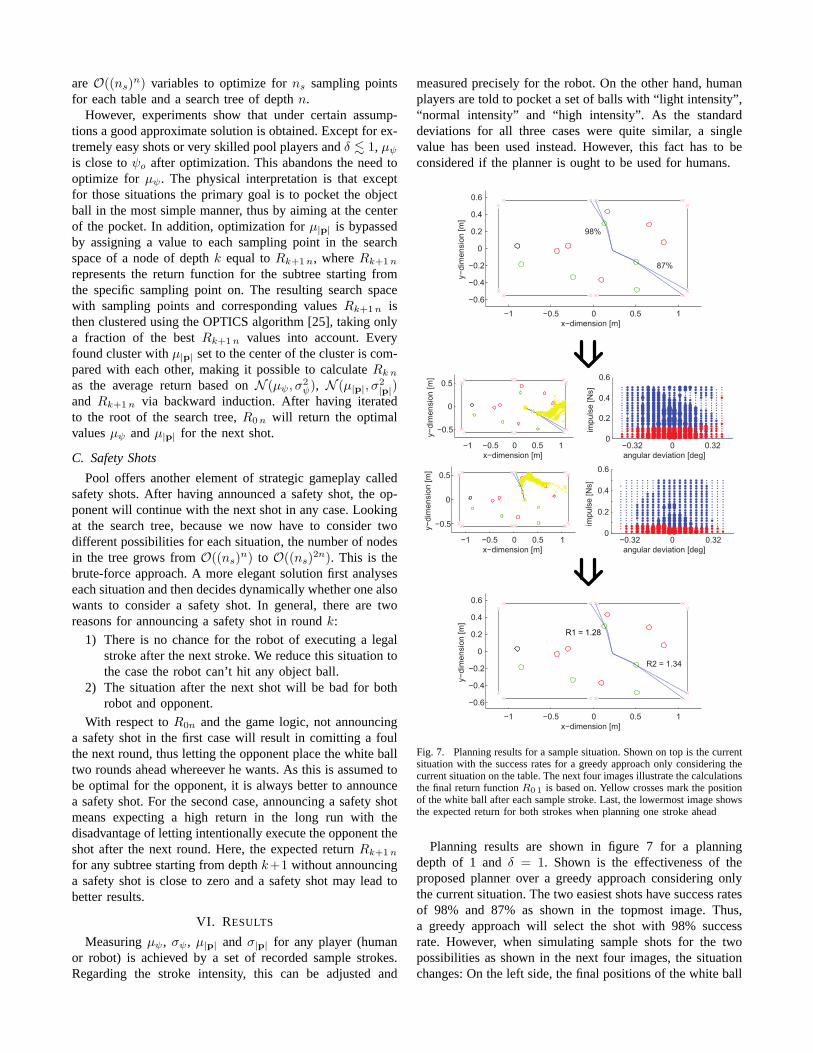
Fig. 7. Planning results for a sample situation. Shown on top is the currentsituation with the success rates for a greedy approach only considering thecurrent situation on the table. The next four images illustrate the calculationsthe final return functionR0 1 is based on. Yellow crosses mark the positionof the white ball after each sample stroke. Last, the lowermostimage showsthe expected return for both strokes when planning one stroke ahead

Planning results are shown in figure 7 for a planningdepth of 1 andδ = 1. Shown is the effectiveness of theproposed planner over a greedy approach considering onlythe current situation. The two easiest shots have success ratesof 98% and 87% as shown in the topmost image. Thus,a greedy approach will select the shot with 98% successrate. However, when simulating sample shots for the twopossibilities as shown in the next four images, the situationchanges: On the left side, the final positions of the white ball

after having executed a set of sample shots are marked witha yellow cross. The right side displays the search space thatis used to calculateR0 1. Because the tree depth equals 1,everyR1 1 value represents the maximal percentage to pocketa ball in the next round for the player (blue dots) if he pocketsthe object ball without a foul or for the opponent (red dots).The lowermost image shows the resultingR0 1 values forboth strokes, indicating that it is advantageous to pocket theball with the lower success rate as it has the higher expectedreturn.

VII. D ISCUSSION

As many aspects of pool are already analyzed in detail,most topics of this paper can be compared in a broadercontext. To a large extent our pool simulator model isfounded on well established physical principles. For the ball-cushion collision, the resulting equations are extended tomodel the physical effects for the given pool table better.It is not our intention to model every physical effect asaccurate as possible (e.g. spin), rather we concentrate on thedominant, measurable and best understood effects. Differingfrom other pool simulator implementations, this planner usesnumerical integration instead of an analytical solution forbetter modeling of discontinuous friction effects (as shownin Sec. IV) and easier model improvement whenever newmeasurements are available.

With respect to the planner presented in this paper, thediscounted return approach in combination with modeledstroke angle and impulse deviation is promising as parametertuning is reduced to choose a suitable discount factorδ thatdetermines the look-ahead horizon of the planning strategy.One still existing problem covers end game situations whereone or two players have only few balls left. Because theplanner does not depend explicitly on the number of ballsas shown in (22), a potentially desired shift in the playingstrategy cannot be accomodated adequatly.

VIII. C ONCLUSION

This paper presents a framework for a robotic pool playingsystem with advanced planning capabilities. Particular em-phasis is on the interactive playing capability with a humanopponent requiring for a tight coupling and real-time capa-bility of perception, planning, and stroke execution. Based ona unified approach, we are able to handle tactical decisionsduring a pool game including the consideration of differentplayer strengths. Whereas the current implementation is tiedto the pool game, the general idea can be extended to variousepisodic games in order to include human capabilities intothe robot’s tactical considerations.

ACKNOWLEDGEMENT

This work is supported in part within the DFG excellenceresearch clusterCognition for Technical Systems - CoTeSys(www.cotesys.org).

REFERENCES

[1] T. Weigel and B. Nebel, “Kiro - an autonomous table soccer player,”in In Proc. Int. RoboCup Symposium 02. Springer-Verlag, 2002, pp.119–127.

[2] http://www.robocup.org.[3] Y. H. Zhang, W. Wei, D. Yu, and C. W. Zhong, “A tracking and

predicting scheme for ping pong robot,”Journal of Zhejiang University- Science C, vol. 12,no.2, pp. 110–115, 2011.

[4] W. Leckie and M. Greenspan, “An event-based pool physicssimula-tor,” ACG 2005, Taipei, Taiwan, September 6-9, pp. 247–262, 2006.

[5] I. Han, “Dynamics in carom and three cushion billiards,”Journal ofMechanical Science and Technology, vol. 19, no.4, pp. 976–984, 2005.

[6] R. Shepard. (1997) Amateur physics for the amateur pool player.[Online]. Available: http://www.tcbilliards.com/articles/physics.shtml

[7] A. Salazar and A. Sanchez-Lavega, “Motion of a ball on a roughhorizontal surface after being struck by a tapering rod,”EuropeanJournal of Physics, vol. 11, pp. 228–232, 1990.

[8] S. C. Crown, “Modeling the effects of velocity, spin, frictional coef-ficient, and impact angle on deflection angle in near-elastic collisionsof phenolic resin spheres,” 2004.

[9] J. H. Bayes and W. T. Scott, “Billard-ball collision experiment,”American Journal of Physics, vol. 31, no.3, pp. 197–200, 1963.

[10] R. E. Wallace and M. C. Schroeder, “Analysis of billiardball collisionsin two dimensions,”American Journal of Physics, vol. 56, no.9, pp.815–819, 1988.

[11] D. Gugan, “Inelastic collision and the hertz theory of impact,” Amer-ican Journal of Physics, vol. 68, no.10, pp. 920–924, 1999.

[12] R. Cross, “Cue and ball deflection in billiards,”American Journal ofPhysics, vol. 76, no.3, pp. 205–212, 2007.

[13] M. de la Torre Juarez, “The effect of impulsive forces on asystemwith friction: the example of the billiard game,”European Journal ofPhysics, vol. 15, pp. 184–190, 1994.

[14] Carom3d. [Online]. Available: http://www.carom3d.com[15] M. Smith, “Pickpocket: A computer billiards shark,”Artif. Intell., vol.

171, pp. 1069–1091, 2007.[16] C. Archibald, A. Altman, and Y. Shoham, “Analysis of a winning

computational billiards player,” inProceedings of IJCAI, 2009, pp.1377–1382.

[17] M. Smith, “Running the table: An ai for computer billiards,” Interna-tional Computer Games Association Journal, vol. 56, no.9, pp. 191–193, 2004.

[18] Z. M. Lin, J.-S. Yang, and C. Y. Yang, “Grey decision-making for abilliard robot,” in Proceedings of SMC (6), 2004.

[19] J.-F. Landry and J.-P. Dussault, “Ai optimization of a billiard player,”Journal of Intelligent and Robotic Systems, vol. 50, pp. 399–417, 2007.

[20] J.-P. Dussault and J.-F. Landry, “Optimization of a billiard player -tactical play,” inComputers and Games’06, 2006.

[21] D. Brscic, M. Eggers, F. Rohrmuller, O. Kourakos, S. Sosnowski,D. Althoff, M. Lawitzky, A. Mortl, M. Rambow, V. Koropouli, J. M.Hernandez, X. Zang, W. Wang, D. Wollherr, K. Kuhnlenz, C. Mayer,T. Kruse, A. Kirsch, J. Blume, A. Bannat, T. Rehrl, F. Wallhoff,T. Lorenz, P. Basili, C. Lenz, T. Roder, G. Panin, W. Maier, S. Hirche,M. Buss, M. Beetz, B. Radig, A. Schubo, S. Glasauer, A. Knoll, andE. Steinbach, “Multi joint action in cotesys - setup and challenges,”CoTeSys Cluster of Excellence: Technische Universitat Munchen &Ludwig-Maximilians-Universitat Munchen, Munich, Germany, Tech.Rep. CoTeSys-TR-10-01, June 2010.

[22] D. Althoff, O. Kourakos, M. Lawitzky, A. Mortl, M. Rambow,F. Rohrmuller, D. Brscic, D. Wollherr, S. Hirche, and M. Buss,“An architecture for real-time control in multi-robot systems,” inHuman Centered Robot Systems, ser. Cognitive Systems Monographs.Springer Berlin Heidelberg, 2009, vol. 6, pp. 43–52.

[23] T. Nierhoff, O. Kourakos, and S. Hirche, “Playing pool with a dual-armed robot,” in International IEEE Conference on Robotics andAutomation, 2010, pp. 3445 – 3446.

[24] R. S. Sutton and A. G. Barto,Reinforcement Learning: An Introduc-tion. MIT Press, 1998.

[25] M. Ankerst, M. M. Breunig, H.-P. Kriegel, and J. Sander,“Optics:Ordering points to identify the clustering structure.” ACMPress,1999, pp. 49–60.