Strategic Leniency and Cartel Enforcement∗

Nathan H. Miller†

University of California - Berkeley

September 2007

Abstract

The cornerstone of cartel enforcement in the United States and elsewhere is a com-mitment to the lenient prosecution of early confessors. A burgeoning game-theoreticalliterature is ambiguous regarding the impacts of leniency. I develop a theoretical modelof cartel behavior that provides empirical predictions and moment conditions, and ap-ply the model to the complete set of indictments and information reports issued over atwenty year span. Reduced-form statistical tests are consistent with the notion that le-niency enhances deterrence and detection capabilities. Direct estimation of the model,via the method of moments, yields a 59 percent lower cartel formation rate and a 62percent higher cartel detection rate due to leniency. The results have implications formarket efficiency and criminal enforcement.

Keywords: cartel enforcement, leniency program, amnesty, organized crimeJEL classification: K4, L4

∗This paper was previously circulated under the title Can Strategic Leniency Fight Organized Crime:Empirical Evidence from Cartel Enforcement. I am grateful to my advisor, Richard Gilbert, for his adviceand patience. I also thank Judith Chevalier, Joseph Farrell, Russell Pittman, John Sutton, Sofia Villas-Boas,Gregory Werden, Catherine Wolfram, two anonymous referees, and seminar participants at the Universityof California, Berkeley and the Department of Justice for valuable comments. The Institute of Business andEconomic Research provided financial support.

†Department of Economics, University of California-Berkeley, 512 Evans Hall #3800, Berkeley, CA 94720-3880.

“The data obstacle to addressing these questions is that we only observe discov-ered cartels, so we do not know the frequency of cartels in the economy. Until wefind a way in which to surmount that obstacle, the ultimate impact of leniencyprograms on cartel formation and the duration of cartels will remain an openquestion.”

∼ Joseph E. Harrington (forthcoming)

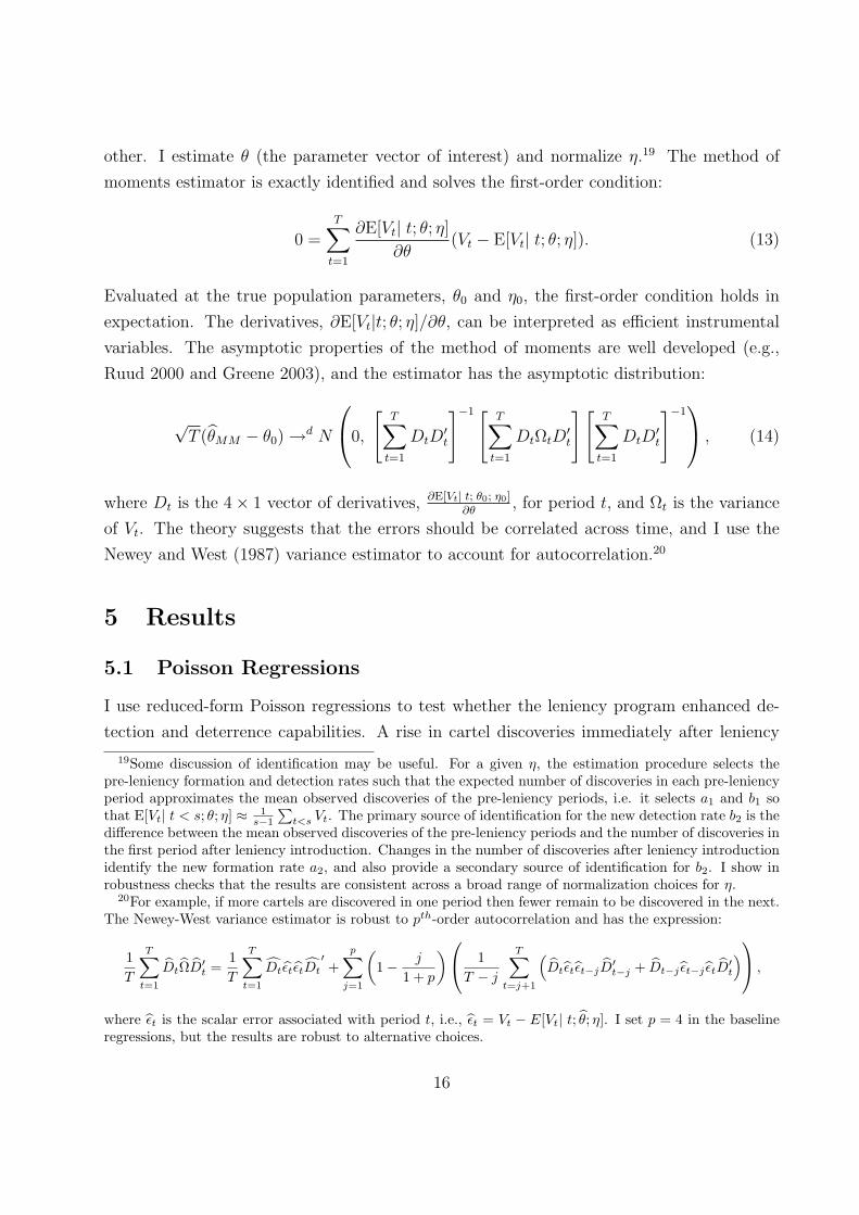
1 Introduction

In 1993, the Department of Justice (DOJ) introduced a new leniency program, with the

intent of destabilizing existing cartels and deterring new cartels. The program commits the

DOJ to the lenient prosecution of early confessors. In particular, it guarantees complete

amnesty from federal prosecution to the first confessor, provided that an investigation is not

already underway. It also offers discretionary penalty reductions to conspirators (both firms

and employees) that confess when an investigation is already ongoing. The new leniency

program has become the cornerstone of cartel enforcement efforts in the United States (e.g.,

Hammond 2004) and has recently inspired antitrust authorities in Australia, Canada, the

European Union, Japan, South Korea, and elsewhere to introduce similar programs (OECD

2002, 2003). This paper tests the efficacy of the new leniency program. The results have

implications for market efficiency and enforcement efforts against cartels and other forms of

organized crime.

A burgeoning game-theoretical literature is ambiguous regarding the impacts of le-

niency. A common finding is that leniency may destabilize cartels because conspirators can

simultaneously cheat on the collusive arrangement and apply for leniency (e.g., Spagnolo

2004, Chen and Harrington 2007, Harrington forthcoming). Leniency also may destabilize

cartels when conspirators can exploit the policy to raise rivals’ costs in subsequent peri-

ods (Ellis and Wilson 2001). Alternatively, leniency may stabilize some types of collusive

arrangements (e.g., Spagnolo 2000, Ellis and Wilson 2001, Chen and Harrington 2007), and

may even encourage new cartels to form when detection probabilities change stochastically

because firms anticipate smaller penalties in the event of detection (Motta and Polo 2003,

Harrington forthcoming). The effects of leniency also may depend on market concentra-

tion (Ellis and Wilson 2003), whether fines are proportional to accumulated cartel profits

(Motchenkova 2004), and the degree of firm heterogeneity (Motchenkova and van der Laan

2005). In virtually all the models, the effects of leniency hinge on specific parameters, the

1

values of which are unknowable theoretically and difficult to estimate empirically.1

This paper provides the first independent empirical evaluation of leniency in cartel

enforcement, as applied in the United States.2 Much of our extant knowledge regarding

the efficacy of the new leniency program comes from DOJ Antitrust Division officials, who

consistently laud the program:

The Amnesty Program is the Division’s most effective generator of large cases,and it is the Department’s most successful leniency program (Spratling 1999).

To put it plainly, cartel members are starting to sweat, and the amnesty programfeeds off that panic (Hammond 2000).

It is, unquestionably, the single greatest investigative tool available to anti-cartelenforcers (Hammond 2001).

Because cartel activities are hatched and carried out in secret, obtaining thecooperation of insiders is the best... way to crack a cartel (Pate 2004).3

It may be prudent to view this rhetoric with some degree of skepticism. The game-

theoretical literature suggests that antitrust authorities have incentives to over-represent

their enforcement capabilities because leniency is more powerful when firms anticipate only

short-lived cartel profits (e.g., Hinloopen 2003, Motchenkova 2004, Chen and Harrington

2007). The DOJ attempts to manage firm perceptions for exactly this reason:

antitrust authorities must cultivate an environment in which business executivesperceive a significant risk of detection by antitrust authorities if they enter into,or continue to engage in, cartel activity (Hammond 2004).

Moreover, the DOJ maintains strict confidentiality regarding the identity of amnesty appli-

cants (e.g., Spratling 1999).4 Although it is possible to make inferences in some cases, more

commonly the identity (or even existence) of a leniency applicant is unknowable from publicly

1Rey (2003) and Spagnolo (2006) provide excellent summaries of this theoretical literature. On a relatedsubject, Spagnolo (2004) and Aubert, Rey and Kovacic (2006) note that rewarding confessors may enhanceenforcement capabilities.

2Brenner (2005) evaluates the efficacy of the 1996 European Commission leniency notice. I discuss hismethodology and results below.

3Gary R. Spratling was Deputy Assistant Attorney General in 1999. Scott D. Hammond is DeputyAssistant Attorney General and served as Director of Criminal Enforcement in 2000 and 2001. R. HewittPate is Assistant Attorney General.

4Thus, for example, when the DOJ prosecutes a firm for price-fixing violations it does not list co-conspirators by name in the publicly available legal documents.

2

available data. The combination of potentially perverse incentives and lack of institutional

transparency motivates this analysis.

I develop a theoretical model of cartel behavior that helps overcome the difficulty,

common to all empirical research on collusion, that active cartels are never observed in

the data. Specifically, I analyze a first-order Markov process in which industries transition

stochastically between collusion and competition. I show how changes in the rate at which

cartels form and the rate at which they are discovered affect the expected time-series of cartel

discoveries. The model generates intuitive empirical predictions that can be used to assess the

efficacy of antitrust innovations (such as the leniency program). In particular, an immediate

increase in cartel discoveries following an innovation is consistent with enhanced detection

capabilities, and a subsequent readjustment below pre-innovation levels is consistent with

enhanced deterrence capabilities. The model also supplies moment conditions that can

identify the formation and detection rates in more structural estimation.

I take the theoretical model to the complete set of indictments and information reports

issued by the DOJ between January 1, 1985 and March 15, 2005.5 I use these documents to

construct a time-series of cartel discoveries. The introduction of the new leniency program

on August 10, 1993 provides an exogenous shock that identifies the effect of leniency on

cartel formation and detection rates. Before that date, the DOJ offered leniency only on a

discretionary basis and only before an investigation had started. Whereas the DOJ received

only seventeen leniency applications between 1978 and 1993, it has averaged roughly one

application per month since (e.g., Bingaman 1994, Spratling 1999, Hammond 2003).

I pursue two complementary empirical strategies. First, I use reduced-form Poisson

regression to test whether cartel discoveries increase immediately following leniency intro-

duction (consistent with enhanced detection) and whether discoveries subsequently fall below

initial levels (consistent with enhanced deterrence). I am able to control for economic con-

ditions, the budget of the Antitrust Division, and other factors that may influence cartel

discoveries. Second, I exploit functional forms supplied by the theoretical model to identify

the formation and detection rates, and I estimate these parameters directly via the method

of moments. The econometric procedure selects formation and detection rates that mini-

mize the “distance” between the time-series of cartel discoveries predicted by the theoretical

model and the time-series of discoveries observed in the data. The procedure helps quantify

the specific impact of leniency on detection and deterrence capabilities.

By way of preview, the time-series of cartel discoveries is consistent with the notion

5An information reports does not require a grand jury and is typically filed in conjunction with a pleaagreement from one or more defendants.

3

that the introduction of the new leniency program enhanced the detection and deterrence

capabilities of the DOJ. The number of discoveries increases immediately following the le-

niency introduction and then falls below pre-leniency levels. Reduced-form statistical tests

indicate that the changes are statistically significant under a number of alternative sample

and specification choices. More structural estimation, based on the minimum distance pro-

cedure, yields a 59 percent decrease in the cartel formation rate and a 62 percent increase

in the cartel detection rate in response to leniency introduction. The results lend credence

to the DOJ rhetoric and indicate that leniency programs may have the intended effects.

The analysis is subject to at least two important caveats, and the results may best be

interpreted with caution. The first caveat is that the theoretical model requires one to draw

inferences about the pool of undiscovered cartels with information gleaned from discovered

cartels. Valid inference is possible so long as discovered cartels are representative in some

fashion. I assume that the antitrust authority discovers all cartels with equal probability.

The assumption is not testable, though I show in an appendix that the theoretical predic-

tions regarding cartel discoveries are robust to alternative assumptions. The second caveat

is that the regression sample is essentially a single time-series with one exogenous policy

change. Cross-sectional variation could provide more robust identification, and the recent

introduction of leniency programs by other antitrust authorities may provide this variation

for future studies. Early evidence suggests that the experience of the United States may

generalize. For example, the European Commission revised its leniency program in 2002 to

include automatic amnesty for the first confessor. The Commission received leniency appli-

cations in more than twenty cases during the first year of the revised program, relative to

only sixteen cases during the previous six years combined (Van Barlingen 2003).

The paper makes three separate contributions to the literature. First, I develop a

theoretical model that guides the empirical evaluation of the new leniency program. The

model is fairly intuitive and general, and may help facilitate the evaluation of other criminal

enforcement efforts, both in antitrust and (potentially) in other settings characterized by

unobservable criminal action and observable detection. Second, I construct and analyze

data on cartels discovered between 1985 and 2005. The descriptive statistics may be of

some interest to antitrust economists. To my knowledge, no other work has analyzed cartel-

level data from the United States since Bryant and Eckard (1991). Finally, I interpret

the data within the framework of the theoretical model and show that the time-series of

cartel discoveries is consistent with the notion that the new leniency program increased the

detection and deterrence capabilities of the DOJ.

Independently, Harrington and Chang (2007) develop an alternative framework with

4

which to test the efficacy of cartel enforcement innovations. Their framework differs from

the one developed here namely in that it generates empirical predictions for the time-series

of observed cartel durations, rather than for the time-series of discoveries.6 Unfortunately,

empirical applications of the Harrington and Chang (2007) framework may be frustrated

by measurement problems associated with reported durations. For example, conventional

wisdom holds that the start and end dates of collusive activity reported by the DOJ may

be negotiated as part of a plea agreement, and that the DOJ may devote little effort to

accurately identifying determine the true end date of collusion so long as prosecution can

proceed within the statute of limitations. The theoretical model developed here may have

advantages to the extent that cartel discoveries are more cleanly measured.

The empirical results most closely relate to those of Brenner (2005), who shows that

the initial introduction of leniency within the European Union in 1996 had little discernable

effect on the duration of detected cartels. As discussed above, the European Commission

did not guarantee amnesty to first confessors until 2002. Thus, assuming away the mea-

surement problems associated with cartel durations, Brenner’s results are consistent with

those presented here because they suggest that guaranteed amnesty to first confessors may

be an important component of successful leniency programs. Other related empirical work

includes that of Ghosal and Gallo (2001) and Ghosal (2004), which documents the relation-

ships between antitrust caseloads and various political and economic factors.

The results may have important market efficiency implications. Cartels are generally

thought to expropriate consumer surplus and create deadweight welfare loss. Although

criminal law treats collusion as per se illegal, the data analyzed here indicate that the DOJ

detected cartels in more than 200 distinct industries over the sample period. The price effects

of this collusion appear large. Connor (2004) and Connor and Bolotova (2005) calculate a

median overcharge of 28 percent, based on meta-analysis of more than 600 cartels. The

estimate is similar to those reported in a spate of case studies (e.g., Howard and Kaserman

1989, Froeb, Koyak and Werden 1993, Kwoka 1997, Porter and Zona 1999, Connor 2001,

White 2001).7

The results also may be relevant to law enforcement efforts against organized crime

generally. Spagnolo (2000, 2004) shows that the incentives that govern cartel behavior are

quite similar to those that govern gang activities, long-term corruption, and drug trafficking.

In each, the lack of enforceable contracts may create free riding, hold-up, and moral haz-

6Harrington and Chang (2007) show that effective antitrust innovations raise the average duration ofdetected cartels in the short run by discouraging the operations of less stable (and shorter-lived) cartels.

7Whinston (2006) provides an overview of this literature.

5

ard problems, and conspirators may employ long-term relationships to support cooperation.

Relationships may also generate evidence that one or more conspirators can sell to enforce-

ment authorities in exchange for lenient treatment. In principle, therefore, the theoretical

literature on strategic leniency and the empirical results presented here may extend to other

forms of organized crime.

Of course, the application of strategic leniency to the problem of organized crime is

not novel. Nearly 23 percent of drug traffickers sentenced by U.S. courts in fiscal year 2005

received sentences shorter than the mandatory minimum in exchange for testimony and/or

other incriminating evidence against co-conspirators in line with the U.S. Sentencing Guide-

lines (U.S. Sentencing Commission 2005). However, these grants of leniency are generally

negotiated ex post and at the discretion of the prosecuting authority. The results presented

here suggest that the provision of automatic leniency under a set of transparent and well-

advertised conditions may strengthen the ability of criminal enforcement agencies to deter

and detect organized criminal behavior.

The paper proceeds as follows. Section 2 introduces the model of industry behavior

and derives empirical predictions and moment conditions. Section 3 discusses the data

construction, provides summary statistics, and motivates the regression sample. Section 4

outlines the empirical strategies. Section 5 presents the main results and robustness checks.

Section 6 provides an early empirical analysis of the European Commission’s 2002 Leniency

Notice. Section 7 concludes.

2 The Theoretical Model

2.1 Industry behavior

Assume that an antitrust authority enforces competition, albeit imperfectly, in n = 1, 2, . . . N

industries over t = 1, 2, . . . periods. Industries collude or compete in each period, and may

change states between periods. Industries that compete during period t collude during the

next period with probability at. The antitrust authority discovers industries that collude

(cartels) during period t with probability bt and these industries compete in the subsequent

period. Cartels that avoid discovery abandon collusion for other reasons with probability ct.

The transition parameters at, bt and ct can be interpreted as the formation rate, the detection

rate, and the dissolution rate, respectively, and are determined outside of the model. Each

must lie along the open interval between zero and one. For notational reasons discussed

6

below, let the parameter vector θ = (at, bt) and the parameter vector η = (ct, N).8

The setup imbeds two simplifying assumptions that help generate clean predictions.

First, the system is memoryless in the sense that the length of time an industry operates in

the collusive or competitive states does not affect the transition probabilities. This property

is testable and I show in Section 5 that the data provide some support. Second, the industries

are identical and independent, in the sense that industries share transition probabilities and

the transitions of one industry have no effect on other industries. In an appendix, I examine

a deterministic game-theoretical model, akin to that of Spagnolo (2004), and show that the

main predictions of the theoretical model are robust to industry-level heterogeneity.

2.2 A steady state in expectations

The distribution of industries across the collusive and competitive states follows a first-order

Markov process in expectations and, provided that the transition parameters are constant,

the distribution converges to a steady state regardless of initial conditions. Further, closed-

form expressions for both the steady state and the path of convergence are available.

To start, denote the number of industries that start colluding after period t as Ut, the

number of cartels that the antitrust authority detects after period t as Vt, and the number of

cartels that abandon collusion after period t as Wt. These “flow” quantities each sum a series

of identical industry-specific Bernoulli events and have binomial distributions characterized

by the relevant transition parameter(s) and the pre-existing distribution of industries across

the collusive and competitive states (e.g., Casella and Berger 2002):

Ut ∼ binomial(Yt, at), E[Ut] = atYt,

Vt ∼ binomial(Xt, bt), E[Vt] = btXt,

Wt ∼ binomial(Xt − Vt, ct), E[Wt] = ct(1− bt)Xt,

(1)

where Xt and Yt denote the number of industries that collude and compete during period t,

respectively. Thus, for example, the expected number of discoveries after period t is simply

the detection rate times the number cartels active during period t.

Equation 1 yields a distribution of industries across the collusive and competitive states

that follows a first-order Markov process in expectations:

8In Appendix B, I show that these assumptions correspond to a reduced-form version of the economicmodel employed by Harrington (forthcoming).

7

E

[Xt+1

Yt+1

]=

[1− bt − ct(1− bt) at

bt + ct(1− bt) 1− at

]E

[Xt

Yt

]. (2)

The process, like all Markov processes governed by transition probabilities strictly bounded

between zero and one, converges to a unique steady state provided that the probabilities are

fixed across periods. The steady state vector, [X∗ Y ∗]′, has the expression:

[X∗

Y ∗

]= 1

a+b+c(1−b)

[a

b + c(1− b)

]N. (3)

Convergence to the steady state vector occurs regardless of the initial conditions. Consider

the arbitrary vector [Xt Yt]′. The numbers of firms that collude and compete, respectively,

in expectation during period t + τ (τ > 0) have the closed form expressions:

E[Xt+τ ] =a

a + b + c(1− b)

(1 +

b + c(1− b)

a(1− a− b− c(1− b))τ

)Xt

+a

a + b + c(1− b)

(1− (1− a− b− c(1− b))τ

)Yt ,

E[Yt+τ ] =a

a + b + c(1− b)

(b + c(1− b)

a− b + c(1− b)

a(1− a− b− c(1− b))τ

)Xt

+a

a + b + c(1− b)

(b + c(1− b)

a+ (1− a− b− c(1− b))τ

)Yt. (4)

These convergence paths are obtainable via difference equations, and I sketch the algebraic

steps in Appendix A. It may be apparent, however, that as τ trends to infinity, the expected

state vector E[Xt+τ Yt+τ ]′ converges to the steady state vector [X∗ Y ∗]′.

2.3 The Number of Cartel Discoveries

An antitrust innovation, such as the leniency policy, affects the number of cartels that the

antitrust authority discovers over time. I model an antitrust innovation as an exogenous

change in the formation and/or detection rates during the arbitrary period t = s. I hold the

dissolution rate and the number of industries constant, though I relax these constraints in

the empirical application.9

9Appendix B shows that leniency has ambiguous implications for the dissolution rate. The intuition issimple. Consider an effective leniency program that destabilizes cartels. It might (or might not) be optimalfor firms that abandon collusion to apply simultaneously for leniency, depending on the extent of leniencyand the probability of detection. The extent to which the firms choose to apply for leniency determineswhether the dissolution rate increases or decreases. For now, I hold the dissolution rate constant to improve

8

Equations 1 and 3 give the expected steady state number of cartel discoveries prior to

the innovation:

E[Vt| t < s; θ; η] =b1a1

a1 + b1 + c(1− b1)N, (5)

where a1 and b1 represent the formation and detection rates prior to the innovation. After

the innovation, the expected number of cartel discoveries converges to:

limt→∞

E[Vt| θ; η] =b2a2

a2 + b2 + c(1− b2)N, (6)

where a2 and b2 represent the new formation and detection rates. Equations 1 and 4 give

the path of convergence:

E[Vt| t ≥ s; θ; η] =b2a2

a2 + b2 + c(1− b2)

(1 +

b2 + c(1− b2)

a2

(1− a2 − b2 − c(1− b2))t−s

)X∗

1

+b2a2

a2 + b2 + c(1− b2)

(1− (1− a2 − b2 − c(1− b2))

t−s

)Y ∗

1 . (7)

To help build intuition, Figure 1 plots the expected convergence paths after four differ-

ent innovations. Panels A and B isolate changes in the detection and formation rates, respec-

tively. In particular, Panel A features an increase in the detection rate (b1 = 0.2, b2 = 0.3)

and holds the other parameters constant (N = 100, a1 = a2 = 0.2, c = 0.0). The number

of expected cartel discoveries is higher immediately following the innovation because the

antitrust authority discovers a greater proportion of active cartels, but this effect dampens

as the enhanced detection shrinks the pool of active cartels. By contrast, Panel B features a

decrease in the formation rate (a1 = 0.2, a2 = 0.1) and holds the other parameters constant

(N = 100, b1 = b2 = 0.2, c = 0.0). There is no immediate change but discoveries again fall

gradually as enhanced deterrence shrinks the pool of active cartels.

[Figure 1 about here.]

Panels C and D combine simultaneous changes in the detection and formation rates.

Panel C features an increase in the detection rate (b1 = 0.2, b2 = 0.3) and a decrease in

the formation rate (a1 = 0.2, a2 = 0.1), and holds the other parameters constant (N =

100, c = 0.0). The changes may be characteristic of “successful” innovations in that they

are consistent with enhanced detection and deterrence capabilities. The number of expected

cartel discoveries is higher immediately following the innovation due to the detection rate

the tractability of the theoretical model. The empirical application deals flexibly with the issue.

9

increase. The detection and formation rate changes both shrink the pool of active cartels

over time, so discoveries then fall accordingly. Discoveries fall below initial levels because

the formation rate decrease is sufficiently large. Panel D features a decrease in the detection

rate (b1 = 0.2, b2 = 0.15) and an increase in the formation rate (a1 = 0.2, a2 = 0.4), and

holds the other parameters constant (N = 100, c = 0.0). The changes may be characteristic

of “failed” innovations. Discoveries drop initially and then rise above initial levels.

These expected convergence paths provide the intuition that underlies the main results:

Result 1: An immediate rise in the expected number of cartel discoveries after an innovation

is sufficient to establish an increase in the detection rate.

Result 2: If expected discoveries rise immediately after an innovation then a subsequent

readjustment below initial levels is sufficient to establish a decrease in the formation rate.

I provide proofs in Appendix A. The theoretical results have the empirical analogues that an

immediate increase in cartel discoveries following the introduction of the leniency program is

consistent with enhanced detection capabilities, and that a subsequent readjustment below

pre-leniency levels is consistent with enhanced deterrence capabilities. Additionally, the

expected path of discoveries – as expressed in Equations 5 and 7 – provides a moment that

can be exploited for direct estimation of the parameters.

3 Data and Sample Information

3.1 Data construction

The data consist of all indictments and information reports filed for violations of Section 1

of the Sherman Act between January 1, 1985 and March 15, 2005.10 Information reports do

not require a grand jury and are typically filed in conjunction with plea agreements from

one or more defendants. The DOJ saves resources by issuing information reports rather

than indictments, which may help explain why the data include 809 information reports

versus 222 indictments. Each document – regardless of whether it is an indictment or an

information report – includes the name of the alleged conspirator, the affected geographic

and product markets, and approximate start and end dates of the conspiracy, as well as

various other information.

10Documents filed after December 1, 1994 are available for download from the DOJ Antitrust Divisionwebsite, <www.usdoj.gov/atr/cases.htm>.

10

The documents do not typically provide a one-to-one map to the cartels: many cartels

appear to result in two or more documents, and many documents list multiple firms and/or

individuals that participated in a single cartel. I group the conspirators into cartels to

facilitate evaluation on the cartel level. The procedure is necessarily ad hoc because the DOJ

does not explicitly identify co-conspirators across documents. Nonetheless, the groupings

may be reasonably accurate due to the wealth of geographic, product, and temporal data.11

In ex post comparisons, the groupings match well various cartel descriptions provided by the

DOJ. I identify a total of 343 distinct cartels.

3.2 Sample statistics

Table 1 contains summary statistics for the duration, geographic scope, industry classifi-

cation, and size of the cartels. The average cartel lasts for 4.61 years, when duration is

measured as the difference between the start and end dates estimated by the DOJ. Because

this duration measure may contain substantial noise, I calculate an upper bound as the time

in years between the start and indictment dates. This upper bound has a sample mean of

6.98 years. Interestingly, the means of both measures are quite similar to those calculated

by Bryant and Eckard (1991) for cartels prosecuted between 1961 and 1988.12

[Table 1 about here.]

To describe the geographic scope of the cartels, I create three dummy variables that

equal one if the affected market is local, regional, or at least national, respectively. I define

local markets as those that are strictly contained within a single state, regional markets as

those that include all of a state and/or parts of multiple states, and national markets as

those that span a more substantial proportion of the country. As shown, 43 percent of the

cartels operated in local markets, 34 percent operated in regional markets and 23 percent

operated in national markets. The documents do not specify whether the affected geographic

market is international in scope but do provide the headquarters of prosecuted firms. Nine

percent of the sample cartels include an international firm.

11As discussed below, the regression sample minimizes grouping errors.12Some of the estimated start and end dates are not specific but rather designate only a month or, worse,

only a year. I choose the earliest date within the specified range as the start date and the latest date as theend date. For example, if the listed start and end date is “May 2000,” I use May 1, 2000 as the start dateand May 31, 2000 as the end date. Estimated start and end dates for a given cartel sometimes differ acrossdocuments. Again, I use the earliest start date and the latest end date. I proxy the end date with the filingdate when the end date is missing.

11

Next, I map the DOJ product market descriptions into the North American Industry

Classification System (NAICS). As shown the sample cartels are evenly spread among the

construction, manufacturing, wholesale trade, retail trade, and “other” industries. Finally,

the DOJ prosecuted a mean of 3.24 firms per cartel. Of course, the DOJ may not prosecute all

conspirators, due to leniency or other reasons. To pursue this idea further, Table 2 provides

the empirical distribution of firms prosecuted. The DOJ pursued legal action against only

one firm in fully thirty percent of the cases despite the fact that, by definition, cartels require

the participation of multiple firms.13

[Table 2 about here.]

Table 3 provides split-sample means, based on whether the document’s filing date

predated or postdated the introduction of the new leniency program on August 10, 1993.

Two changes appear to be first-order. First, the number of cartel discoveries drops from 218

before leniency (on average, 25.65 per year) to 125 after leniency introduction (on average,

10.64 per year). Second, cartels detected in the later period tend to be broader in geographic

scope – the fraction of cartels that were local decreased from 50 percent to 31 percent, the

fraction that were national increased from 12 percent to 41 percent, and the fraction with

an international firm increased from 1 percent to 23 percent. Difference-in-means t-statistics

indicate statistical significance in each case. These changes could be due to the leniency

program, expanding market boundaries, and/or other factors that affect cartels or cartel

enforcement.

[Table 3 about here.]

3.3 The regression sample

The theoretical model develops predictions and moment conditions for the number of cartel

discoveries and the duration of these cartels. I create a series of six-month periods to track

these factors. The periods alternately begin on August 10 and February 10, so that they fit

the introduction of the new leniency program on August 10, 1993. There are forty periods

in the data and I calculate the number of discoveries and the average duration of discovered

cartels in each.14 I include only the first cartel discovery per industry in the calculations (207

13The empirical distributions before and after leniency introduction are similar: The DOJ pursued legalaction against only one firm in 31 percent of the cases prior to the leniency program and in 30 percent ofthe cases after the introduction of leniency.

14I drop three cartels that have filing dates before February 10, 1985 or after February 9, 2005. I show inrobustness checks that the main results are robust to the use of three- and twelve-month periods.

12

cartels qualify). Subsequent intra-industry discoveries would, if included, threaten observa-

tional independence because the DOJ often parlays discoveries into information regarding

related cartels. The sample selection rule also minimizes any mistakes associated with the

ad hoc grouping procedure because it avoids double-counting when a single-industry cartel

is erroneously classified as two (or more) distinct cartels.15

Panel A of Figure 2 plots the number of discoveries per six-month period over the sam-

ple. The vertical bar represents the introduction of the new leniency program. Discoveries

average 6.3 per period prior to leniency without an apparent trend. Discoveries are higher

in the periods surrounding leniency introduction. The final pre-leniency period features nine

discoveries, and the first two leniency periods feature ten and nine discoveries, respectively.

Discoveries average 3.7 over the remaining periods. Within the framework of the theoretical

model, the surge in discoveries around leniency introduction is suggestive of enhanced detec-

tion capabilities, and the subsequent drop in discoveries is suggestive of enhanced deterrence

capabilities.16

[Figure 2 about here.]

The remaining panels of Figure 2 explore the sample selection rule in greater detail.

Panel B plots total discoveries per six-month period, inclusive of all cartels. Total discoveries

trend downward over the sample period, to the extent that the comparative statics of the

theoretical model are of second-order magnitude at best. The downward trend may be

related to the broadening of geographic scope observed over the sample period: a cartel that

operates across several geographic markets leaves less room for other cartels in the same

industry to operate. Consistent with this logic, the cartels excluded by the sample selection

rule are 67.65 percent more likely to operate in a local geographic market than included

cartels. Further, Panels C and D show that local cartels and excluded cartels, respectively,

trend downwards together over the sample period. In robustness checks, I show that the

15The sample selection rule simply sharpens the research question: I focus on whether leniency affectsthe ability of the DOJ to detect independent cartels rather than whether leniency facilitates intra-industrydiscoveries. For robustness, I experiment with more strict sample selection rules. The results are similarwhen I exclude cartels with a previously indicted conspirator and/or cartels whose discovery is known tohave been influenced by previous investigations in different industries (e.g., the DOJ discovered the sodiumgluconate cartel through its investigation of the citric acid cartel). Notably, the results do not depend onthe inclusion/exclusion of the Akzo Nobel and Archer Daniels Midland cartels discovered over the course ofthe 1990s.

16Discoveries jump the period before introduction of the leniency program, which suggests that cartelsmay have anticipated the introduction of the program. I explore this possibility in Section 5. The resultsare robust to various treatments of the final pre-leniency period.

13

empirical methodology can accommodate total discoveries, and that the main results hold

under this accommodation.

4 Empirical Framework

4.1 Poisson Regression

I use reduced-form Poisson regression to test whether the data are consistent with changes

in the formation and detection rates after the introduction of the leniency program. The

regression model expresses the probability that Vt, the number of cartel discoveries, has the

realization vt as:

Prob(Vt = vt | xt) =exp(−λt)λ

vtt

vt!, zt = 0, 1, 2, . . . , (8)

where the conditional mean λt is:

λt = exp(x′tβ), (9)

the vector xt contains regressors, and β is a vector of parameters. The regressors include

LENIENCY, which equals 1 if the period postdates the introduction of leniency and 0 oth-

erwise, as well as polynomials in TIME1 and TIME2. The variable TIME1 equals 1 during

the first period, 2 during the second period, and so on. The variable TIME2 equals 1 in the

second period following leniency introduction, 2 in the next period, and so on.17

I perform two statistical tests. In the first, I examine whether the number of cartel

discoveries increases immediately after the introduction of leniency. Result 1 of the theoret-

ical model suggests that such an increase is consistent with enhanced detection capabilities.

Because the regression model generates an immediate increase in discoveries if and only if

the LENIENCY coefficient is positive, I test the hypothesis:

H0 : βLEN ≤ 0 versus H1 : βLEN > 0, (10)

where βLEN denotes the LENIENCY coefficient. In the second statistical test, I examine

17Two econometric issues are worthy of mention. The Poisson regression model provides consistent esti-mates even when the dependent variable is not generated specifically from a Poisson process (e.g., Cameronand Trivedi 1998). The model is thus suitable for analyzing discoveries, which are distributed binomial byEquation 1. Also, statistical inference is valid under the assumption of equidispersion, i.e., the equality of theconditional mean and the conditional variance. For robustness, I estimate more flexible negative binomialregression models and show that the data fail to reject the equidispersion assumption.

14

whether the number of cartel discoveries subsequently decreases below initial levels. Result 2

of the theoretical model suggests that such a decrease is consistent with enhanced deterrence.

In the regression model, changes in the number of discoveries correspond to changes in the

conditional mean. Thus, I test the hypothesis:

H0 : λt|t>>s ≥ λs versus H1 : λt|t>>s < λs, (11)

where λ is the condition mean and s is the period of leniency introduction.

For robustness, I estimate the Poisson regression model controlling for potentially con-

founding influences. Ghosal and Gallo (2001) suggest that the DOJ caseload may be counter-

cyclical and positively associated with the Antitrust Division budget allocation, and I create

variables that proxy these factors. The first variable, ∆GDP, is the semi-annual growth rate

of the real gross domestic product. The second variable, FUNDS, is the average Antitrust

Division budget allocation. I also create the variable FINES, which captures total corpo-

rate fines issued by the Antitrust Division during the previous fiscal year. The means of

the three variables are 0.015, 0.088, and 0.128, respectively, though I demean the variables

before estimation to ease interpretation.18

4.2 Direct Estimation

I employ the method of moments to select the formation and detection rates that minimize

the distance between the time-series of cartel discoveries predicted by the theoretical model

and the time-series of discoveries observed in the data. The estimator is:

θMM = arg minθ∈Θ

1

T

T∑t=1

(Vt − E[Vt| t; θ; η])2, (12)

where Vt is the number of discoveries during period t, E[Vt|t; θ; η] is the expected number of

discoveries, as defined by Equations 5 and 7, the parameter vector θ includes the formation

and detection rates, and the parameter vector η contains the dissolution rates and the number

of industries. The functional form of E[Vt| t; θ; η] identifies either θ or η as a function of the

18The data are available from the Antitrust Division website (<www.usdoj.gov/atr/public/10804a.htm>and <http://www.usdoj.gov/atr/public/workstats.htm>) on a fiscal year basis. I define FUNDS as theweighted-average of the budget allocations for periods that include two fiscal years. I lag FINES in order tomitigate potential endogeneity issues. Both FUNDS and FINES are measured in billions of real 2000 dollars.The main results hold when the control variables enter in logarithmic form.

15

other. I estimate θ (the parameter vector of interest) and normalize η.19 The method of

moments estimator is exactly identified and solves the first-order condition:

0 =T∑

t=1

∂E[Vt| t; θ; η]

∂θ(Vt − E[Vt| t; θ; η]). (13)

Evaluated at the true population parameters, θ0 and η0, the first-order condition holds in

expectation. The derivatives, ∂E[Vt|t; θ; η]/∂θ, can be interpreted as efficient instrumental

variables. The asymptotic properties of the method of moments are well developed (e.g.,

Ruud 2000 and Greene 2003), and the estimator has the asymptotic distribution:

√T (θMM − θ0) →d N

0,

[T∑

t=1

DtD′t

]−1 [T∑

t=1

DtΩtD′t

][T∑

t=1

DtD′t

]−1 , (14)

where Dt is the 4× 1 vector of derivatives, ∂E[Vt| t; θ0; η0]∂θ

, for period t, and Ωt is the variance

of Vt. The theory suggests that the errors should be correlated across time, and I use the

Newey and West (1987) variance estimator to account for autocorrelation.20

5 Results

5.1 Poisson Regressions

I use reduced-form Poisson regressions to test whether the leniency program enhanced de-

tection and deterrence capabilities. A rise in cartel discoveries immediately after leniency

19Some discussion of identification may be useful. For a given η, the estimation procedure selects thepre-leniency formation and detection rates such that the expected number of discoveries in each pre-leniencyperiod approximates the mean observed discoveries of the pre-leniency periods, i.e. it selects a1 and b1 sothat E[Vt| t < s; θ; η] ≈ 1

s−1

∑t<s Vt. The primary source of identification for the new detection rate b2 is the

difference between the mean observed discoveries of the pre-leniency periods and the number of discoveries inthe first period after leniency introduction. Changes in the number of discoveries after leniency introductionidentify the new formation rate a2, and also provide a secondary source of identification for b2. I show inrobustness checks that the results are consistent across a broad range of normalization choices for η.

20For example, if more cartels are discovered in one period then fewer remain to be discovered in the next.The Newey-West variance estimator is robust to pth-order autocorrelation and has the expression:

1T

T∑t=1

DtΩD′t =

1T

T∑t=1

DtεtεtDt

′+

p∑

j=1

(1− j

1 + p

) 1

T − j

T∑

t=j+1

(Dtεtεt−jD

′t−j + Dt−j εt−j εtD

′t

) ,

where εt is the scalar error associated with period t, i.e., εt = Vt − E[Vt| t; θ; η]. I set p = 4 in the baselineregressions, but the results are robust to alternative choices.

16

introduction is consistent with establish enhanced detection capabilities. A subsequent read-

justment below initial levels is consistent with enhanced deterrence capabilities.

Starting with detection, Table 4 presents the main Poisson regression results. In each

regression, the units of observation are six-month periods and the dependent variable is the

number of cartel discoveries. Column 1 includes LENIENCY and a fifth-order polynomial

in TIME2. The estimated LENIENCY coefficient of 0.474 corresponds to an immediate

60.66 percent increase in discoveries and is statistically significant at the one percent level,

consistent with enhanced detection. Columns 2, 3, and 4 feature different polynomials

in TIME1 and TIME2. Specifically, Column 2 includes a first-order polynomial in TIME1,

Column 3 includes a fourth-order polynomial in TIME2, and Column 4 includes a sixth-order

polynomial in TIME2. The estimated LENIENCY coefficients correspond to immediate

71.88, 60.90, and 59.12 percent increases in discoveries, respectively, and the coefficients

remain statistically significant in each case.21

[Table 4 about here.]

Table 5 shows that the result is robust to the inclusion of control variables and the

use of different period lengths. Columns 1, 2, and 3 alternately include ∆ GDP, FUNDS,

and FINES, and Column 4 includes all four control variables. The estimated LENIENCY

coefficients remain positive and statistically significant, and correspond to immediate 54.86,

83.79, 61.48, and 61.33 percent increases in discoveries, respectively, when evaluated at the

mean of the control variables. Interestingly, the results provide little support for the empirical

findings of Ghosal and Gallo (2001) that antitrust activity is countercyclical and correlated

with the Antitrust Division budget. Columns 4 and 5 use three-month periods and twelve-

month periods, respectively. The estimated LENIENCY coefficients remain positive and

significant, and correspond to immediate 89.52 and 46.98 percent increases in discoveries.22

[Table 5 about here.]

Turning to deterrence, Figure 3 plots the estimated conditional means (i.e., predicted

values) for the regressions shown in Table 4, along with 95 percent confidence intervals for

21Valid statistical inference in the Poisson regression model depends on equidispersion, i.e., the equality ofthe conditional mean and variance. For robustness, I estimate the more flexible negative binomial regressionmodel. The coefficients are virtually identical to those obtained from the Poisson regression. The dispersionparameter is nearly zero and a likelihood ratio test fails to reject the null of equidispersion (p-value= 0.50).

22Ghosal and Gallo (2001) and Ghosal (2004) show that the party of the President may correlate withDOJ antitrust case activity. The data studied here indicate that Republican administrations discovered anaverage of 10.58 cartels per year (including only the first cartel per industry) versus an average of 10.00per year for Democrat administrations. The small number of regime changes (two) hampers meaningfulidentification of any party effects within the Poisson regression framework.

17

the estimates. Panel A includes LENIENCY and fifth-order polynomial in TIME2. The

predicted value for periods before the leniency program is 6.47. Following the post-leniency

spike in discoveries, the predicted values quickly fall below this level, consistent with greater

deterrence capabilities. The differences are statistically significant and large in magnitude:

the mean predicted value for periods at least three years after leniency introduction is 3.78,

which corresponds to a 41.61 percent reduction relative to pre-leniency levels. Panels B, C,

and D feature different polynomials in TIME1 and TIME2. Panel B includes a first-order

polynomial in TIME1, Panel C includes a fourth-order polynomial in TIME2, and Pane

D includes a sixth-order polynomial in TIME2. In each case, the predicted values after

leniency quickly fall below the pre-leniency level. The mean predicted values for periods at

least three years after leniency are 37.53, 41.60, and 41.67 percent lower than pre-leniency

levels, respectively, and the differences remain statistically significant.23

[Figure 3 about here.]

Figure 4 shows that the result is robust to the inclusion of control variables and the

use of different period lengths. Panels A, B, and C alternately include ∆ GDP, FUNDS,

and FINES, and Panel D includes all four control variables. In each case, the predicted

values after leniency fall below the pre-leniency level. The mean predicted values for periods

at least three years after leniency are 42.54, 5.10, 44.87, and 38.95 percent lower than pre-

leniency levels, respectively, when evaluated at the mean of the control variables. The

differences are statistically significant in each case.24 Panels E and F use three-month and

twelve-month periods, respectively. Again, the predicted values after leniency fall below

the pre-leniency levels. The mean predicted values for periods at least three years after

leniency are 41.03 and 41.21 percent lower than pre-leniency levels, and the differences are

statistically significant. Overall, the results provide statistical support for enhanced detection

and deterrence capabilities due to the introduction of the new leniency program.

[Figure 4 about here.]

23Significance at the five percent level is maintained for all periods, with the exceptions of the final periodin Panel C and the final three periods in Panel D.

24Significance at the five percent level is maintained for all periods in Panels A and C, for one periodin Panel B and for six periods in Panel D. In general, the results are somewhat weaker when a control forthe Antitrust Division budget is included. The budget trends upwards during the sample but has littleyear-to-year variation: the regression of FUNDS on a linear time trend yields an R2 of 0.9352.

18

5.2 Direct Estimation

Table 6 presents the results of direct estimation, via the method of moments, for a specific

set of normalization choices. I let the total number of industries (N) be 1,000 and let the

dissolution rates before and after leniency introduction (c1 and c2) be 0.40. As shown, the

estimated cartel formation rate falls from 0.0156 before leniency to 0.0064 after leniency

introduction. The difference of −0.0092 is statistically significant and represents a 59.20

percent reduction. The estimated detection rate rises from 0.2297 to 0.3714. The difference

of 0.1416 is statistically significant and represents a 61.65 percent increase. Each of the

parameters is precisely estimated. Figure 5 plots the regression fit against the data. The

estimation procedure fully captures the increase in discoveries around leniency introduction

as well as the subsequent downward adjustment. The result is consistent with substantial

effects of leniency on the ability of the DOJ to deter and detect cartels.25

[Table 6 about here.]

[Figure 5 about here.]

Table 7 shows that the results are consistent across different normalization choices.

Column 1 features a lower constant dissolution rate (c1 = c2 = 0.30), Column 2 features

a higher constant dissolution rate (c1 = c2 = 0.50), Column 3 features a dissolution rate

increase following leniency introduction (c1 = 0.40, c2 = 0.50), Column 4 features a disso-

lution rate decrease (c1 = 0.50, c2 = 0.40), Column 5 features fewer industries (N = 500),

and Column 6 features more industries (N = 3, 000). In each case, the minimum distance

procedure suggests that the formation rate fell and the detection rate rose following leniency

introduction, and that the changes are statistically significant. In percentage terms, the

magnitude of the effects are quite similar across columns – the estimated reduction in the

formation rate ranges from 55.80 to 64.34 percent, and the estimated increase in the detection

rate is close to 61.60 percent in each column.26

25The standard errors account for fourth-order autocorrelation (p = 4) ala Newey and West (1987). Thedata suggest that autocorrelation may indeed be present: an OLS regression of the Table 6 residuals εt onthe lagged residuals εt−1, . . . , εt−4 returns coefficients of −0.49, −0.56, −0.47, and −0.18, consistent withnegative autocorrelation. Further, the test statistic TR2 = 12.73 exceeds the χ2

4,0.95 critical value of 9.49, sothe data reject the null of zero autocorrelation (Breusch 1978, Godfrey 1978). The main results are robustto alternative choices of p, including p = 0.

26The parameter estimates differ across columns in absolute terms. At least two effects merit discussion.First, the overall magnitude of the estimated formation and detection rates change with the normalizeddissolution rate (e.g., Column 1 vs. Column 2). Because the dissolution rate is fundamentally unidentifiable,the estimation procedure cannot identify the rate magnitudes (by contrast, the rate changes are robustly

19

[Table 7 about here.]

Table 8 shows that the results are similar across a number of robustness regressions.

First, to account for potentially confounding influences, I use Poisson regression to remove

the variance in cartel discoveries due to economic growth, the Antitrust Division budget

allocation, and the magnitude of corporate fines, and then use these adjusted discoveries as

the dependent variable in the minimum distance procedure.27 Column 1 presents the results.

The formation rate falls from 0.0138 before leniency to 0.0056 after leniency introduction.

The difference is statistically significant and represents a 59.06 percent reduction. The

detection rate rises from 0.2741 to 0.4411. The difference is statistically significant and

represents a 60.90 percent increase. Together, the findings suggest that the main results

may reflect real change rather than spurious correlations.

[Table 8 about here.]

Next, I consider alternative period lengths. Columns 2 and 3 present estimation results

based on three-month and twelve-month periods, respectively. Again, the formation rates

fall after the introduction of leniency. The changes are statistically significant and represent

71.60 and 55.70 percent reductions. Similarly, the detection rates increase after leniency in-

troduction. The changes are statistically significant and represent 1.0482 and 0.5477 percent

increases. Thus, alternative period lengths do not appear to substantially affect the direction

of the main results, but the estimated rate changes are somewhat larger in magnitude with

shorter periods.

In Column 4, I relax the assumption that the number of industries is constant over the

sample period. The formation and detection rate parameters remain identifiable provided

that some growth pattern is specified. I estimate the model under the assumption that the

number of industries is subject to constant proportional growth. That is, I let the number

of industries be:

N = n ∗ exp(ρ ∗ TIME1), (15)

identified). Second, the estimated formation rates are higher when the smaller number of industries is smaller(Column 5 vs. Column 6). This is exactly what one would expect from the estimation procedure becausethe formation rate and the number of industries act as substitutes in the maintenance of a cartel pool of agiven size.

27I use Poisson regression to model the number of discoveries as a function of LENIENCY, a fifth-orderpolynomial in TIME2, an intercept, and the control variables (∆ GDP, FUNDS, and FINES), as in Table5, Column 4. I then calculate the predicted values, evaluated at the means of the control variables, and theresiduals. The sum of these two measures is the adjusted number of discoveries and serves as the dependentvariable in the direct estimation of the formation and detection rates.

20

where n is the base number of industries and ρ is the constant growth rate. The growth

rate is identifiable and its estimation provides a specification test: the flexible model is

equivalent to the baseline model only when ρ = 0.28 As shown, estimation based on the

familiar normalization choices n = 1, 000 and c1 = c2 = 0.40 yields a growth parameter

that is small (ρ = −0.0074) but precisely estimated (standard error = 0.0013). The findings

regarding the formation and detection rates are similar to those of the baseline regressions,

although the formation rate decrease is somewhat smaller (53.83 percent) and the detection

rate increase is somewhat larger (72.41 percent).

Finally, the assumption of constant proportional industry growth makes estimation

based on total discoveries (inclusive of all cartels) feasible. Column 5 presents the results

of this estimation. The growth rate is negative (ρ = −0.0283) and statistically significant

(standard error = 0.0014), and accounts for the downward trend in total discoveries over the

sample period. Again, the findings regarding the formation and detection rates are similar

to those of the baseline regressions, although the formation rate decrease and the detection

rate increase are somewhat smaller in magnitude (41.23 and 28.09 percent, respectively).

The findings provide some comfort in that the main results are robust to different sample

selection treatments. In particular, one need not restrict attention to the first cartel in each

industry to generate the main results.

5.3 Remaining Issues

5.3.1 Did cartels anticipate the leniency program?

An interesting feature of the data is that discoveries actually spike prior to the introduction

of the leniency program. At first glance, one is tempted to explain the spike as an antici-

pation effect. The data are not supportive. Of the twelve cartels discovered in the period

immediately preceding leniency, nine were discovered more than three months prior to intro-

duction. The Assistant Attorney General who introduced the program – Anne Bingaman –

was appointed fewer than two months prior to introduction. Nonetheless, I regress discov-

eries on LENIENCY and a fourth-order polynomial in TIME2, excluding the period before

leniency. The resulting Poisson regression coefficient of 0.499 is statistically significant at

the one percent level. I also redefine LENIENCY and TIME2 as if the leniency program was

introduced one period sooner (i.e., on February 10, 1993). The resulting coefficient of 0.487

is again statistically significant at the one percent level. Thus, the main findings appear to

28The growth parameter is identified primarily by trends in discoveries over the pre-leniency periods.

21

be robust to different treatments of this particular pre-leniency period.29

5.3.2 Is the spike in cartel discoveries just noise?

The results weigh heavily the increase in cartel discoveries surrounding the introduction of

leniency. However, the data are noisy and discoveries also seem higher than trend in some

periods that predate the leniency program (Figure 2, Panel D). A skeptic might argue that

the concurrence of leniency introduction and a spike in discoveries could reasonably exist in

the data due to pure chance. In order to assess the likelihood of this possibility, I redefine

LENIENCY and TIME2 as if the leniency program was introduced during earlier periods.

In particular, I focus on the spike that occurs in period eleven (February 10 to August 9,

1990). I regress the number of discoveries on LENIENCY and a fifth-order polynomial in

TIME2, as in Column 1 of Table 4. The LENIENCY coefficient is relatively small (0.300)

and is not statistically significant (t-stat= 1.07), which suggests that the spike in discoveries

surrounding the true date of leniency introduction is somewhat distinctive and may not be

the result of pure chance.

More generally, the estimation procedure depends on the exogenous imposition of Au-

gust 10, 1993 as a structural breakpoint. It is natural to question the robustness of the

breakpoint, especially given the spike in discoveries preceding leniency introduction. In par-

ticular, one might suspect that the empirical model may be misspecified to the extent that

alternative breakpoints better fit the data. To address this concern, I redefine LENIENCY

and TIME2 as if the leniency program was introduced in other periods, and then regress

the number of discoveries on LENIENCY and a fifth-order polynomial in TIME2 for each

possible breakpoint. The fit of the regression – as measured by the pseudo-R2 – is maximal

when the breakpoint is imposed on August 10, 1993, which suggests that the data can deliver

the correct breakpoint.

29Alternatively, one might expect firms to delay their leniency applications until the introduction of thenew leniency program, in which case the empirical model would overestimate the impact of the new leniencyprogram on the detection rate. The empirical evidence cuts against this story. To the extent that firmsdelayed leniency applications, two patterns should be present in the data. First, the number of discoveriesshould be low immediately prior to the introduction of the new leniency program. Second, the number ofdiscoveries should drop quickly between the first and second periods after leniency introduction (as opposedto the more gradual fall implied by the theoretical model). Neither holds in the data. The number ofdiscoveries is high before leniency introduction and remains high through the second period after leniencyintroduction.

22

5.3.3 Does the probability of detection depend on time in state?

The theoretical model is memoryless, in the sense that the length of time an industry operates

in the collusive or competitive states does not affect the transition probabilities. The property

helps generate clean predictions and is particularly important for the duration moments. Yet

it may fail in the data, especially to the extent that the DOJ levies more substantive fines

on longer-lived cartels. To examine the memoryless property empirically, I test the null

hypothesis that the probability of detection is constant in the duration of collusion, i.e., that

cartels face a constant hazard rate. The memoryless property implies that cartel duration has

the exponential distribution. I estimate a Weibull model via maximum likelihood and test

whether the shape parameter equals one – under that constraint, the Weibull distribution

collapses to an exponential and features a constant hazard rate. Estimation on the regression

sample yields a shape parameter of 0.9826, and a likelihood ratio test fails to reject the null

hypothesis that the underlying population parameter equals one.30

5.3.4 Do civil damages matter?

On June 22, 2004, President Bush signed the Antitrust Criminal Penalty Enhancement

and Reform Act (ACPERA), which de-trebled civil damages for amnesty recipients.31 One

might expect the number of cartel discoveries to increase following that date. To investigate,

I extend the sample through July 2007. Figure 6 plots the results, using ten six-month

periods between June 22, 2002 and June 22, 2007. As shown, there is no discernable increase

in discoveries immediately following the introduction of ACPERA. The results suggest that

the ACPERA may have little substantial impact on detection capabilities.

[Figure 6 about here.]

6 Preliminary Evidence from the European Union

The European Commission’s 2002 Leniency Notice may facilitate further empirical evalu-

ations of strategic leniency. The 2002 Leniency Notice is analogous to the new leniency

30I measure cartel duration as the difference in years between the start and end dates, as estimatedby the DOJ. The results are similar for cartels discovered before and after leniency, respectively. As analternative approach, I consider the empirical cumulative distribution function of observed cartel durations,F (D) = (number of cartels with duration < D)/(total number of cartels). Under the memoryless property,log(1 − F (D)) should be approximately linear in D (e.g., Bryant and Eckard 1991). The relationship isindeed approximately linear: the OLS regression of log(1− F (D)) on cartel duration yields an adjusted R2

of 0.9944. Bryant and Eckard (1991) report similar results for cartel discoveries over the period 1961-1988.31Hammond (2005) provides a detailed description of the ACPERA.

23

program in the United States because both guarantee immunity to confessors that report

before an investigation opens and offer potential fine reductions to confessors that report

after an investigation opens. Furthermore, both replaced regimes in which immunity grants

were discretionary and relatively ineffective in inducing cooperation from members of pre-

viously undetected cartels.32 In principle, therefore, one could use the methods outlined in

Sections 2 and 4 to sign and measure the effect of the 2002 Leniency Notice on the ability

of the Commission to detect and deter cartels.

The Commission publishes non-confidential versions of its antitrust decisions on its

website.33 The documents are richer than the indictments and information reports made

available by the DOJ. Each uniquely identifies a single cartel and its conspirators, so that

ad hoc grouping across documents is unnecessary. The documents provide the date(s) of

any leniency application(s) as well as the dates of “dawn raids” and information requests.

They specify explicitly whether the investigation was initiated in response to a leniency

application. The documents also provide case results, including which firms qualified for

full/partial leniency, the aggravating and attenuating circumstances, and the fines levied

against each conspirator. As in the DOJ indictments and information reports, the documents

list the affected geographic and product markets and approximate start and end dates.

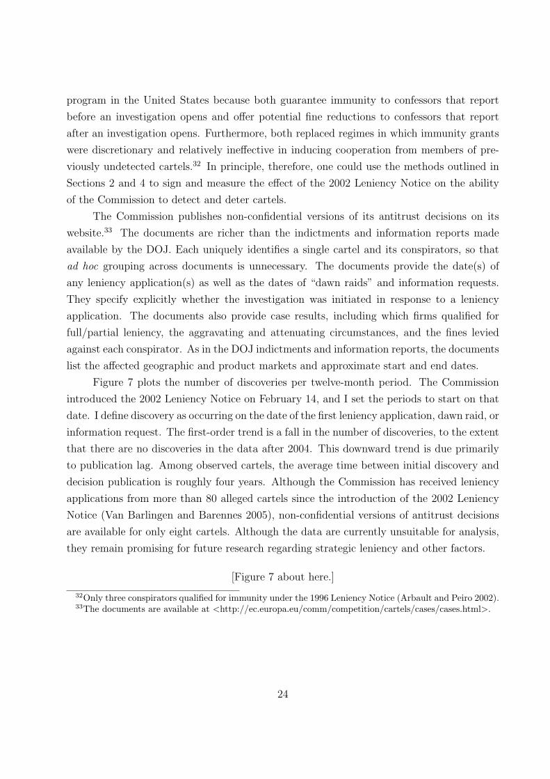
Figure 7 plots the number of discoveries per twelve-month period. The Commission

introduced the 2002 Leniency Notice on February 14, and I set the periods to start on that

date. I define discovery as occurring on the date of the first leniency application, dawn raid, or

information request. The first-order trend is a fall in the number of discoveries, to the extent

that there are no discoveries in the data after 2004. This downward trend is due primarily

to publication lag. Among observed cartels, the average time between initial discovery and

decision publication is roughly four years. Although the Commission has received leniency

applications from more than 80 alleged cartels since the introduction of the 2002 Leniency

Notice (Van Barlingen and Barennes 2005), non-confidential versions of antitrust decisions

are available for only eight cartels. Although the data are currently unsuitable for analysis,

they remain promising for future research regarding strategic leniency and other factors.

[Figure 7 about here.]

32Only three conspirators qualified for immunity under the 1996 Leniency Notice (Arbault and Peiro 2002).33The documents are available at <http://ec.europa.eu/comm/competition/cartels/cases/cases.html>.

24

7 Conclusion

Antitrust authorities in the U.S. and elsewhere guarantee early cartel confessors full amnesty

from state prosecution. The game-theoretical literature is ambiguous regarding the impacts

of this leniency. In this paper, I provide empirical evidence regarding the efficacy of leniency

based on the experience in the United States. I develop a theoretical model of cartel behavior

that provides empirical predictions and moment conditions, and apply the model to the

complete set of indictments and information reports issued by the DOJ over a twenty-year

span. Reduced form statistical tests are consistent with the notion that leniency enhances

deterrence and detection capabilities. Direct estimation of the model, via the method of

moments, yields a 59 percent lower cartel formation rate and a 62 percent higher cartel

detection rate due to leniency.

References

[1] Arbault, Francois and Francisco Peiro. 2002. The Commission’s new notice on immu-nity and reductiuon of fines in cartel cases: building on success. Competition PolicyNewsletter, 2: 15-22.

[2] Aubert, Cecile, Patrick Rey, and William E. Kovacic. 2006. The impact of leniency andwhistle-blowing programs on cartels. International Journal of Industrial Organization,24: 1241-1266.

[3] Bingaman, Anne K. 1994. “Report from the Antitrust Division, Spring 1994.” Availablefor download at <http://www.usdoj.gov/atr/public/speeches/0110.htm>.

[4] Breusch, T.S. 1978. Testing for autocorrelation in dynamic linear models. AustralianEconomic Papers, 17(31): 334-355.

[5] Brenner, Steffan. 2005. “An empirical study of the European corporate leniency pro-gram.” Manuscript, Humboldt-University Berlin.

[6] Bryant, Peter G. and E. Woodrow Eckard. 1991. Price fixing: the probability of gettingcaught. Review of Economonics and Statistics, 73: 531-536.

[7] Casella, George and Roger L. Berger. 2002. Statistical Inference, 2nd ed. Duxbury,Pacific Grove, CA.

[8] Chen, Joe and Joseph E. Harrington, Jr. 2007. The impact of the corporate leniency pro-gram on cartel formation and the cartel price path. The Political Economy of Antitrust,Vivek Ghosal and Johan Stennek, eds., Elsevier.

25

[9] Connor, John M. 2001. “Our customers are our enemies”: the lysine cartel of 1992-1995.Review of Industrial Organization, 18: 5-21.

[10] Connor, John M. 2004. Price-fixing overcharges: legal and economic evidence. StaffPaper 04-17. Department of Agricultural Economics, Purdue University.

[11] Connor, John M., and Yuliya Bolotova. 2005. “Cartel overcharges: survey and meta-analysis.” Manuscript, Purdue University.

[12] Ellis, Christopher J. and Wesley W. Wilson. 2003. “Cartels, price-fixing, and corporateleniency policy: what doesn’t kill us makes us stronger.” Manuscript, University ofOregon.

[13] Froeb, Luke M., Robert A. Koyak, and Gregory J. Werden. 1993. What is the effect ofbid-rigging on prices? Economic Letters, 42: 419-423.

[14] Ghosal, Vivek and Joseph Gallo. 2001. The cyclical behavior of the Department of Jus-tice’s antitrust enforcement activity. International Journal of Industrial Organization,19, 27-54.

[15] Ghosal, Vivek. 2004. “Regime shifts in antitrust.” Manuscript, Georgia Institute ofTechnology.

[16] Godfrey, Leslie G. 1978. Testing for higher order serial correlation in regression equationswhen the regressors include lagged dependent variables. Econometrica, 46(6), 1303-1310.

[17] Greene, William H. (2003). Econometric Analysis, 5th ed. Prentice-Hall, Upper SaddleRiver, NJ.

[18] Hammond, Scott D. 2000. “Fighting cartels – why and how? Lessons com-mon to detecting and deterring cartel activity.” Available for download at<http://www.usdoj.gov/atr/public/speeches/6487.htm>.

[19] Hammond, Scott D. 2001. “When calculating the costs and benefits of applying forcorporate amnesty, how do you put a price tag on an individual’s freedom?” Availablefor download at <http://www.usdoj.gov/atr/public/speeches/7647.htm>.

[20] Hammond, Scott D. 2004. “Cornerstones of an effective leniency policy.” Available fordownload at <http://www.usdoj.gov/atr/public/speeches/206611.htm>.

[21] Hammond, Scott D. 2005. “An update of the Antitrust Divi-sion’s criminal enforcement program. Available for download at<http://www.usdoj.gov/atr/public/speeches/213247.htm>

[22] Hansen, Lars P. 1982. Large sample properties of generalized method of moments esti-mators. Econometrica, 50: 1029-1054.

26

[23] Harrington, Joseph E., Jr. Forthcoming. “Optimal corporate leniency programs.” Jour-nal of Industrial Economics.

[24] Harrington, Joseph E., and Myong-Hun Chang. 2007. Modelling the birth and death ofcartels with an application to evaluating antitrust policy. Mimeo.

[25] Hinloopen, Jeroen. 2003. An economic analysis of leniency programs in antitrust law.De Economist 151(4): 415-432.

[26] Howard, Jeffery H. and David Kaserman. 1989. Proof of damages in construction bidrigging cases. The Antitrust Bulletin, 34: 359-393.

[27] Kwoka, John E., Jr. 1997. The price effects of bidding conspiracies: evidence from realestate auctions. The Antitrust Bulletin, 42: 503-516.

[28] Motchenkova, Evguenia. 2004. “The effects of leniency programs on the behavior offirms participating in cartel agreements.” Manuscript, Tillburg University.

[29] Motchenkova, Evguenia and van der Lann. 2005. “Strictness of leniency programs andcartels of asymmetric firms.” CentER Discussion Paper 74, Tillburg University.

[30] Motta, Massimo and Michele Polo. 2003. Leniency programs and cartel prosecution.International Journal of Industrial Organization, 21: 347-379.

[31] Newey, Whitney K. and Kenneth D. West. 1987. A simple positive semi-definite, het-eroskedasticity and autocorrelation consistent covariance matrix. Econometrica, 55, 703-708.

[32] O.E.C.D. Fighting Hard Core Cartels: Harm, Effective Sanctions and Leniency Pro-grammes, 2002, Paris.

[33] O.E.C.D. Hard Core Cartels. Recent Progress and Challenges Ahead, 2003, Paris.

[34] Pate, R. Hewitt. 2004. “International anti-cartel enforcement.” Available for downloadat <http://www.usdoj.gov/atr/public/speeches/206428.htm>.

[35] Porter, Robert H., and J. Douglas Zona. 1993. Ohio school milk markets: an analysisof bidding. RAND Journal of Economics. 30: 263-288.

[36] Rey, Patrick. 2003. Towards a theory of competition policy. Advances in Economicsand Econometrics: Theory and Applications, M. Dewatripont, L.P. Hansen, and S.J.Turnovsky eds., Cambridge University Press.

[37] Ruud, Paul A. 2000. An Introduction to Classical Econometric Theory. Oxford Univer-sity Press, New York, NY.

[38] Spagnolo, Giancarlo. 2000. “Optimal leniency programs.” F.E.E.M. Nota di Lavoro No.42.00, Fondazione ENI “Enrico Mattei,” Milano.

27

[39] Spagnolo, Giancarlo. 2004. “Divide et impera: Optimal deterrence mechanisms againstcartels (and organized crime).” Manuscript, University of Mannheim.

[40] Spagnolo, Giancarlo. 2006. “Leniency and whistleblowers in antitrust.” CEPR Discus-sion Paper No. 5794.

[41] Spratling, Gary R. 1998. “The corporate leniency policy: an-swers to recurring questions.” Available for download at<http://www.usdoj.gov/atr/public/speeches/1626.htm>.

[42] Spratling, Gary R. 1999 “Making companies an offer they shouldn’t refuse.” Availablefor download at <http://www.usdoj.gov/atr/public/speeches/2247.htm>.

[43] U.S. Sentencing Committee. Sourcebook of Federal Sentencing Statistics, 10, 2005.

[44] Van Barlingen, Bertus. 2003. The European Commission’s leniency notice after one yearof operation. Competition Policy Newsletter, 2: 16-21.

[45] Van Barlingen, Bertus and Marc Barennes. 2005. The European Commission’s 2002leniency notice in practice. Competition Policy Newsletter, 3: 6-16.

[46] Whinston, Michael D. 2006. Lectures on Antitrust Economics. The MIT Press, Cam-bridge, Massachusetts.

[47] White, Lawrence J. 2001. Lysine and price fixing: How long? How severe? Review ofIndustrial Organization, 18: 23-31.

APPENDICES

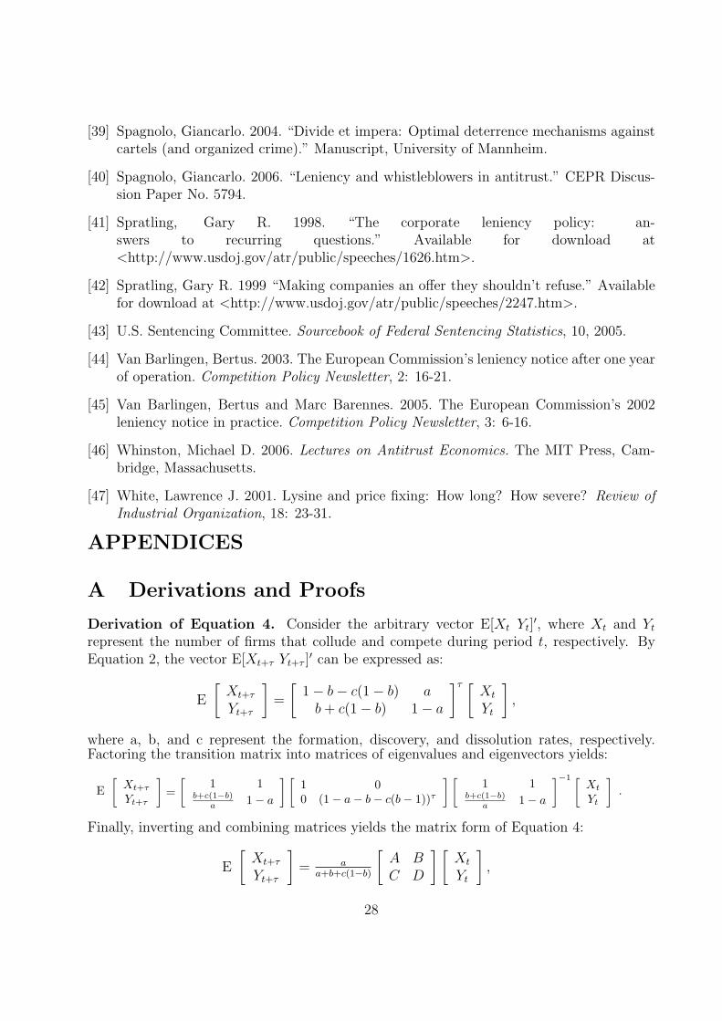
A Derivations and Proofs

Derivation of Equation 4. Consider the arbitrary vector E[Xt Yt]′, where Xt and Yt

represent the number of firms that collude and compete during period t, respectively. ByEquation 2, the vector E[Xt+τ Yt+τ ]

′ can be expressed as:

E

[Xt+τ

Yt+τ

]=

[1− b− c(1− b) a

b + c(1− b) 1− a

]τ [Xt

Yt

],

where a, b, and c represent the formation, discovery, and dissolution rates, respectively.Factoring the transition matrix into matrices of eigenvalues and eigenvectors yields:

E[

Xt+τ

Yt+τ

]=

[1 1

b+c(1−b)a 1− a

] [1 00 (1− a− b− c(b− 1))τ

] [1 1

b+c(1−b)a 1− a

]−1 [Xt

Yt

].

Finally, inverting and combining matrices yields the matrix form of Equation 4:

E

[Xt+τ

Yt+τ

]= a

a+b+c(1−b)

[A BC D

] [Xt

Yt

],

28

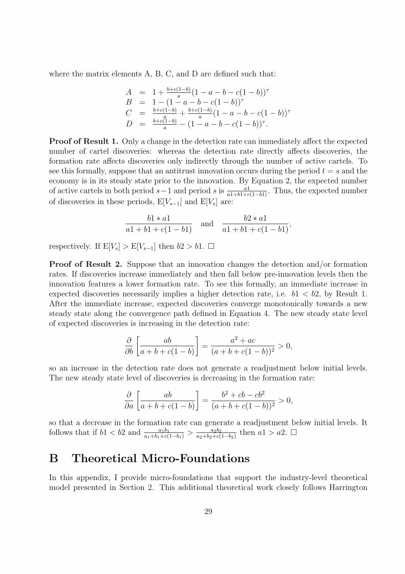
where the matrix elements A, B, C, and D are defined such that:

A = 1 + b+c(1−b)a

(1− a− b− c(1− b))τ

B = 1− (1− a− b− c(1− b))τ

C = b+c(1−b)a

+ b+c(1−b)a

(1− a− b− c(1− b))τ

D = b+c(1−b)a

− (1− a− b− c(1− b))τ .

Proof of Result 1. Only a change in the detection rate can immediately affect the expectednumber of cartel discoveries: whereas the detection rate directly affects discoveries, theformation rate affects discoveries only indirectly through the number of active cartels. Tosee this formally, suppose that an antitrust innovation occurs during the period t = s and theeconomy is in its steady state prior to the innovation. By Equation 2, the expected numberof active cartels in both period s−1 and period s is a1

a1+b1+c(1−b1). Thus, the expected number

of discoveries in these periods, E[Vs−1] and E[Vs] are:

b1 ∗ a1

a1 + b1 + c(1− b1)and

b2 ∗ a1

a1 + b1 + c(1− b1),

respectively. If E[Vs] > E[Vs−1] then b2 > b1. ¤

Proof of Result 2. Suppose that an innovation changes the detection and/or formationrates. If discoveries increase immediately and then fall below pre-innovation levels then theinnovation features a lower formation rate. To see this formally, an immediate increase inexpected discoveries necessarily implies a higher detection rate, i.e. b1 < b2, by Result 1.After the immediate increase, expected discoveries converge monotonically towards a newsteady state along the convergence path defined in Equation 4. The new steady state levelof expected discoveries is increasing in the detection rate:

∂

∂b

[ab

a + b + c(1− b)

]=

a2 + ac

(a + b + c(1− b))2> 0,

so an increase in the detection rate does not generate a readjustment below initial levels.The new steady state level of discoveries is decreasing in the formation rate:

∂

∂a

[ab

a + b + c(1− b)

]=

b2 + cb− cb2

(a + b + c(1− b))2> 0,

so that a decrease in the formation rate can generate a readjustment below initial levels. Itfollows that if b1 < b2 and a1b1

a1+b1+c(1−b1)> a2b2

a2+b2+c(1−b2)then a1 > a2. ¤

B Theoretical Micro-Foundations

In this appendix, I provide micro-foundations that support the industry-level theoreticalmodel presented in Section 2. This additional theoretical work closely follows Harrington

29

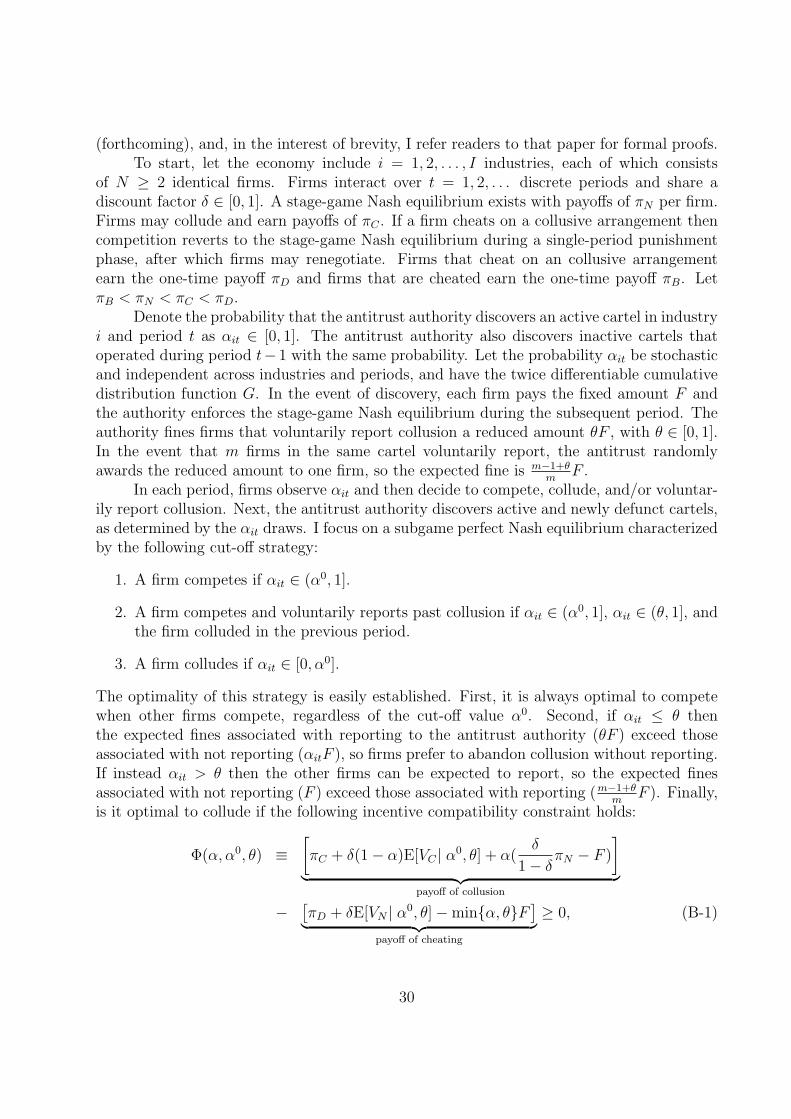
(forthcoming), and, in the interest of brevity, I refer readers to that paper for formal proofs.To start, let the economy include i = 1, 2, . . . , I industries, each of which consists

of N ≥ 2 identical firms. Firms interact over t = 1, 2, . . . discrete periods and share adiscount factor δ ∈ [0, 1]. A stage-game Nash equilibrium exists with payoffs of πN per firm.Firms may collude and earn payoffs of πC . If a firm cheats on a collusive arrangement thencompetition reverts to the stage-game Nash equilibrium during a single-period punishmentphase, after which firms may renegotiate. Firms that cheat on an collusive arrangementearn the one-time payoff πD and firms that are cheated earn the one-time payoff πB. LetπB < πN < πC < πD.

Denote the probability that the antitrust authority discovers an active cartel in industryi and period t as αit ∈ [0, 1]. The antitrust authority also discovers inactive cartels thatoperated during period t−1 with the same probability. Let the probability αit be stochasticand independent across industries and periods, and have the twice differentiable cumulativedistribution function G. In the event of discovery, each firm pays the fixed amount F andthe authority enforces the stage-game Nash equilibrium during the subsequent period. Theauthority fines firms that voluntarily report collusion a reduced amount θF , with θ ∈ [0, 1].In the event that m firms in the same cartel voluntarily report, the antitrust randomlyawards the reduced amount to one firm, so the expected fine is m−1+θ

mF .

In each period, firms observe αit and then decide to compete, collude, and/or voluntar-ily report collusion. Next, the antitrust authority discovers active and newly defunct cartels,as determined by the αit draws. I focus on a subgame perfect Nash equilibrium characterizedby the following cut-off strategy:

1. A firm competes if αit ∈ (α0, 1].

2. A firm competes and voluntarily reports past collusion if αit ∈ (α0, 1], αit ∈ (θ, 1], andthe firm colluded in the previous period.

3. A firm colludes if αit ∈ [0, α0].

The optimality of this strategy is easily established. First, it is always optimal to competewhen other firms compete, regardless of the cut-off value α0. Second, if αit ≤ θ thenthe expected fines associated with reporting to the antitrust authority (θF ) exceed thoseassociated with not reporting (αitF ), so firms prefer to abandon collusion without reporting.If instead αit > θ then the other firms can be expected to report, so the expected finesassociated with not reporting (F ) exceed those associated with reporting (m−1+θ

mF ). Finally,

is it optimal to collude if the following incentive compatibility constraint holds:

Φ(α, α0, θ) ≡[πC + δ(1− α)E[VC | α0, θ] + α(

δ

1− δπN − F )

]

︸ ︷︷ ︸payoff of collusion

− [πD + δE[VN | α0, θ]−minα, θF ]

︸ ︷︷ ︸payoff of cheating

≥ 0, (B-1)

30

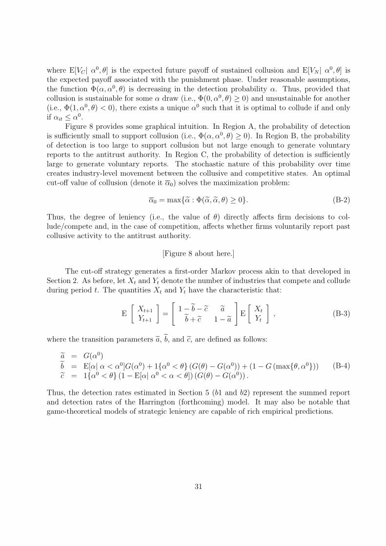
where E[VC | α0, θ] is the expected future payoff of sustained collusion and E[VN | α0, θ] isthe expected payoff associated with the punishment phase. Under reasonable assumptions,the function Φ(α, α0, θ) is decreasing in the detection probability α. Thus, provided thatcollusion is sustainable for some α draw (i.e., Φ(0, α0, θ) ≥ 0) and unsustainable for another(i.e., Φ(1, α0, θ) < 0), there exists a unique α0 such that it is optimal to collude if and onlyif αit ≤ α0.

Figure 8 provides some graphical intuition. In Region A, the probability of detectionis sufficiently small to support collusion (i.e., Φ(α, α0, θ) ≥ 0). In Region B, the probabilityof detection is too large to support collusion but not large enough to generate voluntaryreports to the antitrust authority. In Region C, the probability of detection is sufficientlylarge to generate voluntary reports. The stochastic nature of this probability over timecreates industry-level movement between the collusive and competitive states. An optimalcut-off value of collusion (denote it α0) solves the maximization problem:

α0 = maxα : Φ(α, α, θ) ≥ 0. (B-2)

Thus, the degree of leniency (i.e., the value of θ) directly affects firm decisions to col-lude/compete and, in the case of competition, affects whether firms voluntarily report pastcollusive activity to the antitrust authority.

[Figure 8 about here.]

The cut-off strategy generates a first-order Markov process akin to that developed inSection 2. As before, let Xt and Yt denote the number of industries that compete and colludeduring period t. The quantities Xt and Yt have the characteristic that:

E

[Xt+1

Yt+1

]=

[1− b− c a

b + c 1− a

]E

[Xt

Yt

], (B-3)

where the transition parameters a, b, and c, are defined as follows:

a = G(α0)

b = E[α| α < α0]G(α0) + 1α0 < θ (G(θ)−G(α0)) + (1−G (maxθ, α0))c = 1α0 < θ (1− E[α| α0 < α < θ]) (G(θ)−G(α0)) .

(B-4)

Thus, the detection rates estimated in Section 5 (b1 and b2) represent the summed reportand detection rates of the Harrington (forthcoming) model. It may also be notable thatgame-theoretical models of strategic leniency are capable of rich empirical predictions.

31

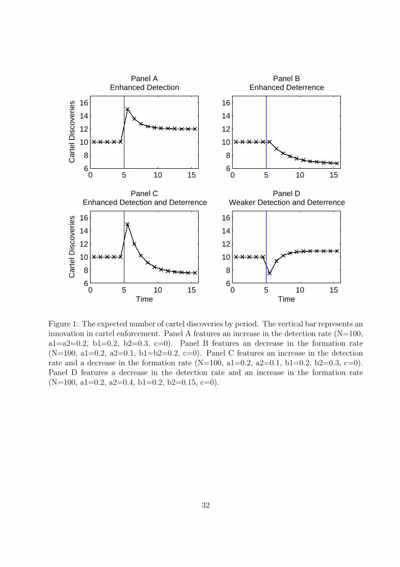
0 5 10 156

8

10

12

14

16

Car

tel D

isco

verie

sPanel A

Enhanced Detection

0 5 10 156

8

10

12

14

16

Panel BEnhanced Deterrence

0 5 10 156

8

10

12

14

16

Time

Car

tel D

isco

verie

s

Panel CEnhanced Detection and Deterrence

0 5 10 156

8

10

12

14

16

Time

Panel DWeaker Detection and Deterrence

Figure 1: The expected number of cartel discoveries by period. The vertical bar represents aninnovation in cartel enforcement. Panel A features an increase in the detection rate (N=100,a1=a2=0.2, b1=0.2, b2=0.3, c=0). Panel B features an decrease in the formation rate(N=100, a1=0.2, a2=0.1, b1=b2=0.2, c=0). Panel C features an increase in the detectionrate and a decrease in the formation rate (N=100, a1=0.2, a2=0.1, b1=0.2, b2=0.3, c=0).Panel D features a decrease in the detection rate and an increase in the formation rate(N=100, a1=0.2, a2=0.4, b1=0.2, b2=0.15, c=0).

32

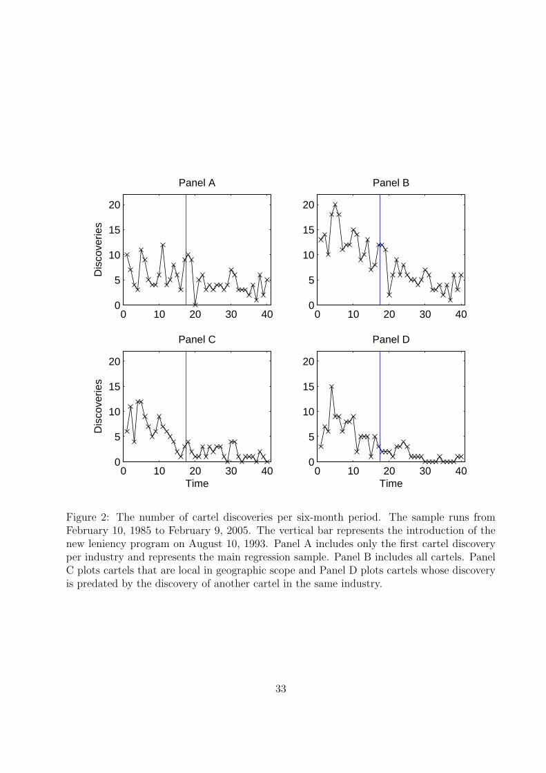
0 10 20 30 400

5

10

15

20

Dis

cove

ries

Panel A

0 10 20 30 400

5

10

15

20

Panel B

0 10 20 30 400

5

10

15

20

Time

Dis

cove

ries

Panel C

0 10 20 30 400

5

10

15

20

Time

Panel D

Figure 2: The number of cartel discoveries per six-month period. The sample runs fromFebruary 10, 1985 to February 9, 2005. The vertical bar represents the introduction of thenew leniency program on August 10, 1993. Panel A includes only the first cartel discoveryper industry and represents the main regression sample. Panel B includes all cartels. PanelC plots cartels that are local in geographic scope and Panel D plots cartels whose discoveryis predated by the discovery of another cartel in the same industry.

33

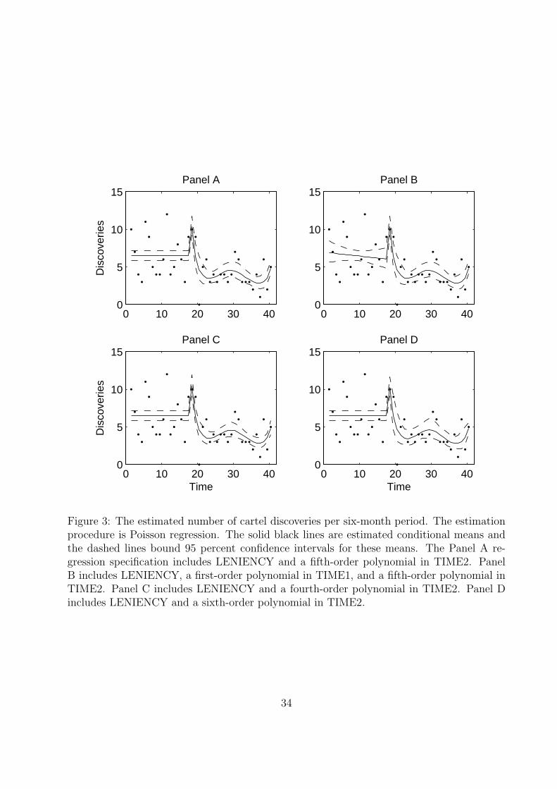
0 10 20 30 400

5

10

15

Dis

cove

ries

Panel A

0 10 20 30 400

5

10

15Panel B

0 10 20 30 400

5

10

15

Time

Dis

cove

ries

Panel C

0 10 20 30 400

5

10

15

Time

Panel D

Figure 3: The estimated number of cartel discoveries per six-month period. The estimationprocedure is Poisson regression. The solid black lines are estimated conditional means andthe dashed lines bound 95 percent confidence intervals for these means. The Panel A re-gression specification includes LENIENCY and a fifth-order polynomial in TIME2. PanelB includes LENIENCY, a first-order polynomial in TIME1, and a fifth-order polynomial inTIME2. Panel C includes LENIENCY and a fourth-order polynomial in TIME2. Panel Dincludes LENIENCY and a sixth-order polynomial in TIME2.

34

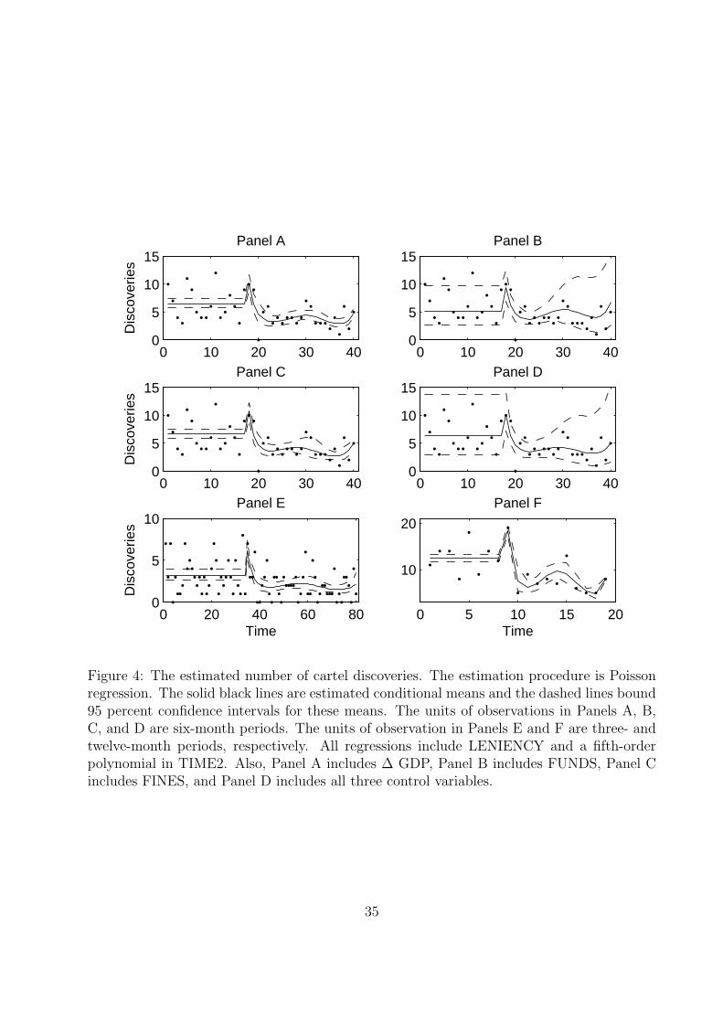
0 10 20 30 400

5

10

15

Dis

cove

ries

Panel A

0 10 20 30 400

5

10

15Panel B

0 10 20 30 400

5

10

15

Dis

cove

ries

Panel C

0 10 20 30 400

5

10

15Panel D

0 20 40 60 800

5

10

Time

Dis

cove

ries

Panel E

0 5 10 15 20

10

20

Time

Panel F

Figure 4: The estimated number of cartel discoveries. The estimation procedure is Poissonregression. The solid black lines are estimated conditional means and the dashed lines bound95 percent confidence intervals for these means. The units of observations in Panels A, B,C, and D are six-month periods. The units of observation in Panels E and F are three- andtwelve-month periods, respectively. All regressions include LENIENCY and a fifth-orderpolynomial in TIME2. Also, Panel A includes ∆ GDP, Panel B includes FUNDS, Panel Cincludes FINES, and Panel D includes all three control variables.

35

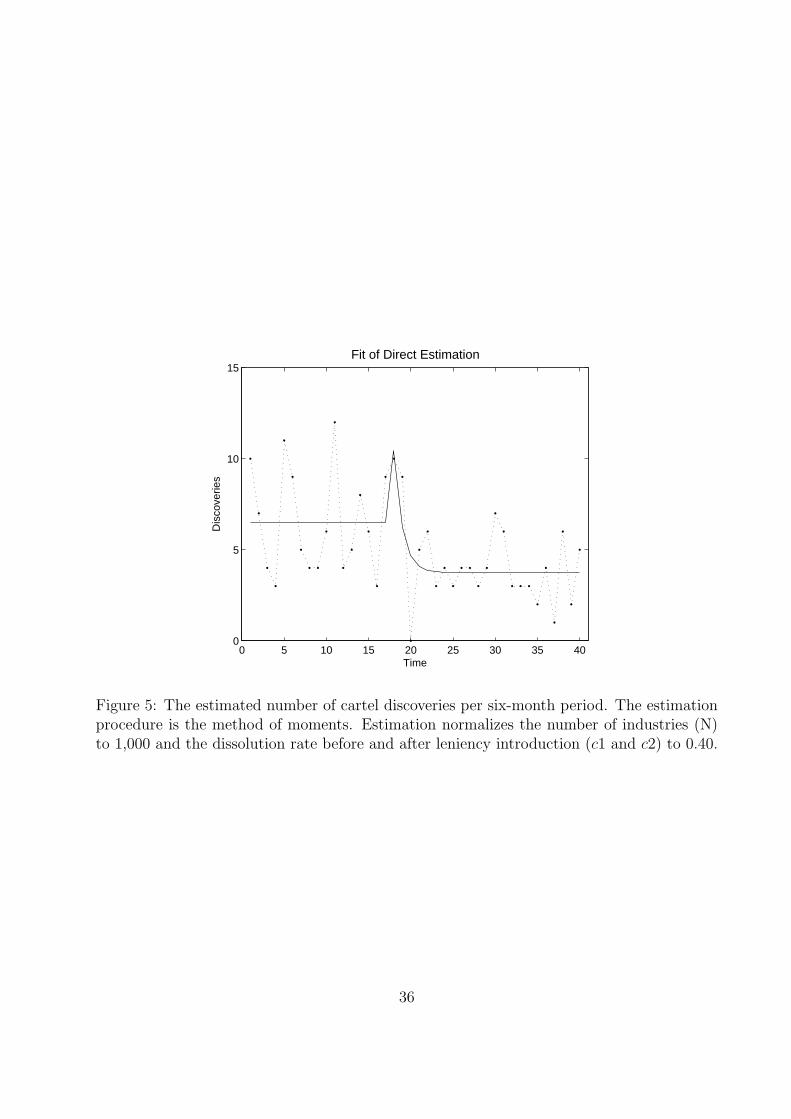
0 5 10 15 20 25 30 35 400

5

10

15

Time

Dis

cove

ries

Fit of Direct Estimation

Figure 5: The estimated number of cartel discoveries per six-month period. The estimationprocedure is the method of moments. Estimation normalizes the number of industries (N)to 1,000 and the dissolution rate before and after leniency introduction (c1 and c2) to 0.40.

36

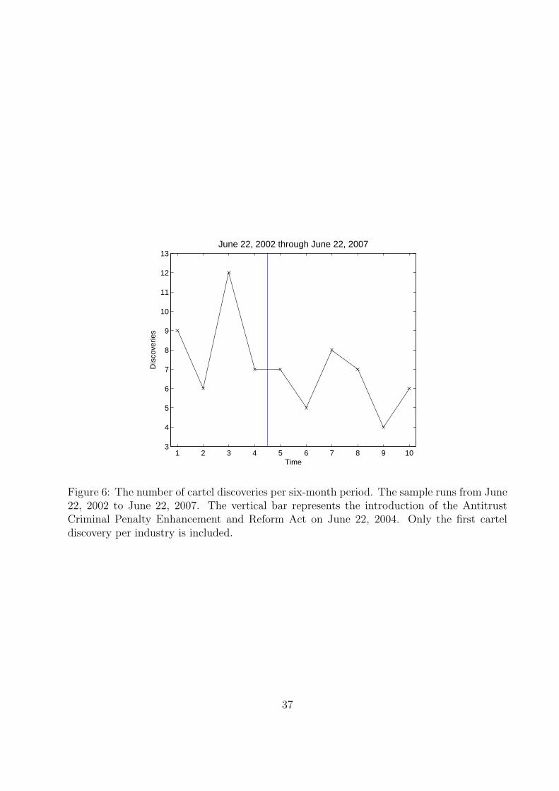
1 2 3 4 5 6 7 8 9 103

4

5

6

7

8

9

10

11

12

13

Dis

cove

ries

Time

June 22, 2002 through June 22, 2007

Figure 6: The number of cartel discoveries per six-month period. The sample runs from June22, 2002 to June 22, 2007. The vertical bar represents the introduction of the AntitrustCriminal Penalty Enhancement and Reform Act on June 22, 2004. Only the first carteldiscovery per industry is included.

37

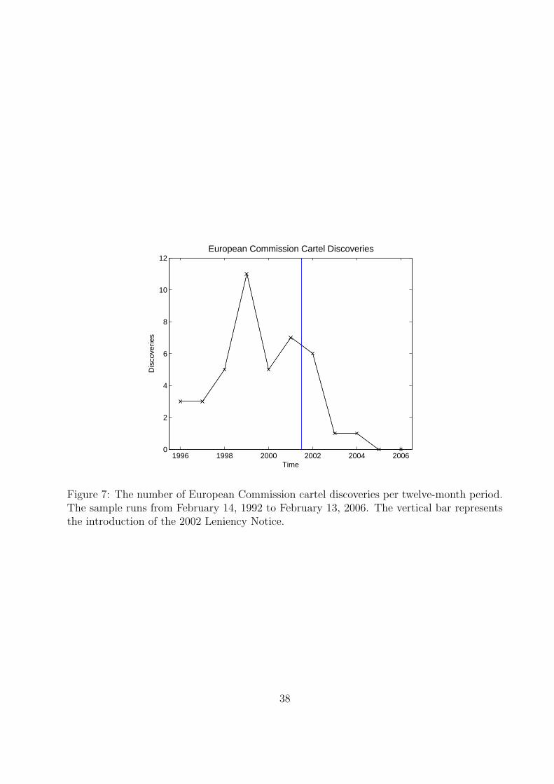
1996 1998 2000 2002 2004 20060

2

4

6

8

10

12

Time

Dis

cove

ries

European Commission Cartel Discoveries

Figure 7: The number of European Commission cartel discoveries per twelve-month period.The sample runs from February 14, 1992 to February 13, 2006. The vertical bar representsthe introduction of the 2002 Leniency Notice.

38

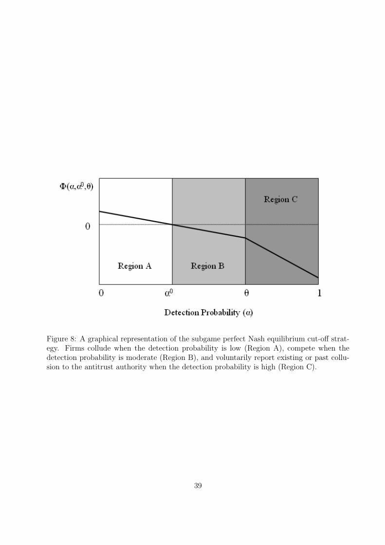
Figure 8: A graphical representation of the subgame perfect Nash equilibrium cut-off strat-egy. Firms collude when the detection probability is low (Region A), compete when thedetection probability is moderate (Region B), and voluntarily report existing or past collu-sion to the antitrust authority when the detection probability is high (Region C).

39

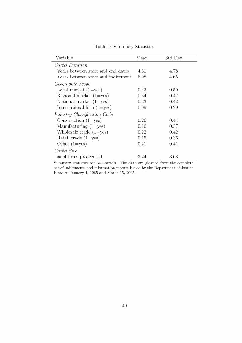
Table 1: Summary Statistics

Variable Mean Std Dev

Cartel DurationYears between start and end dates 4.61 4.78Years between start and indictment 6.98 4.65

Geographic ScopeLocal market (1=yes) 0.43 0.50Regional market (1=yes) 0.34 0.47National market (1=yes) 0.23 0.42International firm (1=yes) 0.09 0.29

Industry Classification CodeConstruction (1=yes) 0.26 0.44Manufacturing (1=yes) 0.16 0.37Wholesale trade (1=yes) 0.22 0.42Retail trade (1=yes) 0.15 0.36Other (1=yes) 0.21 0.41

Cartel Size# of firms prosecuted 3.24 3.68

Summary statistics for 343 cartels. The data are gleaned from the completeset of indictments and information reports issued by the Department of Justicebetween January 1, 1985 and March 15, 2005.

40

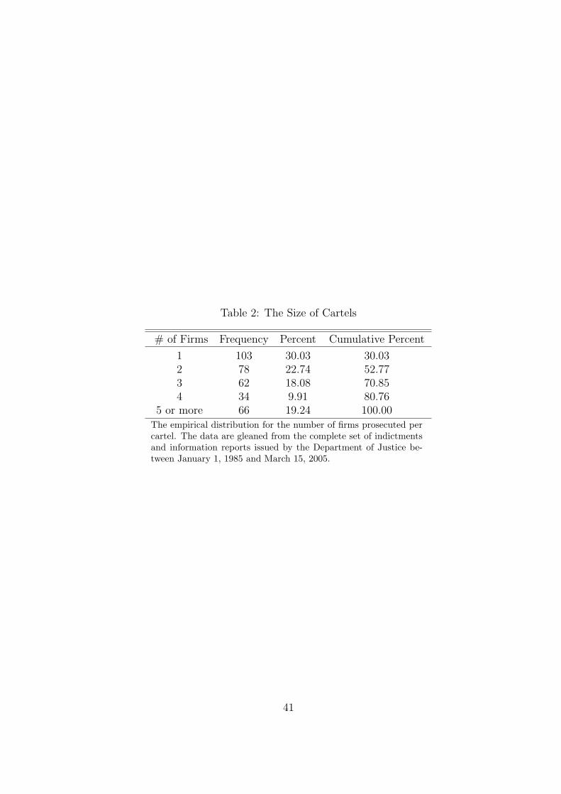
Table 2: The Size of Cartels

# of Firms Frequency Percent Cumulative Percent

1 103 30.03 30.032 78 22.74 52.773 62 18.08 70.854 34 9.91 80.76

5 or more 66 19.24 100.00The empirical distribution for the number of firms prosecuted percartel. The data are gleaned from the complete set of indictmentsand information reports issued by the Department of Justice be-tween January 1, 1985 and March 15, 2005.

41

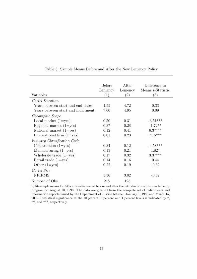
Table 3: Sample Means Before and After the New Leniency Policy

BeforeLeniency

AfterLeniency

Difference inMeans t-Statistic

Variables (1) (2) (3)

Cartel DurationYears between start and end dates 4.55 4.72 0.33Years between start and indictment 7.00 4.95 0.09

Geographic ScopeLocal market (1=yes) 0.50 0.31 -3.51***Regional market (1=yes) 0.37 0.28 -1.72**National market (1=yes) 0.12 0.41 6.37***International firm (1=yes) 0.01 0.23 7.15***

Industry Classification CodeConstruction (1=yes) 0.34 0.12 -4.58***Manufacturing (1=yes) 0.13 0.21 1.82*Wholesale trade (1=yes) 0.17 0.32 3.37***Retail trade (1=yes) 0.14 0.16 0.44Other (1=yes) 0.22 0.19 -0.62

Cartel SizeNFIRMS 3.36 3.02 -0.82

Number of Obs. 218 125Split-sample means for 343 cartels discovered before and after the introduction of the new leniencyprogram on August 10, 1993. The data are gleaned from the complete set of indictments andinformation reports issued by the Department of Justice between January 1, 1985 and March 15,2005. Statistical significance at the 10 percent, 5 percent and 1 percent levels is indicated by *,**, and ***, respectively.

42

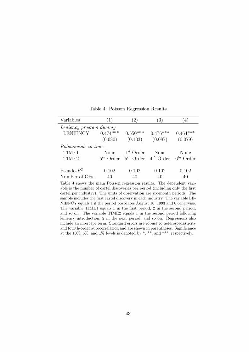
Table 4: Poisson Regression Results

Variables (1) (2) (3) (4)

Leniency program dummyLENIENCY 0.474*** 0.550*** 0.476*** 0.464***

(0.080) (0.133) (0.087) (0.079)

Polynomials in timeTIME1 None 1st Order None NoneTIME2 5th Order 5th Order 4th Order 6th Order

Pseudo-R2 0.102 0.102 0.102 0.102Number of Obs. 40 40 40 40Table 4 shows the main Poisson regression results. The dependent vari-able is the number of cartel discoveries per period (including only the firstcartel per industry). The units of observation are six-month periods. Thesample includes the first cartel discovery in each industry. The variable LE-NIENCY equals 1 if the period postdates August 10, 1993 and 0 otherwise.The variable TIME1 equals 1 in the first period, 2 in the second period,and so on. The variable TIME2 equals 1 in the second period followingleniency introduction, 2 in the next period, and so on. Regressions alsoinclude an intercept term. Standard errors are robust to heteroscedasticityand fourth-order autocorrelation and are shown in parentheses. Significanceat the 10%, 5%, and 1% levels is denoted by *, **, and ***, respectively.

43

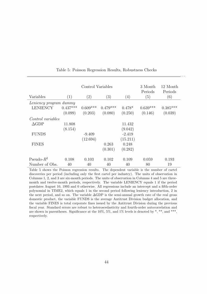
Table 5: Poisson Regression Results, Robustness Checks

Control Variables 3 MonthPeriods

12 MonthPeriods

Variables (1) (2) (3) (4) (5) (6)

Leniency program dummyLENIENCY 0.437*** 0.609*** 0.479*** 0.478* 0.639*** 0.385***

(0.099) (0.203) (0.080) (0.250) (0.146) (0.039)

Control variables∆GDP 11.808 11.432

(8.154) (9.042)FUNDS -9.409 -2.419

(12.694) (15.211)FINES 0.263 0.248

(0.301) (0.282)

Pseudo-R2 0.108 0.103 0.102 0.109 0.059 0.193Number of Obs. 40 40 40 40 80 19Table 5 shows the Poisson regression results. The dependent variable is the number of carteldiscoveries per period (including only the first cartel per industry). The units of observation inColumns 1, 2, and 3 are six-month periods. The units of observation in Columns 4 and 5 are three-month and twelve-month periods, respectively. The variable LENIENCY equals 1 if the periodpostdates August 10, 1993 and 0 otherwise. All regressions include an intercept and a fifth-orderpolynomial in TIME2, which equals 1 in the second period following leniency introduction, 2 inthe next period, and so on. The variable ∆GDP is the semi-annual growth rate of the real grossdomestic product, the variable FUNDS is the average Antitrust Division budget allocation, andthe variable FINES is total corporate fines issued by the Antitrust Division during the previousfiscal year. Standard errors are robust to heteroscedasticity and fourth-order autocorrelation andare shown in parentheses. Significance at the 10%, 5%, and 1% levels is denoted by *, **, and ***,respectively.

. . .

44

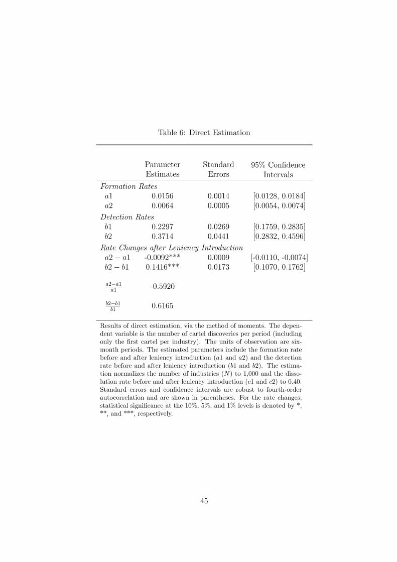
Table 6: Direct Estimation

ParameterEstimates

StandardErrors

95% ConfidenceIntervals

Formation Ratesa1 0.0156 0.0014 [0.0128, 0.0184]a2 0.0064 0.0005 [0.0054, 0.0074]

Detection Ratesb1 0.2297 0.0269 [0.1759, 0.2835]b2 0.3714 0.0441 [0.2832, 0.4596]

Rate Changes after Leniency Introductiona2− a1 -0.0092*** 0.0009 [-0.0110, -0.0074]b2− b1 0.1416*** 0.0173 [0.1070, 0.1762]

a2−a1a1

-0.5920

b2−b1b1

0.6165

Results of direct estimation, via the method of moments. The depen-dent variable is the number of cartel discoveries per period (includingonly the first cartel per industry). The units of observation are six-month periods. The estimated parameters include the formation ratebefore and after leniency introduction (a1 and a2) and the detectionrate before and after leniency introduction (b1 and b2). The estima-tion normalizes the number of industries (N) to 1,000 and the disso-lution rate before and after leniency introduction (c1 and c2) to 0.40.Standard errors and confidence intervals are robust to fourth-orderautocorrelation and are shown in parentheses. For the rate changes,statistical significance at the 10%, 5%, and 1% levels is denoted by *,**, and ***, respectively.

45

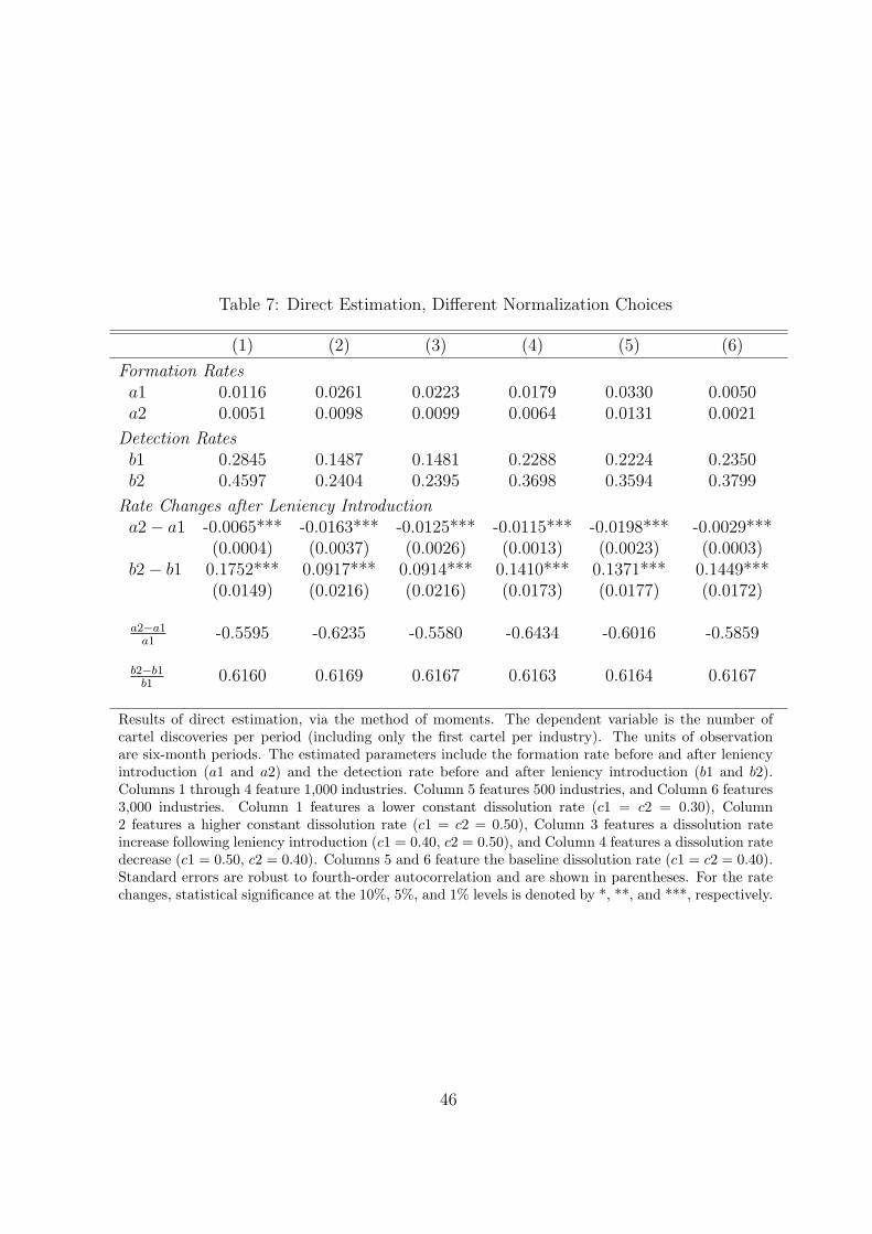
Table 7: Direct Estimation, Different Normalization Choices

(1) (2) (3) (4) (5) (6)

Formation Ratesa1 0.0116 0.0261 0.0223 0.0179 0.0330 0.0050a2 0.0051 0.0098 0.0099 0.0064 0.0131 0.0021

Detection Ratesb1 0.2845 0.1487 0.1481 0.2288 0.2224 0.2350b2 0.4597 0.2404 0.2395 0.3698 0.3594 0.3799

Rate Changes after Leniency Introductiona2− a1 -0.0065*** -0.0163*** -0.0125*** -0.0115*** -0.0198*** -0.0029***

(0.0004) (0.0037) (0.0026) (0.0013) (0.0023) (0.0003)b2− b1 0.1752*** 0.0917*** 0.0914*** 0.1410*** 0.1371*** 0.1449***

(0.0149) (0.0216) (0.0216) (0.0173) (0.0177) (0.0172)

a2−a1a1

-0.5595 -0.6235 -0.5580 -0.6434 -0.6016 -0.5859

b2−b1b1

0.6160 0.6169 0.6167 0.6163 0.6164 0.6167

Results of direct estimation, via the method of moments. The dependent variable is the number ofcartel discoveries per period (including only the first cartel per industry). The units of observationare six-month periods. The estimated parameters include the formation rate before and after leniencyintroduction (a1 and a2) and the detection rate before and after leniency introduction (b1 and b2).Columns 1 through 4 feature 1,000 industries. Column 5 features 500 industries, and Column 6 features3,000 industries. Column 1 features a lower constant dissolution rate (c1 = c2 = 0.30), Column2 features a higher constant dissolution rate (c1 = c2 = 0.50), Column 3 features a dissolution rateincrease following leniency introduction (c1 = 0.40, c2 = 0.50), and Column 4 features a dissolution ratedecrease (c1 = 0.50, c2 = 0.40). Columns 5 and 6 feature the baseline dissolution rate (c1 = c2 = 0.40).Standard errors are robust to fourth-order autocorrelation and are shown in parentheses. For the ratechanges, statistical significance at the 10%, 5%, and 1% levels is denoted by *, **, and ***, respectively.

46

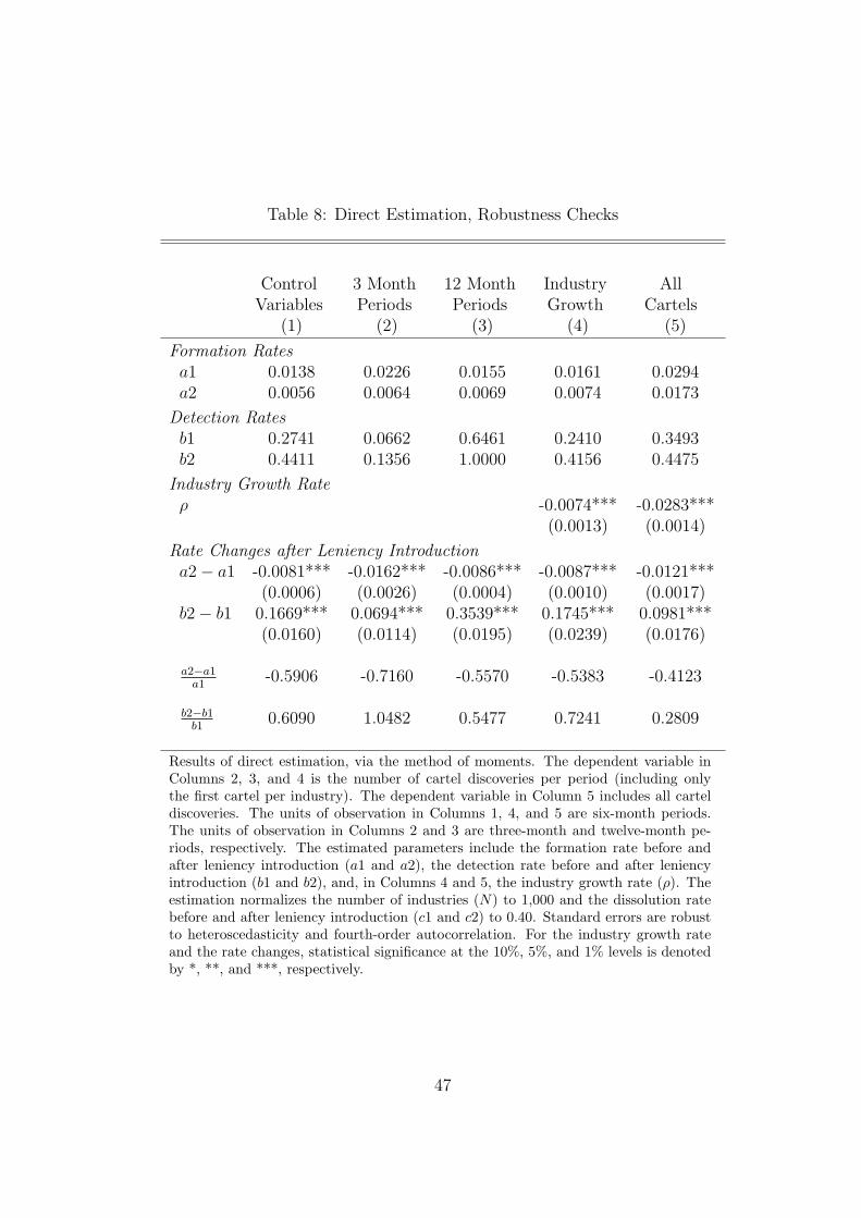
Table 8: Direct Estimation, Robustness Checks

ControlVariables

3 MonthPeriods

12 MonthPeriods

IndustryGrowth

AllCartels

(1) (2) (3) (4) (5)

Formation Ratesa1 0.0138 0.0226 0.0155 0.0161 0.0294a2 0.0056 0.0064 0.0069 0.0074 0.0173

Detection Ratesb1 0.2741 0.0662 0.6461 0.2410 0.3493b2 0.4411 0.1356 1.0000 0.4156 0.4475

Industry Growth Rateρ -0.0074*** -0.0283***

(0.0013) (0.0014)

Rate Changes after Leniency Introductiona2− a1 -0.0081*** -0.0162*** -0.0086*** -0.0087*** -0.0121***

(0.0006) (0.0026) (0.0004) (0.0010) (0.0017)b2− b1 0.1669*** 0.0694*** 0.3539*** 0.1745*** 0.0981***

(0.0160) (0.0114) (0.0195) (0.0239) (0.0176)

a2−a1a1

-0.5906 -0.7160 -0.5570 -0.5383 -0.4123

b2−b1b1

0.6090 1.0482 0.5477 0.7241 0.2809

Results of direct estimation, via the method of moments. The dependent variable inColumns 2, 3, and 4 is the number of cartel discoveries per period (including onlythe first cartel per industry). The dependent variable in Column 5 includes all carteldiscoveries. The units of observation in Columns 1, 4, and 5 are six-month periods.The units of observation in Columns 2 and 3 are three-month and twelve-month pe-riods, respectively. The estimated parameters include the formation rate before andafter leniency introduction (a1 and a2), the detection rate before and after leniencyintroduction (b1 and b2), and, in Columns 4 and 5, the industry growth rate (ρ). Theestimation normalizes the number of industries (N) to 1,000 and the dissolution ratebefore and after leniency introduction (c1 and c2) to 0.40. Standard errors are robustto heteroscedasticity and fourth-order autocorrelation. For the industry growth rateand the rate changes, statistical significance at the 10%, 5%, and 1% levels is denotedby *, **, and ***, respectively.

47