Strategic Impacts of Technology Switch-Over:

Who Benefits from Electronic Commerce?‡

Martin Bandulet∗

This version: March 2003∗∗

Abstract

The introduction of new digital production and distribution technologies

may alter the firms’ strategy sets, as they are not able to commit credibly

to quantity strategies anymore. Mixed oligopoly markets may emerge where

some companies compete in prices, while others adjust their quantities. Using

an approach first published by Reinhard Selten (1971) and developed further

by Richard Cornes and Roger Hartley (2001), I calculate the Nash equilibrium

of such an N -person game in a linear specification. Then I discuss the strategic

effect of a technology switch-over on market performance and social welfare.

A firm that introduces new technology suffers a srategic disadvantage, while

consumers benefit.

JEL–classification: D 43, L 13

Key words: Electronic Coordination, Oligopoly Theory, Product Differen-

tiation

‡This research has been supported by the Deutsche Forschungsgemeinschaft (DFG) within

the scope of the Forschergruppe “Effiziente elektronische Koordination in der Dienstleis-

tungswirtschaft” (FOR 275).∗Address: Martin Bandulet, Wirtschaftswissenschaftliche Fakultat, Universitat Augsburg, D–

86135 Augsburg, Deutschland, Tel. +49 (0821) 598-4197, Fax +49 (0821) 598-4230, E-mail:

Martin.Bandulet@Wiwi.Uni-Augsburg.DE∗∗First version: April 2002, Universitat Augsburg, Volkswirtschaftliche Diskussionsreihe, Beitrag

221.

1 Introduction

In recent years, a lot of research has been done to study the effects of emerging

electronic coordination in the field of production and distribution on the structure

and performance of oligopoly markets. Bakos (1997) discussed the consequences

of reduced search costs in electronic markets. Other related papers investigate the

impact of declining transport costs due to new technologies (see Morasch/Welzel,

2000), or the impact of changing cost structures as well as the increased potential

for product differentiation (see Belleflamme, 2001). The present paper is dedicated

to an aspect that has widely been neglected: The use of electronic coordination

in production technology may change players’ strategy sets and thus influence the

market result.

Consider the different causes for price and quantity competition that have widely

been discussed. In their seminal work, Kreps and Scheinkman (1983) describe the

influence of time structure on a firm’s strategy set in an oligopoly market: A player

can commit himself to a quantity strategy if he has to decide about his output before

sale or if the firm has to make sunk capacity investments before production. Under

these circumstances, the Cournot game can be interpreted as the reduced form of a

two-stage game where firms decide about capacity in the first stage and set prices in

the second. Guth (1995) extends this analysis by considering a heterogenous goods

market.

In a more general approach, Klemperer and Meyer (1989) assume that a company

can commit to a specific supply function whose slope follows from the production

technology the firm uses. As Vives (1999) elucidates, price and quantity setting be-

haviour can be interpreted as the extreme cases of a totally elastic or inelastic supply

function and arise from different slopes of marginal costs. While flat marginal costs

lead to Bertrand-like strategies, quantity strategies correspond to steep marginal

costs, linked to inflexible technologies.

Obviously, the latter case corresponds to old industry—e. g. steel-works—where

firms have to build huge plants before they start production. Still, similar constraints

also appear for modern industries and services. Records and CDs are pressed before

1

sale, thus producers have to decide on their circulation, first. Likewise, the network

of local agencies can be interpreted as a capacity constraint for insurance companies.

Banks face similar constraints, with regard to their branch offices. Besides, they are

bound to legal capital restrictions.

Yet, new electronic technologies have a strong impact on both production and distri-

bution of goods and services. Electronic commerce enables banks and insurance com-

panies to sell their services without making use of traditional distribution channels.

Internet banks buy services like emergency call centers on the market themselves,

whenever needed. Thus they can react flexibly on changing demand—outsourcing

enables them even to escape regulatory capital constraints (see Teske, 2002). More-

over, by using digital production it is no longer necessary to disseminate information

through physical media. As a consequence, the provider of information goods—that

is, publishers or music companies—may sell and distribute the plain information as

a download on-line.

Hence, the use of electronic coordination—especially to produce digital goods and

services—alters the production and distribution process in two important ways:

• Electronic coordination eliminates time lags between production and sale, as

flexible technologies allow firms to generate goods or services on demand.

• Capacity constraints vanish since new technologies enable (almost) unre-

stricted replication of information goods with marginal costs close to or at

zero level.

Following the reasoning above, suppliers that have already adopted such a new

technology are no longer in a position to commit themselves credibly to a quantity.

Instead of that, a move toward price-setting behaviour will take place. To capture

the essence of this move, I will assume that these firms behave as price competitors,

after they have adopted new technology. Other firms that still use old production

and distribution technology have to build up capacities before production. Thus,

they are assumed to set quantities.

2

Now consider a market where some firms have switched to new technologies, whereas

others still use old technology, that is, a market with both price and quantity setters.

Singh and Vives (1984) analyse a market like this in a duopoly framework, with one

price and quantity setter each. Sziderovsky and Molnar (1992) provide a more

general analysis of a so-called mixed oligopoly1 and prove existence and uniqueness

of the Nash equilibrium. However, their framework is not suitable to study the

consequences of a technology switch-over, since they do not provide explicite results.

The model I use is based on a framework with symmetrically differentiated products.

In its linear specification, it can be solved for the equilibrium by making use of recent

progress in the theory of aggregative games. This approach, introduced originally by

Reinhard Selten (1971) and developed further by Cornes and Hartley (2001), exploits

the special structure of games where the players’ payoff functions only depend on

two scalars—their own strategy and the unweighted sum of the choices made by

all players in the game, that is, the total aggressiveness of the game. Cornes and

Hartley (2001) also state that some games may be “k-reducable”, that is, players

decide not on one, but on k aggregable strategy variables. In fact, I apply that

extension here.

The paper is structured as follows. The next section presents the basic model. Pre-

suming profit maximation, replacement functions and collective response curves of

price or quantity setting firms will be derived to determine the Nash equilibrium of

the game. Section three continues with a comparative static analysis of the equilib-

rium. With regard to its effect on the firm’s strategy set, I discuss the implications

of a technology switch on a company’s own output, on its competitors and on mar-

ket efficiency. Implications for investment incentives are briefly discussed in the

conclusions.

1In another context, this expression is used to describe oligopoly markets with coexisting public

and private firms (see White, 1996).

3

2 The Basic Model

2.1 Model Assumptions and Strategic Demand

The basic model applies a concept of symmetric product differentiation originally

developed by Spence (1976) and Dixit and Stiglitz (1977). N firms2 (indexed by

i = 1, . . . , N) use a linear-homogenous technology creating individual and constant

marginal costs ci to produce a specific variety of a symmetrically differentiated

product xi sold at price pi. The demand functions for the firms’ products are

generated by a representative consumer with a linear-quadratic utility

u(x1, . . . , xN) =N∑

i=1

xi − 1

2

(N∑

i=1

x2i + b

N∑i=1

∑

i 6=j

xixj

)−

N∑i=1

pixi (1)

yielding inverse demand functions

pi = 1− xi − b∑

j 6=i

xj. (2)

The parameter b measures the degree of substitutability between any two products.

If b = 1, products are perfect substitutes, whereas all firms produce independent

goods if b = 0.

Suppose that in a simultanous move n companies (i = 1, . . . , n) play Cournot strate-

gies (that is, set quantities), while N−n firms (i = n+1, . . . , N) play price strategies.

Seperating exogenous (strategically chosen) and endogenous prices and quantities

results in the following inverse demand for a quantity adjusting firm j and a price

setting firm k, respectively:

pj = 1− b

n∑

i=1,i 6=j

xi − b

N∑i=n+1

xi − xj

= 1− b

n∑i=1

xi − b

N∑i=n+1

xi − (1− b)xj (3)

2I assume that all firms earn positive profits and actually participate in the market. However,

an endogenous market entry decision that may be added in a two stage model would not change

any basic results.

4

pk = 1− b

n∑i=1

xi − b

N∑

i=n+1,i 6=k

xi − xk

= 1− b

n∑i=1

xi − b

N∑i=n+1

xi − (1− b)xk (4)

Equation (4) can be transformed into a direct demand function:

xk =1− b

∑ni=1 xi − b

∑Ni=n+1 xi − pk

1− b(5)

Summing up the (N − n) demand functions of the firms using price strategies and

rearranging terms, gives the total quantity produced by the Bertrand players:

N∑i=n+1

xi =(N − n)(1− b

∑ni=1 xi)−

∑Ni=n+1 pi

1 + b(N − n− 1)(6)

After inserting this expression into (3) and (5) and denoting the aggregate of strate-

gic price and quantity choices∑N

i=n+1 pi and∑n

i=1 xi by P and X, respectively, the

(inverse) demand functions can be written in their strategic form

pj =1− b

1 + b(N − n− 1)− (1− b)xj − b(1− b)X

1 + b(N − n− 1)

+bP

1 + b(N − n− 1)(7)

xk =1

1 + b(N − n− 1)− pk

1− b− bX

1 + b(N − n− 1)

+bP

(1 + b(N − n− 1))(1− b)(8)

Equations (3) and (5) are now available in a form, such that the strategically chosen

(exogenous) sizes appear on the right hand side, whereas endogenous variables can

be found on the left hand side. Now the aggregative character of the game becomes

obvious: Both endogenous output of the Bertrand players and the prices of the

Cournot firms—and thus profits—only depend on their own strategy (that is, their

aggressiveness) and the total sum of strategically chosen prices and quantities. Ac-

cording to Cornes and Hartley (2001), a game of this structure is “two-reducable”,

that is, it can be reduced into a system of two equations and then be solved for the

Nash equilibrium.

5

2.2 Collective Response and the Mixed-Oligopoly Nash

Equilibrium

Consider now the Cournot and Bertrand players maximizing their profits:

maxxj

πj(xj,P,X) = pj(xj,P,X) · xj − cj · xj (9)

maxpk

πk(pk,P,X) = pk · xk(pk,P,X)− ck · xk(pk,P,X) (10)

Firm j seeks to maximize its profit by choosing quantity xj, taking as given the

aggregate quantity produced by its competitors, X − xj, as well as the sum of

all strategic prices P. In contrast, a firm k considers the effect of its own price

decision on aggregate P, given a fixed X and fixed aggregate prices of its Bertrand

competitors, P− pk. Solving for the first order conditions, one receives firm j’s and

firm k’s so-called replacement function ηi(X,P):3

xj = ηj(X,P) =1− b− b(1− b)X + bP− (1− b + b(N − n))cj

(1− b)(2− b + 2b(N − n))(11)

pk = ηk(X,P) =1− b− b(1− b)X + bP + (1− 2b + b(N − n))ck

2− 3b + 2b(N − n)(12)

Unlike a reaction function, ηi does not describe a player i’s optimal response to his

competitors’ strategy choice (that is, X − xj or P − pk, respectively), but to the

total aggregate X or P, which includes his own strategy choice.4 Using the fact that

in equilibrium the aggregate reaction complies with the aggregate strategy choice—

so∑n

i=1 ηj(X,P) = X and∑N

i=n+1 ηk(X,P) = P—we can solve for the strategic

quantity produced and the strategic price aggregate, that is,

X =(1− b)n + bnP− (1− b + b(N − n))

∑ni=1 ci

(1− b)(2− b + b(2N − n))(13)

P =(1− b)(N − n)− b(1− b)(N − n)X

2− 3b + b(N − n)

+(1− 2b + b(N − n))

∑Ni=n+1 ci

2− 3b + b(N − n). (14)

3Cornes and Hartley (2001) use this expression. The greek letter η traces back to Seltens (1971)

terminology Einpassungsfunktion.4So, ηj(X) = Rj(X−j) and ηk(P) = Rk(P−k).

6

-

6

0 1/4 1/2

1/4

1/2

pppppppppppppppppppppppppppppppppppppppppppppppppppppppppppppppppppppppppppppppppppppppppppppppppppp

p p p p p p p p p p p p p p p p p p p p p p p p p p p p p p p p p p p p p p p p p p p p p p p p p p p p p p p p p p p p p p p p p p p p p p p p p p p p p p p p p p p p p p p p p p p p p p p p p p p p

x

p

x(p)

p(x)

E

Figure 1: Collective response curves in a mixed oligopoly

Notice that the aggregate quantity decision X depends on the aggregate prices

P and vice versa. Hence, the equations above may be interpreted as collective

reaction functions. The graphic presentation of the mixed oligopoly (see Figure

1) displays these collective response curves of price and quantity adjusting firms

(readers should notice that I have normalised them by dividing by the number of

Cournot or Bertrand players respectively). The bold lines refer to an oligopoly with

two Cournot players and three Bertrand firms, zero marginal costs and a value of

b = 1/2. The intersection of the lines (E) marks the mixed Nash equilibrium in

this case. The thin lines refer to an oligopoly with n = 3 and N − n = 2. I have

also plotted the pure Bertrand and Cournot results into the graph (dotted lines), in

order to compare the mixed oligopoly with those well known results.

The figure illustrates the relationship between the strategic price and quantity ag-

gregates: If prices go up (so price setters play a less aggressive strategy), the Cournot

7

players will react by increasing their output. As X is increasing in P, it is a strate-

gic substitute to P. On the other hand, price adjusting companies will reduce their

prices if quantity setters play more aggressively, hence prices of Bertrand players are

strategic complements to the aggregate quantity X.

The analytic solution corresponds to the solution of the equation system (13) and

(14). Note that both response functions are linear in P and X respectively—thus a

unique solution exists.

P∗ =1

(1− b)z

((N − n)(1− b)(2− b + 2b(N − n)) + α

n∑i=1

ci + β

N∑i=n+1

ci

)(15)

X∗ =1

(1− b)z

(n(1− b)(2 + b(2N − 2n− 1))− γ

n∑i=1

ci + δ

N∑i=n+1

ci

)(16)

To simplify the presentation of the analytic results, I have substituted the denomi-

nator (1 − b)(4 + b(6N − 4n− 4)) + b2(2N(N − n) −N − 1) by z, and I use greek

letters for the factor terms of (aggregate) costs:

α = b(N − n) + b2(N − n− 1)

β = (1− b)(2 + b(4N − 3n− 3)) + b2((2N − n)(N − n)− (N + 1))

γ = (1− b)(2 + 3b(N − n− 1)) + b2((N − n)2 − (N − n))

δ = bn + b2(N − n− 2).

As can be seen by direct inspection, α, β, γ, δ and z are all positive for any n < N

with N, n ∈ N and 0 < b < 1. That proposal is most obvious for big N and n. For

small numbers, the reader might go and see for himself by own calculation.

Inserting (15) and (16) into (11) and (12) then results in the equilibrium output and

price of a company j using a quantity strategy and a firm k that adjusts prices.

xj =(1− b)[4 + 8b(N − n− 1) + b2(2(N − n)− 1)(2(N − n)− 3)]

z(1− b)(2− b + 2b(N − n))

+ε∑n

i=1 ci + (ε− b3)∑N

i=n+1 ci − φcj

z(1− b)(2− b + 2b(N − n))(17)

8

pj − cj =(1 + b(N − n))(1− b)[4 + 8b(N − n− 1) + b2(2(N − n)− 1)(2(N − n)− 3)]

z(1 + b(N − n− 1)(2− b + 2b(N − n))

+(1 + b(N − n))[ε

∑ni=1 ci + (ε− b3)

∑Ni=n+1 ci − φcj]

z(1 + b(N − n− 1)(2− b + 2b(N − n))(18)

xk =(1 + b(N − n− 2))(1− b)[4 + 8b(N − n− 1) + b2(2(N − n)− 1)(2(N − n)− 3)]

z(1− b)(1 + b(N − n− 1))(2− 3b + 2b(N − n))

+(1 + b(N − n− 2))[ε

∑ni=1 ci + (ε− b3)

∑Ni=n+1 ci − φck]

z(1− b)(1 + b(N − n− 1))(2− 3b + 2b(N − n))(19)

pk − ck =(1− b)[4 + 8b(N − n− 1) + b2(2(N − n)− 1)(2(N − n)− 3)]

z(2− 3b + 2b(N − n))

+ε∑n

i=1 ci + (ε− b3)∑N

i=n+1 ci − φck

z(2− 3b + 2b(N − n))(20)

Again, I have replaced some terms, using ε and φ as substitutes. Both ε and φ are

positive for admissable values of N , n and b:

ε = (1− b)[2b + b2(4N − 4n− 3)] + b3[2(N − n)2 − (N − n)]

φ = (1− b)[4 + b(10N − 8n− 8) + b2(4(2N − n)(N − n)− 8(N − n)− 3(N − 1))]

+ b3[N(2(N − n)2 − (N − n))− (N − n)]

General results do not offer any surprises. As can be expected, output and mark up

on marginal costs will decline if more companies enter the market (note the increase

in z). An increase in a firm’s own production cost has the same impact, while rising

costs of competitors lead to an opposite result: own mark-up and output increase

in this case.

9

3 Strategic Effects of Technology Switch-Over

Using the results of the previous section, we are now able to investigate the strategic

effect of electronic coordination on market performance. To simplify the exposition, I

assume for the further analysis that production does not carry any costs, no matter

which technology is used (that is, cj = ck = 0).5 So, any cost effect linked to

different technologies is ignored. In reality, a technology change may alter a firm’s

cost structure; however, it is not my intention to explain technology switch-over by

cost savings.

In a first step, the market position of an old Cournot player is compared with the

position of a company using a new production technology and therefore acting as

a price setting company. The intention is to prove whether it is the price or the

quantity setter to be in a profitable strategic situation—e. g. consider the music

industry: does a firm that sells its music as MP3 download on-line earn more or less

than its “traditional” rival?

The second part of this section analyses the consequences of technology switch-over,

that is, a Cournot player turning into a Bertrand player: is it profitable to introduce

electronic or digital production and distribution technology in the own firm from a

strategic point of view, e. g. in order to supply music on-line? Hereby, the firm has

to consider the effect of the own technology switch-over on the market structure.

After the technology change, there is one less traditional supplier on the market,

but an additional firm using electronic coordination.

3.1 Price and Quantity Strategies by Comparison

Intuitively, in a mixed oligopoly market prices of the Bertrand players are higher

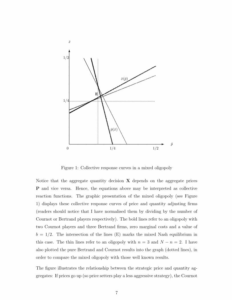
than prices of Cournot players with equal (zero) marginal costs. Figure 2 displays the

residual demand of both players: Notice that the rivals of a Cournot player consist

5The key results below hold also for less restrictive assumptions. To ease the reading of this

paper, I have decided to integrate the (rather short) proofs related to the simplified exposition into

the continuous text, while more general results are to be found in the appendix.

10

-

6

xj , xk

pj , pkppppppppppppppppppppppppppppppppppppppppppppppppppp p p p p p p p p p p p p p p p p p p p p p p p p p p p p p p p p p p p p p p p p p p p p p p p p p

pppppppppppppppppppppppppppppppppppppppppppppp p p p p p p p p p p p p p p p p p p p p p p p p p p p p p p p p p p p p p p p p p p p p p p p p p p p p p p p p p p p

x∗k x∗j

p∗jp∗k

pj(xj , p∗−j)

pk(xk, x∗−k)

Figure 2: The residual demand of a Cournot player j vis-a-vis a Bertrand firm k

of one Cournot player less, but one additional Bertrand competitor (compared to

the rivals of a price setter). For this reason, the demand function is more elastic for

the Cournot firm. If this firm plays more aggressively, it can grab demand from that

additional price setting firm—it is not possible to draw off demand from Cournot

firms, since they have fixed their output by definition. As a consequence, marginal

revenue from a price cut is higher for the Cournot players, and they will sell their

outputs at lower prices than their Bertrand rivals.

Proposition 1 Cournot players sell at lower prices than Bertrand players: pj < pk.

Proof: The quotient of (20) and (18) shows the relation between the product prices

of two firms with equal marginal costs cj = ck = 0, but different strategic situations:

pk

pj

=(1 + b(N − n− 1))(2− b + 2b(N − n))

(1 + b(N − n))(2− 3b + 2b(N − n))(21)

11

Note that this fraction has the form (AB−bB)/(AB−2Ab), with A = 1+b(N−n),

B = 2 − b + 2b(N − n) and b positive. The numerator exceeds the denominator,

since B < 2A. Hence pk > pj.2

However, a comparison of profits leads to a different result.

Proposition 2 Cournot players earn more profit than Bertrand players: πj > πk.

Proof: Using equation (21) and the fact that from (17) to (20)

πj =(1− b)(1 + b(N − n))

(1 + b(N − n− 1))· x2

j (22)

and πk =(1 + b(N − n− 2))

(1− b)(1 + b(N − n− 1))· (pk − ck)

2, (23)

yields the proportion of the profits:

πk

πj

=(1 + b(N − n− 2))(2− b + 2b(N − n))2

(1 + b(N − n))(2− 3b + 2b(N − n))2(24)

This fraction has the structure ((A − 2b)B2)/(A(B − 2b)2). As can be seen easily,

the denominator exceeds the numerator if 2Ab−B(2A−B) > 0. This condition is

always fulfilled for positive values of A, B and b, because B < 2A and 2A−B = b.2

Notice that a Bertrand firm earns less profit, but charges a higher price than a

Cournot rival. Therefore its sales are lower. Thus, the analysis of the market

position implies these results:

• In a differentiated oligopoly, comparable companies sell at different prices,

depending on their use of price or quantity strategies. To be more exact, the

quantity adjusting firm sells more, but at a lower price, than its price setting

rival.

• The strategic quantity effect outweighs the price effect. Thus, the price setting

firm is caught in an adverse situation and earns less profit than its quantity

competitor.

12

3.2 The Impact of Technology Switch-Over

Now consider a firm that decides to introduce a new technology. The results stated

above suggest that this firm suffers a strategic disadvantage in this case. Still, it

has to bear in mind that the switch-over of own technology also has an impact on

total market structure: The number of price adjusting firms increases to N −n + 1,

while the quantity of Cournot players on the market drops to n− 1. This has to be

taken into consideration when evaluating the impact of technology change on the

own market position, market performance and social benefit.

Does a firm charge a higher or a lower price when it introduces new technology?

As the technology switch-over (and therefore the switch-over of the strategy set)

lets the own residual demand uneffected, that firm would not have any incentive to

change its own quantity or prices if its competitors did not change their strategy.

However, its competitors face a new strategic situation. From their point of view,

the number of Cournot rivals on the market has decreased by one, whereas one

additional Bertrand firm competes on the market. Hence, their demand becomes

more elastic and they play more aggressively. As a result, prices of the rivals go

down and the switching firm reacts with reduced prices. From this, it follows:

Proposition 3 If a firm turns into a Bertrand player, it will charge a lower price

than it used to receive as a Cournot player: pNj,n > pN

k,n−1.

Proof: Note that we have to compare the price of a Bertrand firm to a Cournot

player on a market that consists of one Bertrand player less and an additional

Cournot player instead. Let pNj,n be the equilibrium price of a Cournot player, pN

k,n

that of a Bertrand firm in an oligopoly market with n Cournot and N −n Bertrand

players. Under the assumption that cj = ck = 0, one receives from (18) and (20)

after simple transformations:

pNj,n − pN

k,n−1 =b3(1− b)[2bN(N − n− 1) + N(2 + b)− 2nb + 3b− 2]

(1 + b(N − n− 1)) · ψ · ω (25)

where ψ = (1− b)(4 + b(6N − 4n)) + b2(2N(N − n) + (N − 1))

ω = (1− b)(4 + b(6N − 4n− 4)) + b2(2N(N − n)−N − 1)

13

For N > n ∈ N and 0 < b < 1, the numerator as well as ψ and ω are then positive.

So pNj,n − pN

k,n−1 > 0.2

How does a firm’s profit change after the technology switch-over? To see this, first

consider the remaining Cournot players.

Proposition 4 The more Bertrand firms exist, the lower are the profits of the re-

maining Cournot players: πNj,n > πN

j,n−1.

This is coherent with the overall decline in prices, which leads to lower marginal

revenue for any quantity choice.

Proof: From (17) and (22) one receives ∂πj/∂n:

∂πj

∂n=

b3(1− b)2(2 + 2b(N − n)− 3b)[4N − 8 + b((8N − 4)(N − n− 1) + 6)]

(1 + b(N − n− 1))2 · ω3

+b5(1− b)(2 + 2b(N − n)− 3b)[4N(N − n)2 − 2(N − n)(2n− 1) + N + 1]

(1 + b(N − n− 1))2 · ω3

(26)

As can be seen easily, this expression is positive for all N > 2 and n < N − 1 ∈ R+.

As the sign of the denominator is positive in the total range of 0 < n < N − 1,

the profit function has to be continous and continously differentiable there. From

the sign of the numerator follows: πNj,n > πN

j,n−1 ∀n < N, n > 2, n, N ∈ N.

Comparing profits in the two special cases, one receives that πNj,N > πN

j,N−1 and

π[2]j,2 > π

[2]j,1. 2

I am now in the position to state the strategic impact of a technology switch-over:

Proposition 5 A Cournot firm turning into a Bertrand firm suffers a strategic

disadvantage.

Proof: This statement follows directly from proposition 2 and proposition 4.

From proposition 4, we know that Cournot firms earn less when the number of

Cournot firms declines. From proposition 2, we know that Bertrand firms earn less

than Cournot firms. If a firm introduces new technology, it will turn from Cournot

14

to Bertrand competition, and the number of Cournot players on the market will be

reduced by one.2

However, the impact of a strategy change on the other price setting companies is

ambigous, because for close substitutes (b > 2/3), the output of Cournot competitors

declines in this case. Due to the adverse effect of intensified aggressiveness by the

price adjusting firms—it hits the quantity playing rivals more severely—, a reduction

of n may even result in higher profits for Bertrand players, while the Cournot rivals

earn less.

Do customers benefit from electronic commerce? At least this model framework

gives a positive answer.

Proposition 6 If one Cournot player turns into a Bertrand firm, all firms charge

lower prices.

Proof: From proposition 1, follows directly that pNj,n < pN

k,n and pNj,n−1 < pN

k,n−1.

From proposition 3, we know that pNk,n−1 < pN

j,n. Thus we can formulate the

following inequation chain: pNj,n−1 < pN

k,n−1 < pNj,n < pN

k,n. As can be seen by direct

inspection, pNj,n−1 < pN

j,n and pNk,n−1 < pN

k,n. 2

The universal price cut, initialised by the technology switch-over, eases the represen-

tative consumer’s budget constraint. Thereby, his real wealth is enlarged. While the

firms that introduce electronic commerce suffer a strategic disadvantage, costumers

benefit from the emergence of new digital production and distribution. Market

efficiency rises as well since price mark-ups on zero marginal costs shrink.

4 Conclusion

The purpose of this paper was to show that negative strategic impacts of a process

innovation on own profit occur, if in turn the company competes in prices instead of

quantities when using electronic coordination in production and distribution. There

are two main reasons for that: Firstly, the innovation involves a change in market

15

structure, the number of price setting firms increases while Cournot rivals shrink.

Even in a mixed oligopoly, this leads to fiercer competition. Secondly, turning into

a price setting firm, it suffers a strategical disadvantage compared to its rivals. Yet,

more price competition would increase market efficiency. From that point of view,

one should expect too little incentives for firms to invest in new technologies of

electronic coordination.

However, generalising this statement would overstress my arguments: In a broader

context, one has to regard effects that go in the opposite direction. It has to be taken

into consideration that new technologies are introduced precisely because costs of

production can be reduced significantly. As a consequence, producers still using

old technique may be driven out of the market. Intensity of competition might

be reduced that way. Another objection states that electronic coordination offers

vast possibilities to collect customer data. This enables companies to judge their

consumers’ preferences more precisely and may help to discriminate prices. A global

view which includes these aspects might be the topic for further research.

Appendix

The main results of this paper persist in a less restrictive framework, where all firms

produce with constant, but individual marginal costs c and earn at least zero profits.

Proposition 7 and 8 generalize proposition 1 and 2, while proposition 9 and 10

include the statement of proposition 3. Finally, proposition 11 and 12 include

the key results of this paper that are presented in proposition 5 and 6.

Proposition 7 Cournot players sell at lower prices than Bertrand players with

equal marginal costs c: pj(c) < pk(c).

Proof: See proposition 1.2

Proposition 8 Cournot players earn more profit than Bertrand players with equal

marginal costs c: πj(c) > πk(c).

Proof: See proposition 2.2

16

Proposition 9 If a firm turns into a Bertrand player, it will charge a lower price

than it used to receive as a Cournot player: pNj,n(ci) > pN

k,n−1(ci)

Proof: Note that we have to compare the price of a Bertrand firm to a Cournot

player on a market that consists of one Bertrand player less and an additional

Cournot player instead. Let pNj,n(cj) be the equilibrium price of the switching

Cournot player in an oligopoly market with n Cournot players, pNk,n(ck) that of the

new Bertrand firm in an (N, n−1)-oligopoly market. Further, denote cm the average

marginal costs of the non-switching Cournot players and cp the average marginal

costs of the non-switching Bertrand firms. Under the assumption that cj = ck = ci,

one receives from (18) and (20) after simple transformations:

pNj,n(ci)− pN

k,n−1(ci) =(b0 + a1ci + a2cm + a3cp)b

3

(1 + b(N − n− 1))(2 + b(2N − 2n− 1)) · ψ · ω (27)

where b0 = (1− b)(2 + b(2N − 2n− 1))[2Nb(N − n− 1)

+ N(2 + b)− 2nb + 3b− 2]

a1 = (1− b)b[2(N − 1) + b(4N(N − n)− 3(N − 1))]

+ b3(N − n)[2N(N − n) + N − 2n + 1]

a2 = (6b− 4)(n− 1)[1 + b(2N − 2n− 1) + b2((N − n)2 − (N − n))]

a3 = (N − n)[(1− b)[−4− b(2 + 8(N − n))− b2(4(N − 1) + 4(N − n)2)]

− b3[2(N − n)(N + n)−N − 1 + 2n]]

Note that for N > n ∈ N and 0 < b < 1, the denominator terms are then positive.

Thus, it has to be shown that the numerator is positive for all admissable values.

Notify also the necessary constraints that average Cournot and Bertrand players sell

a positive quantity, thus xNm,n−1(cm) ≥ 0 and xN

p,n−1(cp) ≥ 0. Calculus leads to:

xNp,n−1(cp) =

(1 + b(N − n− 1))(b1 + a11ci − a12cm + a13cp)

(1− b)(1 + b(N − n))(2 + b(2N − 2n− 1)) · ψ (28)

xNm,n−1(cm) =

b2 + a21ci + a22cm − a23cp

(1− b) · ψ (29)

17

where a11 = b(1− b)[2 + b(4(N − n) + 1)]

+ b3[3(N − n) + 2(N − n)2]

a12 = b(n− 1)[(1− b)[2 + b(4(N − n) + 1)]

+ b2[1 + 3(N − n) + 2(N − n)2]]

a13 = (1− b)[4 + 8Nb− 6nb + b2(4N(N − n) + n− 1)]

+ b3[2(N − n)2n + 3(N − n)n + n− 1]

a21 = b[1 + b(N − n− 1)]

a22 = (1− b)[2 + 3b(N − n)] + b2[(N − n)2 + (N − n)]

a23 = b[(1− b)(N − n) + b(N − n)2]

b1 = (1− b)[4 + 8b(N − n) + b2(4(N − n)2 − 1)]

b2 = (1− b)[2 + b(2N − 2n− 1)]

Now consider the problem

minci,cp,cm

pNj,n(ci) − pN

k,n−1(ci) (30)

s.t. xNm,n−1(cm) ≥ 0

xNp,n−1(cp) ≥ 0

Since the denomiator terms of xNm,n−1(cm) and xN

p,n−1(cp) are positive, this problem

can be transformed into the following standard linear optimization problem that can

be solved using the simplex method:

maxci,cp,cm

− b0 − a1ci − a2cm − a3cp (31)

s.t. − a11ci − a12cm + a13cp + s1 = b1

− a21ci + a22cm − a23cp + s2 = b2

ci, cm, cp ≥ 0 s1, s2 ≥ 0 (32)

18

As a result, both side conditions are binding for ci = 0 and identical marginal costs

of Cournot and Bertrand players:

cm = cp =(1− b)(2 + b(2N − 2n− 1))

2 + 2b(N − n− 1)− b2(N − n)(33)

The minimum value of the objective function is zero. Thus, pNj,n(ci) − pN

k,n−1(ci) is

strictly non-negative. 2

Proposition 10 Assume two Cournot firms with different marginal costs cj and

cm and two Bertrand firms with different marginal costs ck and cp. Further, assume

cj = ck = ci and cm = cp = cr. Then, the difference between the prices of the two

Cournot firms in an (N, n)-oligopoly market and the difference between the prices of

the two Bertrand companies in an (N, n − 1)-oligopoly market are equal: pNj,n(ci) −

pNm,n(cr) = pN

k,n−1(ci)− pNp,n−1(cr).

Proof: By calculation, one receives

pNj,n(cj)− pN

m,n(cm) =(cj − cm)(1 + b(N − n− 1))

2 + b(2N − 2n− 1)(34)

pNj,n(ck)− pN

m,n(cp) =(ck − cp)(1 + b(N − n− 1))

2 + b(2N − 2n− 1)(35)

Note the equivalence for cj = ck = ci and cm = cp = cr. 2

Proposition 11 If one Cournot player turns into a Bertrand firm, all firms charge

lower prices.

Proof: From proposition 7, follows directly that pNm,n(cr) < pN

p,n(cr) and

pNm,n−1(cr) < pN

p,n−1(cr). From proposition 10 and proposition 9, we know

that pNp,n−1(cr) < pN

m,n(cr). Thus we can formulate the following inequation chain:

pNm,n−1(cr) < pN

p,n−1(cr) < pNm,n(cr) < pN

p,n(cr). As can be seen by direct inspection,

pNm,n−1(cr) < pN

m,n(cr) and pNp,n−1(cr) < pN

p,n(cr). 2

Proposition 12 A Cournot firm turning into a Bertrand firm suffers a strategic

disadvantage.

19

Proof: Inserting (6) into (3) and rearranging the terms, gives the residual demand

xj(pj,∑n

i=1,i6=j xi,∑N

n pi):

xj(pj, .) =(1− b)− (1− b)b

∑ni=1,i 6=j xi + b

∑Nn pi

(1− b)(N − n + 1)− 1 + b(N − n + 1)

(1− b)(N − n + 1)pj (36)

Note that an own strategy switch-over lets the slope of the own residual demand

function x′j = ∂xj/∂pj unchanged. However, from proposition 9 we know that

the switching firm j lowers its price, when playing a Bertrand strategy instead of a

Cournot strategy. From the standard profit maximizing argument, we know that the

optimal mark-up on marginal costs is p∗j − cj = xj(pj, .)/x′(xj). Hence, a switch to

Bertand strategy reduces not only j’s mark-up, but also his output. Consequently

firm j’s profit declines. 2

References

Bakos, J. Y. (1997), Reducing Buyer Search Costs: Implication for Electronic Mar-

ketplaces, Management Science, Vol. 43, pp. 1676–1692.

Belleflamme, P. (2001), Oligopolistic competition, IT-use for product differentia-

tion and the productivity paradox, International Journal of Industrial Orga-

nization 19, 227–248.

Cornes, R., Hartley, R. (2001), Joint Production Games and Share Functions, Dis-

cussion Paper, Department of Economics, Keele University.

Dixit, A., Stiglitz, J. (1977), Monopolistic Competition and Optimal Product Di-

versity, American Economic Review, Vol. 67, pp. 287–308.

Guth, W. (1995), A Simple Justification of Quantity Competition and the Cournot-

Oligopoly Solution, Ifo-Studien, Vol. 41, pp. 245–257.

Klemperer, P., Meyer, M. (1989), Supply Function Equilibria in Oligopoly under

Uncertainty, Econometrica, Vol. 57, pp. 1243–1277.

Kreps, D., Scheinkman, J. (1983), Quantity Pre–commitment and Bertrand Com-

petition Yield Cournot Outcomes, Bell Journal of Economics, Vol. 14, pp.

326–337.

20

Morasch, K., Welzel, P. (2000), Emergence of Electronic Markets: Implications of

Declining Transport Costs on Firm Profits and Consumer Surplus, Beitrag Nr.

196, Volkswirtschaftliche Diskussionsreihe, Universitat Augsburg.

Selten, R. (1971), Preispolitik der Mehrproduktenunternehmung in der statischen

Theorie, Berlin et al.: Springer-Verlag.

Singh, N., Vives, X. (1984), Price and quantity competition in a differentiated duopoly,

Rand Journal of Economics, Vol. 15, pp. 546–554.

Spence, M. (1976), Product Selection, Fixed Costs and Monopolistic Competition,

Review of Economic Studies, Vol. 43, pp. 217–235.

Szidarovszky, F., Molnar, S. (1992), Bertrand, Cournot and Mixed Oligopolies, Keio

Economic Studies, Vol. 34, pp. 1–7.

Teske, P. (2002), Preis und Leistung/Internetbanking: Outsourcing als wesentlicher

Erfolgsfaktor, Frankfurter Allgemeine Zeitung, No. 83, April 10 2002, p. B4.

Vives, X. (1999), Oligopoly Pricing: Old Ideas and New Tools, Cambridge, Mas-

sachusetts et al.: MIT Press.

White, M. (1996), Mixed oligopoly, privatization and subsidization, Economics Let-

ters, Vol. 53, pp. 189–95

21