Embed Size (px)
Citation preview

Strategic Health Workforce Planning
Weihong Hu∗, Mariel S. Lavieri†, Alejandro Toriello∗, Xiang Liu†
∗H. Milton Stewart School of Industrial and Systems Engineering
Georgia Institute of Technology
Atlanta, Georgia 30332
weihongh at gatech dot edu, atoriello at isye dot gatech dot edu
†Department of Industrial and Operations Engineering
University of Michigan
Ann Arbor, Michigan 48109
{lavieri, liuxiang} at umich dot edu
April 27, 2016
Abstract
Analysts predict impending shortages in the health care workforce, yet wages for health care workers
already account for over half of U.S. health expenditures. It is thus increasingly important to adequately
plan to meet health workforce demand at reasonable cost. Using infinite linear programming method-
ology, we propose an infinite-horizon model for health workforce planning in a large health system
for a single worker class, e.g. nurses. We give a series of common-sense conditions any system of
this kind should satisfy, and use them to prove the optimality of a natural lookahead policy. We then
use real-world data to examine how such policies perform in more complex systems; in particular, our
experiments show that a natural extension of the lookahead policy performs well when incorporating
stochastic demand growth.
1

1 Introduction
Health workforce planning plays a key role in the United States and worldwide. Analysts project that by
2020 the U.S. will experience a shortage of up to 100,000 physicians, up to one million nurses and up to
250,000 public health professionals [57]. Adequate staffing of medical units has been shown to have a direct
impact in the quality of patient care [43], and also accounts for a considerable fraction of health care costs,
with wages for health care workers representing 56% of the $2.6 trillion spent on health care in the United
States in 2010 [36].
As the U.S. population continues to age [56] and demand for health care continues to grow, different
sectors of the population will compete for constrained and costly health care resources. It thus becomes
increasingly important to understand how the health care needs of the population are linked to long-term
workforce management plans of doctors, nurses and other medical personnel. The challenge is to ensure
that sufficient resources are available in the future to meet the growing health care needs of the population,
while accounting for the costs associated with meeting these needs. These workforce levels should meet
the demand for resources in the present and be positioned to meet demand for the foreseeable future [50],
an essentially infinite horizon. Furthermore, workforce plans should account for lags implied by training
new members of the workforce, attrition stemming from retirements, firings and resignations, and also the
adequate supervision of workers at different levels of the workforce hierarchy by their superiors.
Current practice has mostly focused on monitoring and evaluating health human resource systems [20],
yet a systematic framework is needed to understand the long term implications of the sequential decisions
made in those systems. Given the significant costs and the impact on health care outcomes associated with
workforce decisions, it is essential for stakeholders in large health systems to understand the role of the
planning horizon and the long-term consequences of health workforce plans.
We therefore propose to study the planning of workforce training, promotion and hiring within such
systems, with the main goal of designing a natural policy for decision makers to implement, and concurrently
determining common-sense conditions under which this policy is in fact optimal. Governments, regulatory
bodies, professional associations, representatives from the private sector and senior health system executives
may use the results presented in this paper to gain a deeper understanding on where incentives should be
placed to best meet the health workforce needs of the population. Our focus is on decisions at a health care
2

policy or public policy level (i.e. not on individual hiring and firing decisions), and thus our model includes
several stylized simplifications. The problem scale we are interested in has workforces numbering in the
thousands or the tens of thousands, e.g. state or provincial health systems, large hospital conglomerates,
or the U.S. Veterans Administration. We therefore model the workforce as a continuous flow and allow
fractional quantities in our solutions.
We also assume centralized control of the system, which may only be realistic in some cases. Neverthe-
less, even for those systems in which this is not entirely the case, the conditions we list can help decision
makers with limited control in monitoring the system’s behavior and deriving policy recommendations; this
is precisely the approach [51] take to study the U.S. pediatric nurse practitioner workforce.
Although uncertainty is present in any health system’s dynamics, the model we propose is deterministic,
and represents a first step in understanding how hiring, training and promotion interact. The deterministic
model allows for some preparation against uncertainty through sensitivity analysis. In addition, the structure
of solutions suggested by our analysis can be successfully extended to models with uncertainty; we include
computational experiments on a model with stochastic demand growth to demonstrate this.
1.1 Our Contribution
We propose a discounted, infinite linear programming model for strategic workforce planning, which in-
cludes training, promotion and hiring decision for a class of health workers within a hierarchical system. The
model takes as input a demand forecast, workforce payroll, training and hiring costs, workforce hierarchy
parameters and a discount factor. Though similar finite models have appeared in earlier work [37, 38, 39],
our focus here is to derive structural results and study workforce management policies that are provably
optimal under reasonable assumptions. Specifically, we consider the following to be our main contributions:
i) We give a series of common-sense conditions any system of this kind should satisfy under our as-
sumptions, demonstrate the pathological behavior that can occur when they are not satisfied and de-
rive useful structural properties of the optimal solutions from the conditions. Though based on our
assumptions, these conditions may help guide decision making in more complex systems.
ii) We prove that a natural lookahead policy is optimal for our model. In addition to optimizing this
model in particular, the result is useful because lookahead policies mimic how more complex models
3

may be managed in practice.
iii) We provide a two-part computational study based on real-world nursing workforce data. The first
component demonstrates the effectiveness of the lookahead policy in a more complex deterministic
system with additional detail, such as worker age. The second component shows that lookahead poli-
cies perform extremely well in a setting with stochastic demand growth, arguably the most important
source of uncertainty in our model.
The remainder of the paper is organized as follows: This section closes with a literature review. Section
2 formulates our model and states the conditions we assume. Section 3 uses the conditions to show some
structural properties of optimal solutions, proves the optimality of our proposed policy and discusses duality
and sensitivity. Section 4 discusses experiments that test our policy on more complex models, and Section 5
concludes outlining future research avenues. The Appendix contains technical proofs and some additional
modeling information.
1.2 Literature Review
Workforce planning models are not new to the industrial engineering and operations research literature,
with work stretching back several decades, such as [1, 9, 34, 41, 46, 52]. Workforce management models
have been developed to manage workforce in call centers [27], military personnel [29], medical school
budgets [16, 40], as well as to address cross-training and flexibility of the workforce [44, 58]. [11, 25,
55] provide overviews of workforce/manpower planning models, while [15] discuss the need of a greater
interface between operations and human resource management models and the complexities associated with
those models. Recent work continues to address workforce issues in operational or tactical time frames,
e.g. [10]; this focus on shorter horizons extends also to health care and emergency workforce planning
[14, 23, 26, 62]. The long-term workforce capacity planning models [6, 28, 54] are related to our work, yet
they concentrate only on the recruitment and retention of personnel without incorporating some of the other
decisions required to manage health care personnel. On the other hand, models such as [8, 61] concentrate
on skill acquisition and on-the job learning, focusing on a shorter time scale. The results in [59, 60] and the
recent survey [55] particularly highlight the need to research long-term health workforce planning, among
other areas.
4
The work in [37, 38, 39] develops a workforce planning model of the registered nursing workforce of
British Columbia. The model ranges over a 20-year planning horizon, and provides policy recommendations
on the number of nurses to train, promote and recruit to achieve specified workforce levels. Our proposed
model includes similar decisions, but is formulated over an infinite horizon. Furthermore, whereas this past
work was only numerical, we include both a theoretical analysis on the structure of optimal policies as well
as numerical experiments.
Infinite-horizon optimization has been widely applied to various operational problems, mostly via dy-
namic programming [45, 63]. However, the last two or three decades have also seen the direct study of
infinite mathematical programming models and specifically infinite linear programs for operations manage-
ment applications. Some problems studied in the literature include inventory routing [2, 3], joint replenish-
ment [4, 5], production planning [19, 48], and equipment replacement [35]. To our knowledge, although
dynamic programming has been applied to model some workforce management issues, e.g. [28, 46], infinite
linear programming has not yet been considered in the literature to address this topic. Furthermore, work-
force management possesses differences with other resource management problems that deal mostly with
products [28], which impedes the direct application of existing results.
A general reference for infinite linear programming is [7]. Our models operate in countable dimensions,
and follow the general structure of models such as [19, 31, 32, 47, 48, 49, 53]. For a recent overview of
optimization in health care, we refer the reader to [12].
2 Model Formulation and Assumptions
We consider an infinite-horizon, discounted workforce planning model with the following characteristics.
There is a deterministic demand forecast for each period, and the population of workers at the lowest level of
the system, e.g. junior nurses, must be at least equal to that period’s demand. The system has a fixed number
of levels above this first level; worker population at each higher level must be at least a fixed fraction of
the same period’s population one level below, to ensure adequate supervision. Between one period and
the next, a fixed fraction of each level’s population leaves the system, accounting for retirements, firings
and resignations. New workers may be added to any level directly via hiring, or indirectly through student
admission and training at the first level, and promotion at higher levels; there is no down-sizing, i.e. mass
5

firing to reduce workforce levels. Student populations take one period to train before entering at the first
workforce level; similarly, only workers who have been in a level for at least one period may be promoted.
We discuss how to extend our results to models with longer training in the subsequent sections.
The model is defined by the following parameters.
• n≥ 2: Number of workforce hierarchy levels.
• hk > 0: Per-period variable payroll costs for level k = 1, . . . ,n.
• ck > 0: Variable training (k = 0) or hiring (k ≥ 1) costs for level k = 0, . . . ,n.
• ck,k+1≥ 0: Variable promotion cost from level k= 1, . . . ,n−1 to k+1. Workers may only be promoted
once they have worked at a particular level for at least one period.
• γ ∈ (0,1): Discount factor, adjusted to account for cost increases. That is, if γ is the nominal discount
rate and α > 1 is the cost growth rate, then γ = αγ; this is the reciprocal of the “health care inflation.”
• dt > 0: Forecasted level-1 workforce demand for period t = 1, . . . .
• qk,k+1 ∈ (0,1): Minimum fraction of level-k workers needed at level k+1, for k = 1, . . . ,n−1.
• pk ∈ (0,1): Per-period retention rate of workers that stay in the system at level k = 0, . . . ,n from one
period to the next. The attrition rate 1− pk is the fraction of workers at level k expected to leave the
system from one period to the next; this includes firing, retirement and quitting.
• s0k : Students (k = 0) or workers in level k = 1, . . . ,n at the start of the current period, before attrition.
The model’s decision variables are:
• stk: Students (k = 0) or workers in level k = 1, . . . ,n at end of period t = 1, . . . .
• xtk: Students admitted (k = 0) or workers hired at level k = 1, . . . ,n in period t = 1, . . . .
• xtk,k+1: Workers promoted from level k = 1, . . . ,n−1 to k+1 in period t = 1, . . . .
Our strategic workforce planning problem then has the following formulation.
inf C(s,x) =∞
∑t=1
γt−1( n
∑k=0
ckxtk +
n−1
∑k=1
ck,k+1xtk,k+1 +
n
∑k=1
hkstk
)(1a)
6

s.t. st1 ≥ dt , ∀ t = 1, . . . (1b)
stk+1−qk,k+1st
k ≥ 0, ∀ k = 1, . . . ,n−1, ∀ t = 1, . . . (1c)
p1st−11 − st
1 + p0xt−10 − xt
12 + xt1 = 0, ∀ t = 1, . . . (1d)
pkst−1k − st
k + xtk−1,k− xt
k,k+1 + xtk = 0, ∀ k = 2, . . . ,n−1, ∀ t = 1, . . . (1e)
pnst−1n − st
n + xtn−1,n + xt
n = 0, ∀ t = 1, . . . (1f)
pkst−1k − xt
k,k+1 ≥ 0, ∀ k = 1, . . . ,n−1, ∀ t = 1, . . . (1g)
st ,xt ≥ 0, ∀ t = 1, . . . , (1h)
where st0 = xt
0 for t = 0, . . . . We take the feasible region to be the subset of solutions for which the objective
is well defined and finite [48]. In the model, the objective (1a) minimizes discounted cost over the infinite
horizon. The demand satisfaction constraint (1b) ensures enough level-1 workers are present to satisfy
projected demand each period, while (1c) ensures the minimum required fraction of level-(k+ 1) workers
are present to supervise level-k workers. The flow balance constraints (1d–1f) track workers present at each
level from one period to the next, and (1g) limits the promoted workers from level k to k+1 to those present
in level k for at least one period. The domain constraints (1h) ensure non-negativity of worker levels, hires,
promotions and student admissions.
Whereas most of the model’s parameters are stationary and can thus be explicitly given or recorded, the
demand forecast is an infinite sequence that cannot be explicitly given. In practical terms this forecast can
only be modeled implicitly, for instance by giving a first-period demand and a per-period growth rate. While
our results hold for an arbitrary sequence satisfying our assumptions, our policy requires explicit knowledge
of only the first few values of the sequence (two in the model as currently stated, but see Corollary 3.4 below
for an extension). For a discussion of related issues with non-stationary data in infinite-horizon optimization,
see e.g. [30].
We next list several conditions the model should satisfy. These conditions are common in many real
world settings or are reasonable approximations, and are necessary for most of our subsequent results.
Many are also necessary to avoid pathological behavior. We begin with technical assumptions.
Assumption 2.1 (Technical assumptions).
7

i) Finite total demand: Total discounted demand converges.
∞
∑t=1
γt−1dt < ∞ (2a)
ii) Linear costs: The objective function is linear with respect to the decision variables s and x.
The former assumption is necessary to have a finite objective and thus a feasible problem. The latter
is required to apply linear programming techniques. Though large changes in a system’s workforce could
render some costs non-linear (e.g. a large increase in hiring leading to an increase in hiring and payroll
costs because of the labor market’s supply), our results suggest that in the long run moderate decisions
predominate, and thus the assumption of linearity is reasonable.
Assumption 2.2 (Growing demand). The sequence (dt) is non-decreasing.
dt ≤ dt+1, ∀ t = 1, . . . (2b)
This assumption reflects most contemporary health care systems in which demand is expected to grow
for the foreseeable future, and ensures that training and promotion will be perpetually necessary within the
system. As discussed by [21], given changes in the demographics of the population, as well as expanded
coverage under the Affordable Care Act, demand for primary care services in the United States is expected to
grow by 14% by 2025. This expected growth in demand for health care workers is not unique to the United
States; it is estimated that an additional 1.9 billion people will seek access to health care by 2035 [17]. In
more general cases, even if demand is only expected to be eventually non-decreasing, our conclusions can
be applied starting at the period where non-decreasing growth begins, with a finite model accounting for the
system in preceding periods.
The first non-technical assumption concerns the relative costs of payroll, promotion and hiring.
Assumption 2.3 (Promotion is preferable). Even when factoring attrition, payroll costs and discounting,
promotion is cheaper than hiring.
c0
γ p0≤ c1,
ck +hk
γ pk+ ck,k+1 ≤ ck+1, ∀ k = 1, . . . ,n−1 (2c)
8

If this assumption does not hold at some level in the hierarchy, there is no incentive to train and promote
from within beyond that point. This condition should be satisfied by many workforce systems, both in health
care and in other industries.
The next assumption is slightly more specific to the health care industry, but still common in other
industries.
Assumption 2.4 (Non-increasing retention). The hierarchy does not tend to become top-heavy:
pk ≥ pk+1, ∀ k = 1, . . . ,n−1 (2d)
This assumption is natural in health care hierarchies such as nursing, where higher-level workers are
usually older, since older workers tend to retire or leave the system for other reasons at a higher rate. The
assumption is more problematic, for example, in industries where tenure guarantees at an intermediate level
imply an unnaturally high attrition at lower levels.
For some of our results, it is necessary to further strengthen the previous assumption.
Assumption 2.4’ (Equal retention). Retention and attrition are equal at all hierarchy levels:
pk = pk+1, ∀ k = 1, . . . ,n−1 (2d’)
Though it appears restrictive, in many real-world systems the top and bottom retention rates in fact only
differ by a few percentage points [37, 38, 39].
Assumption 2.5 (Non-decreasing payroll). Salaries increase within the hierarchy, even when accounting
for attrition:
hk
1− γ pk≤ hk+1
1− γ pk+1, ∀ k = 1, . . . ,n−1 (2e)
As the next example shows, this condition prevents undesirable behavior.
Example 1 (Down-sizing by promotion). Consider a two-level system which is drastically over-staffed. Let
dt = ε for all t, where ε > 0 is a small positive number, and let s01≫ ε . If (2e) is not satisfied, it may be
9

optimal because of (2d) to promote all but ε workers to level 2, effectively down-sizing the workforce by
promoting most of it, and achieving lower costs in the process. Such behavior could lead to detrimental side
effects, such as poor morale in the remaining workforce.
Assumption 2.6 (Moderate demand growth). Demand does not grow too quickly:
dt+1
dt≤ pmin
qmax, ∀ t = 1, . . . , (2f)
where pmin = mink pk and qmax = maxk qk,k+1.
Intuitively, the assumption ensures enough worker population at each level to promote to the next level
as demand grows; it is easily satisfied in most systems. For example, if n = 2, p1 = p2 = 0.8 and q12 = 0.25,
(2f) requires the demand growth to be no more than 320% per period, a condition met in virtually any
system. Furthermore, as the next example shows, when this assumption is not met, the planning horizon
necessary to compute an optimal solution may be arbitrarily long.
Example 2 (Excessive demand growth). We consider a two-level system that experiences excessive demand
growth for a given number of periods, and constant demand thereafter. To simplify the numbers in the
example, we set p1 = p2 = q12 = 1. For a fixed m≥ 2 let
dm1 = 1, dm
t =
2t−1−1, t = 2, . . . ,m
2m−1−1, t = m+1, . . .,
and s00 = 0, s0
1 = s02 = 1; note that dt+1/dt > p1/q12 = 1 for t = 2, . . . ,m−1. Table 1 details the first demand
values in the sequence, for m = 3,4,5. The table also lists a solution that satisfies demand without any
hiring, which can be made optimal by choosing large enough hiring costs. Although projected demand for
the first three periods is identical in all cases, the optimal number of students admitted in the first period
changes with m; for general m, we get x10 = (2m−2−1)/2m−3. In other words, the current period’s decision
may depend on a horizon of arbitrary length m.
As Example 2 suggests, the condition (2f) can be relaxed; we include the best possible condition of this
kind we could derive in the Appendix (see the proof of Claim A.3). However, (2f) is much simpler to state
10

t 1 2 3 4 5 · · ·d3
t 1 1 3 3 3 · · ·xt
0 1 3 0 0 0 · · ·st
1 1 3/2 3 3 3 · · ·st
2 1 3/2 3 3 3 · · ·d4
t 1 1 3 7 7 · · ·xt
0 3/2 7/2 7 0 0 · · ·st
1 1 3/2 7/2 7 7 · · ·st
2 1 3/2 7/2 7 7 · · ·d5
t 1 1 3 7 15 · · ·xt
0 7/4 15/4 15/2 15 0 · · ·st
1 1 15/8 15/4 15/2 15 · · ·st
2 1 15/8 15/4 15/2 15 · · ·
Table 1: Sample demand sequences and solutions with no hiring for m = 3,4,5 in Example 2.
and suffices for any practical situation.
3 Optimal System Behavior
We begin our characterization of optimal solutions of (1) by outlining structural properties satisfied in mod-
els that meet our assumptions. We include only simple proofs here and relegate any complex proof to the
Appendix.
Lemma 3.1 (No unnecessary hiring). Suppose the model parameters satisfy Assumptions 2.1 through 2.3.
There is an optimal solution of (1) in which no hiring takes place when promotion is possible:
xt1 = 0, ∀ t = 2, . . . (3a)
(pkst−1k − xt
k,k+1)xtk+1 = 0, ∀ k = 1, . . . ,n−1, ∀ t = 1, . . . (3b)
Proof. If a solution does not satisfy either condition, a simple substitution produces another solution with
equal or lesser objective that does satisfy the conditions. �
Lemma 3.2 (No excess training or promotion). Suppose Assumptions 2.1, 2.2, 2.3, 2.5 and 2.6 hold. Fur-
thermore, suppose either Assumption 2.4 holds and n = 2, or Assumption 2.4’ holds. Then there is an
11

optimal solution of (1) in which no excess promotion or student admittance occurs:
(st1−dt)xt−1
0 = 0, ∀ t = 2, . . . (4a)
(stk+1−qk,k+1st
k)xtk,k+1 = 0, ∀ k = 1, . . . ,n−1, ∀ t = 1, . . . (4b)
Like the preceding lemma, Lemma 3.2 follows from applying a substitution or perturbation to any
solution that does not satisfy it. However, unlike in the hiring case, a perturbation in promotion has ripple
effects in higher levels of the hierarchy and in later periods that render it much more complex.
With these two structural properties in place, we are able to characterize optimal solutions of (1). Con-
sider the two-period restriction of (1) given by
minn
∑k=0
ck(x1k + γx2
k)+n−1
∑k=1
ck,k+1(x1k,k+1 + γx2
k,k+1)+n
∑k=1
hk(s1k + γs2
k) (5a)
s.t. st1 ≥ dt , ∀ t = 1,2 (5b)
stk+1−qk,k+1st
k ≥ 0, ∀ k = 1, . . . ,n−1, ∀ t = 1,2 (5c)
p1st−11 − st
1 + p0xt−10 − xt
12 + xt1 = 0, ∀ t = 1,2 (5d)
pkst−1k − st
k + xtk−1,k− xt
k,k+1 + xtk = 0, ∀ k = 2, . . . ,n−1, ∀ t = 1,2 (5e)
pnst−1n − st
n + xtn−1,n + xt
n = 0, ∀ t = 1,2 (5f)
pkst−1k − xt
k,k+1 ≥ 0, ∀ k = 1, . . . ,n−1, ∀ t = 1,2 (5g)
st ,xt ≥ 0, ∀ t = 1,2, (5h)
A one-period lookahead policy constructs a solution to (1) by iteratively solving (5), fixing the variables for
t = 1, stepping one period forward by relabeling t← t+1 for all variables and parameters, and repeating the
process. In practice, this corresponds to a decision maker planning the current period’s promotion, training
and hiring based on current demand and the next period’s forecasted demand, while ignoring demand for
subsequent periods.
Theorem 3.3 (Optimality of one-period lookahead policy). Suppose Assumptions 2.1, 2.2, 2.3, 2.5 and 2.6
are satisfied. Suppose either Assumption 2.4 holds and n = 2, or Assumption 2.4’ holds. Then one-period
12

lookahead policies are optimal.
Corollary 3.4 (Increased training time). Suppose students require L≥ 1 periods to train instead of one, with
all other system characteristics remaining the same. Under the conditions of Theorem 3.3, L-period looka-
head policies are optimal, where an L-period lookahead is defined analogously to a one-period lookahead
but with L additional periods instead of one.
Proof. The proof of Theorem 3.3 still applies; we are simply relabeling level-0 variables. �
These results indicate that good workforce planning decisions can be made using a minimal amount of
forecasted information, which strengthens the robustness of the resulting solution since forecasts of more
distant demand naturally tend to be less reliable. This also places our result within the context of solution
and forecast horizons; see, e.g., [18] for formal definitions and discussion.
Moreover, lookahead policies mimic how such large workforce systems can be managed in practice.
The optimization of the lookahead model (5) is split into two separate sets of decisions: First, the model
decides how to meet the current period’s demand (period 1) at minimum cost given the current workforce
levels and the new entering workforce; this is a more tactical, short-term decision in which the only recourse
is hiring and promotion. Then, based on this decision, the model strategically projects ahead one period to
decide the number of students to admit into training, so that the next period’s demand can be met also at
minimum cost. In (5), the second-period variables are only used to determine this admission quantity, and
are not in fact implemented.
Although the lookahead policy given by (5) optimally solves the original infinite-horizon problem, it is
worth noting that this policy is quite simple to implement. At every period, it involves only the solution of
a small, two-period LP; for example, in a system with four hierarchy levels, the number of variables in the
model is 24, a model size that can be solved even in spreadsheet optimization packages in a few seconds
or less. This suggests that these policies could be useful in more complex settings; we explore this idea
experimentally in Section 4.
Another important question related to (1) is duality. A dual satisfying the typical complementary rela-
tionships can shed additional light on the structure of optimal solutions to (1). Furthermore, optimal dual
prices may also be useful as indicators of the model’s sensitivity to parameters such as demand. However,
13

the infinite horizon implies significant technical complications and gives rise to pathologies not encountered
in the finite case.
Extending the typical LP dual construction to (1) yields
sup D(µ,λ ,η) =∞
∑t=1
dt µt1− p0s0
0λ11 −
n−1
∑k=1
pks0k(λ
1k +η
1k,k+1)− pns0
nλ1n (6a)
s.t. µtk−qk,k+1µ
tk+1−λ
tk + pkλ
t+1k + pkη
t+1k,k+1 ≤ γ
t−1hk, ∀ k = 1, . . . ,n−1, ∀ t = 1, . . . (6b)
µtn−λ
tn + pnλ
t+1n ≤ γ
t−1hn, ∀ t = 1, . . . (6c)
p0λt1 ≤ γ
t−2c0, ∀ t = 2, . . . (6d)
λtk ≤ γ
t−1ck, ∀ k = 1, . . . ,n, ∀ t = 1, . . . (6e)
−λtk +λ
tk+1−η
tk,k+1 ≤ γ
t−1ck,k+1, ∀ k = 1, . . . ,n−1, ∀ t = 1, . . . (6f)
µt ,η t ≥ 0, λ
t unrestricted, ∀ t = 1, . . . , (6g)
where we similarly define the feasible region as a subset of the points for which the objective is well defined
and finite. However, this model does not satisfy strong or even weak duality with (1).
Example 3 (No weak duality; adapted from [53]). Suppose s0n > 0 and let M > 0. Define λ t
n = −M/ptn,
∀ t = 1, . . . , and set all other variables to zero. The solution is feasible for (6), and its objective function
value is positive and goes to infinity as M→∞. However, (1) is clearly feasible and bounded below by zero.
The following result addresses this problem.
Theorem 3.5. Suppose we can change the equality constraints (1d–1f) to greater-than-or-equal constraints
(and thus impose λ t ≥ 0) for all but a finite number of indices t without affecting optimality in (1). Let (s, x)
and (µ, λ , η) be feasible for (1) and (6) respectively.
i) Weak duality: D(µ, λ , η)≤C(s, x).
ii) Strong duality: Both solutions are optimal and D(µ, λ , η) = C(s, x) if and only if complementary
slackness holds (in the usual sense) and transversality [48, 49, 53] holds:
liminft→∞
p0λt+11 xt
0 +n−1
∑k=1
pk(λt+1k + η
t+1k )st
k + pnλt+1n st
n = 0. (7)
14

Proof. If all constraints eventually become greater-than-or-equal, then the off-diagonal constraint matrix of
(1) in inequality form is eventually non-negative, implying that [48, Assumption 3.1] holds, and thus the
results follow from [48, Theorems 3.3 and 3.7]. �
Corollary 3.6. The conditions of Theorem 3.5 apply, and therefore weak and strong duality hold, if demand
is eventually non-decreasing.
The results in [48] imply we can use optimal solutions of (6) as shadow prices to perform sensitivity
analysis on (1).
Example 4 (Sensitivity analysis). Consider a two-level system in which the incoming worker populations
in period 1 require some promotion from level 1 to level 2, with enough level-1 workers remaining after
promotion to meet demand in period 1 but not later. Based on these initial conditions and Assumptions 2.1
through 2.6, Lemmas 3.1 and 3.2 imply the following structure to the optimal solution:
xt1 = xt
2 = 0, xt0,x
t12 > 0, xt
12 < p1st−11 , st
2 = q12st1, ∀ t = 1, . . .
s11 > d1; st
1 = dt , ∀ t = 2, . . .
The solution for (6) that satisfies complementary slackness and transversality is:
µ11 = 0
µt1 =
γ t−2c0
p0
(1− γ p1 +q12(1− γ p2)
)+ γ
t−1q12c12(1− γ p2)
+ γt−1(h1 +q12h2), ∀ t = 2, . . .
µ12 =
11+q12
(c0
p0(p1− p2)+ c12(1− γ p2)+(h2−h1)
)µ
t2 = γ
t−2(1− γ p2)
(c0
p0+ γc12
)+ γ
t−1h2, ∀ t = 2, . . .
λ11 =
11+q12
(c0
p0(p1 +q12 p2)−q12c12(1− γ p2)− (h1 +q12h2)
)λ
t1 =
γ t−2c0
p0, ∀ t = 2, . . .
λ12 =
11+q12
(c0
p0(p1 +q12 p2)+ c12(1+ γq12 p2)− (h1 +q12h2)
)
15

λt2 = γ
t−2(
c0
p0+ γc12
), ∀ t = 2, . . .
ηt12 = 0, ∀ t = 1, . . .
It can be verified that this solution is dual feasible provided the assumptions hold. Suppose in particular
that demand grows based on a rate 1 < β < 1/γ , so that dt = β t−1d1. It follows that
∞
∑t=1
dt µt1 = d1
[c0
γ p0
(1− γ p1 +q12(1− γ p2)
)+q12c12(1− γ p2)+h1 +q12h2
]βγ
1−βγ.
This expression indicates how the optimal cost would change if either d1 or β vary slightly from their given
values.
4 Computational Study
To evaluate the efficacy of our proposed models and policies, we performed computational experiments
based on the British Columbia nursing workforce described in [37, 38, 39]. Health care human resource
data is more readily available from Canadian provinces because of their centralized control of health care.
However, similar data from U.S. systems can be used within a model such as ours to derive policy recom-
mendations, e.g. [51], even though U.S. health systems are usually de-centralized.
We first discuss the performance of lookahead policies applied to more complex, albeit deterministic,
settings. We then develop a simulation model that considers uncertainty in demand growth and evaluate the
performance of our lookahead policies in this setting.
4.1 Deterministic experiments
While model 1 provides useful insights into the behavior of strategic workforce planning models, possible
extensions include the differentiation of workers by age (as it affects attrition rates), and the extension of the
length of student training (to four years). In order to evaluate the performance of our lookahead policies,
we began by solving the problem over a 25-year planning horizon (a full information model) and used the
solution to the first 20 years as our benchmark. We then compared the results to a solution obtained by
implementing a four-year lookahead policy of this extended model.
16

Figure 1 outlines the structure of the extended model and its parameters (see further model description
in the Appendix). Students are admitted into the training program, where they take four years to train before
entering the workforce. The probabilities of students continuing their education depend on the school year
of the student (with greater attrition in the first year of the program). After graduation, students enter the first
workforce level as direct care nurses. In level 1, the number of workers has to meet current demand. This
demand is met by workers that have not retired or been promoted, graduates from the training program and
workers hired externally. Level 2 consists of nurse managers, a supervisory position to the first level; nurse
managers are either hired externally or promoted from the first workforce level. To account for transition
shock and adaptation to the profession [24], we assume that Level-1 workers must have worked for at least
one year before being promoted into the second workforce level. In both levels, retention rates depend on
the age of the workers. The average retention in level 2 is slightly higher than the average retention in level
1, which would violate Assumption 2.4 if the averages applied to all age groups. Furthermore, since the
parameter is age-dependent in this model, the actual retention in each level depends on the age distribution
of the worker population. This difference in attrition rates did not impact our results, further supporting the
robustness of our findings. We set the discount factor to γ = 0.95.
We tested the model in nine scenarios. Among the nine scenarios, the baseline scenario represents the
estimated demand in British Columbia, Canada, starting in 2007; we calculated demand by extrapolating
the population growth between 1996 and 2006 [13]. Scenarios 1 through 4 evaluate the impact of different
demand growth rates. Scenario 5 evaluates the impact of limiting the growth of the training program.
Scenarios 6, 7 and 8 evaluate the performance of the lookahead policy in extreme conditions where demand
has a peak, hiring growth is limited, and costs are varied. The parameter characteristics and descriptions of
the scenarios are summarized in the following list.
Baseline Scenario Fixed demand growth rate of 1.25% per year. Projected demand growth in British
Columbia, Canada.
Scenario 1 Fixed demand growth rate of 0.01% per year. Very low demand growth.
Scenario 2 Fixed demand growth rate of 2.5% per year. High demand growth.
Scenario 3 Linearly accelerating demand growth from 0% per year to 2.5% per year over 25 years.
17

Students4 years in school
Admissions$57,991/student
Workforce Level 1Meet growing demand Payroll cost $87,600/worker/yr
Entering Probability91%
Hiring Level 1$113,880/worker
Workforce Level 2Supervise Level 1 workers (1 level 2 : 10.5 level 1)Payroll cost $95,104/worker/yrHas worked in Level 1 for at least 1 yr
Hiring Level 2$283,800/worker
Attrition Rateby School Year
10%, 2%, and 5% in year 1, 2, and 3
Age-dependent Attrition
Prom
otio
ns$2
8,50
0/w
orke
rAge-dependent Attrition
DecisionsUnit Cost
Figure 1: Flow chart of model used in computational examples.
Scenario 4 Linearly decelerating demand growth from 2.5% per year to 0% per year over 25 years.
Scenario 5 Fixed demand growth rate of 1.25% per year and student population growth limited to no more
than 1% per year. Major restrictions in training growth.
Scenario 6 Fixed demand growth rate of 1.25% per year in years 1 through 9 and 11 through 25, demand
doubled in year 10. Level-1 hiring growth limited to no more than 50% per year. This scenario
simulated a sudden jump of demand, which might be due to a drastic change in roles and scope of
practice of the workforce. We assumed that drastic changes in the number of workers hired could not
be made without incurring very large recruitment costs.
Scenario 7 Fixed demand growth rate of 1.25% per year in years 1 through 9 and 11 through 25, demand
doubled in year 10. Level-1 hiring growth limited to no more than 50% per year, and zero student
admission cost. In addition to the jump in demand and limited hiring growth, we eliminated the
admission cost to increase the incentive to admit students in advance and thus potentially undermine
18

the four-year lookahead model.
Scenario 8 Fixed demand growth rate of 1.25% per year in years 1 through 9 and 11 through 25, demand
doubled in year 10. Level-1 hiring growth limited to no more than 50% per year, and zero level-1
payroll cost. In addition to the jump in demand and limited hiring growth, we eliminated the level-1
payroll cost to increase the incentive to admit students in advance and thus potentially undermine the
four-year lookahead model.
We compared the solutions obtained using the full information model and the lookahead model. Figure
2 shows results for the baseline scenario and scenarios 1 through 5. In these scenarios, we obtained the same
solutions using the full information and the lookahead models. The lookahead model was robust in these
scenarios, even if Assumption 2.4 was slightly violated by our system’s parameters. Even in Scenario 5,
where education growth was drastically limited, the full information model did not differ from the lookahead
policy because training students a year in advance incurred extra payroll costs, making early training more
expensive than hiring. Though education growth was limited, hires served as a back-up action in Scenario 5
and made the lookahead and the full information methods operate identically.
Figure 3 shows results for scenarios 6, 7, and 8; in this case, the lookahead policy resulted in slightly
higher total costs. Compared to the full information solution, the percentage differences in total cost were
only 0.026%, 0.129%, and 0.014% respectively. The lookahead model resulted in more admissions, more
level-2 hirings, and fewer level-1 hirings than the full information model. Since level-1 hiring was limited,
fewer level-1 workers were hired and more students were trained as an alternative. Level-2 workers were
hired when the model reached a point where promotions could not meet the level-2 workforce demand due
to the insufficient number of level-1 workers. The lookahead model failed to anticipate future changes in
demand, not training sufficient students nor hiring sufficient level-1 workers in advance.
Overall, the lookahead policy showed robustness in the nine scenarios modeled. In the most extreme
scenarios, where demand had a sudden jump and hirings or admissions were limited, the lookahead policy
and the full information policy still showed very little difference, particularly in total cost.
19

0
10000
20000
30000
40000
50000
60000
70000
80000
90000
100000
Num
ber o
f Adm
ission
s/Hirings
Scenarios/Policies
Admissions and Hirings BreakdownBaseline scenario and scenarios 1 through 5
# Lv.2 WorkerHirings
# Lv.1 WorkerHirings
# StudentAdmissions
Figure 2: Breakdown of the total number of admissions and hirings in baseline scenario and scenarios 1through 5 over the course of 20 years.
228000
229000
230000
231000
232000
233000
234000
235000
236000
237000
Scenario 6Full Info
Scenario 6Lookahead
Scenario 7Full Info
Scenario 7Lookahead
Scenario 8Full Info
Scenario 8Lookahead
Num
ber o
f Adm
ission
s/Hirings
Scenarios/Policies
Admissions and Hirings Breakdownscenarios 6 through 8
# Lv.2 WorkerHirings
# Lv.1 WorkerHirings
# StudentAdmissions
Figure 3: Breakdown of the total number of admissions and hirings in scenarios 6 through 8 over the courseof 20 years.
20

4.2 Experiments with stochastic demand growth
To further evaluate the lookahead policy, we examined the performance of our model in a stochastic setting
where the demand growth rate in each year (denoted ρ) is an i.i.d. random variable uniformly distributed
between 0% and 2.5% (the mean growth rate is thus kept at 1.25%, as in the deterministic baseline scenario
[39]).
We applied the lookahead policy sequentially. After the simulated demand dt is realized in year t, we
project year (t+1)’s demand to be dt+1 =(1+(1+δ )E[ρ]
)dt , where δ is a forecast factor used to represent
the planner’s level of risk-aversion. When δ > 0, the planner assumes demand grows faster than the mean;
for δ < 0, the planner assumes the demand grows slower than the mean; for δ = 0, the planner plans for
the expected growth. After solving the lookahead model for years t and t +1, the process steps forward one
year, true demand in t +1 is observed, and hiring decisions are made if the workforce is insufficient to meet
the demand. The algorithm proceeds to the next period and the look-ahead policy is sequentially applied.
This procedure iterates until period 20. In our simulation, each policy was solved with 2000 replications.
We considered two benchmarks for the lookahead policies. The first is the full information model; as
in the deterministic experiments, the full information solution solves a single LP with full (deterministic)
access to the uncertain parameters. In the stochastic case, this implies solving one full information LP for
every simulated replication and averaging the resulting costs. Because this solution has earlier access to the
uncertain data, it provides a lower bound on any policy’s cost.
In addition, we included as a second benchmark a naıve policy implemented without resorting to our
LP. This policy sets workforce level targets for the current period based on demand or incoming level-1
workforce, whichever is greater, and meets these levels by promoting as much as possible before hiring.
The policy then determines student admissions using the following simple rule: If the level-1 workforce
exactly meets demand, admissions are scaled up from the previous year based on expected demand growth.
Conversely, if the level-1 workforce exceeds demand, admissions are scaled down by the same percentage
that the workforce exceeds demand by. For example, if workforce is 105% of demand, admissions are set to
95% of the previous year’s number.
As shown in Figure 4, by varying the forecast factor δ over 1% increments between −100% and 100%,
the lookahead policy achieves lowest cost at δ ∗ = −33% (the best delta policy). All lookahead policies
21
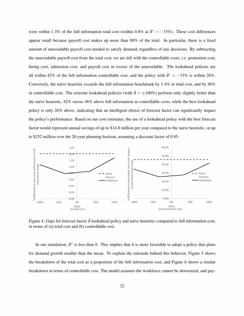
were within 1.3% of the full information total cost (within 0.8% at δ ∗ = −33%). These cost differences
appear small because payroll cost makes up more than 90% of the total. In particular, there is a fixed
amount of unavoidable payroll cost needed to satisfy demand, regardless of any decisions. By subtracting
the unavoidable payroll cost from the total cost, we are left with the controllable costs, i.e. promotion cost,
hiring cost, admission cost, and payroll cost in excess of the unavoidable. The lookahead policies are
all within 42% of the full information controllable cost, and the policy with δ ∗ = −33% is within 26%.
Conversely, the naıve heuristic exceeds the full information benchmark by 1.4% in total cost, and by 46%
in controllable cost. The extreme lookahead policies (with δ = ±100%) perform only slightly better than
the naıve heuristic, 42% versus 46% above full information in controllable costs, while the best lookahead
policy is only 26% above, indicating that an intelligent choice of forecast factor can significantly impact
the policy’s performance: Based on our cost estimates, the use of a lookahead policy with the best forecast
factor would represent annual savings of up to $14.8 million per year compared to the naıve heuristic, or up
to $252 million over the 20-year planning horizon, assuming a discount factor of 0.95.
0.0%
0.2%
0.4%
0.6%
0.8%
1.0%
1.2%
1.4%
1.6%
-100% -50% 0% 50% 100%
%difference
intotalcostswith
respecttofulll
inform
ationmodel
Delta(a) Total Cost
NaiveheuristicLookahead
0.0%
10.0%
20.0%
30.0%
40.0%
50.0%
60.0%
-100% -50% 0% 50% 100%
%difference
incontrollablecostsw
ithrespect
tofulllinform
ationmodel
Delta(b) Controllable Cost
NaiveheuristicLookahead
Figure 4: Gaps for forecast factor δ lookahead policy and naıve heuristic compared to full information cost,in terms of (a) total cost and (b) controllable cost.
In our simulation, δ ∗ is less than 0. This implies that it is more favorable to adopt a policy that plans
for demand growth smaller than the mean. To explain the rationale behind this behavior, Figure 5 shows
the breakdown of the total cost as a proportion of the full information cost, and Figure 6 shows a similar
breakdown in terms of controllable cost. The model assumes the workforce cannot be downsized, and pay-
22

92% 94% 96% 98% 100% 102% 104% 106%
Fullinformation
Bestdelta (δ=-33%)
Planforthemean(δ=0)
Planfornogrowth(δ=-100%)
Planforhighestgrowth(δ=100%)
Naïveheuristic
Notraining
PayrollcostAdmissionCostHiringCostPromotionCost
Figure 5: Breakdown of total cost under different policies: payroll costs dominate the other costs.
0% 50% 100% 150% 200% 250% 300%
Fullinformation
Bestdelta (δ=-33%)
Planforthemean(δ=0)
Planfornogrowth(δ=-100%)
Planforhighestgrowth(δ=100%)
Naïveheuristic
Notraining
PayrollCostinExcessAdmissionCostHiringCostPromotionCost
Figure 6: Breakdown of controllable cost under different policies: look-ahead policies stay within 40% fromfull information model with minimal gap of 22% at δ ∗ = 33%.
roll cost makes up more than 90% of the total. Therefore, an oversized workforce will remain in the system
many years and will thus increase the cost dramatically. To further explore this idea, we also simulated a
policy with no training that directly hires 100% of its workforce. However, the no-training policy performed
far worse, with a gap of 4.7% in terms of total cost or 150% in controllable cost. Furthermore, the full in-
formation solution does not have any excess hiring costs, as these can be completely avoided with complete
access to information; therefore, it is likely that the true optimal cost is closer to our best lookahead policy
than to this lower bound.
23

5 Conclusions
This paper contributes a new modeling framework for strategic health workforce planning. Through infinite-
horizon optimization, we are able to model the long-term implications of training, hiring and promotion
decisions made within a health care system. Our results (cf. Theorem 3.3 and Corollary 3.4) indicate that
very short planning horizons suffice to determine optimal decisions when employing the model in a rolling
horizon framework. We obtained these results under a set of mild assumptions (Assumptions 2.1 through
2.6) that correspond to reasonable real-world conditions, such as the requirement that payroll increase in the
workforce hierarchy. Using real-world data from British Columbia, we further demonstrate how lookahead
policies perform well in a variety of situations that generalize our base model, specifically in the case of
uncertain demand growth. These results are particularly useful, as the lookahead solution mirrors workforce
management policies that could be implemented in practice. Models such as the one we propose can be used
to obtain qualitative checks on whether a particular health workforce system is behaving optimally, or what
conditions it must meet to do so. For example, in [51] the authors apply a similar model to derive policy
recommendations for the U.S. pediatric nurse practitioner workforce.
A next step in our work is to directly model and optimize the system’s uncertainty, specifically in demand
growth or retention rates [42]. It is important to understand whether the conditions we develop in this work
and their structural consequences (or appropriate modifications) still hold in more general settings. The more
nuanced analysis required in this case may give insight into the impact of uncertainty on health workforce
costs and management decisions; for example, [22, 33] investigate similar questions for short-term nurse
staffing. From a theoretical perspective, the infinite linear programming tools we use still apply in the
presence of uncertain demand growth or retention, provided these can be modeled as finite-support random
variables.
Because this work is applied to guide strategic health workforce decisions, we can formulate more
realistic models by incorporating other elements. For instance, (1) could be expanded to include a variety of
health care providers and changes in scopes of practice. Assuming that the interaction of all worker types
with demand is linear, multiple worker types can be incorporated in models similar to (1), by differentiating
across both type and level, where each worker type includes its own hierarchy with its own supervision
constraints (1c) and dynamics, but the multiple types serve patient demand jointly.
24

By providing an initial understanding of this infinite-horizon model, our goal is to move a step forward
in the field of strategic health workforce planning, and to motivate others to continue doing research in this
important application.
Acknowledgments
The authors thank the associate editor and two anonymous referees for their valuable comments and sug-
gestions.
References
[1] W.J. Abernathy, N. Baloff, J.C. Hershey, and S. Wandel. A Three-Stage Manpower Planning and
Scheduling Model–A Service-Sector Example. Operations Research, 21:693–711, 1973.
[2] D. Adelman. Price-Directed Replenishment of Subsets: Methodology and its Application to Inventory
Routing. Manufacturing and Service Operations Management, 5:348–371, 2003.
[3] D. Adelman. A Price-Directed Approach to Stochastic Inventory/Routing. Operations Research,
52:499–514, 2004.
[4] D. Adelman and D. Klabjan. Duality and Existence of Optimal Policies in Generalized Joint Replen-
ishment. Mathematics of Operations Research, 30:28–50, 2005.
[5] D. Adelman and D. Klabjan. Computing Near-Optimal Policies in Generalized Joint Replenishment.
INFORMS Journal on Computing, 24:148–164, 2011.
[6] H.S. Ahn, R. Righter, and J.G. Shanthikumar. Staffing decisions for heterogeneous workers with
turnover. Mathematical Methods of Operations Research, 62:499–514, 2005.
[7] E.J. Anderson and P. Nash. Linear Programming in Infinite-Dimensional Spaces. John Wiley & Sons,
Inc., Chichester, 1987.
[8] A. Arlotto, S.E. Chick, and N. Gans. Optimal Hiring and Retention Policies for Heterogeneous Work-
ers who Learn. Management Science, 2013. Forthcoming.
25

[9] W. Balinsky and A. Reisman. Some Manpower Planning Models Based on Levels of Educational
Attainment. Management Science, 18:691–705, 1972.
[10] J.F. Bard and L. Wan. Workforce design with movement restrictions between workstation groups.
Manufacturing and Service Operations Management, 10:24–42, 2008.
[11] D.J. Bartholomew, A.F. Forbes, and S.I. McClean. Statistical Techniques for Manpower Planning.
John Wiley & Sons, Inc., second edition, 1991.
[12] S. Batun and M.A. Begen. Optimization in healthcare delivery modeling: Methods and applications.
In Handbook of Healthcare Operations Management, pages 75–119. Springer, 2013.
[13] BC Statistics. Population Estimates, British Columbia. Available on-line at http://www.bcstats.
gov.bc.ca, April 2013.
[14] D. Bienstock and A.C. Zenteno. Models for managing the impact of an epidemic. Working pa-
per, Department of Industrial Engineering and Operations Research, Columbia University. Version
Sat.Mar.10.153610.2012. Available at http://www.columbia.edu/~dano/papers/bz.pdf, 2012.
[15] J. Boudreau, W. Hopp, J.O. McClain, and L.J. Thomas. On the interface between operations and human
resources management. Manufacturing and Service Operations Management, 5:179–202, 2003.
[16] M.L. Brandeau, D.S.P. Hopkins, and K.L. Melmon. An integrated budget model for medical school
financial planning. Operations Research, 35:684–703, 1987.
[17] J. Campbell, G. Dussault, J. Buchan, F. Pozo-Martin, M. Guerra Arias, C. Leone, A. Siyam, and
G. Cometto. A Universal Truth: No Health Without a Workforce. Technical report, Global Health
Workforce Alliance and World Health Organization, Geneva, 2013. Forum Report, Third Global Fo-
rum on Human Resources for Health, Recife, Brazil.
[18] T. Cheevaprawatdomrong, I.E. Schochetman, R.L. Smith, and A. Garcia. Solution and Forecast Hori-
zons for Infinite-Horizon Nonhomogeneous Markov Decision Processes. Mathematics of Operations
Research, 32:51–72, 2007.
26

[19] W.P. Cross, H.E. Romeijn, and R.L. Smith. Approximating Extreme Points of Infinite Dimensional
Convex Sets. Mathematics of Operations Research, 23:433–442, 1998.
[20] M.R Dal Poz, N. Gupta, E. Quain, and A.L.B. Soucat, editors. Handbook on Monitoring and Evalua-
tion of Human Resources for Health with Special Applications for Low and Middle-Income Countries.
World Health Organization, 2009.
[21] T.M. Dall, P.D. Gallo, R. Chakrabarti, T. West, A.P. Semilla, and M.V. Storm. An Aging Population
And Growing Disease Burden Will Require A Large And Specialized Health Care Workforce By 2025.
Health Affairs, 32:2013–2020, 2013.
[22] A. Davis, S. Mehrotra, J. Holl, and M.S. Daskin. Nurse Staffing Under Demand Uncertainty to Reduce
Costs and Enhance Patient Safety. Asia-Pacific Journal of Operational Research, 2013. Forthcoming.
[23] F. de Vericourt and O.B. Jennings. Nurse staffing in medical units: A queueing perspective. Operations
Research, 59(6):1320–1331, 2011.
[24] J.E.B. Duchscher. Transition shock: the initial stage of role adaptation for newly graduated registered
nurses. Journal of Advanced Nursing, 65(5):1103–1113, 2009.
[25] A.T. Ernst, H. Jiang, M. Krishnamoorthy, B. Owens, and D. Sier. An Annotated Bibliography of
Personnel Scheduling and Rostering. Annals of Operations Research, 127:21–144, 2004.
[26] M.J. Fry, M.J. Magazine, and U.S. Rao. Firefighter staffing including temporary absences and wastage.
Operations Research, 54(2):353–365, 2006.
[27] N. Gans, G. Koole, and A. Mandelbaum. Telephone call centers: Tutorial, review, and research
prospects. Manufacturing and Service Operations Management, 5:79–141, 2003.
[28] N. Gans and Y.P. Zhou. Managing learning and turnover in employee staffing. Operations Research,
pages 991–1006, 2002.
[29] S.I. Gass, R.W. Collins, C.W. Meinhardt, D.M. Lemon, and M.D. Gillette. The army manpower long-
range planning system. Operations Research, 36:5–17, 1988.
27

[30] A. Ghate. Infinite horizon problems. In J.J. Cochran, L.A. Cox, P. Keskinocak, J.P. Kharoufeh, and
J.C. Smith, editors, Wiley Encyclopedia of Operations Research and Management Science. John Wiley
& Sons, 2010.
[31] A. Ghate, D. Sharma, and R.L. Smith. A Shadow Simplex Method for Infinite Linear Programs.
Operations Research, 58:865–877, 2010.
[32] A. Ghate and R.L. Smith. Characterizing extreme points as basic feasible solutions in infinite linear
programs. Operations Research Letters, 37:7–10, 2009.
[33] L.V. Green, S. Savin, and N. Savva. Nursevendor problem: Personnel Staffing in the Presence of
Endogenous Absenteeism. Management Science, 2013. Forthcoming.
[34] R.C. Grinold. Manpower planning with uncertain requirements. Operations Research, 24:387–399,
1976.
[35] P.C. Jones, J.L. Zydiak, and W.J. Hopp. Stationary dual prices and depreciation. Mathematical Pro-
gramming, 41:357–366, 1988.
[36] R. Kocher and N.R. Sahni. Rethinking Health Care Labor. New England Journal of Medicine,
365:1370–1372, 2011.
[37] M.S. Lavieri. Nursing Workforce Planning and Radiation Therapy Treatment Decision Making: Two
Healthcare Operations Research Applications. PhD thesis, University of British Columbia, 2009.
[38] M.S. Lavieri and M.L. Puterman. Optimizing Nursing Human Resource Planning in British Columbia.
Health Care Management Science, 12:119–128, 2009.
[39] M.S. Lavieri, S. Regan, M.L. Puterman, and P.A. Ratner. Using Operations Research to Plan the British
Columbia Registered Nurses Workforce. Health Care Policy, 4:113–131, 2008.
[40] H.L. Lee, W.P. Pierskalla, W.L. Kissick, J.H. Levy, H.A. Glick, and B.S. Bloom. Policy decision
modeling of the costs and outputs of education in medical schools. Operations research, 35:667–683,
1987.
28

[41] A. Martel and W. Price. Stochastic Programming Applied to Human Resource Planning. Journal of
the Operational Research Society, 32:187–196, 1981.
[42] D. Masursky, F. Dexter, C.E. O’Leary, C. Applegeet, and N.A. Nussmeier. Long-term forecasting of
anesthesia workload in operating rooms from changes in a hospital’s local population can be inaccurate.
Anesthesia and Analgesia, 106:1223–1231, 2008.
[43] J. Needleman, P. Buerhaus, S. Mattke, M. Stewart, and K. Zelevinsky. Nurse-staffing levels and the
quality of care in hospitals. New England Journal of Medicine, 346(22):1715–1722, 2002.
[44] E.J. Pinker and R.A. Shumsky. The efficiency-quality trade-off of cross-trained workers. Manufactur-
ing and Service Operations Management, 2:32–48, 2000.
[45] M. Puterman. Markov Decision Processes: Discrete Stochastic Dynamic Programming. John Wiley
& Sons, Inc., 2005.
[46] P.P. Rao. A Dynamic Programming Approach to Determine Optimal Manpower Recruitment Policies.
Journal of the Operational Research Society, 41:983–988, 1990.
[47] H.E. Romeijn, D. Sharma, and R.L. Smith. Extreme point characterizations for infinite network flow
problems. Networks, 48:209–222, 2006.
[48] H.E. Romeijn and R.L. Smith. Shadow Prices in Infinite-Dimensional Linear Programming. Mathe-
matics of Operations Research, 23:239–256, 1998.
[49] H.E. Romeijn, R.L. Smith, and J.C. Bean. Duality in Infinite Dimensional Linear Programming. Math-
ematical Programming, 53:79–97, 1992.
[50] E. Salsberg and A. Grover. Physician workforce shortages: Implications and issues for academic health
centers and policymakers. Academic Medicine, 81(9):782–787, 2006.
[51] G.J. Schell, X. Li, M.S. Lavieri, A. Toriello, K.K. Martyn, and G.L. Freed. Strategic Modeling of the
Pediatric Nurse Practitioner Workforce: How Policy Changes Can Yield Self-Sufficiency. Pediatrics,
135:298–306, 2015.
29

[52] D.P. Schneider and K.E. Kilpatrick. An optimum manpower utilization model for health maintenance
organizations. Operations Research, 23:869–889, 1975.
[53] T.C. Sharkey and H.E. Romeijn. A simplex algorithm for minimum-cost network-flow problems in
infinite networks. Networks, 52:14–31, 2008.
[54] H. Song and H.C. Huang. A successive convex approximation method for multistage workforce ca-
pacity planning problem with turnover. European Journal of Operational Research, 188(1):29–48,
2008.
[55] J. Turner, S. Mehrotra, and M.S. Daskin. Perspectives on Health-Care Resource Management Prob-
lems. In M.S. Sodhi and C.S. Tang, editors, A Long View of Research and Practice in Operations
Research and Management Science, volume 148 of International Series in Operations Research &
Management Science, pages 231–247. Springer, New York, NY, 2010.
[56] U.S. Census Bureau. U.S. Population Projections. Available on-line at http://www.census.gov/
population/www/projections/, January 2012.
[57] U.S. Department of Health and Human Services. National center for health workforce analysis. http:
//bhpr.hrsa.gov/healthworkforce/, January 2012.
[58] G. Vairaktarakis and J.K. Winch. Worker cross-training in paced assembly lines. Manufacturing and
Service Operations Management, 1:112–131, 1999.
[59] S.A. Vanderby, M.W. Carter, T. Latham, and C. Feindel. Modeling the Future of the Canadian Cardiac
Surgery Workforce using System Dynamics. Working paper, 2013.
[60] S.A. Vanderby, M.W. Carter, T. Latham, M. Ouzounian, A. Hassan, G.H. Tang, C.J. Teng, K. Kings-
bury, and C.M. Feindel. Modeling the Cardiac Surgery Workforce in Canada. The Annals of Thoracic
Surgery, 90:467–473, 2010.
[61] G.R. Werker and M.L. Puterman. Strategic Workforce Planning in Healthcare Under Uncertainty.
Working paper, 2013.
30

[62] N. Yankovic and L.V. Green. Identifying good nursing levels: A queuing approach. Operations
Research, 59(4):942–955, 2011.
[63] P.H. Zipkin. Foundations of Inventory Management. McGraw-Hill, 2000.
A Proof of Lemma 3.2
All the arguments below apply to solutions that satisfy Lemma 3.1.
A.1 Proof when n = 2
A.1.1 Proof of (4b)
Assume a feasible solution is given for which (4b) is violated in some period. We start from the earliest such
period, relabeling it as period 1 without loss of generality, and make the following changes:
∆xt1,2 =
−ε, t = 1
p2+p1q1,21+q1,2
ε, t = 2
(p1+p2q1,2)t−3
(1+q1,2)t−1 (p1− p2)2q1,2ε, t = 3, . . .
,
∆st1 =
ε, t = 1
(p1+p2q1,2)t−2
(1+q1,2)t−1 (p1− p2)ε, t = 2, . . .,
∆st2 =
−ε, t = 1
(p1+p2q1,2)t−2
(1+q1,2)t−1 (p1− p2)q1,2ε, t = 2, . . .
.
The resulting solution is feasible for small positive ε . Furthermore, we achieve an objective improve-
ment
∆C = c1,2
(−1+ γ
p2 + p1q1,2
1+q1,2+
∞
∑t=3
(p1 + p2q1,2)t−3
(1+q1,2)t−1 q1,2(p1− p2)2γ
t−1
)ε
+h1
(1+
∞
∑t=2
(p1 + p2q1,2)t−2
(1+q1,2)t−1 (p1− p2)γt−1
)ε
31

+h2
(−1+q1,2
∞
∑t=2
(p1 + p2q1,2)t−2
(1+q1,2)t−1 (p1− p2)γt−1
)ε
= c1,2(1+q1,2)(1− p1γ)(p2γ−1)
1+q1,2− (p1 + p2q1,2)γε
+(1+q1,2)((1− γ p2)h1− (1− γ p1)h2)
1+q1,2− (p1 + p2q1,2)γε
< 0,
where the last inequality follows by Assumption 2.5.
The rationale behind the construction is to choose training and promotion perturbations so that staff at
the two levels increase proportionally in later periods, which implies feasibility; on the other hand, the cost
decrease exceeds the increase when discounts and monotonic payrolls are applied, which leads to the lower
objective.
A.1.2 Proof of (4a)
Since (4b) can be achieved without resorting to (4a), we consider the solutions where (4b) is satisfied while
(4a) is not. Again we rename the earliest such period to be period 1. We have x00 > 0.
Case 1: x21,2 < p1s1
1.
Construct a new feasible solution with the formulas below:
∆xt0 =
− ε
p0, t = 0
p1p0
ε, t = 1
0, t = 2, . . .
,
∆st1 =
−ε, t = 1
0, t = 2, . . ..
The resulting objective improvement is
∆C = c0
(− 1
p0γ+
p1
p0
)ε−h1ε
32

< 0.
Case 2: x21,2 = p1s1
1.
We first note that at most one of xt+11,2 = p1st
1 and st+11 = dt+1 can be true provided (4b) for any t ≥ 1.
Assuming both equalities hold for some t, we then have st+12 ≥ p2st
2 + xt+11,2 = p2st
2 + p1st1. Since xt+1
1,2 > 0
implies st+12 = q1,2st+1
1 by (4b), we further have dt+1 = st+11 ≥ p2st
2+p1st1
q1,2≥ p2q1,2dt+p1dt
q1,2=(
p2 +p1
q1,2
)dt , but
this contradicts Assumption 2.6.
Let i be the smallest possible period with xi1,2 < p1si−1
1 . From the above observation we have st1 > dt , t ≤
i−1. Thus we can perturb as follows to obtain a new feasible solution:
∆xt0 =
− ε
p0, t = 0
− p1(p1+p2q1,2)t−1
p0qt1,2
ε, t = 1, . . . , i−2
p1(p1+p2q1,2)i−2
p0qi−21,2
ε, t = i−1
0, t = i, . . .
,
∆xt1,2 =
−p1ε, t = 2
− p21(p1+p2q1,2)
t−3
qt−21,2
ε, t = 3, . . . , i−1
p1 p2(p1+p2q1,2)i−3
qi−31,2
ε, t = i
0, t = i+1, . . .
,
∆st1 =
−ε, t = 1
− p1(p1+p2q1,2)t−2
qt−11,2
ε, t = 2, . . . , i−1
0, t = i, . . .
,
∆st2 =
− p1(p1+p2q1,2)
t−2
qt−21,2
ε, t = 2, . . . , i−1
0, t = i, . . ..
33

The corresponding objective improvement is
∆C = c0
(− 1
p0γ−
i−2
∑t=1
p1(p1 + p2q1,2)t−1γ t−1
p0qt1,2
+p1(p1 + p2q1,2)
i−2γ i−2
p0qi−21,2
)ε
+h1
(−1−
i−1
∑t=2
p1(p1 + p2q1,2)t−2γ t−1
qt−11,2
)ε
+h2
(−
i−1
∑t=2
p1(p1 + p2q1,2)t−2γ t−1
qt−21,2
)ε
+c1,2
(−p1γ−
i−1
∑t=3
p21(p1 + p2q1,2)
t−3γ t−1
qt−21,2
+p1 p2(p1 + p2q1,2)
i−3γ i−1
qi−31,2
)ε
< c0
(−
p1 pi−22 γ i−2
p0−
i−2
∑t=1
p21(p1 + p2q1,2)
t−1 pi−2−t2 γ i−2
p0qt1,2
+p1(p1 + p2q1,2)
i−2γ i−2
p0qi−21,2
)ε
+c1,2
(−p1 pi−2
2 γi−1−
i−1
∑t=3
p21(p1 + p2q1,2)
t−3 pi−t2 γ i−1
qt−21,2
+p1 p2(p1 + p2q1,2)
i−3γ i−1
qi−31,2
)ε
= 0.
A.2 Problem structure when n≥ 3
Given a solution that violates Lemma 3.2, our goal is to construct a new solution that is both feasible and
incurs a lower total cost. While the big picture appears similar to the proof when n = 2, things are much
more complicated here: the effect of ∆stk may not end at level k+ 1; instead it can force xt+2
k+1,k+2 and thus
st+2k+2 to change, which will propagate to higher levels; even worse, lower levels may also be influenced since
there may be multiple violated levels and the perturbation may not start from level 1. Therefore, it is unlikely
that we can rely on one-time substitutions as before.
Instead, our strategy is to construct a perturbation period by period. To develop such a dynamic approach
we first introduce three sets of new variables:
• rtk =
stk
pt , ∀ k = 0, . . . ,n, ∀ t = 1, . . .,
• ztk =
xtk
pt , ∀ k = 0, . . . ,n, ∀ t = 1, . . .,
• ztk,k+1 =
xtk,k+1pt , ∀ k = 1, . . . ,n−1, ∀ t = 1, . . ..
34

The original problem can be reformulated as follows.
inf W (r,z) =∞
∑t=1
γt−1 pt
( n
∑k=0
ckztk +
n−1
∑k=1
ck,k+1ztk,k+1 +
n
∑k=1
hkrtk
)(8a)
s.t. rt1 ≥ dt/pt ∀ t = 1, . . . (8b)
rtk+1 ≥ qk,k+1rt
k, ∀ k = 1, . . . ,n−1, ∀ t = 1, . . . (8c)
rt−11 − rt
1 + zt−10 − zt
1,2 + zt1 = 0, ∀ t = 1, . . . (8d)
rt−1k − rt
k + ztk−1,k− zt
k,k+1 + ztk = 0, ∀ k = 2, . . . ,n−1, ∀ t = 1, . . . (8e)
rt−1n − rt
n + ztn−1,n + zt
n = 0, ∀ t = 1, . . . (8f)
ztk,k+1 ≤ rt−1
k , ∀ k = 1, . . . ,n−1, ∀ t = 1, . . . (8g)
rt ,zt ≥ 0, ∀ t = 1, ..., (8h)
where rt0 = zt
0 for t = 0, . . .. The constraints above can be divided into three sets: demand/ratio constraints
(8b–8c), promotion bounds (8g), and network flow constraints (including flow conservation (8d–8f) and
nonnegativity (8h)). Graphically, if we consider the r variables as flows between successive periods and
the z variables as flows between successive levels, a feasible solution can be represented by an infinite
time-space network. The equivalence of the reformulated problem and the original problem stems from a
one-to-one correspondence between their solutions. Therefore, any result obtained from one version applies
to the other as well.
Next we identify four structural characteristics of our problem(s). Claim A.1 describes the cost of certain
structures and will help justify the superiority of a perturbed solution; Claim A.2 is a dominance property
and will enable us to consider a relatively small set of solutions for perturbation; Claims A.3 and A.4 analyze
necessary conditions for feasibility and will shed light on how to perturb.
Claim A.1. For the reformulated problem, any flow circulating counterclockwise (either in a cycle, on a
doubly-infinite path, or on a one-way infinite path) incurs negative cost.
Proof. zt0, ∀ t = 1, . . . can be reduced to a common super source node representing level 0 in the network.
Define a basic unit in the grid-like network as either case below:
35

t t +1
k
k+1t t +1
0
1
.
The corresponding total costs per unit counterclockwise flow are
γt−1 pt(hk−hk+1)+ ptck,k+1(pγ
t − γt−1)< 0,
−γt−1h1 pt +(−γ
t−1c0 pt + γtc0 pt+1)< 0,
respectively. We will refer to the two types of basic units as basic square and basic triangle, respectively.
Any cycle can be decomposed into a finite number of basic squares and/or triangles; any doubly-infinite
path can be decomposed into a countable number of basic squares; and any one-way infinite path can be
decomposed into a countable number of basic squares and/or triangles. Since counterclockwise flows around
both basic units incur negative costs, the same is true for arbitrary cycles/infinite paths. �
Claim A.2. For t ≥ 1, let `t and `t+1 be levels such that st`t+1 > q`t ,`t+1st
`t, xt
`t ,`t+1 > 0, and st+1`t+1+1 >
q`t+1,`t+1+1st+1`t+1
. Assuming `t and `t+1 exist, for any k with min{`t , `t+1} ≤ k ≤ max{`t , `t+1} there exists
some t ′ ≤ t such that xt ′k,k+1 > 0. A solution cannot be optimal if both st+1
`t+1 = q`t ,`t+1st+1`t
and xt+1k,k+1 = 0 hold
for some k with min{`t , `t+1} ≤ k ≤max{`t , `t+1}.
Proof. Clearly `t 6= `t+1. Consider level i, the largest such k if `t > `t+1, or the smallest such k if `t < `t+1.
Case 1: i = `t .
Let ∆zt+1`t ,`t+1 = −∆zt
`t ,`t+1 = ε . Since xt+1`t ,`t+1 = 0, we know xt+1
`t+1,`t+2 < pst`t+1 and thus feasibility is not
violated. By Claim A.1 this corresponds to a counterclockwise flow around a basic square and incurs less
total cost.
Case 2: i 6= `t .
We first have
st+1i+1 = pst
i+1− xt+1i+1,i+2 ≤ pst
i+1,
36

st+1i ≥ pst
i + xt+1i−1,i ≥ pst
i.
If `t > `t+1, then xt+1i+1,i+2 > 0 by definition of i, and hence st+1
i+1 < psti+1, which together with st+1
i+1 ≥
qi,i+1st+1i indicates that st
i+1 > qi,i+1sti . Similarly, if `t < `t+1, then xt+1
i−1,i > 0 and again st+1i > pst
i indicates
that sti+1 > qi,i+1st
i . If xti,i+1 = 0, then st
i+1 > qi,i+1sti further indicates that st−1
i+1 > qi,i+1st−1i . Recursively
utilizing this fact for t− 1, t− 2, . . ., finally we can find a period t0 ≥ t ′ (t0 = t if xti,i+1 > 0) where st0
i+1 >
qi,i+1st0i and xt0
i,i+1 > 0. Now construct a new solution by letting ∆zt+1i,i+1 = −∆zt0
i,i+1 = ε; it is feasible due
to slack and zero promotions at level i in periods t0 + 1, . . . , t, and its lower cost is guaranteed by Claim
A.1. �
Claim A.3. For t ≥ 1, For t ≥ 1, let g be a level such that xt+1g,g+1 = 0, g ≤ n. If st+1
g = qg−1,gst+1g−1 = . . . =
q1,gst+11 , where qk,` = qk,k+1qk+1,k+2 · · ·q`−1,`, then at most one of xt+1
k,k+1 = pstk and st+1
1 = dt+1 can be true
for each k ≤ g−1.
Proof. Assume both equalities hold. Adding together equations (1e) for levels k+ 1, . . . ,g in period t + 1,
plugging in xt+1k,k+1 = pst
k and st+1g = qg−1,gst+1
g−1 = . . .= q1,gst+11 , we have
st+11
g
∑i=k+1
q1,i ≥ pst1
g
∑i=k
q1,i. (9)
Note that
∑gi=k q1,i
∑gi=k+1 q1,i
=q1,k
∑gi=k+1 q1,i
+1
=1
∑gi=k+1 qk,i
+1
≥ 1
∑g−ki=1 qi
max
+1
=1+∑
g−ki=1 qi
max
qmax(1+∑g−k−1i=1 qi
max).
Combined with (9), this results in
st+11 ≥
1+∑g−ki=1 qi
max
qmax(1+∑g−k−1i=1 qi
max)pst
1 >p
qmaxst
1 ≥p
qmaxdt ≥ dt+1
37

by Assumption 2.6. We have arrived at a contradiction. �
Claim A.4. For t ≥ 1, let k be an arbitrary level, and g = min{i : xt+1i,i+1 = 0, k+1≤ i≤ n}. If xt+1
k,k+1 = pstk
and st+1g = qg−1,gst+1
g−1 = . . .= q`+1,gst+1`+1, 0≤ `≤ k−1, then xt+1
`,`+1 > 0.
Proof. The result follows directly by Lemma 3.1 if xt+1`+1 > 0. Consider when xt+1
`+1 = 0. ` = k− 1 is trivial
since xt+1k−1,k = st+1
k > 0. For `≤ k−2, we show that xt+1`,`+1 > pq`+1,kst
`+1 by induction.
Base case: Here ` = k−2. st+1k−1 = pst
k−1 + xt+1k−2,k−1− st+1
k = pstk−1 + xt+1
k−2,k−1−qk−1,kst+1k−1 implies st+1
k−1 =
pstk−1+xt+1
k−2,k−11+qk−1,k
. qk−1,gst+1k−1 = st+1
g = pstg + xt+1
g−1,g > pstg ≥ pqk−1,gst
k−1 implies st+1k−1 > pst
k−1. Therefore,pst
k−1+xt+1k−2,k−1
1+qk−1,k> pst
k−1, and thus xt+1k−2,k−1 > pqk−1,kst
k−1 > 0.
Induction: Assume that the claim holds for `, 1≤ `≤ k−2, i.e. xt+1`,`+1 > pq`+1,kst
`+1, then
st+1` = pst
`+ xt+1`−1,`− xt+1
`,`+1
< pst`+ xt+1
`−1,`− pq`+1,kst`+1
< pst`+ xt+1
`−1,`− pq`,kst`.
On the other hand, q`,gst+1` = st+1
g > pstg ≥ pq`,gst
` implies st+1` > pst
`. Therefore, xt+1`−1,` > pq`,kst
` > 0,
i.e. the claim holds for `−1 as well. �
A.3 A perturbation procedure for n≥ 3
(4a) is a special case of (4b) if we define st0 = dt , xt
0,1 = pxt−10 , q0,1 = 1; the only difference is that xt
0,1 have
no upper bound. Pick the earliest period where (4b) is violated, as before we rewrite it as period 1 and
redefine sucessive periods as 2,3, . . .. Let m be any violated level in period 1. Below is the key notation we
will use:
• jt : a level that has ever seen staff reduction and has full promotions in period t; mathematically this
means xtjt , jt+1 = pst−1
jt and ∆st ′jt < 0 for some t ′ < t.
• `t : a level with ratio slack and for which there is a jt where all levels in between have positive
promotions in period t, i.e. st`t+1 > q`t ,`t+1st
`tand xt
k,k+1 > 0, ∀ k = `t , . . . , jt .
38

• ¯t : an `t where the ratio relationship would be violated if not perturbed in period t + 1, i.e. st+1¯t+1 +
p∆st¯t+1 < q ¯t , ¯t+1(s
t+1¯t
+ p∆st¯t) and ¯t ∈ Lt . An implicit constraint is st+1
¯t+1 = q ¯t , ¯t+1st+1¯t
.
• Jt , Lt , Lt : the set of all jt , the set of all `t , and the set of all ¯t , respectively. Lt ⊆ Lt .
• max jt : the largest element in Jt , i.e. max{ j : j ∈ Jt}, with other maxima and minima defined analo-
gously.
Suppose we have perturbed periods 1, . . . , t−1 and the current perturbed solution satisfies constraints in
these periods. Clearly all jt should be perturbed to guarantee feasibility. By Claims A.3 and A.4 there must
exist an `t for each jt , and thus it is a candidate for the perturbation in period t to stop. The perturbation in
period t− 1 also causes infeasibility at ¯t−1 in period t, which constitutes an additional source for further
perturbation. Obviously we can set J1 = L1 = {m}, L0 = ∅. Procedure 1 illustrates how to identify Jt , Lt
and Lt−1 when t ≥ 2.
Procedure 1 Jt , Lt , and Lt−1 when t ≥ 2
1: Jt = Lt = Lt−1 =∅,L′t−1 = {`t−1 : ∆xt−1
`t−1,`t−1+1 < 0}2: for `t−1 ∈ Lt−1 do3: if st
`t−1+1 + p∆st−1`t−1+1 < q`t−1,`t−1+1(st
`t−1+ p∆st−1
`t−1) then
4: Lt−1 = Lt−1∪{`t−1}5: end if6: end for7: for k = min{i : i ∈
⋃t ′≤t−1 Jt ′ ∪L
′
t ′} to max{i : i ∈⋃
t ′≤t−1 Jt ′ ∪L′
t ′}+1 do8: if xt
k,k+1 = pst−1k and ∆st ′
k < 0 for some t ′ < t then9: Jt = Jt ∪{k}
10: g = min{i : xt+1i,i+1 = 0, k+1≤ i≤ n}
11: for i≤ g−1 do12: if st
i+1 > qi,i+1sti and xt
k,k+1 > 0,∀ k = i, . . . ,g−1 then13: Lt = Lt ∪{i}14: end if15: end for16: end if17: end for
We are now ready to construct perturbing operations. Since Lemma 3.1 and Claim A.2 have identified
several non-optimal cases, we only consider solutions that satisfy the conditions therein.
Perturbation for period 1 is trivial: ∆r1m+1 = −∆r1
m = ∆z1m,m+1 = −ε . For an arbitrary t ≥ 2 before the
possible end period, ∆ztk,k+1 consists of two parts: a change due to full promotions at jt , and a change due
39
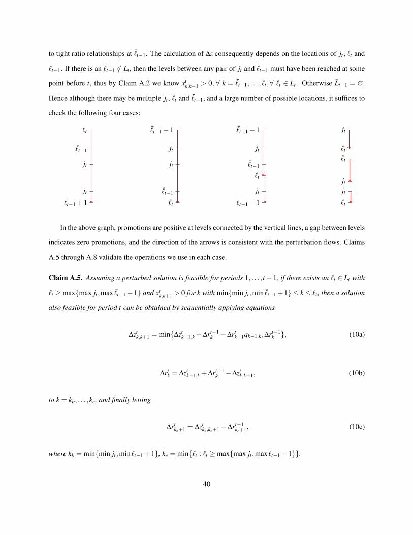
to tight ratio relationships at ¯t−1. The calculation of ∆z consequently depends on the locations of jt , `t and
¯t−1. If there is an ¯t−1 /∈ Lt , then the levels between any pair of jt and ¯t−1 must have been reached at some
point before t, thus by Claim A.2 we know xtk,k+1 > 0, ∀ k = ¯t−1, . . . , `t ,∀ `t ∈ Lt . Otherwise Lt−1 = ∅.
Hence although there may be multiple jt , `t and ¯t−1, and a large number of possible locations, it suffices to
check the following four cases:
`t
¯t−1
jt
jt¯t−1 +1
¯t−1−1
jt
jt
¯t−1
`t
¯t−1−1
jt
¯t−1
`t
jt¯t−1 +1
jt
`t
`t
jtjt`t
In the above graph, promotions are positive at levels connected by the vertical lines, a gap between levels
indicates zero promotions, and the direction of the arrows is consistent with the perturbation flows. Claims
A.5 through A.8 validate the operations we use in each case.
Claim A.5. Assuming a perturbed solution is feasible for periods 1, . . . , t−1, if there exists an `t ∈ Lt with
`t ≥max{max jt ,max ¯t−1 +1} and xtk,k+1 > 0 for k with min{min jt ,min ¯t−1 +1} ≤ k≤ `t , then a solution
also feasible for period t can be obtained by sequentially applying equations
∆ztk,k+1 = min{∆zt
k−1,k +∆rt−1k −∆rt
k−1qk−1,k,∆rt−1k }, (10a)
∆rtk = ∆zt
k−1,k +∆rt−1k −∆zt
k,k+1, (10b)
to k = kb, . . . ,ke, and finally letting
∆rtke+1 = ∆zt
ke,ke+1 +∆rt−1ke+1, (10c)
where kb = min{min jt ,min ¯t−1 +1}, ke = min{`t : `t ≥max{max jt ,max ¯t−1 +1}}.
40

Proof. We can choose the smallest such `t as a common level for the perturbation driven by all jt and ¯t−1
to stop in period t. To fix potential infeasibility caused by full promotions or tight ratio relationships, it
is reasonable to decrease the promotions at these levels and update employment accordingly. The level to
start such operations should of course be min{min jt , min ¯t−1 + 1}. The decreasing effect will finally be
conveyed to the `t we choose.
We consider level k to determine ∆ztk,k+1. Since ∆rt−1
k , ∆rtk−1, and ∆zt
k−1,k (in particular, ∆ztkb−1,kb
= 0)
are all known as we reach node (k, t), we can solve
∆zt
k−1,k +∆rt−1k = ∆zt
k,k+1 +∆rtk
∆rtk ≥ ∆rt
k−1qk−1,k
∆ztk,k+1 ≤ ∆rt−1
k
,
and choose the largest possible ∆ztk,k+1 (so that |∆zt
k,k+1| is as small as possible), which yields (10a). The
three constraints above represent flow conservation, ratio relationships, and promotion bounds respectively.
∆rtk can then be determined via flow conservation, i.e. (10b). (10c) is a result of stopping perturbation at
ke. �
Claim A.6. Assuming a perturbed solution is feasible for periods 1, . . . , t−1, if there exists an `t ∈ Lt with
`t ≤min{min jt ,min ¯t−1−1} and xtk,k+1 > 0 for k with `t ≤ k≤max{max jt ,max ¯t−1−1}, then a solution
also feasible for period t can be obtained by sequentially applying equations
∆ztk,k+1 = min{∆zt
k+1,k+2 +∆rtk+2/qk+1,k+2−∆rt−1
k+1,∆rt−1k }, (11a)
∆rtk+1 = ∆zt
k,k+1 +∆rt−1k+1−∆zt
k+1,k+2, (11b)
to k = kb, . . . ,ke, and finally letting
∆rtke= ∆rt−1
ke−∆zt
ke,ke+1, (11c)
41

where kb = max{max jt ,max ¯t−1−1}, ke = max{`t : `t ≤min{min jt ,min ¯t−1−1}}.
Proof. We can choose the largest such `t as a common level for the perturbation driven by all jt and ¯t−1
to stop in period t. Again we fix potential infeasibility by decreasing promotions. But unlike the previous
claim, we operate in a top-down fashion since the perturbation is expected to end at the `t ∈ Lt we choose.
We consider level k+ 1 to determine ∆ztk,k+1. Since ∆rt−1
k+1, ∆rt−1k , ∆rt
k+2, and ∆ztk+1,k+2 (in particular,
∆ztkb+1,kb+2 = 0) are all known as we reach node (k+1, t), we can solve
∆zt
k,k+1 +∆rt−1k+1 = ∆zt
k+1,k+2 +∆rtk+1
∆rtk+1 ≤ ∆rt
k+2/qk+1,k+2
∆ztk,k+1 ≤ ∆rt−1
k
,
and choose the largest possible ∆ztk,k+1, which yields (11a). ∆r can then be determined via flow conservation,
i.e. (11b) and (11c). �
Claim A.7. Assuming a perturbed solution is feasible for periods 1, . . . , t−1, if there exists an `t ∈ Lt with
min{min jt ,min ¯t−1+1} ≤ `t ≤max{max jt ,max ¯t−1−1} and xtk,k+1 > 0 for k with min{min jt ,min ¯t−1+
1} ≤ k ≤ max{max jt ,max ¯t−1− 1}, then a solution also feasible for period t can be obtained by sequen-
tially applying equations (10) to levels min{min jt ,min ¯t−1 + 1} ≤ k ≤ `t − 1, equations (11) to levels
`t +1≤ k ≤max{max jt ,max ¯t−1−1}, and finally letting
∆zt`t ,`t+1 =
min{∆rt−1`t
+∆zt`t−1,`t
−∆rt`t−1q`t−1,`t , ∆zt
`t+1,`t+2 +∆rt`t+2/q`t+1,`t+2−∆rt−1
`t+1, ∆rt−1`t}
(12a)
∆rt`t= ∆zt
`t−1,`t+∆rt−1
`t−∆zt
`t ,`t+1 (12b)
∆rt`t+1 = ∆zt
`t ,`t+1 +∆rt−1`t+1−∆zt
`t+1,`t+2. (12c)
Proof. This is a hybrid of the previous two claims. By a similar analysis the perturbation should only
42

cover levels from min{min jt ,min ¯t−1 + 1} to max{max jt ,max ¯t−1− 1}. We can treat any such `t as a
breakpoint above which Claim A.6 applies and below which Claim A.5 applies. It only remains to perturb
level `t itself. To guarantee feasibility we can choose the minimum of the values provided by Claims A.5
and A.6 to determine ∆zt`t ,`t+1, and ∆rt
`t+1 and ∆rt`t
can then be calculated by flow conservation. This yields
(12). �
Claim A.8. Assuming a perturbed solution is feasible for periods 1, . . . , t−1, if there are zero promotions
between successive levels `t , . . . , jt or jt , . . . , `t , then a solution also feasible for period t can be obtained
by applying (10) to each succession `t , . . . , jt or (11) to each succession jt , . . . , `t , as long as the jt values
partition Jt .
Proof. By Claim A.2 there is no ¯t−1 and so we only consider the impact of full promotions at jt . The
applicability of the claims follows immediately from the fact that each succession here is an instance of
Claim A.5 or A.6.
We need to ensure, though, that each jt is included in exactly one succession. Starting from max jt , if
there exists some `t with `t ≥max jt and xtk,k+1 > 0 for k with max jt ≤ k ≤ `t , there may be a lower jt that
satisfies this condition as well; hence we can decrease promotions from the lowest such jt to any such `t ,
and use the formulas from Claim A.5 to determine ∆ztk,k+1 and ∆rt
k. Otherwise, by Claims A.3 and A.4 there
must exist some `t with `t < max jt and xtk,k+1 > 0 for k with `t ≤ k≤max jt , and so we can use the formulas
from Claim A.6 to determine ∆ztk,k+1 and ∆rt
k+1 until reaching the highest such `t . After either case is done,
we can move downwards to the next jt that has not been visited, and apply the same argument again. This
process goes on until reaching min jt . �
We now state our perturbation procedure as Procedure 2. Note that if in some period we find xtk+1,k+2 <
pst−1k+1 for each perturbed level k (including when Jt = Lt−1 =∅), the procedure can end in this period, and
from then on the perturbed solution will remain the same as the initial solution; otherwise, the procedure
will iterate forward infinitely but converge to a new feasible solution. Claim A.9 justifies the lower cost of
the final perturbed solution.
Claim A.9. Procedure 2 modifies the given solution by adding to it a series of negative cost cycles or infinite
paths in the time-space network.
43

Proof. Except for the possible end period, all the perturbations are initiated by decreasing the z values. Pick
any node (k, t) with negative ∆r flows in the perturbation network. Each time we conduct an operation as in
Claims A.5 to A.8, by flow conservation ∆rtk is passed to either ∆rt−1
k or ∆ztk−1,k, resulting in a left arc and a
downward arc, respectively. As this propagates, two cases may occur.
Case 1: We reach some `t (t ≤ t) where the flow turns right, then follows a right-down-right pattern, and
finally turns upwards at the perturbation’s end period. This constitutes a counterclockwise cycle as
described in Claim A.1.
Case 2: The flow may continue shifting in a right-down-right pattern perpetually, which constitutes a coun-
terclockwise infinite path as described in Claim A.1. �
Procedure 2 Perturbation when n≥ 3 and pk = pk+1,∀ k = 1, . . . ,n−11: ∆r1
m+1 =−∆r1m = ∆z1
m,m+1 =−ε , J1 = L1 = {m}, L0 =∅, t = 2,ep = 02: while ep = 0 do3: if xt
k+1,k+2 < pst−1k+1 for every perturbed level k then
4: ep = 15: else6: Run Procedure 1 to identify Jt , Lt , and Lt−17: if Claim A.5 is applicable then8: Perturb according to Claim A.59: else if Claim A.6 is applicable then
10: Perturb according to Claim A.611: else if Claim A.7 is applicable then12: Perturb according to Claim A.713: else14: Perturb according to Claim A.815: end if16: Update ∆x,∆s,x,s17: t = t +118: end if19: end while20: for perturbed levels k in increasing order do21: ∆zt
k,k+1 = ∆rt−1k +∆zt
k−1,k22: Update ∆x,∆s,x,s23: end for
44

A.4 A technical note on the perturbation amount ε
We have constructed perturbation operations that are feasible for small enough ε . To obtain a valid perturbed
solution, however, we need to guarantee that ε > 0. Because the perturbation may range over infinitely many
periods, it could be that the required ε eventually converges to zero. We next argue why this is not the case.
If the perturbation ends in some period, it essentially works in finite dimensions and thus ε > 0. On the
other hand, if the procedure iterates infinitely, ε depends on the x and s values. In particular, the values of the
training variables, promotion variables, and slack between consecutive levels matter since we are decreasing
them. To eliminate the possibility of ε converging to zero, it suffices to bound those values from below
wherever they are perturbed.
When n = 2, the proof of (4b) reduces the promotion in period 1 and increases it in later periods. The
increments depend on the reduction in period 1 and so depend on how much we can decrease there, which
clearly is positive. In the proof of (4a), ε depends on st+11 −dt+1 if xt+1
1,2 = p1st1, and p1st
1−xt+11,2 if st+1
1 = dt+1.
In the former case, st+11 −dt+1 =
p2st2+p1st
1q1,2
−dt+1 ≥ (pmin +pminqmax
)dt−dt+1 ≥ pmindt , which is bounded away
from zero since dt ≥ d1 > 0. In the latter case, the perturbation ends in period t + 1 so the perturbation is
finite.
Now consider when n ≥ 3. Recall that in all the cases considered for perturbation, we perturb levels
between jt and `t , or ¯t−1 and `t , or both. For any level k with `t ≤ k ≤ jt , the proof of Claim A.4 actually
provides a lower bound independent of t, i.e. xt+1k,k+1 > pqk+1, jt s
tk+1 ≥ pq1, jt d1. Furthermore, if we redefine
g = min{i : xt+1i,i+1 ≤C, jt +1≤ i≤ n}, where C > 0 can be any constant less than mint ′=1,...,t{pst ′
i } for each
i (such as C = pq1,nd1), the bound still holds, and hence the x variables at levels k with jt ≤ k ≤ `t are also
bounded below by a constant independent of t.
The same trick can be applied to any level k between `t and ¯t−1, i.e. the lower bounds on the x variables
in Claim A.2 can be strengthened from zero to the same constant C above. Finally, Claim A.3 is still correct
for xt+1g,g+1 ≤C as long as C < pqn−1
max d1. This enables us to use a g that still satisfies the properties in both
claims as the level starting from which a search of `t is conducted in Procedure 1.
Since the proofs of the claims only utilize the linear relationships between s and x, we can obtain similar
bounds for the slack between consecutive s variables. All the lower bounds depend only on d1 and fixed
parameters like n, p and q. It follows that the ε in the infinite case is indeed positive.
45

B Proof of Theorem 3.3
We will construct a one-period lookahead policy based on Lemmas 3.1 and 3.2, and then demonstrate that
the resulting solution is unique.
B.1 A one-period lookahead policy
The notation we use is summarized below:
• Bti,i+1: upper promotion bound for level i in period t.
• I: a list of levels where promotion bounds would be violated if hiring were not allowed.
Claim B.1. Consider a subsystem consisting of levels from j to k+1, 0≤ j≤ k≤ n−1 in period t. Assume
st−1i , i = j, . . . ,k+ 1 and st
j are known. If p j+1st−1j+1 < q j, j+1st
j and pi+1st−1i+1 ≤ qi,i+1 pist−1
i , i = j+ 1, . . . ,k,
then the unique solution to the following equations provides a solution that satisfies promotion bounds at
levels in I:
p j+1st−1j+1 + xt
j, j+1− xtj+1, j+2 + xt
j+1 = q j, j+1(stj− xt
j, j+1) (13a)
pi+1st−1i+1 + xt
i,i+1− xti+1,i+2 + xt
i+1 = qi,i+1(pist−1i + xt
i−1,i− xti,i+1 + xt
i),
i = j+1, . . . ,k−1(13b)
pk+1st−1k+1 + xt
k,k+1 + xtk+1 = qk,k+1(pkst−1
k + xtk−1,k− xt
k,k+1 + xtk), (13c)
where xti = 0 if i /∈ I and xt
i,i+1 = Bti,i+1 if i ∈ I.
Proof. Clearly any solution to the above linear system satisfies promotion bounds at any i∈ I. Nonnegativity
of the x variables is guaranteed by the deficiency of staff at level j and the tight ratio relationships (with
respect to retention from period t− 1) at levels j, . . . ,k. For a specific solution x, a policy can be obtained
46

by letting
sti =
st
i− xti,i+1, i = j
pist−1i + xt
i−1,i− xti,i+1 + xt
i, i = j+1, . . . ,k
pist−1i + xt
i−1,i + xti, i = k+1
. (14)
Let the coefficient matrix be such that column ` (`= 1, . . . ,k− j+1) records the coefficients of xtj+`−1, j+`
if j+ `−1 /∈ I and xtj+` otherwise. The elements are
am` =
−q j+`, j+`+1, m = `+1
1 if j+ `−1 ∈ I and 1+q j+`−1, j+` otherwise, m = `
0 if j+ `−1 ∈ I and −1 otherwise, m = `−1
0, otherwise
.
Define Dm (m = 1, . . . ,k− j+1) as the determinant of the submatrix composed of the first m rows and
the first m columns. For m≥ 3, we have the recursion
Dm =
Dm−1, j+m−1 ∈ I
(1+qm+ j−1,m+ j)Dm−1−qm+ j−1,m+ jDm−2, otherwise.
By induction we know Dk− j+1 ≥ Dk− j ≥ . . .≥ D1 > 0, and hence the solution is unique. �
We now construct a feasible one-period lookahead policy by solving subproblems composed of levels
1, . . . ,k+1 sequentially until k = n−1. During each loop, we first check if the resulting solution is feasible
without promotion at level k, if yes then we are done. Otherwise, we try to get a solution which uses only
promotions, i.e. solve (13) with I = ∅. If this happens to be feasible, then we update the st and xt values
and exit; otherwise we calculate a feasible solution by allowing hiring, i.e. solve (13) with I 6=∅. For each
k, we keep iterating these steps for subproblems composed of levels j, . . . ,k+ 1 so that we can stop at the
highest j and the lower levels are not affected. When determining promotion and hiring, we force the ratio
constraints to be tight so that we use the smallest possible xt . In other words, we promote and hire only if
47

necessary. A formal statement is described in Procedure 3.
Procedure 3 A one-period lookahead policy
1: sti = dt if i = 0 and pist−1
i if i≥ 1, Bt0,1 = 0 if t = 1 and ∞ if t ≥ 2, Bt
i,i+1 = pist−1i , i = 1, . . . ,n−1
2: k = 03: while k ≤ n−1 do4: j = k5: while j ≥ 0 and st
j+1 < q j, j+1stj do
6: I =∅7: Bt
j, j+1 = Btj, j+1− xt
j, j+18: Solve (13)9: I = {i : xt
i,i+1 > Bti,i+1, j ≤ i≤ k}
10: if I 6=∅ then11: while I is changed do12: Solve (13)13: Update I14: end while15: end if16: Update s with (14)17: j = j−118: end while19: k = k+120: end while
We end this section with two comments. First, the procedure is applicable to both n = 2 and n ≥ 3.
Second, once i enters I at some iteration, it will be there forever: The first time i enters I, xti,i+1 must be
decreased (from infeasibility) to full promotion and so sti must be increased in the next iteration (which
is true since the only possibility for sti not to be increased is then to decrease xt
i or xti−1,i, but this would
induce infeasibility between sti and lower levels). To further satisfy the ratio relationships at levels i to k,
st`+1(i ≤ ` ≤ k) cannot be decreased either, which in turn forces the promotions at these levels to be full if
they were. This implies the procedure terminates.
B.2 Optimality of the one-period lookahead policy
Claim B.2. Recursively applying Procedure 3 yields the unique solution that satisfies Lemmas 3.1 and 3.2.
Proof. Clearly the solution satisfies the lemmas. Suppose there are multiple feasible solutions for which the
lemmas hold. We compare an arbitrary one of them, say (u,y), with (s,x) obtained from Procedure 3. By
Lemma 3.1 ytk+1 > 0 only if yt
k,k+1 = pkut−1k . Start from the earliest period, say t, where there is a difference
48

between xt and yt . Pick the lowest different level, say i. We have stk = ut
k,∀ k≤ i−1, and st ′ = ut ′ ,∀ t ′≤ t−1.
We first note that yti,i+1 < xt
i,i+1 or yti < xt
i cannot be true; otherwise we should be able to obtain a smaller
xt as Procedure 3 finishes since a feasible solution must satisfy the ratio and bound constraints at every level.
We next show that yti,i+1 > xt
i,i+1 or yti > xt
i cannot be true, either. Since (u,y) is feasible, by (1e)
yti,i+1 > xt
i,i+1 or yti > xt
i implies utk > st
k for some k ≥ i, so there is over promotion/hiring and the lemmas
must be violated somewhere in (u,y). �
C Extended model used in the computational examples
We modified (1) for our computational examples as follows. Let:
• T ≥ 1: Length of planning horizon.
• L≥ 1: Length of the training program.
• a: Age of the student or worker, al ≤ a≤ au.
• p0,i ∈ (0,1): Per-period rate of continuing education for students in school year i = 1, . . . ,L− 1, or
per-period rate of graduating and going to the workforce for students in school year i = L.
• pk,a ∈ (0,1): Per-period retention rate of workers of age a = al, . . . ,au that stay in the system at level
k = 0, . . . ,n from one period to the next.
• mk,a: The age distribution of students (k = 0) or workers (k = 1, . . . ,n) of age a = al, . . . ,au.
• st0,i,a: Students of age a = al, . . . ,au in school year i = 1, . . . ,L at end of period t = 1, . . . ,T .
• stk,a: Workers of age a = al, . . . ,au in level k = 1, . . . ,n at end of period t = 1, . . . ,T .
Our modified problem has the following formulation.
min C(s,x) =T
∑t=1
γt−1( n
∑k=0
ckxtk +
n−1
∑k=1
ck,k+1xtk,k+1 +
n
∑k=1
hk
au
∑a=al
stk,a
)s.t.
au
∑a=al
st1,a ≥ dt , ∀ t = 1, . . . ,T
49

au
∑a=al
stk+1,a−qk,k+1
au
∑a=al
stk,a ≥ 0, ∀ k = 1, . . . ,n−1, ∀ t = 1, . . . ,T
st0,1,a−m0,axt
0 = 0, ∀ a = al, . . . ,au, ∀ t = 1, . . . ,T
st0,i,a− p0,i−1st−1
0,i−1,a−1 = 0, ∀ i = 2, . . . ,L ∀ a = al +1, . . . ,au−1, ∀ t = 1, . . . ,T
st0,i,au− p0,i−1(st−1
0,i−1,au+ st−1
0,i−1,au−1) = 0, ∀ i = 2, . . . ,L, ∀ t = 1, . . . ,T
st1,a− p1,a−1st−1
1,a−1−m1,axt1− p0,Lst−1
0,L,a−1 +m2,axt1,2 = 0,
∀ a = al +1, . . . ,au−1, ∀ t = 1, . . . ,T
st1,au− p1,aust−1
1,au− p1,au−1st−1
1,au−1−m1,auxt1− p0,L(st−1
0,L,au+ st−1
0,L,au−1)
+m2,axt1,2 = 0, ∀ t = 1, . . . ,T
pk,a−1st−1k,a−1− st
k,a +mk,axtk−1,k−mk+1,axt
k,k+1 +mk,axtk = 0, ∀ k = 2 . . . ,n−1,
∀ a = al +1, . . . ,au−1, ∀ t = 1, . . . ,T
pk,au−1st−1k,au−1 + pk,aust−1
k,au− st
k,au+mk,auxt
k−1,k−mk+1,auxtk,k+1 +mk,auxt
k = 0,
∀ k = 2 . . . ,n−1, ∀ t = 1, . . . ,T
pn,a−1st−1n,a−1 +mn,a(xt
n−1,n + xtn)− st
n,a = 0, ∀ a = al +1, . . . ,au−1,
∀ t = 1, . . . ,T
pn,au−1st−1n,au−1 + pn,aust−1
n,au+mn,au(x
tn−1,n + xt
n)− stn,au
= 0, ∀ t = 1, . . . ,T
pk,a−1st−1k,a−1−mk+1,axt
k,k+1 ≥ 0, ∀ k = 1, . . . ,n−1,
∀ a = al +1, . . . ,au, ∀ t = 1, . . . ,T
st0,i,a = 0, ∀ i = 2, . . . ,L ∀ a = al, . . . ,al + i−2, ∀ t = 1, . . . ,T
stk,a = 0, ∀ k = 2, . . . ,n−1, ∀ a = al, . . . ,al + k+L−2, ∀ t = 1, . . . ,T
xt ,st ≥ 0, ∀ t = 1, . . . ,T
50