Strain localization and shear banding in ductile materials

N. Bordignon, A. Piccolroaz, F. Dal Corso and D. Bigoni

DICAM, University of Trento, Italy

Abstract

A model of a shear band as a zero-thickness nonlinear interface is proposed and tested usingfinite element simulations. An imperfection approach is used in this model where a shear band,that is assumed to lie in a ductile matrix material (obeying von Mises plasticity with linearhardening), is present from the beginning of loading and is considered to be a zone in whichyielding occurs before the rest of the matrix. This approach is contrasted with a perturbativeapproach, developed for a J2-deformation theory material, in which the shear band is modelledto emerge at a certain stage of a uniform deformation. Both approaches concur in showing thatthe shear bands (differently from cracks) propagate rectilinearly under shear loading and thata strong stress concentration should be expected to be present at the tip of the shear band, twokey features in the understanding of failure mechanisms of ductile materials.

Keywords:

1 Introduction

When a ductile material is brought to an extreme strain state through a uniform loading process,the deformation may start to localize into thin and planar bands, often arranged in regular latticepatterns. This phenomenon is quite common and occurs in many materials over a broad range ofscales: from the kilometric scale in the earth crust (Kirby, 1985), down to the nanoscale in metallicglass (Yang, 2005), see the examples reported in Fig. 1.

After localization, unloading typically1 occurs in the material outside the bands, while strainquickly evolves inside, possibly leading to final fracture (as in the examples shown in Fig. 2, wherethe crack lattice is the signature of the initial shear band network) or to a progressive accumulationof deformation bands (as for instance in the case of the drinking straws, or of the iron meteorite, orof the uPVC sample shown in Fig. 1, or in the well-known case of granular materials, where fractureis usually absent and localization bands are made up of material at a different relative density, Gajoet al. 2004).

It follows from the above discussion that as strain localization represents a prelude to failure ofductile materials, its mechanical understanding paves the way to the innovative use of materials inextreme mechanical conditions. Although shear bands have been the subject of an intense research

1 For granular materials, there are cases in which unloading occurs inside the shear band, as shown by Gajo et al.(2004).

1

arX

iv:1

501.

0602

4v1

[co

nd-m

at.m

trl-

sci]

24

Jan

2015

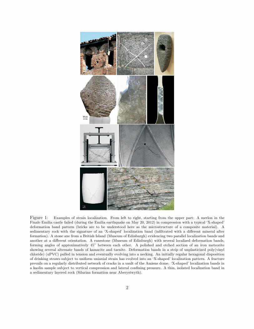
Figure 1: Examples of strain localization. From left to right, starting from the upper part: A merlon in theFinale Emilia castle failed (during the Emilia earthquake on May 20, 2012) in compression with a typical ‘X-shaped’deformation band pattern (bricks are to be understood here as the microstructure of a composite material). Asedimentary rock with the signature of an ‘X-shaped’ localization band (infiltrated with a different mineral afterformation). A stone axe from a British Island (Museum of Edinburgh) evidencing two parallel localization bands andanother at a different orientation. A runestone (Museum of Edinburgh) with several localized deformation bands,forming angles of approximatively 45◦ between each other. A polished and etched section of an iron meteoriteshowing several alternate bands of kamacite and taenite. Deformation bands in a strip of unplasticized poly(vinylchloride) (uPVC) pulled in tension and eventually evolving into a necking. An initially regular hexagonal dispositionof drinking straws subject to uniform uniaxial strain has evolved into an ‘X-shaped’ localization pattern. A fractureprevails on a regularly distributed network of cracks in a vault of the Amiens dome. ‘X-shaped’ localization bands ina kaolin sample subject to vertical compression and lateral confining pressure. A thin, isolated localization band ina sedimentary layered rock (Silurian formation near Aberystwyth).

2

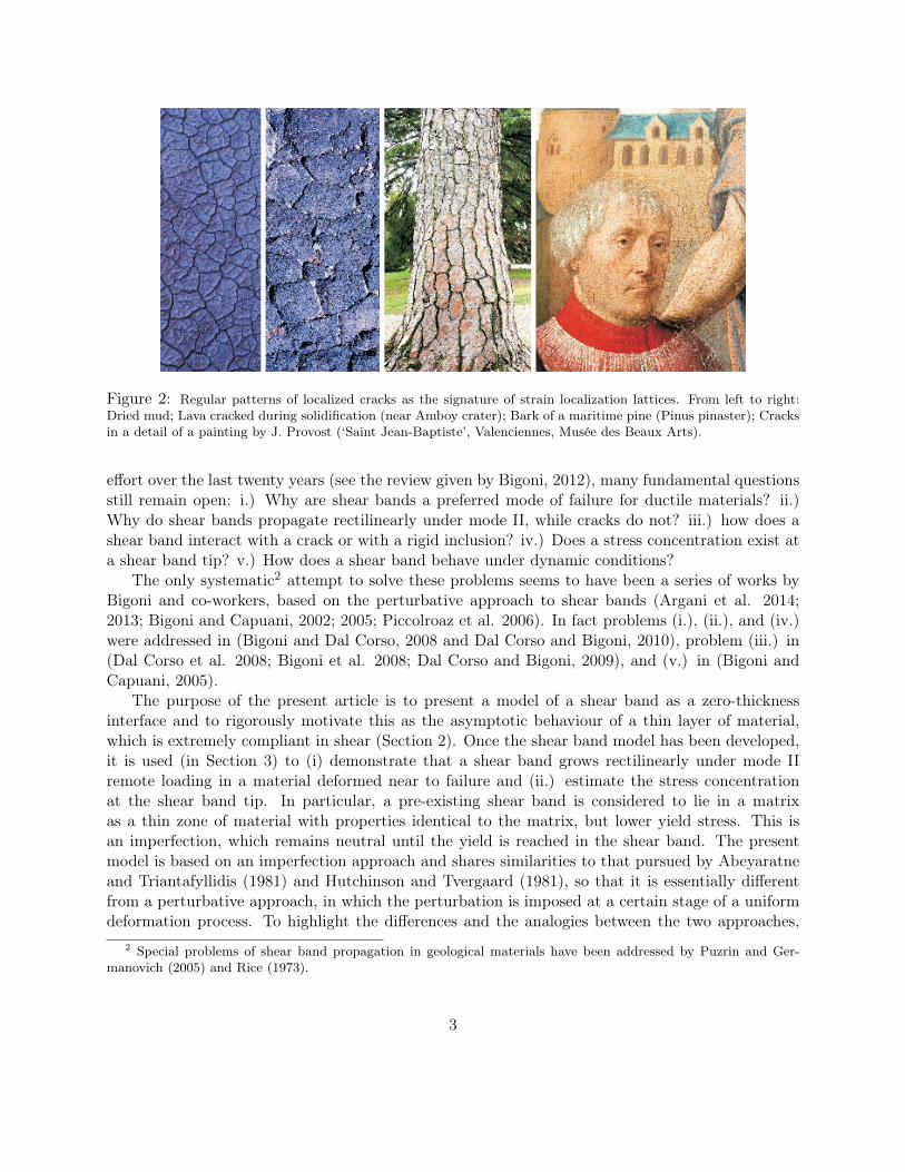
Figure 2: Regular patterns of localized cracks as the signature of strain localization lattices. From left to right:Dried mud; Lava cracked during solidification (near Amboy crater); Bark of a maritime pine (Pinus pinaster); Cracksin a detail of a painting by J. Provost (‘Saint Jean-Baptiste’, Valenciennes, Musée des Beaux Arts).

effort over the last twenty years (see the review given by Bigoni, 2012), many fundamental questionsstill remain open: i.) Why are shear bands a preferred mode of failure for ductile materials? ii.)Why do shear bands propagate rectilinearly under mode II, while cracks do not? iii.) how does ashear band interact with a crack or with a rigid inclusion? iv.) Does a stress concentration exist ata shear band tip? v.) How does a shear band behave under dynamic conditions?

The only systematic2 attempt to solve these problems seems to have been a series of works byBigoni and co-workers, based on the perturbative approach to shear bands (Argani et al. 2014;2013; Bigoni and Capuani, 2002; 2005; Piccolroaz et al. 2006). In fact problems (i.), (ii.), and (iv.)were addressed in (Bigoni and Dal Corso, 2008 and Dal Corso and Bigoni, 2010), problem (iii.) in(Dal Corso et al. 2008; Bigoni et al. 2008; Dal Corso and Bigoni, 2009), and (v.) in (Bigoni andCapuani, 2005).

The purpose of the present article is to present a model of a shear band as a zero-thicknessinterface and to rigorously motivate this as the asymptotic behaviour of a thin layer of material,which is extremely compliant in shear (Section 2). Once the shear band model has been developed,it is used (in Section 3) to (i) demonstrate that a shear band grows rectilinearly under mode IIremote loading in a material deformed near to failure and (ii.) estimate the stress concentrationat the shear band tip. In particular, a pre-existing shear band is considered to lie in a matrixas a thin zone of material with properties identical to the matrix, but lower yield stress. This isan imperfection, which remains neutral until the yield is reached in the shear band. The presentmodel is based on an imperfection approach and shares similarities to that pursued by Abeyaratneand Triantafyllidis (1981) and Hutchinson and Tvergaard (1981), so that it is essentially differentfrom a perturbative approach, in which the perturbation is imposed at a certain stage of a uniformdeformation process. To highlight the differences and the analogies between the two approaches,

2 Special problems of shear band propagation in geological materials have been addressed by Puzrin and Ger-manovich (2005) and Rice (1973).

3

the incremental strain field induced by the emergence of a shear band of finite length (modelled as asliding surface) is determined for a J2-deformation theory material and compared with finite elementsimulations in which the shear band is modelled as a zero-thickness layer of compliant material.

2 Asymptotic model for a thin layer of highly compliant materialembedded in a solid

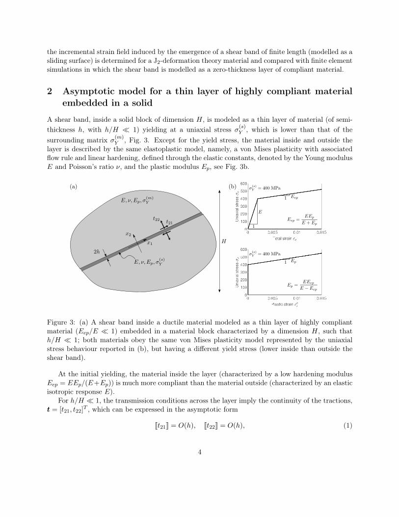
A shear band, inside a solid block of dimension H, is modeled as a thin layer of material (of semi-thickness h, with h/H � 1) yielding at a uniaxial stress σ(s)Y , which is lower than that of thesurrounding matrix σ(m)

Y , Fig. 3. Except for the yield stress, the material inside and outside thelayer is described by the same elastoplastic model, namely, a von Mises plasticity with associatedflow rule and linear hardening, defined through the elastic constants, denoted by the Young modulusE and Poisson’s ratio ν, and the plastic modulus Ep, see Fig. 3b.

Figure 3: (a) A shear band inside a ductile material modeled as a thin layer of highly compliantmaterial (Eep/E � 1) embedded in a material block characterized by a dimension H, such thath/H � 1; both materials obey the same von Mises plasticity model represented by the uniaxialstress behaviour reported in (b), but having a different yield stress (lower inside than outside theshear band).

At the initial yielding, the material inside the layer (characterized by a low hardening modulusEep = EEp/(E+Ep)) is much more compliant than the material outside (characterized by an elasticisotropic response E).

For h/H � 1, the transmission conditions across the layer imply the continuity of the tractions,t = [t21, t22]

T , which can be expressed in the asymptotic form

Jt21K = O(h), Jt22K = O(h), (1)

4

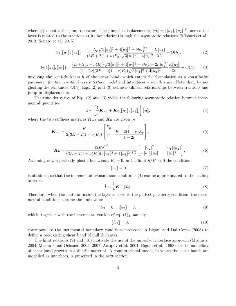
where J·K denotes the jump operator. The jump in displacements, JuK = [Ju1K, Ju2K]T , across thelayer is related to the tractions at its boundaries through the asymptotic relations (Mishuris et al.,2013; Sonato et al., 2015)

t21(Ju1K, Ju2K) =Ep

√3Ju1K2 + 4Ju2K2 + 6hσ

(s)Y

(3E + 2(1 + ν)Ep)√

3Ju1K2 + 4Ju2K2EJu1K

2h+O(h), (2)

t22(Ju1K, Ju2K) =(E + 2(1− ν)Ep)

√3Ju1K2 + 4Ju2K2 + 8h(1− 2ν)σ

(s)Y

(1− 2ν)(3E + 2(1 + ν)Ep)√

3Ju1K2 + 4Ju2K2EJu2K

2h+O(h), (3)

involving the semi-thickness h of the shear band, which enters the formulation as a constitutiveparameter for the zero-thickness interface model and introduces a length scale. Note that, by ne-glecting the remainder O(h), Eqs. (2) and (3) define nonlinear relationships between tractions andjump in displacements.

The time derivative of Eqs. (2) and (3) yields the following asymptotic relation between incre-mental quantities

t ∼[

1

hK−1 + K0(Ju1K, Ju2K)

]JuK, (4)

where the two stiffness matrices K−1 and K0 are given by

K−1 =E

2(3E + 2(1 + ν)Ep)

Ep 0

0E + 2(1− ν)Ep

1− 2ν

, (5)

K0 =12Eσ

(s)Y

(3E + 2(1 + ν)Ep)(3Ju1K2 + 4Ju2K2)3/2

[Ju2K2 −Ju1KJu2K

−Ju1KJu2K Ju1K2

], (6)

Assuming now a perfectly plastic behaviour, Ep = 0, in the limit h/H → 0 the condition

Ju2K = 0 (7)

is obtained, so that the incremental transmission conditions (4) can be approximated to the leadingorder as

t ∼ 1

hK−1JuK. (8)

Therefore, when the material inside the layer is close to the perfect plasticity condition, the incre-mental conditions assume the limit value

t21 = 0, Ju2K = 0, (9)

which, together with the incremental version of eq. (1)2, namely,

Jt22K = 0, (10)

correspond to the incremental boundary conditions proposed in Bigoni and Dal Corso (2008) todefine a pre-existing shear band of null thickness.

The limit relations (9) and (10) motivate the use of the imperfect interface approach (Mishuris,2004; Mishuris and Ochsner, 2005; 2007; Antipov et al. 2001; Bigoni et al., 1998) for the modellingof shear band growth in a ductile material. A computational model, in which the shear bands aremodelled as interfaces, is presented in the next section.

5

3 Numerical simulations

Two-dimensional plane-strain finite element simulations are presented to show the effectiveness ofthe above-described asymptotic model for a thin and highly compliant layer in modelling a shearband embedded in a ductile material. Specifically, we will show that the model predicts rectilinearpropagation of a shear band under simple shear boundary conditions and it allows the investigationof the stress concentration at the shear band tip.

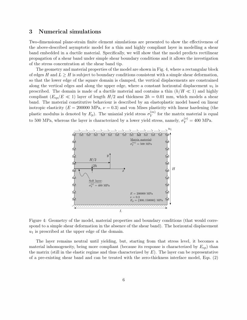
The geometry and material properties of the model are shown in Fig. 4, where a rectangular blockof edges H and L ≥ H is subject to boundary conditions consistent with a simple shear deformation,so that the lower edge of the square domain is clamped, the vertical displacements are constrainedalong the vertical edges and along the upper edge, where a constant horizontal displacement u1 isprescribed. The domain is made of a ductile material and contains a thin (h/H � 1) and highlycompliant (Eep/E � 1) layer of length H/2 and thickness 2h = 0.01 mm, which models a shearband. The material constitutive behaviour is described by an elastoplastic model based on linearisotropic elasticity (E = 200000 MPa, ν = 0.3) and von Mises plasticity with linear hardening (theplastic modulus is denoted by Ep). The uniaxial yield stress σ(m)

Y for the matrix material is equalto 500 MPa, whereas the layer is characterized by a lower yield stress, namely, σ(s)Y = 400 MPa.

Figure 4: Geometry of the model, material properties and boundary conditions (that would corre-spond to a simple shear deformation in the absence of the shear band). The horizontal displacementu1 is prescribed at the upper edge of the domain.

The layer remains neutral until yielding, but, starting from that stress level, it becomes amaterial inhomogeneity, being more compliant (because its response is characterized by Eep) thanthe matrix (still in the elastic regime and thus characterized by E). The layer can be representativeof a pre-existing shear band and can be treated with the zero-thickness interface model, Eqs. (2)

6

and (3). This zero-thickness interface was implemented in the ABAQUS finite element software3

through cohesive elements, equipped with the traction-separation laws, Eqs. (2) and (3), by meansof the user subroutine UMAT. An interface, embedded into the cohesive elements, is characterizedby two dimensions: a geometrical and a constitutive thickness. The latter, 2h, exactly correspondsto the constitutive thickness involved in the model for the interface (2) and (3), while the former,denoted by 2hg, is related to the mesh dimension in a way that the results become independentof this parameter, in the sense that a mesh refinement yields results converging to a well-definedsolution.

We consider two situations. In the first, we assume that the plastic modulus is Ep = 150000MPa (both inside and outside the shear band), so that the material is in a state far from a shearband instability (represented by loss of ellipticity of the tangent constitutive operator, occurringat Ep = 0) when at yield. In the second, we assume that the material is prone to a shear bandinstability, though still in the elliptic regime, so that Ep (both inside and outside the shear band) isselected to be ‘sufficiently small’, namely, Ep = 300 MPa. The pre-existing shear band is thereforeemployed as an imperfection triggering shear strain localization when the material is still inside theregion, but close to the boundary, of ellipticity.

3.1 Description of the numerical model

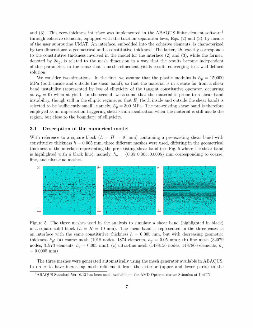
With reference to a square block (L = H = 10 mm) containing a pre-existing shear band withconstitutive thickness h = 0.005 mm, three different meshes were used, differing in the geometricalthickness of the interface representing the pre-existing shear band (see Fig. 5 where the shear bandis highlighted with a black line), namely, hg = {0.05; 0.005; 0.0005} mm corresponding to coarse,fine, and ultra-fine meshes.

Figure 5: The three meshes used in the analysis to simulate a shear band (highlighted in black)in a square solid block (L = H = 10 mm). The shear band is represented in the three cases asan interface with the same constitutive thickness h = 0.005 mm, but with decreasing geometricthickness hg; (a) coarse mesh (1918 nodes, 1874 elements, hg = 0.05 mm); (b) fine mesh (32079nodes, 31973 elements, hg = 0.005 mm); (c) ultra-fine mesh (1488156 nodes, 1487866 elements, hg= 0.0005 mm)

The three meshes were generated automatically using the mesh generator available in ABAQUS.In order to have increasing mesh refinement from the exterior (upper and lower parts) to the

3ABAQUS Standard Ver. 6.13 has been used, available on the AMD Opteron cluster Stimulus at UniTN.

7

interior (central part) of the domain, where the shear band is located, and to ensure the appropriateelement shape and size according to the geometrical thickness 2hg, the domain was partitioned intorectangular subdomains with increasing mesh seeding from the exterior to the interior. Afterwards,the meshes were generated by employing a free meshing technique with quadrilateral elements andthe advancing front algorithm.

The interface that models the shear band is discretized using 4-node two-dimensional cohesive el-ements (COH2D4), while the matrix material is modelled using 4-node bilinear, reduced integrationwith hourglass control (CPE4R).

It is important to note that the constitutive thickness used for traction-separation response isalways equal to the actual size of the shear band h = 0.005 mm, whereas the geometric thickness hg,defining the height of the cohesive elements, is different for the three different meshes. Consequently,all the three meshes used in the simulations correspond to the same problem in terms of both materialproperties and geometrical dimensions (although the geometric size of the interface is different), sothat the results have to be, and indeed will be shown to be, mesh independent.

3.2 Numerical results

Results (obtained using the fine mesh, Fig. 5b) in terms of the shear stress component σ12 at differentstages of a deformation process for the boundary value problem sketched in Fig. 4 are reported inFigs. 6 and 7.

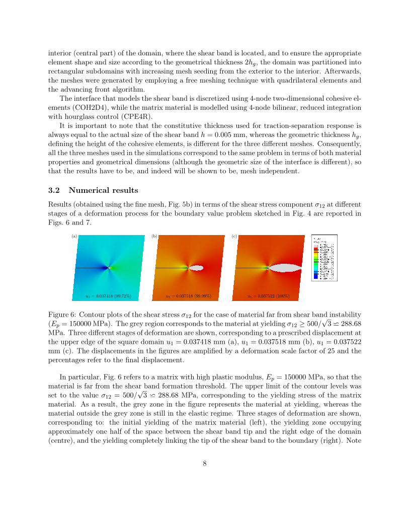
Figure 6: Contour plots of the shear stress σ12 for the case of material far from shear band instability(Ep = 150000 MPa). The grey region corresponds to the material at yielding σ12 ≥ 500/

√3 w 288.68

MPa. Three different stages of deformation are shown, corresponding to a prescribed displacement atthe upper edge of the square domain u1 = 0.037418 mm (a), u1 = 0.037518 mm (b), u1 = 0.037522mm (c). The displacements in the figures are amplified by a deformation scale factor of 25 and thepercentages refer to the final displacement.

In particular, Fig. 6 refers to a matrix with high plastic modulus, Ep = 150000 MPa, so that thematerial is far from the shear band formation threshold. The upper limit of the contour levels wasset to the value σ12 = 500/

√3 w 288.68 MPa, corresponding to the yielding stress of the matrix

material. As a result, the grey zone in the figure represents the material at yielding, whereas thematerial outside the grey zone is still in the elastic regime. Three stages of deformation are shown,corresponding to: the initial yielding of the matrix material (left), the yielding zone occupyingapproximately one half of the space between the shear band tip and the right edge of the domain(centre), and the yielding completely linking the tip of the shear band to the boundary (right). Note

8

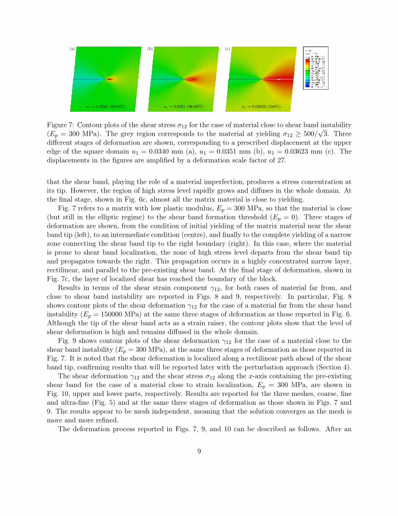
Figure 7: Contour plots of the shear stress σ12 for the case of material close to shear band instability(Ep = 300 MPa). The grey region corresponds to the material at yielding σ12 ≥ 500/

√3. Three

different stages of deformation are shown, corresponding to a prescribed displacement at the upperedge of the square domain u1 = 0.0340 mm (a), u1 = 0.0351 mm (b), u1 = 0.03623 mm (c). Thedisplacements in the figures are amplified by a deformation scale factor of 27.

that the shear band, playing the role of a material imperfection, produces a stress concentration atits tip. However, the region of high stress level rapidly grows and diffuses in the whole domain. Atthe final stage, shown in Fig. 6c, almost all the matrix material is close to yielding.

Fig. 7 refers to a matrix with low plastic modulus, Ep = 300 MPa, so that the material is close(but still in the elliptic regime) to the shear band formation threshold (Ep = 0). Three stages ofdeformation are shown, from the condition of initial yielding of the matrix material near the shearband tip (left), to an intermediate condition (centre), and finally to the complete yielding of a narrowzone connecting the shear band tip to the right boundary (right). In this case, where the materialis prone to shear band localization, the zone of high stress level departs from the shear band tipand propagates towards the right. This propagation occurs in a highly concentrated narrow layer,rectilinear, and parallel to the pre-existing shear band. At the final stage of deformation, shown inFig. 7c, the layer of localized shear has reached the boundary of the block.

Results in terms of the shear strain component γ12, for both cases of material far from, andclose to shear band instability are reported in Figs. 8 and 9, respectively. In particular, Fig. 8shows contour plots of the shear deformation γ12 for the case of a material far from the shear bandinstability (Ep = 150000 MPa) at the same three stages of deformation as those reported in Fig. 6.Although the tip of the shear band acts as a strain raiser, the contour plots show that the level ofshear deformation is high and remains diffused in the whole domain.

Fig. 9 shows contour plots of the shear deformation γ12 for the case of a material close to theshear band instability (Ep = 300 MPa), at the same three stages of deformation as those reported inFig. 7. It is noted that the shear deformation is localized along a rectilinear path ahead of the shearband tip, confirming results that will be reported later with the perturbation approach (Section 4).

The shear deformation γ12 and the shear stress σ12 along the x-axis containing the pre-existingshear band for the case of a material close to strain localization, Ep = 300 MPa, are shown inFig. 10, upper and lower parts, respectively. Results are reported for the three meshes, coarse, fineand ultra-fine (Fig. 5) and at the same three stages of deformation as those shown in Figs. 7 and9. The results appear to be mesh independent, meaning that the solution converges as the mesh ismore and more refined.

The deformation process reported in Figs. 7, 9, and 10 can be described as follows. After an

9

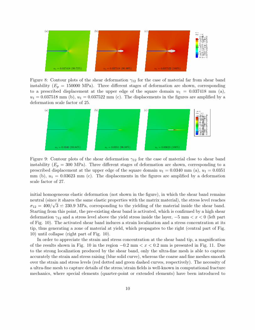
Figure 8: Contour plots of the shear deformation γ12 for the case of material far from shear bandinstability (Ep = 150000 MPa). Three different stages of deformation are shown, correspondingto a prescribed displacement at the upper edge of the square domain u1 = 0.037418 mm (a),u1 = 0.037518 mm (b), u1 = 0.037522 mm (c). The displacements in the figures are amplified by adeformation scale factor of 25.

Figure 9: Contour plots of the shear deformation γ12 for the case of material close to shear bandinstability (Ep = 300 MPa). Three different stages of deformation are shown, corresponding to aprescribed displacement at the upper edge of the square domain u1 = 0.0340 mm (a), u1 = 0.0351mm (b), u1 = 0.03623 mm (c). The displacements in the figures are amplified by a deformationscale factor of 27.

initial homogeneous elastic deformation (not shown in the figure), in which the shear band remainsneutral (since it shares the same elastic properties with the matrix material), the stress level reachesσ12 = 400/

√3 w 230.9 MPa, corresponding to the yielding of the material inside the shear band.

Starting from this point, the pre-existing shear band is activated, which is confirmed by a high sheardeformation γ12 and a stress level above the yield stress inside the layer, −5 mm < x < 0 (left partof Fig. 10). The activated shear band induces a strain localization and a stress concentration at itstip, thus generating a zone of material at yield, which propagates to the right (central part of Fig.10) until collapse (right part of Fig. 10).

In order to appreciate the strain and stress concentration at the shear band tip, a magnificationof the results shown in Fig. 10 in the region −0.2 mm < x < 0.2 mm is presented in Fig. 11. Dueto the strong localization produced by the shear band, only the ultra-fine mesh is able to captureaccurately the strain and stress raising (blue solid curve), whereas the coarse and fine meshes smoothover the strain and stress levels (red dotted and green dashed curves, respectively). The necessity ofa ultra-fine mesh to capture details of the stress/strain fields is well-known in computational fracturemechanics, where special elements (quarter-point or extended elements) have been introduced to

10

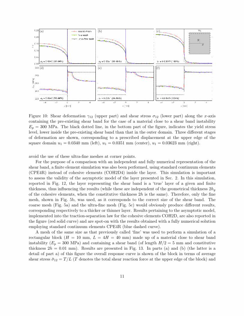
Figure 10: Shear deformation γ12 (upper part) and shear stress σ12 (lower part) along the x-axiscontaining the pre-existing shear band for the case of a material close to a shear band instabilityEp = 300 MPa. The black dotted line, in the bottom part of the figure, indicates the yield stresslevel, lower inside the pre-existing shear band than that in the outer domain. Three different stagesof deformation are shown, corresponding to a prescribed displacement at the upper edge of thesquare domain u1 = 0.0340 mm (left), u1 = 0.0351 mm (center), u1 = 0.03623 mm (right).

avoid the use of these ultra-fine meshes at corner points.For the purpose of a comparison with an independent and fully numerical representation of the

shear band, a finite element simulation was also been performed, using standard continuum elements(CPE4R) instead of cohesive elements (COH2D4) inside the layer. This simulation is importantto assess the validity of the asymptotic model of the layer presented in Sec. 2. In this simulation,reported in Fig. 12, the layer representing the shear band is a ‘true’ layer of a given and finitethickness, thus influencing the results (while these are independent of the geometrical thickness 2hgof the cohesive elements, when the constitutive thickness 2h is the same). Therefore, only the finemesh, shown in Fig. 5b, was used, as it corresponds to the correct size of the shear band. Thecoarse mesh (Fig. 5a) and the ultra-fine mesh (Fig. 5c) would obviously produce different results,corresponding respectively to a thicker or thinner layer. Results pertaining to the asymptotic model,implemented into the traction-separation law for the cohesive elements COH2D, are also reported inthe figure (red solid curve) and are spot-on with the results obtained with a fully numerical solutionemploying standard continuum elements CPE4R (blue dashed curve).

A mesh of the same size as that previously called ‘fine’ was used to perform a simulation of arectangular block (H = 10 mm, L = 4H = 40 mm) made up of a material close to shear bandinstability (Ep = 300 MPa) and containing a shear band (of length H/2 = 5 mm and constitutivethickness 2h = 0.01 mm). Results are presented in Fig. 13. In parts (a) and (b) (the latter is adetail of part a) of this figure the overall response curve is shown of the block in terms of averageshear stress σ12 = T/L (T denotes the total shear reaction force at the upper edge of the block) and

11

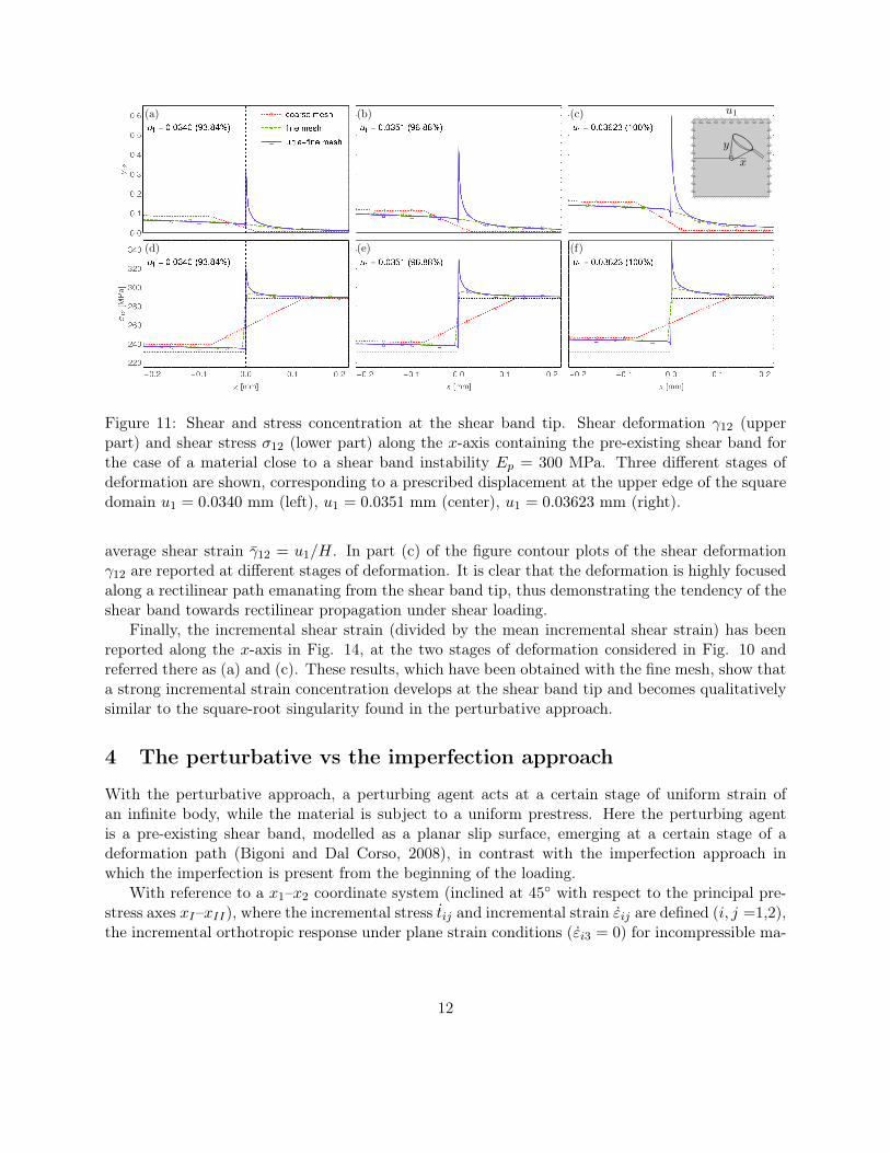
Figure 11: Shear and stress concentration at the shear band tip. Shear deformation γ12 (upperpart) and shear stress σ12 (lower part) along the x-axis containing the pre-existing shear band forthe case of a material close to a shear band instability Ep = 300 MPa. Three different stages ofdeformation are shown, corresponding to a prescribed displacement at the upper edge of the squaredomain u1 = 0.0340 mm (left), u1 = 0.0351 mm (center), u1 = 0.03623 mm (right).

average shear strain γ12 = u1/H. In part (c) of the figure contour plots of the shear deformationγ12 are reported at different stages of deformation. It is clear that the deformation is highly focusedalong a rectilinear path emanating from the shear band tip, thus demonstrating the tendency of theshear band towards rectilinear propagation under shear loading.

Finally, the incremental shear strain (divided by the mean incremental shear strain) has beenreported along the x-axis in Fig. 14, at the two stages of deformation considered in Fig. 10 andreferred there as (a) and (c). These results, which have been obtained with the fine mesh, show thata strong incremental strain concentration develops at the shear band tip and becomes qualitativelysimilar to the square-root singularity found in the perturbative approach.

4 The perturbative vs the imperfection approach

With the perturbative approach, a perturbing agent acts at a certain stage of uniform strain ofan infinite body, while the material is subject to a uniform prestress. Here the perturbing agentis a pre-existing shear band, modelled as a planar slip surface, emerging at a certain stage of adeformation path (Bigoni and Dal Corso, 2008), in contrast with the imperfection approach inwhich the imperfection is present from the beginning of the loading.

With reference to a x1–x2 coordinate system (inclined at 45◦ with respect to the principal pre-stress axes xI–xII), where the incremental stress tij and incremental strain εij are defined (i, j =1,2),the incremental orthotropic response under plane strain conditions (εi3 = 0) for incompressible ma-

12

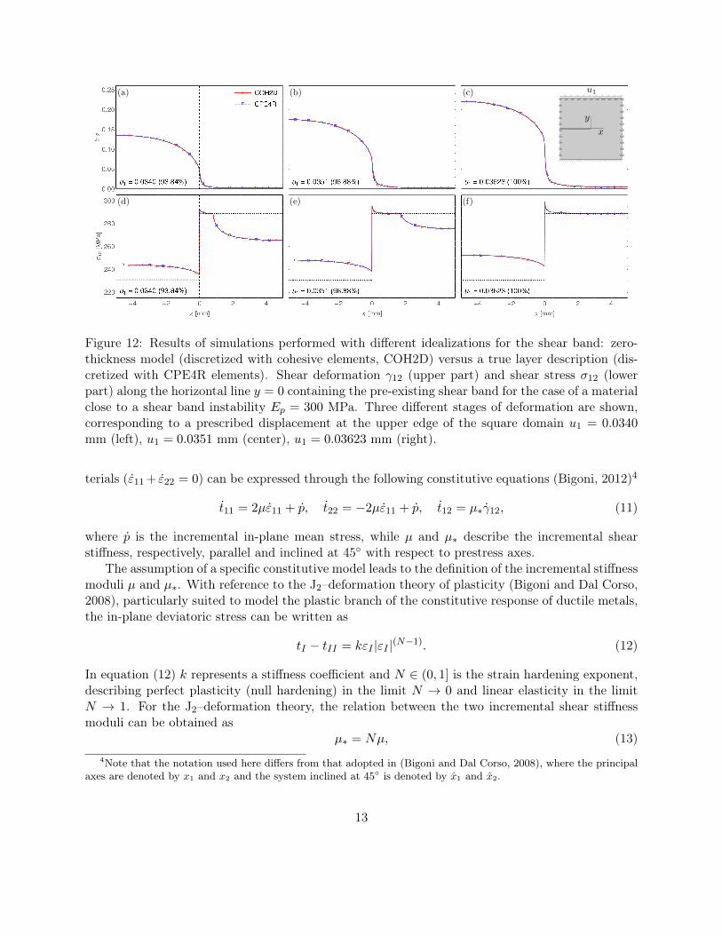
Figure 12: Results of simulations performed with different idealizations for the shear band: zero-thickness model (discretized with cohesive elements, COH2D) versus a true layer description (dis-cretized with CPE4R elements). Shear deformation γ12 (upper part) and shear stress σ12 (lowerpart) along the horizontal line y = 0 containing the pre-existing shear band for the case of a materialclose to a shear band instability Ep = 300 MPa. Three different stages of deformation are shown,corresponding to a prescribed displacement at the upper edge of the square domain u1 = 0.0340mm (left), u1 = 0.0351 mm (center), u1 = 0.03623 mm (right).

terials (ε11 + ε22 = 0) can be expressed through the following constitutive equations (Bigoni, 2012)4

t11 = 2µε11 + p, t22 = −2µε11 + p, t12 = µ∗γ12, (11)

where p is the incremental in-plane mean stress, while µ and µ∗ describe the incremental shearstiffness, respectively, parallel and inclined at 45◦ with respect to prestress axes.

The assumption of a specific constitutive model leads to the definition of the incremental stiffnessmoduli µ and µ∗. With reference to the J2–deformation theory of plasticity (Bigoni and Dal Corso,2008), particularly suited to model the plastic branch of the constitutive response of ductile metals,the in-plane deviatoric stress can be written as

tI − tII = kεI |εI |(N−1). (12)

In equation (12) k represents a stiffness coefficient and N ∈ (0, 1] is the strain hardening exponent,describing perfect plasticity (null hardening) in the limit N → 0 and linear elasticity in the limitN → 1. For the J2–deformation theory, the relation between the two incremental shear stiffnessmoduli can be obtained as

µ∗ = Nµ, (13)4Note that the notation used here differs from that adopted in (Bigoni and Dal Corso, 2008), where the principal

axes are denoted by x1 and x2 and the system inclined at 45◦ is denoted by x1 and x2.

13

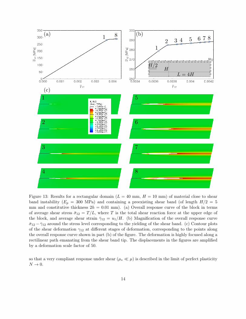
Figure 13: Results for a rectangular domain (L = 40 mm, H = 10 mm) of material close to shearband instability (Ep = 300 MPa) and containing a preexisting shear band (of length H/2 = 5mm and constitutive thickness 2h = 0.01 mm). (a) Overall response curve of the block in termsof average shear stress σ12 = T/L, where T is the total shear reaction force at the upper edge ofthe block, and average shear strain γ12 = u1/H. (b) Magnification of the overall response curveσ12− γ12 around the stress level corresponding to the yielding of the shear band. (c) Contour plotsof the shear deformation γ12 at different stages of deformation, corresponding to the points alongthe overall response curve shown in part (b) of the figure. The deformation is highly focused along arectilinear path emanating from the shear band tip. The displacements in the figures are amplifiedby a deformation scale factor of 50.

so that a very compliant response under shear (µ∗ � µ) is described in the limit of perfect plasticityN → 0.

14

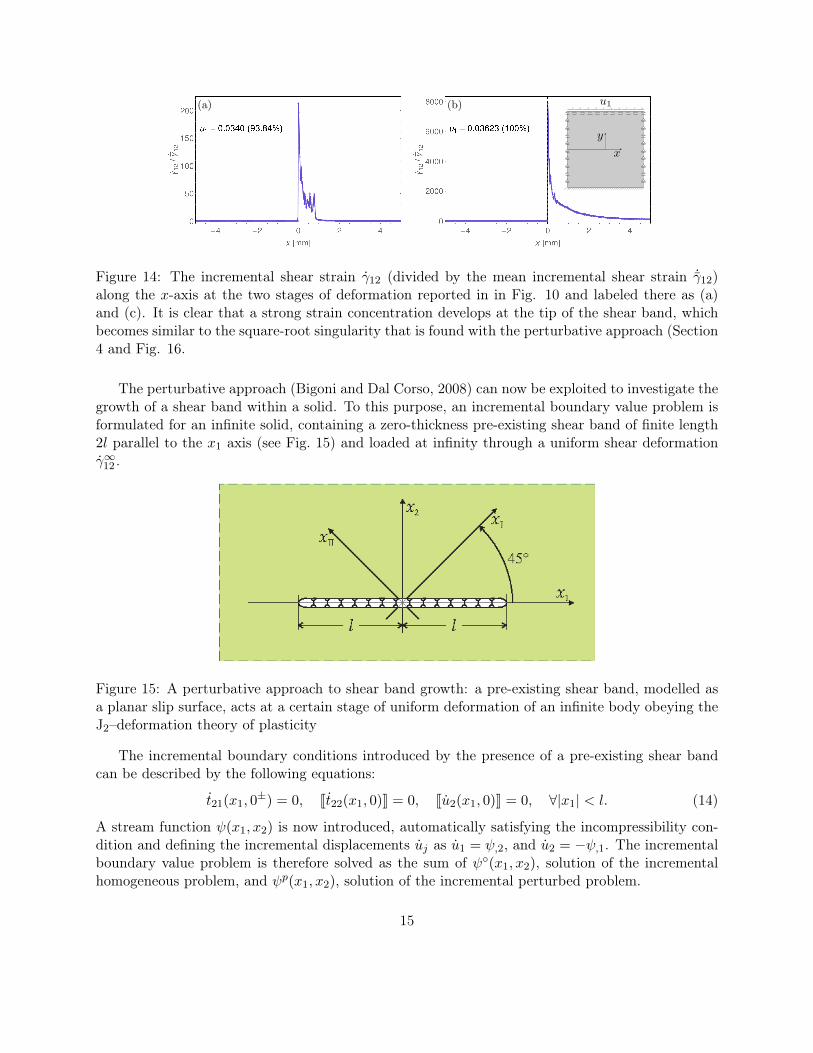
Figure 14: The incremental shear strain γ12 (divided by the mean incremental shear strain ˙γ12)along the x-axis at the two stages of deformation reported in in Fig. 10 and labeled there as (a)and (c). It is clear that a strong strain concentration develops at the tip of the shear band, whichbecomes similar to the square-root singularity that is found with the perturbative approach (Section4 and Fig. 16.

The perturbative approach (Bigoni and Dal Corso, 2008) can now be exploited to investigate thegrowth of a shear band within a solid. To this purpose, an incremental boundary value problem isformulated for an infinite solid, containing a zero-thickness pre-existing shear band of finite length2l parallel to the x1 axis (see Fig. 15) and loaded at infinity through a uniform shear deformationγ∞12 .

Figure 15: A perturbative approach to shear band growth: a pre-existing shear band, modelled asa planar slip surface, acts at a certain stage of uniform deformation of an infinite body obeying theJ2–deformation theory of plasticity

The incremental boundary conditions introduced by the presence of a pre-existing shear bandcan be described by the following equations:

t21(x1, 0±) = 0, Jt22(x1, 0)K = 0, Ju2(x1, 0)K = 0, ∀|x1| < l. (14)

A stream function ψ(x1, x2) is now introduced, automatically satisfying the incompressibility con-dition and defining the incremental displacements uj as u1 = ψ,2, and u2 = −ψ,1. The incrementalboundary value problem is therefore solved as the sum of ψ◦(x1, x2), solution of the incrementalhomogeneous problem, and ψp(x1, x2), solution of the incremental perturbed problem.

15

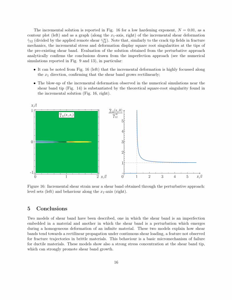
The incremental solution is reported in Fig. 16 for a low hardening exponent, N = 0.01, as acontour plot (left) and as a graph (along the x1-axis, right) of the incremental shear deformationγ12 (divided by the applied remote shear γ∞12). Note that, similarly to the crack tip fields in fracturemechanics, the incremental stress and deformation display square root singularities at the tips ofthe pre-existing shear band. Evaluation of the solution obtained from the perturbative approachanalytically confirms the conclusions drawn from the imperfection approach (see the numericalsimulations reported in Fig. 9 and 13), in particular:

• It can be noted from Fig. 16 (left) that the incremental deformation is highly focussed alongthe x1 direction, confirming that the shear band grows rectilinearly;

• The blow-up of the incremental deformation observed in the numerical simulations near theshear band tip (Fig. 14) is substantiated by the theoretical square-root singularity found inthe incremental solution (Fig. 16, right).

Figure 16: Incremental shear strain near a shear band obtained through the perturbative approach:level sets (left) and behaviour along the x1-axis (right).

5 Conclusions

Two models of shear band have been described, one in which the shear band is an imperfectionembedded in a material and another in which the shear band is a perturbation which emergesduring a homogeneous deformation of an infinite material. These two models explain how shearbands tend towards a rectilinear propagation under continuous shear loading, a feature not observedfor fracture trajectories in brittle materials. This behaviour is a basic micromechanism of failurefor ductile materials. These models show also a strong stress concentration at the shear band tip,which can strongly promote shear band growth.

16

Acknowledgments

D.B., N.B. and F.D.C. gratefully acknowledge financial support from the ERC Advanced Grant‘Instabilities and nonlocal multiscale modelling of materials’ FP7-PEOPLE-IDEAS-ERC-2013-AdG(2014-2019). A.P. thanks financial support from the FP7-PEOPLE-2013-CIG grant PCIG13-GA-2013-618375-MeMic.

References

[1] Abeyaratne, R., Triantafyllidis, N. (1981) On the Emergence of Shear Bands in Plane Strain.Int. J. Solids Struct. 17, 1113âĂŞ1134.

[2] Antipov, YA; Avila-Pozos, O; Kolaczkowski, ST., Movchan A.B. (2001) Mathematical model ofdelamination cracks on imperfect interfaces Int. J. Solids Struct. 38, 6665-6697.

[3] Argani, L., Bigoni, D., Capuani, D. and Movchan, N.V. (2014) Cones of localized shear strain inincompressible elasticity with prestress: Green’s function and integral representations Proceedingsof the Royal Society A, 470, 20140423.

[4] Argani, L., Bigoni, D. and Mishuris, G. (2013) Dislocations and inclusions in prestressed metals.Proceedings of the Royal Society A, 469, 2154 20120752.

[5] Bigoni, D. (2012) Nonlinear Solid Mechanics Bifurcation Theory and Material Instability. Cam-bridge University Press, ISBN:9781107025417.

[6] Bigoni, D. and Dal Corso, F. (2008) The unrestrainable growth of a shear band in a prestressedmaterial. Proceedings of the Royal Society A, 464, 2365-2390.

[7] Bigoni, D. and Capuani, D. (2005) Time-harmonic Green’s function and boundary integralformulation for incremental nonlinear elasticity: dynamics of wave patterns and shear bands. J.Mech. Phys. Solids 53, 1163-1187.

[8] Bigoni, D. and Capuani, D. (2002) Green’s function for incremental nonlinear elasticity: shearbands and boundary integral formulation. J. Mech. Phys. Solids 50, 471-500.

[9] Bigoni, D., Dal Corso, F. and Gei, M. (2008) The stress concentration near a rigid line inclusionin a prestressed, elastic material. Part II. Implications on shear band nucleation, growth andenergy release rate. J. Mech. Phys. Solids , 56, 839-857.

[10] Bigoni, D. Serkov, S.K., Movchan, A.B. and Valentini, M. (1998) Asymptotic models of dilutecomposites with imperfectly bonded inclusions. Int. J. Solids Struct. , 35, 3239-3258.

[11] Dal Corso, F. and Bigoni, D. (2010) Growth of slip surfaces and line inclusions along shearbands in a softening material. Int. J. Fracture , 166, 225-237.

[12] Dal Corso, F. and Bigoni, D. (2009) The interactions between shear bands and rigid lamellarinclusions in a ductile metal matrix. Proceedings of the Royal Society A, 465, 143-163.

17

[13] Dal Corso, F., Bigoni, D. and Gei, M. (2008) The stress concentration near a rigid line inclusionin a prestressed, elastic material. Part I. Full field solution and asymptotics. J. Mech. Phys. Solids, 56, 815-838.

[14] Gajo, A., Bigoni, D. and Muir Wood, D. (2004) Multiple shear band development and relatedinstabilities in granular materials. J. Mech. Phys. Solids , 52, 2683-2724.

[15] Hutchinson, J.W., Tvergaard, V. (1981) Shear band formation in plane strain. Int. J. SolidsStruct. 17, 451-470.

[16] Kirby, S.H. (1985) Rock mechanics observations pertinent to the rheology of the continentallithosphere and the localization of strain along shear zones. Tectonophysics, 119, 1-27.

[17] Mishuris, G. (2004) Imperfect transmission conditions for a thin weakly compressible interface.2D problems. Arch. Mech., 56, 103-115.

[18] Mishuris, G. and Ochsner, A. (2005) Transmission conditions for a soft elasto-plastic interphasebetween two elastic materials. Plane strain state. Arch. Mech., 57, 157-169.

[19] Mishuris, G. and Ochsner, A. (2007) 2D modelling of a thin elasto-plastic interphase betweentwo different materials: Plane strain case. Compos. Struct., 80, 361-372.

[20] Mishuris, G., Miszuris, W., Ochsner, A. and Piccolroaz, A. (2013). Transmission conditions forthin elasto-plastic pressure-dependent interphases. In: Plasticity of Pressure-Sensitive Materials.Altenbach, H., Ochsner, A., Eds., Springer-Verlag, Berlin.

[21] Piccolroaz, A., Bigoni, D. and Willis, J.R. (2006) A dynamical interpretation of flutter insta-bility in a continuous medium. J. Mech. Phys. Solids 54, 2391-2417.

[22] Puzrin, A. M. and Germanovich, L.N. (2005) The growth of shear bands in the catastrophicfailure of soils. Proc. R. Soc. A 461, 1199-1228.

[23] Rice, J.R. (1973) The initiation and growth of shear bands. In Plasticity and soil mechanics(ed. A. C. Palmer), p. 263. Cambridge, UK: Cambridge University Engineering Department.

[24] Sonato, M., Piccolroaz, A., Miszuris, W. and Mishuris, G. (2015) General transmissionconditions for thin elasto-plastic pressure-dependent interphase between dissimilar materials.arXiv:1501.02919 [cond-mat.mtrl-sci].

[25] Yang, B., Morrison, M.L., Liaw, P.K., Buchanan, R.A., Wang, G., Liu C.T. and Denda, M.(2005) Dynamic evolution of nanoscale shear bands in a bulk-metallic glass. Applied Phys. Letters86, 141904.

18