Embed Size (px)
Citation preview
JOURNAL OF GEOPHYSICAL RESEARCH, VOL. 117, F03017, doi:10.1029/2011JF002289, 2012
1
Straightforward reconstruction of 3D surfaces and topography with a camera:
Accuracy and geoscience application
James, M. R.1, Robson, S.2
1 Lancaster Environment Centre, Lancaster University, Lancaster. U.K. LA1 4YQ
2 Department of Civil, Environmental and Geomatic Engineering, UCL, Gower Street, London. U.K. WC1E 6BT
Abstract
Topographic measurements for detailed studies of processes such as erosion or mass movement are usually acquired by expensive laser scanners or rigorous photogrammetry. Here, we test and use an alternative technique based on freely available computer vision software which allows general geoscientists to easily create accurate 3D models from field photographs taken with a consumer-grade camera. The approach integrates structure-from-motion (SfM) and multi-view-stereo (MVS) algorithms and, in contrast to traditional photogrammetry techniques, it requires little expertise and few control measurements, and processing is automated. To assess the precision of the results, we compare SfM-MVS models spanning spatial scales of centimeters (a hand sample) to kilometers (the summit craters of Piton de la Fournaise volcano) with data acquired from laser scanning and formal close-range photogrammetry. The relative precision ratio achieved by SfM-MVS (measurement precision : observation distance) is limited by the straightforward camera calibration model used in the software, but generally exceeds 1:1000 (i.e. centimeter-level precision over measurement distances of 10s of meters). We apply SfM-MVS at an intermediate scale, to determine erosion rates along a ~50-m-long coastal cliff. Seven surveys carried out over a year indicate an average retreat rate of 0.70±0.05 m a-1. Sequential erosion maps (at ~0.05 m grid resolution) highlight the spatio-temporal variability in the retreat, with semivariogram analysis indicating a correlation between volume loss and length scale. Compared with a laser scanner survey of the same site, SfM-MVS produced comparable data and reduced data collection time by ~80%.
1. Introduction
Our understanding of many geomorphological processes has been significantly advanced in recent years through the use of detailed 3D spatial data. Topographic or surface models now see widespread application across the geosciences, spanning spatial scales from millimeters to multiple kilometers, and covering applications such as soil erosion and roughness measurement [e.g. Martin, 1980; Heng et al., 2010], geohazard assessments [e. g. Baldi et al., 2008; Schilling et al., 2008] and geomorphological investigations [e. g. Chandler, 1999; Lane et al., 2000; Grosse et al., 2012]. Acquiring appropriate data commonly requires expensive instrumentation and/or significant expertise, but here we demonstrate an approach that uses only digital photographs taken with a consumer camera and freely available software. With a few additional measurements for scaling and geo-referencing, the technique can deliver data suitable for many geoscience applications and offers non-experts the capability to construct 3D models from the straightforward collection of photographs at field sites. We explore the measurement precisions achievable over spatial scales of centimeters to kilometers, and then use the technique to determine spatial and temporal erosion rate variability at a coastal cliff site.
Common topographic data requirements in the geosciences extend over distances 100s of meters or more, and have traditionally been met by aerial photogrammetry, augmented nowadays by laser-based (lidar) and space-based radar and photogrammetric techniques. Airborne lidar is the current technique of choice whenever detailed topographic data over such areas are required, and usually delivers meter-scale spatial resolutions with decimetric vertical accuracy. For more restricted areas, for example, over ranges of 10s – 100s of meters, ground-based terrestrial laser scanners (TLS) are being increasingly used (e.g. for analyses of landslides [Teza et al., 2007], rockfall [Abellan et al., 2009] and coastal change [Rosser et al., 2005]). The most modern close-range scanners offer millimeter accuracies, and decreased size, weight and cost compared to their predecessors, and very-long-range instruments have proved effective at distances up to 3500 – 4000 m in glacial and volcanic environments [Schwalbe et al., 2008; James et al., 2009].
Nevertheless, camera-based approaches retain advantages over laser scanning for applications requiring detailed data from remote, rapidly changing or spatially limited areas, through their low cost nature and low bulk. Furthermore, unlike laser scanners, cameras can be easily mounted on light weight unmanned aerial platforms such as kites [Smith et al., 2009] and model helicopters [Eisenbeiss et al., 2005; Niethammer et al., 2010] to obtain near-vertical coverage. However, adoption of image-based techniques in the geosciences has been restricted by the learning curve involved and the specialist (usually commercial) software required to carry out traditional photogrammetry processing. Commonly, image collection, data processing and DEM derivation have used procedures derived directly from aerial photogrammetric approaches based on stereo-pairs [e.g. Chandler et al., 2001; Chandler et al., 2002; Bird et al., 2010; Gessesse et al., 2010]. In such cases, general practical requirements (determined by processing software) are relatively restrictive; images should be taken nearly parallel and with ~60% overlap, and control points with known coordinates must be observable in the images. With expertise, some of these restrictions can be relaxed to provide more flexible image capture [Chandler, 1999], but deployment and accurate measurement of control points may be difficult and time consuming. Stereo-based approaches are also sensitive to errors in camera calibration and can lack redundancy because only two images are used simultaneously for DEM generation.

JOURNAL OF GEOPHYSICAL RESEARCH, VOL. 117, F03017, doi:10.1029/2011JF002289, 2012
2
Recently, the acquisition of topographic data from consumer-grade cameras (both from the ground and from the air) has been facilitated by the application of close-range and oblique photogrammetry techniques (e.g. for lava flows and domes [James et al., 2006; James et al., 2007; Ryan et al., 2010; Diefenbach et al., 2012a; Diefenbach et al., 2012b]), but the requirements of practical expertise and obtaining control points remain.
The technique described here is based on freely available software that combines the computer vision approaches of ‘structure-from-motion’ (SfM [Ullman, 1979]) and ‘multi-view stereo’ (MVS [Seitz et al., 2006]). SfM algorithms were originally developed for the automatic generation of 3D models from unordered image collections [Brown and Lowe, 2005], for example, color reconstructions of iconic buildings using only images downloaded from the internet [e.g. Snavely et al., 2006; 2007]. The SfM approach requires multiple images of a scene taken from different positions and simultaneously calculates camera parameters and orientations, and a sparse 3D point cloud representing the most prominent features in the images. The Photosynth web site (photosynth.net) provides a very accessible interface to an online SfM service, and can be used to obtain sparse point clouds. Consequently, use of SfM on its own has been previously explored for micro-DEM generation of bare rock surfaces [Dowling et al., 2009], investigation of vegetation structure [Dandois and Ellis, 2010] and geology visualization [Stimpson et al., 2010]. However, without further processing, SfM results are insufficiently detailed and too noisy for high quality surface reconstructions [Rosnell and Honkavaara, 2012].
Recently, refined 3D reconstruction software has significantly increased the detail and quality of the resulting models by linking SfM output with MVS image matching algorithms. The MVS process efficiently filters out noisy data and typically increases the number of reconstructed points by two or three orders of magnitude. The resulting point clouds are of sufficient quality to generate DEMs, but do not have any scale or geospatial information. Consequently, control measurements are needed to geo-reference the models. Nevertheless, such measurements are not used within the model development process and their requirements are thus significantly less onerous than for formal photogrammetric techniques. The use of such a combined SfM-MVS approach is already being explored within disciplines such as archaeology [Verhoeven, 2011] and palaeontology [Falkingham, 2012], and useful results have been demonstrated with images from UAVs and light aircraft for mudslide [Niethammer et al., 2010; Niethammer et al., 2011] and glacial [Welty et al., 2010] analyses, and from ground-based images for assessing gully erosion [Castillo et al., 2012] and lava flow processes [James et al., 2011].
As a specific demonstration of the advantages of SfM-MVS, we illustrate its use for assessing the retreat of a coastal cliff. Cliff erosion processes have been studied recently using airborne and ground-based lidar, and photogrammetry [Young et al., 2009; Lim et al., 2010; Young et al., 2011], where the high density of the measurements produced enables sophisticated geostatistical [Harley et al., 2011] and geotechnical [Quinn et al., 2010] analyses. By enabling automated reconstructions to be carried out with minimal control measurements, SfM-MVS offers the potential for significantly reducing the expertise and time required for generating such DEMs or surface models. However, few metrics are provided to quantify the quality of the results and previous work has not assessed the general error processes involved in any detail. Consequently, prior to using SfM-MVS to assess cliff retreat, we use case studies over a range of scales and scenarios (a volcanic bomb hand sample ~10 cm across, and a ~1×1.5 km area covering the summit craters of Piton de la Fournaise volcano ) to identify and quantify the inherent limitations of the SfM-MVS technique for geoscience studies. We provide a software tool for scaling and geo-referencing the results and compare the accuracy using data from benchmark techniques (laser scanning and formal close-range photogrammetry). We then assess and validate SfM-MVS performance at a ~50-m-long coastal cliff site and use seven surveys collected over a year to determine erosion rates and characteristics.
2. Methodology and software
Throughout this work we use digital SLR cameras and fixed focal length lenses because of their high image quality. Relatively wide angle lenses (e.g. equivalent to 35 mm on a traditional SLR camera) are best for 3D geometry reconstruction. Significantly longer lenses, for example those with focal lengths of order three or more times the diagonal distance across the sensor, are increasing difficult to produce accurate results from (for the APS format sensors typical in consumer digital SLRs, this equates to focal lengths >90 mm). Fisheye lenses should also be avoided because they can only be represented accurately by specialist camera models. A camera model (or ‘camera calibration model’) describes the internal optical geometry that determines how the image is formed in the camera. Usually, camera models contain several parameters to describe lens distortion, but fisheye lenses involve more complex distortion patterns that are poorly represented by standard models. Compact cameras and camera phones could also be used, but they may not achieve the precisions given here [e.g. Goesele et al., 2007].
One of the main advantages of SfM-MVS over traditional photogrammetry is that a wide range of images can be automatically processed. Nevertheless, consideration of a few principles during image collection can help minimize the acquisition of photographs that may be rejected during analysis. Fundamentally, SfM-MVS reconstruction works by matching image texture in different photographs, and determines 3D geometry under the assumption that the scene is static. Consequently, areas showing little texture in the images (e.g. featureless areas such as a flat sandy beach, blanket snow cover or areas obscured by strong shadow) will not be reconstructed. To avoid strong shadows, illumination conditions are ideally diffuse, such as during bright but overcast days. Factors that cause the surface to vary its appearance from different directions (such as using a camera flash or imaging reflections or glints from wet surfaces) should be minimized. Depending on the scale of the imagery, vegetation can fall in this category, for example, results will be poor or sparse in areas where multiple overlapping stems or moving leaves can be resolved [Castillo et al., 2012]. Although SfM-MVS algorithms are tolerant to images taken at different scales, extreme variations caused by large zooms or by photos taken at significantly different distances to the surface (which effectively changes the image texture representing the surface) can cause images to be rejected.
For 3D reconstruction, SfM-MVS analysis requires images of the area of interest to be acquired from different positions and the algorithms are designed to work with convergent imagery, i.e. camera orientations are not parallel, but rather converge on the scene.

JOURNAL OF GEOPHYSICAL RESEARCH, VOL. 117, F03017, doi:10.1029/2011JF002289, 2012
3
With digital photographs easy to acquire and the processing automatic, the procedure adopted is to collect more images than necessary to reduce the chance of accidentally omitting areas. Consequently, we aim for relatively short distances between photo positions (for example, 2-3 m when imaging over ~20 m) and photos at angular intervals of 10-20°, over as wide a range of angles as possible. Good results can be achieved from image sets of 10s to 100s of images (see the case study figures for examples of appropriate camera positions). The actual number required will vary with the size and complexity of the project but any specific region to be reconstructed must be observable in a minimum of three images.
For scaling and geo-referencing the resulting point clouds, control points should be located towards the edge or outside of the area of interest, so that coordinate transformations are not being extrapolated outside the volume encompassed by the control. Although a minimum of three control points are needed to enable geo-referencing, more control provides a more robust solution which is less sensitive to error on any one point. In the field, control point coordinates can be acquired using GPS or a total station survey at most sites. However, if scale alone is required, then only distances between features are needed, which can be obtained, for example, with a tape measure. Control distances measured across the full area to be reconstructed will provide a more accurate scaling than shorter measurements.
2.1. SfM-MVS software
A number of internet services and an increasing number of commercial products now incorporate SfM and MVS approaches to reconstructions from photographs. Here we use a freeware implementation (http://blog.neonascent.net/archives/bundler-photogrammetry-package/ by J. Harle) that combines the commonly used SfM application ‘Bundler’ [Snavely et al., 2006; Snavely et al., 2007; Snavely et al., 2008], with the MVS dense matcher ‘PMVS2’(Patch-based Multi-View Stereo, [Furukawa and Ponce, 2007; 2010]). The software requires a 64-bit computer with an Nvidia graphics card, running a Microsoft Windows operating system. RAM requirements are driven by the MVS step and vary with the size and number of the images used, and the density of the reconstruction. All the reconstructions in this paper were initially carried out on a Windows 7 laptop with 6 Gb RAM but, for speed, repeat analyses were carried out on a 12-Gb-RAM desktop machine. To use the software, the image files are copied into a folder and two run-scripts are executed to perform the automatic reconstruction.
2.1.1. Structure-from-motion
To start the SfM reconstruction process, all images are processed by an automatic feature-detection-and-description algorithm called SIFT (Scale Invariant Feature Transform [Lowe, 2004]). An image ‘feature’ represents a distinctive area of image texture that it is likely to be identifiable in other images. The most prominent features are then matched in different images within the image set. For 3D geometry reconstruction, Bundler uses the resulting network of matched features and, starting with one image pair and incrementally adding images, determines the camera model parameters (a focal length and two radial distortion parameters per image) and the camera orientations (position and direction). Simultaneously, 3D coordinates for the feature points are computed. The resulting sparse point-cloud (typically only a few tens of thousands of points) thus represents the 3D coordinates of the most prominent features within the image set.
2.1.2. Multi-view stereo
The subsequent dense MVS matching process is then carried out by PMVS2 to provide a detailed 3D model. PMVS2 generates large numbers of points by working over a grid of pixels in an image, effectively searching for the best matches for each grid cell [Furukawa and Ponce, 2007]. The size of the grid steps can be varied to control the number of points produced and the time taken; all reconstructions here were carried out at intermediate densities, effectively down-sampling the images by a factor of four or eight. The default values provided by the software are recommended for most projects.
PMVS2 is memory intensive because all the images to be matched are processed simultaneously; memory requirements increase with the size and number of images, and with greater requested reconstruction densities. RAM availability provides practical limits on how many images PMVS2 can match simultaneously. To permit matching with large image collections, a pre-processing step, CMVS (Clustering Views for Multi-View Stereo [Furukawa et al., 2010]) is integrated into the software. The CMVS process uses the camera orientations and surface points output by Bundler to automatically select and group images, based on scene visibility, into optimized clusters for sequential PMVS2 processing. The final point clouds used here are the results of multiple dense matches with PMVS2 only, and the original sparse point clouds from the SfM process, which are prone to significantly greater noise, are discarded.
2.2. Scale and geo-referencing
Scaling and geo-referencing of SfM-MVS models can be carried out by identifying known features in the point cloud [e.g. Dowling et al., 2009; Dandois and Ellis, 2010; James et al., 2011]. However, it can be difficult to accurately identify small features in point cloud data, and the precision of any coordinates determined is limited by the local reconstruction density. We developed a Matlab® software tool, sfm_georef, to allow feature coordinates to be determined directly from the images. Using the camera models and orientations defined by the SfM output, observed features in the images can be used to calculate their 3D point coordinates in the SfM coordinate system. These coordinates can then be used to derive the transformation required (usually a scaling, rotation and translation) to convert the SfM coordinate system to that of the control data. One of the principal drawbacks for quantitative SfM-MVS use with Bundler and PMVS2 is that it is difficult for a typical user to assess the reconstruction quality from the error metrics provided. For scaling and geo-referencing with sfm_georef, we attempt to address this by providing the image intersection and control point residual results that are familiar in traditional aerial photogrammetry software.

JOURNAL OF GEOPHYSICAL RESEARCH, VOL. 117, F03017, doi:10.1029/2011JF002289, 2012
4
For cases in which models require only an appropriate scale (e.g. hand samples, for which absolute geo-referencing is not relevant), projects can be scaled by identifying one or more known distances. If more than one distance is used, an optimum scaling factor that minimizes the least-squares error of the distance measurements is determined. If geo-referencing is required, three or more points with known coordinates must be identified. If more than three points are identified, then a least-squares best fit to the reference points is determined. Sfm_georef allows determination of the transform and subsequent conversion of PMVS2 output files.
2.3. Sources of reconstruction error
In SfM-MVS computer vision research, the focus is on producing realistic and appealing 3D reconstructions from as wide a range of unconstrained imagery as possible, and results are not subject to the rigorous investigations of metric precision that are standard within the photogrammetric community. Consequently, quantitative applications of the approach need to be validated. Error metrics for the scaling and geo-referencing step are provided by sfm_georef, but internally the accuracy of SfM-MVS reconstructions may be limited by three main factors:
(1) the SIFT algorithm used in the SfM step has proved powerful for matching disparate imagery but can produce relatively poor feature-position precision [Remondino, 2006; Barazzetti et al., 2010b]. This has the potential to degrade the accuracy of the recovered camera models and their orientations, and hence to influence overall reconstruction accuracies.
(2) The straightforward camera calibration model used by Bundler should reproduce most of the distortion in many consumer cameras, but the calibration model is not as refined as those used in established photogrammetric models [e.g. Luhmann et al., 2006]). Issues arising from the limited camera model are likely to be most evident in areas toward the image edges, where distortion effects are greatest.
(3) For many scientific applications, images are typically acquired using one camera with a fixed lens, which requires only one camera model to be optimized. However, Bundler does not offer this specific constraint under general use. Instead, each image is considered to have been obtained by a camera that is independent of all others, and therefore multiple camera models must be computed. Although this approach is understandable given the original aims of SfM research, it could be an additional source of error if only one camera (with fixed internal geometry) has been used for all images in a reconstruction. Independent camera models can be a particular issue in linear sequences of images, where the incremental image assimilation approach used by Bundler can lead to drift of the estimated camera parameters along the image sequence, resulting in distorted reconstructions [Barazzetti et al., 2010a].
These factors result in reconstruction accuracies for SfM-MVS approaches that are generally much less than those delivered by standard photogrammetric techniques [Goesele et al., 2007]. We use the case studies below to not only characterize the overall precision of the reconstructions, but also to determine how these internal limitations influence the results. We focus our analysis on comparisons of the 3D surface results. For technical data on the recovered camera parameters we refer the interested reader to the auxiliary material. [Auxiliary materials are available in the HTML. doi:10.1029/2011JF002289]
3. Hand-sample-scale case study: volcanic bomb To analyze SfM-MVS use at decimeter scales, a volcanic bread-crust bomb sample from Soufriere Hills volcano, Montserrat
(Figure 1) was reconstructed. The sample was selected because its complex ‘bread-crust’ surface provides a good test of the detail achievable in a laboratory-scale reconstruction. A successful model allows quantification of bread-crust morphology as well as overall sample shape.
3.1. Data acquisition and processing
Two hundred and ten images (4272 × 2848 pixels) were taken with an EOS 450D camera and 50 mm fixed focal length lens, in a bright, naturally lit, indoor area. For convenience, the sample was placed on a turntable and rotated. At the sample, the lighting was diffuse, which ensured that textural differences in the images were not due to sharp shadows that varied with rotation. At imaging distances of ~0.7 m, the depth of field could not fully encompass the sample, so the lens was set to autofocus to maintain optimal image quality throughout the image set. Most images were taken with the camera on a tripod (at various heights) but a few near-vertical images were taken by hand. In order to fully cover the sample, 124 images were taken with the sample one way up, then the sample was inverted on the turntable and another 86 images acquired. For this approach to be successful, the sample had to provide the dominant texture in all the images so that the SfM algorithm would consider the sample to be stationary (and the camera moving) and thus register all images within a common sample-centric coordinate system. Consequently, the turntable had a plain surface and was placed against a black background (Figure 1a). Black dots (Figure 1a, lower inset) were printed on the turntable surface to enable scale distances to be measured. Although scale could be determined from one distance measurement alone, multiple different measurements allowed scale errors to be reduced. Following image capture, 6 distances (between 99 and 215 mm long) were measured between 4 dot markers using a steel rule (to an estimated precision of ~500 µm each), and a best-fit scale calculated.
The full 3D shape of the sample was also measured with a state-of-the-art laboratory-based Arius3D laser scanning system, at an effective point spacing of 100 µm, and positional accuracy of 25 µm. The scaled SfM-MVS model was compared with the benchmark scanner model by mutually aligning them using an iterative closest-point technique for point cloud alignment in Arius3D PointStream software.
3.2. Reconstruction results and comparisons
All 210 images acquired were successfully processed by the SfM algorithm (Figure 1b) and scaling produced an RMS error of 110 μm over the scale distances. Of these 210 images, the CMVS process automatically selected 92 (grouped into 5 clusters) for dense

JOURNAL OF GEOPHYSICAL RESEARCH, VOL. 117, F03017, doi:10.1029/2011JF002289, 2012
5
matching and production of the final model (Figure 1c). Orthogonal cross sections through the SfM-MVS and scanner models (Figure 1c, d) show that the majority of the SfM-MVS data provides a good fit to the scanner data; the largest differences represent areas of steep faces where small lateral differences, or missing data, produce large apparent offsets (Figure 1d, upper inset). Despite this, the differences between radial distances for the model sections (averaged over 1° increments, Figure 1d) have means of 69 and 110 μm for the x- and y-sections respectively, with associated RMS values of 311 and 298 μm.
4. Hill-scale case study: Summit craters of Piton de la Fournaise To consider a contrasting scale and scenario from those of the hand-sample, we use an image sequence taken of the kilometer-wide
summit region of Piton de la Fournaise volcano in 2003 (Figure 2a). In order to test a reconstruction algorithm being developed at that time [Cecchi et al., 2002; Cecchi et al., 2003], 45 ground control points (GCPs) constructed of white sheets were deployed (those nearest the summit region are shown in Figure 2d and insets in Figure 2a) and their positions recorded by dGPS to an estimated precision of 0.1 m [B. Van Wyk de Vries, 2011, pers. comm.].
4.1. Data acquisition and processing
One hundred and thirty three images (3072×2048 pixels) were acquired from a micro-light aircraft hired for tourist over-flights on two different days, using a Canon EOS D60 camera with fixed 20 mm focal length lens. In contrast to the sample-scale study the lens focus ring was fixed for stability, so that a single camera model should be appropriate for all images. This constraint allowed further analyses to be carried out to assess the limitations of Bundler’s camera model and to determine the effects of using independent models for each image. Thus, two additional reconstructions were carried out: first, a single Bundler-style camera model (which has only two radial distortion coefficients) was used for all images; second, a single, but more sophisticated camera model was used, in which the parameter set was extended to include the additional distortion terms often used in conventional photogrammetry (principal point offsets, a third radial term, two tangential terms, orthogonality and affinity).
The additional models were calculated by importing the SfM results into the close-range photogrammetry software VMS (Vision Measurement Software, http://www.geomsoft.com, Robson & Shortis) for reprocessing. In VMS, after selecting the appropriate camera model, a bundle adjustment was carried out, which simultaneously optimizes the camera model and camera orientations, as well as the 3D point coordinates. The two sets of reprocessed SfM results were then returned to PMVS2 for dense matching. All three SfM-based models were independently geo-referenced using the GCP data.
Owing to volcanic activity there are no accurate pre-existing topographic data of the summit area. However, the large numbers of GCPs allowed a reference surface to be derived from close-range photogrammetry using VMS and the dense stereo matcher ‘Gotcha’ (Gruen-Otto-Chau) [Gruen, 1985; Day and Muller, 1989; Otto and Chau, 1989]. As a stereo algorithm, Gotcha can only match two images at a time, and does so by attempting to find points in a second image that correspond to a defined grid of pixel locations in a primary image. To enable multi-image matching, suitable images were manually grouped into 14 image sets, with each set comprising one primary image and a suite of others. Gotcha was run repeatedly within each image set to match all images to the primary image and the results were then merged to produce a multi-view match for each group.
Initial camera orientations were estimated in VMS by identifying the control points in all the images. The orientations were then refined by importing a subset (~7000) of the matches and carrying out a bundle adjustment, before a dense 3D point cloud was derived from the full set of merged matches. For direct comparisons, all point clouds (photogrammetry and SfM-MVS-derived) were interpolated into 2-m interval DEMs, using Surfer® software.
4.2. Reconstruction results and comparisons
The SfM process successfully incorporated all images (Figure 2b), with MVS matching resulting in a dense point cloud of ~2.2×10⁶ points in the summit region (Figure 2c, Table 1). Using all the control points to scale and geo-referencing the model for DEM generation (Figure 2d) resulted in an RMS misfit to the control of 0.99 m.
In comparison with the point cloud produced by the close-range photogrammetry approach, the SfM-MVS results were denser (more points per m2), but less evenly distributed (Figure 3a, b), particularly on the summit flanks. This is probably due to areas of low image texture in which the PMVS2 matcher did not reconstruct surface points, but where the Gotcha matcher (which implements a different style of algorithm) could successfully bridge from surrounding areas of greater texture. The overall density of both point clouds could have been increased by using different match parameters, but this was not necessary in order to get ~1 measurement per m2 over most of the summit area. A cross section through all point clouds (Figure 3c) illustrates the differences prior to DEM creation. The enlarged excerpts demonstrate that there is a systematic difference between reconstructions at the west end of the section, but no systematic difference is seen in the central crater area.
The differences between the reconstructions are more clearly visible when comparing the derived DEMs (Figure 4). The vertical differences between the VMS-Gotcha and the SfM-MVS DEMs show general agreement at the meter-level within the craters (an overall RMS difference of 1.0 m for the entire area shown in Figure 4a), but areas of systematic differences of around 2 m to the west and north east. Within the two boxed regions (Figure 4a), the mean differences were 0.15 and 0.10 m for the west and east regions respectively, with associated RMS values of 0.41 and 0.56 m. Reprocessing the Bundler output for just one camera model results in reducing the error in the west (Figure 4b), but increases error in the region of the north wall of the main crater. Increasing the number of camera parameters reduces overall error; RMS error on the control decreases to 0.26 m, and RMS difference across the entire DEM is 0.87 m. However, these improvements are dominantly to the margins of the reconstruction and the mean and RMS difference values for the boxed areas (Figure 4a) remain between 0.1 – 0.2 m and 0.4 – 0.6 m respectively.

JOURNAL OF GEOPHYSICAL RESEARCH, VOL. 117, F03017, doi:10.1029/2011JF002289, 2012
6
The large number of control points used in the geo-referencing allows the internal consistency of the SfM-MVS model to be assessed. However, deploying this many GCPs is time consuming and may be unrealistic in many situations. To assess the sensitivity of the geo-referencing to a more restricted deployment of control points, the effect of deriving the coordinate transformation from only a subset of the GCPs can be considered. For example, selecting only five central GCPs (given by the circled control points in Figure 2d) gives an RMS error to control of 0.11 m and an RMS error to all the unused GCPs of 1.38 m. If five GCPs are selected away from the center, such as those outlined by squares in Figure 2d, then geo-referencing error is extrapolated across the reconstruction (up to distances of ~1600 m) and RMS error to the unused GCPs increases to 2.09 m. In both of these cases, the calculated scale factor is within ±0.1 % of that determined when all GCPs are used for geo-referencing.
5. Coastal erosion at outcrop-scale: Coastal cliff section
We applied the SfM-MVS method to study erosion at an outcrop scale, over a ~3-m-high by 50-m-long section of coastal cliff located at Sunderland Point, Morecambe Bay, U.K. (Figure 5). The cliff is composed of unconsolidated, poorly sorted glacial tills and is undergoing retreat through intermittent slumping and collapse. Seven SfM-MVS surveys were carried out between 12 February 2011 and 3 March 2012 to estimate erosion rate. At the time of the first survey the cliff had several undercut regions (Figure 6) and a volume of previously slumped material at the foot of the cliff (Figure 5b, c). Although the cliff face provides reasonable image texture for feature extraction and matching (Figure 5b, inset), the long and thin geometry of the site is not optimal for SfM-MVS reconstruction because images can be taken in a linear sequence only, rather than in 360° loops as for the previous examples (Figs. 1b, 2b). Consequently, before using the SfM-MVS models to determine erosion rates, we validate the first survey (12 February 2011) using TLS data collected at the same time. In particular, we analyzed the SfM-MVS data for any model distortion that may reflect drift of estimated camera parameters along the photograph sequence.
5.1. Data acquisition and processing
Data for all SfM-MVS surveys were collected in a similar manner, using a Canon EOS 450D camera with a 28 mm fixed focal length lens. Setting the aperture to f/11 provided a depth of field of between ~2 m and infinity, allowing the internal camera geometry to be fixed throughout all images by selecting manual focus and taping the focus ring to prevent accidental movement. In the first survey, a total of 133 images (Figs. 5b, 6a) were acquired. For comparison with the TLS data, two additional models were also produced (as for the hill-slope scale example) using VMS to reprocess SfM results prior to the dense matching. One reconstruction restricted the camera models to only one Bundler-style model and the second used one, extended camera model.
The comparison data were collected with a Riegl Z210ii terrestrial laser scanner. The Z210ii has a quoted range accuracy of 15 mm (under Riegl test conditions), with a beam divergence of 2.7 mrad (0.15°). The instrument was used at minimum distances of 20-30 m from the cliff, and at angular increments of 0.018°, representing spot diameters and measurement intervals of 5-8 cm and 6-9 mm respectively. Data from three scanner positions (to cover the full cliff) were geo-referenced using differential GPS control points and merged into a single point cloud using an iterative closest point algorithm within the Riegl software (RiScanPro v1.5.1b11).
In order to scale and geo-reference the SfM-MVS reconstructions, eight points were identified that were expected to be consistent through all surveys (the tops of fence and groyne posts on the cliff top and foreshore respectively, Figs. 5b, 6a). Using eight control points provided redundancy and also enabled any identification mistakes in the geo-referencing (that showed as large residuals) to be isolated and corrected. Not all control points were easily accessible for GPS measurement so, for consistency, all point coordinates were determined from the geo-referenced TLS point cloud. Using sfm_georef, the same points were identified in the image sets, their SfM-space coordinates determined and the transform to the TLS coordinate system calculated and applied. Each SfM-MVS survey was independently geo-referenced using the same eight control points from the TLS data.
5.2. Reconstruction results and comparisons
For the first SfM-MVS model acquired (Figure 5c), geo-referencing gave an RMS error of 37 mm on the control points. With the control point locations encompassing the full length of the cliff (Figure 6a), the reconstruction scale is relatively well determined. Consequently, if the control used for geo-referencing is restricted to only the three most dispersed points, the scale changes by only 0.01%, but the RMS error on the unused points increases to 50 mm. This wide control distribution can be compared with results from a more restricted distribution. If the three control points used are at the west end only (two on the shore and one on the cliff), scale changes by 0.17% and the RMS error on the unused points increases to 181 mm. This magnitude in difference in scale and RMS highlights the sensitivity of the geo-referencing when control is focused in only one region.
Although SfM-MVS reconstructions compare well with the TLS model when all eight control points are used, differences in cross-sections of up to ~0.1 m are observed (section A-A', Figure 6b). To examine the extent to which this could be geo-referencing error, the alignment of the SfM-MVS model to the TLS model was refined by using an iterative closest point adjustment in PointStream software. Following this adjustment (which varies the model orientation only, the scale remains unchanged), the results for the SfM-MVS model and both VMS-reprocessed SfM-MVS models overlay the TLS model closely (Figure 6c).
To enable a fuller comparison of data across the cliff face, the point clouds have been converted to raster-based surfaces by transforming them into a vertically-oriented cylindrical coordinate system. Radial values are then interpolated over an azimuth-z grid (with angular limits indicated in Figure 6a) to represent the cliff face on a curved, vertical grid. The grid intervals used were 0.05 m vertically and 0.085° in azimuth which, at the average radial distance for the cliff of ~32 m, represents a mean horizontal distance of ~0.05 m over the cliff face. Grid values with fewer than 5 data points in the interval were discarded. Comparison of the TLS and SfM-MVS cylindrically gridded models shows they differ by less than ~20 mm over much of the cliff face (Figure 7). No significant

JOURNAL OF GEOPHYSICAL RESEARCH, VOL. 117, F03017, doi:10.1029/2011JF002289, 2012
7
systematic errors (indicative of sequential drift of the recovered camera parameters) are observable in the standard SfM-MVS reconstruction (Figure 7a). Furthermore, the reprocessing procedures showed no significant improvement over the basic SfM-MVS workflow (Figure 7b-d).
For the entire region shown in Figure 7a, the differences between the interpolated SfM-MVS and TLS results have an RMS error value of 70 mm. For the single camera and single, extended camera models, the RMS error is 74 and 67 mm respectively. However, the error magnitude is strongly influenced by spatial differences in data collected at the top and base of the section, and at the crests of slumps where vegetation and oblique angles complicate the comparison. This is illustrated by the three ~1 m2 boxed areas in the middle of the cliff (Figure 7a), which have RMS differences of 13, 12 and 95 mm for the left, middle and right area respectively. The left and middle areas cover bare, near vertical cliff face (Figure 5b, c) whereas the right area (Figure 5b, c, 8) covers the top of a slump. Where the point clouds overlap, there is little observable difference between the TLS and SfM-MVS data (Figure 8c). However, during the gridding procedure the differences in data density and spatial coverage result in sizable grid differences near the edges of partly occluded areas (Figure 8b).
5.3. Erosion rates
All SfM-MVS surveys of the cliff provided similar quality data, with RMS error on the control varying between 28 and 55 mm. Cliff evolution over the study period included multiple collapse events and erosion of the cliff foot (Figure 9). For an estimate of the error magnitudes involved when comparing surveys, in line with the RMS errors on the control points, we consider a potential relative offset of 50 mm between the surfaces. Over the area of the full cliff face, this represents 7.2 m3. Total volume loss (Figure 9a) was thus 100.6±7.2 m3, equating to 2.12±0.15 m3a-1 per meter of cliff or a mean retreat rate of 0.70±0.05 m a-1.
Strong seasonal variability is shown with June and July experiencing negligible change. The most significant period of loss (18 October – 30 November 2011) included the passage of a European windstorm during which strong onshore winds coincided with a high tide (25 November, at 12:00, with a tidal height of 10.19 m measured at Heysham Port, ~6 km to the north, and winds from WSW to NW at 25-28 knots recorded at Hazelrigg weather station, ~7 km to the east). During such events, the cliff is subject to direct wave attack.
The large number of erosion measurements effectively made during each interval (i.e. ~60,000 cells in each azimuth-elevation grid, Figure 9) supports rigorous geostatstical analysis of spatial variability of erosion. Here, we use semivariogram analysis [Schuenemeyer and Drew, 2011] that characterizes the degree to which a measurement at one location is related to measurements at other points a specific distance (or ‘lag’) apart. At a lag of zero, the semivariance should be zero; semivariance increases with increasing lag toward the overall variance value for the data (Figure 10a). The ‘range’ or correlation length characterizes the lag over which points are similarly influenced; at long distances the spatial dependence between data points is lost. For the cliff erosion data, calculated correlation lengths for each period show a relationship with the associated measured volume loss in which larger volumetric losses are linked with longer correlation lengths (Figure 10).
6. Discussion
The case studies demonstrate that the SfM-MVS approach can produce surface or topographic data over scales and scenarios relevant to a broad range of geoscience applications. The characteristics summarized in Table 1 highlight the rapid and affordable nature of SfM-MVS data collection compared to laser-based approaches. Although the computational part of the reconstruction process can be time consuming, the automation of the approach means that the process runs with minimal human intervention. In part, reconstruction durations result from the capability of being able to use unordered image collections; each image is initially tested for matches against all others in the project. Consequently, appropriately reducing the number of images and refining match parameters can significantly decrease reconstruction time, so determining guidelines for such optimization, particularly in terms of strategies for more efficient image collection, is a useful area for future work. To describe reconstruction qualities we use a relative precision ratio, which compares the precision of the 3D data obtained to the average viewing distance used (i.e. the mean camera-to-surface distance). This convenient expression can be used in planning SfM-MVS projects to ensure that the required precisions are achieved. General estimates for expected error magnitudes can be considered in two broad classes: (1) the quality of the overall project geometry, scaling and geo-referencing, in which any large-scale distortions show as poor fit to control, or as long-wavelength systematic error trends in surface comparisons; and (2) the quality of surface reconstruction on the local scale, where poor quality results in noisy surfaces.
6.1. Scale, geo-referencing and project geometry (SfM) error
The camera models and orientations that define the overall imaging geometry are calculated by Bundler in the SfM step. If sufficient control data are available, the quality of the reconstructed project geometry is indicated by the residual error about the control. Where geometry has been accurately determined, the error magnitudes determined during geo-referencing should approach those of the control point measurements. If control availability is more restricted, and particularly, where it is located in a limited region, then geo-referencing errors can increase across a reconstruction.
For the geological hand sample, only scale was determined. Six control measurement distances, with an estimated measurement precision of 0.5 mm over an average control distance of 165 mm, gave a representative distance error of ±200 μm, or a scale error of ~0.1 %. In the modeled surface reconstruction, the RMS error to the control distances was 110 μm. Therefore, the reconstruction of the control lengths was better than or equal to the error magnitude of the control measurements. For the sample itself, over mean x- and y- cross-sectional radii of 56 and 50 mm respectively, corresponding differences between the SfM-MVS reconstruction and the laser
JOURNAL OF GEOPHYSICAL RESEARCH, VOL. 117, F03017, doi:10.1029/2011JF002289, 2012
8
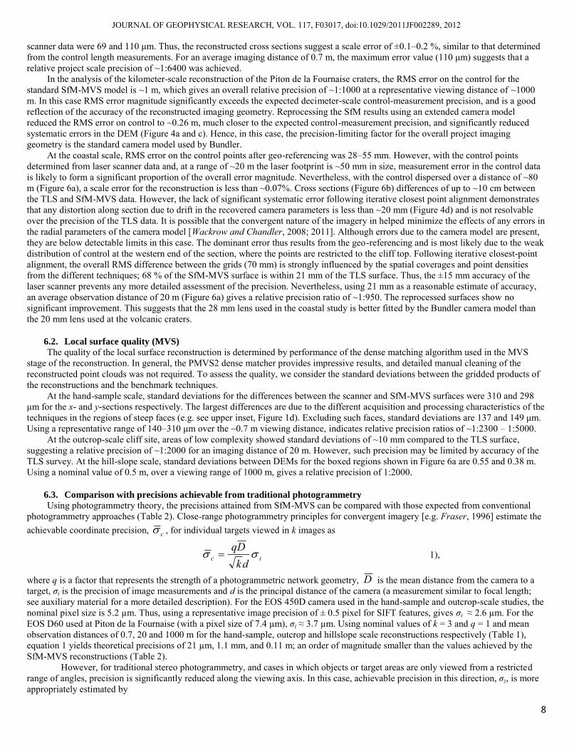
scanner data were 69 and 110 μm. Thus, the reconstructed cross sections suggest a scale error of ±0.1–0.2 %, similar to that determined from the control length measurements. For an average imaging distance of 0.7 m, the maximum error value (110 μm) suggests that a relative project scale precision of ~1:6400 was achieved.
In the analysis of the kilometer-scale reconstruction of the Piton de la Fournaise craters, the RMS error on the control for the standard SfM-MVS model is ~1 m, which gives an overall relative precision of ~1:1000 at a representative viewing distance of ~1000 m. In this case RMS error magnitude significantly exceeds the expected decimeter-scale control-measurement precision, and is a good reflection of the accuracy of the reconstructed imaging geometry. Reprocessing the SfM results using an extended camera model reduced the RMS error on control to ~0.26 m, much closer to the expected control-measurement precision, and significantly reduced systematic errors in the DEM (Figure 4a and c). Hence, in this case, the precision-limiting factor for the overall project imaging geometry is the standard camera model used by Bundler.
At the coastal scale, RMS error on the control points after geo-referencing was 28–55 mm. However, with the control points determined from laser scanner data and, at a range of ~20 m the laser footprint is ~50 mm in size, measurement error in the control data is likely to form a significant proportion of the overall error magnitude. Nevertheless, with the control dispersed over a distance of ~80 m (Figure 6a), a scale error for the reconstruction is less than ~0.07%. Cross sections (Figure 6b) differences of up to ~10 cm between the TLS and SfM-MVS data. However, the lack of significant systematic error following iterative closest point alignment demonstrates that any distortion along section due to drift in the recovered camera parameters is less than ~20 mm (Figure 4d) and is not resolvable over the precision of the TLS data. It is possible that the convergent nature of the imagery in helped minimize the effects of any errors in the radial parameters of the camera model [Wackrow and Chandler, 2008; 2011]. Although errors due to the camera model are present, they are below detectable limits in this case. The dominant error thus results from the geo-referencing and is most likely due to the weak distribution of control at the western end of the section, where the points are restricted to the cliff top. Following iterative closest-point alignment, the overall RMS difference between the grids (70 mm) is strongly influenced by the spatial coverages and point densities from the different techniques; 68 % of the SfM-MVS surface is within 21 mm of the TLS surface. Thus, the ±15 mm accuracy of the laser scanner prevents any more detailed assessment of the precision. Nevertheless, using 21 mm as a reasonable estimate of accuracy, an average observation distance of 20 m (Figure 6a) gives a relative precision ratio of ~1:950. The reprocessed surfaces show no significant improvement. This suggests that the 28 mm lens used in the coastal study is better fitted by the Bundler camera model than the 20 mm lens used at the volcanic craters.
6.2. Local surface quality (MVS)
The quality of the local surface reconstruction is determined by performance of the dense matching algorithm used in the MVS stage of the reconstruction. In general, the PMVS2 dense matcher provides impressive results, and detailed manual cleaning of the reconstructed point clouds was not required. To assess the quality, we consider the standard deviations between the gridded products of the reconstructions and the benchmark techniques.
At the hand-sample scale, standard deviations for the differences between the scanner and SfM-MVS surfaces were 310 and 298 μm for the x- and y-sections respectively. The largest differences are due to the different acquisition and processing characteristics of the techniques in the regions of steep faces (e.g. see upper inset, Figure 1d). Excluding such faces, standard deviations are 137 and 149 μm. Using a representative range of 140–310 μm over the ~0.7 m viewing distance, indicates relative precision ratios of ~1:2300 – 1:5000.
At the outcrop-scale cliff site, areas of low complexity showed standard deviations of ~10 mm compared to the TLS surface, suggesting a relative precision of ~1:2000 for an imaging distance of 20 m. However, such precision may be limited by accuracy of the TLS survey. At the hill-slope scale, standard deviations between DEMs for the boxed regions shown in Figure 6a are 0.55 and 0.38 m. Using a nominal value of 0.5 m, over a viewing range of 1000 m, gives a relative precision of 1:2000.
6.3. Comparison with precisions achievable from traditional photogrammetry
Using photogrammetry theory, the precisions attained from SfM-MVS can be compared with those expected from conventional photogrammetry approaches (Table 2). Close-range photogrammetry principles for convergent imagery [e.g. Fraser, 1996] estimate the achievable coordinate precision, c , for individual targets viewed in k images as
ic dkDq
1),
where q is a factor that represents the strength of a photogrammetric network geometry, D is the mean distance from the camera to a target, σi is the precision of image measurements and d is the principal distance of the camera (a measurement similar to focal length; see auxiliary material for a more detailed description). For the EOS 450D camera used in the hand-sample and outcrop-scale studies, the nominal pixel size is 5.2 µm. Thus, using a representative image precision of ± 0.5 pixel for SIFT features, gives σi ≈ 2.6 µm. For the EOS D60 used at Piton de la Fournaise (with a pixel size of 7.4 µm), σi ≈ 3.7 µm. Using nominal values of k = 3 and q = 1 and mean observation distances of 0.7, 20 and 1000 m for the hand-sample, outcrop and hillslope scale reconstructions respectively (Table 1), equation 1 yields theoretical precisions of 21 µm, 1.1 mm, and 0.11 m; an order of magnitude smaller than the values achieved by the SfM-MVS reconstructions (Table 2).
However, for traditional stereo photogrammetry, and cases in which objects or target areas are only viewed from a restricted range of angles, precision is significantly reduced along the viewing axis. In this case, achievable precision in this direction, σz, is more appropriately estimated by

JOURNAL OF GEOPHYSICAL RESEARCH, VOL. 117, F03017, doi:10.1029/2011JF002289, 2012
9
iz bdD
2
2),
where b is the distance between the camera centers (the stereo base). For the three scenarios here, using representative b values of 0.1, 2.5 and 250 m (Table 1) gives estimated precisions of 250 µm, 15 mm and 0.74 m for the hand-sample, outcrop and hillslope scales (Table 2). The SfM-MVS reconstructions of our examples do not achieve the precisions of conventional convergent photogrammetry, but are in line with theoretical estimates for stereo photogrammetry.
6.4. Application to cliff erosion
For our coastal cliff surveys, use of the SfM-MVS technique reduced field survey time by ~80% compared to using a TLS (Table 1). It also avoided the transport of bulky and expensive equipment. A more detailed time and cost analysis for SfM-MVS use (for the assessment of gully erosion) is given by Castillo et al. [2012]. When compared with traditional erosion pin measurements [e.g. Wilcock et al., 1998; Greenwood and Orford, 2008], SfM-MVS can provide data at two or three orders of magnitude greater spatial density, thus providing more robust estimates of surface change, volume loss, and spatial variability. The greatest source of uncertainty in our erosion measurements is from the global geo-referencing of the models prior to comparison. Nevertheless, if required, this could be refined through an iterative closest-point adjustment (as done for the comparison to the TLS data), which would be carried out over areas of no change identified in the images.
The utility of semivariogram analysis for understanding spatial and temporal variability of coastal erosion has been previously demonstrated through shoreline analyses [Phillips, 1986; Harley et al., 2011], and the SfM-MVS data permit a similar approach for 3D surfaces. In the preliminary analyses presented here we use omni-directional semivariograms in which, for any specific lag, aggregate data in all directions. The relationship shown between volume loss and correlation length could reflect variability in slump sizes. It could also reflect the importance of distributed wave erosion at the toe of the cliff compared to smaller discrete and dispersed slumping activity. Consequently, because both gravity and wave action are expected to present strongly directional semivariance components, a more detailed analysis could consider directional semivariograms, in which the directional components are exposed.
7. Conclusions
We describe and use a computer-vision-based technique (a combined structure-from-motion and multi-view stereo approach, SfM-MVS) to reconstruct detailed 3D models or DEMs from photographs, much like the concept of traditional photogrammetry. However, unlike traditional photogrammetry, SfM-MVS software is freely available, little expertise is required to use it, image processing and camera calibration are automated and few control points are required. Relative precisions of ~1:1000 or better were achieved (i.e. cm-scale precision over viewing distances of 10’s of meters) using consumer-grade digital SLR cameras for reconstructions covering scales of order 0.1 m to 1 km. Such precisions are similar to those theoretically obtainable from traditional stereo photogrammetry. In the free SfM software used, precisions can be limited by the inherent standard camera model. Expected precisions should be better in commercial SfM-MVS implementations, which have more flexible camera models (e.g. Agisoft Photoscan). Although no control data are required to derive an initial 3D model, control measurements are necessary to geo-reference the results. To minimize geo-referencing error, control points should be dispersed and some located near the boundaries of the area to be reconstructed. If this is not possible, then relative comparisons between successive models can still be carried out, with mutual model alignment being refined using areas known not to have changed.
At field sites having spatial scales up to ~100 m, SfM-MVS provides a convenient technique for frequent acquisition of high-resolution 3D data, from which volumetric or cross sectional changes can be visualized and quantified. Although the SfM-MVS approach cannot reproduce the precision of state-of-the-art terrestrial laser (TLS) techniques, where conditions allow a network of image views to be acquired, it can offer a viable alternative for a fraction of the instrument cost, bulk and field time. For assessing coastal erosion along a ~50-m-long soft till cliff, SfM-MVS reduced data collection times by ~80% and produced comparable quality data when compared with a TLS survey. Repeated SfM-MVS surveys over the period of a year indicated an average retreat rate of 0.70±0.05 m a-1, and enabled the construction of multiple erosion maps (at a 0.05-m-grid resolution) for assessing the spatio-temporal variability. Semivariogram analysis of these maps allowed erosion correlation lengths to be determined, which are observed to increase with increasing magnitude of volume loss. Such a relationship may reflect variability in slump sizes or the importance of the direct removal of material during high tides compared to dispersed slump events.
We provide instructions for using Bundler Photogrammetry Package, details of alternative software, our geo-referencing tool and all images and comparison data presented here, at http://www.lancs.ac.uk/staff/jamesm/software/sfm_georef.htm.
Acknowledgements
We are indebted to N. Snavely, Y. Furuoka, J. Ponce, C. Wu and J. Harle for freely providing the code that this work is based on. We thank J. P. Muller for provision of the Gotcha stereo matching engine, I. Marshall for use of the Riegl laser scanner, H. Tuffen for the loan of the Montserrat sample, B. van Wyk de Vries for the Piton de la Fournaise image set and control data, and N. Chappell for fruitful discussions on variogram analysis. We are grateful to R. A. Thompson, W. T. Pfeffer, J. Major and one anonymous reviewer for detailed and constructive reviews. Data from the Hazelrigg weather station were collected and made available by B. Davison. Point cloud ASCII to binary file format conversions were carried out using MeshLab (http://meshlab.sourceforge.net/), a tool developed with the support of

JOURNAL OF GEOPHYSICAL RESEARCH, VOL. 117, F03017, doi:10.1029/2011JF002289, 2012
10
the 3D-CoForm project. Tidal data were supplied by the British Oceanograpic Data Centre as part of the National Tidal and Sea Level Facility, hosted by the National Oceanography Centre, Liverpool, and funded by the Environment Agency and the Natural Environment Research Council. We are grateful to R. A. Thompson, W. T. Pfeffer, J. J. Major and one anonymous reviewer for detailed and constructive reviews.
References
Abellan, A., M. Jaboyedoff, T. Oppikofer, and J. M. Vilaplana (2009), Detection of millimetric deformation using a terrestrial laser
scanner: experiment and application to a rockfall event, Nat. Hazards Earth Syst. Sci., 9, 365-372. Baldi, P., M. Coltelli, M. Fabris, M. Marsella, and P. Tommasi (2008), High precision photogrammetry for monitoring the evolution of
the NW flank of Stromboli volcano during and after the 2002-2003 eruption, Bull. Volcanol., 70, 703-715, doi: 10.1007/s00445-007-0162-1.
Barazzetti, L., F. Remondino, and M. Scaioni (2010a), Automation in 3D reconstruction: Results on different kinds of close-range blocks, Int. Arch. Photogram. Remote Sensing Spatial Info. Sci., XXXVIII, 55-61.
Barazzetti, L., M. Scaioni, and F. Remondino (2010b), Orientation and 3d modelling from markerless terrestrial images: Combining accuracy with automation, The Photogrammetric Record, 25, 356-381.
Bird, S., D. Hogan, and J. Schwab (2010), Photogrammetric monitoring of small streams under a riparian forest canopy, Earth Surf. Process. Landf., 35, 952-970, doi: 10.1002/esp.2001.
Brown, M., and D. G. Lowe (2005), Unsupervised 3D object recognition and reconstruction in unordered datasets, 5th Int. Conf. 3-D Digital Imag. Modeling, 56-63.
Castillo, C., R. Pérez, M. R. James, N. J. Quinton, E. V. Taguas, and J. A. Gómez (2012), Comparing the accuracy of several field methods for measuring gully erosion, Soil Science Society of America Journal, in press.
Cecchi, E., J. M. Lavest, and B. Van Wyk de Vries (2002), Videogrammetric reconstruction applied to volcanology: Perspectives for a new measurement technique in volcano monitoring, Image Anal. Stereol., 21, 31-36.
Cecchi, E., B. van Wyk de Vries, J. M. Lavest, A. Harris, and M. Davies (2003), N-view reconstruction: a new method for morphological modelling and deformation measurement in volcanology, J. Volcanol. Geotherm. Res., 123, 181-201.
Chandler, J. (1999), Effective application of automated digital photogrammetry for geomorphological research, Earth Surf. Process. Landf., 24, 51-63.
Chandler, J., P. Ashmore, C. Paola, M. Gooch, and F. Varkaris (2002), Monitoring river-channel change using terrestrial oblique digital imagery and automated digital photogrammetry, Ann. Assoc. American Geog., 92, 631-644.
Chandler, J. H., K. Shiono, P. Rameshwaren, and S. N. Lane (2001), Measuring flume surfaces for hydraulics research using a Kodak DCS460, Photogramm. Rec., 17, 39-61.
Dandois, J. P., and E. C. Ellis (2010), Remote sensing of vegetation structure using computer vision, Rem. Sens., 2, 1157-1176, doi: 10.3390/rs2041157.
Day, T., and J. P. Muller (1989), Digital elevation model production by stereo-matching SPOT image-pairs - A comparison of algorithms, Image Vision Comp., 7, 95-101.
Diefenbach, A., K. F. Bull, R. L. Wessels, and R. G. McGimsey (2012a), Photogrammetric monitoring of lava dome growth during the 2009 eruption of Redoubt Volcano, J. Volcanol. Geotherm. Res., doi: 10.1016/j.jvolgeores.2011.12.009.
Diefenbach, A. K., J. G. Crider, S. P. Schilling, and D. Dzurisin (2012b), Rapid, low-cost photogrammetry to monitor volcanic eruptions: an example from Mount St. Helens, Washington, USA, Bull. Volcanol., 74, 579-587, doi: 10.1007/s00445-011-0548-y.
Dowling, T. I., A. M. Read, and J. C. Gallant (2009), Very high resolution DEM acquisition at low cost using a digital camera and free software, paper presented at 18th World IMACS/MODSIM09 International Congress on Modelling and Simulation.
Eisenbeiss, H., K. Lambers, M. Sauerbier, and L. Zhang (2005), Photogrammetric documentation of an archaeological site (Palpa, Peru) using an autonomous model helicopter, Int. Arch. Photogram. Remote Sensing Spatial Info. Sci., 34, 238-246.
Falkingham, P. L. (2012), Acquisition of high resolution 3D models using free, open-source, photogrammetric software, Palaeontologia Electronica, 15, 15.1.1T.
Fraser, C. S. (1996), Network design, in Close range photogrammetry and machine vision, edited by K. B. Atkinson, p. 371, Whittles Publishing, Caithness.
Furukawa, Y., and J. Ponce (2007), Accurate, dense, and robust multi-view stereopsis, paper presented at IEEE Conf. Comp. Vis. Pattern Recog., doi: 10.1109/CVPR.2007.383246.
Furukawa, Y., B. Curless, S. M. Seitz, and R. Szeliski (2010), Towards internet-scale multi-view stereo, paper presented at IEEE Conf. Comp. Vis. Pattern Recog., doi: 10.1109/CVPR.2010.5539802
Furukawa, Y., and J. Ponce (2010), Accurate, dense, and robust multiview stereopsis, IEEE Trans. Pattern Anal. Mach. Intell., 32, 1362-1376, doi: 10.1109/TPAMI.2009.161.
Gessesse, G. D., H. Fuchs, R. Mansberger, A. Klik, and D. Rieke-Zapp (2010), Assessment of erosion, deposition and rill development on irregular soil surfaces using close rang digital photogrammetry, The Photogrammetric Record, 25, 299-318.
Goesele, M., N. Snavely, B. Curless, H. Hoppe, and S. M. Seitz (2007), Multi-view stereo for community photo collections, paper presented at IEEE International Conference on Computer Vision (ICCV), Rio de Janeiro, Brazil, doi: 10.1109/ICCV.2007.4408933
Greenwood, R. O., and J. D. Orford (2008), Temporal patterns and processes of retreat of drumlin coastal cliffs - Strangford Lough, Northern Ireland, Geomorphology, 94, 153-169, doi: 10.1016/j.geomorph.2007.05.004.

JOURNAL OF GEOPHYSICAL RESEARCH, VOL. 117, F03017, doi:10.1029/2011JF002289, 2012
11
Grosse, P., B. Van Wyk de Vries, P. A. Euillades, M. Kervyn, and I. A. Petrinovic (2012), Systematic morphometric characterization of volcanic edifices using digital elevation models, Geomorphology, 136, 114-131.
Gruen, A. W. (1985), Adaptive least squares correlation: A powerful image matching technique, S. Afr. J. Photogramm. Remote Sens. Cartogr., 14, 175-187.
Harley, M. D., I. L. Turner, A. D. Short, and R. Ranasinghe (2011), Assessment and integration of conventional, RTK-GPS and image-derived beach survey methods for daily to decadal coastal monitoring, Coastal Engineering, 58, 194-205, doi: 10.1016/j.coastaleng.2010.09.006.
Heng, B. C. P., J. H. Chandler, and A. Armstrong (2010), Applying close range digital photogrammetry in soil erosion studies, Photogramm. Rec., 25, 240-265.
James, M. R., S. Robson, H. Pinkerton, and M. Ball (2006), Oblique photogrammetry with visible and thermal images of active lava flows, Bull. Volcanol., 69, 105-108, doi: 10.1007/s00445-006-0062-9.
James, M. R., H. Pinkerton, and S. Robson (2007), Image-based measurement of flux variation in distal regions of active lava flows, Geochem. Geophys. Geosyst., 8, Q03006, doi: 10.1029/2006GC001448.
James, M. R., H. Pinkerton, and L. J. Applegarth (2009), Detecting the development of active lava flow fields with a very-long-range terrestrial laser scanner and thermal imagery, Geophys. Res. Lett., 36, doi: 10.1029/2009gl040701.
James, M. R., L. J. Applegarth, and H. Pinkerton (2011), Lava channel roofing, overflows, breaches and switching: insights from the 2008-2009 eruption of Mt. Etna, Bull. Volcanol., in press, doi: 10.1007/s00445-011-0513-9.
Lane, S. N., T. D. James, and M. D. Crowell (2000), Application of digital photogrammetry to complex topography for geomorphological research, Photogramm. Rec., 16, 793-821.
Lim, M., N. J. Rosser, R. J. Allison, and D. N. Petley (2010), Erosional processes in the hard rock cliffs at Staithes, North Yorkshire, Geomorphology, 114, 12-21, doi: 10.1016/j.geomorph.2009.02.011.
Lowe, D. G. (2004), Distinctive image features from scale-invariant keypoints, Int. J. Comp. Vis., 60, 91-110. Luhmann, T., S. Robson, S. Kyle, and I. Harley (2006), Close range photogrammetry: Principles, methods and applications, Whittles,
Caitness. Martin, L. (1980), An assessment of soil roughness parameters using steoreophotography, in Assessment of Erosion, edited by M. de
Boodt and D. Gabriels, pp. 237-248, John Wiley & Sons, Chichester. Niethammer, U., S. Rothmund, M. R. James, J. Travelletti, and M. Joswig (2010), UAV-based remote sensing of landslides, Int. Arch.
Photogram. Remote Sensing Spatial Info. Sci., XXXVIII, Part 5, 496 - 501. Niethammer, U., S. Rothmund, U. Schwaderer, J. Zeman, and M. Joswig (2011), Open source image-processing tools for low-cost
UAV-based landslide investigations, Int. Arch. Photogram. Remote Sensing Spatial Info. Sci., XXXVIII-1/C22. Otto, G. P., and T. K. W. Chau (1989), Region-growing algorithm for matching of terrain images, Image Vision Comp., 7, 83-94. Phillips, J. D. (1986), Spatial analysis of shoreline erosion Delaware Bay, New Jersey, Ann. Assoc. American Geog., 76, 50-62. Quinn, J. D., N. J. Rosser, W. Murphy, and J. A. Lawrence (2010), Identifying the behavioural characteristics of clay cliffs using
intensive monitoring and geotechnical numerical modelling, Geomorphology, 120, 107-122, doi: 10.1016/j.geomorph.2010.03.004. Remondino, F. (2006), Detectors and descriptors for photogrammetric applications, paper presented at International Archives of the
Photogrammetry, Remote Sensing and Spatial Information Sciences: Symposium of ISPRS Commission III Photogrammetric Computer Vision PCV ' 06, 49-54, Bonn, Germany.
Rosnell, T., and E. Honkavaara (2012), Point cloud generation from aerial image data acquired by a quadrocopter type micro unmanned aerial vehicle and a digital still camera, Sensors, 12, 453-480, doi: 10.3390/s120100453.
Rosser, N. J., D. N. Petley, M. Lim, S. A. Dunning, and R. J. Allison (2005), Terrestrial laser scanning for monitoring the process of hard rock coastal cliff erosion, Quart. J. Eng. Geology Hydrol., 38, 363-375.
Ryan, G. A., S. C. Loughlin, M. R. James, L. D. Jones, E. S. Calder, T. Christopher, M. H. Strutt, and G. Wadge (2010), Growth of the lava dome and extrusion rates at Soufriere Hills Volcano, Montserrat, West Indies: 2005-2008, Geophys. Res. Lett., 37, doi: 10.1029/2009gl041477.
Schilling, S. P., R. A. Thompson, J. A. Messerich, and E. Y. Iwatsubo (2008), Use of digital aerophotogrammetry to determine rates of lava dome growth, Mount St. Helens, Washington, 2004–2005, in A Volcano Rekindled: The Renewed Eruption of Mount St. Helens, 2004-2006, vol. 1750, edited by D. R. Sherrod, et al., pp. 145-167, U.S. Geological Survey Professional Paper.
Schuenemeyer, J. H., and L. J. Drew (2011), Statistics for earth and environmental scientists, John Wiley & Sons, Hoboken, New Jersey.
Schwalbe, E., H.-G. Maas, R. Dietrich, and H. Ewert (2008), Glacier velocity determination from multi-temporal long range laserscanner point clouds, Int. Arch. Photogram. Remote Sensing, XXXVII, Part B5.
Seitz, S. M., B. Curless, J. Diebel, D. Scharstein, and R. Szeliski (2006), A comparison and evaluation of mulit-view stereo reconstruction algorithms, paper presented at IEEE Conf. Comp. Vis. Pattern Recog., 17-22 June, doi: 10.1109/CVPR.2006.19
Smith, M. J., J. Chandler, and J. Rose (2009), High spatial resolution data acquisition for the geosciences: kite aerial photography, Earth Surf. Process. Landf., 34, 155-161, doi: 10.1002/esp.1702.
Snavely, N., S. M. Seitz, and R. Szeliski (2006), Photo tourism: Exploring photo collections in 3D, ACM Trans. Graphics, 25, 835-846, doi: 10.1145/1141911.1141964.
Snavely, N., S. M. Seitz, and R. Szeliski (2007), Modeling the world from internet photo collections, Int. J. Comp. Vis., 80, 189-210, doi: 10.1007/s11263-007-0107-3.

JOURNAL OF GEOPHYSICAL RESEARCH, VOL. 117, F03017, doi:10.1029/2011JF002289, 2012
12
Snavely, N., R. Garg, S. M. Seitz, and R. Szeliski (2008), Finding Paths through the World's Photos, ACM Trans. Graphics, 27, Art. 15, doi: 10.1145/1360612.1360614.
Stimpson, I., R. Gertisser, M. Montenari, and B. O'Driscoll (2010), Multi-scale geological outcrop visualisation: Using Gigapan and Photosynth in fieldwork-related geology teaching, Geophys. Res. Abstr., 12, EGU2010-4702.
Teza, G., A. Galgaro, N. Zaltron, and R. Genevois (2007), Terrestrial laser scanner to detect landslide displacement fields: a new approach, Int. J. Remote Sens., 28, 3425-3446.
Ullman, S. (1979), The interpretation of structure from motion, Proceedings of The Royal Society of London Series B, Biological Sciences, 203, 405-426.
Verhoeven, G. (2011), Taking computer vision aloft - Archaeological three-dimensional reconstructions from aerial photographs with PhotoScan, Archaeol. Prospect., 18, 67-73.
Wackrow, R., and J. H. Chandler (2008), A convergent image configuration for DEM extraction that minimises the systematic effects caused by an inaccurate lens model, Photogramm. Rec., 23, 6-18.
Wackrow, R., and J. H. Chandler (2011), Minimising systematic error surfaces in digital elevation models using oblique convergent imagery, Photogramm. Rec., 26, 16-31, doi: 10.1111/j.1477-9730.2011.00623.x.
Welty, E., W. T. Pfeffer, and Y. Ahn (2010), Something for everyone: Quantifying evolving (glacial) landscapes with your camera, paper presented at Fall Meeting, A.G.U., San Francisco, Calif., 13-17 Dec., Abstract IN33B-1314.
Wilcock, P. R., D. S. Miller, R. H. Shea, and R. T. Kerkin (1998), Frequency of effective wave activity and the recession of coastal bluffs: Calvert Cliffs, Maryland, Journal of Coastal Research, 14, 256-268.
Young, A. P., R. T. Guza, R. E. Flick, W. C. O'Reilly, and R. Gutierrez (2009), Rain, waves, and short-term evolution of composite seacliffs in southern California, Marine Geology, 267, 1-7, doi: 10.1016/j.margeo.2009.08.008.
Young, A. P., R. T. Guza, W. C. O'Reilly, R. E. Flick, and R. Gutierrez (2011), Short-term retreat statistics of a slowly eroding coastal cliff, Nat. Hazards Earth Syst. Sci., 11, 205-217, doi: 10.5194/nhess-11-205-2011.
JOURNAL OF GEOPHYSICAL RESEARCH, VOL. 117, F03017, doi:10.1029/2011JF002289, 2012
13
Tables
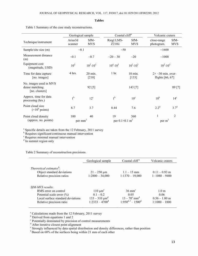
Table 1 Summary of the case study reconstructions.
a Specific details are taken from the 12 February, 2011 survey b Requires significant/continuous manual intervention c Requires minimal manual intervention d In summit region only
Table 2 Summary of reconstruction precisions. Geological sample Coastal cliff a Volcanic craters Theoretical estimatesb:
Object standard deviations 21 – 250 µm 1.1 – 15 mm 0.11 – 0.93 m Relative precision ratios 1:2800 – 34,000 1:1370 – 19,000 1: 1080 – 9400
SfM-MVS results:
RMS error on control 110 µmc 36 mmc 1.0 m Potential scale error (%) 0.1 – 0.2 0.05 0.06 Local surface standard deviations 133 – 310 µmd 13 – 70e mmd 0.56 – 1.00 m Relative precision ratio 1:2333 – 4700d 1:950d, f – 1500d 1:1000 – 1800
a Calculations made from the 12 February, 2011 survey b Derived from equations 1 and 2 c Potentially dominated by precision of control measurements d After iterative closest point alignment e Strongly influenced by data spatial distribution and density differences, rather than position f Based on 68% of the surfaces being within 21 mm of each other
Geological sample Coastal cliffa Volcanic craters
Technique/instrument Arius3d scanner
SfM- MVS
Riegl LMS-Z210ii
SfM- MVS
close-range photogram.
SfM-MVS
Sample/site size (m) ~0.1 ~50 ~1600
Measurement distance (m)
~0.1 ~0.7 ~20 – 30 ~20 ~1000
Equipment cost (magnitude, USD)
105 102-103 104-105 102-103 102-103
Time for data capture [no. images]
4 hrs.
20 min. [210]
1 hr.
10 min. [133]
2× ~30 min. over-flights [66, 67]
No. images used in MVS dense matching [no. clusters]
92 [5]
143 [7]
89 [7]
Approx. time for data processing (hrs.)
1b 12c 1b 10c 10b 14c
Point cloud size (×106 points)
8.7 3.7 0.44 7.6 2.2d 3.7d
Point cloud density (approx. no. points)
100 40 19 360 1 2
per mm2 per 0.1×0.1 m2 per m2
SfM-MVS
x = 0
y = 0
1231 2 3
y = 0
x = 0
c d
scanner
mm
0
50
mm
b
a
scannerSfM-MVS
Figure 01 James & Robson
radialdi�erence
Figure 1. Geological hand sample case study. (a) Example images used for the SfM-MVS reconstruction of the volcanic bomb sample, with insets (upper panel, 60×60 pixels) showing local image detail on the sample surface and (lower panel, 20×20 pixels) one of the marker dots used for scaling. (b) The camera positions (shown as cones) calculated by the SfM algorithm in the reconstruction coordinate system, encircling the sample. (c) Comparative views of the 3d models derived from the Arius scanner (upper panel) and the SfM-MVS approach (lower panel). Note that absolute colors/shadings should not be compared; no attempt has been made to ensure faithful color reproduction in either model. Both models are cut by planes for which the cross sections, represented by any points that fall within a distance of 0.1 mm of the plane, are overlain in (d). The quality of the SfM-MVS reconstruction can be seen by the good agreement to the data from the scanner. In the center of both cross sections, a plot of radial di�erence between the models is given (calculated as the average radius taken over a 1° arc for the SfM-MVS model, minus that of the scanner model), with the dashed circle representing zero di�erence. Note that the di�erences are plotted at a scale approximately an order of magnitude greater than that of the cross sections themselves (the di�erence scale is labeled in the lower panel only). Enlargements of two areas (~15 mm long) from the y = 0 section are shown in the insets.
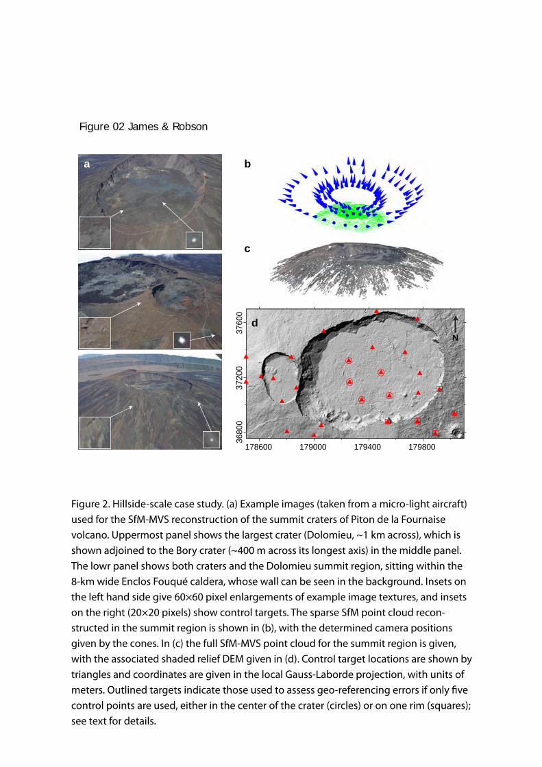
Figure 02 James & Robson
a b
c
d
178600 179000 179400 179800
3680
037
200
3760
0
N
Figure 2. Hillside-scale case study. (a) Example images (taken from a micro-light aircraft) used for the SfM-MVS reconstruction of the summit craters of Piton de la Fournaise volcano. Uppermost panel shows the largest crater (Dolomieu, ~1 km across), which is shown adjoined to the Bory crater (~400 m across its longest axis) in the middle panel. The lowr panel shows both craters and the Dolomieu summit region, sitting within the 8-km wide Enclos Fouqué caldera, whose wall can be seen in the background. Insets on the left hand side give 60×60 pixel enlargements of example image textures, and insets on the right (20×20 pixels) show control targets. The sparse SfM point cloud recon-structed in the summit region is shown in (b), with the determined camera positions given by the cones. In (c) the full SfM-MVS point cloud for the summit region is given, with the associated shaded relief DEM given in (d). Control target locations are shown by triangles and coordinates are given in the local Gauss-Laborde projection, with units of meters. Outlined targets indicate those used to assess geo-referencing errors if only �ve control points are used, either in the center of the crater (circles) or on one rim (squares); see text for details.
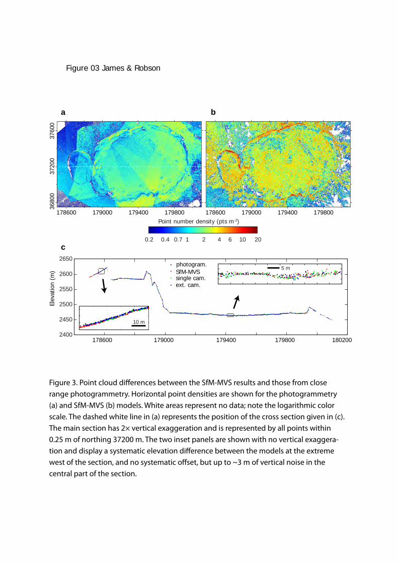
Point number density (pts m-2)
b
178600 179000 179400 179800
3680
037
200
3760
0
178600 179000 179400 179800
a
Figure 03 James & Robson
0.2 0.4 1 2 4 6 10 200.7
Elev
atio
n (m
)
c
Figure 3. Point cloud di�erences between the SfM-MVS results and those from close range photogrammetry. Horizontal point densities are shown for the photogrammetry (a) and SfM-MVS (b) models. White areas represent no data; note the logarithmic color scale. The dashed white line in (a) represents the position of the cross section given in (c). The main section has 2× vertical exaggeration and is represented by all points within 0.25 m of northing 37200 m. The two inset panels are shown with no vertical exaggera-tion and display a systematic elevation di�erence between the models at the extreme west of the section, and no systematic o�set, but up to ~3 m of vertical noise in the central part of the section.
2400
2450
2500
2550
2600
2650
178600 179000 179400 179800 180200
photogram.
ext. cam.
SfM-MVSsingle cam.
10 m
5 m
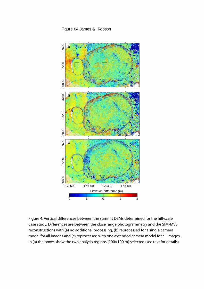
3680
037
200
3760
0 a
3680
037
200
3760
0 b
178600 179000 179400 179800
3680
037
200
3760
0 c
Figure 04 James & Robson
-1 0 1 2-2
Elevation difference (m)
Figure 4. Vertical di�erences between the summit DEMs determined for the hill-scale case study. Di�erences are between the close range photogrammetry and the SfM-MVS reconstructions with (a) no additional processing, (b) reprocessed for a single camera model for all images and (c) reprocessed with one extended camera model for all images. In (a) the boxes show the two analysis regions (100×100 m) selected (see text for details).
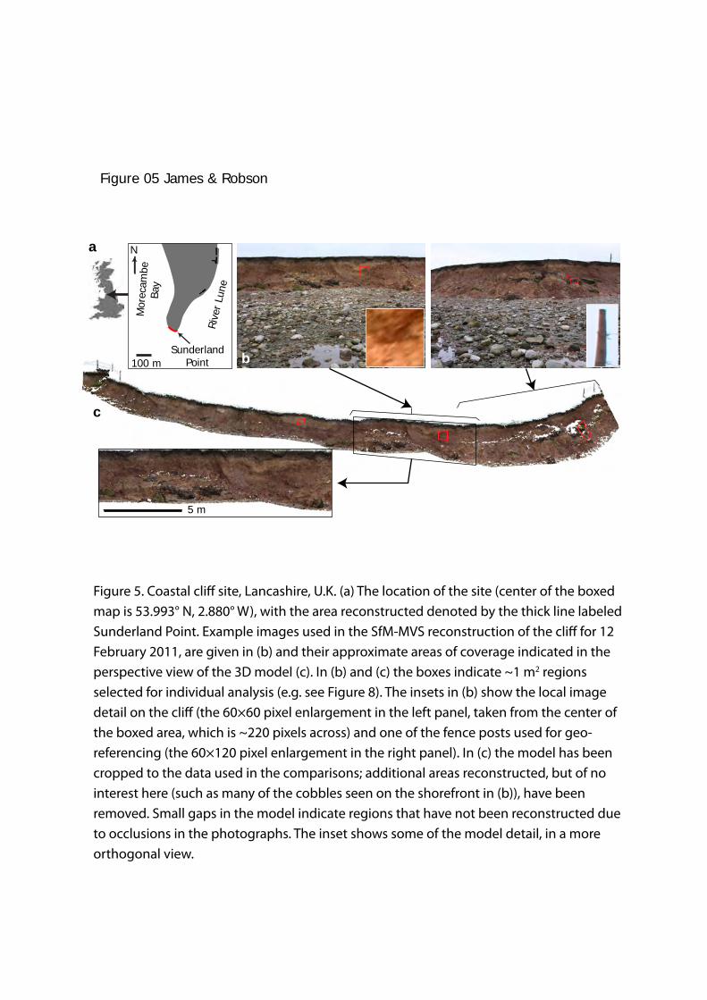
c
5 m
100 m
a
Mor
ecam
beBa
y
Rive
r Lu
ne
N
SunderlandPoint
Figure 05 James & Robson
b
Figure 5. Coastal cli� site, Lancashire, U.K. (a) The location of the site (center of the boxed map is 53.993° N, 2.880° W), with the area reconstructed denoted by the thick line labeled Sunderland Point. Example images used in the SfM-MVS reconstruction of the cli� for 12 February 2011, are given in (b) and their approximate areas of coverage indicated in the perspective view of the 3D model (c). In (b) and (c) the boxes indicate ~1 m2 regions selected for individual analysis (e.g. see Figure 8). The insets in (b) show the local image detail on the cli� (the 60×60 pixel enlargement in the left panel, taken from the center of the boxed area, which is ~220 pixels across) and one of the fence posts used for geo-referencing (the 60×120 pixel enlargement in the right panel). In (c) the model has been cropped to the data used in the comparisons; additional areas reconstructed, but of no interest here (such as many of the cobbles seen on the shorefront in (b)), have been removed. Small gaps in the model indicate regions that have not been reconstructed due to occlusions in the photographs. The inset shows some of the model detail, in a more orthogonal view.
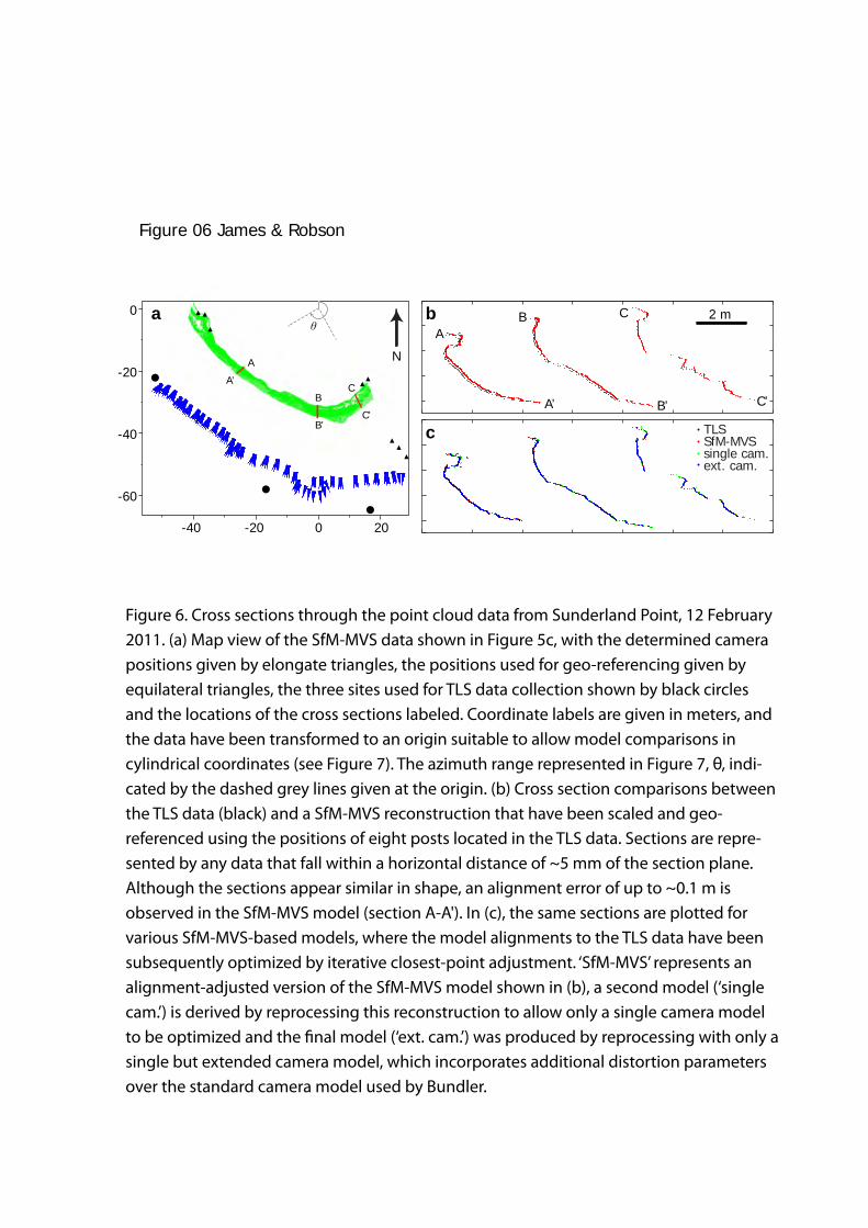
Figure 06 James & Robson
b
c
TLSSfM-MVSsingle cam.ext. cam.
C
C’
B
B’
A
A’
2 m
0 20-20-40
0
-20
-40
-60
a
C
C’
B
B’
A
A’
N
θ
Figure 6. Cross sections through the point cloud data from Sunderland Point, 12 February 2011. (a) Map view of the SfM-MVS data shown in Figure 5c, with the determined camera positions given by elongate triangles, the positions used for geo-referencing given by equilateral triangles, the three sites used for TLS data collection shown by black circles and the locations of the cross sections labeled. Coordinate labels are given in meters, and the data have been transformed to an origin suitable to allow model comparisons in cylindrical coordinates (see Figure 7). The azimuth range represented in Figure 7, θ, indi-cated by the dashed grey lines given at the origin. (b) Cross section comparisons between the TLS data (black) and a SfM-MVS reconstruction that have been scaled and geo-referenced using the positions of eight posts located in the TLS data. Sections are repre-sented by any data that fall within a horizontal distance of ~5 mm of the section plane. Although the sections appear similar in shape, an alignment error of up to ~0.1 m is observed in the SfM-MVS model (section A-A'). In (c), the same sections are plotted for various SfM-MVS-based models, where the model alignments to the TLS data have been subsequently optimized by iterative closest-point adjustment. ‘SfM-MVS’ represents an alignment-adjusted version of the SfM-MVS model shown in (b), a second model (‘single cam.’) is derived by reprocessing this reconstruction to allow only a single camera model to be optimized and the �nal model (‘ext. cam.’) was produced by reprocessing with only a single but extended camera model, which incorporates additional distortion parameters over the standard camera model used by Bundler.
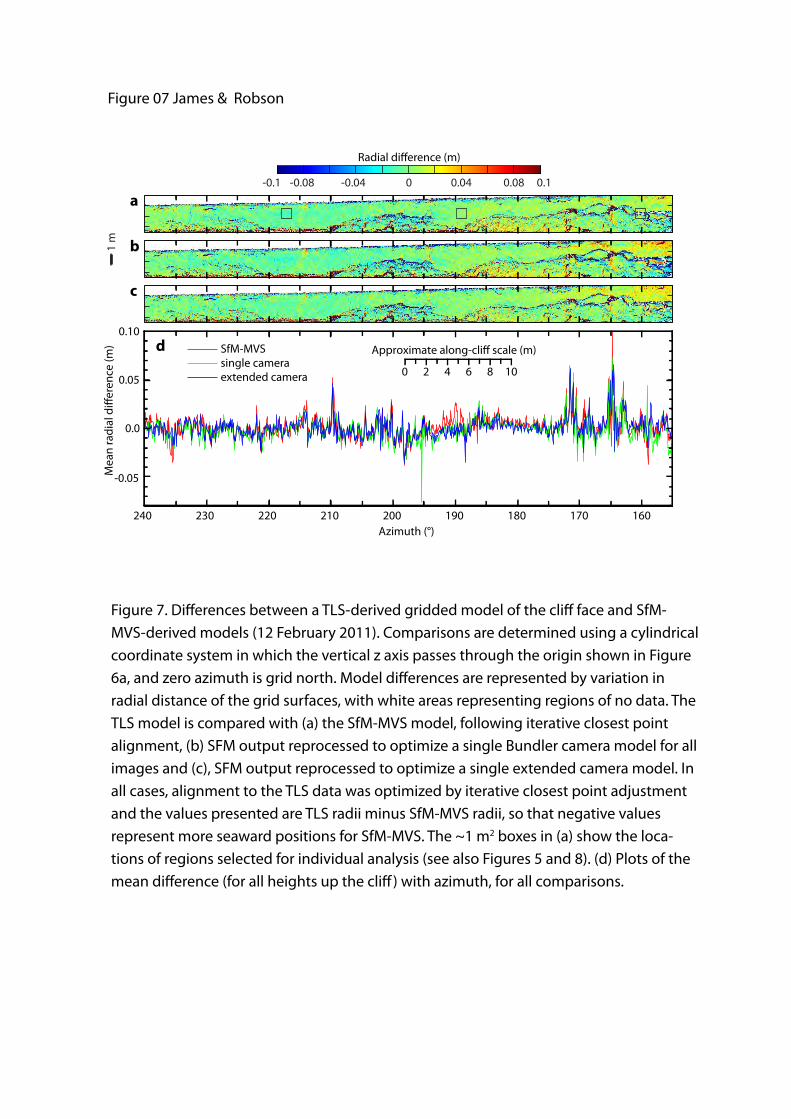
SfM-MVSsingle cameraextended camera
-0.05
0.0
0.05
0.10
240 230 220 210 200 190 180 170 160Azimuth (°)
Mea
n ra
dial
di�
eren
ce (m
) Approximate along-cli� scale (m)
0 2 4 6 8 10
1 m
a
b
c
-0.08 -0.04 0 0.04 0.08 0.1-0.1
Radial di�erence (m)
Figure 07 James & Robson
d
Figure 7. Di�erences between a TLS-derived gridded model of the cli� face and SfM-MVS-derived models (12 February 2011). Comparisons are determined using a cylindrical coordinate system in which the vertical z axis passes through the origin shown in Figure 6a, and zero azimuth is grid north. Model di�erences are represented by variation in radial distance of the grid surfaces, with white areas representing regions of no data. The TLS model is compared with (a) the SfM-MVS model, following iterative closest point alignment, (b) SFM output reprocessed to optimize a single Bundler camera model for all images and (c), SFM output reprocessed to optimize a single extended camera model. In all cases, alignment to the TLS data was optimized by iterative closest point adjustment and the values presented are TLS radii minus SfM-MVS radii, so that negative values represent more seaward positions for SfM-MVS. The ~1 m2 boxes in (a) show the loca-tions of regions selected for individual analysis (see also Figures 5 and 8). (d) Plots of the mean di�erence (for all heights up the cli�) with azimuth, for all comparisons.
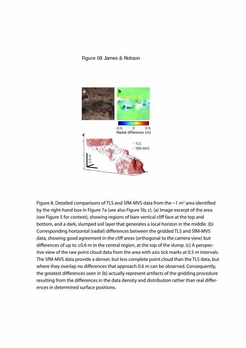
a b
c-0.6 0 0.6Radial difference (m)
Figure 08 James & Robson
0.5
m
TLSSfM-MVS
Figure 8. Detailed comparisons of TLS and SfM-MVS data from the ~1 m2 area identi�ed by the right-hand box in Figure 7a (see also Figure 5b, c). (a) Image excerpt of the area (see Figure 5 for context), showing regions of bare vertical cli� face at the top and bottom, and a dark, slumped soil layer that generates a local horizon in the middle. (b) Corresponding horizontal (radial) di�erences between the gridded TLS and SfM-MVS data, showing good agreement in the cli� areas (orthogonal to the camera view) but di�erences of up to ±0.6 m in the central region, at the top of the slump. (c) A perspec-tive view of the raw point cloud data from the area with axis tick marks at 0.5 m intervals. The SfM-MVS data provide a denser, but less complete point cloud than the TLS data, but where they overlap no di�erences that approach 0.6 m can be observed. Consequently, the greatest di�erences seen in (b) actually represent artifacts of the gridding procedure resulting from the di�erences in the data density and distribution rather than real di�er-ences in determined surface positions.
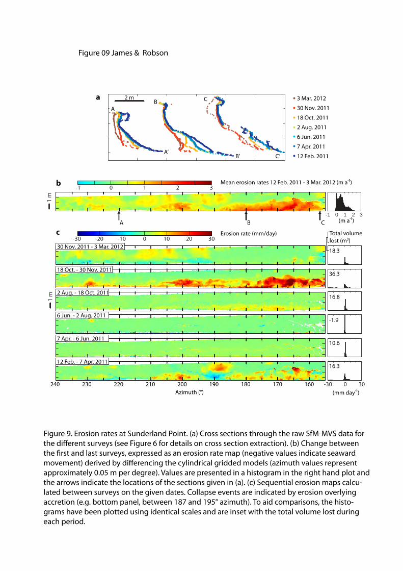
240 230 220 210 200 190 180 170 160Azimuth (°)
18 Oct. 2011
3 Mar. 2012
30 Nov. 2011
2 Aug. 2011
6 Jun. 2011
1 m
c
a
-20 -10 0 10 20 30-30Erosion rate (mm/day)
Figure 09 James & Robson
2 m
A
A’
B
B’
C
C’
A B C
0 30-30
Total volumelost (m3)
Figure 9. Erosion rates at Sunderland Point. (a) Cross sections through the raw SfM-MVS data for the di�erent surveys (see Figure 6 for details on cross section extraction). (b) Change between the �rst and last surveys, expressed as an erosion rate map (negative values indicate seaward movement) derived by di�erencing the cylindrical gridded models (azimuth values represent approximately 0.05 m per degree). Values are presented in a histogram in the right hand plot and the arrows indicate the locations of the sections given in (a). (c) Sequential erosion maps calcu-lated between surveys on the given dates. Collapse events are indicated by erosion overlying accretion (e.g. bottom panel, between 187 and 195° azimuth). To aid comparisons, the histo-grams have been plotted using identical scales and are inset with the total volume lost during each period.
1 m
7 Apr. 2011
12 Feb. 2011
30 Nov. 2011 - 3 Mar. 2012
18 Oct. - 30 Nov. 2011
2 Aug. - 18 Oct. 2011
6 Jun. - 2 Aug. 2011
7 Apr. - 6 Jun. 2011
12 Feb. - 7 Apr. 2011
b1 2 30
Mean erosion rates 12 Feb. 2011 - 3 Mar. 2012 (m a-1)-1
0 1 2 3-1(m a-1)
(mm day-1)
18.3
36.3
-1.9
16.8
10.6
16.3
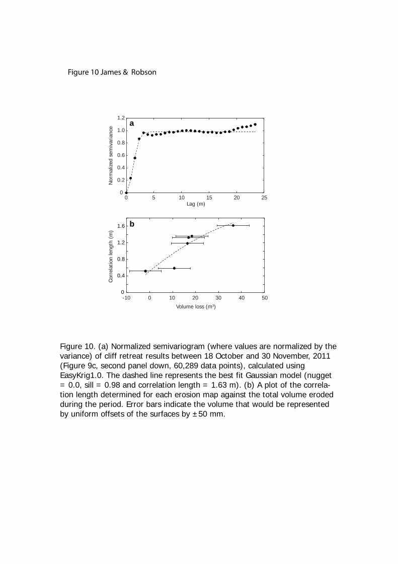
0
0.4
0.8
1.2
1.6
Volume loss (m3)
Corr
elat
ion
leng
th (
m)
b
0 10 20 30 40 50-10
0 5 10 15 20 250
0.2
0.4
0.6
0.8
1.0
1.2N
orm
aliz
ed s
emiv
aria
nce
Lag (m)
a
Figure 10. (a) Normalized semivariogram (where values are normalized by the variance) of cliff retreat results between 18 October and 30 November, 2011 (Figure 9c, second panel down, 60,289 data points), calculated using EasyKrig1.0. The dashed line represents the best fit Gaussian model (nugget = 0.0, sill = 0.98 and correlation length = 1.63 m). (b) A plot of the correla-tion length determined for each erosion map against the total volume eroded during the period. Error bars indicate the volume that would be represented by uniform offsets of the surfaces by ±50 mm.
Figure 10 James & Robson


![Implicit Meshes for Surface Reconstruction...patches [11], [21], and subdivision surfaces [16], [23], to unorganized 3D data. They are typically used to reconstruct surfaces from relatively](https://img.pdfslide.us/doc/110x75/5ed27fd7ad716a665e6d914f/implicit-meshes-for-surface-reconstruction-patches-11-21-and-subdivision.jpg)