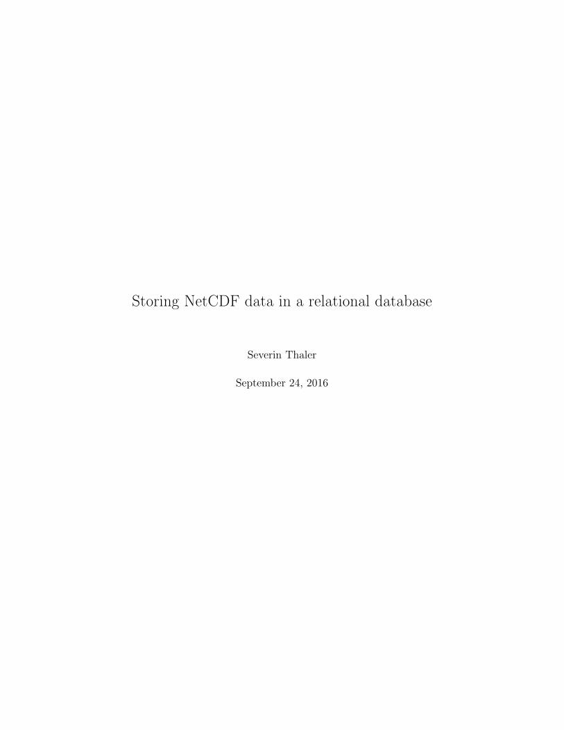
Storing NetCDF data in a relational database

Severin Thaler

September 24, 2016

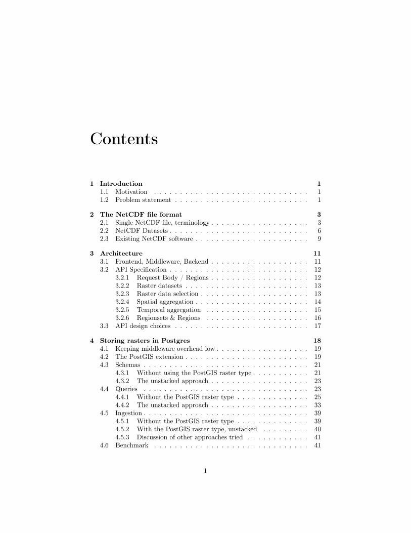
Contents

1 Introduction 11.1 Motivation . . . . . . . . . . . . . . . . . . . . . . . . . . . . . . 11.2 Problem statement . . . . . . . . . . . . . . . . . . . . . . . . . . 1

2 The NetCDF file format 32.1 Single NetCDF file, terminology . . . . . . . . . . . . . . . . . . . 32.2 NetCDF Datasets . . . . . . . . . . . . . . . . . . . . . . . . . . . 62.3 Existing NetCDF software . . . . . . . . . . . . . . . . . . . . . . 9

3 Architecture 113.1 Frontend, Middleware, Backend . . . . . . . . . . . . . . . . . . . 113.2 API Specification . . . . . . . . . . . . . . . . . . . . . . . . . . . 12

3.2.1 Request Body / Regions . . . . . . . . . . . . . . . . . . . 123.2.2 Raster datasets . . . . . . . . . . . . . . . . . . . . . . . . 133.2.3 Raster data selection . . . . . . . . . . . . . . . . . . . . . 133.2.4 Spatial aggregation . . . . . . . . . . . . . . . . . . . . . . 143.2.5 Temporal aggregation . . . . . . . . . . . . . . . . . . . . 153.2.6 Regionsets & Regions . . . . . . . . . . . . . . . . . . . . 16

3.3 API design choices . . . . . . . . . . . . . . . . . . . . . . . . . . 17

4 Storing rasters in Postgres 184.1 Keeping middleware overhead low . . . . . . . . . . . . . . . . . . 194.2 The PostGIS extension . . . . . . . . . . . . . . . . . . . . . . . . 194.3 Schemas . . . . . . . . . . . . . . . . . . . . . . . . . . . . . . . . 21

4.3.1 Without using the PostGIS raster type . . . . . . . . . . . 214.3.2 The unstacked approach . . . . . . . . . . . . . . . . . . . 23

4.4 Queries . . . . . . . . . . . . . . . . . . . . . . . . . . . . . . . . 234.4.1 Without the PostGIS raster type . . . . . . . . . . . . . . 254.4.2 The unstacked approach . . . . . . . . . . . . . . . . . . . 33

4.5 Ingestion . . . . . . . . . . . . . . . . . . . . . . . . . . . . . . . . 394.5.1 Without the PostGIS raster type . . . . . . . . . . . . . . 394.5.2 With the PostGIS raster type, unstacked . . . . . . . . . 404.5.3 Discussion of other approaches tried . . . . . . . . . . . . 41

4.6 Benchmark . . . . . . . . . . . . . . . . . . . . . . . . . . . . . . 41

1

4.6.1 Setup . . . . . . . . . . . . . . . . . . . . . . . . . . . . . 414.6.2 Results . . . . . . . . . . . . . . . . . . . . . . . . . . . . 44

4.7 A more general API and Postgres schema . . . . . . . . . . . . . 484.7.1 A more general Postgres schema . . . . . . . . . . . . . . 494.7.2 A more general HTTP API . . . . . . . . . . . . . . . . . 54

2

Abstract

Climate science requires the analysis of variables such as temperature, precipi-tation, and ozone concentration, which depend on multiple dimensions, mainlytime, latitude, longitude, and height/depth, and are commonly stored in theNetCDF file format. Various infrastructure has evolved around this formatsuch as libraries, command line tools, visualization software, and web services.In this work we present a prototype for serving NetCDF data backed by theopen-source RDBMS Postgres. We test various database schemas in the searchfor one that delivers response times low enough for visualization and furthersupports the diversity present among NetCDF files.

Chapter 1

Introduction

1.1 MotivationIn climate science one studies variables such as temperature which depend onmultiple dimensions, most notably time, latitude, longitude, and height/depth(or short vertical). This data comes from actual measurements obtained fromweather stations or satellites or from a simulation and is often stored in theNetCDF file format. Common tasks performed on climate variables are subset-ting (i.e. retrieving a spatio-temporal subset of a variable’s data), computingsummary statistics (i.e. aggregating a variable along a dimension using an op-eration like sum or average), and visualization. Subsetting is important fordrilling down a variable’s data to spatial regions and/or time/vertical ranges.Summary statistics provide information about the statistical distribution of avariable along dimensions. Visualization helps to identify extrema or generallypoints of interest in space-time in a quick ad-hoc fashion. All these operationsare of great help for analyzing climate data.Especially nowadays where policy makers and the public are increasingly con-cerned about climate change, efficient tools that support these operations willbe of great need and impact. The purpose of this work is to present a prototypefor such a tool, a retrieval service for NetCDF data with a focus on providingresponse times low enough for a visualization frontend application.When it comes to the design of such a tool several decisions need to be made, inparticular how the data retrieval API shall look like and how the data shall bestored. In this work we discuss these decisions and pave the way for an advancedfuture climate data access service along with a visualization frontend.

1.2 Problem statementThe problem this work addresses is how to store NetCDF data in a relationaldatabase using an appropriate schema and design a data access API on top ofthat, with a focus on providing response times low enough for visualization pur-

1

poses. Moreover, we also propose a generalized schema able to accommodatemore diverse NetCDF files. In doing so we gain an understanding of how ap-propriate a relational database is for NetCDF data with its multi-dimensionalcharacter.

2

Chapter 2

The NetCDF file format

The NetCDF file format is a generic file format to accommodate multi-dimensionaldata. A NetCDF file consists of dimensions, variables that depend on dimen-sions, and attributes which can be associated to variables or to the NetCDF fileas a whole. A variable’s data is stored as a flat array in row-major order of thedimensions it depends on. NetCDF I/O libraries in various languages provideconvenient APIs to read/write NetCDF files. From a superficial point of viewthe NetCDF format seems quite straightforward. However, because it is still ageneric format, conventions are needed to impose further structure which canthen be assumed/exploited by applications. In this respect, the CF conventionshave become the de facto standard. This chapter will clarify some terminologyand lay the groundwork for subsequent chapters.

2.1 Single NetCDF file, terminologyIn this section we familiarize ourselves with the structure of a NetCDF file.

As an example, let us consider a NetCDF file produced by the parallel Systemfor Integrating Impact Models and Sectors (pSIMS) [Elliott2014509]. Listing2.1 shows the contents of such a file obtained through the command ncdump-c, where ncdump is a NetCDF command line utility.

3

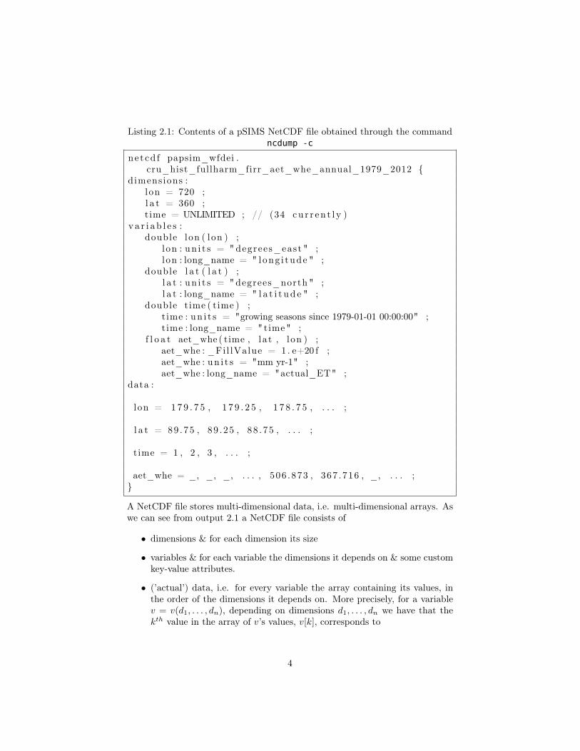
Listing 2.1: Contents of a pSIMS NetCDF file obtained through the commandncdump -c

netcd f papsim_wfdei .cru_hist_fullharm_firr_aet_whe_annual_1979_2012 {

dimensions :lon = 720 ;l a t = 360 ;time = UNLIMITED ; // (34 cu r r en t l y )

v a r i a b l e s :double lon ( lon ) ;

lon : un i t s = " degrees_east " ;lon : long_name = " long i tude " ;

double l a t ( l a t ) ;l a t : un i t s = "degrees_north " ;l a t : long_name = " l a t i t u d e " ;

double time ( time ) ;time : un i t s = "growing seasons since 1979-01-01 00:00:00" ;time : long_name = "time" ;

f l o a t aet_whe ( time , l a t , lon ) ;aet_whe : _Fil lValue = 1 . e+20 f ;aet_whe : un i t s = "mm yr-1" ;aet_whe : long_name = "actual_ET" ;

data :

lon = 17 9 . 7 5 , 1 7 9 . 2 5 , 1 7 8 . 7 5 , . . . ;

l a t = 89 .75 , 89 . 25 , 88 . 75 , . . . ;

time = 1 , 2 , 3 , . . . ;

aet_whe = _, _, _, . . . , 506 .873 , 367 .716 , _, . . . ;}

A NetCDF file stores multi-dimensional data, i.e. multi-dimensional arrays. Aswe can see from output 2.1 a NetCDF file consists of

• dimensions & for each dimension its size

• variables & for each variable the dimensions it depends on & some customkey-value attributes.

• (’actual’) data, i.e. for every variable the array containing its values, inthe order of the dimensions it depends on. More precisely, for a variablev = v(d1, . . . , dn), depending on dimensions d1, . . . , dn we have that thekth value in the array of v’s values, v[k], corresponds to

4

v(i1, . . . , in),

where

i1 × s2 × · · · sn + . . .+ in−2 × sn−1 × sn + in−1 × sn + in := k,

with si being the size of dimension di and 0 ≤ ik < sk.In other words, a variable’s data is stored in row-major order of its dimen-sions.

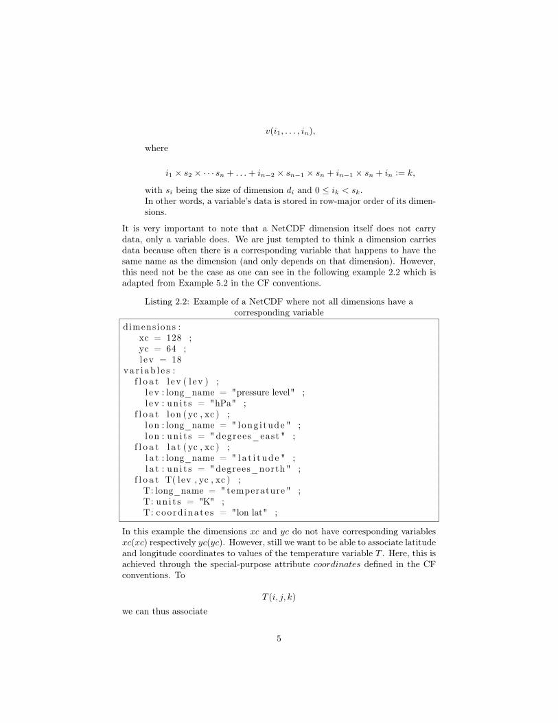
It is very important to note that a NetCDF dimension itself does not carrydata, only a variable does. We are just tempted to think a dimension carriesdata because often there is a corresponding variable that happens to have thesame name as the dimension (and only depends on that dimension). However,this need not be the case as one can see in the following example 2.2 which isadapted from Example 5.2 in the CF conventions.

Listing 2.2: Example of a NetCDF where not all dimensions have acorresponding variable

dimensions :xc = 128 ;yc = 64 ;l ev = 18

va r i a b l e s :f l o a t l ev ( l ev ) ;

l e v : long_name = "pressure level" ;l e v : un i t s = "hPa" ;

f l o a t lon ( yc , xc ) ;lon : long_name = " long i tude " ;lon : un i t s = " degrees_east " ;

f l o a t l a t ( yc , xc ) ;l a t : long_name = " l a t i t u d e " ;l a t : un i t s = "degrees_north " ;

f l o a t T( lev , yc , xc ) ;T: long_name = " temperature " ;T: un i t s = "K" ;T: coo rd ina t e s = "lon lat" ;

In this example the dimensions xc and yc do not have corresponding variablesxc(xc) respectively yc(yc). However, still we want to be able to associate latitudeand longitude coordinates to values of the temperature variable T . Here, this isachieved through the special-purpose attribute coordinates defined in the CFconventions. To

T (i, j, k)

we can thus associate

5

lev(i)lat(j, k)lon(j, k)

and therefore geo-locate the temperature values. Before the CF conventionsappeared with this special-purpose coordinates attribute the COARDS con-ventions dominated. Those however only had one means to associate to a vari-able other variables with geo-locating information, namely, as mentioned earlier,through variables that have the same names as dimensions. This is the case forthe pSIMS file 2.1 where to

aet_whe(i, j, k)

we can associate

time(i)lat(j)lon(k)

Note that the variable lev in example 2.2 is linked to the T variable in this waytoo, it is only the lat, lon variables which are linked through T ’s special-purposecoordinates attribute.We thus realize that some NetCDF variables take on a special role in that theycarry temporal or spatial information, i.e. time, vertical (i.e. height/depth,but also pressure since pressure basically encodes a height/depth), latitude, orlongitude. Such variables are used to reference other variables in space andtime. In accordance with the CF conventions we call such variables coordinatevariables respectively auxiliary coordinate variables (see the CF conventions forprecise definitions). The CF conventions give clear rules to detect time, vertical,latitude, longitude variables, basically via the units attribute.

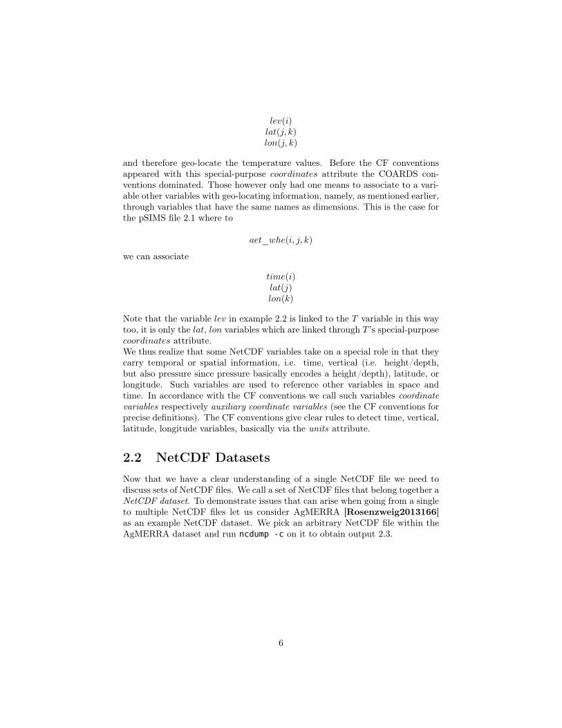
2.2 NetCDF DatasetsNow that we have a clear understanding of a single NetCDF file we need todiscuss sets of NetCDF files. We call a set of NetCDF files that belong together aNetCDF dataset. To demonstrate issues that can arise when going from a singleto multiple NetCDF files let us consider AgMERRA [Rosenzweig2013166]as an example NetCDF dataset. We pick an arbitrary NetCDF file within theAgMERRA dataset and run ncdump -c on it to obtain output 2.3.

6

Listing 2.3: Output of ncdump -c on some AgMERRA NetCDF file

ne tcd f clim_0007_0056 . t i l e {dimensions :

l a t = 8 ;lon = 8 ;time = UNLIMITED ; // (11323 cu r r en t l y )

v a r i a b l e s :f l o a t pr ( time , l a t , lon ) ;

pr : standard_name = " p r e c i p i t a t i o n_ f l ux " ;pr : long_name = "Precipitation Flux" ;pr : un i t s = "kg m-2 s-1" ;pr : _Fi l lValue = 1 . e+20 f ;. . .

f l o a t cropland ( la t , lon ) ;cropland : un i t s = "percent" ;cropland : long_name = "cropland" ;

// g l oba l a t t r i b u t e s ::CDI = "Climate Data Interface version 1.6.8 ..." ;: Conventions = "CF-1.4" ;: history = "Thu Aug 13 14:40:20 2015: cdo ..." ;: t i t l e = "AgMERRA Relative Humidity at time of ..." ;: c en t e r = "NASA GISS" ;: comment = "AgMERRA dataset processed for ISI-MIP, ..." ;:CDO = "Climate Data Operators version 1.6.8 ..." ;: source = "AgMIP / Alex Ruane" ;

data :

l a t = 77 .875 , 77 .625 , 77 .375 , . . . , 76 .125 ;

lon = 69 . 8 7 5 , 6 9 . 6 2 5 , 6 9 . 3 7 5 , . . . , 6 8 . 1 2 5 ;

time = 43829.0416666667 , 43830.0416666667 ,43831.0416666667 , . . . , 55151.0416666667 ;

}

For the sake of brevity we left out some variables and shortened some globalattributes. Important is that each individual NetCDF file only covers an 8x8 tileof the entire spatial extent and code that processes these NetCDF files must beintelligent enough to realize that. In particular it mustn’t consider variables indifferent NetCDF files to be different actually, they represent the same variablejust covering different spatial extents.We note that tiling is not the only way NetCDF files can split a dataset. Adataset can also be split along time, e.g. every NetCDF file can cover a dayof hourly data. It can also be split ”by variable” by which we mean that every

7

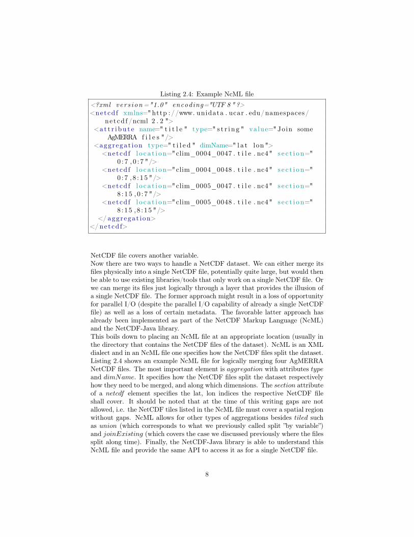
Listing 2.4: Example NcML file

<?xml ve r s i on ="1.0" encoding="UTF 8 " ?><netcd f xmlns="http ://www. unidata . ucar . edu/namespaces/

ne tcd f /ncml 2 . 2 "><a t t r i bu t e name=" t i t l e " type=" s t r i n g " value="Join some

AgMERRA f i l e s "/><aggregat ion type=" t i l e d " dimName=" l a t lon ">

<netcd f l o c a t i o n="clim_0004_0047 . t i l e . nc4" s e c t i o n="0 : 7 , 0 : 7 "/>

<netcd f l o c a t i o n="clim_0004_0048 . t i l e . nc4" s e c t i o n="0 : 7 , 8 : 1 5 "/>

<netcd f l o c a t i o n="clim_0005_0047 . t i l e . nc4" s e c t i o n="8 : 1 5 , 0 : 7 "/>

<netcd f l o c a t i o n="clim_0005_0048 . t i l e . nc4" s e c t i o n="8 : 15 , 8 : 1 5 "/>

</ aggregat ion></ netcd f>

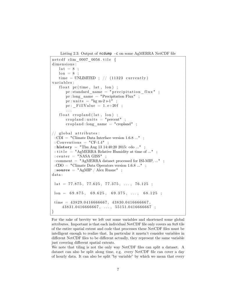
NetCDF file covers another variable.Now there are two ways to handle a NetCDF dataset. We can either merge itsfiles physically into a single NetCDF file, potentially quite large, but would thenbe able to use existing libraries/tools that only work on a single NetCDF file. Orwe can merge its files just logically through a layer that provides the illusion ofa single NetCDF file. The former approach might result in a loss of opportunityfor parallel I/O (despite the parallel I/O capability of already a single NetCDFfile) as well as a loss of certain metadata. The favorable latter approach hasalready been implemented as part of the NetCDF Markup Language (NcML)and the NetCDF-Java library.This boils down to placing an NcML file at an appropriate location (usually inthe directory that contains the NetCDF files of the dataset). NcML is an XMLdialect and in an NcML file one specifies how the NetCDF files split the dataset.Listing 2.4 shows an example NcML file for logically merging four AgMERRANetCDF files. The most important element is aggregation with attributes typeand dimName. It specifies how the NetCDF files split the dataset respectivelyhow they need to be merged, and along which dimensions. The section attributeof a netcdf element specifies the lat, lon indices the respective NetCDF fileshall cover. It should be noted that at the time of this writing gaps are notallowed, i.e. the NetCDF tiles listed in the NcML file must cover a spatial regionwithout gaps. NcML allows for other types of aggregations besides tiled suchas union (which corresponds to what we previously called split ”by variable”)and joinExisting (which covers the case we discussed previously where the filessplit along time). Finally, the NetCDF-Java library is able to understand thisNcML file and provide the same API to access it as for a single NetCDF file.

8

2.3 Existing NetCDF softwareIn this section we give a brief overview of existing NetCDF-related software witha focus on NetCDF data access services.

On a low level there are of course libraries for reading and writing NetCDFfiles in various languages such as C/C++ (GDAL), Java (NetCDF-Java), andPython (netCDF4-python). Just like any object-oriented I/O library for a fileformat these libraries provide classes that reflect the data model of the file for-mat. When working with such a library, or any I/O library for any file format inthis regard, it is important to understand its I/O behavior, i.e. when bytes areactually read/written and how many, especially because of lazy loading seman-tics. As already mentioned in the previous section, NetCDF-Java provides goodsupport for NetCDF datasets through the NetCDF Markup Language (NcML).The netCDF4-python library offers similar support through the MFDatasetclass, however, this currently only works for the NetCDF3 and NetCDF4-classicformats.

On a higher level we have the OPeNDAP standard. It is a data access protocolmost notably used for but not limited to NetCDF data. OPeNDAP definesan HTTP API for clients to access the data without prescribing how that datashould actually be stored, i.e. whether the data is stored as files or in a databasedoes not matter. The DAP specification (currently at version 2.0) allows forsubsetting a variable’s data by restricting the range of its dimensions both byindex but actually also by value, since indexes alone are not user-friendly. Aprominent DAP implementation is the Hyrax server. As mentioned, the DAPstandard is agnostic about how the data is actually stored. If however, onedecides to store the data in a relational database then a mapping is requiredfrom the DAP HTTP requests to SQL queries and thus also a mapping from theDAP data model to the relational model. For Hyrax this is achieved by writinga plug-in relational database handler module for the backend server (BES). Thework described in this document basically fits in there, i.e. it presents a proto-type for storing NetCDF data in a relational database and an HTTP API ontop of that, from scratch. As a shortcut we could have written a BES moduleinstead.On a slightly higher level there is the NetCDF Subset Service (NCSS) whichsimplifies the subsetting of NetCDF variables along the common time, vertical,latitude, and longitude coordinates.There is also the proprietary ArcGIS Server to which one can register data inboth files and databases too.

Since in the present work we design the data access API and the backend witha focus on satisfying the needs of a visualization application, it makes senseto look at existing NetCDF visualization software. Notably there is for in-stance Panoply. Its strengths are that it can detect a variable’s latitude andlongitude variables by means of the CF conventions. Moreover, it can read re-

9

mote THREDDS and OPeNDAP catalogs and can in particular handle NetCDFdatasets since it uses NetCDF-Java underneath which understands NcML. How-ever, it is on-premise as opposed to SaaS. Further, while it does a good job atdetecting and offering special support for latitude, longitude variables it doesvery little to offer special support for time and vertical variables. While it is atleast able to display human-readable timestamps in case of a time variable itdoesn’t treat a vertical variable different from a time variable in the sense thatboth are presented to the user as sliders on which one can select a specific verti-cal position respectively point in time (selecting an interval of vertical positionsrespectively times though is not possible). Best would be to present the verticalvariable separately from the time variable in the form of an extra height bar onthe plotted map.

On a storage backend level it seems the most common approach is to just keepthe data in NetCDF files. This also seems to be the case for Hyrax though itdoes allow for storing the data in a relational database too. A third approach isto use a so-called array database such as Rasdaman, SciDB, or MonetDB. How-ever, MonetDB is in fact a column-oriented relational database and Rasdamanis often deployed with Postgres as the underlying storage backend (though itcan also use the filesystem directly) in which case an array’s tiles end up asBLOB rows in Postgres. MonetDB’s array query language is SciQL and Ras-daman’s is RasQL. After a SciQL query is compiled to an execution plan itsleaves ultimately operate on the storage layout of a column-oriented relationaldatabase. After a RasQL query is compiled to an execution plan, and assumingPostgres is set as the underlying storage system, its leaves access the data fromPostgres (using ordinary SQL queries).For the present work we decided to base our prototype on the established Post-gres database. The discussion whether to use an array database or even whetherto use a database in the first place as opposed to just NetCDF files is a discussionin its own right.

10

Chapter 3

Architecture

In this chapter we describe the components of our prototype all the way fromthe user’s browser to the Postgres database. Further, we specify the HTTPendpoints of our NetCDF data access API, i.e. format of URL, request body (ifthe HTTP method on the respective route allows for a body), and response.

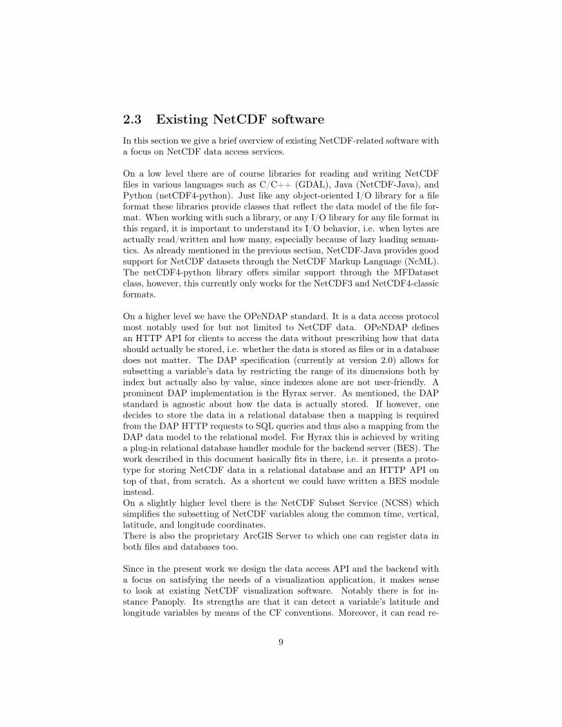
3.1 Frontend, Middleware, BackendFigure 3.1 shows the overall architecture of the prototype.

Figure 3.1: Overall architecture of the prototype

A client’s web browser issues an HTTP request which first arrives at the nginxweb server. nginx is used to serve static content like CSS, JavaScript, and im-ages, and caches this content. Requests for dynamic content are forwarded bynginx to uWSGI through the uwsgi protocol. The uWSGI web server’s workerprocesses execute Python Flask code (via linking libpython.so). There are twoFlask codes. One that serves dynamic HTML and is part of the ATLAS Viewerproject which also contains the JavaScript code. This project implements thewebpage that visualizes our NetCDF data. The other Flask code is our NetCDFdata access API which we named EDE (Environmental Discovery Engine) when

11

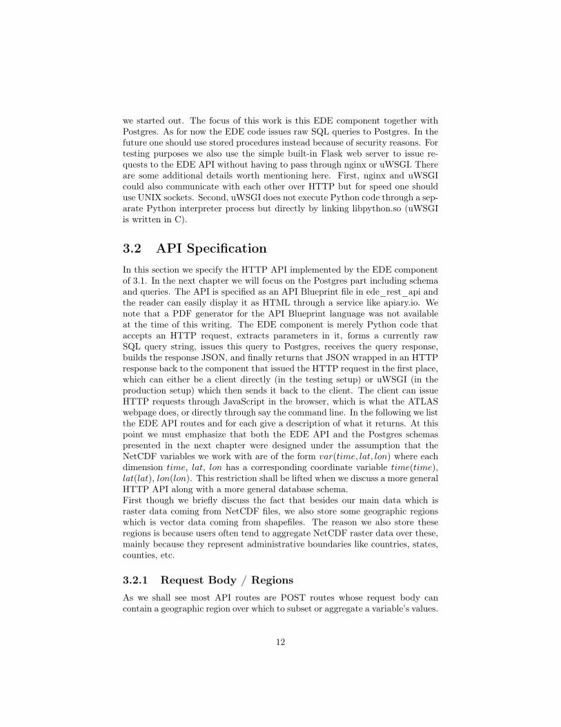
we started out. The focus of this work is this EDE component together withPostgres. As for now the EDE code issues raw SQL queries to Postgres. In thefuture one should use stored procedures instead because of security reasons. Fortesting purposes we also use the simple built-in Flask web server to issue re-quests to the EDE API without having to pass through nginx or uWSGI. Thereare some additional details worth mentioning here. First, nginx and uWSGIcould also communicate with each other over HTTP but for speed one shoulduse UNIX sockets. Second, uWSGI does not execute Python code through a sep-arate Python interpreter process but directly by linking libpython.so (uWSGIis written in C).

3.2 API SpecificationIn this section we specify the HTTP API implemented by the EDE componentof 3.1. In the next chapter we will focus on the Postgres part including schemaand queries. The API is specified as an API Blueprint file in ede_rest_api andthe reader can easily display it as HTML through a service like apiary.io. Wenote that a PDF generator for the API Blueprint language was not availableat the time of this writing. The EDE component is merely Python code thataccepts an HTTP request, extracts parameters in it, forms a currently rawSQL query string, issues this query to Postgres, receives the query response,builds the response JSON, and finally returns that JSON wrapped in an HTTPresponse back to the component that issued the HTTP request in the first place,which can either be a client directly (in the testing setup) or uWSGI (in theproduction setup) which then sends it back to the client. The client can issueHTTP requests through JavaScript in the browser, which is what the ATLASwebpage does, or directly through say the command line. In the following we listthe EDE API routes and for each give a description of what it returns. At thispoint we must emphasize that both the EDE API and the Postgres schemaspresented in the next chapter were designed under the assumption that theNetCDF variables we work with are of the form var(time, lat, lon) where eachdimension time, lat, lon has a corresponding coordinate variable time(time),lat(lat), lon(lon). This restriction shall be lifted when we discuss a more generalHTTP API along with a more general database schema.First though we briefly discuss the fact that besides our main data which israster data coming from NetCDF files, we also store some geographic regionswhich is vector data coming from shapefiles. The reason we also store theseregions is because users often tend to aggregate NetCDF raster data over these,mainly because they represent administrative boundaries like countries, states,counties, etc.

3.2.1 Request Body / RegionsAs we shall see most API routes are POST routes whose request body cancontain a geographic region over which to subset or aggregate a variable’s values.

12

A geographic region is basically a polygon and can be specified either directlyor indirectly. By directly we mean that the region’s polygon is specified inthe request body itself whereas by indirectly we mean that the request bodycontains a unique identifier which points to the region’s polygon stored in thedatabase itself. Among regions we store in the database itself are GADM (GlobalAdministrative Areas) regions because users often want to subset/aggregate avariable over such regions. The direct way of specifying a region is in particularused by ATLAS’ JavaScript code to restrict a variable’s data to a D3 boundingbox.Similar to the notion of a NetCDF dataset we also use the notion of a regionset,i.e. a set of regions. GADM is an example of a regionset we will be using mostlybut also EEZ (Exclusive Economic Zones) which are sea zones prescribed bythe United Nations Conventions on the Law of the Sea which regulates theexploitation and exploration of marine resources. In the longer term we couldalso allow users to create their own regionsets for custom repeating analysis.

3.2.2 Raster datasetsShow all datasets

GET /rastermeta

Return all NetCDF datasets currently stored in the backend, with associatedmetadata such as name, global attributes, etc.

Show a specific dataset

GET /rastermeta/dataset/dataset_id

Return a single NetCDF dataset currently stored in the backend, with its meta-data.

3.2.3 Raster data selectionFor a time range

POST /rasterdata/dataset/dataset_id/var/var_id/time/time_id_start:time_id_step:time_id_end

For variable var_id (depending on (time,lat,lon), i.e. v(time,lat,lon)) in datasetdataset_id return

v(i, j, k)

where

i ∈ [B,B+ S,B+ 2S, . . . ,E]

13

lat

lon

time

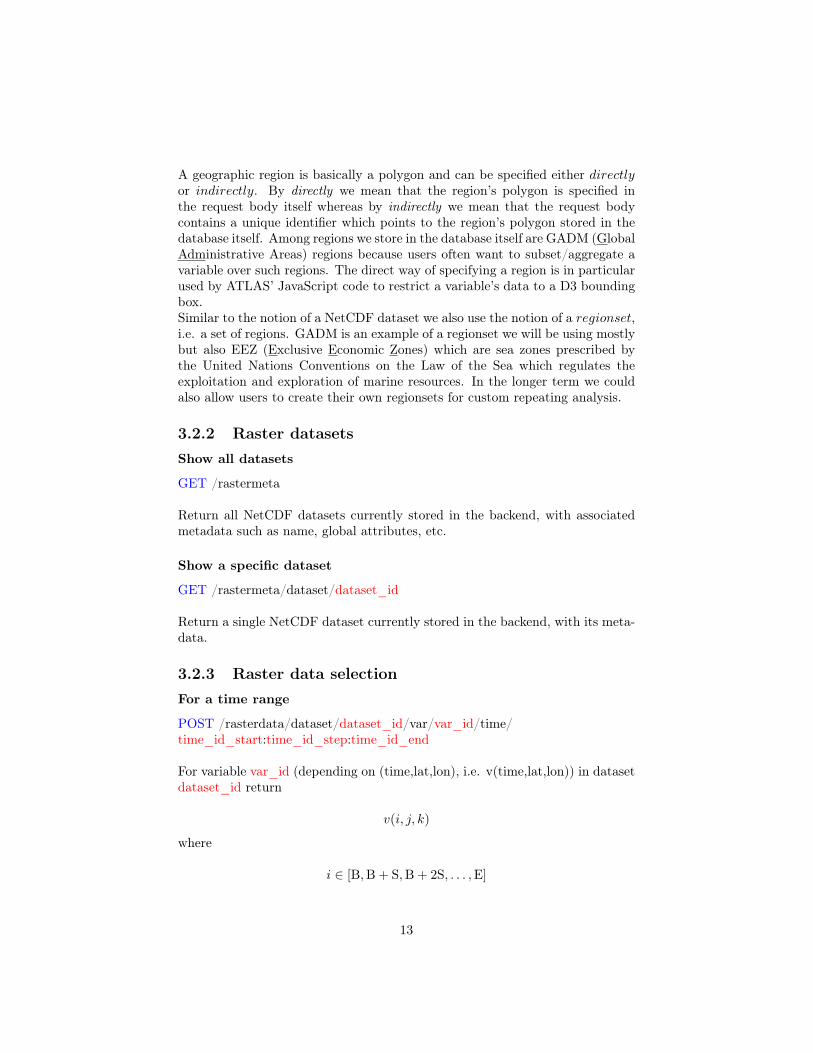
Figure 3.2: Illustration of the selection route

with B/S/E := time_id_start/step/end and

(lat(j), lon(k))

is within the region specified in the request body. This is just slicing a variablewith a range restriction on the time dimension (with gaps allowed) and a regionrestriction on (latitude,longitude). A visualization is given in Figure 3.2 wherethe cell centers illustrate the locations (lat(j), lon(k)). The blue polygon is thepolygon specified in the request body and the route returns all raster cells whosecenters lie inside the polygon (these cells are colored red), and this is done forall timesteps the user specifies (4 timesteps in case of the Figure).

For a specific time

POST /rasterdata/dataset/dataset_id/var/var_id/time/time_id

Same as previous route except that the variable’s time dimension is restrictedto a single time as opposed to a range of times.

3.2.4 Spatial aggregationFor a time range

POST /aggregate/spatial/dataset/dataset_id/var/var_id/time/time_id_start:time_id_step:time_id_end

For variable var_id in dataset dataset_id return

14

lat

lon

time

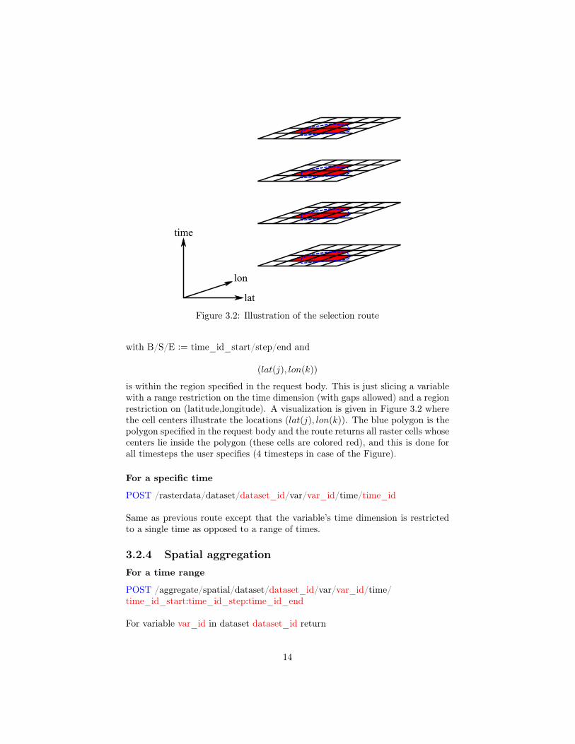
Figure 3.3: Illustration of the spatial aggregation route

op(lat(j),lon(k))∈R

v(i, j, k)

where

i ∈ [B,B+ S,B+ 2S, . . . ,E]

with B/S/E = time_id_start/step/end, R is the region specified in the requestbody, and op is an aggregation operation such as sum, average, standard de-viation, minimum, maximum, etc. So this route just performs an aggregationoperation over the variable’s (lat,lon) coordinates but only over those pixels(lat,lon) that lie within the region provided in the request body, and also onlyat those points in times that are in the range specified in the URL. Figure3.3 is an illustration. At every timestep we spatially aggregate the values ofcells whose centers lie within the polygon resulting in a single value for everytimestep. NODATA values are ignored in the aggregation.

For a specific time

POST /aggregate/spatial/dataset/dataset_id/var/var_id/time/time_id

Same as previous route except that the variable’s time dimension is restrictedto a single time as opposed to a range of times.

3.2.5 Temporal aggregationPOST /aggregate/temporal/dataset/dataset_id/var/var_id/time/time_id_start:time_id_step:time_id_end

15

lat

lon

time

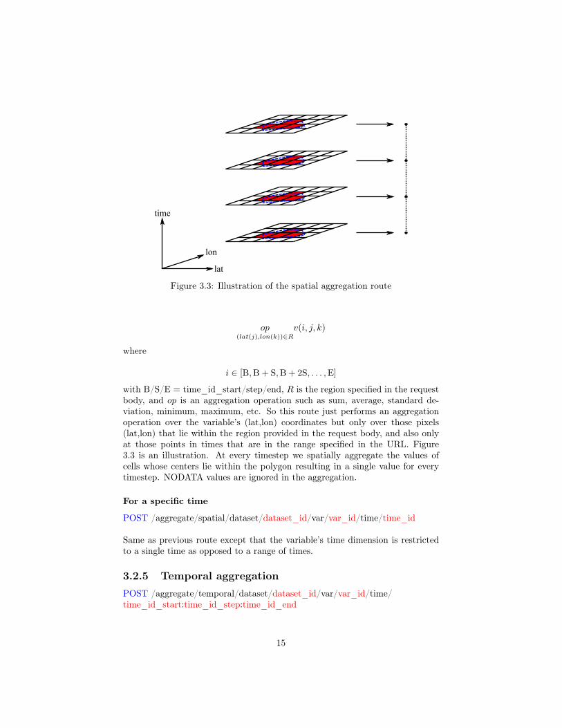
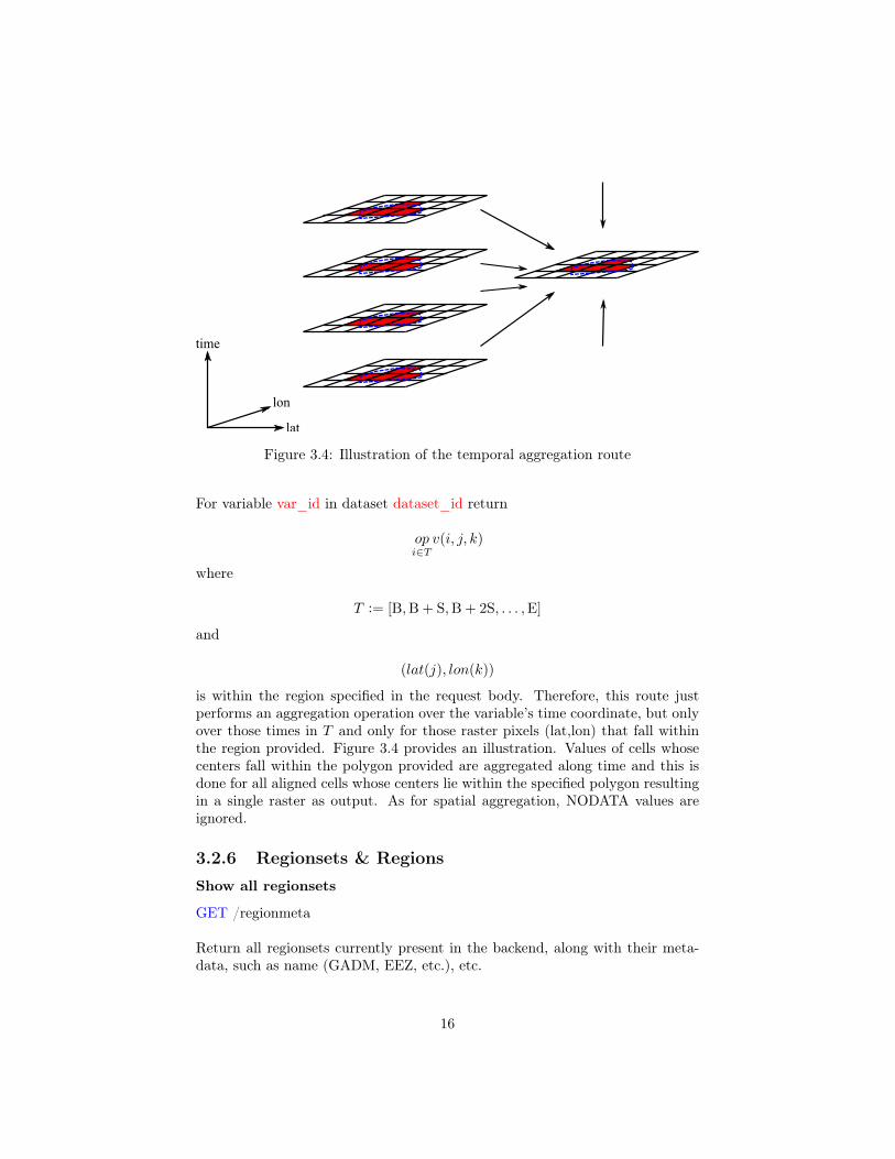
Figure 3.4: Illustration of the temporal aggregation route

For variable var_id in dataset dataset_id return

opi∈T

v(i, j, k)

where

T := [B,B+ S,B+ 2S, . . . ,E]

and

(lat(j), lon(k))

is within the region specified in the request body. Therefore, this route justperforms an aggregation operation over the variable’s time coordinate, but onlyover those times in T and only for those raster pixels (lat,lon) that fall withinthe region provided. Figure 3.4 provides an illustration. Values of cells whosecenters fall within the polygon provided are aggregated along time and this isdone for all aligned cells whose centers lie within the specified polygon resultingin a single raster as output. As for spatial aggregation, NODATA values areignored.

3.2.6 Regionsets & RegionsShow all regionsets

GET /regionmeta

Return all regionsets currently present in the backend, along with their meta-data, such as name (GADM, EEZ, etc.), etc.

16

Show a specific regionset

GET /regionmeta/regionset/regionset_id

Return a specific regionset.

Regions

POST /regiondata/regionset/regionset_id

Return all regions of a regionset that satisfy some constraints on their metadatawhere these constraints are provided in the POST request body. This route cane.g. be used to return all GADM regions for a specific level where level 0 =countries and further levels stand for finer and finer subdivisions such as states,counties, etc.

3.3 API design choicesIn this section we discuss two design choices and what the reasoning was thatled us to these choices. First, we decided to have all routes return JSON. Forsome routes however, mainly for the time range selection route, this leads toa large response resulting in overhead when transferring this response to theclient. There is also an overhead for even constructing such a large JSONwithin the EDE Flask code. Thus we could return a more compact custombinary format instead. However, this in turn requires code on the client side tounpack individual raster pixel values from such a binary format. If the clientaccesses EDE through the browser this can be solved by providing the clientwith appropriate JavaScript code that understands the custom binary format.If however the client accesses EDE from say the command line he needs todownload such code separately. Therefore, to avoid the need for extra clientsoftware we decided to have the routes return the compatible JSON formatthroughout.Second, many routes we decided to make POST routes. We started out withGET routes first and specified subsetting/aggregation regions in the URL itself.This however led to some characters being inadvertently detected as specialURL characters. Because of this and also because we realized that further downthe road more diverse request arguments would be required anyway we decidedto use a JSON body instead. This in turn required us to use an HTTP methodthat allows a body which is why we ended up with POST. In hindsight thoughGET also allows for a body and using GET instead of POST for the routes ismore in accordance with their semantics / more RESTful.

17

Chapter 4

Storing rasters in Postgres

PostgreSQL with its extension PostGIS is a natural choice for storing rasterdata since PostGIS provides a raster type. However, there is some freedom inchoosing the database schema. In particular, we can consider the timesteps inthe raster data as bands in the PostGIS raster type. However, these bands tendto be used not for timesteps but rather for different ’spectral components’ (e.g.RGB) and moreover, the maximum number of bands is hardcoded as 65536 =sizeof(uint16_t) which does support the datasets we have been working with sofar (the one with the largest number of timesteps was the AgMERRA datasetwith 11323 timesteps) though might no longer do that in the future as we adddatasets that have finer temporal resolutions (say a measurement every hour forthe last 20 years, which would mean: 20x365x24 = 175200 which would alreadyexceed the maximum number of bands). Thus it probably makes more senseto use an ’unstacked approach’ where we only store one timestep in a singlePostgres field of type raster. When using the PostGIS raster type, independentof whether we use the ’stacked’ or ’unstacked’ approach, there is another choicewe can make, namely the size of a tile. We can choose to put the entire spatialextent of a raster into a single PostGIS raster field or into multiple, each coveringa subraster/tile of some width and height that we can choose freely (impact andoptimization of this tile size would have to be studied) Lastly, one is not forcedto use the PostGIS raster type in the first place and can instead use morefundamental Postgres types such as arrays to store the time series at a fixedpixel in a raster. In this chapter we explore these different layouts of raster datawithin Postgres and determine and explain why which layout is best at meetingour expectations in terms of ingestion speed, response times, and scalability.Before we discuss the schemas and queries tried we first examine again where inthe overall architecture Postgres is embedded and rectrictions imposed becauseof that as well as give a quick description of the PostGIS extension with thetypes and functions it provides.

18

4.1 Keeping middleware overhead lowLooking again at 3.1 we see that the ”EDE Flask code” component is the one thatcommunicates directly with Postgres. It issues (as for now) raw SQL queriesand wraps Postgres’ query response into a JSON. In doing so there are multipleoverheads.First, the obvious communication overhead between the Flask code and Post-gres which can be kept low by making sure the Postgres queries return compactresponses.Second, overhead between the Flask code and Postgres also comes from iterat-ing over a Postgres response set of rows within Flask which will require multipleround-trip times between Flask and Postgres. This is in particular the case ifwe say iterate, using the Postgres client library psycopg2 for example, to obtainone raster pixel from Postgres at a time. Thus, we can minimize this number ofround-trip times by choosing queries that return only a single row by aggregat-ing the raster pixels already within Postgres into a single row. This way only asingle row will be sent from Postgres to Flask. We can go even further and makePostgres return JSON already. Say for the single time data selection route, wecan make Postgres return exactly that sub-JSON that is the value for the keydata in the overall response JSON for that route, which is actually what we doas we will see.If we do that however, a third overhead will become significant, namely, thedeserialization and serialization occurring within the Python Flask code. If wedecide to send JSON from Postgres to Flask, then Flask will deserialize thisJSON to a dictionary and after adding other response fields to that dictionary(mostly raster metadata) it will serialize it to the final response JSON. Dese-rialization is performed usually by default when using a Postgres client librarysuch as psycopg2. However, one can make sure deserialization is in fact notperformed meaning that the JSON sent by Postgres will be a string inside thePython Flask code. In order to form the final response JSON however, tediousstring concatenations would have to be performed in order to merge all thecomponents of the final response JSON.These potentials for middleware overhead influence our decision on what Post-gres shall return and thus the SQL queries and thus also the database schema.

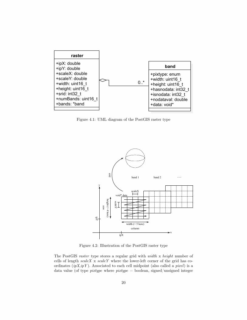
4.2 The PostGIS extensionIn this section we will briefly describe PostgreSQL’s geospatial extension Post-GIS. It provides geometry types like POINT, LINESTRING, POLYGON, andalso a raster type, along with functions to perform spatial operations on thesetypes. We will focus here on the raster type since the geometry types are ratherstraightforward. Figure 4.1 shows a simplified UML diagram of the PostGISraster and band structs appearing in the source code, we left out some structmembers like skewX, skewY. Figure 4.2 is an illustration of what these structsrepresent.

19

raster

+ipX: double+ipY: double+scaleX: double+scaleY: double+width: uint16_t+height: uint16_t+srid: int32_t+numBands: uint16_t+bands: *band

band

+pixtype: enum+width: uint16_t+height: uint16_t+hasnodata: int32_t+isnodata: int32_t+nodataval: double+data: void*

0..*

Figure 4.1: UML diagram of the PostGIS raster type

ipX

ipY

x

y

scaleX

scaleY

void* data

band 1

width (= 5 here)

height (= 4 here)

row

column

band 2 ......

srid

Figure 4.2: Illustration of the PostGIS raster type

The PostGIS raster type stores a regular grid with width x height number ofcells of length scaleX x scaleY where the lower-left corner of the grid has co-ordinates (ipX,ipY ). Associated to each cell midpoint (also called a pixel) is adata value (of type pixtype where pixtype = boolean, signed/unsigned integer

20

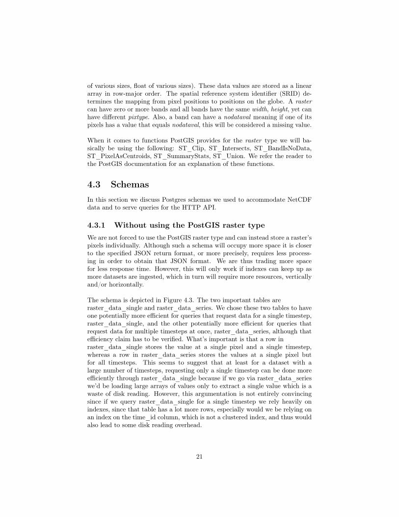
of various sizes, float of various sizes). These data values are stored as a lineararray in row-major order. The spatial reference system identifier (SRID) de-termines the mapping from pixel positions to positions on the globe. A rastercan have zero or more bands and all bands have the same width, height, yet canhave different pixtype. Also, a band can have a nodataval meaning if one of itspixels has a value that equals nodataval, this will be considered a missing value.

When it comes to functions PostGIS provides for the raster type we will ba-sically be using the following: ST_Clip, ST_Intersects, ST_BandIsNoData,ST_PixelAsCentroids, ST_SummaryStats, ST_Union. We refer the reader tothe PostGIS documentation for an explanation of these functions.

4.3 SchemasIn this section we discuss Postgres schemas we used to accommodate NetCDFdata and to serve queries for the HTTP API.

4.3.1 Without using the PostGIS raster typeWe are not forced to use the PostGIS raster type and can instead store a raster’spixels individually. Although such a schema will occupy more space it is closerto the specified JSON return format, or more precisely, requires less process-ing in order to obtain that JSON format. We are thus trading more spacefor less response time. However, this will only work if indexes can keep up asmore datasets are ingested, which in turn will require more resources, verticallyand/or horizontally.

The schema is depicted in Figure 4.3. The two important tables areraster_data_single and raster_data_series. We chose these two tables to haveone potentially more efficient for queries that request data for a single timestep,raster_data_single, and the other potentially more efficient for queries thatrequest data for multiple timesteps at once, raster_data_series, although thatefficiency claim has to be verified. What’s important is that a row inraster_data_single stores the value at a single pixel and a single timestep,whereas a row in raster_data_series stores the values at a single pixel butfor all timesteps. This seems to suggest that at least for a dataset with alarge number of timesteps, requesting only a single timestep can be done moreefficiently through raster_data_single because if we go via raster_data_serieswe’d be loading large arrays of values only to extract a single value which is awaste of disk reading. However, this argumentation is not entirely convincingsince if we query raster_data_single for a single timestep we rely heavily onindexes, since that table has a lot more rows, especially would we be relying onan index on the time_id column, which is not a clustered index, and thus wouldalso lead to some disk reading overhead.

21

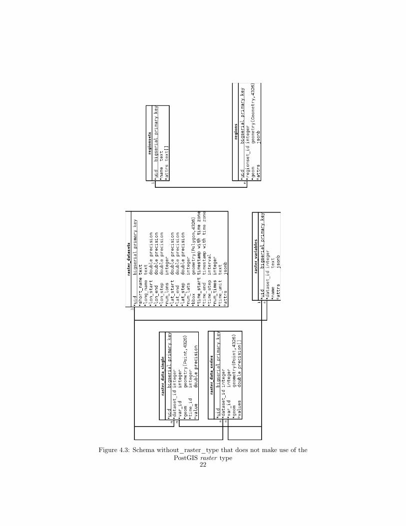
Figure 4.3: Schema without_raster_type that does not make use of thePostGIS raster type

22

4.3.2 The unstacked approachA seemingly obvious approach to storing raster data in Postgres is to use theraster type provided by the PostGIS extension. The advantage of this approachis that it is a very compact representation requiring much less space than theprevious approach. Moreover, spatial and temporal aggregation operations canbe performed more efficiently in this format. However, this comes at a price.Now that we no longer store the pixel positions of a raster individually, but onlythe values at these positions in the compact PostGIS raster type (in the void*data field, see Diagram 4.1), we require extra processing to reconstruct thesepixel positions in order to construct the response JSON, which, to emphasizeit again, needs the latitudes and longitudes of all individual pixels in the raster(see the API specification on ede_rest_api and the discussion in Section 3.2).On a very high-level therefore we are trading less space for more processing time.

Figure 4.4 shows the new schema. It is identical to Figure 4.3 except the actualdata is now stored in the raster_data table as opposed to the raster_data_singleand raster_data_series tables before. The PostGIS raster type comprises ofseveral bands, see Section 4.2. However, in this schema we store only one bandin a raster field, which holds the data for a specific time. What we do thoughis to ’tile’ an entire NetCDF raster’s extent into several PostGIS raster fields.’Tiling’ a raster just means splitting the entire raster’s extent, which is just arectangle, into subrectangles (here, these tiles don’t overlap plus are of the sameheight and width). Thus, each PostGIS ’rast’ field in this schema contains, fora fixed dataset (dataset_id), for a fixed variable within that dataset (var_id),for a fixed time (time_id) of that (time-dependent) variable, all the values, butonly within a tile of the entire spatial coverage of that variable. The size of thetiles (i.e. width & height expressed in numbers of pixels) is decided at ingestiontime though one can retile within the database later to obtain a more optimaltile size.

4.4 QueriesWe now show the Postgres queries corresponding to the HTTP routes specified inthe REST API ede_rest_api for the schema in Figure 4.3. Some routes will leadto multiple SQL queries since we not only have to get the actual raster valuesfrom the database but also the metadata associated to datasets and variables.We will refer to the routes by their names: ”Show a specific/all dataset/s”, ”Selectraster data for a specific time/time range”, ”Do spatial aggregation for a specifictime/time range”, ”Do temporal aggregation”, ”Show a specific/all regionset/s”,”List regions”, and additionally distinguish whether, for POST requests wherethe body specifies a region, the region is specified directly (i.e. by specifying itsgeometry directly which will e.g. be done when restricting the returned datato the browser’s viewport) or indirectly (i.e. a GADM or other kind of regionresiding in the database itself), even though that does not have much of an

23

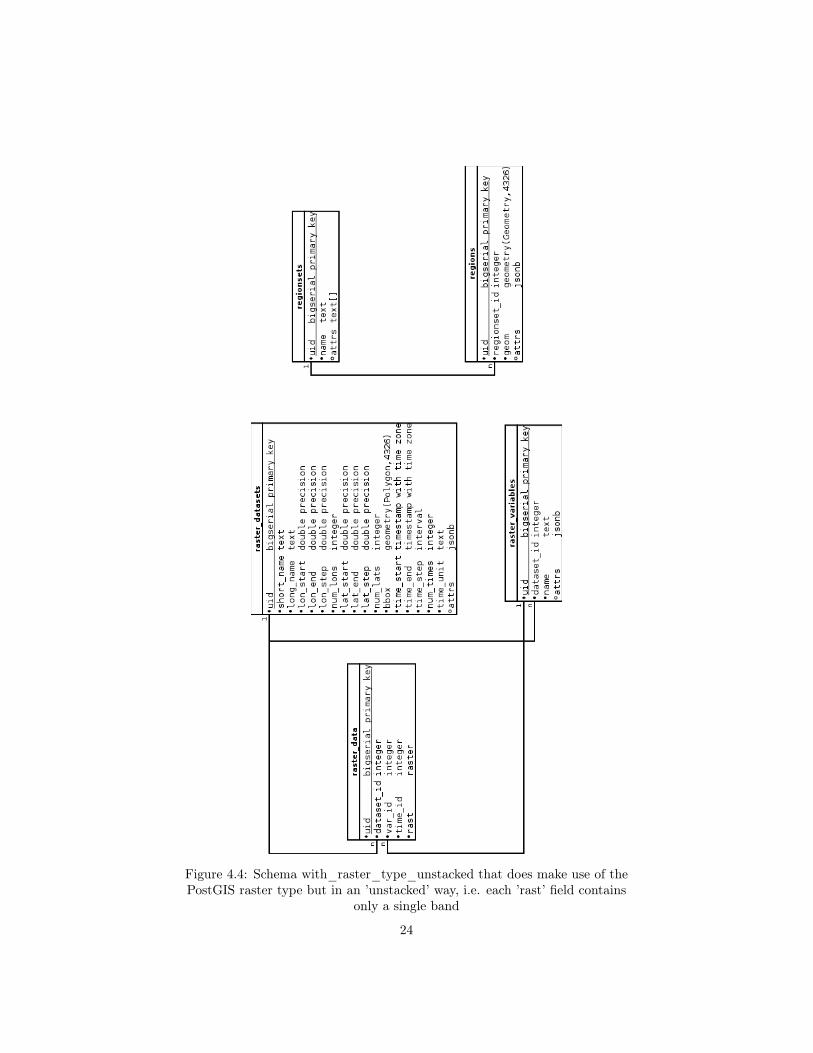
Figure 4.4: Schema with_raster_type_unstacked that does make use of thePostGIS raster type but in an ’unstacked’ way, i.e. each ’rast’ field contains

only a single band

24

impact on how the query will look, but we do it for the purpose of completeness.Last but not least we note the obvious but important, that even though nowwe have decided on a specific database schema we are still free to choose thequeries, they are not fully determined by the schema. Thus, the queries weshow here still have to be improved both in terms of speed and readability. Thebold and red-colored variables that appear in the queries are the user-providedarguments filled-in (they come from the arguments in the corresponding HTTPrequest).

4.4.1 Without the PostGIS raster typeWe here describe the queries for the schema that does not make use of thePostGIS raster type, see Section 4.3.1. The version for these queries iswithout_raster_type-v0.2.3.

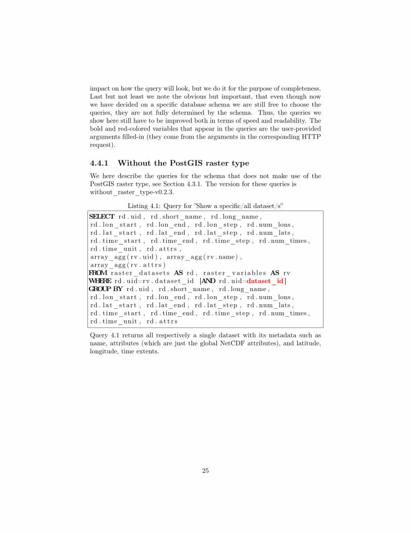
Listing 4.1: Query for ”Show a specific/all dataset/s”

SELECT rd . uid , rd . short_name , rd . long_name ,rd . lon_start , rd . lon_end , rd . lon_step , rd . num_lons ,rd . l a t_star t , rd . lat_end , rd . lat_step , rd . num_lats ,rd . t ime_start , rd . time_end , rd . time_step , rd . num_times ,rd . time_unit , rd . a t t r s ,array_agg ( rv . uid ) , array_agg ( rv . name) ,array_agg ( rv . a t t r s )FROM r a s t e r_data s e t s AS rd , r a s t e r_va r i ab l e s AS rvWHERE rd . uid=rv . dataset_id [AND rd . uid=dataset_id ]GROUPBY rd . uid , rd . short_name , rd . long_name ,rd . lon_start , rd . lon_end , rd . lon_step , rd . num_lons ,rd . l a t_star t , rd . lat_end , rd . lat_step , rd . num_lats ,rd . t ime_start , rd . time_end , rd . time_step , rd . num_times ,rd . time_unit , rd . a t t r s

Query 4.1 returns all respectively a single dataset with its metadata such asname, attributes (which are just the global NetCDF attributes), and latitude,longitude, time extents.

25

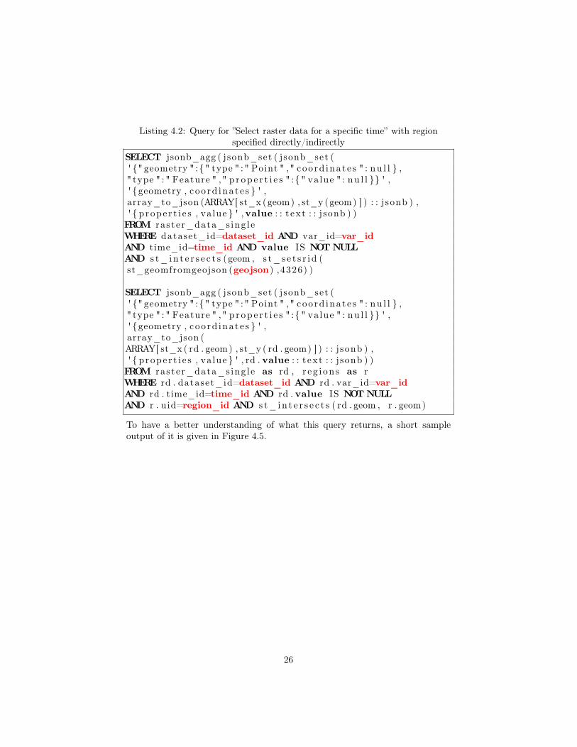
Listing 4.2: Query for ”Select raster data for a specific time” with regionspecified directly/indirectly

SELECT jsonb_agg ( jsonb_set ( jsonb_set (' {" geometry " :{" type " :" Point " ," coo rd ina t e s " : nu l l } ," type " :" Feature " ," p r op e r t i e s " :{" value " : nu l l }} ' ,' {geometry , c oo rd ina t e s } ' ,array_to_json (ARRAY[ st_x (geom) , st_y (geom) ] ) : : j sonb ) ,' { p rope r t i e s , va lue } ' ,value : : t ex t : : j sonb ) )FROM ras te r_data_s ing leWHERE dataset_id=dataset_id AND var_id=var_idAND time_id=time_id AND value IS NOTNULLAND s t_ i n t e r s e c t s (geom , s t_s e t s r i d (st_geomfromgeojson (geojson) ,4326) )

SELECT jsonb_agg ( jsonb_set ( jsonb_set (' {" geometry " :{" type " :" Point " ," coo rd ina t e s " : nu l l } ," type " :" Feature " ," p r op e r t i e s " :{" value " : nu l l }} ' ,' {geometry , c oo rd ina t e s } ' ,array_to_json (ARRAY[ st_x ( rd . geom) , st_y ( rd . geom) ] ) : : j sonb ) ,' { p rope r t i e s , va lue } ' , rd . value : : t ex t : : j sonb ) )FROM ras te r_data_s ing le as rd , r e g i on s as rWHERE rd . dataset_id=dataset_id AND rd . var_id=var_idAND rd . time_id=time_id AND rd . value IS NOTNULLAND r . uid=region_id AND s t_ i n t e r s e c t s ( rd . geom , r . geom)

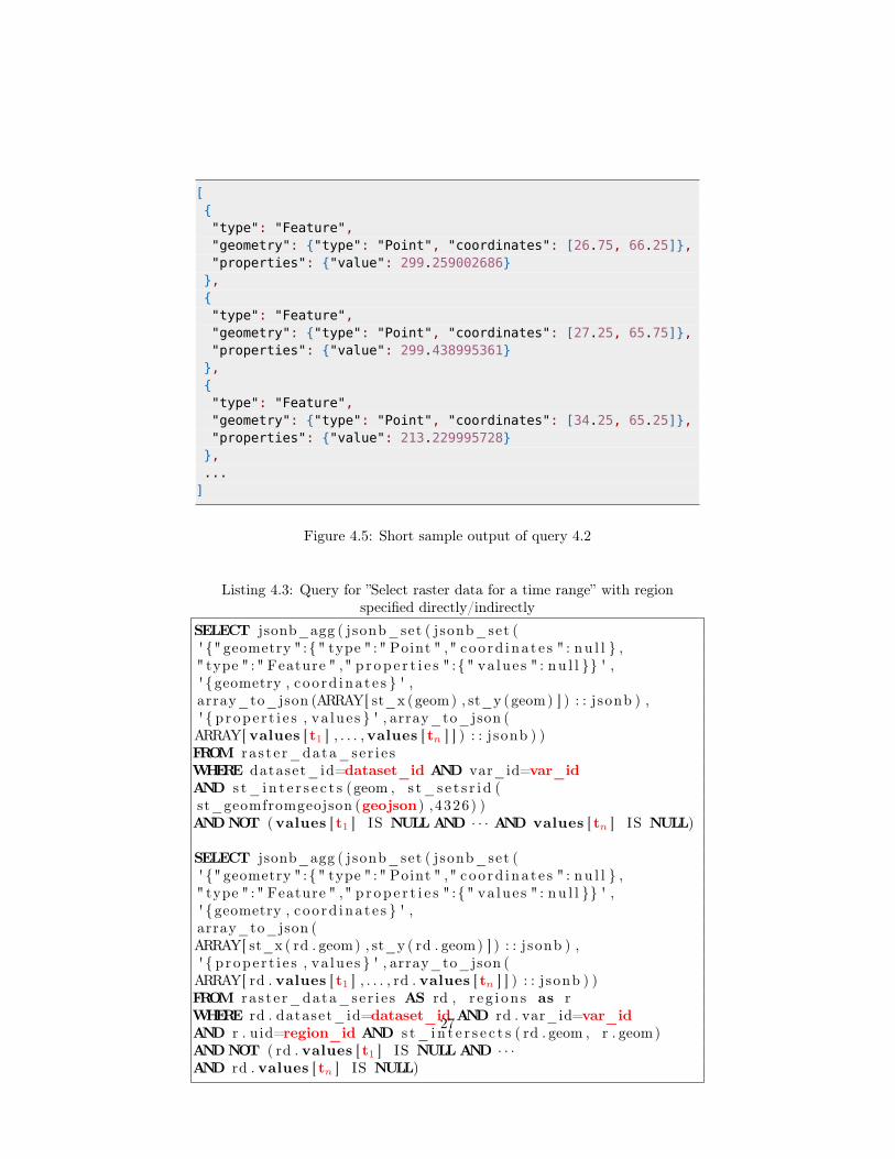
To have a better understanding of what this query returns, a short sampleoutput of it is given in Figure 4.5.

26

[{"type": "Feature","geometry": {"type": "Point", "coordinates": [26.75, 66.25]},"properties": {"value": 299.259002686}},{"type": "Feature","geometry": {"type": "Point", "coordinates": [27.25, 65.75]},"properties": {"value": 299.438995361}},{"type": "Feature","geometry": {"type": "Point", "coordinates": [34.25, 65.25]},"properties": {"value": 213.229995728}},...]

Figure 4.5: Short sample output of query 4.2

Listing 4.3: Query for ”Select raster data for a time range” with regionspecified directly/indirectly

SELECT jsonb_agg ( jsonb_set ( jsonb_set (' {" geometry " :{" type " :" Point " ," coo rd ina t e s " : nu l l } ," type " :" Feature " ," p r op e r t i e s " :{" va lue s " : nu l l }} ' ,' {geometry , c oo rd ina t e s } ' ,array_to_json (ARRAY[ st_x (geom) , st_y (geom) ] ) : : j sonb ) ,' { p rope r t i e s , va lue s } ' , array_to_json (ARRAY[ values [ t1 ] , . . . ,values [ tn ] ] ) : : j sonb ) )FROM ra s t e r_data_ser i e sWHERE dataset_id=dataset_id AND var_id=var_idAND s t_ i n t e r s e c t s (geom , s t_s e t s r i d (st_geomfromgeojson (geojson) ,4326) )ANDNOT (values [ t1 ] IS NULLAND · · · AND values [ tn ] IS NULL)

SELECT jsonb_agg ( jsonb_set ( jsonb_set (' {" geometry " :{" type " :" Point " ," coo rd ina t e s " : nu l l } ," type " :" Feature " ," p r op e r t i e s " :{" va lue s " : nu l l }} ' ,' {geometry , c oo rd ina t e s } ' ,array_to_json (ARRAY[ st_x ( rd . geom) , st_y ( rd . geom) ] ) : : j sonb ) ,' { p rope r t i e s , va lue s } ' , array_to_json (ARRAY[ rd . values [ t1 ] , . . . , rd . values [ tn ] ] ) : : j sonb ) )FROM ra s t e r_data_ser i e s AS rd , r e g i on s as rWHERE rd . dataset_id=dataset_id AND rd . var_id=var_idAND r . uid=region_id AND s t_ i n t e r s e c t s ( rd . geom , r . geom)ANDNOT ( rd . values [ t1 ] IS NULLAND · · ·AND rd . values [ tn ] IS NULL)

27

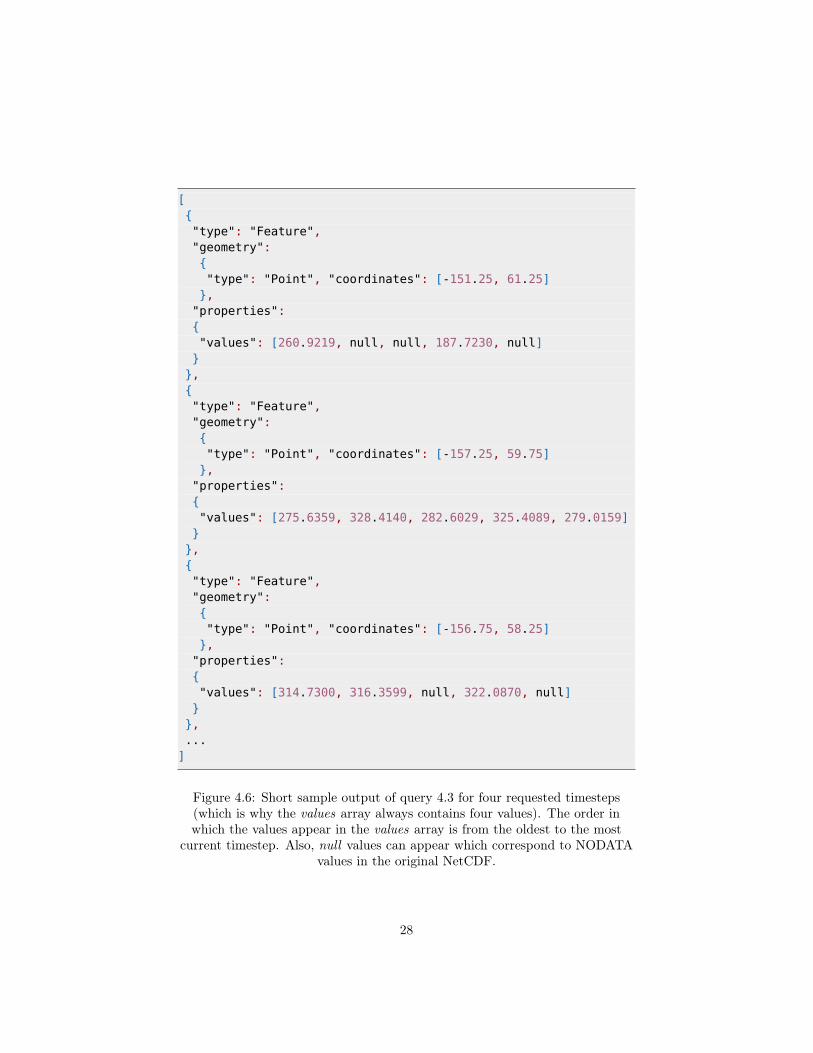
[{"type": "Feature","geometry":{"type": "Point", "coordinates": [-151.25, 61.25]},"properties":{"values": [260.9219, null, null, 187.7230, null]}},{"type": "Feature","geometry":{"type": "Point", "coordinates": [-157.25, 59.75]},"properties":{"values": [275.6359, 328.4140, 282.6029, 325.4089, 279.0159]}},{"type": "Feature","geometry":{"type": "Point", "coordinates": [-156.75, 58.25]},"properties":{"values": [314.7300, 316.3599, null, 322.0870, null]}},...]

Figure 4.6: Short sample output of query 4.3 for four requested timesteps(which is why the values array always contains four values). The order inwhich the values appear in the values array is from the oldest to the most

current timestep. Also, null values can appear which correspond to NODATAvalues in the original NetCDF.

28

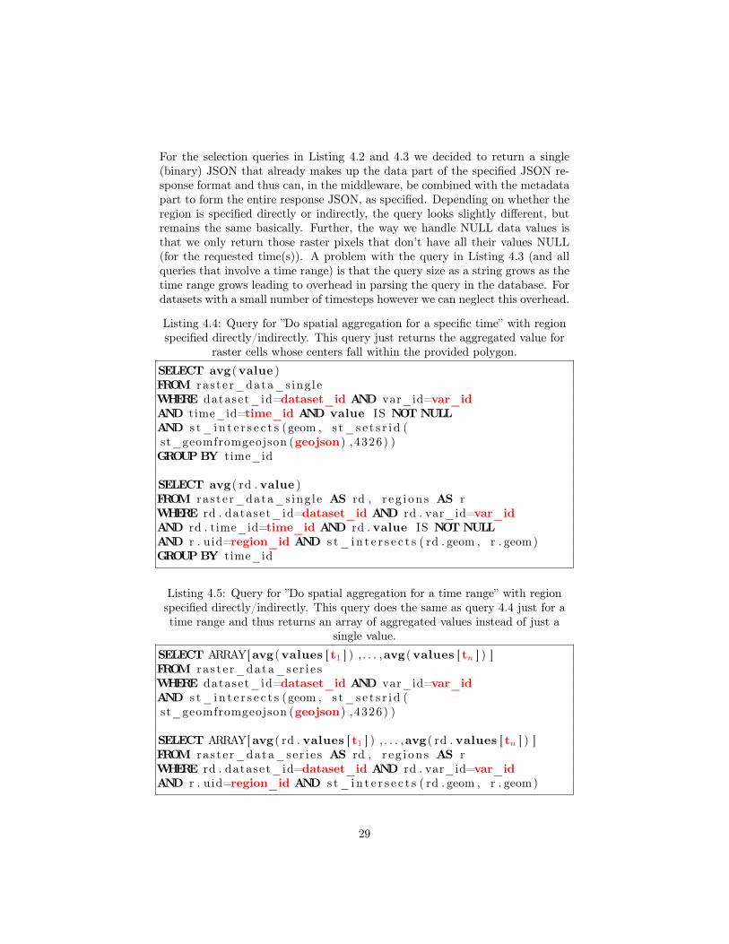
For the selection queries in Listing 4.2 and 4.3 we decided to return a single(binary) JSON that already makes up the data part of the specified JSON re-sponse format and thus can, in the middleware, be combined with the metadatapart to form the entire response JSON, as specified. Depending on whether theregion is specified directly or indirectly, the query looks slightly different, butremains the same basically. Further, the way we handle NULL data values isthat we only return those raster pixels that don’t have all their values NULL(for the requested time(s)). A problem with the query in Listing 4.3 (and allqueries that involve a time range) is that the query size as a string grows as thetime range grows leading to overhead in parsing the query in the database. Fordatasets with a small number of timesteps however we can neglect this overhead.

Listing 4.4: Query for ”Do spatial aggregation for a specific time” with regionspecified directly/indirectly. This query just returns the aggregated value for

raster cells whose centers fall within the provided polygon.

SELECT avg (value )FROM ras te r_data_s ing leWHERE dataset_id=dataset_id AND var_id=var_idAND time_id=time_id AND value IS NOTNULLAND s t_ i n t e r s e c t s (geom , s t_s e t s r i d (st_geomfromgeojson (geojson) ,4326) )GROUPBY time_id

SELECT avg ( rd . value )FROM ras te r_data_s ing le AS rd , r e g i on s AS rWHERE rd . dataset_id=dataset_id AND rd . var_id=var_idAND rd . time_id=time_id AND rd . value IS NOTNULLAND r . uid=region_id AND s t_ i n t e r s e c t s ( rd . geom , r . geom)GROUPBY time_id

Listing 4.5: Query for ”Do spatial aggregation for a time range” with regionspecified directly/indirectly. This query does the same as query 4.4 just for atime range and thus returns an array of aggregated values instead of just a

single value.

SELECT ARRAY[ avg (values [ t1 ] ) , . . . ,avg (values [ tn ] ) ]FROM ra s t e r_data_ser i e sWHERE dataset_id=dataset_id AND var_id=var_idAND s t_ i n t e r s e c t s (geom , s t_s e t s r i d (st_geomfromgeojson (geojson) ,4326) )

SELECT ARRAY[ avg ( rd . values [ t1 ] ) , . . . ,avg ( rd . values [ tn ] ) ]FROM ra s t e r_data_ser i e s AS rd , r e g i on s AS rWHERE rd . dataset_id=dataset_id AND rd . var_id=var_idAND r . uid=region_id AND s t_ i n t e r s e c t s ( rd . geom , r . geom)

29

When it comes to spatial aggregation we have so far hardcoded the aggregationoperation to be the average. However, other operations such as sum, min, max,stddev can be used just in place of avg. For benchmarking purposes this won’tmatter as independent of the operation, the aggregation is a one-time pass (evenfor stddev).

30

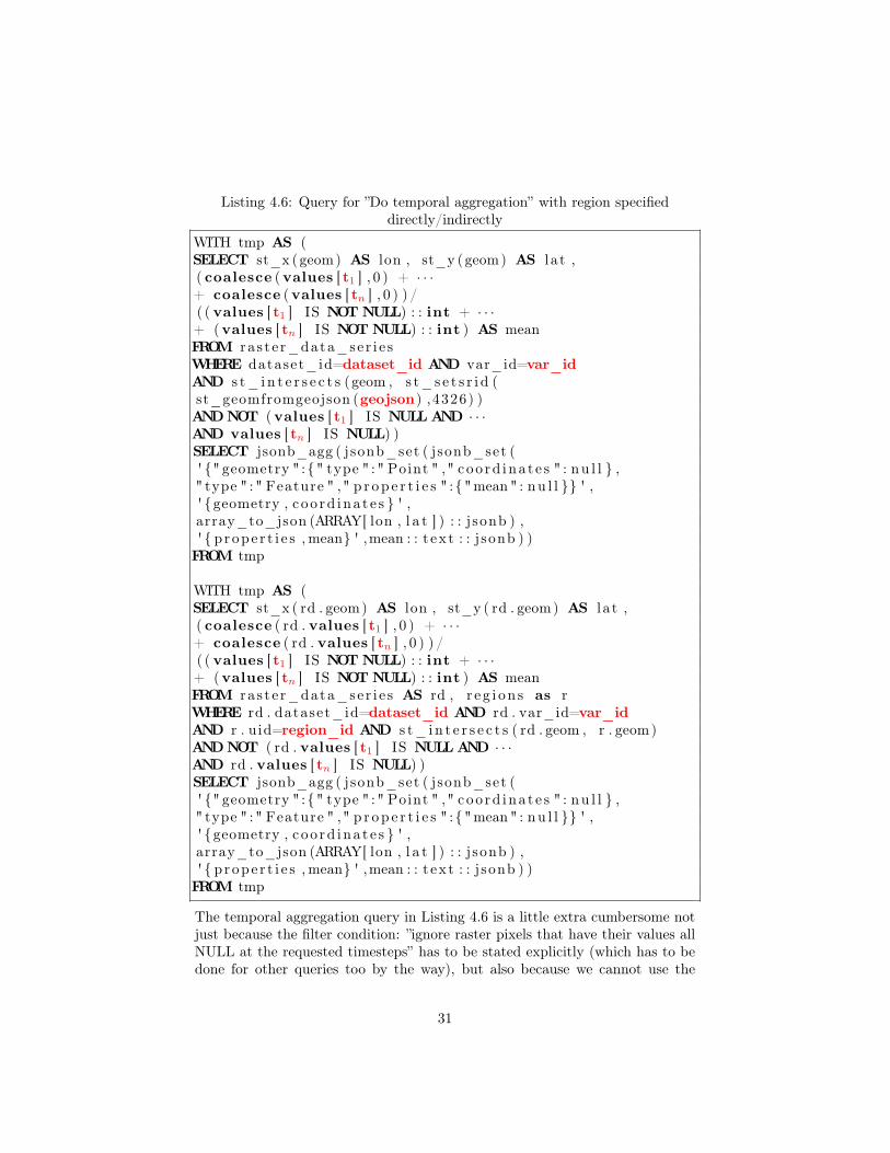
Listing 4.6: Query for ”Do temporal aggregation” with region specifieddirectly/indirectly

WITH tmp AS (SELECT st_x (geom) AS lon , st_y (geom) AS l a t ,( coalesce (values [ t1 ] , 0 ) + · · ·+ coalesce (values [ tn ] , 0 ) ) /( ( values [ t1 ] IS NOTNULL) : : int + · · ·+ (values [ tn ] IS NOTNULL) : : int ) AS meanFROM ra s t e r_data_ser i e sWHERE dataset_id=dataset_id AND var_id=var_idAND s t_ i n t e r s e c t s (geom , s t_s e t s r i d (st_geomfromgeojson (geojson) ,4326) )ANDNOT (values [ t1 ] IS NULLAND · · ·AND values [ tn ] IS NULL) )SELECT jsonb_agg ( jsonb_set ( jsonb_set (' {" geometry " :{" type " :" Point " ," coo rd ina t e s " : nu l l } ," type " :" Feature " ," p r op e r t i e s " :{"mean" : nu l l }} ' ,' {geometry , c oo rd ina t e s } ' ,array_to_json (ARRAY[ lon , l a t ] ) : : j sonb ) ,' { p rope r t i e s ,mean} ' ,mean : : t ex t : : j sonb ) )FROM tmp

WITH tmp AS (SELECT st_x ( rd . geom) AS lon , st_y ( rd . geom) AS l a t ,( coalesce ( rd . values [ t1 ] , 0 ) + · · ·+ coalesce ( rd . values [ tn ] , 0 ) ) /( ( values [ t1 ] IS NOTNULL) : : int + · · ·+ (values [ tn ] IS NOTNULL) : : int ) AS meanFROM ra s t e r_data_ser i e s AS rd , r e g i on s as rWHERE rd . dataset_id=dataset_id AND rd . var_id=var_idAND r . uid=region_id AND s t_ i n t e r s e c t s ( rd . geom , r . geom)ANDNOT ( rd . values [ t1 ] IS NULLAND · · ·AND rd . values [ tn ] IS NULL) )SELECT jsonb_agg ( jsonb_set ( jsonb_set (' {" geometry " :{" type " :" Point " ," coo rd ina t e s " : nu l l } ," type " :" Feature " ," p r op e r t i e s " :{"mean" : nu l l }} ' ,' {geometry , c oo rd ina t e s } ' ,array_to_json (ARRAY[ lon , l a t ] ) : : j sonb ) ,' { p rope r t i e s ,mean} ' ,mean : : t ex t : : j sonb ) )FROM tmp

The temporal aggregation query in Listing 4.6 is a little extra cumbersome notjust because the filter condition: ”ignore raster pixels that have their values allNULL at the requested timesteps” has to be stated explicitly (which has to bedone for other queries too by the way), but also because we cannot use the

31

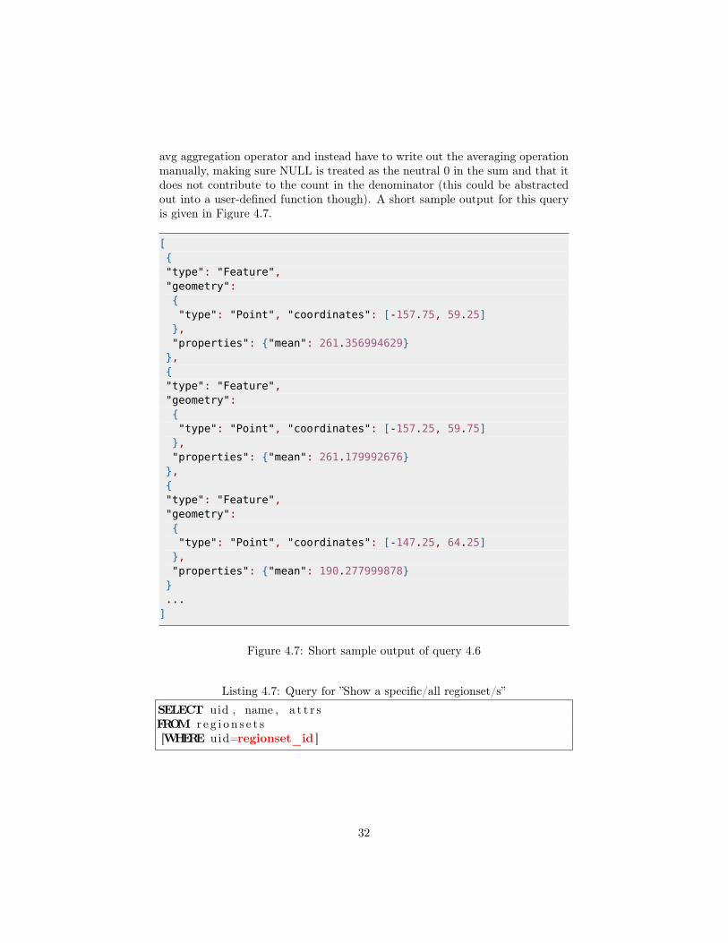
avg aggregation operator and instead have to write out the averaging operationmanually, making sure NULL is treated as the neutral 0 in the sum and that itdoes not contribute to the count in the denominator (this could be abstractedout into a user-defined function though). A short sample output for this queryis given in Figure 4.7.

[{"type": "Feature","geometry":{"type": "Point", "coordinates": [-157.75, 59.25]},"properties": {"mean": 261.356994629}},{"type": "Feature","geometry":{"type": "Point", "coordinates": [-157.25, 59.75]},"properties": {"mean": 261.179992676}},{"type": "Feature","geometry":{"type": "Point", "coordinates": [-147.25, 64.25]},"properties": {"mean": 190.277999878}}...]

Figure 4.7: Short sample output of query 4.6

Listing 4.7: Query for ”Show a specific/all regionset/s”

SELECT uid , name , a t t r sFROM r e g i o n s e t s[WHERE uid=regionset_id ]

32

Listing 4.8: Query for ”List regions”

SELECT uid , s t_asgeo j son (geom)FROM r e g i on sWHERE r eg ionse t_id=regionset_id[AND a t t r s ->>name1=value1 AND · · · AND a t t r s ->>namem=valuem ]

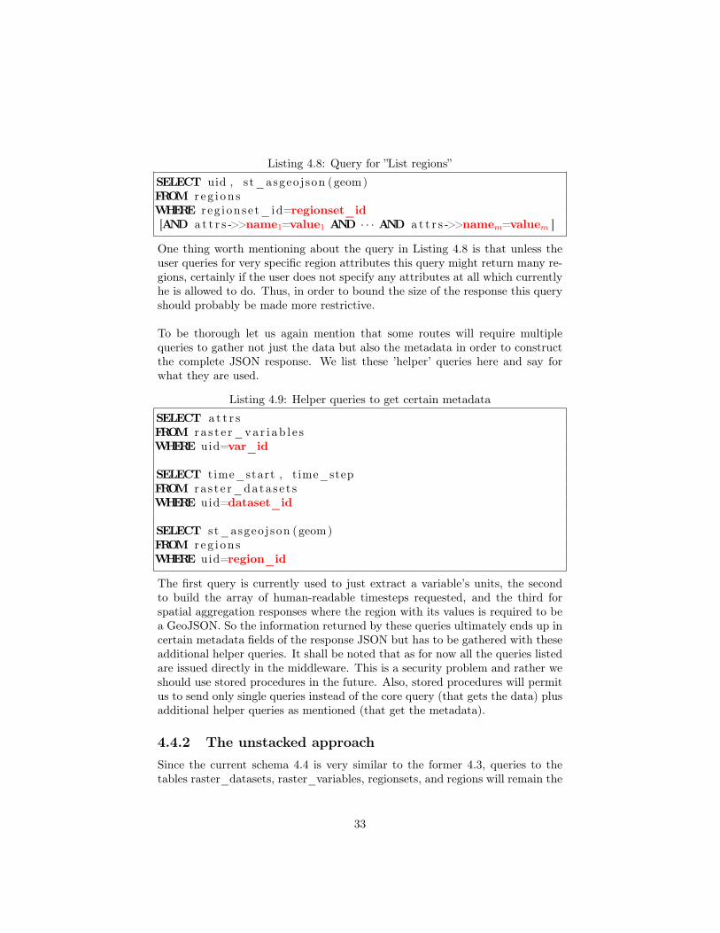
One thing worth mentioning about the query in Listing 4.8 is that unless theuser queries for very specific region attributes this query might return many re-gions, certainly if the user does not specify any attributes at all which currentlyhe is allowed to do. Thus, in order to bound the size of the response this queryshould probably be made more restrictive.

To be thorough let us again mention that some routes will require multiplequeries to gather not just the data but also the metadata in order to constructthe complete JSON response. We list these ’helper’ queries here and say forwhat they are used.

Listing 4.9: Helper queries to get certain metadata

SELECT a t t r sFROM r a s t e r_va r i ab l e sWHERE uid=var_id

SELECT t ime_start , time_stepFROM r a s t e r_data s e t sWHERE uid=dataset_id

SELECT s t_asgeoj son (geom)FROM r e g i on sWHERE uid=region_id

The first query is currently used to just extract a variable’s units, the secondto build the array of human-readable timesteps requested, and the third forspatial aggregation responses where the region with its values is required to bea GeoJSON. So the information returned by these queries ultimately ends up incertain metadata fields of the response JSON but has to be gathered with theseadditional helper queries. It shall be noted that as for now all the queries listedare issued directly in the middleware. This is a security problem and rather weshould use stored procedures in the future. Also, stored procedures will permitus to send only single queries instead of the core query (that gets the data) plusadditional helper queries as mentioned (that get the metadata).

4.4.2 The unstacked approachSince the current schema 4.4 is very similar to the former 4.3, queries to thetables raster_datasets, raster_variables, regionsets, and regions will remain the

33

same (in particular also the mentioned helper queries required to get metadatato construct the complete response JSON consisting of data and metadata).Queries to these tables are not critical anyway for testing the efficiency andscalability of the proposed schemas because these tables are small (e.g. theraster_datasets table only has one row per dataset and the regions table willmostly contain GADM regions which don’t change, basically). Further, wehave decided to make the queries return the same as the queries for the pre-vious schema. Thus, the selection and temporal aggregation queries return aJSON which is then inserted, in the middleware, into the entire response JSON,together with metadata obtained from other tables through helper queries. Be-cause these queries return these JSONs they need to unpack the pixels withinthe PostGIS raster type, through the function ST_PixelAsCentroids. It is thisunpacking that is responsible for some considerably large query response timesas we shall see soon. Of course these queries don’t have to return JSON but in-stead could return the more compact PostGIS raster type which would be fasterto send to the middleware anyway, and of course also from there to the user’sbrowser. However, the unpacking of the individual pixels from that PostGISraster type would then have to be performed within the user’s browser process,i.e. through JavaScript and say typed arrays and data views. It remains to beseen whether this approach is faster overall and suitable so we defer consideringit for now. Thus, as mentioned, the queries return the same JSONs as in theprevious schema and we list these queries in this section. For the sake of brevitywe will only show the selection and aggregation queries in the case where theregion is provided directly, i.e. as a GeoJSON, and not also the version wherethe region is provided indirectly, i.e. as an identifier of a GADM region presentin the database. That’s because these two cases were already written out veryverbosely for the previous schema and are very similar anyway. The queries de-scribed here correspond to EDE version with_raster_type_unstacked-v0.2.1.

34

Listing 4.10: Query for ”Select raster data for a specific time” with regionspecified directly

WITH tmp1 AS(SELECT s t_c l i p ( rast , s t_s e t s r i d ( st_geomfromgeojson (

geojson) ,4326) , true ) AS r a s tFROM raster_dataWHERE dataset_id=dataset_id AND var_id=var_idAND time_id=time_id AND s t_ i n t e r s e c t s ( rast , s t_s e t s r i d (

st_geomfromgeojson (geojson) ,4326) )ANDNOT st_bandisnodata ( r a s t ) ) ,tmp2 AS(SELECT ( s t_p i x e l a s c en t r o i d s ( r a s t ) ) .∗FROM tmp1)SELECT jsonb_agg ( jsonb_set ( jsonb_set (' {" geometry " :{" type " :" Point " ," coo rd ina t e s " : nu l l } ," type " :" Feature " ," p r op e r t i e s " :{" value " : nu l l }} ' ,' {geometry , c oo rd ina t e s } ' ,array_to_json (ARRAY[ st_x (geom) , st_y (geom) ] ) : : j sonb ) ,' { p rope r t i e s , va lue } ' , va l : : t ex t : : j sonb ) )FROM tmp2

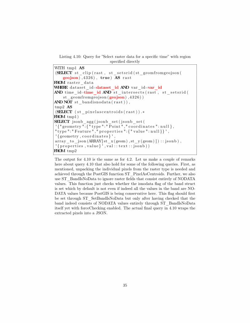
The output for 4.10 is the same as for 4.2. Let us make a couple of remarkshere about query 4.10 that also hold for some of the following queries. First, asmentioned, unpacking the individual pixels from the raster type is needed andachieved through the PostGIS function ST_PixelAsCentroids. Further, we alsouse ST_BandIsNoData to ignore raster fields that consist entirely of NODATAvalues. This function just checks whether the isnodata flag of the band structis set which by default is not even if indeed all the values in the band are NO-DATA values because PostGIS is being conservative here. This flag should firstbe set through ST_SetBandIsNoData but only after having checked that theband indeed consists of NODATA values entirely through ST_BandIsNoDataitself yet with forceChecking enabled. The actual final query in 4.10 wraps theextracted pixels into a JSON.

35

Listing 4.11: Query for ”Select raster data for a time range” with regionspecified directly

WITH tmp1 AS(SELECT time_id , s t_c l i p ( rast , s t_s e t s r i d (

st_geomfromgeojson (geojson) ,4326) , true ) AS r a s tFROM raster_dataWHERE dataset_id=dataset_id AND var_id=var_idAND time_id IN (t1,...,tn) AND s t_ i n t e r s e c t s ( rast , s t_s e t s r i d

( st_geomfromgeojson (geojson) ,4326) )ANDNOT st_bandisnodata ( r a s t ) ) ,tmp2 AS(SELECT time_id , ( s t_p i x e l a s c en t r o i d s ( r a s t ) ) .∗FROM tmp1) ,tmp3 AS(SELECT st_x (geom) AS lon , st_y (geom) AS l a t ,

f i l l_up_with_nul l s ( array_agg (( time_id , va l ) : : int_double_tuple ) ,time_id_start , time_id_step , time_id_end) AS valuesFROM tmp2GROUPBY geom)SELECT jsonb_agg ( jsonb_set ( jsonb_set (' {" geometry " :{" type " :" Point " ," coo rd ina t e s " : nu l l } ," type " :" Feature " ," p r op e r t i e s "{" va lue s " : nu l l }} ' ,' {geometry , c oo rd ina t e s } ' ,array_to_json (ARRAY[ lon , l a t ] ) : : j sonb ) ,' { p rope r t i e s , va lue s } ' , array_to_json (values ) : : j sonb ) )FROM tmp3

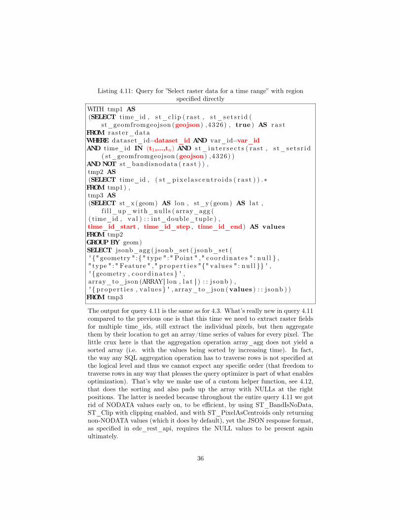
The output for query 4.11 is the same as for 4.3. What’s really new in query 4.11compared to the previous one is that this time we need to extract raster fieldsfor multiple time_ids, still extract the individual pixels, but then aggregatethem by their location to get an array/time series of values for every pixel. Thelittle crux here is that the aggregation operation array_agg does not yield asorted array (i.e. with the values being sorted by increasing time). In fact,the way any SQL aggregation operation has to traverse rows is not specified atthe logical level and thus we cannot expect any specific order (that freedom totraverse rows in any way that pleases the query optimizer is part of what enablesoptimization). That’s why we make use of a custom helper function, see 4.12,that does the sorting and also pads up the array with NULLs at the rightpositions. The latter is needed because throughout the entire query 4.11 we gotrid of NODATA values early on, to be efficient, by using ST_BandIsNoData,ST_Clip with clipping enabled, and with ST_PixelAsCentroids only returningnon-NODATA values (which it does by default), yet the JSON response format,as specified in ede_rest_api, requires the NULL values to be present againultimately.

36

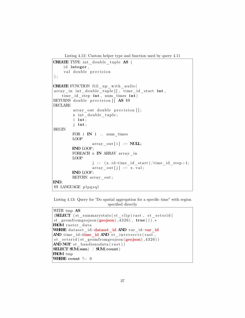
Listing 4.12: Custom helper type and function used by query 4.11

CREATE TYPE int_double_tuple AS (id integer ,va l double p r e c i s i o n

) ;

CREATE FUNCTION fi l l_up_with_nul l s (array_in int_double_tuple [ ] , t ime_id_start int ,

time_id_step int , num_times int )RETURNS double p r e c i s i o n [ ] AS $$DECLARE

array_out double p r e c i s i o n [ ] ;x int_double_tuple ;i int ;j int ;

BEGINFOR i IN 1 . . num_timesLOOP

array_out [ i ] := NULL;END LOOP;FOREACH x IN ARRAY array_inLOOP

j := (x . id -t ime_id_start ) / time_id_step+1;array_out [ j ] := x . va l ;

END LOOP;RETURN array_out ;

END;$$ LANGUAGE p lpg sq l

Listing 4.13: Query for ”Do spatial aggregation for a specific time” with regionspecified directly

WITH tmp AS(SELECT ( st_summarystats ( s t_c l i p ( rast , s t_s e t s r i d (st_geomfromgeojson (geojson) ,4326) , true ) ) ) .∗FROM raster_dataWHERE dataset_id=dataset_id AND var_id=var_idAND time_id=time_id AND s t_ i n t e r s e c t s ( rast ,s t_s e t s r i d ( st_geomfromgeojson (geojson) ,4326) )ANDNOT st_bandisnodata ( r a s t ) )SELECT SUM(sum) / SUM(count )FROM tmpWHERE count != 0

37

Listing 4.14: Query for ”Do spatial aggregation for a time range” with regionspecified directly

WITH tmp AS(SELECT time_id , ( st_summarystats ( s t_c l i p ( rast ,

s t_s e t s r i d (st_geomfromgeojson (geojson) ,4326) , true ) ) ) .∗FROM raster_dataWHERE dataset_id=dataset_id AND var_id=var_idAND time_id IN (t1,...,tn) AND s t_ i n t e r s e c t s ( rast ,s t_s e t s r i d ( st_geomfromgeojson (geojson) ,4326) )ANDNOT st_bandisnodata ( r a s t ) )SELECT SUM(sum) / SUM(count )FROM tmpWHERE count != 0GROUPBY time_idORDERBY time_id

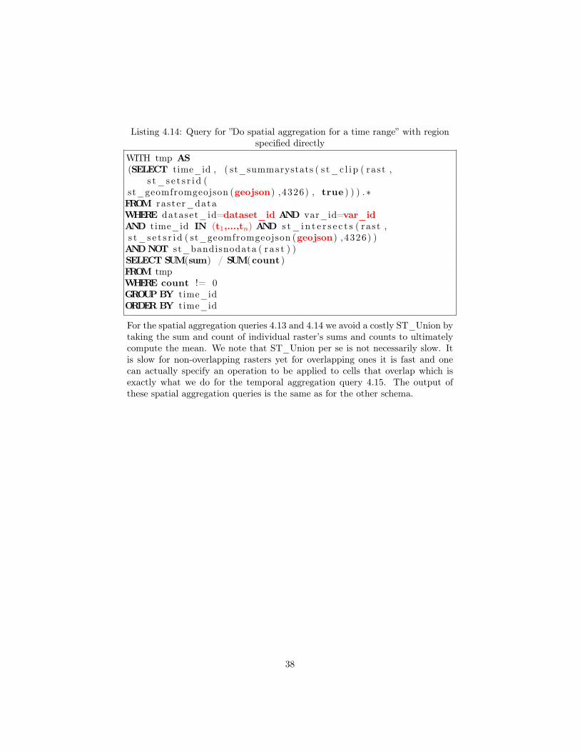
For the spatial aggregation queries 4.13 and 4.14 we avoid a costly ST_Union bytaking the sum and count of individual raster’s sums and counts to ultimatelycompute the mean. We note that ST_Union per se is not necessarily slow. Itis slow for non-overlapping rasters yet for overlapping ones it is fast and onecan actually specify an operation to be applied to cells that overlap which isexactly what we do for the temporal aggregation query 4.15. The output ofthese spatial aggregation queries is the same as for the other schema.

38

Listing 4.15: Query for ”Do temporal aggregation” with region specifieddirectly

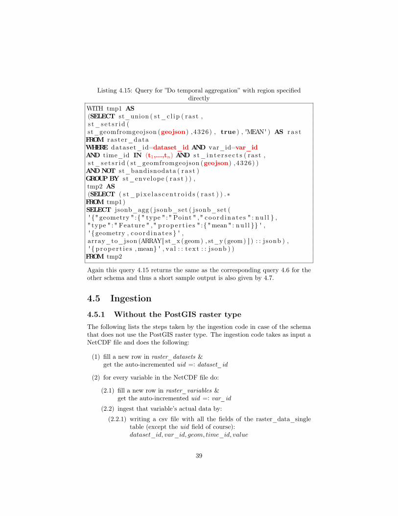
WITH tmp1 AS(SELECT st_union ( s t_c l i p ( rast ,s t_s e t s r i d (st_geomfromgeojson (geojson) ,4326) , true ) , 'MEAN' ) AS r a s tFROM raster_dataWHERE dataset_id=dataset_id AND var_id=var_idAND time_id IN (t1,...,tn) AND s t_ i n t e r s e c t s ( rast ,s t_s e t s r i d ( st_geomfromgeojson (geojson) ,4326) )ANDNOT st_bandisnodata ( r a s t )GROUPBY st_envelope ( r a s t ) ) ,tmp2 AS(SELECT ( s t_p i x e l a s c en t r o i d s ( r a s t ) ) .∗FROM tmp1)SELECT jsonb_agg ( jsonb_set ( jsonb_set (' {" geometry " :{" type " :" Point " ," coo rd ina t e s " : nu l l } ," type " :" Feature " ," p r op e r t i e s " :{"mean" : nu l l }} ' ,' {geometry , c oo rd ina t e s } ' ,array_to_json (ARRAY[ st_x (geom) , st_y (geom) ] ) : : j sonb ) ,' { p rope r t i e s ,mean} ' , va l : : t ex t : : j sonb ) )FROM tmp2

Again this query 4.15 returns the same as the corresponding query 4.6 for theother schema and thus a short sample output is also given by 4.7.

4.5 Ingestion

4.5.1 Without the PostGIS raster typeThe following lists the steps taken by the ingestion code in case of the schemathat does not use the PostGIS raster type. The ingestion code takes as input aNetCDF file and does the following:

(1) fill a new row in raster_datasets &get the auto-incremented uid =: dataset_id

(2) for every variable in the NetCDF file do:

(2.1) fill a new row in raster_variables &get the auto-incremented uid =: var_id

(2.2) ingest that variable’s actual data by:

(2.2.1) writing a csv file with all the fields of the raster_data_singletable (except the uid field of course):dataset_id, var_id, geom, time_id, value

39

(2.2.2) run Postgres’ COPY-FROM on that file to finally ingest it intothe raster_data_single table

Once the data is in raster_data_single it is carried over, via a SQL query,to the other table raster_data_series. We note that this ingestion proce-dure is wrapped into a transaction to prevent partial ingestions, e.g. end-ing up with data ingested into raster_datasets and raster_variables but notyet into raster_data_single because of a failure in between. We also notethat for every new NetCDF file, even if it belongs to the same dataset (e.g.pSIMS, AgMERRA, etc.), this ingestion procedure will create a new row inraster_datasets, which is wrong, and if the new NetCDF file has a variable thatoccurred in a previous NetCDF file, this ingestion procedure will also create anew row for that variable in raster_variables, which is also wrong, i.e. it is notsmart enough to detect that a variable’s data might be spread over multipleNetCDF files as is the case for e.g. the AgMERRA dataset. This problem ofhandling multi-file NetCDF datasets has already been mentioned in NcML andNetCDF-Java.

4.5.2 With the PostGIS raster type, unstackedFor the schema that does make use of the PostGIS raster type in an unstackedway the ingestion procedure is quite similar. Given a NetCDF file, the stepsare:

(1) fill a new row in raster_datasets &get the auto-incremented uid =: dataset_id

(2) for every variable in the NetCDF file do:

(2.1) fill a new row in raster_variables &get the auto-incremented uid =: var_id

(2.2) ingest that variable’s actual data by:looping over every tile (of a pre-configured width and height) and do:

(2.2.1) create a raster object that contains one band which itself containsthe tile

(2.2.2) serialize that raster to hexwkb, call that serialized bytesequence=: rast

(2.2.3) write a csv file with all the fields of the raster_data table (exceptthe uid field of course):dataset_id, var_id, time_id, rast

(2.2.4) run Postgres’ COPY-FROM on that file to finally ingest it intothe raster_data table

As before for the other schema this ingestion procedure also does not properlyhandle multi-file NetCDF datasets and this would have to be solved with whatis described in Section 2.2.

40

4.5.3 Discussion of other approaches triedIndependent of the schema the ingestion approach we chose was to write outthe data into a csv file and then to ingest that file using Postgres’ COPY-FROM command. This approach turned out to be the fastest despite the extraI/O that’s involved because the file is written and shortly later read again byPostgres itself directly. Especially compared to approaches like using simpleindividual INSERT statements or batched INSERT statements (where one IN-SERT statement inserts multiple values at a time and the number of such values/ batchsize can then be optimized) this approach is much faster. For the schemathat does make use of the PostGIS raster type one might think why not usePostGIS’ command line utility raster2pgsql. However, this utility would haveto be run as many times as there are timesteps in the NetCDF file, using the-b flag where the ’band’ runs over all the NetCDF’s timesteps, leading to highoverhead. Moreover, the raster2pgsql utility is not very flexible in that it doesnot allow for ingesting custom columns along the way (except a column thathas the name of the file) which in our case are dataset_id, var_id, time_id.Of course one can adapt raster2pgsql for our needs but then this comes downto using the C GDAL library directly and then we might as well just use thenetCDF4-python library instead since it’s much more suitable for a fast inges-tion prototype, which is what we in fact did, i.e. the ingestion approaches for thetwo schemas we just discussed were implemented with netCDF4-python (andpsycopg2 with its copy_from wrapper for the COPY-FROM command).

4.6 Benchmark

4.6.1 SetupWe finally want to benchmark the total round-trip times for these routes. Tothis end, we only consider the selection and aggregation routes respectivelyqueries (one route basically leads to one query up to some helper queries asmentioned in the previous section) since those take the longest and are morecrucial since not just metadata is returned but actual data. To further simplifythe benchmark we always specify the region directly, as the entire globe (thiscorresponds to the situation where the browser’s viewport is the entire globe)and if a range of timesteps is involved we choose them to be [1, . . . , 10] (theyare logical timesteps). Also, for queries where the response JSON is large, werequest it to be returned gzipped (which is the case for selection and temporalaggregation, not though for spatial aggregation because lots of spatial values aresummarized to one, for a given timestep, reducing the size considerably) andactually don’t measure the transfer time, since that depends on the bandwidthof the connection between where the Flask middleware process is running andthe user’s frontend, but only measure the size of the response. The transfertime can then be computed as size divided by bandwidth. Listing 4.16 showsthe HTTP requests. The routes correspond to the requests: ”Select raster datafor a specific time (and the entire globe)”, ”Select raster data for a time range”,

41

”Do spatial aggregation for a specific time”, ”Do spatial aggregation for a timerange”, ”Do temporal aggregation”.

For each of these five routes we measure the response time of the induced queryin the database, the overhead in the Flask middleware, which is mostly due todeserialization of the database response (mainly when returning the large binaryJSON for the selection and temporal aggregation queries) and serializing it backto a JSON before sending it out to the frontend. Also, as mentioned, we notethe sizes of the responses (which are gzipped for some requests) from which thetransfer time can then be inferred.

42

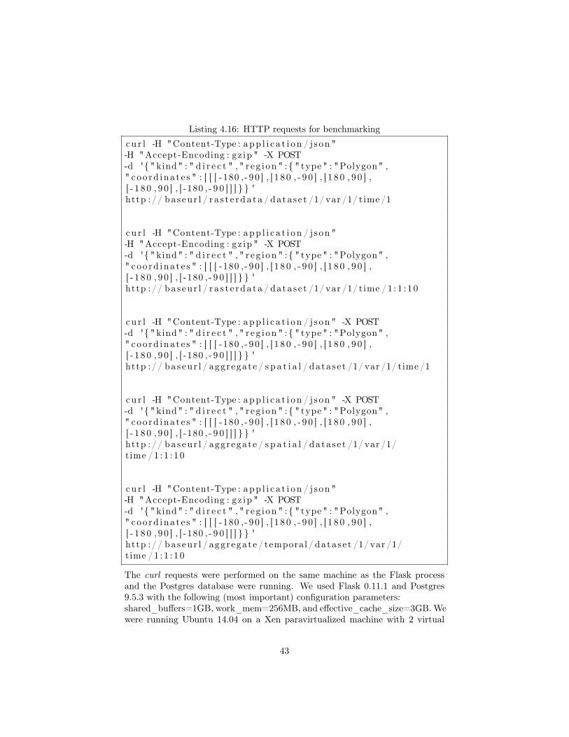
Listing 4.16: HTTP requests for benchmarking

cu r l -H "Content-Type : app l i c a t i o n / j son "-H "Accept-Encoding : gz ip " -X POST-d '{ "kind" : " d i r e c t " , " r eg i on " : { " type" : "Polygon" ," coo rd ina t e s " : [ [ [ -180 ,- 9 0 ] , [ 1 8 0 , - 9 0 ] , [ 1 8 0 , 9 0 ] ,[ - 1 8 0 , 9 0 ] , [ -180 ,- 9 0 ] ] ] } } 'http :// bas eu r l / r a s t e rda ta / datase t /1/ var /1/ time /1

cu r l -H "Content-Type : app l i c a t i o n / j son "-H "Accept-Encoding : gz ip " -X POST-d '{ "kind" : " d i r e c t " , " r eg i on " : { " type" : "Polygon" ," coo rd ina t e s " : [ [ [ -180 ,- 9 0 ] , [ 1 8 0 , - 9 0 ] , [ 1 8 0 , 9 0 ] ,[ - 1 8 0 , 9 0 ] , [ -180 ,- 9 0 ] ] ] } } 'http :// bas eu r l / r a s t e rda ta / datase t /1/ var /1/ time /1 : 1 : 1 0

cu r l -H "Content-Type : app l i c a t i o n / j son " -X POST-d '{ "kind" : " d i r e c t " , " r eg i on " : { " type" : "Polygon" ," coo rd ina t e s " : [ [ [ -180 ,- 9 0 ] , [ 1 8 0 , - 9 0 ] , [ 1 8 0 , 9 0 ] ,[ - 1 8 0 , 9 0 ] , [ -180 ,- 9 0 ] ] ] } } 'http :// bas eu r l / aggregate / s p a t i a l / datase t /1/ var /1/ time /1

cu r l -H "Content-Type : app l i c a t i o n / j son " -X POST-d '{ "kind" : " d i r e c t " , " r eg i on " : { " type" : "Polygon" ," coo rd ina t e s " : [ [ [ -180 ,- 9 0 ] , [ 1 8 0 , - 9 0 ] , [ 1 8 0 , 9 0 ] ,[ - 1 8 0 , 9 0 ] , [ -180 ,- 9 0 ] ] ] } } 'http :// bas eu r l / aggregate / s p a t i a l / datase t /1/ var /1/time /1 : 1 : 1 0

cu r l -H "Content-Type : app l i c a t i o n / j son "-H "Accept-Encoding : gz ip " -X POST-d '{ "kind" : " d i r e c t " , " r eg i on " : { " type" : "Polygon" ," coo rd ina t e s " : [ [ [ -180 ,- 9 0 ] , [ 1 8 0 , - 9 0 ] , [ 1 8 0 , 9 0 ] ,[ - 1 8 0 , 9 0 ] , [ -180 ,- 9 0 ] ] ] } } 'http :// bas eu r l / aggregate / temporal / datase t /1/ var /1/time /1 : 1 : 1 0

The curl requests were performed on the same machine as the Flask processand the Postgres database were running. We used Flask 0.11.1 and Postgres9.5.3 with the following (most important) configuration parameters:shared_buffers=1GB, work_mem=256MB, and effective_cache_size=3GB.Wewere running Ubuntu 14.04 on a Xen paravirtualized machine with 2 virtual

43

CPUs at 2.2GHz and 4GB virtual RAM. Further, the total data ingested atquery time was five PSIMS NetCDF files (belonging to a single PSIMS dataset)and we set indexes on columns (dataset_id, var_id), (geom), and (time_id) forthe raster_data_single table as well as on columns (dataset_id, var_id) and(geom) for the raster_data_series table.

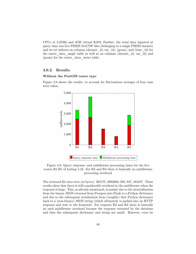
4.6.2 ResultsWithout the PostGIS raster type

Figure 4.8 shows the results, to account for fluctuations averages of four runswere taken.

R1 R2 R3 R4 R50

1,000

2,000

3,000

4,000

5,000

millisecon

ds

Query response time Middleware processing time

Figure 4.8: Query response- and middleware processing times for the fiveroutes R1-R5 of Listing 4.16. For R3 and R4 there is basically no middleware

processing overhead

The returned file sizes were (in bytes): 365175, 2082003, 568, 947, 484107. Theseresults show that there is still considerable overhead in the middleware when theresponse is large. This, as already mentioned, is mainly due to the deserializationfrom the binary JSON returned from Postgres into Flask to a Python dictionaryand due to the subsequent serialization from (roughly) that Python dictionaryback to a (non-binary) JSON string (which ultimately is packed into an HTTPresponse and sent to the frontend). For requests R3 and R4 there is basicallyno such middleware overhead because the response returned by the databaseand thus the subsequent dictionary and string are small. However, even by

44

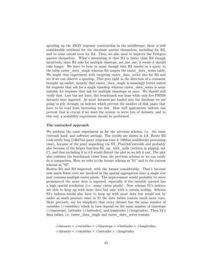
speeding up the JSON response construction in the middleware, there is stillconsiderable overhead for the database queries themselves, including for R3,and to some extent even for R4. Thus, we also need to improve the Postgresqueries themselves. What’s interesting is that R4 is faster than R3 thoughintuitively, since R4 asks for multiple timsteps, not just one, it seems it shouldtake longer. We have to bear in mind though that R3 results in a query tothe table raster_data_single whereas R4 targets the raster_data_series table.We might thus experiment with targeting raster_data_series also for R3 andsee if we can observe a speedup. This goes right in the direction of a commentbrought up earlier, namely, that raster_data_single is seemingly better suitedfor requests that ask for a single timestep whereas raster_data_series is moresuitable for requests that ask for multiple timesteps at once. We should stillverify that. Last but not least, this benchmark was done while only five PSIMSdatasets were ingested. As more datasets are loaded into the database we aregoing to rely strongly on indexes which prevent the number of disk pages thathave to be read from increasing too fast. How well appropriate indexes canprevent that is crucial if we want the system to serve lots of datasets, and tothis end, a scalability experiment should be performed.

The unstacked approach

We perform the same experiment as for the previous schema, i.e. the same(virtual) hard- and software settings. The results are shown in 4.9. Route R2took overly long (14647ms query response time & 1868ms middleware processingtime), because of the pixel unpacking via ST_PixelAsCentroids and probablyalso because of the helper function fill_up_with_nulls (written in plpgsql, notC), and thus including it in 4.9 would distort the plot so we left it out. The plotalso contains the benchmark times from the previous schema so we can easilydo a comparison. Here we refer to the former schema as ”S1” and to the currentschema as ”S2”.Routes R3 and R4 improved, with the former considerably. That’s becausenow much fewer rows are involved in the spatial aggregation since a single rownow contains multiple raster pixels. The improvement would probably be morepronounced the more data is ingested, especially if the variable queried hasa high spatial resolution (i.e. many raster pixels). Now schema S1’s indexesare able to keep up with more data but only with a certain scaling. SchemaS2’s indexes would also have to keep up with more data but would not beunder as much pressure since in S1 the data tables contain much more rows.More precisely, say for simplicity that every dataset has the same number ofvariables (#variables) which in turn depend on the same number of timesteps(#timesteps), latitudes (#latitudes), and longitudes (#longitudes). Then S1’sdata tables, i.e. raster_data_single and raster_data_series contain

#datasets×#variables×#timesteps×#latitudes×#longitudes,#datasets×#variables×#latitudes×#longitudes

45

R1-S1

R1-S2

R3-S1

R3-S2

R4-S1

R4-S2

R5-S1

R5-S2

0

2,000

4,000

6,000

millisecon

ds

Query response time Middleware processing time

Figure 4.9: Query response- and middleware processing times for the routesR1,3,4,5 for schemas S1 and S2

many rows respectively. Contrast this to

#datasets×#variables×#timesteps×#tiles

many rows for S2’s raster_data table, where

#tiles =#latitudestilesizelat

× #longitudestilesizelon

,

where by choosing tilesizelat = O(

1#latitudes

)and tilesizelon = O

(1

#longitudes

)this becomes

O (#datasets×#variables×#timesteps) ,

i.e. independent of #latitudes or #longitudes. Note that while the numberof rows for S1’s raster_data_series table is not independent of #latitudes and#longitudes, it is independent of #timesteps. However, for datasets with a largenumber of timesteps (such as AgMERRA with #timesteps ∼ 10k) where userslikely want to extract only a subset in time, we would be forced to load all thetimesteps for individual pixels because in a database one usually cannot loadrows partially. Also note that we would still have to determine optimal tilesizestilesizelat and tilesizelon. If tilesizelat = 1 = tilesizelon then obviously we fall backto the schema of the S1 raster_data_single table leading to a large number ofrows and thus we would be relying heavily on an index on (latitude,longitude)

46

(or rather PostGIS’ geom) besides indexes on dataset_id, var_id, time_id. Ifhowever we choose tilesizelat, tilesizelon too large, then individual rows will con-tain many raster pixels many of which will not fall into the polygon providedby the user and would have to be filtered out in an extra step, not by an indexitself. To examine this discussion further, the experiment should be repeatedfor varying tilesizes.Next we observe that R5 in 4.9 worsened considerably. This is likely due tothe fact that for pSIMS, the timeseries of values consists entirely of NODATAvalues for most of the pixels and S1’s temporal aggregation query filters outthese pixels very early (through the condition: NOT (values[t1] IS NULL AND· · · AND values[tn] IS NULL)) whereas S2’s temporal aggregation query can-not do such a filtering because the values are packed inside the PostGIS rastertype (we cannot filter out individual pixels if their values are NODATA, wecan only filter out entire raster tiles if all their pixel values are NODATA, i.e.through ST_BandIsNoData). Therefore, a further experiment should be per-formed where the data is dense (e.g. with the AgMERRA dataset), and whereone can probably observe S1’s temporal aggregation query to become slower tothe point where it will be roughly as slow as S2’s.Last but not least, for route R1 the query response times are very similar, yet theoverhead in the middleware is slightly higher for S2. That is probably becauseof a data type conversion. More precisely, for S1 the NetCDF type NC_FLOATis converted to a Python float32 via the netCDF4 library and then inserted intoa Postgres double precision field. Since a Python float32 can only hold up to 9digits the value field in raster_data_single also just has 9 digits at most. ForS2 however, while we still use the Python netCDF4 library for ingestion, thevalues are inserted as a PostGIS raster type with pixeltype 32BF which getsconverted to a Postgres double precision once we call ST_PixelAsCentroids.During that conversion the number of digits expands to 12 for most of the val-ues (for a reason that has to be examined). Thus, in S2 the response returnedby Postgres is actually a little larger than in S1 (368950B VS 365175B) leadingprobably not so much to extra deserialization overhead (when deserializing aPostgres double precision sent over the network inside Flask) but likely to ex-tra serialization and subsequent compression overhead. This however has to beexamined in more depth, in particular we have to track exactly how NetCDFtypes are mapped to Python types and from there to Postgres types. This willbecome necessary anyway once we handle more diverse NetCDF files that donot just have NC_FLOAT variables but also NC_DOUBLE or NC_INT, ornon-numeric types such as NC_CHAR (in which case we should probably de-cide whether to even ingest such a variable in the first place because at least S1only handle NetCDF types that can be exactly represented by a double preci-sion, because the value field in the raster_data_single table is of Postgres typedouble precision (and similarly for the values field in the raster_data_seriestable)).Shortly, if we are to represent a variety of NetCDF data types in a databasethen there are basically two approaches. Either we have a database column ofdifferent type for every new NetCDF data type or we use a general enough type

47

that can represent all the NetCDF data types without loss of accuracy and storethe finer type information additionally, e.g. use a Postgres double precision torepresent NC_INT, NC_FLOAT, NC_DOUBLE, yet store the fact that theywere actually NC_INT, NC_FLOAT, NC_DOUBLE in order to truncate un-necessary digits when returning data to the user. However, if we also have toaccommodate non-numeric NetCDF types such as NC_CHAR in a Postgresdouble precision field then it will be more cumbersome since we would have todo type conversions ourselves using SQL.Although not fully examined yet, the data type conversion issue is probably alsothe reason why the JSON responses (the largest ones being gzipped, see 4.16)for routes R1-R5 are different in size. For S1 the response sizes are (in bytes),as mentioned before: 365175, 2082003, 568, 947, 484107, whereas for S2 theyare: 368950, 2143323, 568, 945, 471914.

4.7 A more general API and Postgres schemaThe HTTP API and the Postgres schemas described so far only support NetCDFvariables that depend on (time, lat, lon) but not on say (lat, lon), (vertical, lat,lon), (time, vertical, lat, lon). While variables depending on (lat, lon) couldsomewhat be accommodated by having the time_id column be NULL this ap-proach is clearly not desirable. Similarly, NetCDF variables that depend on(vertical, lat, lon) could also be accommodated somewhat by using the time_idcolumn also for the vertical axis, and in this respect rename it to say some-thing like ’z_id’ where the ’z’-direction can stand for time or vertical axis. Butcertainly when we consider NetCDF variables that depend on (time, vertical,lat, lon) then the schemas described so far cannot handle them. Thus, we needa more general database schema to handle all these various NetCDF variablesthat depend on various axes. The same goes for the HTTP API where clientsshould be able to slice a variable not just along the time axis but also alongthe vertical axis if the variable does indeed depend on a vertical axis. Thus, tomake the HTTP API more general, i.e. to allow for more general slicing alongmultiple axes, one should put the slicing arguments (i.e. so far time_id_start,time_id_step, time_id_end, time_id) into the POST JSON body as well,and likely one can put other future route arguments into this body as well. Inthis section we thus present a more general HTTP API as well as a more generaldatabase schema as an important step towards supporting much more diverseNetCDF datasets. We note that not only were the schemas presented so far notgeneral enough but neither did they represent the NetCDF data model correctly.In particular, the former schemas attributed to much meaning to NetCDF di-mensions whereas really they are merely indexes consisting of a name and a size,nothing more.

48

4.7.1 A more general Postgres schemaGeneral Remarks

Figure 4.10 shows the new general schema that is able to accommodate manymore NetCDF datasets than the schemas discussed so far. First we note thatthere is a dataset and a variable table similar to the raster_datasets andraster_variables tables from the previous schemas. All other tables store the”actual” data and are very similar to the raster_data_single table from thewithout_raster_type schema. However, these data tables fall into two cate-gories, one to the right of the variable table and one to the left. The data tableson the right have no understanding of time, vertical, latitude, longitude, theyonly consider the NetCDF variables as multi-dimensional arrays with meaning-less indexes index_0, index_1, index_2, index_3, etc. which directly cor-respond to the variable’s dimensions in the NetCDF file. The data tables onthe left however do have an understanding of time, vertical, latitude, longi-tude, as we can already see from the column names time_value, time_stamp,vertical_value, geom. These columns index the actual raster pixel values,which are just the value columns, but via meaningful axes as opposed to themeaningless indexes used in tables on the right.The purpose of the data tables on the right is that they support OpENDAP-likeindex-slicing queries on a NetCDF variable. This functionality is the minimalfunctionality we want our schema to support and is also a fall-back support forNetCDF variables to which we cannot associate semantic axes time, vertical,latitude, longitude either because these variables do indeed not depend on suchaxes or because the NetCDF files they belong to do not follow the CF conven-tions in which case the ingestion code won’t be able to detect time, vertical,latitude, longitude axes properly. These data tables also support selecting/s-licing a NetCDF variable ”by value along its dimensions”, however, only if thecorresponding NetCDF dimension has an associated variable (which by defini-tion is a variable that has the same name as the dimension and only dependson the dimension itself). If not then the corresponding value_0, or value_1,value_2, value_3 will be NULL and the user cannot do a range query on that.The purpose of the data tables on the left is that they further support what wecan call selecting/slicing a NetCDF variable ”by value along its axes” as opposedto just ”by index” or ”by value along its dimensions”. What this really meanswe will show with an example soon.We also note that the schema as it is now supports NetCDF variables that de-pend on 1,2,3, or 4 dimensions and if we express their dependency in terms ofaxes, only depends on either (time), (vertical), (lat, lon), (vertical, lat, lon),(time, lat, lon), (time, vertical, lat, lon). However, as we can easily see, theschema is extendable in the sense that if one faces a NetCDF variable whichdepends on 5 or more dimensions (or 0 dimensions) when just looking at itsdimensions, or when looking at its axes on another combination of axes, e.g.(time, lat), then one can simply create additional tables for that which easilyplug into the existing schema.

49

The fact that we use different tables for different dimensionality not only pre-vents us from using lots of NULLs, i.e. say we store all NetCDF variable datain a single table. Then that table should have columns for time, vertical, lat,lon, because it needs to accommodate all variables and in the worst case thereis a variable that depends on all 4 (or even more in the future, we don’t know).Variables however that only depend on (lat, lon) and are stored in this table,would have the time and vertical columns be NULL throughout, a waste of diskspace, and also counter-intuitive.Using different tables for different dimensionality also helps to some extent withscalability since once we know a variable only depends on 3 dimensions we don’thave to filter through data of variables that depend on n dimensions where nis different from 3, i.e. knowing the dimensionality already cuts down the se-lectivity to a single table which only contains the data for variables with thatsame dimensionality.Further we note that the schema supports non-uniform time, vertical, lat, lonbecause we never compress these to just a starting value, step size, and numberof values, but store every individual value.

The variable table

There are some things that must be mentioned about the variable table. First,if one needs to decide in which table a variable’s data is actually stored, thisis done via the type and axes fields. The type is one of T,Z, Y,X, or D. Tmeans it’s a variable that stores time data, Z vertical data (height/depth), Ylatitude, and X longitude (we use the same notation and order as in the CFconventions). D means it’s a ’data’ variable, i.e. a variable such as pressure,temperature, etc. that depends on T,Z, Y,X variables. If a variable’s type isD then all the following columns won’t be NULL and the axes field will thensignify the axes the variable depends on, i.e. (T ), (Z), (T, Y,X), (Z, Y,X),(T,Z, Y,X). A variable’s type might also be NULL meaning that it is either avariable that does indeed not store coordinate data or couldn’t be detected assuch a variable at ingestion time.So to sum up, if say a variable is of type D with axes (T, Y,X) then its datacan be found in the value_time_lat_lon table. Similarly, if a variable’s type isD with axes (Z) then its data is in the value_vertical table. We note that if avariable is of type D then its data is stored twice, once in a corresponding tableto the right of the variable table and once in a corresponding table to the leftof the variable table. If a variable is not of type D then its data only appearsin a table on the right (with fall-back range query support).It is important to realize that the table to be queried depends on the axescolumn (given type is D) which itself depends on the variable to be queried.Thus, if the user issues an HTTP request to get the data for a certain variable,at that point we don’t know yet the table that holds that variable’s data buthave to first examine the axes field of the variable (which we can query sincethe URL contains the variable’s id). This dynamic dispatching to the correcttable is not only cumbersome but probably also not the way one should use a

50

relational database, whatever that means exactly.

Examples

In this section we will go through example NetCDF variables and show in whichtables of Figure 4.10 the data will end up. Say we take for example the aet_whevariable in 2.1. This variable depends on 3 dimensions so its data is certainlygoing to end up in the table value_3d. Since moreover each of the dimensionsit depends on has a corresponding variable (which has the same name and onlydepends on that dimension, i.e. time(time), lat(lat), lon(lon)) the columnsvalue_0, value_1, value_2 will have the corresponding values of these vari-ables, i.e. the table value_3d will hold

• index_0 = index of time dimension = 1, . . . , 34 =: i

• value_0 = time(i)

• index_1 = index of lat dimension = 1, . . . , 360 =: j

• value_1 = lat(j)

• index_2 = index of lon dimension = 1, . . . , 720 =: k

• value_2 = lon(k)

• value = aet_whe(i, j, k)

Since the time, lat, lon variables have the semantics of actual time, latitude,longitude, the aet_whe variable will also be stored in value_time_lat_lonwith

• time_value = time(i)

• time_stamp = absolute timestamp of time(i)

• geom = geom(lat(j), lon(k))

• value = aet_whe(i, j, k)

Now at this point the reader might think what really the difference is betweenthe value_3d and value_time_lat_lon tables and this brings us to the followingsecond example 4.17.

51

Listing 4.17: Output of ncdump -c on an RTOFS NetCDF file

ne tcd f rtofs_glo_2ds_f002_1hrly_diag {dimensions :MT = UNLIMITED ; // (1 cu r r en t l y )Y = 3298 ;X = 4500 ;v a r i a b l e s :double MT(MT) ;MT: long_name = "time" ;MT: un i t s = "days s i n c e 1 9 0 0 1 2 3 1 00 : 00 : 00 " ;MT: ca l endar = " standard " ;MT: ax i s = "T" ;double Date (MT) ;Date : long_name = "date " ;Date : un i t s = "day as %Y%m%d.% f " ;Date : C_format = "%13.4 f " ;Date :FORTRAN_format = " ( f13 . 4 ) " ;

i n t Y(Y) ;Y: point_spacing = "even" ;Y: ax i s = "Y" ;i n t X(X) ;X: point_spacing = "even" ;X: ax i s = "X" ;f l o a t Lat i tude (Y, X) ;Lat i tude : standard_name = " l a t i t u d e " ;Lat i tude : un i t s = "degrees_north " ;

f l o a t Longitude (Y, X) ;Longitude : standard_name = " long i tude " ;Longitude : un i t s = " degrees_east " ;Longitude : modulo = "360 degree s " ;

f l o a t ice_coverage (MT, Y, X) ;ice_coverage : c oo rd ina t e s = "Longitude Lat i tude Date" ;i ce_coverage : standard_name = " sea_ice_area_fract ion " ;ice_coverage : un i t s = "" ;ice_coverage : _Fi l lValue = 1.267651 e+30 f ;i ce_coverage : val id_range = 0 . f , 1 . f ;i ce_coverage : long_name = " i c e coverage [ 9 0 . 9H] " ;

. . .}

If we focus on the variable ice_coverage, then its data will end up in thevalue_3d table with

• index_0 = index of MT dimension = 1, . . . , 1 =: i

• value_0 = MT(i)

52

• index_1 = index of Y dimension = 1, . . . , 3298 =: j

• value_1 = Y(j)

• index_2 = index of X dimension = 1, . . . , 4500 =: k

• value_2 = X(k)

• value = ice_coverage(i, j, k)

However, it will also be stored in the value_time_lat_lon table with

• time_value = MT(i)

• time_stamp = absolute timestamp of MT(i)

• geom = geom(Latitude(j, k), Longitude(j, k))

• value = aet_whe(i, j, k)

That’s because the ice_coverage variable uses auxiliary coordinate variablesLongitude, Latitude, Date (specified through the CF-compliant special-purposecoordinates attribute), so really X,Y aren’t the real longitude, latitude vari-ables, but Longitude, Latitude are (detected as such because of their unitsattribute, not because of their names, which is unreliable, see CF conventions).As a detail note that the variable detected as a proper time variable is MT (notDate) because it is the one that has a valid time units attribute (as specifiedin the CF conventions).Now at this point the reader might still not be convinced about why the dis-tinction into tables on the right and tables on the left of the variable table isuseful. To this end, let us consider a final example, Example H.1 in the CFconventions CF-1.6. For such a NetCDF file the variable humidity would endup in the value_1d table because strictly counting the number of dimensionsthis variable depends on we get 1. Thus, value_1d would contain

• index_0 = index of obs dimension = 1, . . . , 1234 =: i

• value_0 = NULL (because the obs dimension does not have a correspond-ing variable)

• value = obs(i)

However, since the humidity variable has the variables time, alt, lat, lon associ-ated (through the CF-compliant special-purpose attribute coordinates, see CFconventions), semantically, it is a variable which depends on T,Z, Y,X, and thusits data will also be stored in the value_time_vertical_lat_lon table with

• time_value = time(i)

• time_stamp = absolute timestamp of time(i)

53

• vertical_value = alt(i)

• geom = geom(lat(i), lon(i))

• value = humidity(i)

Thus, with this example it should finally be clear why we need both the tableson the right, which don’t have an understanding of T,Z, Y,X but merely con-sider NetCDF variables strictly as multi-dimensional arrays without associatingto them variables with special meaning, whereas the tables on the left do exactlythat. If a NetCDF file is CF-compliant its variables will end up in both kinds oftables allowing for richer query capability. If a NetCDF file is not CF-compliantor it just has variables to which we cannot associate T,Z, Y,X variables, thenits data will only be in a table on the right allowing for less query capability butstill supporting fall-back range queries on dimension indices (the kinds OpEN-DAP supports) and also on values of corresponding variables if there are suchvariables.

4.7.2 A more general HTTP APIAlong with a more general database schema we of course also need a moregeneral HTTP API implemented in the EDE Flask code component of Figure3.1. This API is specified in ede_rest_api this time not yet as API Blueprintfiles but just as JSON files, specifying request and response formats. We herebriefly discuss the main points of these formats.

Get a dataset’s metadata

Response format: response_dataset.jsonGET /rastermeta/datasets/dataset_id

Return the metadata of a specific dataset. If no dataset is specified, the meta-data of all datasets currently present in the backend is returned. The returnedmetadata of a dataset contains its uid, global attributes, dimensions, and vari-ables. The variables are distinguished into ”axis variables” and ”data variables”.The former are variables that are T,Z, Y , or X, the latter are variables that de-pend on the former. For all variables we return its minimum and maxium valuesand for a data variable we additionally return the axis variables it depends onas well as its bounding box (which is the coverage of non-NODATA respectivelynon-NULL values) in case Y,X is among the axis variables it depends on.

The response format in particular contains all variables in the dataset with theiruid’s. These in turn a client can use to issue subsequent requests for the routesbelow.

54

Get a variable’s metadata

Response format: response_variable.jsonGET /rastermeta/variables/variable_id

Return the metadata of a specific variable. If no variable is specified, the meta-data of all variables currently present in the backend is returned. The returnedmetadata of a variable in particular contains its uid, the dataset it belongs to,its type, and if it’s a data variable the axis variables it depends on. Also, as forthe previous route we also return the variable’s bounding box (in case Y,X isamong the axis variables it depends on).

The response format in particular contains the uid of the dataset the variablebelongs to so that a user can easily navigate back to the dataset with a subse-quent request.

Select a variable’s data

Request format: request_select.jsonResponse format: response_select.jsonPOST /rasterdata/vars/variable_id

In the request JSON a user can specify filters on axis variables a data variabledepends on, i.e. if a data variable say depends on T,Z, Y,X then the user canspecify a filter on T , one on Z, and one on Y,X combined. We decided tohave the filter on Y,X be combined because a polygonal restriction on Y,X ismore general than the cross-product of a range restriction on Y with a rangerestriction on X. More precisely, a filter is an axis variable together with arestriction on that axis variable. A restriction in turn consist of a form andparameters. In case the axis variable is T or Z the form is either single (incase the user wants to pinpoint to a single value) or a range (in case the userwants to specify a range of values). In case the axis variable is Y,X the form iseither direct (in case the user wants to specify a polygonal restriction directly)or indirect (in case the user wants to specify a polygonal restriction indirectly,i.e. by specifying a uid which points to a polygon stored in the backend itself).We also note that for a T axis the parameters field also has a type which iseither relative or absolute. In case it’s relative the times are specified as thenumeric values which appear in the NetCDF file, e.g. 14 days since 1970-01-01,the 14 would be the value. In case it’s absolute the times are specified as abso-lute timestrings, i.e. 1970-01-15. This allows for more user-friendly querying.

In the response JSON we return the filters the user specified in the requestitself, and then of course metadata about the variable. More importantly wereturn the actual raster pixel values as an array of points where each point hasan array associated to it (in case the variable depends on T, Y,X or Z, Y,X)or a matrix (in case the variable’s axes are T,Z, Y,X), or just a single value

55

(in case the variable just depends on Y,X). This main information is stored inthe data field of the response JSON. However, the user needs to know what theactual values for T and/or Z are which is why we return that information inthe values attribute of the corresponding axis variable, i.e. if e.g. the variabledepends on T, Y,X and a point in the data field has the array of values

[227.949996948, 230.050003052, 224.850006104, 232.25, 234.350006104],

then we need to know which times correspond to these values. These timescan be found in the valuesRelative (specified as relative times) respectivelyvaluesAbsolute (specified as absolute times) field of the variable’s T axis, i.e.we then know that the corresponding times for these values are

[46720.0416667, 46721.0416667, 46722.0416667, 46723.0416667, 46724.0416667]

signifying ”days since 1860-01-01 00:00:00”, respectively the more human-friendlyabsolute timestrings

["1987-12-01 01:00:00-06", "1987-12-02 01:00:00-06", "1987-12-03 01:00:00-06","1987-12-04 01:00:00-06", "1987-12-05 01:00:00-06"].

Lastly, the field min is a variable’s minimum value yet only within the selectionspecified whereas globalMin is a variable’s global minimum value, i.e. over thevariable’s entire range without any selection restriction, similarly for max andglobalMax, and for a T axis we further distinguish between the usual relativeand absolute, i.e. there is minRelative, globalMinRelative, minAbsolute,globalMinAbsolute, and accordingly for max.

Aggregate a variable’s data

Request format: request_aggregate.jsonResponse format: response_aggregate.jsonPOST /aggregate/vars/variable_id

The request and response JSONs for this route are very similar to the requestand response JSONs for the selection route, the main difference being that forthis aggregation route one also specifies the axis over which to aggregate andthe kind of aggregation operation to perform.

56

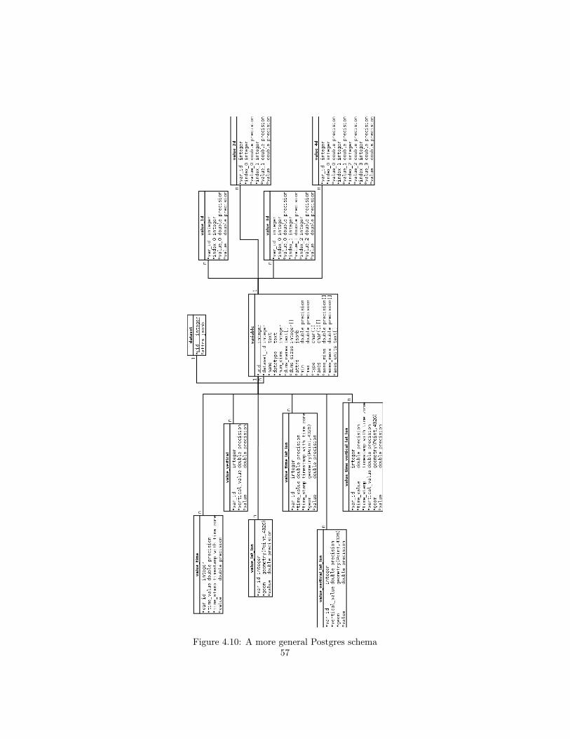
Figure 4.10: A more general Postgres schema57