Storage opportunity loss with a Pearson demand distribution

ELSEVIER

international journal of

production economics

Int. J. Production Economics 35 (1994) 351-357

Storage opportunity loss with a Pearson demand distribution

H. Pastijn”, M. Schaffers

Royal Military Academ!,, Renaissance A~wm~ 30. B-1040 Brussrls, Brlgium

Abstract

In the past, we investigated the influence of some demand distribution functions on the minimum expected storage opportunity loss. This investigation was restricted in two ways. First, it concerned the expected opportunity loss function with linear components due to under- or over-dimensioning of the storage level. Secondly, it concerned only symmetric Pearson demand distribution functions. This paper generalizes the previous results for a very wide range of Pearson distributions.

1. Introduction

A lot of engineering and management problems are concerned with the dimensioning of one decision variable in a context of uncertainty. Examples are currently found in civil engineering, budgetting, warehousing and storage management.

Generally, we observe three different types of approaches, often according to the technological tradition in the field of the applications.

Type I. The best guess of the variable is cal- culated, based upon standard computational rules. Afterwards, a certain amount is added to make it extremely unlikely to underestimate the required value. This heuristical method implies no explicit risk evaluation, but merely the introduction of the so-called safety coefficient. It is often used in civil engineering.

Type II. The value of the variable is determined in order to limit the risk of over- or under-estima-

* Corresponding author

tion. This method requires the knowledge of a distribution function. In storage management, this approach is leading to the concept of a safety stock. This method requires no cost knowledge.

Type 111. The value of the decision variable is obtained by optimizing an opportunity loss function. This method requires the knowledge of eco- nomic aspects of over- and under-estimation as well as a distribution function.

The applicability of these different types depends only on the amount of knowledge we have about the phenomenon we are dealing with.

If one has knowledge about the probalistic demand distribution, as well as about the cost of over- or under-estimation of the demand, then both types II and III approaches are encountered in storage management. In this sense the dimensioning of the required stock level of an item, in order to meet the (probabilistic) demand is generally treated in practice as a mono-criterium problem, either of type II or of type III. If it is of type III, then it is considered traditionally in the literature as the newspaper-boy problem: determine the amount of

0925-5273/94/$07.00 (0 1994 Elsevier Science B.V. All rights reserved

SSDI 0925-5273(93)00140-Q

352 H. Pmtijn, M. Sch&r.s/Int. J. Production Economics 35 (1994) 351-357

newspapers to take in stock in order to minimize the expected loss due to under- or over-estimation of the probahstic demand. This problem has been solved computationally for some symmetric demand distributions (for the normal distribution and for the uniform distribution) and for a few discrete ones. We already discussed the sensitivity of the optimization results for a wide range of symmetric Pearson distributions (see [ 11).

This sensitivity analysis has two main motiva- tions. First, the knowledge of the demand distributions is not always very accurate in reality. So it is interesting to know the effect of the departure from “normally” on the optimization results. Second, in practice one is often looking at the problem as it were of type II. So it is interesting to have an idea of the influence of the departure from type III optimality according to the different demand distributions.

These arguments motivated us to generalize the discussion of the sensitivity of the optimization problem of type III for a very wide range of Pear- son distributions, by dropping the symmetry char- acteristic of the demand distribution.

In this paper, we will constrain the discussion to a linear cost structure of the opportunity loss, as it is in the traditional newspaper-boy problem.

2. The opportunity cost

A management problem is defined by, on one side, a model of the demand, and, on the other side, a model of the cost of under- or of over-estimation of the demand.

The demand is a random variable, whose distribution is specified by a probability density function (pdf). By convention, this function is assumed to be zero outside the possible range of the random variable. In this paper, this pdf, denoted by .f; will always be a Pearson distribution, which is entirely specified by the values of the parameters ,u, g, /?i, and ,!?? (respectively the mean, standard deviation, symmetric and kurtosis coefficients). See for instance [2] for an introduction to those distributions.

The cost will be the function c, linear in the under- or over-estimation of the demand. So the

function c is governed by the two positive parameters k, and k,, in the following way:

c(x) = i

- k,x (x < 0),

k,x (x 3 0),

if x is the excess of the estimation (the stock) over the actual demand.

We will denote the quantity in stock by L, and the demand by 8.

The value of the expected cost @ of the storage management problem, for a distribution f and a cost function c, with a fixed stock L is given by the formula

+ x,

Q(L) = f(U)c(L - H)dH.

-x

This function is always continuous, and decreasing in a first part and increasing in the other part of the real axis - its derivative is monotonously increasing ~ if the cost function c has this property.

Clearly, this property is conserved if we take a positive linear combination of such functions. Indeed, the derivative of the combination is the positive linear combination of the derivative, and is therefore monotonously increasing if the original functions are. So for any sampling

of the real axis, the function

C.ftdiJctL - Oi)tHi - di- 1)

is first decreasing, then increasing, since the function c has this property, and since the coefficients in the expression are positive.

But the function Qi is the limit of such an expression, and therefore has also this property.

We conclude that the function @ has at most a closed interval of minima, which are always global, and which will be reduced in our case to one point. So the minimization problem is well stated. We will denote this unique global minimum by L*,

and its corresponding value by

@* = @(L*).

H. Pastijn, M. Schaff‘rrsjlnt. J. Production Economics 35 (1994J 351-357 353

In our case, the expression of the expected (opportunity loss) cost is

L + n

Q(L) =

s f(O)k,(L - 8)d0 +

s f(@k,(0 - L)d0

-r L

+a,

= k, i,,u,,L - O)dO + k, jf(B)(H - L)dG.

-z L

This minimum satisfies the necessary condition

&Q(L) = 0,

which in our case becomes

+S

k, jf(“)do + k, jf(O)dQ = 0.

-n; L

If the cumulative probability distribution function (cpdf) is

-x

then the necessary condition can be rewritten as

k,F(L*) - k,(l - F(L*)) = 0,

or

F&C*) = &. 0 ”

If we define K to be

K + 0

then we have

F(L*) = &.

Usually in the literature it is assumed that the demand is normally distributed.

The purpose of this paper is to examine to what extent the departure from this normality hypothesis

is influencing the optimization results. Therefore, the sensitivity investigation is carried out in a very wide range of Pearson demand pdfs.

So we will study how the optimal expected cost Cp depends, on one hand, on the parameters p, CS, pi, and pZ, and, on the other hand, on the parameters k, and k,.

Not all these parameters are relevant to our study.

Let

be the optimal value

@* = @(L*)

where the demand pdf is a Pearson function with parameters fii, fi2, p, 0 and where the cost function c is specified by the coefficients k, and k,.

It is well-known that iff(Q) is a Pearson pdf with parameters p, CT, /I1 and b2 and if

0 ’

then

is also a Pearson distribution with parameters ~1 = 0, CJ = 1, pi and fi2. In this context i should be called the reduced demand variable.

As a consequence, if the cost function c(x) is positively homogeneous, in the sense that for any positive scalar Z, we have

c(crx) = K(X),

then we have

Since in our case c(x) is positively homogeneous, the parameters p and 0 are not relevant for our study. In the next sections, the discussion is limited to ~1 = 0 and CJ = 1, and consequently the notation

@*(Bi,D2,p,g.,k,,k,)

will be replaced by

@*(B,>B,>k,,k,).

3. The symmetric case

The symmetric distributions are characterized by a parameter /I1 = 0.

Those distributions were also studied in [l] and what follows can be seen as a continuation of this previous study.

Obviously,

@*(Br,lj2,ko,ku)= k,@*(B,,LLt,K),

with

What we are interested in is what will be the distance between the value @* for any distribution and the corresponding one for a normal distribution, which is characterized by the parameters

p, =o

and

[j2 = 3.

So we want to study the function

Y(K) = @*(Bl?L 1, K)

@*(o, 3,1, K)

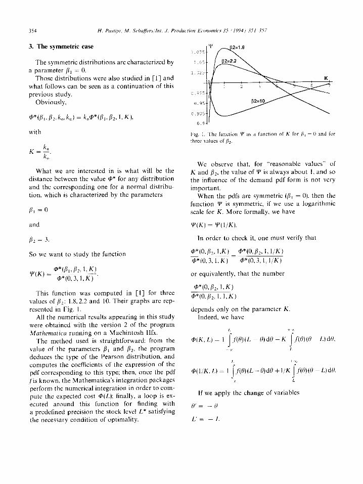
This function was computed in [l] for three values of fiZ: l&2.2 and 10. Their graphs are represented in Fig. 1.

All the numerical results appearing in this study were obtained with the version 2 of the program Muthematica running on a Machintosh Ilfx.

The method used is straightforward: from the value of the parameters PI and bZ, the program deduces the type of the Pearson distribution, and computes the coefficients of the expression of the pdf corresponding to this type; then, once the pdf

,J’is known, the Mathematics’s integration packages perform the numerical integration in order to com- pute the expected cost Q(L); finally, a loop is ex- ecuted around this function for finding with a predefined precision the stock level L* satisfying the necessary condition of optimality.

Fig. I. The function y/ as a function of K for p, = 0 and for

three values of PI.

We observe that, for “reasonable values” of K and jIZ, the value of Y is always about 1, and so the influence of the demand pdf form is not very important.

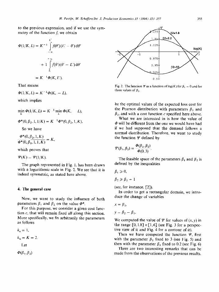
When the pdfs are symmetric (fir = 0), then the function Y is symmetric, if we use a logarithmic scale for K. More formally, we have

Y(K) = ‘Y(l/K).

In order to check it, one must verify that

@*(o,B2,l.K) @*(0,/L f,l/‘K)

@*(0,3,l,K) = @*(0,3,1,1/K)

or equivalently, that the number

@*(0,/L 1,K)

@*(O,Bz,l, 1,K)

depends only on the parameter K. Indeed. we have

I. + )rl

@(K,L) = 1 I

j’(H)(L - B)d0 + K i

f(O)(I) -L)dU,

-1 I.

I. + 9,

@(l/K,L) = 1 j’(o)@-0)dH +1/K .f‘(U)(O -L)dlI. i s

_X L

If we apply the change of variables

c)‘= -0

L’= -,I_

H. Pasrijn, hf. Sehaffersllnt. J. Production Economies 35 (1994) 351-357 355

to the previous expression, and if we use the symmetry of the functionf, we obtain

L’

@(l/E&L) = K-’ s

f(e’)(L’ - 8’)d@

+ 1 c f(&)(@ - L’) de’

= K-‘@(K,L’).

That means

@(l/K,L) = K- ‘@(K, - L),

which implies

mjn @(l/K, L) = Km ’ m,‘n @(K, - L),

@*(O,P,, 1,1/K) = Km’@*(0,fi2, 1,K).

So we have

@*(O, fiz, 1, K)

@*(O,p,, 1, 1, K) = K’

which proves that

Y(K) = Y(l/K).

The graph represented in Fig. 1, has been drawn with a logarithmic scale in Fig. 2. We see that it is indeed symmetric, as stated here above.

4. The general case

Now, we want to study the influence of both parameters pi and fi2 on the value @J*.

For this purpose, we consider a given cost function c, that will remain fixed all along this section. More specifically, we fix arbitrarily the parameters as follows

k,= 1,

k, = K = 2.

Let

Fig. 2. The function Y as a function of log(K) for fi, = 0 and for

three values of bz.

be the optimal values of the expected loss cost for the Pearson distribution with parameters pi and /12, and with a cost function c specified here above.

What we are interested in is how the value of @ will be different from the one we would have had if we had supposed that the demand follows a normal distribution. Therefore, we want to study the function Y defined by

The feasible space of the parameters pi and f12 is defined by the inequalities

P* 30,

(see, for instance, [2]). In order to get a rectangular domain, we intro-

duce the change of variables

x = Bl,

Y = B2 - Pl.

We computed the value of !Y for values of (x, y) in the range [0,1.8] x [ 1,6] (see Fig. 3 for a perspective view of it and Fig. 4 for a contour of it).

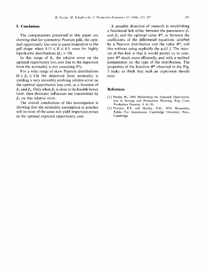
Then we have computed the function Y, first with the parameter pz fixed to 3 (see Fig. 5) and then with the parameter /?i fixed to 0.2 (see Fig. 6)

There are two interesting remarks that can be made from the observations of the previous results.

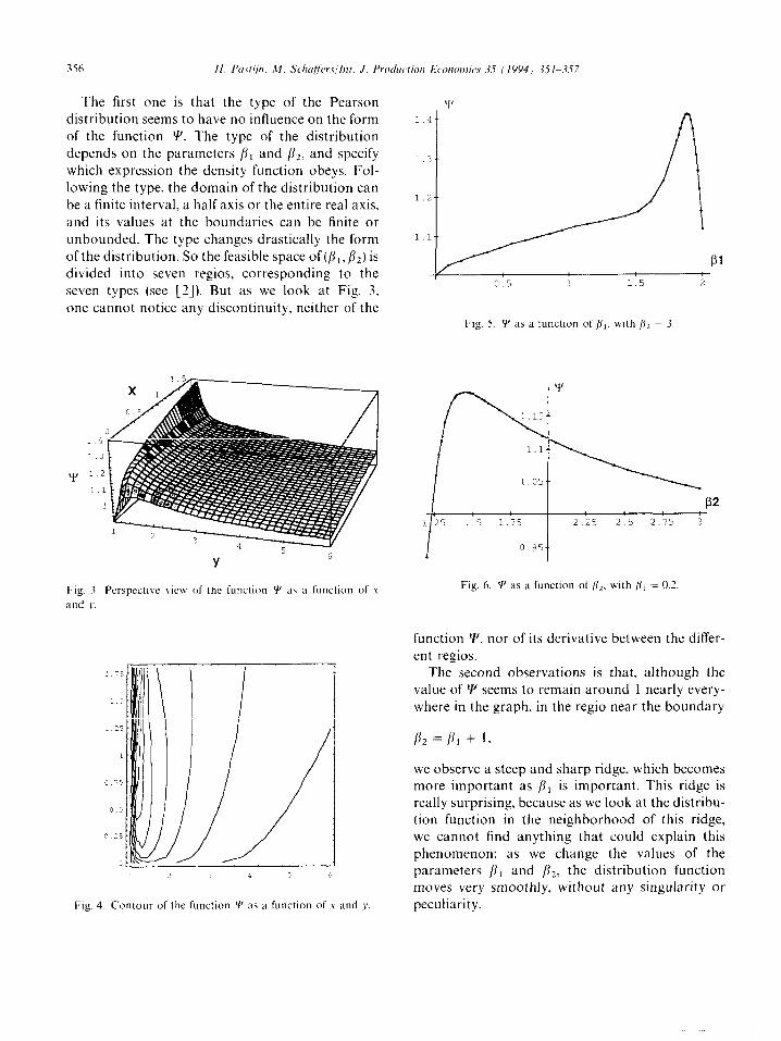
The first one is that the type of the Pearson distribution seems to have no influence on the form of the function Y. The type of the distribution depends on the parameters /I1 and fi2, and specify which expression the density function obeys. Fol- lowing the type, the domain of the distribution can be a finite interval, a half axis or the entire real axis, and its values at the boundaries can be finite or unbounded. The type changes drastically the form of the distribution. So the feasible space of (p,, fiz) is divided into seven regios, corresponding to the seven types (see 121). But as we look at Fig. 3, one cannot notice any discontinuity, neither of the

1 ‘1

I.’

1.2

1.1

i.4

1.3

Y 1.2

1.1

Y

Fig. 3. Perspective view of the function Y’ a~ a function of .x

;tnd .I’

Fig. 4. Contour of the function Y as a function of Y and y.

‘I’

/A Pl

0.5 1 1.5 2

Fig. 5. Y as a function of /Il. with /fL = 3

P2 1 25 1.5 1.75 2.25 2.5 2.75 3

I 0.95 t Fig. 6. ‘f’ as a function of [j2. with /iI = 0.2.

function Y, nor of its derivative between the different regios.

The second observations is that, although the value of Y seems to remain around 1 nearly every- where in the graph, in the regio near the boundary

we observe a steep and sharp ridge, which becomes more important as /I, is important. This ridge is really surprising, because as we look at the distribution function in the neighborhood of this ridge, we cannot find anything that could explain this phenomenon: as we change the values of the parameters p, and p2. the distribution function moves very smoothly, without any singularity or peculiarity.

H. Pastijn. M. Schu/j%vs~It~t. J. Produuc~tion Economics 35 (1994) 351-357 357

5. Conclusions

The computations presented in this paper are showing that for symmetric Pearson pdfs, the optimal opportunity loss cost is quasi insensitive to the pdf shape when 0.15 < K 6 6.5, even for highly leptokurtic distributions (p2 = 10).

In this range of K, the relative error on the optimal opportunity loss cost due to the departure from the normality is not exceeding 8%.

For a wide range of skew Pearson distributions (0 -$ /3i < 1.8) the departure from normality is yielding a very smoothly evolving relative error on the optimal opportunity loss cost, as a function of pi and p2. Only when f12 is close to its feasible lower limit, then dramatic influences are transmitted by pi on this relative error.

The overall conclusions of this investigation is showing that the normality assumption in practice will in most of the cases not yield important errors in the optimal expected opportunity cost.

A possible direction of research is establishing a functional link either between the parameters /jl and pz and the optimal value @*, or between the coefficients of the differential equations satisfied by a Pearson distribution and the value @*, and this without using explicitly the p.d.f. ,1: The inter- est of this link is that it would permit us to com- pute @* much more efficiently, and with a method independent on the type of the distribution. The properties of the function @* observed in the Fig. 3 make us think that such an expression should exist.

References

fll

VI

Pastijn, H., 1985. Minimizing the Expected Opportunity

loss in Storage and Production Planning. Eng. Costs

Production Econom., 9: 41-50.

Pearson, ES. and Hartley, H.O., 1954. Biometrika

Tables For Statisticians. Cambridge University Press, Cambridge.

Documents

Storage opportunity loss with a Pearson demand distribution