STOPPING SIGHT DISTANCE AND HORIZONTAL …docs.trb.org/prp/14-1723.pdf · Wood, J.S. & Donnell, E.T. 1 TRB 2014 Annual Meeting 1 INTRODUCTION 2 Stopping sight distance and horizontal

TRB 2014 Annual Meeting

STOPPING SIGHT DISTANCE AND HORIZONTAL SIGHTLINE

OFFSETS AT HORIZONTAL CURVES

Jonathan S. Wood (Corresponding Author)

Graduate Research Assistant

Department of Civil and Environmental Engineering

The Pennsylvania State University

839 Ashworth Lane

Boalsburg, PA 16827

Phone: (435) 760-2781

Fax: (814) 863-7304

Email: [email protected]

Eric T. Donnell

Associate Professor

Department of Civil and Environmental Engineering

The Pennsylvania State University

231 Sackett Building

University Park, PA 16802

Phone: (814) 863-7053

Fax: (814) 863-7304

Email: [email protected]

Submitted for presentation and publication consideration to 2014 TRB Annual Meeting

5,732 words + (250*4 Figures) + (250*3 Tables) = 7,482 words

Submission date: November 15, 2013

TRB 2014 Annual Meeting Paper revised from original submittal.


ABSTRACT 1 Horizontal curve design criteria implicitly rely on the design speed to produce safe and efficient 2

designs. This is particularly true for horizontal sightline offsets and stopping sight distance 3

criteria. Current design guidance provides a method for calculating minimum horizontal 4

sightline offsets, but is only accurate and valid when both the driver and object are within the 5

limits of the curve. Other methods are available to estimate minimum horizontal sightline offsets 6

when the driver and/or object are not within the curve limits. However, design guidance 7

recommends using the calculated value for offsets as a conservative estimate near the ends of 8

curves. 9

Speed prediction models and reliability theory were used to estimate the probability that 10

drivers would not have enough sight distance to see, react to, and stop before reaching an object 11

in the roadway if applying horizontal sightline offset criteria when the driver or object are 12

outside the limits of a horizontal curve. Six different scenarios at the approach to a curve and 13

inside the curve were analyzed. Reliability estimates based on minimum horizontal sightline 14

offsets (using current minimum design criteria) and stopping sight distance distributions based 15

on individual driver characteristics show that the probability of drivers not having enough 16

stopping sight distance is much greater at the approach than inside horizontal curves. To 17

improve the consistency of designs, it is suggested that the calculated horizontal sightline offsets 18

be used beyond the limits of the curve (approach and departure tangents) to provide extra sight 19

distance for drivers near the curve. 20


Wood, J.S. & Donnell, E.T. 1


INTRODUCTION 1 Stopping sight distance and horizontal sightline offset are considered important design criteria 2

for safe roadway designs and are included in the Federal Highway Administration’s (FHWA) 3

thirteen controlling criteria (1). Horizontal sightline offsets at sharp horizontal curves are often 4

controlled by the minimum stopping sight distance for a given design speed. Current design 5

guidance for minimum stopping sight distance is a function of the design speed, driver 6

perception-reaction times, and driver deceleration rates (2, 3). While the assumed reaction times 7

and deceleration rates are conservative estimates, the design speed is often lower than the actual 8

operating speed of a given road segment (4). For a minimum stopping sight distance, at any 9

point along a curve, there is a minimum horizontal sightline offset. Current design methods for 10

calculating minimum horizontal sightline offsets along horizontal curves are valid only when 11

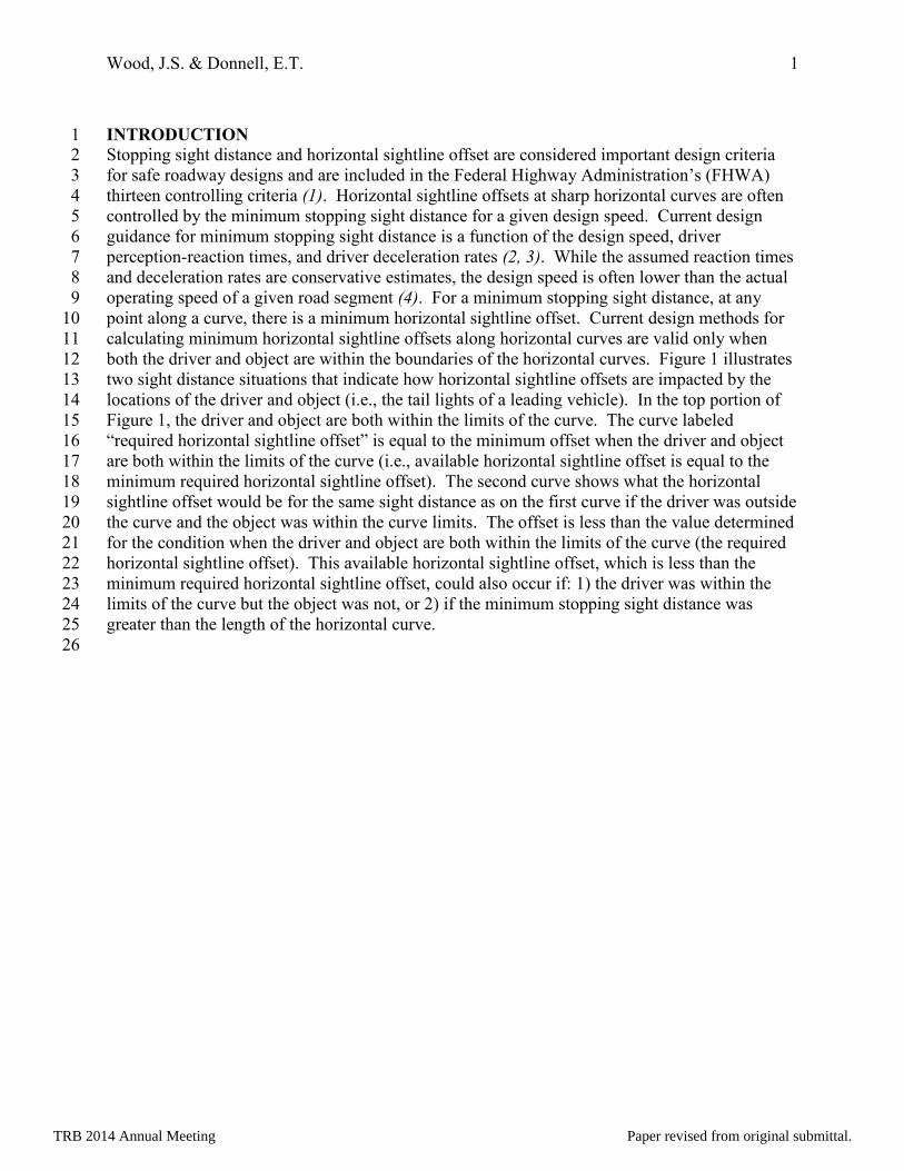
both the driver and object are within the boundaries of the horizontal curves. Figure 1 illustrates 12

two sight distance situations that indicate how horizontal sightline offsets are impacted by the 13

locations of the driver and object (i.e., the tail lights of a leading vehicle). In the top portion of 14

Figure 1, the driver and object are both within the limits of the curve. The curve labeled 15

“required horizontal sightline offset” is equal to the minimum offset when the driver and object 16

are both within the limits of the curve (i.e., available horizontal sightline offset is equal to the 17

minimum required horizontal sightline offset). The second curve shows what the horizontal 18

sightline offset would be for the same sight distance as on the first curve if the driver was outside 19

the curve and the object was within the curve limits. The offset is less than the value determined 20

for the condition when the driver and object are both within the limits of the curve (the required 21

horizontal sightline offset). This available horizontal sightline offset, which is less than the 22

minimum required horizontal sightline offset, could also occur if: 1) the driver was within the 23

limits of the curve but the object was not, or 2) if the minimum stopping sight distance was 24

greater than the length of the horizontal curve. 25

26




FIGURE 1 Horizontal Sightline Offsets and Sight Distance 1 2

Current design methods for estimating minimum horizontal sightline offsets when the 3

driver, the object, or both are outside the limits of the curve include a manually intensive 4

graphical technique (straight-line method) and a computational method that was developed in 5

1972. Little is known in regards to how the aforementioned computational method from 1972 6

was developed or how accurate it is (5). The American Association of State Highway and 7

Transportation Officials’ (AASHTO) A Policy on Geometric Design of Highways and Streets 8

(herein referred to as the Green Book) recommends using the calculated offsets as conservative 9




estimates for locations near the ends of horizontal curves (3). It has been pointed out that using 1

these conservative estimates could lead to higher project costs than necessary due to the need to 2

remove existing buildings, trees and vegetation, or side-slope cut areas (5). The safety impacts 3

of providing less than minimum stopping sight distance has been explored (2, 6, 7, 8, 9, 10); 4

however, all of these studies were limited to the effects of stopping sight distance on vertical 5

curves. The safety impacts of providing the minimum stopping sight distance based on 6

published research are conflicting, indicating that there are no safety impacts associated with 7

providing more sight distance (2, 6), that safety performance worsens as sight distance increases 8

(7), or that safety improves as sight distance increases (8, 9, 10). No studies investigating the 9

safety effects of providing less than the minimum stopping sight distances contained in the Green 10

Book for horizontal curves were found. Also, the safety impacts associated with providing 11

stopping sight distances that exceed the minimum values contained in the Green Book have not 12

been compared to the safety performance of roadways with precisely the minimum stopping 13

sight distance at horizontal curves. 14

This paper describes and discusses some of the issues relating to how using the 15

conservative estimate for providing the minimum stopping sight distance near the ends of curves 16

impacts horizontal curve design. 17

DESIGN METHODS 18

Design Speed and Design Consistency 19 Green Book design methods rely on the concept of selecting a design speed, and then using this 20

selected speed to determine minimum or limiting values for various roadway features. Design 21

speeds are supposed to be logical, anticipate the operating speed, and be as high as practical in 22

order to attain safety, mobility, and efficiency within project constraints (3). Selected design 23

speeds should fit the travel desires and behavior of nearly all drivers and should be a high-24

percentile value in the free-flow speed distribution (3). Design speed is particularly important 25

for the design of horizontal curves as it is used explicitly to determine the minimum radius of 26

curve, superelevation, and minimum stopping sight distance. The Green Book notes that there 27

should not be restrictions placed on sight distances or the use of flatter curves where they can be 28

provided as part of an economical design (3). 29

Once the design speed for a road is determined, designers are encouraged to use the 30

highest practical values possible for design criteria (e.g. the largest radius for a horizontal curve) 31

on high-speed facilities (3). The Green Book cautions that use of above minimum design criteria 32

on road segments with lower design speeds may encourage drivers to travel at speeds higher than 33

the design speed (3). This is consistent with research findings that observed 85th

percentile 34

speeds tend to be higher than the design speed for rural two-lane highways with design speeds 35

that are below 55 mph (11). Design assessment tools have been developed that attempt to reduce 36

the variability in operating speeds that result from the design process. These methods rely on 37

alignment indices, speed distribution parameters (mean operating speed, 85th

percentile operating 38

speed, and speed variance), and driver workload estimates (12, 13, 14). These methods predict 39

speeds for successive design features along a given road segment in order to produce road 40

segments with homogenous driver operating speeds and performance. 41

42




(1)

Horizontal Sight Offsets and Stopping Sight Distance 1 The Green Book provides an objective method to calculate the minimum horizontal sightline 2

offset, as shown in Equation 1 below (3). The horizontal sightline offset is the distance between 3

the center of the innermost lane on the road and a sight obstruction. This distance must be clear 4

in order to provide a specified stopping sight distance for a given curve radius. Equation 1 was 5

developed based on the geometry of a simple circular curve and, as previously mentioned, is 6

only accurate when both the driver and object on the roadway are within the limits of the curve 7

(i.e., between the point of curvature and point of tangency) as shown in Figure 1. 8

[

] 9

Where 10

HSO = the minimum horizontal sight offset from the center of the innermost lane in ft; 11

R = the radius of the center of the innermost lane in ft; and 12

S = the minimum stopping sight distance in ft. 13

14

The straight-line method suggested in the Green Book can estimate the available sight 15

distance (the distance available that drivers can see an object on the roadway) for situations 16

where either the driver or the object is outside the curve and the other is within the curve, but this 17

method is error prone and tedious (5). For existing single roadside objects near the ends of 18

curves, this is often the best option if the offset to the object is not as large as the offset 19

calculated using Equation 1. 20

The computational method suggested by the Green Book can also deal with the same 21

issues as the straight-line method but is not readily available to most designers, was mainly 22

developed for spiral curves, and it is not understood how accurate the method is (5). This is 23

likely the best method for checking available sight distance, when available to the designer, if the 24

horizontal curve involves a spiral curve and the offset desired is less than the conservative value 25


For continuous roadside objects near the ends of curves, a designer must determine 27

whether to provide the minimum stopping sight distance all the way around the curve or whether 28

to provide extra sight distance at the ends of the curve. Extra stopping sight distance can be 29

provided near the ends of curves by using the value calculated from Equation 1. This is 30

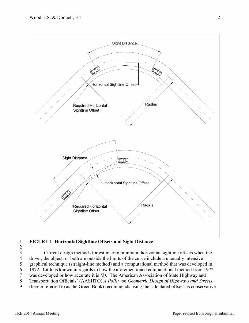
particularly true for curves on roads with lower design speeds. Using Equation 1, Figure 2 31

shows how the minimum horizontal sightline offset varies depending on the radius of curve and 32

design speed. As shown in Figure 2, the minimum offset increases significantly as the radius 33

decreases at lower design speeds; whereas, for higher design speeds, the horizontal sightline 34

offset increases at a much slower rate as the radius decreases. Thus, the potential budget savings 35

(in percent of total project cost) is likely to be highest for projects involving low design speed 36

road segments. The overall cost savings is likely to be highest on projects with high design 37

speeds if the conservative values are not used towards the ends of the curves and other methods 38

are used to reduce the minimum horizontal sightline offsets. However, the difference between 39

the offsets found using Equation 1 and the other two methods are often not significant (3). 40

41




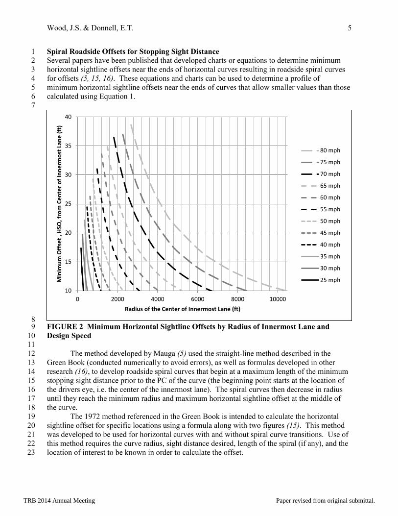
Spiral Roadside Offsets for Stopping Sight Distance 1 Several papers have been published that developed charts or equations to determine minimum 2

horizontal sightline offsets near the ends of horizontal curves resulting in roadside spiral curves 3

for offsets (5, 15, 16). These equations and charts can be used to determine a profile of 4

minimum horizontal sightline offsets near the ends of curves that allow smaller values than those 5


7

8 FIGURE 2 Minimum Horizontal Sightline Offsets by Radius of Innermost Lane and 9

Design Speed 10 11

The method developed by Mauga (5) used the straight-line method described in the 12

Green Book (conducted numerically to avoid errors), as well as formulas developed in other 13

research (16), to develop roadside spiral curves that begin at a maximum length of the minimum 14

stopping sight distance prior to the PC of the curve (the beginning point starts at the location of 15

the drivers eye, i.e. the center of the innermost lane). The spiral curves then decrease in radius 16

until they reach the minimum radius and maximum horizontal sightline offset at the middle of 17

the curve. 18

The 1972 method referenced in the Green Book is intended to calculate the horizontal 19

sightline offset for specific locations using a formula along with two figures (15). This method 20

was developed to be used for horizontal curves with and without spiral curve transitions. Use of 21

this method requires the curve radius, sight distance desired, length of the spiral (if any), and the 22

location of interest to be known in order to calculate the offset. 23

10

15

20

25

30

35

40

0 2000 4000 6000 8000 10000

Min

imu

m O

ffse

t , H

SO,

fro

m C

en

ter

of

Inn

erm

ost

Lan

e (

ft)

Radius of the Center of Innermost Lane (ft)

80 mph

75 mph

70 mph

65 mph

60 mph

55 mph

50 mph

45 mph

40 mph

35 mph

30 mph

25 mph




A method to calculate stopping sight distance for any point along an approach tangent, 1

departure tangent, or within a curve given an object with a specific horizontal sight offset at a 2

particular location was developed in 1987 (16). The relationships for this method used the curve 3

radius, horizontal sightline offsets, and lengths related to the driver location, object location, and 4

curve to derive formulas that can be used to calculate the available sight distance for any point of 5

interest near or within a curve. 6

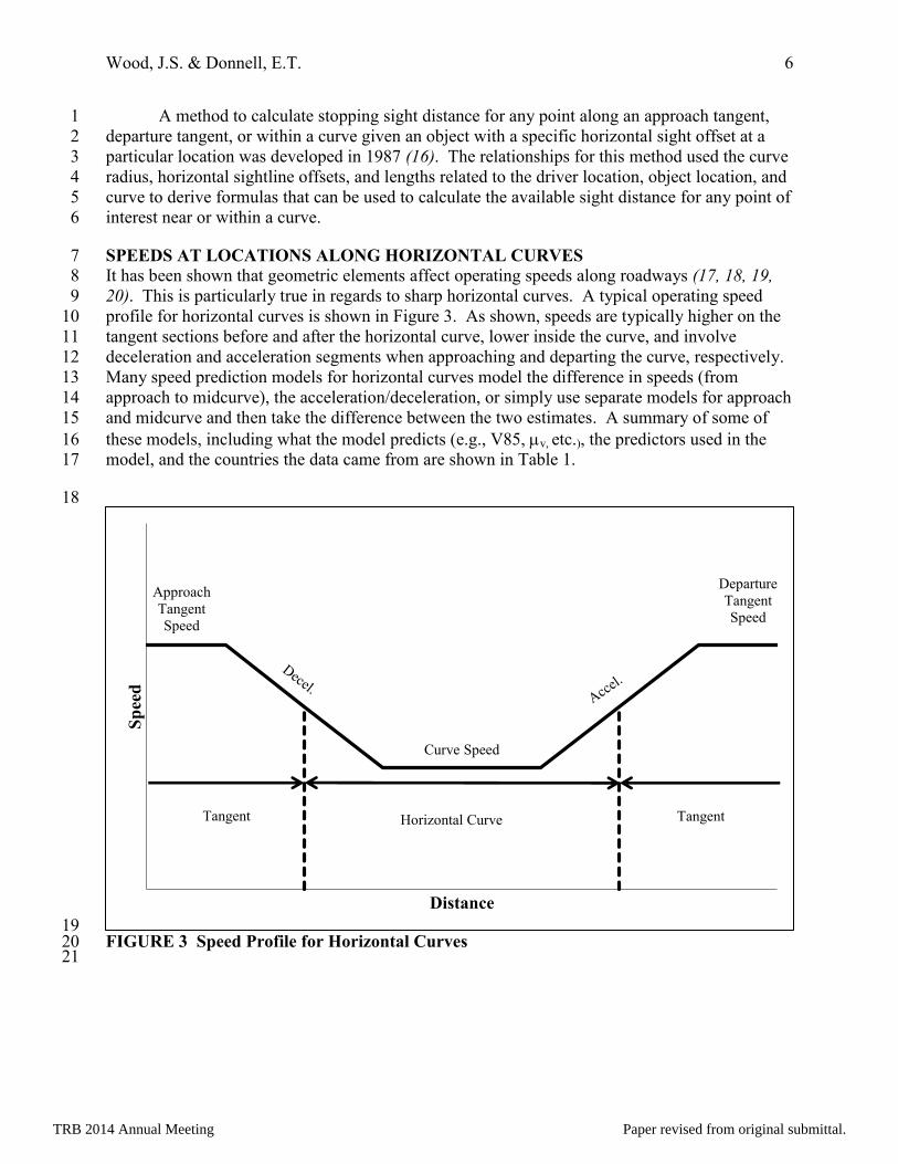
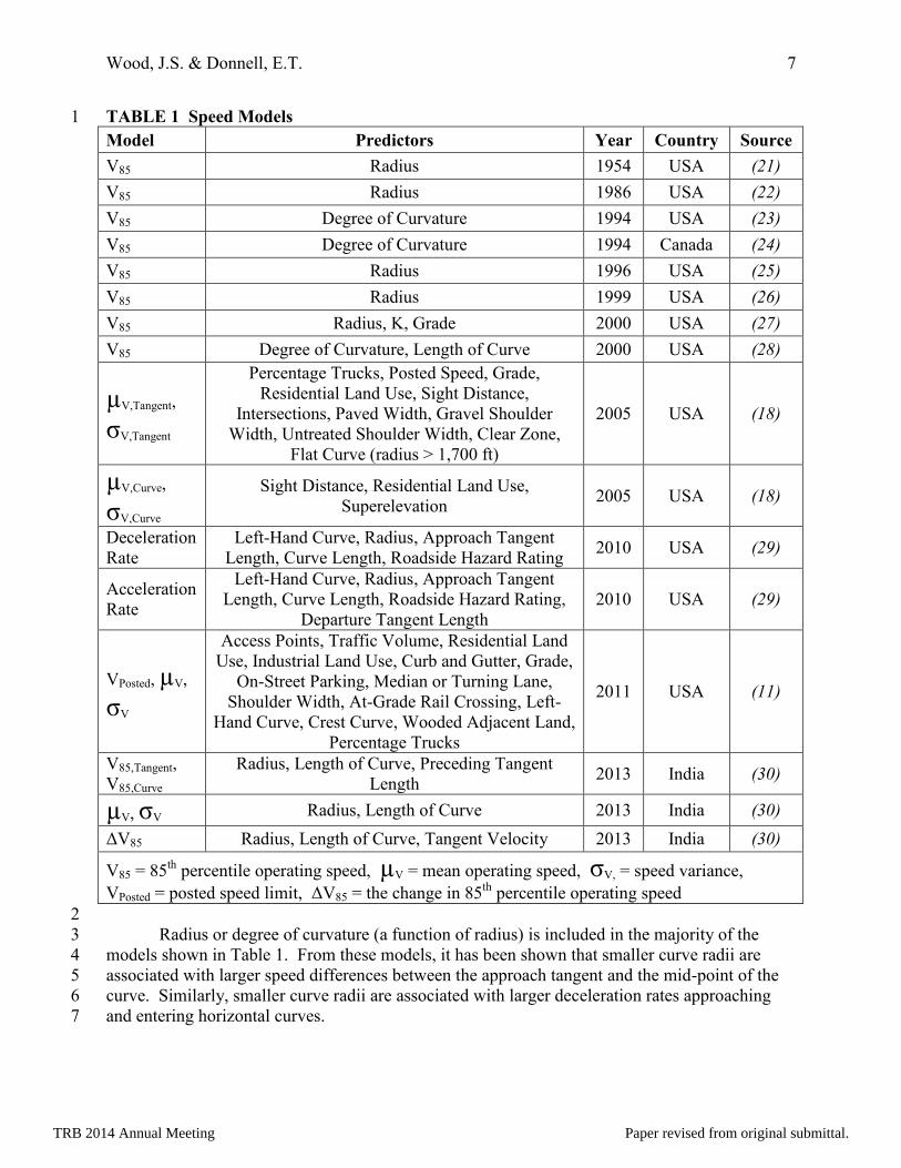
SPEEDS AT LOCATIONS ALONG HORIZONTAL CURVES 7 It has been shown that geometric elements affect operating speeds along roadways (17, 18, 19, 8

20). This is particularly true in regards to sharp horizontal curves. A typical operating speed 9

profile for horizontal curves is shown in Figure 3. As shown, speeds are typically higher on the 10

tangent sections before and after the horizontal curve, lower inside the curve, and involve 11

deceleration and acceleration segments when approaching and departing the curve, respectively. 12

Many speed prediction models for horizontal curves model the difference in speeds (from 13

approach to midcurve), the acceleration/deceleration, or simply use separate models for approach 14

and midcurve and then take the difference between the two estimates. A summary of some of 15

these models, including what the model predicts (e.g., V85, v, etc.), the predictors used in the 16

model, and the countries the data came from are shown in Table 1. 17

18

19 FIGURE 3 Speed Profile for Horizontal Curves 20 21

Approach

Tangent

Speed

Curve Speed

Departure

Tangent

Speed

Sp

eed

Distance

Tangent Tangent Horizontal Curve




TABLE 1 Speed Models 1

Model Predictors Year Country Source

V85 Radius 1954 USA (21)


V85 Degree of Curvature 1994 USA (23)

V85 Degree of Curvature 1994 Canada (24)



V85 Radius, K, Grade 2000 USA (27)

V85 Degree of Curvature, Length of Curve 2000 USA (28)

µV,Tangent,

σV,Tangent

Percentage Trucks, Posted Speed, Grade,

Residential Land Use, Sight Distance,

Intersections, Paved Width, Gravel Shoulder

Width, Untreated Shoulder Width, Clear Zone,

Flat Curve (radius > 1,700 ft)

2005 USA (18)

µV,Curve,

σV,Curve

Sight Distance, Residential Land Use,

Superelevation 2005 USA (18)

Deceleration

Rate

Left-Hand Curve, Radius, Approach Tangent

Length, Curve Length, Roadside Hazard Rating 2010 USA (29)

Acceleration

Rate

Left-Hand Curve, Radius, Approach Tangent

Length, Curve Length, Roadside Hazard Rating,

Departure Tangent Length

2010 USA (29)

VPosted, µV,

σV

Access Points, Traffic Volume, Residential Land

Use, Industrial Land Use, Curb and Gutter, Grade,

On-Street Parking, Median or Turning Lane,

Shoulder Width, At-Grade Rail Crossing, Left-

Hand Curve, Crest Curve, Wooded Adjacent Land,

Percentage Trucks

2011 USA (11)

V85,Tangent,

V85,Curve

Radius, Length of Curve, Preceding Tangent

Length 2013 India (30)

µV, σV Radius, Length of Curve 2013 India (30)

ΔV85 Radius, Length of Curve, Tangent Velocity 2013 India (30)

V85 = 85th

percentile operating speed, µV = mean operating speed, σV, = speed variance,

VPosted = posted speed limit, ΔV85 = the change in 85th

percentile operating speed

2

Radius or degree of curvature (a function of radius) is included in the majority of the 3

models shown in Table 1. From these models, it has been shown that smaller curve radii are 4

associated with larger speed differences between the approach tangent and the mid-point of the 5

curve. Similarly, smaller curve radii are associated with larger deceleration rates approaching 6

and entering horizontal curves. 7




Stopping sight distance has been shown to have a statistically significant association 1

with vehicle speeds (18). The findings indicate that as available sight distance increases, the 2

average speeds within a curve increase. The findings also indicate that speeds along tangent 3

sections preceding curves had a quadratic relationship with speed, including an overall increase 4

in average speeds as available sight distance increased. No statistically significant relationship 5

between available sight distance and speed variance was found for either location. It was found 6

that locations with a wider roadside clear zone had lower speed variance along the approach 7

tangent. 8

PROBABILITY OF NON-COMPLIANCE 9

Methods 10 Reliability theory has been used extensively in civil engineering applications to analyze and 11

create load and resistance factor design criteria (31), analyze and make reliability based decisions 12

on aging bridges (32), asses and estimate safety factors for existing structures (33, 34), analyze 13

water distribution networks (35, 36), and to analyze water resource allocation problems (37). It 14

has been used on a smaller scale in transportation engineering applications, but has been 15

suggested for use in transportation safety applications when crash modification factors are not 16

available for a design element or treatment (38). For this paper, reliability theory was used to 17

calculate the probability that a driver would not have enough sight distance to react and stop 18

given an object on the road for the two situations shown in Figure 1. These situations include, 19

for each case, when 1) the driver is approaching a curve and the object is within the limits of a 20

curve and, 2) the driver and object are both within the limits of the curve. The driver and object 21

are both in the innermost lane for all cases analyzed. The reliability was computed using the 22

equation for stopping sight distance and the distribution parameters (mean and standard 23

deviation, where applicable) for the variables in the equation. The equation for stopping sight 24

distance is given by the Green Book as shown in Equation 2 (3). 25

26

27

Where 28

SSD = stopping sight distance in ft; 29

V = the velocity of a vehicle in ft/s; 30

a = deceleration rate in ft/s2; 31

g = 32.2 ft/s2;

32

G = the average grade (decimal); and 33

tr = reaction time in seconds. 34

35

Minimum stopping sight distance is the distance required for a driver to perceive and react to an 36

object, and then stop. This distance varies from driver to driver depending on the operating 37

speed, perception-reaction time, deceleration rate, and the average grade. Reliability theory 38

specifies that the performance function (in this case, Equation 2 for stopping sight distance) be 39

used and that the mean value and standard deviation for the performance function be calculated. 40

The mean value for the performance function was calculated by using the mean values for V, a, 41

and tr along with the values for G (a constant that was specific to the case being analyzed) and g 42

(( ) )

(2)




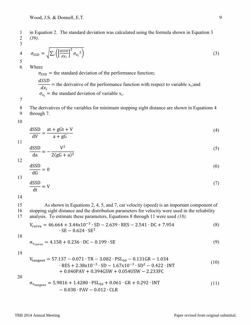
in Equation 2. The standard deviation was calculated using the formula shown in Equation 3 1

(39). 2

3

√∑ ([

]

) (3) 4

5

Where 6

the standard de iation of the performance f nction

the deri ati e of the performance f nction with respect to aria le i and

the standard de iation of aria le i

7

The derivatives of the variables for minimum stopping sight distance are shown in Equations 4 8

through 7. 9

10

(4)

11

( )

(5)

12

(6)

13

(7)

14

As shown in Equations 2, 4, 5, and 7, car velocity (speed) is an important component of 15

stopping sight distance and the distribution parameters for velocity were used in the reliability 16

analysis. To estimate these parameters, Equations 8 through 11 were used (18). 17

(8)

18

(9)

19

(10)

20

(11)




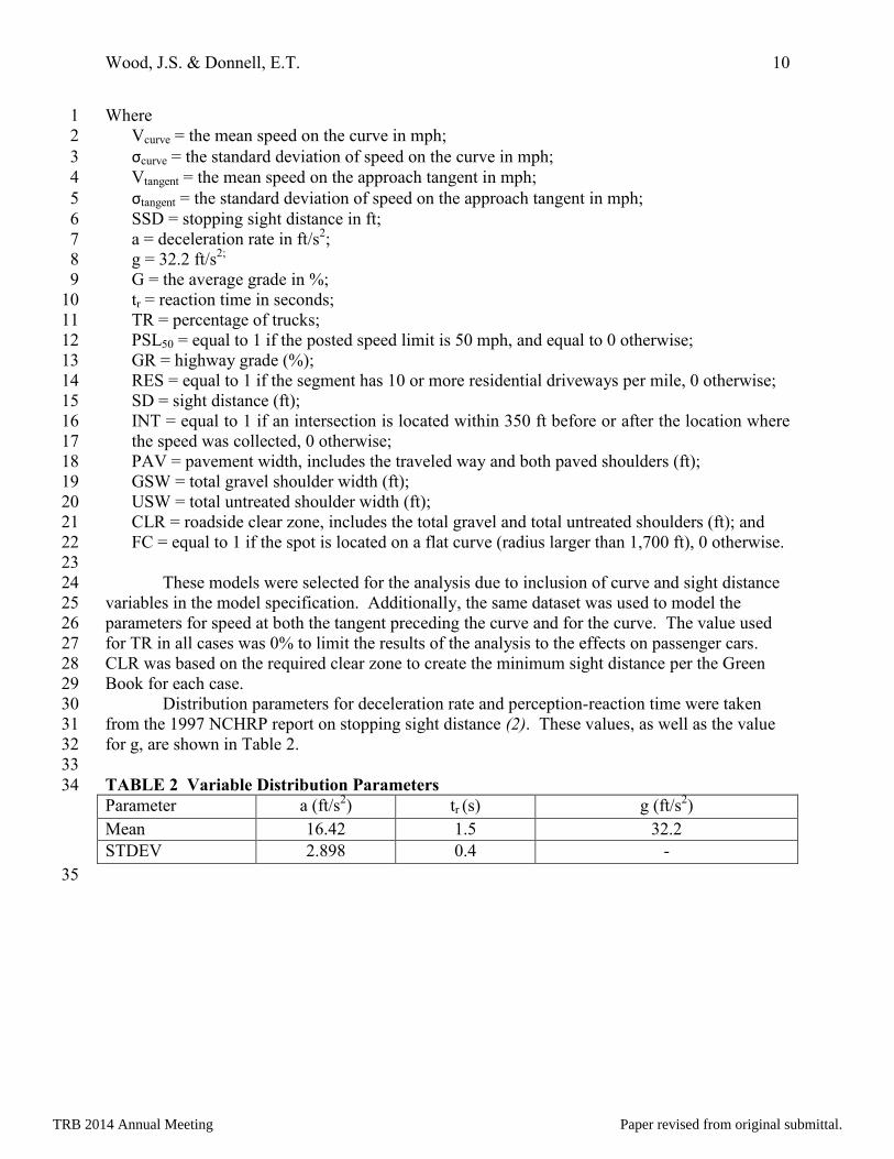
Where 1

Vcurve = the mean speed on the curve in mph; 2

σcurve = the standard deviation of speed on the curve in mph; 3

Vtangent = the mean speed on the approach tangent in mph; 4

σtangent = the standard deviation of speed on the approach tangent in mph; 5

SSD = stopping sight distance in ft; 6

a = deceleration rate in ft/s2; 7

g = 32.2 ft/s2;

8

G = the average grade in %; 9

tr = reaction time in seconds; 10

TR = percentage of trucks; 11

PSL50 = equal to 1 if the posted speed limit is 50 mph, and equal to 0 otherwise; 12

GR = highway grade (%); 13

RES = equal to 1 if the segment has 10 or more residential driveways per mile, 0 otherwise; 14

SD = sight distance (ft); 15

INT = equal to 1 if an intersection is located within 350 ft before or after the location where 16

the speed was collected, 0 otherwise; 17

PAV = pavement width, includes the traveled way and both paved shoulders (ft); 18

GSW = total gravel shoulder width (ft); 19

USW = total untreated shoulder width (ft); 20

CLR = roadside clear zone, includes the total gravel and total untreated shoulders (ft); and 21

FC = equal to 1 if the spot is located on a flat curve (radius larger than 1,700 ft), 0 otherwise. 22

23

These models were selected for the analysis due to inclusion of curve and sight distance 24

variables in the model specification. Additionally, the same dataset was used to model the 25

parameters for speed at both the tangent preceding the curve and for the curve. The value used 26

for TR in all cases was 0% to limit the results of the analysis to the effects on passenger cars. 27

CLR was based on the required clear zone to create the minimum sight distance per the Green 28

Book for each case. 29

Distribution parameters for deceleration rate and perception-reaction time were taken 30

from the 1997 NCHRP report on stopping sight distance (2). These values, as well as the value 31

for g, are shown in Table 2. 32

33

TABLE 2 Variable Distribution Parameters 34

Parameter a (ft/s2) tr (s) g (ft/s

2)

Mean 16.42 1.5 32.2

STDEV 2.898 0.4 -

35




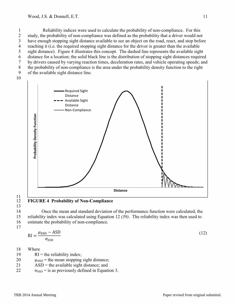
Reliability indices were used to calculate the probability of non-compliance. For this 1

study, the probability of non-compliance was defined as the probability that a driver would not 2

have enough stopping sight distance available to see an object on the road, react, and stop before 3

reaching it (i.e. the required stopping sight distance for the driver is greater than the available 4

sight distance). Figure 4 illustrates this concept. The dashed line represents the available sight 5

distance for a location; the solid black line is the distribution of stopping sight distances required 6

by drivers caused by varying reaction times, deceleration rates, and vehicle operating speeds; and 7

the probability of non-compliance is the area under the probability density function to the right 8

of the available sight distance line. 9

10

11 FIGURE 4 Probability of Non-Compliance 12 13

Once the mean and standard deviation of the performance function were calculated, the 14

reliability index was calculated using Equation 12 (39). The reliability index was then used to 15

estimate the probability of non-compliance. 16

17

(12)

Where 18

RI = the reliability index; 19

µSSD = the mean stopping sight distance; 20

ASD = the available sight distance; and 21

σSSD = is as previously defined in Equation 3. 22

Pro

bab

ility

De

nsi

ty F

un

ctio

n

Distance

Required SightDistance

Available SightDistance

Non-Compliance




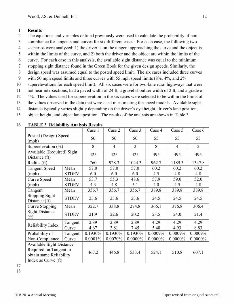
Results 1

The equations and variables defined previously were used to calculate the probability of non-2

compliance for tangents and curves for six different cases. For each case, the following two 3

scenarios were analyzed: 1) the driver is on the tangent approaching the curve and the object is 4

within the limits of the curve, and 2) both the driver and the object are within the limits of the 5

curve. For each case in this analysis, the available sight distance was equal to the minimum 6

stopping sight distance found in the Green Book for the given design speeds. Similarly, the 7

design speed was assumed equal to the posted speed limit. The six cases included three curves 8

with 50 mph speed limits and three curves with 55 mph speed limits (8%, 4%, and 2% 9

superelevations for each speed limit). All six cases were for two-lane rural highways that were 10

not near intersections, had a paved width of 24 ft, a gravel shoulder width of 2 ft, and a grade of -11

4%. The values used for superelevation in the six cases were selected to be within the limits of 12

the values observed in the data that were used in estimating the speed models. Available sight 13

distance typically varies slightly depending on the dri er’s eye height, dri er’s lane position, 14

object height, and object lane position. The results of the analysis are shown in Table 3. 15

TABLE 3 Reliability Analysis Results 16

Case 1 Case 2 Case 3 Case 4 Case 5 Case 6

Posted (Design) Speed

(mph) 50 50 50 55 55 55

Superelevation (%) 8 4 2 8 4 2

Available (Required) Sight

Distance (ft) 425 425 425 495 495 495

Radius (ft) 760 928.3 1044.3 962.7 1189.3 1347.8

Tangent Speed

(mph)

Mean 57.0 57.0 57.0 60.2 60.2 60.2

STDEV 6.0 6.0 6.0 4.5 4.8 4.8

Curve Speed

(mph)

Mean 53.7 55.3 48.6 57.9 59.0 52.0

STDEV 4.3 4.8 5.1 4.0 4.5 4.8

Tangent

Stopping Sight

Distance (ft)

Mean 356.7 356.7 356.7 389.8 389.8 389.8

STDEV 23.6 23.6 23.6 24.5 24.5 24.5

Curve Stopping

Sight Distance

(ft)

Mean 322.7 338.8 274.8 366.1 376.8 306.4

STDEV 21.9 22.6 20.2 23.5 24.0 21.4

Reliability Index Tangent 2.89 2.89 2.89 4.29 4.29 4.29

Curve 4.67 3.81 7.45 5.48 4.93 8.83

Probability of

Non-Compliance

Tangent 0.1930% 0.1930% 0.1930% 0.0009% 0.0009% 0.0009%

Curve 0.0001% 0.0070% 0.0000% 0.0000% 0.0000% 0.0000%

Available Sight Distance

Required on Tangent to

obtain same Reliability

Index as Curve (ft)

467.2 446.8 533.4 524.1 510.8 607.1

17

18




The tangent speed and curve speed parameters shown in Table 3 are the estimated values 1

that were used to calculate the stopping sight distance mean and standard deviation at both the 2

tangent and curve. These values, along with the available sight distance, were then used to 3

calculate the reliability indices. The reliability indices were then converted into the probability 4

of non-compliance. Finally, the amount of sight distance required along the tangent nearing the 5

curve that was needed to produce a reliability index that was the same as that computed for 6

vehicles and objects within the limits of the curve was calculated for each case. 7

As shown in the results, the probability of non-compliance is much greater for the 8

tangents than the curves when the minimum stopping sight distance is provided on the tangent 9

approaching the horizontal curve (e.g. 0.1930 percent vs. 0.0001 percent). The last row in Table 10

3 shows the amount of stopping sight distance that would be required at the approach of the 11

curve in order to have the same low probability of non-compliance as inside the curve. This 12

additional sight distance could be attained by using the offset estimate found using Equation 1 13

near the ends of the curve rather than using roadside spiral offsets. 14

The probability of non-compliance for all cases presented in this section is low (less than 15

0.2% for the tangents and less than or equal to 0.007% for the curves). In practical terms this 16

means that, given that there is an object on the roadway, 1 in 518 drivers on the approach tangent 17

for the first three cases would not have enough sight distance available to see the object, react to 18

it, and come to a stop before reaching it. For drivers on the approach tangent in the last three 19

cases, 1 in 111,000 drivers would not have enough sight distance. For drivers in the curves, 1 in 20

1,000,000 drivers for the first case, 1 in 14,285 drivers in the second case, and essentially 0 21

drivers in cases 3 through 6, would not have enough stopping sight distance available. 22

CONCLUSIONS 23 The operating speed profile is an important concept in geometric design. Current design policy 24

does not explicitly consider this concept and relies on the assumption that establishing a design 25

speed will accommodate operating speed variability. The concept of design consistency has 26

been proposed and provides designers with a tool that incorporates a speed profile into the 27

analysis, but this tool is not required for design and is not used extensively. 28

Horizontal curve design criteria rely on the design speed to result in safe and efficient 29

designs, as currently established. Speed prediction models and reliability theory were used to 30

estimate the probability that drivers would not have enough sight distance to see, react to, and 31

stop before reaching an object in the roadway for six different scenarios at both the approach to a 32

curve and inside the curve if only the minimum stopping sight distance was provided at each 33

location (i.e. if spiral curve offsets were used to make the available sight distance equal to the 34

minimum stopping sight distance). The available sight distance near and along horizontal curves 35

is the distance that is available to drivers with specific eye heights and object heights, and with 36

specific driver and object locations within the lane. For the analysis in this paper, the effects of 37

the variations in these parameters were assumed to be negligible. 38

Results from the reliability analysis indicate that the probability of non-compliance is 39

much greater at the approach to curves than inside horizontal curves. In order to improve the 40

consistency of reliability, it is suggested that the offsets used inside the curve for meeting 41

stopping sight distance requirements be used near the ends of the curve to provide extra sight 42

distance for drivers approaching or departing the curve. 43

One of the potential benefits to estimating the reliability index for stopping sight distance 44

is that it could potentially be used as a design consistency measure. This would require that 45

speed models be used along with geometric data to calculate the reliability indices for the 46




approaches and inside the curves for consecutive curves along a roadway segment. Such models 1

could be included in design consistency software such as the Interactive Highway Safety Design 2

Model (IHSDM). However, before this is done, research establishing whether there is a link 3

between stopping sight distance reliability and safety performance should be conducted. 4

REFERENCES 5

1. FHWA. Federal Aid Policy Guide, Subchapter G - Engineering and Traffic Operatiosn, Part

625 - Design Standards for Highways. FHWA, U.S. Department of Transportation, 1997.

2. D. Fambro, K. Fitzpatrick and R. Koppa. Determination of Stopping Sight Distances,

NCHRP Report 400. Transportation Research Board, Washington DC, 1997.

3. AASHTO. A Policy on Geometric Design of Highways and Streets. American Association

of State Highway and Transportation Officials, 2011.

4. R. Porter, E. Donnell and J. Mason. Geometric Design, Speed, and Safety. In

Transportation Research Record: Journal of the Transportation Research Board, No 2309,

Transportation research Board of the National Acadamies, Washington, D.C., 2012, pp. 39-

47.

5. T. Mauga. Extension of the AASHTO Model for Horizontal Sightline Offset to Apply to

Beginnings and Ends of Simple Horizontal Curves. Presented at 92nd

Annual Meeting of the

Transportation Research Board, Washington, D.C., 2013.

6. P. Olsen, D. Cleveland, P. Fancher, L. Kostyniuk and L. Schneider. NCHRP Report 270:

Parameters Affecting Stopping Sight Distance. Transportation Research Board, Washington,

D.C., 1984.

7. R. Elvik, A. Hoye, T. Vaa and M. Sorensen. The Handbook fo Road Safety Measures, 2nd

edition. Emerald Group Publishing Limited, Bingley, UK, 2009.

8. A. Montella. Safety Evaluation of Curve Delineation Improvements. In Transportation

Research Record: Journal of the Transportation Research Board, No. 2103, Transportation

research Board of the National Acadamies, Washington, D.C., 2009, pp. 69-79.

9. K. Agent, N. Stamatiadis and S. Jones. Development of Accident Reduction Factors.

Kentucky Transportation Center, Lexington, KY, 1996.

10. K. Agent, L. O'Connell, E. Green, J. Pigman, N. Tollner and E. Thompson. Development of

Methodologies for Identifying Hihg-Crash Locations and Prioritizing Safety Improvements.

Kentucky Transportation Center, Lexington, KY, 2003.

11. S. Himes, E. Donnell and R. Porter. New Insights on Evaluations of Design Consistancy for

Two-Lane Highways. In Transportaiton Research Record: Journal of the Transportation

Research Board, No. 2262, Transportation research Board of the National Acadamies,

Washington, D.C., 2011, pp. 31-41.

12. R. Krammes, R. Brackett, M. Shafer, J. Ottesen, I. Anderson, K. Fink, K. Collins, O.

Pendleton and C. Messer. Horizontal Alignment Design Consistancy for Rural Two-Lane

Highways. Federal Highway Administration, 1995.

13. K. Fitzpatrick, M. Wooldridge, O. Tsimhoni, J. Collins, P. Green, K. Bauer, K. Parma, R.

Koppa, D. Harwood, I. Anderson, R. Krammes and B. Poggioli. Alternative Design

Consistancy Rating Methods for Two-Lane Rural Highways. Federal Highway

Administration, 2000.




14. G. Gibreel, S. Easa, Y. Hassan and I. El-Dimeery. State of the Art of Highway Geometric

Design Consistancy. In Jouranl of Transportation Engineering, Vol. 125, No. 4, 1999, pp.

305-313.

15. W. Raymond. Offsets to Sight Obstructions Near the Ends of Horizontal Curves. In Journal

of Civil Engineering, Vol. 42, No. 1, 1972, pp. 71-72.

16. G. Waissi and D. Cleveland. Sight Distance Relationships Involving Horizontal Curves. In

Transportation Research Record No. 1122, Transportation research Board of the National

Acadamies, Washington, D.C., 1987, pp. 96-107.

17. E. Donnell, S. Himes, K. Mahoney, R. Porter and H. McGee. Speed Concepts:

Informational Guide. Federal Highway Administration, Washington, DC, 2009.

18. A. M. F. Medina and A. P. Tarko. Speed Factors on Two-Lane Rural Highways in Free-

Flow Conditions. In Transportation Research Record: Journal of the Transportation

Research Board, No. 1912, Transportation research Board of the National Acadamies,

Washington, D.C., 2005, pp. 39-46.

19. S. Easa and A. Mehmood. Establishing Highway Horizontal Alignment to Maximize Design

Consistancy. In Canadian Journal of Civil Engineering, Vol. 34, 2007, pp. 1159-1168.

20. K. Fitzpatrick and J. Collins. Speed-Profile Model for Two-Lane Rural Highways. In

Transportation Research Record: Journal of the Transportation research Board, No. 1737,

Transportation research Board of the National Acadamies, Washington, D.C., 2000, pp. 42-

49.

21. A. Taragin. Driver Performance on Horizontal Curves. Proceedings of the 33rd Annual

Meeting of the Highway Research Board, Vol. 34, Washington, D.C., 1954, pp. 446-466.

22. J. Glennon, T. Neuman and J. Leisch. Safety and Operational Considerations for Design of

Rural Highway Curves. Publication FHWA/RD-86/035. Federal Highway Administration,

Washington, D.C., 1986.

23. M. Islam and P. Seneviratne. Evaluation of Design Consistancy of Two-Lane Rural

Highways. In ITE Journal, Vol. 64, No. 2, 1994, pp. 28-31.

24. J. Morrall and R. Talarico, "Side Friction Demand and Margins of Safety on Horizontal

Curves. In Transportation Research Record: Journal of the Transportation Research Board,

No. 1435, Transportation research Board of the National Acadamies, Washington, D.C.,

1994, pp. 145-152.

25. A. Voigt. An Evaluation of Alternative Horizontal Curve Design Approaches for Rural Two-

Lane Highways. Texas Trasportation Institute, College Station, Texas, 1996.

26. K. Passetti and D. Fambro. Operating Speeds on Curves With and Without Spiral

Transitions. In Transportation Research Record: Jouranl of the Transportation Research

Board, No. 1658, Transportation research Board of the National Acadamies, Washington,

D.C., 1999, pp. 9-16.

27. K. Fitzpatrick, L. Elefteriadou, D. Harwood, J. Collins, J. McFadden, I. Anderson, R.

Krammes, N. Irizarry, K. Parma, K. Bauer and K. Passetti. Speed Predictions For Two-Lane

Rural Highways. Federal Highway Administration, Washington, D.C., 2000.




28. J. Ottesen and R. Krammes. Speed Profile Model for a Design Consistancy Evaluation

Precedure in the United States. In Transportation Research Record: Journal of the

Transportation Research Board, No. 1701, Transportation research Board of the National

Acadamies, Washington, D.C., 2000, pp. 76-85.

29. W. Hu and E. Donnell. Models of Acceleration and Deceleration Rates on a Complex Two-

Lane Rural Highway: Results From a Nighttime Driving Experiment. In Transportation

Research Part F: Traffic Psychology and Behaviour, Vol. 13, No. 6, 2010, pp. 397-408.

30. A. Jacob and M. Anjaneyulu. Operating Speed of Different Classes of Vehicles at

Horizontal Curves on Two-Lane Rural Highways. In Journal of Transportation

Engineering, Vol. 193, No. 3, 2012, pp. 287-294.

31. B. Ellingwood. Reliability-Based Condition Assessment and LRFD for Existing Structures.

In Structural Safety, Vol. 18, No. 2, 1996, pp. 67-80.

32. M. Stewart and V. Dimitri. Role of Load History in Reliability-Based Decision Analysis of

Aging Bridges. In Journal of Structural Engineering, Vol. 125, No. 7, 1999, pp. 776-783.

33. Y. Mori and M. Nonaka. LRFD for Assessment of Deteriorating Existing Structures. In

Structural Safety, Vol. 23, No. 4, 2001, pp. 297-313.

34. V. Dimitri and M. Stewart. Safety Factors for Assessment of Existing Structures. In Journal

of Structural Engineering, Vol. 128, No. 2, 2002, pp. 258-265.

35. J. Wagner, U. Shamir and D. Marks. Water Distribution Reliability: Analytical Methods. In

Journal of Water Resaources Planning and Management, Vol. 114, No. 3, 1988, pp. 253-

275.

36. C. Xu and I. Goulter. Probablistic Model for Water Distribution Reliability. In Journal of

Water Resources Planning and Management, Vol. 124, No. 4, 1998, pp. 218-228.

37. K. Hyde, H. Maier and C. Colby. Reliability-Based Approach to Multicriteria Decision

Analysis for Water Reseources. In Journal of Water Resources Planning and Management,

Vol. 130, No. 6, 2004, pp. 429-438.

38. K. Ismail and T. Sayed. Risk-Based Highway Design. In Transportation Research Record:

Journal of the Transportation Research Board, No. 2195, Transportation research Board of

the National Acadamies, Washington, D.C., 2010, pp. 3-13.

39. A. Haldar and S. Mahadevan. Probability, Reliability and Statistical Methods in

Engineering Design. John Wiley & Sons, Inc., New York, 2000.

1

2


Documents

STOPPING SIGHT DISTANCE AND HORIZONTAL …docs.trb.org/prp/14-1723.pdf · Wood, J.S. & Donnell, E.T. 1 TRB 2014 Annual Meeting 1 INTRODUCTION 2 Stopping sight distance and horizontal