PNNL-15482

STOMP Subsurface Transport Over Multiple Phases

Version 1.0

Addendum: ECKEChem Equilibrium-Conservation-Kinetic Equation Chemistry and Reactive Transport

M. D. White B. P. McGrail October 2005 Prepared for the U.S. Department of Energy under Contract DE-AC06-76RL01830

DISCLAIMER

This report was prepared as an account of work sponsored by an agency of the United States Government. Neither the United States Government nor any agency thereof, nor Battelle Memorial Institute, nor any of their employees, makes any warranty, express or implied, or assumes any legal liability or responsibility for the accuracy, completeness, or usefulness of any information, apparatus, product, or process disclosed, or represents that its use would not infringe privately owned rights. Reference herein to any specific commercial product, process, or service by trade name, trademark, manufacturer, or otherwise does not necessarily constitute or imply its endorsement, recommendation, or favoring by the United States Government or any agency thereof, or Battelle Memorial Institute. The views and opinions of authors expressed herein do not necessarily state or reflect those of the United States Government or any agency thereof.

PACIFIC NORTHWEST NATIONAL LABORATORY operated by BATTELLE

for the UNITED STATES DEPARTMENT OF ENERGY

under Contract DE-AC06-76RL01830

Printed in the United States of America

Available to DOE and DOE contractors from the Office of Scientific and Technical Information,

P.O. Box 62, Oak Ridge, TN 37831-0062; ph: (865) 576-8401 fax: (865) 576-5728

email: reports@adonis.osti.gov

Available to the public from the National Technical Information Service, U.S. Department of Commerce, 5285 Port Royal Rd., Springfield, VA 22161

ph: (800) 553-6847 fax: (703) 605-6900

email: orders@ntis.fedworld.gov online ordering: http://www.ntis.gov/ordering.htm

This document was printed on recycled paper. (8/00)

PNNL-15482

STOMP Subsurface Transport Over Multiple Phases Version 1.0 Addendum: ECKEChem Equilibrium-Conservation-Kinetic Equation Chemistry and Reactive Transport M. D. White B. P. McGrail

October 2005 Prepared for the U.S. Department of Energy under Contract DE-AC06-76RLO 1830

Pacific Northwest National Laboratory Richland, Washington 99352

iii

Preface This addendum to the STOMP (Subsurface Transport Over Multiple Phases) guides describes the theory, use, and application of the ECKEChem (Equilibrium-Conservation-Kinetic Equation Chemistry) reactive transport package for the STOMP simulator. Descriptions of the STOMP simulator’s governing equations, constitutive equations, and numerical solution algorithms are provided in a companion theory guide. Similarly descriptions of the general use, input formatting, compilation, and execution of the STOMP simulator are provided in a companion user’s guide; and descriptions of the simulator’s application to a variety of classical multifluid subsurface flow and transport problems are provided a short course guide. In writing this addendum, the authors have assumed that the reader is familiar with numerical simulation of multifluid subsurface flow and reactive transport and particularly with the use and application of the STOMP simulator. The authors further assume that the reader is familiar with the computing environment on which they plan to compile and execute the STOMP simulator. The STOMP simulator and the ECKEChem modules were written in Fortran 77 and 90 languages, following American National Standards Institute (ANSI) standards. The simulator is maintained following a configuration management plan as a collection of source code files. Assembly of the library files into a single source code or executable occurs through a software maintenance utility. Version numbers are assigned to individual files in the STOMP library of files and those version numbers are reported to standard output and the “output” file for the active files in the executable at the conclusion of the execution. The STOMP simulator is actually a collection of simulators (referred to as operational modes), distinguished by the solved governing coupled flow and transport equations. For example, STOMP-WOA solves the governing coupled equations for conservation of water mass, oil mass and air mass, and STOMP-WCS or STOMP-CO2 solves the equations for conservation of water mass, carbon dioxide mass, and salt mass. All operational modes of the simulator are available for sequential execution on single processor computers. Source code for the sequential versions of the simulator are available in pure Fortran 77 or mixed Fortran 77/90 forms. The pure Fortran 77 source code form requires a “parameters” file to define the memory requirements for the array elements. The mixed Fortran 77/90 form of the source code uses dynamic memory allocation to define memory requirements, based on a Fortran 90 preprocessor, named STEP, that reads the input files. Selected operational modes of the STOMP simulator are available for scalable execution on multiple processor (i.e., parallel) computers. These versions of the simulator are written in pure Fortran 90 with imbedded directives that are interpreted by a Fortran preprocessor. Without the Fortran preprocessor, the scalable version of the simulator can be executed sequentially on a single processor computer. The scalable versions of the STOMP simulator carry the “-SC” designator on the operational mode name. For example, STOMP-CO2-SC is the scalable version of STOMP-CO2. When the ECKEChem module is attached to the simulator, the “-R” designator is included to the operational mode name (e.g., STOMP-W-R, STOMP-CO2-R-SC). For all operational modes and processor implementations, the memory requirements for executing the simulator are dependent on the complexity of physical

iv

system to be modeled and the size and dimensionality of the computational domain. Likewise execution speed depends on the problem complexity, size and dimensionality of the computational domain, and computer performance.

v

Summary Geologic sequestration is currently being practiced and scientifically evaluated as a critical component in a broad strategy, comprising new practices and technologies, for mitigating global climate change due to anthropogenic emissions of CO2. Demonstrating that geologic sequestration of CO2 is safe and effective, and gaining public acceptance of sequestration technologies are critically important in meeting these global climate change challenges. Monitored field-scale demonstrations of geologic sequestration of carbon dioxide will contribute greatly toward growing trust and confidence in the technology; however, pilot demonstrations ultimately will not be the norm for new geological sequestration deployments. Instead, scientists, engineers, regulators, and ultimately the public will rely on numerical simulations to predict the performance of geologic repositories for carbon dioxide sequestration. The U.S. Department of Energy (DOE), through the National Environmental Technology Laboratory (NETL) has requested the development of numerical simulation capabilities for quantifying the permanent storage capacity, leakage rates, and public risks associated with geologic sequestration of CO2. In conjunction with this request. the Zero Emissions Research and Technology Center (ZERT) has been created with the mission of conducting basic and applied research that support the development of new technologies for minimizing emissions of anthropogenic carbon dioxide and other greenhouse gases that impact global climate change. As a member of the ZERT Center, the Pacific Northwest National Laboratorya (PNNL) is conducting research associated with geologic sequestration of CO2 that includes the thermochemistry of supercritical CO2-brine mixtures, mineralization kinetics, leakage and microseepage of CO2, and new materials for CO2 capture. In addition to these research activities, PNNL is developing new scalable CO2 reservoir simulation capabilities for its multifluid subsurface flow and transport simulator, STOMP (Subsurface Transport Over Multiple Phases). Prior to these code development activities, the STOMP simulator included sequential and scalable implementations for numerically simulating the injection of supercritical CO2 into deep saline aquifers. Additionally, the sequential implementations included operational modes that considered nonisothermal conditions and kinetic dissolution of CO2 into the saline aqueous phase. This addendum documents the advancement of these numerical simulation capabilities to include reactive transport in the STOMP simulator through the inclusion of the recently PNNL developed batch geochemistry solution module ECKEChem (Equilibrium-Conservation-Kinetic Equation Chemistry). Potential geologic reservoirs for sequestering CO2 include deep saline aquifers, hydrate-bearing formations, depleted or partially depleted natural gas and petroleum reservoirs, and coal beds. The mechanisms for sequestering carbon dioxide in geologic reservoirs include physical trapping, dissolution in the reservoir fluids, hydraulic trapping (hysteretic entrapment of nonwetting fluids), and chemical reaction. This document and the associated code development and verification work are concerned with the chemistry of injecting CO2 into geologic reservoirs. As geologic sequestration of CO2 via chemical reaction, namely precipitation reactions, are most dominate in deep a Pacific Northwest National Laboratory is operated for the U.S. Department of Energy by Battelle Memorial Institute

vi

saline aquifers, the principal focus of this document is the numerical simulation of CO2 injection, migration, and geochemical reaction in deep saline aquifers. The ECKEChem batch chemistry module was developed in a fashion that would allow its implementation into all operational modes of the STOMP simulator, making it a more versatile chemistry component. Additionally, this approach allows for verification of the ECKEChem module against more classical reactive transport problems involving aqueous systems. The fundamental objective in developing the ECKEChem module was to embody a systematic procedure for converting geochemistry systems for mixed equilibrium and kinetic reactions into a system of nonlinear equations. This objective has been realized through a recently developed general paradigm for modeling reactive chemicals in batch systems, which has been coded into a preprocessor for the BIOGEOCHEM. The algorithms in this preprocessor were designed to 1) isolate linearly independent kinetic reactions, 2) allow for diversity in equilibrium and kinetic expressions and rates, 3) reduce system stiffness for mixed reactions by eliminating near-equilibrium kinetic reactions, 4) systematically remove redundant or irrelevant kinetic reactions, 5) systematically define chemical components and enforce mass conservation, and 6) decouple fast and slow reactionsb. To couple this processor to the STOMP simulator a conversion program, BioGeoChemTo, was written in perl that reads the preprocessor output and converts it into STOMP simulator input format. To handle the additional memory requirements in STOMP for a reactive system, the STOMP memory allocation routine, STEP, was modified to read the newly defined STOMP input cards (i.e., Aqueous Species Card, Gas Species Card, Solid Species Card, Reactive Species Link Card, Lithology Card, Conservation Equations Card, Equilibrium Equations Card, Kinetic Equations Card, Equilibrium Reactions Card, and Kinetic Reactions Card). Fundamental objectives in developing a reactive transport module for the STOMP simulator was to minimize development activities and maintain computational efficiency for both its sequential and scalable implementations. Reactive transport solution schemes generally are categorized as direct substitution or operator splitting approaches. The direct substitution schemes involve solving the reactive species transport and chemistry equations simultaneously. This approach has the advantage of yielding integrated solutions for reactive transport, but suffers from the computational costs of solving large Jacobian matrices. The operating splitting schemes involving solving the reactive species transport separately from the reactive species chemistry equations. Sequential schemes can be iterative or noniterative between the transport and chemistry equations. The iterative schemes yield more integrated solutions, approaching those of the fully coupled schemes, but require additional computational effort. The noniterative schemes suffer from not yielding fully integrated solutions for the reactive transport and coupled flow and transport equations, however, do have the lowest computational costs. For the current implementation a noniterative sequential scheme was chosen. To reduce the number of transported species only mobile component and kinetic species are transported, which requires that transport properties, such as diffusion and dispersion coefficients are species independent. b Fang, Y., G. T. Yeh, and W. D. Burgos. 2003. “A general paradigm to model reaction-based biogeochemical process in batch systems.” Water Resources Research, 39(4):1083.

vii

KEYWORDS: multifluid subsurface flow, reactive transport, mixed equilibrium and kinetic reactions, geochemistry, carbon dioxide, geologic sequestration, mineralization, saline aquifers, numerical simulation, scalable computing, parallel processors, STOMP, ECKEChem, ZERT, NETL

viii

Acknowledgements

Development, verification and documentation of the ECKEChem reactive transport module for the STOMP simulator by the Pacific Northwest National Laboratory (PNNL) was funded by the U.S. Department of Energy (DOE), National Energy Technology Laboratory (NETL), Zero Emissions Research and Technology (ZERT) project, with the support of the following contributors:

NETL: Dawn Deel, Project Manager Environmental Projects Division Office of Coal and Power Research and Development Strategic Center for Coal

ZERT: Dr. Lee Spangler, Director of Special Programs Research, Creativity, and Technology Transfer Montana State University

ix

Nomenclature Roman Symbols

a

i conservation equation stochiometric coefficient of species i

A

m specific reactive surface area, m2/kg aqu.

b first-order biomass decay coefficient, 1/s

b

i kinetic-equation stochiometric coefficient of species i

c

i kinetic-equation reaction-rate coefficient of reaction i

C

a kinetic-reaction acceptor species conc.

C

aq kinetic-reaction aqueous-species conc., mol/m3 aqu.

C

d kinetic-reaction donor-species conc., mol/m3 aqu.

C

i conc. of species i, mol/m3 aqu.

C

i( ) aqueous activity of species i, mol/m3 aqu.

C

i conc. of species i, mol/m3 aqu.

C

sorb conc. of sorbed species, mol/kg solid

C

tc i conc. of total-component species i, mol/m3 aqu.

C

tc i

m conc. of mobile total-component species i of phase , mol/m3 aqu.

C

tc i conc. of total-component species i, mol/m3 vol.

C

tk i conc. of total-kinetic species j, mol/m3 vol.

D

h hydraulic dispersion tensor of phase , m2/s

D species molecular diffusion coefficient of phase , m2/s

e

i stochiometric-exponent of species i

E

a activation energy, J/mol

k kinetic-reaction rate constant, mol/m2 s

k

b kinetic-reaction backward-rate constant

k

f kinetic-reaction forward-rate constant

k

m mass transfer coefficient, 1/s

k

ref kinetic-reaction rate constant at reference temperature, mol/m2 s

K

a half-saturation constant for the electron acceptor, mol/m3

K

d half-saturation constant for the electron donor, mol/m3

x

K

d solid-aqueous partition coefficient, m3 aqu./kg solid

K

eq equilibrium constant

K

eq i equilibrium constant of equilibrium equation i

mp

m conc. of mineral phase m, mol/m3 aqu

n

D diffusive porosity, m3 pore/m3 volume

N

cn

eq number of conservation equations

N

eq

eq number of equilibrium equations

N

kn

eq number of kinetic equations

N

eq i

s number of equilibrium species in equilibrium equation i

N

products number of kinetic-reaction products

N

reactants number of kinetic-reaction reactants

Nmp number of mineral phases

N

tk i

r number of kinetic reactions associated with total-kinetic species i

N

tc

s number of total-component species

N

tc i

s number of species in total-component species i

Nss number of sorbed species

q

i source rate for species i, mol/s m3 aqu.

q

i

boundary source rate for species i, mol/s m3 aqu. from specified boundaries

q

i

coupled flow source rate for species i, mol/s m3 aqu. from linked species

q

i

source source rate for species i, mol/s m3 aqu. from specified sources

q

m maximum rate of substrate utilization, mole donor species/mole cells/s

Q ion activity product

R ideal gas constant, J/mol K

R

i kinetic rate of reaction i, mol/s m3 aqu.

R

tc i, j kinetic rate of reaction j of total-component species i, mol/s m3 aqu.

R

tk i, j kinetic rate of reaction k of total-kinetic species j, mol/s m3 aqu.

s saturation of phase , m3 phase/m3 pore

ss

n concentration of sorbed species n, mol/m3 aqu.

t time, s

t0 current time step level, s

xi

t+ new time step level, s

t previous time step level, s T temperature, K

T

ref kinetic-reaction reference temperature, K

V

p node volume, m3

V Darcy velocity vector of phase , m/s

X

m biomass, mole cells/m3 aqu.

Y microbial yield coefficient, mole cells/mole donor species

w

tc i exchanged conc. of the total-component species j, mol/m3 aqu.

Greek Symbols

i activity coefficient of species i

t time step

tc i, j

mp mole fraction of total-component species i in mineral phase j

tc i, j

ss mole fraction of total-component species i in sorbed species j

tortuosity factor of phase

xii

Table of Contents

Preface ............................................................................................................................. iii

Summary......................................................................................................................... v

Acknowledgements ....................................................................................................... vii

Nomenclature ................................................................................................................. ix

Roman Symbols .................................................................................................. ix

Greek Symbols .................................................................................................... ix

Table of Contents............................................................................................................ viii

List of Figures ................................................................................................................. xv

List of Tables .................................................................................................................. xv

1.0 Introduction .............................................................................................................. 1.1

1.1 Background .................................................................................................. 1.1

1.2 Algorithm Design ........................................................................................ 1.2

1.3 Sequential and Scalable Implementations ................................................. 1.3

2.0 Mathematical Formulation ...................................................................................... 2.1

2.1 Introduction.................................................................................................. 2.1

2.2 Batch Chemistry........................................................................................... 2.1

2.2.1 Equilibrium, Conservation, and Kinetic Equations.................... 2.2

2.2.2 Kinetic Reaction Rates................................................................... 2.2

2.2.3 Example Reaction Network Translation...................................... 2.3

2.3 Species Transport......................................................................................... 2.6

2.4 Linked Species Transport............................................................................ 2.8

3.0 Numerical Solution .................................................................................................. 3.1

3.1 Introduction.................................................................................................. 3.1

3.2 Species Transport......................................................................................... 3.1

3.3 Batch Chemistry........................................................................................... 3.3

3.4 Algorithm Structure and Flow Path........................................................... 3.6

4.0 Input File .................................................................................................................. 4.1

4.1 Introduction................................................................................................... 4.1

4.2 Card Descriptions ......................................................................................... 4.1

4.2.1 Aqueous Species Card ................................................................... 4.1

xiii

Table of Contents (contd)

4.2.2 Gas Species Card ............................................................................ 4.1

4.2.3 Solid Species Card .......................................................................... 4.2

4.2.4 Lithology Card................................................................................ 4.2

4.2.5 Equilibrium Reactions Card .......................................................... 4.2

4.2.6 Kinetic Reactions Card................................................................... 4.2

4.2.7 Equilibrium Equations Card.......................................................... 4.3

4.2.8 Conservation Equations Card ....................................................... 4.3

4.2.9 Kinetic Equations Card .................................................................. 4.4

4.2.10 Species Link Card ......................................................................... 4.4

4.2.11 Initial Conditions Card ................................................................ 4.4

4.2.12 Boundary Conditions Card.......................................................... 4.5

4.2.13 Source Card................................................................................... 4.5

4.2.14 Output Control Card.................................................................... 4.5

4.2.15 Surface Flux Card ......................................................................... 4.5

4.3 Input Card Formats ...................................................................................... 4.6

4.3.1 Aqueous Species Card ................................................................... 4.6

4.3.2 Boundary Conditions Card ........................................................... 4.7

4.2.3 Conservation Equations Card ....................................................... 4.8

4.2.4 Equilibrium Equations Card.......................................................... 4.9

4.2.5 Equilibrium Reactions Card .......................................................... 4.10

4.2.6 Gas Species Card ............................................................................ 4.11

4.2.7 Initial Conditions Card .................................................................. 4.12

4.2.8 Kinetic Equations Card .................................................................. 4.13

4.2.9 Kinetic Reactions Card................................................................... 4.14

4.2.10 Lithology Card.............................................................................. 4.17

4.2.11 Output Control Card.................................................................... 4.18

4.2.12 Solid Species Card ........................................................................ 4.19

4.2.13 Source Card................................................................................... 4.20

4.5.14 Species Link Card ......................................................................... 4.21

4.5.15 Surface Flux Card ......................................................................... 4.22

xiv

Table of Contents (contd)

5. Example Applications................................................................................................ 5.1

5.1 Introduction.................................................................................................. 5.1

5.2 STOMP-W: Kinetic Biodegradation, Cell Growth, Sorption................... 5.1

5.2.1 Problem Description...................................................................... 5.1

5.2.2 BIOGEOCHEM Preprocessor....................................................... 5.5

5.2.3 STOMP-W Input............................................................................ 5.11

5.2.4 Results ............................................................................................ 5.15

6. References .................................................................................................................. 6.1

List of Figures

3.1 STOMP-CO2 with ECKEChem Flow Path ............................................................ 3.7

5.1 Co2+, CoNta-, and HNta2- Aqueous Concentrations.............................................. 5.15

5.2 Co2+(ads), CoNta-(ads), and Biomass Concentrations .......................................... 5.16

List of Tables

2.1 CO2 Species Linkages .............................................................................................. 2.9

5.1 Hydrological and Mechanical Properties.............................................................. 5.2

5.2 Species and Mobility ............................................................................................... 5.2

5.3 Initial and Pulse Species Concentrations............................................................... 5.2

5.4 Reaction Network.................................................................................................... 5.3

5.5 Kinetic Reaction Parameters................................................................................... 5.5

5.6 BIOGEOCHEM Preprocessor Output File ............................................................ 5.5

5.7 STOMP Input File.................................................................................................... 5.12

1.1

1.0 Introduction

1.1 Background

The realization of zero emissions for anthropogenic carbon dioxide (CO2) from fossil-fuel generated electrical power will depend largely on the success of sequestering captured gases in deep underground geological formations. Whereas, the processes of geological sequestration generally is concerned with multifluid subsurface flow and reactive transport issues; the public and power industry acceptance of the concept will be vital. Monitored field-scale demonstrations of geologic sequestration of CO2 will contribute greatly toward growing trust and confidence in the technology; however, pilot demonstrations ultimately will not be the norm for new geological sequestration deployments. Instead, scientists, engineers, regulators, and ultimately the public will rely on numerical simulations to predict the performance of geologic repositories for CO2 sequestration.

Potential repositories for geologic sequestering CO2 will include deep saline aquifers, hydrate-bearing formations, depleted or partially depleted natural gas and petroleum reservoirs, and coal beds. Describing these potential repositories in terms of their geohydrologic, geomechanical, and geochemical properties useful for numerical simulation of the CO2 injection, migration, redistribution and sequestration processes will depend on the available site characterization data. Produced natural gas and petroleum reservoirs will generally be well characterized, having field-measured descriptions of the principal geohydrologic parameters. Deep saline aquifers, hydrate-bearing formations and coal beds; however, will often have little characterization data, except for cores taken from exploratory wells. With respect to these potential reservoirs, the challenge is extrapolate the limited characterization data collected from laboratory experiments on core samples to predict the performance of industrial-scale injection fields.

The mechanisms for sequestering CO2 in geologic reservoirs include physical trapping, dissolution, hydraulic trapping (hysteretic entrapment of nonwetting fluids), and chemical reaction. To numerically access physical trapping requires capabilities for simulating multifluid fracture flow, fracture deformation via mechanical stress, thermal stress, and chemical alteration; to access dissolution requires numerical capabilities for multifluid flow, dissolution kinetics, and thermodynamic equilibrium; to access hydraulic trapping requires numerical capabilities for hysteretic multifluid flow and nonwetting fluid entrapment processes; and to access sequestration via chemical reactions requires multifluid flow and reactive transport processes. Numerical simulators are currently being developed that contain the required elements to model the complex and combined nonisothermal, geohydrologic, geomechanical, geochemical and thermodynamic processes of CO2 sequestration. Because of their inherent complexity and computational requirements, however, these simulators will be limited in grid resolution or domain size if executed on single- or dual-processor computers. With respect to computational capabilities needed to accurately assess CO2 geologic

1.2

sequestration mechanisms, the challenge is to implement the scientific software on scalable parallel supercomputers, allowing the simulation of industrial-scale injection fields at meaningful grid resolutions.

To meet the challenges of numerically simulating the sequestration CO2 in geologic reservoirs, a series of modifications to the scalable implementations of the STOMP (Subsurface Transport Over Multiple Phases) simulator have been scheduled: 1) reactive transport, 2) compositional gas, 3) geomechanics, 4) leaking wells, 5) natural-gas reservoirs, 6) coal seams. This report documents the reactive transport modifications to the simulator, including descriptions of the governing equations, numerical solution approach, algorithm design, use and application. Before this series of modifications began, the STOMP’s capabilities for simulating geologic sequestration of CO2 included a sequential and scalable implementations for solving coupled flow and transport problems of CO2 injection, entrapment, dissolution, and migration in deep saline aquifers. The strength of the simulator was the equation-of-state routines that spanned CO2 properties across the critical point, the hysteretic functions for describing hydrologic nonwetting entrapment of CO2 gas, an efficient nonlinear solver with limited phase conditions, options for nonisothermal conditions and kinetic dissolution of CO2, and a combined sequential-scalable source code. In conjunction with these coupled flow and transport capabilities, the Pacific Northwest National Laboratory1 (PNNL) has simulation capabilities for modeling complex biochemical and geochemical reactive transport systems. The starting point for code modifications described in this report; therefore, were a sequential and scalable nonlinear multifluid flow and transport simulator and a sequential biogeochemical reactive transport simulator. This addendum to the STOMP (Subsurface Transport Over Multiple Phases) guides describes the theory, use, and application of the ECKEChem (Equilibrium-Conservation-Kinetic Equation Chemistry) reactive transport package for the STOMP simulator. Descriptions of the STOMP simulator’s governing equations, constitutive equations, and numerical solution algorithms are provided in a companion theory guide. Similarly descriptions of the general use, input formatting, compilation, and execution of the STOMP simulator are provided in a companion user’s guide; and descriptions of the simulator’s application to a variety of classical multifluid subsurface flow and transport problems are provided a short course guide. In writing this addendum, the authors have assumed that the reader is familiar with numerical simulation of multifluid subsurface flow and reactive transport and particularly with the use and application of the STOMP simulator. The authors further assume that the reader is familiar with the computing environment on which they plan to compile and execute the STOMP simulator.

1.2 Algorithm Design Fundamental objectives in developing a reactive transport module for the STOMP simulator was to minimize development activities and maintain computational

1 Pacific Northwest National Laboratory is operated for the U.S. Department of Energy by Battelle Memorial Institute.

1.3

efficiency for both its sequential and scalable implementations. Reactive transport solution schemes generally are categorized as direct substitution or operator splitting approaches. The direct substitution schemes involve solving the reactive species transport and chemistry equations simultaneously. This approach has the advantage of yielding integrated solutions for reactive transport, but suffers from the computational costs of solving large Jacobian matrices. The operating splitting schemes involving solving the reactive species transport separately from the reactive species chemistry equations. Sequential schemes can be iterative or noniterative between the transport and chemistry equations. The iterative schemes yield more integrated solutions, approaching those of the fully coupled schemes, but require additional computational effort. The noniterative schemes suffer from not yielding fully integrated solutions for the reactive transport and coupled flow and transport equations, however, do have the lowest computational costs. For the current implementation a noniterative sequential scheme was chosen. To reduce the number of transported species only mobile component and kinetic species are transported, which requires that transport properties, such as diffusion and dispersion coefficients are species independent. The principal application objective for the ECKEChem capabilities is the scalable simulation of the geochemical reactions associated with injection CO2 into geologic reservoirs, with the initial focus being on deep saline aquifers. This geochemistry of CO2 injection into saline aquifer portion of the application objective has guided the adoption of the equilibrium, conservation, kinetic equation approach to solving geochemical reaction system and has guided the development of linkages between the coupled flow and transport system and reactive transport system. The scalable simulation portion of the application objective has guided the choice of an operator splitting numerical solution approach for solving the reactive transport system. In addition to developing the ECKEChem capabilities to realized the application objectives, the software has been written in a modular fashion that will allow incorporation in other operational modes of the STOMP simulator. An immediate candidate operational mode is STOMP-W, which solves isothermal flow and transport systems for variably aqueous saturated geologic media. Incorporation of the ECKEChem capabilities into this operational mode will allow the reactive transport chemistry module to be verified against more classical reactive transport problems, not requiring species linking with the coupled flow and transport system. This intermediate development step allows the ECKEChem module to be verified and debugged outside of the more complex coupled flow and transport system of STOMP-WCS (a.k.a., STOMP-CO2). A modular design for the ECKEChem software was realized by keeping the reactive chemistry coding in a single file and limiting the interaction of the STOMP simulator with ECKEChem to subroutine calls to the extent possible. Although more difficult to code, the advantage of a modular software design is that the ECKEChem module will be easier to maintain, upgrade, and incorporate into additional operational modes of the STOMP simulator.

1.3 Sequential and Scalable Implementations The STOMP simulator includes both sequential and scalable implementations for some operational modes (i.e., STOMP-W, STOMP-WAE, STOMP-WOA, STOMP-WS, STOMP-WCS). As user need arises additional operational modes will be converted to

1.4

include scalable forms (e.g., STOMP-WCMS, STOMP-WAE-B). The sequential implementations of the simulator were written in ANSI Fortran 77, with an option for dynamically allocating memory by including ANSI Fortran 90 coding. The scalable implementations of the simulator were written in ANSI Fortran 90 with embedded directives that appear as Fortran 90 comment statements. The directives can be interpreted by a preprocessor that converts the code from a sequential to scalable form using Message Passing Interface (MPI) calls and additional C coding. The native Fortran 90 code can additionally be compiled with a Fortran 90 compiler to generate sequential code. Solution of the reactive transport system, using the operator splitting approach, involves independent transport and reaction steps. Species transport is a global operation (i.e., occurring across multiple processors) that requires scalable code. Batch chemistry, however, is a local operation (i.e., occurring on the local processor). The ECKEChem module for reactive transport takes advantage of the scalable solute transport routines previously coded into the scalable implementations of STOMP. To simplify the development process, the ECKEChem module was first written using Fortran 77 and incorporated into the sequential implementations of STOMP (i.e., STOMP-W and STOMP-WCS (a.k.a., STOMP-CO2)). Once verified in sequential form the module was rewritten in Fortran 90 with the scaling directives. As the batch chemistry component is a local operation, few scaling directives are needed in the ECKEChem module, making the translation from Fortran 77 straightforward. The coding approach of first building sequential implementations of software and latter converting that software to scalable form has proven to be efficient and successful, much like prototyping algorithms in mathematical software (e.g., MathCad2, Mathematica3).

2 copyright © 2005 Mathsoft Engineering & Education, Inc. 3 copyright © 2005 Wolfram Research, Inc.

2.1

2.0 Mathematical Formulation

2.1 Introduction The STOMP simulator theory guide (White and Oostrom 2000) describes the mathematical formulation and numerical solution of the nonisothermal multifluid subsurface flow and transport equations. This addendum describes the mathematical formulation and numerical solution to the governing equations for the multifluid subsurface transport of reactive species. A principal objective in developing this mathematical formulation and code algorithms for solving multifluid subsurface flow and reactive transport problems was computational efficiency. The kernel of the mathematical formulation is two sequential solution operations. The coupled nonisothermal multifluid flow and transport equations are solved sequentially with the reactive transport equations; and the reactive transport equations are solved sequentially as two components: 1) multifluid component and kinetic species transport and 2) batch chemistry. In this mathematical formulation reactive species are either components of the coupled flow and transport equations (e.g., water, air, oil, CO2, CH4) or dilute solutes; where, the principal assumption associated with dilute solutes is that phase properties are independent of solute concentrations. Reactive species that are components of the flow and transport equations are linked to the components via source/sink terms. Although the reactive transport sequential scheme starts with the transport component, the description of the mathematical formulation will start with the batch chemistry component, as the concepts and species descriptions introduced in the chemistry component are required to describe the transport component.

2.2 Batch Chemistry

Chemical reactions can be classified as being either sufficiently fast enough to be reversible or in equilibrium or insufficiently fast enough for equilibrium conditions to apply, requiring a kinetic description. Biochemical and geochemical reactive systems that occur in subsurface environments generally require both equilibrium and kinetic reaction types to describe the system. The principal objective in developing the batch chemistry component of the reactive transport solver for the STOMP simulator was to create a generic multifluid chemistry module that could describe biochemical and geochemical reactive processes in subsurface environments. Following the approaches of Fang et al. (2003), a reaction-based model the chemical system is used; where, reactions are assumed to be either fast/equilibrium or slow/kinetic. Equilibrium reactions are modeled with an infinite reaction rate via equilibrium equations, and kinetic reactions are modeled using finite reaction rates; where, the currently available rate equations are those listed on the Kinetic Reactions Card (see section 4.2.6 Kinetic Reactions Card). More importantly, the batch chemistry formulation used in the STOMP simulator depends on the techniques developed by Fang et al. (2003) for translating a biochemical/geochemical reaction network, following a formal decomposition approach, into a system of equilibrium, conservation, and kinetic

2.2

equations. The decomposition approach of Fang et al (2003) has been coded into a preprocessor that allows rapid translation a complex biochemical/geochemical reaction network into a system of equations.

2.2.1 Equilibrium, Conservation, and Kinetic Equations

The details of translating a biochemical/geochemical reaction network into a system of equilibrium, conservation, and kinetic equations and the implementation of the associated preprocessor can be found in the manuscript by Fang et al. (2003). The objective here is to describe the form of the resulting equilibrium, conservation, and kinetic equations. Because biochemical/geochemical reactions in STOMP are modeled as a set of equilibrium, conservation, and kinetic equations, the reactive transport module was named ECKEChem, an algorithm for Equilibrium, Conservation, and Kinetic Equation Chemistry. Equilibrium equations, often referred to as mass action equilibrium equations relate species activities through a equilibrium constant:

Cj( ) = K

eq jC

i( )ei

Neq j

s

i j( ); for j = 1, Neq

eq (2.1)

where, the exponents are stochiometric coefficients in the reaction network and the equilibrium constant can be temperature dependent. Conservation equations define the component species, which essentially are a set of species, whose collective stochiometrically weighted summed concentration is invariant with time:

d ai

Ci( )

Ntc j

s

dt = 0; for j = 1, N

cn

eq (2.2)

Kinetic equations define kinetic components and are similar in form to conservation equations, except that stochiometrically weighted sum of species concentrations vary in time according to a weighted sum of kinetic rates:

d bi

Ci( )

Ntk j

s

dt = c

kR

k( )N

tk jr

; for j = 1, Nkn

eq (2.3)

2.2.2 Kinetic Reaction Rates

Currently there are four reaction rate models available with the STOMP simulator: 1) Steefel-Lasagna Dissolution-Precipitation, 2) Smith-Atkins Forward-Backward, 3) Valocchi Monod, and 4) Valocchi Sorption. It is anticipated that the

2.3

number of kinetic reaction rate models will quickly expand, including user defined rate models. The Steefel-Lasagna Dissolution-Precipitation model was implemented to test the simulator against a benchmark problem involving mineral trapping of supercritical CO2 being injected into a glauconitic sandstone aquifer (Pruess et al. 2002). As expressed below positive rate values indicate dissolution of the species and negative values indicate mineralization and precipitation:

Rk

= Am

k 1Q

Keq

; k = kref

Ea

R

1

T

1

Tref

(2.4)

The Smith-Atkins Forward-Backward reaction rate model is an elementary reaction rate model that includes forward and backward rate constants, weighted by species concentration factors:

Rk

= kf

Ci

ei

i=1

Nreactants

kb

Cj

ej

j=1

Nproducts

(2.5)

The Valocchi Monod reaction rate model is a special form of the Monod rate expression that has been included to test the simulator against a benchmark problem involving kinetic biodegradation, cell growth, and sorption:

Rk

= Y qm

Xm

Cd

Kd+C

d

Ca

Ka+C

a

b Xm

(2.6)

The Valocchi Sorption reaction rate model is a generic kinetic sorption model that includes an equilibrium sorption coefficient:

Rk

= km

Caq

Csorb

Kd

(2.7)

2.2.3 Example Reaction Network Translation

The manuscript by Fang et al. (2003) contains several examples showing the translation of biochemical reaction networks into systems of equations, however, no examples are provided that involve the reaction of CO2 with minerals. The following example shows the translation of a geochemical system for the dissolution of calcite with dissolved CO2. This example geochemical system involves 12 species (i.e.,

N

species = 12 ) and 9 reactions (i.e.,

N

reactions = 9 ):

2.4

R

1( ) H2O H+

+OH (2.8a)

R

2( ) CaCO3

(aq) Ca++

+CO3

(2.8b)

R

3( ) CaHCO3+ Ca

+++CO

3+ H

+ (2.8c)

R

4( ) CaOH+ Ca

+++OH (2.8d)

R

5( ) HCO3

H++CO

3 (2.8e)

R

6( ) H2CO

3 2 H

++CO

3 (2.8f)

R

7( ) Ca OH( )2

Ca++

+2 OH (2.8g)

R

8( ) CO2

(g) H2CO

3 (2.8h)

R

9( ) CaCO3

(s) Ca++

+CO3

(2.8i)

where, reactions

R1( ) through

R

8( ) are equilibrium reactions (i.e., R

i = , for i = 1, 8 )

and reaction

R9( ) is kinetic. Excluding water, the corresponding 12 species mass

balance equations can be written as:

d H+

dt = r

1+ r

3+ r

5+2 r

6 (2.9a)

d OH

dt = r

1+ r

4+2 r

7 (2.9b)

d Ca++

dt = r

2+ r

3+ r

4+ r

7+ r

9 (2.9c)

d CO3

dt = r

2+ r

3+ r

5+ r

6+ r

9 (2.9d)

d CaCO3

(aq)

dt = r

2 (2.9e)

d CaHCO3+

dt = r

3 (2.9f)

d CaOH+

dt = r

4 (2.9g)

d HCO3

dt = r

5 (2.9h)

2.5

d H2CO

3

dt = r

6 (2.9i)

d Ca OH( )2

dt = r

7 (2.9j)

d CO2

(g)

dt = r

8 (2.9k)

d CaCO3

(s)

dt = r

9 (2.9l)

Analytical solutions to species mass balance equations generally are not possible, making numerical solutions necessary. A common approach to numerically solving the species mass balance equations, involving mixed kinetic and equilibrium reaction rates, is to formulate the equations into mixed differential and algebraic equations (DAEs). For the calcium carbonate dissolution geochemical network, a DAE formulation can be created involving seven algebraic equilibrium reactions, one differential kinetic reaction, and three algebraic conservation equations. For larger geochemical reaction systems, with numerous kinetic and equilibrium reactions, developing a DAE formulation is not straightforward.

Although the DAE formulations can overcome problems that arise with direct integration of the ordinary differential equations, there are inherent difficulties with developing a DAE formulation. First, defining the addition or subtraction of infinite reaction rates is not possible; and second, redundant equilibrium and irrelevant kinetic reactions must be excluded from the geochemical system. These difficulties inherent in the DAE approach can be eliminated if all reactions are written in a basic form. The systematic approach developed by Fang et al. (2003), using Gauss-Jordan matrix decomposition, overcomes the inherent difficulties with the DAE approach. For the calcite dissolution reaction network shown in Equations (2.8) and (2.9) the resulting equilibrium, conservation, and kinetic equations, expressed in the forms of Equations (2.1) through (2.3) are:

COH

= 10 14C

H+( )

1

(2.10a)

CCaCO3 (aq)

= 103C

Ca++

1

CCO3

1

(2.10b)

CCaHCO3

+ = 1011.6

CCa

++

1

CCO3

1

CH+( )

1

(2.10c)

CCaOH

+ = 10 12.2

CCa

++

1

CH+( )

1

(2.10d)

2.6

CHCO3

= 1010.2C

CO3

1

CH+( )

1

(2.10e)

CH2CO3

= 1016.5C

CO3

1

CH+( )

2

(2.10f)

CCa OH( )

2

= 10 21.9C

Ca++

1

COH

2

(2.10g)

CCO2 (g)

= Keq

(T , Pg

) CH2CO3

(2.10h)

d CCa

+++C

CaCO3 (aq)+C

CaHCO3++C

CaOH++C

Ca OH( )2

+CCaCO3 (s)

dt = 0 (2.10i)

d CCO3

+CCaCO3 (aq)

+CCaHCO3

++C

HCO3

+CH2CO3

+CCaCO3 (s)

dt = 0 (2.10j)

d CH+

COH

+CCaHCO3

+C

CaOH++C

HCO3

+2 CH2CO3

2 CCa OH( )

2

dt = 0 (2.10k)

d CCaCO3 (s)

dt = 103.3

CCa

++C

CO3

10 5.0C

CaCO3 (s) (2.10l)

The system of the ECKE shown in Equations (2.10a) through (2.10k) are nonlinear, requiring an iterative solution. Newton-Raphson iteration is used in the ECKEChem module of the STOMP simulator to solve the batch reaction system. A critical component of the nonlinear solution scheme are the initial guesses of the species concentrations. The Newton-Raphson solution scheme and associate algorithms developed to create initial guesses of species concentrations are described in Section 3.0 Numerical Solution.

2.3 Species Transport For increased computational efficiency, only the mobile fractions of the total-component and total-kinetic species are transported, which requires the restriction that physical transport parameters, such as diffusion and dispersion are species independent. The theoretical basis for transporting the mobile total-component and total-kinetic species are thoroughly described by Xu et al. (1997) and Steefel and Yabusaki (1996). Following this approach the governing equation for the transport of

2.7

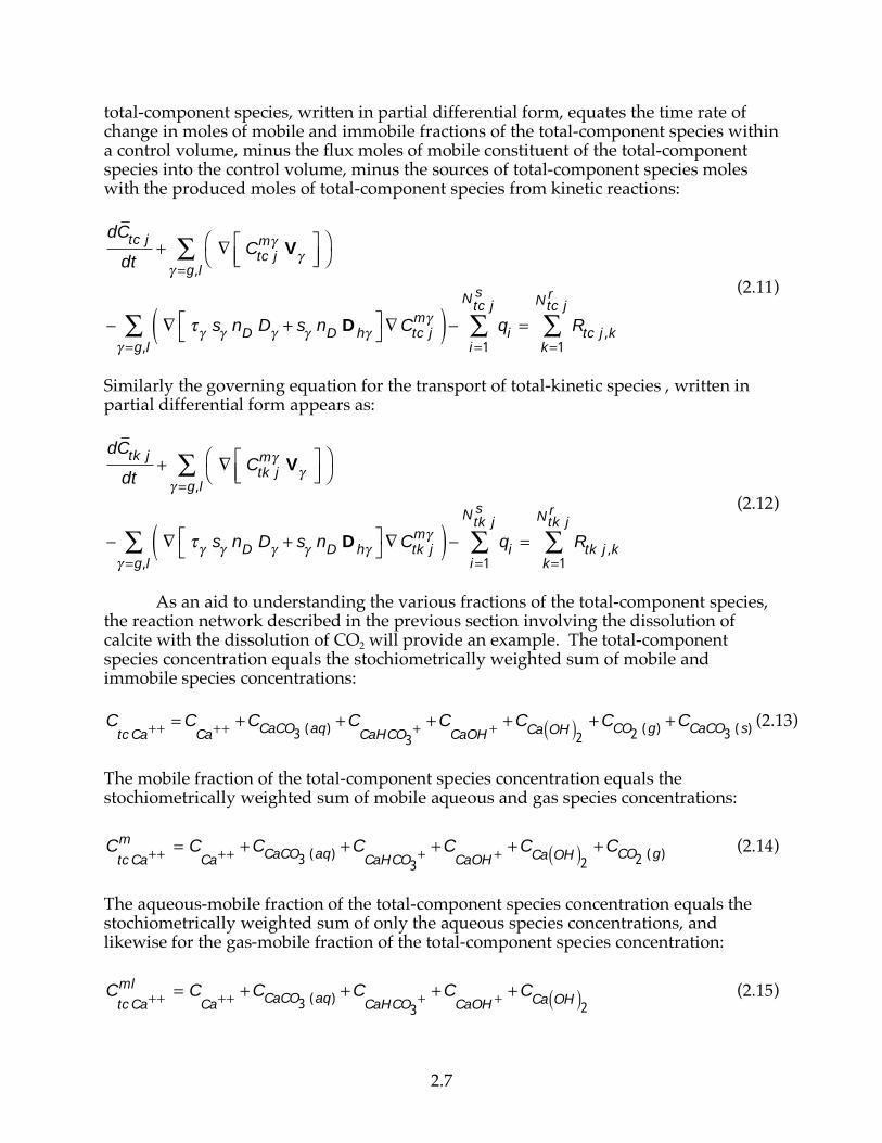
total-component species, written in partial differential form, equates the time rate of change in moles of mobile and immobile fractions of the total-component species within a control volume, minus the flux moles of mobile constituent of the total-component species into the control volume, minus the sources of total-component species moles with the produced moles of total-component species from kinetic reactions:

dCtc j

dt+ C

tc j

mV

=g,l

s nD

D + s nD

Dh

Ctc j

m( )=g,l

qi

i=1

Ntc j

s

= Rtc j,k

k=1

Ntc jr

(2.11)

Similarly the governing equation for the transport of total-kinetic species , written in partial differential form appears as:

dCtk j

dt+ C

tk j

mV

=g,l

s nD

D + s nD

Dh

Ctk j

m( )=g,l

qi

i=1

Ntk j

s

= Rtk j,k

k=1

Ntk jr

(2.12)

As an aid to understanding the various fractions of the total-component species, the reaction network described in the previous section involving the dissolution of calcite with the dissolution of CO2 will provide an example. The total-component species concentration equals the stochiometrically weighted sum of mobile and immobile species concentrations:

Ctc Ca

++= C

Ca++

+CCaCO3 (aq)

+CCaHCO3

++C

CaOH++C

Ca OH( )2

+CCO2 (g)

+CCaCO3 (s)

(2.13)

The mobile fraction of the total-component species concentration equals the stochiometrically weighted sum of mobile aqueous and gas species concentrations:

Ctc Ca

++m = C

Ca++

+CCaCO3 (aq)

+CCaHCO3

++C

CaOH++C

Ca OH( )2

+CCO2 (g)

(2.14)

The aqueous-mobile fraction of the total-component species concentration equals the stochiometrically weighted sum of only the aqueous species concentrations, and likewise for the gas-mobile fraction of the total-component species concentration:

Ctc Ca

++ml = C

Ca++

+CCaCO3 (aq)

+CCaHCO3

++C

CaOH++C

Ca OH( )2

(2.15)

2.8

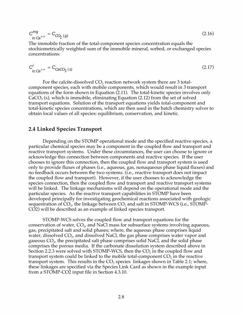
Ctc Ca

++

mg = C

CO2 (g) (2.16)

The immobile fraction of the total-component species concentration equals the stochiometrically weighted sum of the immobile mineral, sorbed, or exchanged species concentrations:

Ctc Ca

++

i = CCaCO3 (s)

(2.17)

For the calcite-dissolved CO2 reaction network system there are 3 total-component species, each with mobile components, which would result in 3 transport equations of the form shown in Equation (2.11). The total-kinetic species involves only CaCO3 (s), which is immobile, eliminating Equation (2.12) from the set of solved transport equations. Solution of the transport equations yields total-component and total-kinetic species concentrations, which are then used in the batch chemistry solver to obtain local values of all species: equilibrium, conservation, and kinetic.

2.4 Linked Species Transport Depending on the STOMP operational mode and the specified reactive species, a particular chemical species may be a component in the coupled flow and transport and reactive transport systems. Under these circumstances, the user can choose to ignore or acknowledge this connection between components and reactive species. If the user chooses to ignore this connection, then the coupled flow and transport system is used only to provide fluxes of phases (i.e., aqueous, gas, nonaqueous phase liquid fluxes) and no feedback occurs between the two systems. (i.e., reactive transport does not impact the coupled flow and transport). However, if the user chooses to acknowledge the species connection, then the coupled flow and transport and reactive transport systems will be linked. The linkage mechanisms will depend on the operational mode and the particular species. As the reactive transport capabilities in STOMP have been developed principally for investigating geochemical reactions associated with geologic sequestration of CO2, the linkage between CO2 and salt in STOMP-WCS (i.e., STOMP-CO2) will be described as an example of linked species transport. STOMP-WCS solves the coupled flow and transport equations for the conservation of water, CO2, and NaCl mass for subsurface systems involving aqueous, gas, precipitated salt and solid phases; where, the aqueous phase comprises liquid water, dissolved CO2, and dissolved NaCl, the gas phase comprises water vapor and gaseous CO2, the precipitated salt phase comprises solid NaCl, and the solid phase comprises the porous media. If the carbonate dissolution system described above in Section 2.2.3 were solved with STOMP-WCS, then the CO2 in the coupled flow and transport system could be linked to the mobile total-component CO2 in the reactive transport system. This results in the CO2 species linkages shown in Table 2.1; where, these linkages are specified via the Species Link Card as shown in the example input from a STOMP-CO2 input file in Section 4.3.10.

2.9

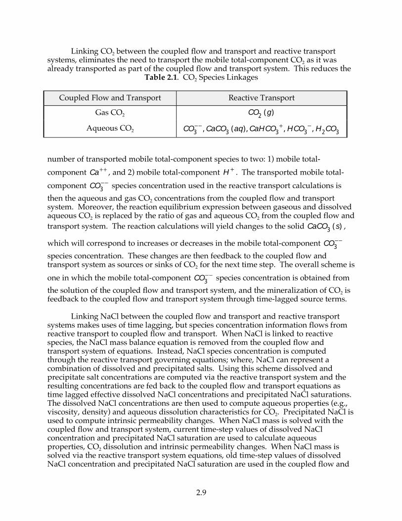
Linking CO2 between the coupled flow and transport and reactive transport systems, eliminates the need to transport the mobile total-component CO2 as it was already transported as part of the coupled flow and transport system. This reduces the

Table 2.1. CO2 Species Linkages

Coupled Flow and Transport Reactive Transport

Gas CO2 CO

2(g)

Aqueous CO2 CO

3, CaCO

3(aq), CaHCO

3+ , HCO

3, H

2CO

3

number of transported mobile total-component species to two: 1) mobile total-

component Ca++ , and 2) mobile total-component H

+ . The transported mobile total-

component CO

3 species concentration used in the reactive transport calculations is

then the aqueous and gas CO2 concentrations from the coupled flow and transport system. Moreover, the reaction equilibrium expression between gaseous and dissolved aqueous CO2 is replaced by the ratio of gas and aqueous CO2 from the coupled flow and transport system. The reaction calculations will yield changes to the solid

CaCO

3(s) ,

which will correspond to increases or decreases in the mobile total-component CO

3

species concentration. These changes are then feedback to the coupled flow and transport system as sources or sinks of CO2 for the next time step. The overall scheme is

one in which the mobile total-component CO

3 species concentration is obtained from

the solution of the coupled flow and transport system, and the mineralization of CO2 is feedback to the coupled flow and transport system through time-lagged source terms. Linking NaCl between the coupled flow and transport and reactive transport systems makes uses of time lagging, but species concentration information flows from reactive transport to coupled flow and transport. When NaCl is linked to reactive species, the NaCl mass balance equation is removed from the coupled flow and transport system of equations. Instead, NaCl species concentration is computed through the reactive transport governing equations; where, NaCl can represent a combination of dissolved and precipitated salts. Using this scheme dissolved and precipitate salt concentrations are computed via the reactive transport system and the resulting concentrations are fed back to the coupled flow and transport equations as time lagged effective dissolved NaCl concentrations and precipitated NaCl saturations. The dissolved NaCl concentrations are then used to compute aqueous properties (e.g., viscosity, density) and aqueous dissolution characteristics for CO2. Precipitated NaCl is used to compute intrinsic permeability changes. When NaCl mass is solved with the coupled flow and transport system, current time-step values of dissolved NaCl concentration and precipitated NaCl saturation are used to calculate aqueous properties, CO2 dissolution and intrinsic permeability changes. When NaCl mass is solved via the reactive transport system equations, old time-step values of dissolved NaCl concentration and precipitated NaCl saturation are used in the coupled flow and

2.10

transport calculations. Using old time-step values of NaCl decreases the accuracy of the solution, but increases the computational speed and numerical stability.

3.1

3.0 Numerical Solution

3.1 Introduction Two types of approaches are popular for solving reactive transport problems in multifluid geologic media: 1) direct substitution and 2) operator splitting (Yeh and Tripathi 1989; Yeh and Tripathi 1991; Steefel and Yabusaki 1996; Xu et al. 1997). The direct substitution approach involves substituting the reaction equations into the transport equations and solving them simultaneously, using a nonlinear equation solution approach (generally Newton-Raphson). This approach yields a direct solution of the species concentration and is considered to be more robust than the operator splitting approaches. Within the operator spliting approaches, there are two schemes: 1) sequential iteration and 2) non-sequential iteration. The sequential iteration solves the transport and batch chemistry governing equations sequentially, using Picard iteration (i.e., successive substitution) until convergence on the species concentration is reached. Yeh and Tripathi (1989) compared the direct substitution approach against the sequential iteration approach and concluded that computationally the sequential iteration approach was preferred for sufficiently large grids. More recently Saaltink et al. (2001) compared the two approaches in terms of computational domain and quality of solution for varying grid sizes. They concluded that the direct substitution method was more computationally efficient for smaller grid systems, especially when the chemical reactions were highly nonlinear or included significant retardation, but noted that the computational advantages diminished or reversed as the grid size increased. The reactive transport capabilities of the ECKEChem module, developed for the STOMP simulator have been aimed at field-scale applications involving large computational domains and complex multifluid nonisothermal coupled flow and transport systems. The computational demands of these types of simulations are significant, even without including the reactive transport component. Because of the simulation objectives and intended applications, only the operator split numerical solution method has been implemented for reactive transport in the STOMP simulator.

3.2 Species Transport

The operator splitting approach involves sequentially solving the species transport and batch chemistry, with species transport being first in the sequence. For equilibrium or mixed equilibrium and kinetic reaction systems, the number of transported species can be reduced, increasing computational efficiency, by transporting only the mobile total-component and total-kinetic species (Steefel and Yabusaki 1996; Xu et al. 1997). The governing equations for species transport of mobile total-component and total-kinetic species (Equations 2.11 and 2.12) are discretized temporially using a backward-Euler time differencing (fully implicit) and spatially using the integral finite difference method (White and Oostrom 2000) applied to structured orthogonal grid systems with a seven-point stencil.

3.2

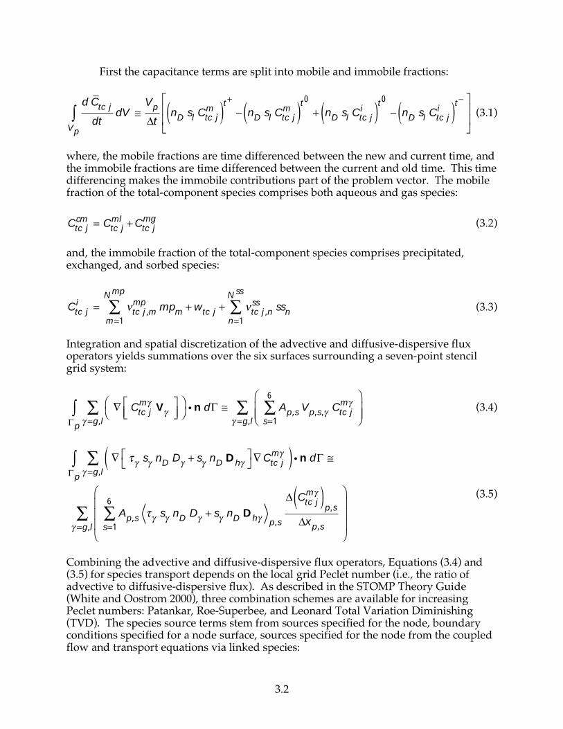
First the capacitance terms are split into mobile and immobile fractions:

d Ctc j

dtdV

Vp

V

p

tn

Ds

lC

tc j

m( )t+

nD

sl

Ctc j

m( )t0

+ nD

sl

Ctc j

i( )t0

nD

sl

Ctc j

i( )t

(3.1)

where, the mobile fractions are time differenced between the new and current time, and the immobile fractions are time differenced between the current and old time. This time differencing makes the immobile contributions part of the problem vector. The mobile fraction of the total-component species comprises both aqueous and gas species:

C

tc j

cm = Ctc j

ml+C

tc j

mg (3.2)

and, the immobile fraction of the total-component species comprises precipitated, exchanged, and sorbed species:

Ctc j

i = tc j,mmp

mpm

m=1

Nmp

+ wtc j

+tc j,nss

ssn

n=1

Nss

(3.3)

Integration and spatial discretization of the advective and diffusive-dispersive flux operators yields summations over the six surfaces surrounding a seven-point stencil grid system:

Ctc j

mV

=g,lp

i n d Ap,s

Vp,s,

Ctc j

m

s=1

6

=g,l

(3.4)

s nD

D + s nD

Dh

Ctc j

m( )=g,l

p

i n d

Ap,s

s nD

D + s nD

Dh

p,s

Ctc j

m( )p,s

xp,ss=1

6

=g,l

(3.5)

Combining the advective and diffusive-dispersive flux operators, Equations (3.4) and (3.5) for species transport depends on the local grid Peclet number (i.e., the ratio of advective to diffusive-dispersive flux). As described in the STOMP Theory Guide (White and Oostrom 2000), three combination schemes are available for increasing Peclet numbers: Patankar, Roe-Superbee, and Leonard Total Variation Diminishing (TVD). The species source terms stem from sources specified for the node, boundary conditions specified for a node surface, sources specified for the node from the coupled flow and transport equations via linked species:

3.3

qi

i=1

Ntc j

s

dV

Vp

Vp

qi

source+q

i

boundary+q

i

coupled flow( )i=1

Ntc j

s

(3.6)

Kinetic reactions are computed based on the nodal species concentrations at the current time step, which makes these terms part of the problem vector

Rtc j,k

k=1

Ntc jr

dV

Vp

Vp

Rtc j,k( )

t0

k=1

Ntc jr

(3.7)

Temporal and spatial discretization of the total-kinetic species transport equations follows that for total-component species.

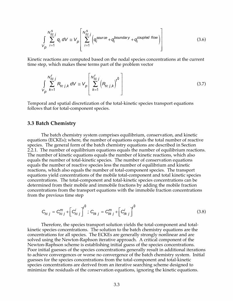
3.3 Batch Chemistry The batch chemistry system comprises equilibrium, conservation, and kinetic equations (ECKEs); where, the number of equations equals the total number of reactive species. The general form of the batch chemistry equations are described in Section 2.2.1. The number of equilibrium equations equals the number of equilibrium reactions. The number of kinetic equations equals the number of kinetic reactions, which also equals the number of total-kinetic species. The number of conservation equations equals the number of reactive species less the number of equilibrium and kinetic reactions, which also equals the number of total-component species. The transport equations yield concentrations of the mobile total-component and total kinetic species concentrations. The total-component and total-kinetic species concentrations can be determined from their mobile and immobile fractions by adding the mobile fraction concentrations from the transport equations with the immobile fraction concentrations from the previous time step

C

tc j = C

tc j

m+ C

tc j

it0

; Ctk j

= Ctk j

m+ C

tk j

it0

(3.8)

Therefore, the species transport solution yields the total-component and total-kinetic species concentrations. The solution to the batch chemistry equations are the concentrations for all species. The ECKEs are generally strongly nonlinear and are solved using the Newton-Raphson iterative approach. A critical component of the Newton-Raphson scheme is establishing initial guess of the species concentrations. Poor initial guesses of the species concentrations generally result in additional iterations to achieve convergences or worse no convergence of the batch chemistry system. Initial guesses for the species concentrations from the total-component and total-kinetic species concentrations are derived from an iterative searching scheme designed to minimize the residuals of the conservation equations, ignoring the kinetic equations.

3.4

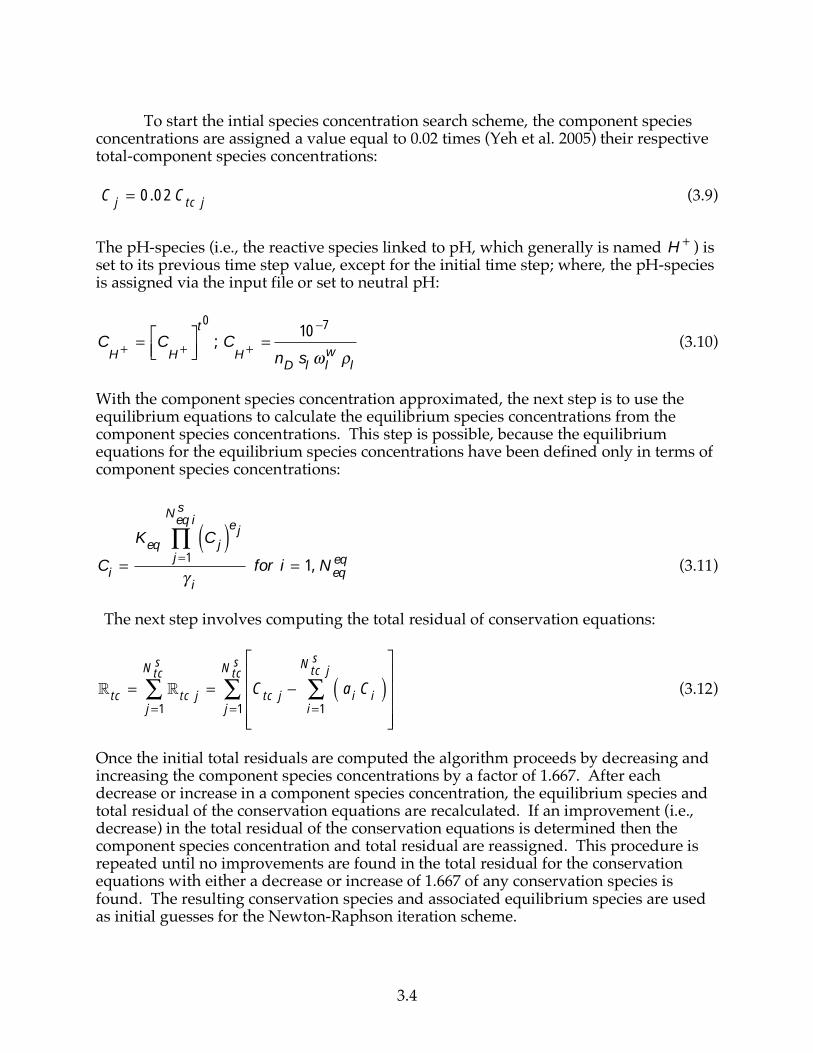
To start the intial species concentration search scheme, the component species concentrations are assigned a value equal to 0.02 times (Yeh et al. 2005) their respective total-component species concentrations: C

j = 0.02 C

tc j (3.9)

The pH-species (i.e., the reactive species linked to pH, which generally is named H+ ) is

set to its previous time step value, except for the initial time step; where, the pH-species is assigned via the input file or set to neutral pH:

CH+

= CH+

t0

; CH+

=10 7

nD

sl l

w

l

(3.10)

With the component species concentration approximated, the next step is to use the equilibrium equations to calculate the equilibrium species concentrations from the component species concentrations. This step is possible, because the equilibrium equations for the equilibrium species concentrations have been defined only in terms of component species concentrations:

Ci =

Keq

Cj( )

ej

j=1

Neq i

s

i

for i = 1, Neq

eq (3.11)

The next step involves computing the total residual of conservation equations:

tc =

tc j

j=1

Ntcs

= Ctc j

ai

Ci( )

i=1

Ntc j

s

j=1

Ntcs

(3.12)

Once the initial total residuals are computed the algorithm proceeds by decreasing and increasing the component species concentrations by a factor of 1.667. After each decrease or increase in a component species concentration, the equilibrium species and total residual of the conservation equations are recalculated. If an improvement (i.e., decrease) in the total residual of the conservation equations is determined then the component species concentration and total residual are reassigned. This procedure is repeated until no improvements are found in the total residual for the conservation equations with either a decrease or increase of 1.667 of any conservation species is found. The resulting conservation species and associated equilibrium species are used as initial guesses for the Newton-Raphson iteration scheme.

3.5

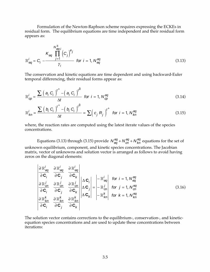
Formulation of the Newton-Raphson scheme requires expressing the ECKEs in residual form. The equilibrium equations are time independent and their residual form appears as:

eq

i= C

i

Keq

Cj( )

ej

j=1

Neq i

s

i

for i = 1, Neq

eq (3.13)

The conservation and kinetic equations are time dependent and using backward-Euler temporal differencing, their residual forms appear as:

cp

i=

ai

Ci( )

t+

ai

Ci( )

t0

t for i = 1, N

cp

eq (3.14)

kn

i=

bi

Ci( )

t+

bi

Ci( )

t0

t = c

jR

j( )t+

for i = 1, Nkn

eq (3.15)

where, the reaction rates are computed using the latest iterate values of the species concentrations.

Equations (3.13) through (3.15) provide N

eq

eq+ N

cn

eq+ N

kn

eq equations for the set of

unknown equilibrium, component, and kinetic species concentrations. The Jacobian matrix, vector of unknowns and solution vector is arranged as follows to avoid having zeros on the diagonal elements:

eq

i

Ci

eq

i

Cj

eq

i

Ck

cn

j

Ci

cn

j

Cj

cn

j

Ck

kn

k

Ci

kn

k

Cj

kn

k

Ck

Ci

Cj

Ck

=

eq

i

cn

j

kn

k

for i = 1, Neq

eq

for j = 1, Ncn

eq

for k = 1, Nkn

eq

(3.16)

The solution vector contains corrections to the equilibrium-, conservation-, and kinetic-equation species concentrations and are used to update these concentrations between iterations:

3.6

s+1C

i = s

Ci+ C

i for i = 1, N

eq

eq

s+1C

j = s

Cj+ C

j for j = 1, N

cn

eq

s+1C

k = s

Ck+ C

k for k = 1, N

kn

eq

(3.17)

where, superscript s indicates the current iterate level and superscript s+1 indicates the next iterate level. The system of equations is considered converged when the maximum relative residual or change in concentration falls below a specified tolerance level. To avoid negative concentrations of the species the change in species concentration is restricted. In the Newton-Raphson iteration scheme, the species concentrations are the primary variables. For the Newton-Raphson scheme to execute properly the equation residual must have a dependence on the primary variable (i.e., species concentration) selected for that equation. The primary unknowns for the equilibrium equations are equilibrium species, and for the conservation equations are the component species. For the equilibrium and conseration equation there is a direct correspondence between equations and primary unknowns. For the kinetic equations, however, the primary unknown species must be chosen such that equation residuals are strongly dependent on the species concentration. An equation sequencing algorithm is used to correlate species concentrations with chemistry equations.

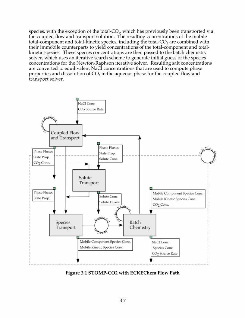
3.4 Algorithm Structure and Flow Path Reactive transport capabilities of the ECKEChem module have been designed to work with all operational modes of the STOMP simulator, without significantly altering the STOMP coding. This section describes the algorithm structure, the modular coding, and the flow path for solving multifluid subsurface flow and reactive transport problems with the STOMP simulator and ECKEChem module. The core capabilities of the STOMP simulator, prior to developing the ECKEChem module, included coupled multifluid subsurface flow and transport and solute transport; where, the two systems are solved sequentially. As the numerical solution approach for the reactive transport system uses an operator splitting scheme, which sequentially computes species transport and batch chemistry, the solute transport schemes of the STOMP simulator can be used for transporting reactive species with only minor modifcations. The flow path for the coupled STOMP-CO2 and ECKEChem module are shown in Figure 3.1. A time step begins with the solution of the coupled flow and transport system, using Newton Raphson iteration, yielding aqueous and gas phase fluxes, state properties (e.g., temperature, pressure, phase viscosity, phase density, phase saturation), and the concentrations of gaseous and aqueous dissolved CO2. If transport of nonreactive dilute solutes is specified for the simulation, then solute transport is computed, with the option for sub-time stepping as a function of the maximum Courant number. Inputs to the solute transport solver include aqueous and gas phase fluxes, state properties, and the previous time-step or sub-time-step solute concentrations. Multiple solutes are transported sequentially. Using the operator splitting scheme, the reactive transport solution begins with transport of all the mobile total-component and total-kinetic

3.7

species, with the exception of the total-CO2, which has previously been transported via the coupled flow and transport solution. The resulting concentrations of the mobile total-component and total-kinetic species, including the total-CO2 are combined with their immobile counterparts to yield concentrations of the total-component and total-kinetic species. These species concentrations are then passed to the batch chemistry solver, which uses an iterative search scheme to generate initial guess of the species concentrations for the Newton-Raphson iterative solver. Resulting salt concentrations are converted to equilivalent NaCl concentrations that are used to compute phase properties and dissolution of CO2 in the aqueous phase for the coupled flow and transport solver.

Figure 3.1 STOMP-CO2 with ECKEChem Flow Path

4.1

4.0 Input File

4.1 Introduction Inputs required to execute the reactive transport routines in the STOMP simulator are specified through cards in the “input” file; where, the word card refers to an associated group of inputs. This addendum provides a brief description and formatting details for each of the reactive transport input cards and modifications to the Solution Control Card, Boundary Condition Card, Initial Condition Card, and Output Control Card. Descriptions and formatting details for other STOMP input cards are provided in the STOMP User’s Guide (White and Oostrom, 2004). To distinguish between the solute transport and first-order chemical reaction capabilities of STOMP that existed in the code prior to the inclusion of reactive transport, the term species will refer to reactive species and the term solute will refer to the original solute transport and reaction capabilities. The reactive transport modules have been incorporated into STOMP independently from the solute transport algorithms, allowing the user to specify both solute and reactive-species transport in a single simulation.

4.2 Card Descriptions Formatting instructions for the input cards are provided in Section 4.3. This section provides a brief synopsis of each input card with emphasis on its purpose and application. Italicized words refer to specific files, cards, options and data entries shown in the card formats in Section 4.3. For easy reference, input cards are listed in alphabetical order in Section 4.3. In this section, input cards are listed in a sequence most user’s find convenient when developing an input file.

4.2.1 Aqueous Species Card This card defines the aqueous species to be considered in the simulation. Required input includes the species name, aqueous molecular diffusion coefficient for all species, activity coefficient model option, species charge, species diameter, and species molecular weight. The species name must be unique and distinct from gas and solid species names (e.g., CO2(aq), CO2_aqueous, dissolved CO2, CO2a). Because only component and kinetic species are transport, transport properties, such as diffusion coefficients, are species independent. Currently, the activity coefficient models include Davies, B-Dot, Pitzer and a constant coefficient option. If the constant coefficient option is chosen then the species charge, diameter, molecular weight inputs are not required.

4.2.2 Gas Species Card This card defines the gas species to be considered in the simulation. Required input includes the species name, gas molecular diffusion coefficient for all species, associate aqueous species name, and gas-aqueous partitioning parameters. The species

4.2

name must be unique and distinct from aqueous and solid species names (e.g., CO2(g), CO2_gas, gaseous CO2, CO2g). All gas species must be associated with an aqueous species, with which it is in equilibrium. Equilibrium partitioning between the gas and aqueous species is specified via a temperature dependent function, whose parameters are entered on this card.

4.2.3 Solid Species Card This card defines the solid species to be considered in the simulation. Required input includes the species name, species mass density, and species molecular weight. The species name must be unique and distinct from aqueous and gas species names (e.g., FeCO3(s), FeCO3_solid, solid FeCO3, FeCO3s).

4.2.4 Lithology Card This card specifies the mineral specific areas and species volume fractions for every rock/soil type defined on the Rock/Soil Zonation Card. This card is only required when specific kinetic reactions types are specified on the Kinetic Reactions Card. Currently this card is only required when the Precipitation-Dissolution kinetic reaction type is specified for the Kinetic Reaction Type option. Required input for each rock/soil type includes the primary and secondary mineral specific area, and species volume fractions for every solid species defined on the Solid Species Card.

4.2.5 Equilibrium Reactions Card This card specifies the equilibrium reaction constants to be considered in the simulation. Species are associated with the defined equilibrium reaction constants via the Equilibrium Equations Card. This card is only used to specify the parameters used in the temperature dependent equations for equilibrium constants, as shown in Equation (2.x). Required inputs include the equilibrium reaction name and equation coefficients for the temperature dependent equilibrium constant. The equilibrium reaction name must be unique and distinct from kinetic reaction names (e.g., EqRc-1, E1, Equil-Reac-1, er-1).

4.2.6 Kinetic Reactions Card This card specifies the kinetic reactions to be considered in the simulation. Required inputs include the kinetic reaction name, kinetic reaction type, number of reactant species, reactant species names, reactant species stochiometric coefficients, number of product species, product species names, product species stochiometric coefficients, and kinetic reaction parameters. The kinetic reaction name must be unique and distinct from equilibrium reaction names (e.g., KnRc-1, K1, Kin-Reac-1, kr-1). The required kinetic reaction parameters depends on the specified Kinetic Reaction Type option. For the Precipitation-Dissolution kinetic reaction type (Equation (2.x)), the required reaction parameters include the reference forward and backward reaction rates, reaction activation energy, reference temperature, and equation coefficients for the temperature dependent equilibrium constant, as shown in Equation (2.x).

4.3

For the Forward-Backward kinetic reaction type (Equation (2.x)), the required reaction parameters include the forward and backward rate exponents. For the Valocchi-Monod kinetic reaction type (Equation (2.x)), the required reaction parameters include the acceptor half-saturation constant, maximum specific rate of substrate utilization, microbial yield coefficient, and first-order microbial decay coefficient. For the Valocchi-Sorption kinetic reaction type (Equation (2.x)), the required reaction parameters include the mass transfer and distribution coefficients.

4.2.7 Equilibrium Equations Card This card specifies the equilibrium equations to be considered in the simulation. Equilibrium equations have the following general form:

Ci( ) = K

eqC

j( )e

j

j i

(4.1)

where, K

eq is an equilibrium reaction constant specified via the Equilibirum Reactions

Card, C

i( ) is the activity of the equilibrium species i, and C

j( ) is the activity of the

species j in the equilibrium equation. Activity coefficients and model options are specified via the Aqueous Species Card. The species exponents

e

j can be positive or

negative. Required inputs include the number of species in the equilibrium equation (including the equilibrium species), species names, equilibrium reaction name, and the species exponents. The equilibrium species (indicated with the subscript i ) is distinguished from the other species in the equilibrium equation (indicated with the subscript j ) by being the first species listed for the equilibrium equation.

4.2.8 Conservation Equations Card This card specifies the conservation equations to be considered in the simulation. Conservation equations have the following general form:

d ai

Ci( )

dt = 0 (4.2)

where,

C

i is the concentration of species i (expressed as aqueous molar concentration),

and a

i is the stochiometric coefficient of species i, and

a

iC

i( ) is the component species concentration (expressed as aqueous molar concentration). Required inputs include the component species name, number of species in the conservation equation, species names, and species stochiometric coefficients. The component species name must begin with “Total_” followed with the species name of a reactive species in the conservation equation (e.g., Total_CO2, Total_H2CO3, Total_H+). This name specification is critical in that it links the named species with the conservation equation,

4.4

making the concentration for that species the primary unknown for the conservation equation.

4.2.9 Kinetic Equations Card This card specifies the kinetic equations to be considered in the simulation. Kinetic equations have the following general form:

d bi

Ci( )

dt = c

jR

j( ) (4.3)

where,

C

i is the concentration of species i (expressed as aqueous molar concentration),

and b

i is the stochiometric coefficient of species i,

b

iC

i( ) is the kinetic species

concentration (expressed as aqueous molar concentration), R

j is the kinetic-reaction

rate, and c

j is the kinetic-reaction-rate coefficient. Required inputs include the number

of species, species names, species stochiometric coefficients, number of kinetic-reaction rates, kinetic reaction names, and kinetic-reaction-rate coefficients. Kinetic-reaction names and associated rate functions are defined on the Kinetic Reactions Card.

4.2.10 Species Link Card This card associates reactive species with components in the coupled flow and transport equations and defines which species name defines the system pH. Currently the following coupled flow and transport components can be associated: aqueous water, gas water, aqueous air, gas air, aqueous CO2, gas CO2, aqueous CH4, gas CH4, aqueous salt, and solid salt. Required inputs include the number of reactive species links, species names, and linked components (i.e., Aqueous pH, Aqueous Water, Gas Water, Aqueous Air, Gas Air, Aqueous CO2, Gas CO2, Aqueous CH4, and Gas CH4).

4.2.11 Initial Conditions Card This card has been modified to allow for reactive species concentrations to be initialized. Initial aqueous or solid species concentrations can be entered as node volume molar, aqueous molar or aqueous molal. Initial gas species concentrations can be entered as node volume molar, gas molar, aqueous molar or aqueous molal. Required inputs are the species name, concentration type specification, concentration value, concentration units, concentration gradients, and domain region. To distinguish reactive species and transported solutes, the keyword Species needs to be included in the concentration type specification (e.g., Species Aqueous Volumetric Concentration, Species Aqueous Molal ). Formatting requirements for specifying initial species concentrations are identical to those for specifying initial solute concentrations.

4.5

Internally all species concentrations, including gas and solid species are stored as aqueous molar concentrations (i.e., mole/m3

aqueous).

4.2.12 Boundary Conditions Card This card has been modified to allow for boundary conditions to be specified for reactive species. Chemical reaction system generally involve large numbers of reactive species, which has necessitated some formatting changes for this card. Reactive species boundary condition types include: Aqueous Concentration, Inflow Aqueous, Outflow Aqueous, Inflow-Outflow Aqueous Concentration, Zero-Flux, and Initial Condition. Equilibrium conditions are assumed between gas and aqueous species. The three principal departures from the conventional formatting for the Boundary Conditions Card are 1) a single boundary condition type is applied to all reactive species, 2) not all reactive species concentrations need to be specified, and 3) line returns are permitted to allow for large numbers of reactive species. Required inputs, specific to the reactive species, include the boundary condition type, and then at each time point the number of species, species name, species concentration, and species concentration units. Line returns are allowed during the specification of boundary condition values at each time point. Although individual species concentration are specified on the boundaries, these concentrations are converted to component and kinetic species before being transported across the boundary surface.

4.2.13 Source Card This card has been modified to allow for sources to be specified for reactive species. Reactive species sources are specified in the same manner as solute sources, using a species rate (i.e., mol/s) or species density rate (i.e., mol/m3

grid volume s). Required input includes the source type, species name, source domain, the number of time points, and for each time point the time, and species source rate and units.

4.2.14 Output Control Card This card has been modified to allow for reactive species output to the output and plot.n files. Reactive species output in Reference Node or Plot File forms is specified in the same manner as solute output, with the exception that the keyword Species is used instead of Solute. Required input includes the output variable, species name, and output units.

4.2.15 Surface Flux Card This card has been modified to allow for reactive species surface flux output to the surface file. Reactive species surface flux output is specified in the same manner as solute surface flux output, with the exception that the keyword Species is used instead of Solute. Required input includes the surface flux type, species name, and surface flux rate and integral units, surface direction, and surface domain.

4.6

4.3 Input Card Formats Formatting instructions for STOMP input cards specific to reactive species are provided in this section. Explanations of the input format notation are provided in Appendix A of the STOMP User’s Guide (White and Oostrom 2004), and general formatting instructions for STOMP input cards are provided in Appendix B of the STOMP User’s Guide (White and Oostrom 2004).

4.3.1 Aqueous Species Card Card Titlea { ~Aqueous Species [ Card ] } Format: Chara, Number of Aqueous Speciesa, Aqueous Molecular Diffusion Coefficientb, Unitsc (m), [ Activity Coefficient Model Optiond, ] { Davies Equation | Pitzer Equation | Constant | B Dot } Format: Integera, Realb, Charc, [ Chard, ] For: Number of Aqueous Species Aqueous Species Namea, If: Activity Coefficient Model Option { Constant } Species Chargeb, Species Diameterc, Unitsd (m), Species Molecular Weighte, Unitsf (gm/mol), Format: Chara, Realb, Realc, Chard, Reale, Charf, Elseif: Activity Coefficient Model Option = { Constant } Species Activity Coefficientb,

Format: Chara, Realb, Endif: Endfor: Number of Aqueous Species Aqueous Species Card Examples: Extracted from a STOMP-WCS input file: ~Aqueous Species Card 10,1.e-9,cm^2/s,Constant Activity,1.0, Ca++,2.0,6.0,A,40.0780,kg/kmol, CO3--,-2.0,4.5,A,60.0092,kg/kmol, H+,1.0,9.0,A,1.0079,kg/kmol, OH-,-1.0,3.5,A,17.0073,kg/kmol, CaCO3(aq),0.0,3.0,A,100.0872,kg/kmol, CaHCO3+,1.0,4.0,A,101.0951,kg/kmol, CaOH+,1.0,4.0,A,57.0853,kg/kmol, HCO3-,-1.0,4.0,A,61.0171,kg/kmol, H2CO3,0.0,4.0,A,62.0250,kg/kmol, Ca(OH)2,0.0,4.0,A,74.0926,kg/kmol,

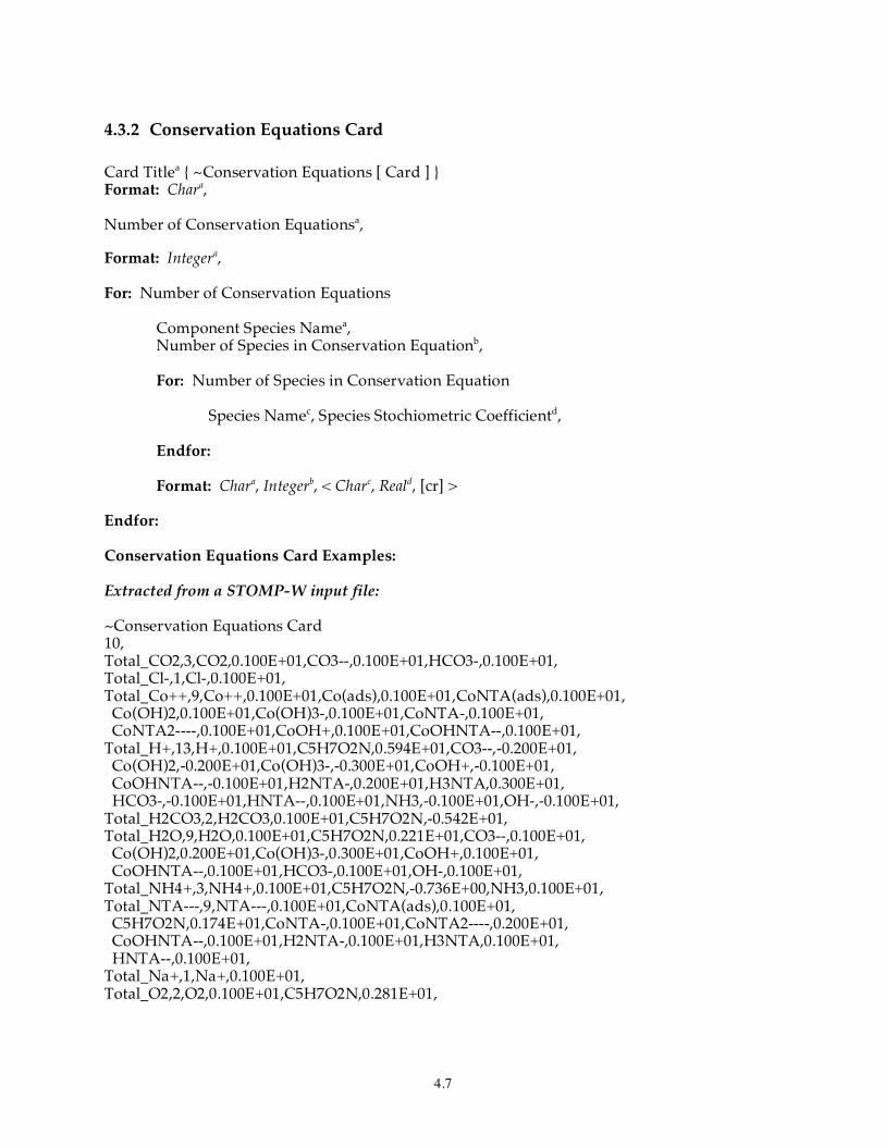
4.7

4.3.2 Conservation Equations Card Card Titlea { ~Conservation Equations [ Card ] } Format: Chara, Number of Conservation Equationsa, Format: Integera, For: Number of Conservation Equations Component Species Namea, Number of Species in Conservation Equationb, For: Number of Species in Conservation Equation Species Namec, Species Stochiometric Coefficientd, Endfor:

Format: Chara, Integerb, < Charc, Reald, [cr] >

Endfor: Conservation Equations Card Examples: Extracted from a STOMP-W input file: ~Conservation Equations Card 10, Total_CO2,3,CO2,0.100E+01,CO3--,0.100E+01,HCO3-,0.100E+01, Total_Cl-,1,Cl-,0.100E+01, Total_Co++,9,Co++,0.100E+01,Co(ads),0.100E+01,CoNTA(ads),0.100E+01, Co(OH)2,0.100E+01,Co(OH)3-,0.100E+01,CoNTA-,0.100E+01, CoNTA2----,0.100E+01,CoOH+,0.100E+01,CoOHNTA--,0.100E+01, Total_H+,13,H+,0.100E+01,C5H7O2N,0.594E+01,CO3--,-0.200E+01, Co(OH)2,-0.200E+01,Co(OH)3-,-0.300E+01,CoOH+,-0.100E+01, CoOHNTA--,-0.100E+01,H2NTA-,0.200E+01,H3NTA,0.300E+01, HCO3-,-0.100E+01,HNTA--,0.100E+01,NH3,-0.100E+01,OH-,-0.100E+01, Total_H2CO3,2,H2CO3,0.100E+01,C5H7O2N,-0.542E+01, Total_H2O,9,H2O,0.100E+01,C5H7O2N,0.221E+01,CO3--,0.100E+01, Co(OH)2,0.200E+01,Co(OH)3-,0.300E+01,CoOH+,0.100E+01, CoOHNTA--,0.100E+01,HCO3-,0.100E+01,OH-,0.100E+01, Total_NH4+,3,NH4+,0.100E+01,C5H7O2N,-0.736E+00,NH3,0.100E+01, Total_NTA---,9,NTA---,0.100E+01,CoNTA(ads),0.100E+01, C5H7O2N,0.174E+01,CoNTA-,0.100E+01,CoNTA2----,0.200E+01, CoOHNTA--,0.100E+01,H2NTA-,0.100E+01,H3NTA,0.100E+01, HNTA--,0.100E+01, Total_Na+,1,Na+,0.100E+01, Total_O2,2,O2,0.100E+01,C5H7O2N,0.281E+01,

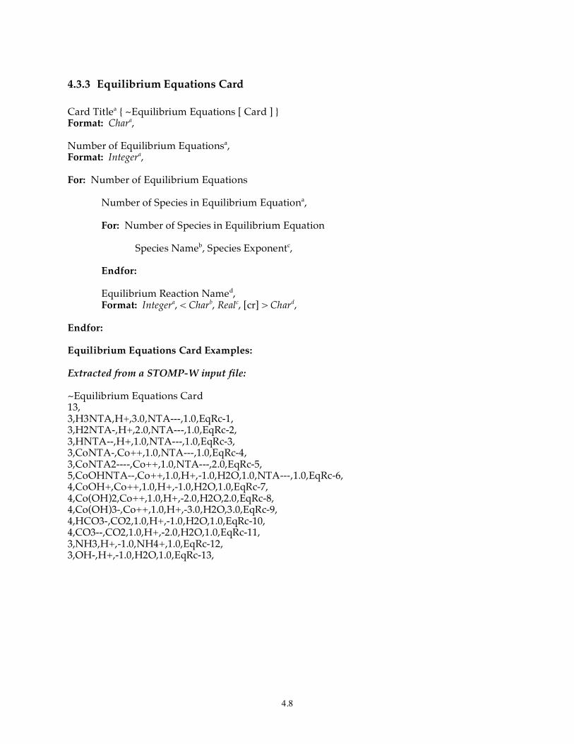
4.8

4.3.3 Equilibrium Equations Card Card Titlea { ~Equilibrium Equations [ Card ] } Format: Chara, Number of Equilibrium Equationsa, Format: Integera, For: Number of Equilibrium Equations Number of Species in Equilibrium Equationa, For: Number of Species in Equilibrium Equation Species Nameb, Species Exponentc, Endfor: Equilibrium Reaction Named,

Format: Integera, < Charb, Realc, [cr] > Chard,

Endfor: Equilibrium Equations Card Examples: Extracted from a STOMP-W input file: ~Equilibrium Equations Card 13, 3,H3NTA,H+,3.0,NTA---,1.0,EqRc-1, 3,H2NTA-,H+,2.0,NTA---,1.0,EqRc-2, 3,HNTA--,H+,1.0,NTA---,1.0,EqRc-3, 3,CoNTA-,Co++,1.0,NTA---,1.0,EqRc-4, 3,CoNTA2----,Co++,1.0,NTA---,2.0,EqRc-5, 5,CoOHNTA--,Co++,1.0,H+,-1.0,H2O,1.0,NTA---,1.0,EqRc-6, 4,CoOH+,Co++,1.0,H+,-1.0,H2O,1.0,EqRc-7, 4,Co(OH)2,Co++,1.0,H+,-2.0,H2O,2.0,EqRc-8, 4,Co(OH)3-,Co++,1.0,H+,-3.0,H2O,3.0,EqRc-9, 4,HCO3-,CO2,1.0,H+,-1.0,H2O,1.0,EqRc-10, 4,CO3--,CO2,1.0,H+,-2.0,H2O,1.0,EqRc-11, 3,NH3,H+,-1.0,NH4+,1.0,EqRc-12, 3,OH-,H+,-1.0,H2O,1.0,EqRc-13,

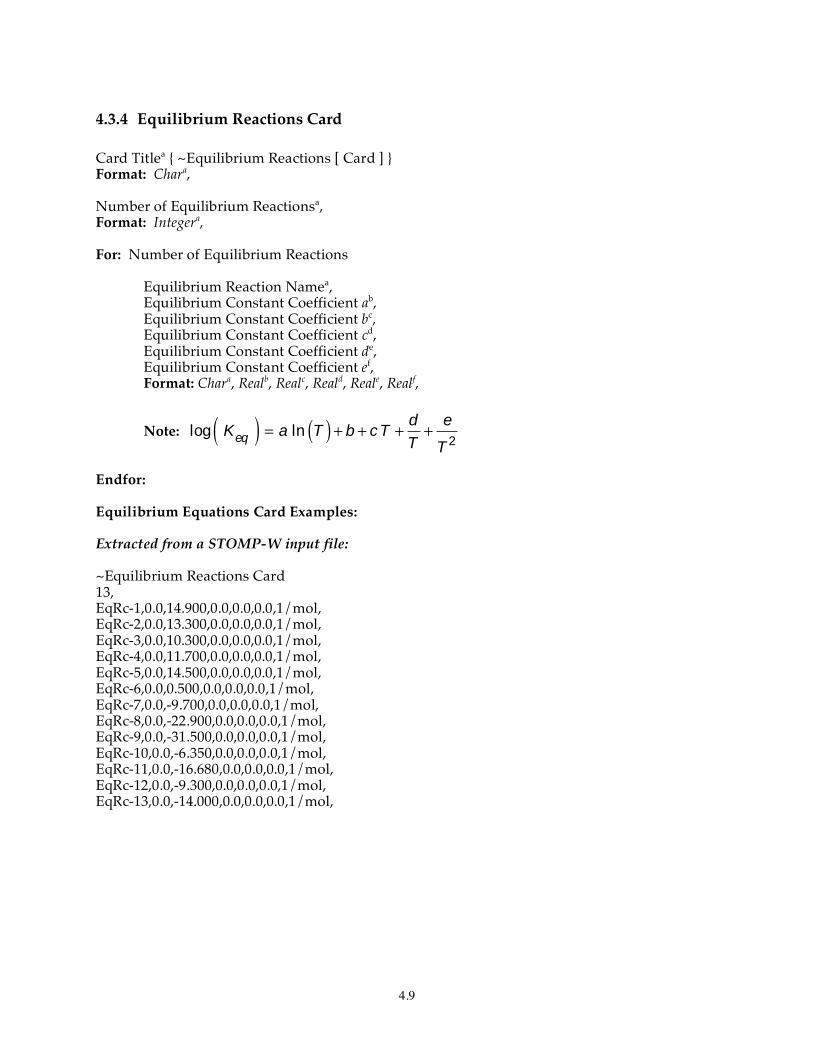
4.9

4.3.4 Equilibrium Reactions Card Card Titlea { ~Equilibrium Reactions [ Card ] } Format: Chara, Number of Equilibrium Reactionsa, Format: Integera, For: Number of Equilibrium Reactions Equilibrium Reaction Namea, Equilibrium Constant Coefficient ab, Equilibrium Constant Coefficient bc, Equilibrium Constant Coefficient cd, Equilibrium Constant Coefficient de, Equilibrium Constant Coefficient ef,

Format: Chara, Realb, Realc, Reald, Reale, Realf,

Note:

log Keq( ) = a ln T( ) + b + c T +

d

T+

e

T2

Endfor: Equilibrium Equations Card Examples: Extracted from a STOMP-W input file: ~Equilibrium Reactions Card 13, EqRc-1,0.0,14.900,0.0,0.0,0.0,1/mol, EqRc-2,0.0,13.300,0.0,0.0,0.0,1/mol, EqRc-3,0.0,10.300,0.0,0.0,0.0,1/mol, EqRc-4,0.0,11.700,0.0,0.0,0.0,1/mol, EqRc-5,0.0,14.500,0.0,0.0,0.0,1/mol, EqRc-6,0.0,0.500,0.0,0.0,0.0,1/mol, EqRc-7,0.0,-9.700,0.0,0.0,0.0,1/mol, EqRc-8,0.0,-22.900,0.0,0.0,0.0,1/mol, EqRc-9,0.0,-31.500,0.0,0.0,0.0,1/mol, EqRc-10,0.0,-6.350,0.0,0.0,0.0,1/mol, EqRc-11,0.0,-16.680,0.0,0.0,0.0,1/mol, EqRc-12,0.0,-9.300,0.0,0.0,0.0,1/mol, EqRc-13,0.0,-14.000,0.0,0.0,0.0,1/mol,

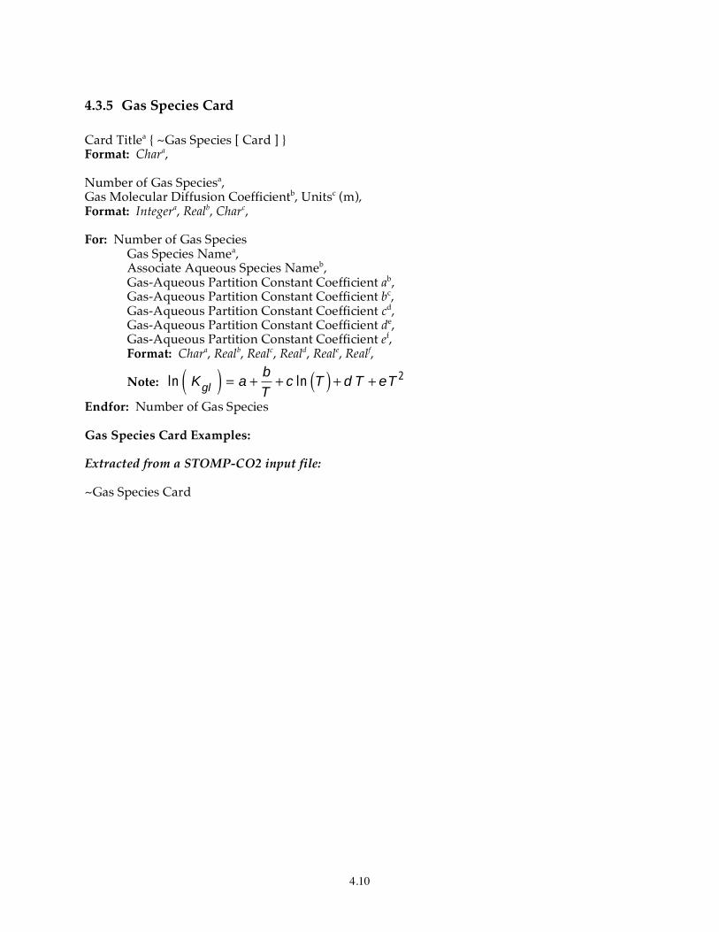
4.10

4.3.5 Gas Species Card Card Titlea { ~Gas Species [ Card ] } Format: Chara, Number of Gas Speciesa, Gas Molecular Diffusion Coefficientb, Unitsc (m), Format: Integera, Realb, Charc, For: Number of Gas Species Gas Species Namea, Associate Aqueous Species Nameb, Gas-Aqueous Partition Constant Coefficient ab, Gas-Aqueous Partition Constant Coefficient bc, Gas-Aqueous Partition Constant Coefficient cd, Gas-Aqueous Partition Constant Coefficient de, Gas-Aqueous Partition Constant Coefficient ef,

Format: Chara, Realb, Realc, Reald, Reale, Realf,

Note: ln K

gl( ) = a +b

T+ c ln T( ) + d T + e T

2

Endfor: Number of Gas Species Gas Species Card Examples: Extracted from a STOMP-CO2 input file: ~Gas Species Card

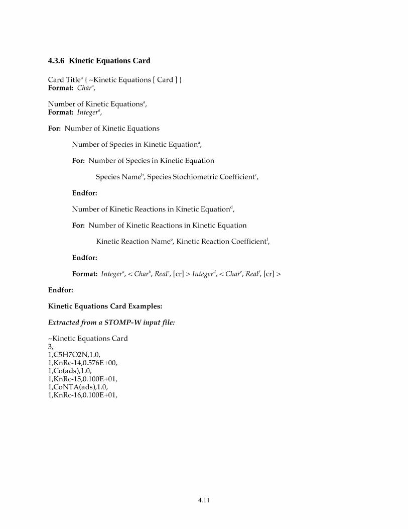
4.11

4.3.6 Kinetic Equations Card

Card Titlea { ~Kinetic Equations [ Card ] } Format: Chara, Number of Kinetic Equationsa, Format: Integera, For: Number of Kinetic Equations Number of Species in Kinetic Equationa, For: Number of Species in Kinetic Equation Species Nameb, Species Stochiometric Coefficientc, Endfor: Number of Kinetic Reactions in Kinetic Equationd, For: Number of Kinetic Reactions in Kinetic Equation Kinetic Reaction Namee, Kinetic Reaction Coefficientf, Endfor:

Format: Integera, < Charb, Realc, [cr] > Integerd, < Chare, Realf, [cr] >

Endfor: Kinetic Equations Card Examples: Extracted from a STOMP-W input file: ~Kinetic Equations Card 3, 1,C5H7O2N,1.0, 1,KnRc-14,0.576E+00, 1,Co(ads),1.0, 1,KnRc-15,0.100E+01, 1,CoNTA(ads),1.0, 1,KnRc-16,0.100E+01,

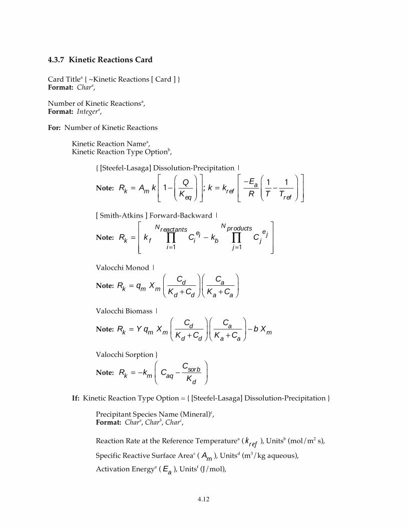
4.12

4.3.7 Kinetic Reactions Card Card Titlea { ~Kinetic Reactions [ Card ] } Format: Chara, Number of Kinetic Reactionsa, Format: Integera, For: Number of Kinetic Reactions Kinetic Reaction Namea, Kinetic Reaction Type Optionb, { [Steefel-Lasaga] Dissolution-Precipitation |

Note:

Rk

= Am

k 1Q

Keq

; k = kref

Ea

R

1

T

1

Tref

[ Smith-Atkins ] Forward-Backward |

Note:

Rk

= kf

Ci

ei

i=1

Nreactants

kb

Cj

ej

j=1

Nproducts

Valocchi Monod |

Note:

Rk

= qm

Xm

Cd

Kd+C

d

Ca

Ka+C

a

Valocchi Biomass |

Note:

Rk

= Y qm

Xm

Cd

Kd+C

d

Ca

Ka+C

a

b Xm

Valocchi Sorption }

Note:

Rk

= km

Caq

Csorb

Kd

If: Kinetic Reaction Type Option = { [Steefel-Lasaga] Dissolution-Precipitation }

Precipitant Species Name (Mineral)c, Format: Chara, Charb, Charc,

Reaction Rate at the Reference Temperaturea ( k

ref), Unitsb (mol/m2 s),

Specific Reactive Surface Areac ( A

m), Unitsd (m3/kg aqueous),

Activation Energye ( E

a), Unitsf (J/mol),

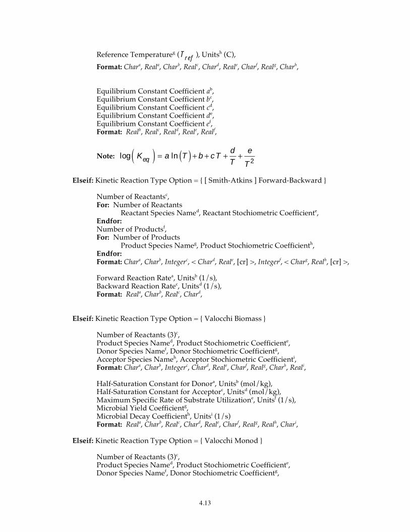
4.13

Reference Temperatureg ( T

ref), Unitsh (C),

Format: Chara, Reala, Charb, Realc, Chard, Reale, Charf, Realg, Charh,

Equilibrium Constant Coefficient ab, Equilibrium Constant Coefficient bc, Equilibrium Constant Coefficient cd, Equilibrium Constant Coefficient de, Equilibrium Constant Coefficient ef,

Format: Realb, Realc, Reald, Reale, Realf,

Note:

log Keq( ) = a ln T( ) + b + c T +

d

T+

e

T2

Elseif: Kinetic Reaction Type Option = { [ Smith-Atkins ] Forward-Backward } Number of Reactantsc, For: Number of Reactants Reactant Species Named, Reactant Stochiometric Coefficiente, Endfor: Number of Productsf, For: Number of Products Product Species Nameg, Product Stochiometric Coefficienth, Endfor: Format: Chara, Charb, Integerc, < Chard, Reale, [cr] >, Integerf, < Charg, Realh, [cr] >, Forward Reaction Ratea, Unitsb (1/s), Backward Reaction Ratec, Unitsd (1/s), Format: Reala, Charb, Realc, Chard, Elseif: Kinetic Reaction Type Option = { Valocchi Biomass } Number of Reactants (3)c, Product Species Named, Product Stochiometric Coefficiente,

Donor Species Namef, Donor Stochiometric Coefficientg, Acceptor Species Nameh, Acceptor Stochiometric Coefficienti,

Format: Chara, Charb, Integerc, Chard, Reale, Charf, Realg, Charh, Reali, Half-Saturation Constant for Donora, Unitsb (mol/kg), Half-Saturation Constant for Acceptorc, Unitsd (mol/kg), Maximum Specific Rate of Substrate Utilizatione, Unitsf (1/s), Microbial Yield Coefficientg, Microbial Decay Coefficienth, Unitsi (1/s) Format: Reala, Charb, Realc, Chard, Reale, Charf, Realg, Realh, Chari, Elseif: Kinetic Reaction Type Option = { Valocchi Monod } Number of Reactants (3)c, Product Species Named, Product Stochiometric Coefficiente,

Donor Species Namef, Donor Stochiometric Coefficientg,

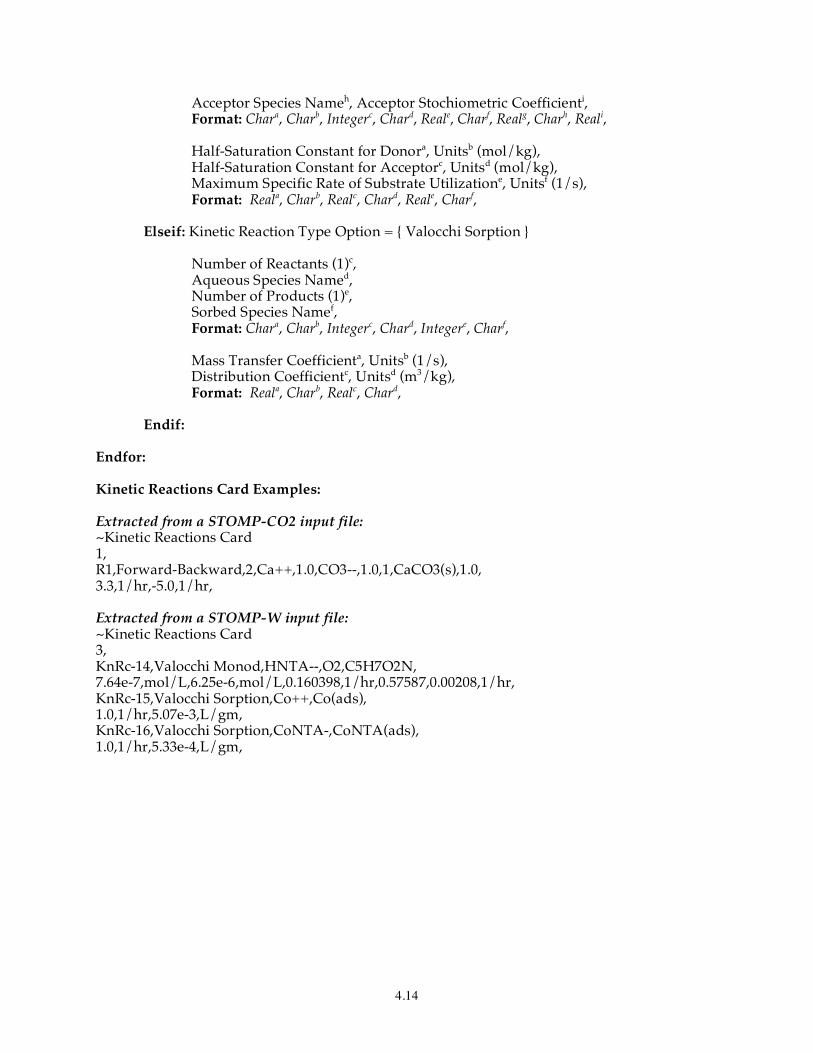
4.14

Acceptor Species Nameh, Acceptor Stochiometric Coefficienti, Format: Chara, Charb, Integerc, Chard, Reale, Charf, Realg, Charh, Reali, Half-Saturation Constant for Donora, Unitsb (mol/kg), Half-Saturation Constant for Acceptorc, Unitsd (mol/kg), Maximum Specific Rate of Substrate Utilizatione, Unitsf (1/s), Format: Reala, Charb, Realc, Chard, Reale, Charf, Elseif: Kinetic Reaction Type Option = { Valocchi Sorption }

Number of Reactants (1)c, Aqueous Species Named, Number of Products (1)e,

Sorbed Species Namef, Format: Chara, Charb, Integerc, Chard, Integere, Charf,

Mass Transfer Coefficienta, Unitsb (1/s), Distribution Coefficientc, Unitsd (m3/kg),

Format: Reala, Charb, Realc, Chard,

Endif: Endfor: Kinetic Reactions Card Examples: Extracted from a STOMP-CO2 input file: ~Kinetic Reactions Card 1, R1,Forward-Backward,2,Ca++,1.0,CO3--,1.0,1,CaCO3(s),1.0, 3.3,1/hr,-5.0,1/hr, Extracted from a STOMP-W input file: ~Kinetic Reactions Card 3, KnRc-14,Valocchi Monod,HNTA--,O2,C5H7O2N, 7.64e-7,mol/L,6.25e-6,mol/L,0.160398,1/hr,0.57587,0.00208,1/hr, KnRc-15,Valocchi Sorption,Co++,Co(ads), 1.0,1/hr,5.07e-3,L/gm, KnRc-16,Valocchi Sorption,CoNTA-,CoNTA(ads), 1.0,1/hr,5.33e-4,L/gm,

4.15

4.3.8 Lithology Card Card Titlea { ~Lithology [ Card ] } Format: Chara, For: Number of Rock/Soil Types or Scaling Groups

If: Rock/Soil or Scaling Group Name = { IJK | JKI | KIJ } Indexing

Note: A parameter value input can be replaced with an external file using the following formatting for ASCII files: file: filename or the following formattings for binary files: binary file: filename where; the external file will contain unique parameter values for each node (active or inactive) arranged according to the indexing scheme (i.e., IJK, JKI, or KIJ). Applicable units will be applied to all parameter values in the external file.

Endif: Rock/Soil or Scaling-Group Namea, Primary Mineral Specific Areab, Unitsc (m2/m3), Secondary Mineral Specific Aread, Unitse (m2/m3), Format: Chara, Realb, Charc, Reald, Chare, For: Number of Solid Species Solid Species Namea, Solid Species Volume Fraction of Rock/Soilb,

Format: Chara, Realb, Endfor: Number of Solid Species

Endfor: Number of Rock/Soil Types or Scaling Groups Lithology Card Examples: Extracted from a STOMP-CO2 input file: ~Lithology Card Glauconite Sandstone,1.e5,1/m,250.,1/m, CaCO3(s),0.0,

4.16

4.3.9 Solid Species Card

Card Titlea { ~Solid Species [ Card ] } Format: Chara, Number of Solid Speciesa, Format: Integera, For: Number of Solid Species Solid Species Namea, Species Mass Densityb, Unitsc (kg/m3) Species Molecular Weightd, Unitse (kg/m3)

Format: Chara, Realb, Charc, Reald, Chare,

Endfor: Number of Solid Species Solid Species Card Examples: Extracted from a STOMP-W input file: ~Solid Species Card 3, Co(ads),,,58.9332,kg/kmol, CoNTA(ads),,,247.0638,kg/kmol, C5H7O2N,,,113.1158,kg/kmol, Extracted from a STOMP-CO2 input file: ~Solid Species Card 1, CaCO3(s),2.709893,gm/cm^3,100.0872,kg/kmol,

4.17

4.3.10 Species Link Card

Card Titlea { ~Species Link [ Card ] } Format: Chara, Number of Species Linksa, Format: Integera, For: Number of Species Links Species Namea, Coupled Flow Component Optionb, { Aqueous pH | Aqueous Water | Gas Water | Aqueous Air | Gas Air | Aqueous CO2 | Gas CO2 | Aqueous CH4 | Gas CH4 }

Format: Chara, Charb,

Endfor: Number of Species Links Species Link Card Examples: Extracted from a STOMP-CO2 input file: ~Species Link Card 7, H+,aqueous pH, CaCO3(aq),aqueous CO2, HCO3-,aqueous CO2, CO3--,aqueous CO2, CaHCO3+,aqueous CO2, H2CO3,aqueous CO2, CO2(g),gas CO2,

5.1

5.0 Example Applications

5.1 Introduction To demonstrate the utility of the ECKEChem reactive transport module for the STOMP simulator, example applications are documented in this section using various operational modes. This section is intended to serve as a reference for reactive transport capabilities of the simulator and as a demonstration proper code execution. All selected applications in this section have been executed using other reactive transport simulators and have been published in the open literature. In serving as a reference for reactive transport capabilities this section will expand over time, as the ECKEChem module is incorporated into new operational modes and new challenging reactive transport problems are identified. The first reactive transport problem included in this section involves all three types of chemical equations: equilibrium, conservation and kinetic for a system involving aqueous flow and transport with kinetic biodegradation, cell growth, and sorption. This problem was previously reported by Parkhurst and Appelo (1999), following the original work of Tebes-Steven and Valocchi (1997; 1998).

5.2 STOMP-W: Kinetic Biodegradation, Cell Growth, and Sorption

This example problem was developed and published by Parkhurst and Appelo (1999), from an advective-dispersive-reactive transport problem, developed by Tebes-Steven and Valocchi (1997; 1998). The transport involves mobile and immobile species; where the immobile species are either bacterial cells or sorbed metals. The chemistry involves speciation, bacterially mediated degradation of an organic substrate, bacterial growth and decay, and kinetic metal sorption, including metal-ligand complexation. In brief the problem involves the steady-flow of an aqueous solution through a 10-m column, initially containing biomass. A pulse of dissolved nitrylotriacetate (Nta) and cobalt (Co) are introduced at the inlet of the column. Nta is defined to degrade in the presence of biomass and oxygen, yielding biomass growth. The equilibrium chemistry in this problem assumes activity coefficients of 1.0.

5.2.1 Problem Description

This problem involves the steady flow of an aqueous solution through a 10-m column with a pore-water velocity of 1.0 m/hr. Hydrological and mechanical properties for the system are given in Table 5.1. The aqueous solution initially within the column comprises biomass, oxygen, and carbon, at a pH of 6, but is void of Nta and Co. This problem involves 25 species, whose formula and mobility are shown in Table 5.2. The initial concentrations of species in the column, expressed in terms of aqueous molar concentrations are given in Table 5.3. The reaction network for this problem is given in Table 5.4, where equilibrium constant is defined for equilibrium type reactions and the activity of water is assumed to be 1.0.

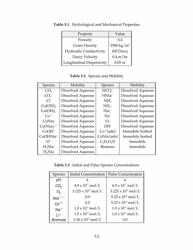
5.2

Table 5.1. Hydrological and Mechanical Properties

Property Value

Porosity 0.4 Grain Density 2500 kg/m3

Hydraulic Conductivity 100 Darcy Darcy Velocity 0.4 m/hr

Longitudinal Dispersivity 0.05 m

Table 5.2. Species and Mobility

Species Mobility Species Mobility CO2 Dissolved Aqueous HCO3

- Dissolved Aqueous CO3

-- Dissolved Aqueous HNta-- Dissolved Aqueous Cl- Dissolved Aqueous NH3 Dissolved Aqueous

Co(OH)2 Dissolved Aqueous NH4+ Dissolved Aqueous

Co(OH)3- Dissolved Aqueous Nta--- Dissolved Aqueous

Co++ Dissolved Aqueous Na+ Dissolved Aqueous CoNta- Dissolved Aqueous O2 Dissolved Aqueous

Co(Nta)2---- Dissolved Aqueous OH- Dissolved Aqueous

CoOH+ Dissolved Aqueous Co++(ads) Immobile Sorbed CoOHNta-- Dissolved Aqueous CoNta-(ads) Immobile Sorbed

H+ Dissolved Aqueous C5H7O2N Immobile H2Nta- Dissolved Aqueous Biomass Immobile H3Nta Dissolved Aqueous

Table 5.3. Initial and Pulse Species Concentrations

Species Initial Concentration Pulse Concentration

pH

6 6

CO

2 4.9 x 10-7 mol/L 4.9 x 10-7 mol/L

O

2 3.125 x 10-5 mol/L 3.125 x 10-5 mol/L

Nta 0.0 5.23 x 10-6 mol/L

Co++ 0.0 5.23 x 10-6 mol/L

Na+ 1.0 x 10-3 mol/L 1.0 x 10-3 mol/L

Cl 1.0 x 10-3 mol/L 1.0 x 10-3 mol/L

Biomass 1.36 x 10-4 mol/L 0.0

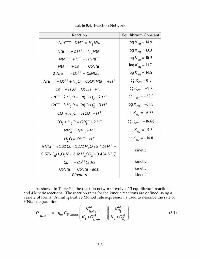
5.3

Table 5.4. Reaction Network

Reaction Equilibrium Constant

Nta + 3 H

+ = H3

Nta log K

eq= 14.9

Nta + 2 H

+ = H2

Nta log K

eq= 13.3

Nta + H+ = HNta

log Keq

= 10.3

Nta + Co++ = CoNta

log Keq

= 11.7

2 Nta + Co

++ = CoNta2

log K

eq= 14.5

Nta + Co

+++ H

2O = CoOHNta + H

+ log K

eq= 0.5

Co

+++ H

2O = CoOH + H

+ log K

eq= 9.7

Co

+++ 2 H

2O = Co(OH)

2+ 2 H

+ log K

eq= 22.9

Co

+++ 3 H

2O = Co(OH)

3+ 3 H

+ log K

eq= 31.5

CO

2+ H

2O = HCO

3+ H

+ log K

eq= 6.35

CO

2+ H

2O = CO

3+ 2 H

+ log K

eq= 16.68

NH

4+ = NH

3+ H

+ log K

eq= 9.3

H

2O = OH + H

+ log K

eq= 14.0

HNta + 1.62 O2+ 1.272 H

2O + 2.424 H

+ =

0.576 C5H

7O

2N + 3.12 H

2CO

3+ 0.424 NH

4+

kinetic

Co++ = Co

++(ads) kinetic

CoNta = CoNta (ads) kinetic

Biomass kinetic As shown in Table 5.4, the reaction network involves 13 equilibrium reactions and 4 kinetic reactions. The reaction rates for the kinetic reactions are defined using a variety of forms. A multiplicative Monod rate expression is used to describe the rate of HNta2- degradation:

RHNta

= qm

CBiomass

CHNta

M

Ks+C

HNta

M

CO2

M

Ka+C

O2

M (5.1)

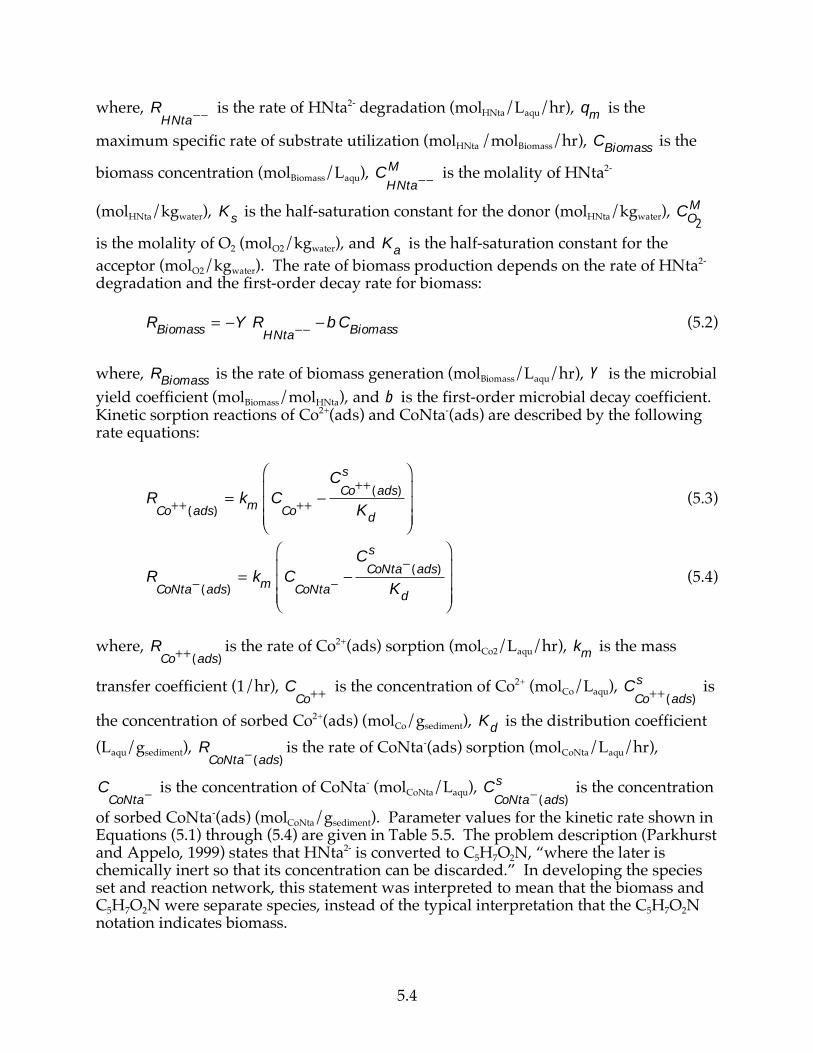
5.4

where,

RHNta

is the rate of HNta2- degradation (molHNta/Laqu/hr), q

m is the

maximum specific rate of substrate utilization (molHNta /molBiomass/hr),

C

Biomass is the

biomass concentration (molBiomass/Laqu),

CHNta

M is the molality of HNta2-

(molHNta/kgwater), Ks is the half-saturation constant for the donor (molHNta/kgwater),

C

O2

M

is the molality of O2 (molO2/kgwater), and K

a is the half-saturation constant for the

acceptor (molO2/kgwater). The rate of biomass production depends on the rate of HNta2- degradation and the first-order decay rate for biomass:

R

Biomass = Y R

HNtab C

Biomass (5.2)

where,

R

Biomass is the rate of biomass generation (molBiomass/Laqu/hr), Y is the microbial

yield coefficient (molBiomass/molHNta), and b is the first-order microbial decay coefficient. Kinetic sorption reactions of Co2+(ads) and CoNta-(ads) are described by the following rate equations:

RCo

++ (ads) = k

mC

Co++

CCo

++ (ads)

s

Kd

(5.3)

RCoNta (ads)

= km

CCoNta

CCoNta (ads)

s

Kd

(5.4)

where,

R

Co++ (ads)

is the rate of Co2+(ads) sorption (molCo2/Laqu/hr), k

m is the mass

transfer coefficient (1/hr),

CCo

++ is the concentration of Co2+ (molCo/Laqu),

C

Co++ (ads)

s is

the concentration of sorbed Co2+(ads) (molCo/gsediment), Kd is the distribution coefficient

(Laqu/gsediment), R

CoNta (ads)is the rate of CoNta-(ads) sorption (molCoNta/Laqu/hr),

CCoNta

is the concentration of CoNta- (molCoNta/Laqu), C

CoNta (ads)

s is the concentration

of sorbed CoNta-(ads) (molCoNta/gsediment). Parameter values for the kinetic rate shown in Equations (5.1) through (5.4) are given in Table 5.5. The problem description (Parkhurst and Appelo, 1999) states that HNta2- is converted to C5H7O2N, “where the later is chemically inert so that its concentration can be discarded.” In developing the species set and reaction network, this statement was interpreted to mean that the biomass and C5H7O2N were separate species, instead of the typical interpretation that the C5H7O2N notation indicates biomass.

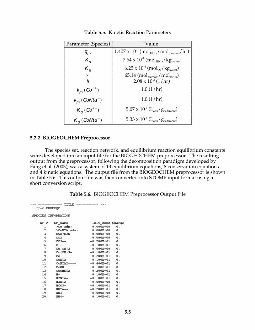
5.5

Table 5.5. Kinetic Reaction Parameters

Parameter (Species) Value

q

m 1.407 x 10-3 (molHNta/molBiomass/hr)

K

s 7.64 x 10-7 (molHNta/kgwater)

K

a 6.25 x 10-6 (molO2/kgwater)

Y 65.14 (molBiomass/molHNta)

b 2.08 x 10-3 (1/hr)

k

m(Co

++ ) 1.0 (1/hr)

k

m(CoNta ) 1.0 (1/hr)

K

d(Co

++ ) 5.07 x 10-3 (Laqu/gsediment)

K

d(CoNta ) 5.33 x 10-4 (Laqu/gsediment)

5.2.2 BIOGEOCHEM Preprocessor

The species set, reaction network, and equilibrium reaction equilibrium constants were developed into an input file for the BIOGEOCHEM preprocessor. The resulting output from the preprocessor, following the decomposition paradigm developed by Fang et al. (2003), was a system of 13 equilibrium equations, 8 conservation equations and 4 kinetic equations. The output file from the BIOGEOCHEM preprocessor is shown in Table 5.6. This output file was then converted into STOMP input format using a short conversion script.

Table 5.6. BIOGEOCHEM Preprocessor Output File

*** ------------ TITLE ----------- *** 1 from PHREEQC SPECIES INFORMATION SP # SP_name Init_conc Charge 1 >Co(ads) 0.000E+00 0. 2 >CoNTA(ads) 0.000E+00 0. 3 C5H7O2N 0.000E+00 0. 4 CO2 0.000E+00 0. 5 CO3-- -0.200E+01 0. 6 Cl- -0.100E+01 0. 7 Co(OH)2 0.000E+00 0. 8 Co(OH)3- -0.100E+01 0. 9 Co++ 0.200E+01 0. 10 CoNTA- -0.100E+01 0. 11 CoNTA2---- -0.400E+01 0. 12 CoOH+ 0.100E+01 0. 13 CoOHNTA-- -0.200E+01 0. 14 H+ 0.100E+01 0. 15 H2NTA- -0.100E+01 0. 16 H3NTA 0.000E+00 0. 17 HCO3- -0.100E+01 0. 18 HNTA-- -0.200E+01 0. 19 NH3 0.000E+00 0. 20 NH4+ 0.100E+01 0.

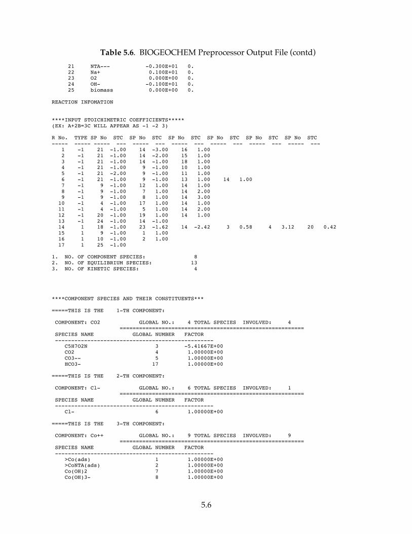
5.6

Table 5.6. BIOGEOCHEM Preprocessor Output File (contd) 21 NTA--- -0.300E+01 0. 22 Na+ 0.100E+01 0. 23 O2 0.000E+00 0. 24 OH- -0.100E+01 0. 25 biomass 0.000E+00 0. REACTION INFOMATION ****INPUT STOICHIMETRIC COEFFICIENTS***** (EX: A+2B=3C WILL APPEAR AS -1 -2 3) R No. TYPE SP No STC SP No STC SP No STC SP No STC SP No STC SP No STC ----- ----- ----- --- ----- --- ----- --- ----- --- ----- --- ----- --- 1 -1 21 -1.00 14 -3.00 16 1.00 2 -1 21 -1.00 14 -2.00 15 1.00 3 -1 21 -1.00 14 -1.00 18 1.00 4 -1 21 -1.00 9 -1.00 10 1.00 5 -1 21 -2.00 9 -1.00 11 1.00 6 -1 21 -1.00 9 -1.00 13 1.00 14 1.00 7 -1 9 -1.00 12 1.00 14 1.00 8 -1 9 -1.00 7 1.00 14 2.00 9 -1 9 -1.00 8 1.00 14 3.00 10 -1 4 -1.00 17 1.00 14 1.00 11 -1 4 -1.00 5 1.00 14 2.00 12 -1 20 -1.00 19 1.00 14 1.00 13 -1 24 -1.00 14 -1.00 14 1 18 -1.00 23 -1.62 14 -2.42 3 0.58 4 3.12 20 0.42 15 1 9 -1.00 1 1.00 16 1 10 -1.00 2 1.00 17 1 25 -1.00 1. NO. OF COMPONENT SPECIES: 8 2. NO. OF EQUILIBRIUM SPECIES: 13 3. NO. OF KINETIC SPECIES: 4 ****COMPONENT SPECIES AND THEIR CONSTITUENTS*** =====THIS IS THE 1-TH COMPONENT: COMPONENT: CO2 GLOBAL NO.: 4 TOTAL SPECIES INVOLVED: 4 ========================================================= SPECIES NAME GLOBAL NUMBER FACTOR ------------------------------------------------- C5H7O2N 3 -5.41667E+00 CO2 4 1.00000E+00 CO3-- 5 1.00000E+00 HCO3- 17 1.00000E+00 =====THIS IS THE 2-TH COMPONENT: COMPONENT: Cl- GLOBAL NO.: 6 TOTAL SPECIES INVOLVED: 1 ========================================================= SPECIES NAME GLOBAL NUMBER FACTOR ------------------------------------------------- Cl- 6 1.00000E+00 =====THIS IS THE 3-TH COMPONENT: COMPONENT: Co++ GLOBAL NO.: 9 TOTAL SPECIES INVOLVED: 9 ========================================================= SPECIES NAME GLOBAL NUMBER FACTOR ------------------------------------------------- >Co(ads) 1 1.00000E+00 >CoNTA(ads) 2 1.00000E+00 Co(OH)2 7 1.00000E+00 Co(OH)3- 8 1.00000E+00

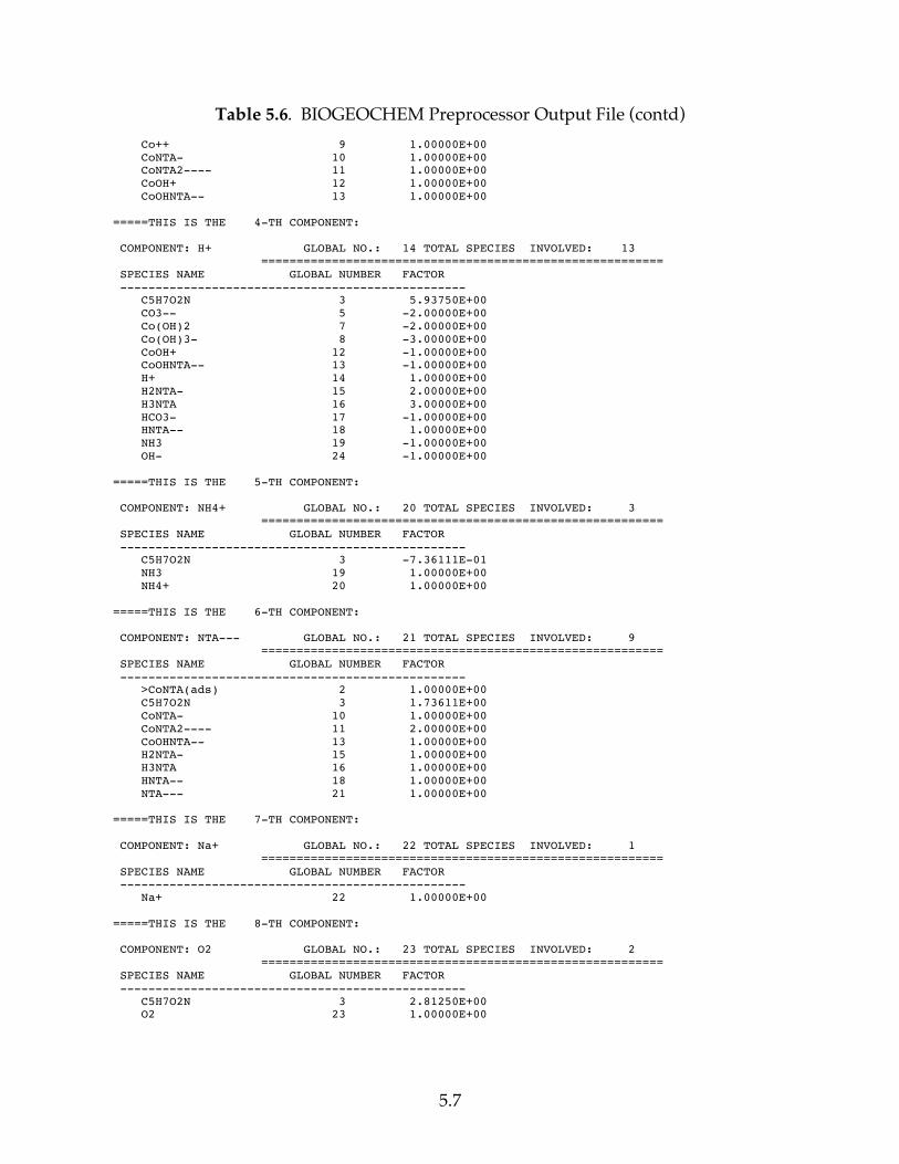
5.7

Table 5.6. BIOGEOCHEM Preprocessor Output File (contd) Co++ 9 1.00000E+00 CoNTA- 10 1.00000E+00 CoNTA2---- 11 1.00000E+00 CoOH+ 12 1.00000E+00 CoOHNTA-- 13 1.00000E+00 =====THIS IS THE 4-TH COMPONENT: COMPONENT: H+ GLOBAL NO.: 14 TOTAL SPECIES INVOLVED: 13 ========================================================= SPECIES NAME GLOBAL NUMBER FACTOR ------------------------------------------------- C5H7O2N 3 5.93750E+00 CO3-- 5 -2.00000E+00 Co(OH)2 7 -2.00000E+00 Co(OH)3- 8 -3.00000E+00 CoOH+ 12 -1.00000E+00 CoOHNTA-- 13 -1.00000E+00 H+ 14 1.00000E+00 H2NTA- 15 2.00000E+00 H3NTA 16 3.00000E+00 HCO3- 17 -1.00000E+00 HNTA-- 18 1.00000E+00 NH3 19 -1.00000E+00 OH- 24 -1.00000E+00 =====THIS IS THE 5-TH COMPONENT: COMPONENT: NH4+ GLOBAL NO.: 20 TOTAL SPECIES INVOLVED: 3 ========================================================= SPECIES NAME GLOBAL NUMBER FACTOR ------------------------------------------------- C5H7O2N 3 -7.36111E-01 NH3 19 1.00000E+00 NH4+ 20 1.00000E+00 =====THIS IS THE 6-TH COMPONENT: COMPONENT: NTA--- GLOBAL NO.: 21 TOTAL SPECIES INVOLVED: 9 ========================================================= SPECIES NAME GLOBAL NUMBER FACTOR ------------------------------------------------- >CoNTA(ads) 2 1.00000E+00 C5H7O2N 3 1.73611E+00 CoNTA- 10 1.00000E+00 CoNTA2---- 11 2.00000E+00 CoOHNTA-- 13 1.00000E+00 H2NTA- 15 1.00000E+00 H3NTA 16 1.00000E+00 HNTA-- 18 1.00000E+00 NTA--- 21 1.00000E+00 =====THIS IS THE 7-TH COMPONENT: COMPONENT: Na+ GLOBAL NO.: 22 TOTAL SPECIES INVOLVED: 1 ========================================================= SPECIES NAME GLOBAL NUMBER FACTOR ------------------------------------------------- Na+ 22 1.00000E+00 =====THIS IS THE 8-TH COMPONENT: COMPONENT: O2 GLOBAL NO.: 23 TOTAL SPECIES INVOLVED: 2 ========================================================= SPECIES NAME GLOBAL NUMBER FACTOR ------------------------------------------------- C5H7O2N 3 2.81250E+00 O2 23 1.00000E+00

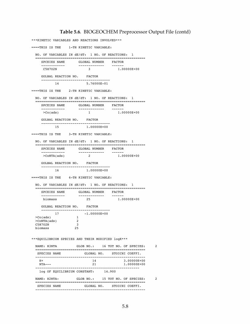
5.8

Table 5.6. BIOGEOCHEM Preprocessor Output File (contd) ***KINETIC VARIABLES AND REACTIONS INVOLVED*** ====THIS IS THE 1-TH KINETIC VARIABLE: NO. OF VARIABLES IN dE/dT: 1 NO. OF REACTIONS: 1 ======================================================== SPCEIES NAME GLOBAL NUMBER FACTOR ------------ ------------- ------ C5H7O2N 3 1.00000E+00 GOLBAL REACTION NO. FACTOR ----------------------------------- 14 5.76000E-01 ====THIS IS THE 2-TH KINETIC VARIABLE: NO. OF VARIABLES IN dE/dT: 1 NO. OF REACTIONS: 1 ======================================================== SPCEIES NAME GLOBAL NUMBER FACTOR ------------ ------------- ------ >Co(ads) 1 1.00000E+00 GOLBAL REACTION NO. FACTOR ----------------------------------- 15 1.00000E+00 ====THIS IS THE 3-TH KINETIC VARIABLE: NO. OF VARIABLES IN dE/dT: 1 NO. OF REACTIONS: 1 ======================================================== SPCEIES NAME GLOBAL NUMBER FACTOR ------------ ------------- ------ >CoNTA(ads) 2 1.00000E+00 GOLBAL REACTION NO. FACTOR ----------------------------------- 16 1.00000E+00 ====THIS IS THE 4-TH KINETIC VARIABLE: NO. OF VARIABLES IN dE/dT: 1 NO. OF REACTIONS: 1 ======================================================== SPCEIES NAME GLOBAL NUMBER FACTOR ------------ ------------- ------ biomass 25 1.00000E+00 GOLBAL REACTION NO. FACTOR ----------------------------------- 17 -1.00000E+00 >Co(ads) 1 >CoNTA(ads) 2 C5H7O2N 3 biomass 25 ***EQUILIBRIUM SPECIES AND THEIR MODIFIED logK*** NAME: H3NTA GLOB NO.: 16 TOT NO. OF SPECIES: 2 ======================================================== SPECIES NAME GLOBAL NO. STOICHI COEFFI. -------------------------------------------------------- H+ 14 3.00000E+00 NTA--- 21 1.00000E+00 ----------------------------------------------------- log OF EQUILIBRIUM CONSTANT: 14.900 NAME: H2NTA- GLOB NO.: 15 TOT NO. OF SPECIES: 2 ======================================================== SPECIES NAME GLOBAL NO. STOICHI COEFFI. --------------------------------------------------------

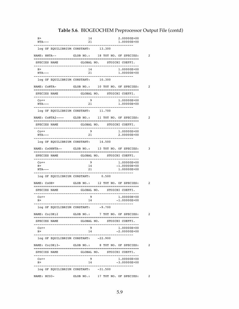
5.9

Table 5.6. BIOGEOCHEM Preprocessor Output File (contd) H+ 14 2.00000E+00 NTA--- 21 1.00000E+00 ----------------------------------------------------- log OF EQUILIBRIUM CONSTANT: 13.300 NAME: HNTA-- GLOB NO.: 18 TOT NO. OF SPECIES: 2 ======================================================== SPECIES NAME GLOBAL NO. STOICHI COEFFI. -------------------------------------------------------- H+ 14 1.00000E+00 NTA--- 21 1.00000E+00 ----------------------------------------------------- log OF EQUILIBRIUM CONSTANT: 10.300 NAME: CoNTA- GLOB NO.: 10 TOT NO. OF SPECIES: 2 ======================================================== SPECIES NAME GLOBAL NO. STOICHI COEFFI. -------------------------------------------------------- Co++ 9 1.00000E+00 NTA--- 21 1.00000E+00 ----------------------------------------------------- log OF EQUILIBRIUM CONSTANT: 11.700 NAME: CoNTA2---- GLOB NO.: 11 TOT NO. OF SPECIES: 2 ======================================================== SPECIES NAME GLOBAL NO. STOICHI COEFFI. -------------------------------------------------------- Co++ 9 1.00000E+00 NTA--- 21 2.00000E+00 ----------------------------------------------------- log OF EQUILIBRIUM CONSTANT: 14.500 NAME: CoOHNTA-- GLOB NO.: 13 TOT NO. OF SPECIES: 3 ======================================================== SPECIES NAME GLOBAL NO. STOICHI COEFFI. -------------------------------------------------------- Co++ 9 1.00000E+00 H+ 14 -1.00000E+00 NTA--- 21 1.00000E+00 ----------------------------------------------------- log OF EQUILIBRIUM CONSTANT: 0.500 NAME: CoOH+ GLOB NO.: 12 TOT NO. OF SPECIES: 2 ======================================================== SPECIES NAME GLOBAL NO. STOICHI COEFFI. -------------------------------------------------------- Co++ 9 1.00000E+00 H+ 14 -1.00000E+00 ----------------------------------------------------- log OF EQUILIBRIUM CONSTANT: -9.700 NAME: Co(OH)2 GLOB NO.: 7 TOT NO. OF SPECIES: 2 ======================================================== SPECIES NAME GLOBAL NO. STOICHI COEFFI. -------------------------------------------------------- Co++ 9 1.00000E+00 H+ 14 -2.00000E+00 ----------------------------------------------------- log OF EQUILIBRIUM CONSTANT: -22.900 NAME: Co(OH)3- GLOB NO.: 8 TOT NO. OF SPECIES: 2 ======================================================== SPECIES NAME GLOBAL NO. STOICHI COEFFI. -------------------------------------------------------- Co++ 9 1.00000E+00 H+ 14 -3.00000E+00 ----------------------------------------------------- log OF EQUILIBRIUM CONSTANT: -31.500 NAME: HCO3- GLOB NO.: 17 TOT NO. OF SPECIES: 2

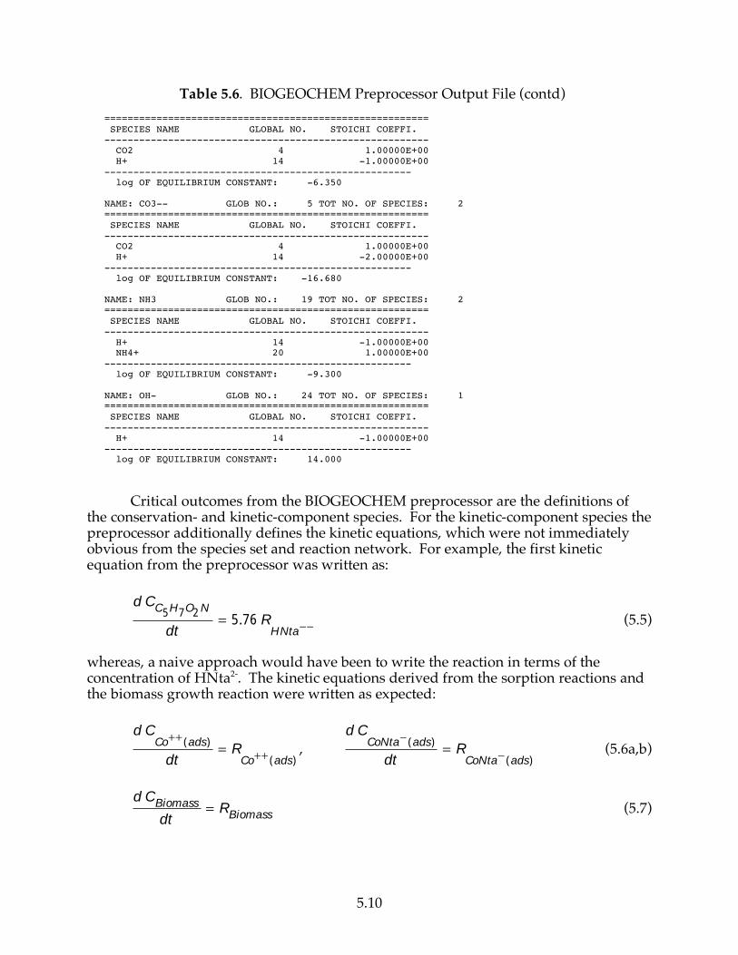
5.10

Table 5.6. BIOGEOCHEM Preprocessor Output File (contd) ======================================================== SPECIES NAME GLOBAL NO. STOICHI COEFFI. -------------------------------------------------------- CO2 4 1.00000E+00 H+ 14 -1.00000E+00 ----------------------------------------------------- log OF EQUILIBRIUM CONSTANT: -6.350 NAME: CO3-- GLOB NO.: 5 TOT NO. OF SPECIES: 2 ======================================================== SPECIES NAME GLOBAL NO. STOICHI COEFFI. -------------------------------------------------------- CO2 4 1.00000E+00 H+ 14 -2.00000E+00 ----------------------------------------------------- log OF EQUILIBRIUM CONSTANT: -16.680 NAME: NH3 GLOB NO.: 19 TOT NO. OF SPECIES: 2 ======================================================== SPECIES NAME GLOBAL NO. STOICHI COEFFI. -------------------------------------------------------- H+ 14 -1.00000E+00 NH4+ 20 1.00000E+00 ----------------------------------------------------- log OF EQUILIBRIUM CONSTANT: -9.300 NAME: OH- GLOB NO.: 24 TOT NO. OF SPECIES: 1 ======================================================== SPECIES NAME GLOBAL NO. STOICHI COEFFI. -------------------------------------------------------- H+ 14 -1.00000E+00 ----------------------------------------------------- log OF EQUILIBRIUM CONSTANT: 14.000 Critical outcomes from the BIOGEOCHEM preprocessor are the definitions of the conservation- and kinetic-component species. For the kinetic-component species the preprocessor additionally defines the kinetic equations, which were not immediately obvious from the species set and reaction network. For example, the first kinetic equation from the preprocessor was written as:

d CC5H7O2N

dt = 5.76 R

HNta (5.5)

whereas, a naive approach would have been to write the reaction in terms of the concentration of HNta2-. The kinetic equations derived from the sorption reactions and the biomass growth reaction were written as expected:

d CCo

++ (ads)

dt = R

Co++ (ads)

,

d CCoNta (ads)

dt = R

CoNta (ads) (5.6a,b)

d CBiomass

dt = R

Biomass (5.7)

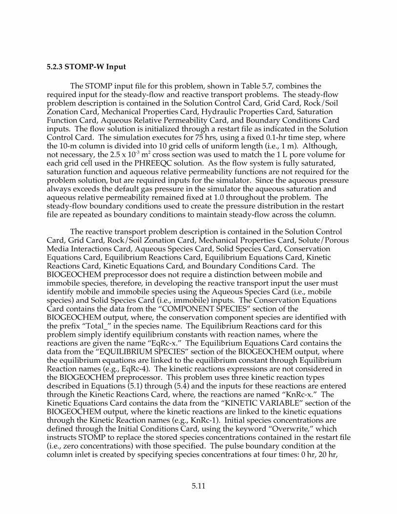
5.11

5.2.3 STOMP-W Input The STOMP input file for this problem, shown in Table 5.7, combines the required input for the steady-flow and reactive transport problems. The steady-flow problem description is contained in the Solution Control Card, Grid Card, Rock/Soil Zonation Card, Mechanical Properties Card, Hydraulic Properties Card, Saturation Function Card, Aqueous Relative Permeability Card, and Boundary Conditions Card inputs. The flow solution is initialized through a restart file as indicated in the Solution Control Card. The simulation executes for 75 hrs, using a fixed 0.1-hr time step, where the 10-m column is divided into 10 grid cells of uniform length (i.e., 1 m). Although, not necessary, the 2.5 x 10-3 m2 cross section was used to match the 1 L pore volume for each grid cell used in the PHREEQC solution. As the flow system is fully saturated, saturation function and aqueous relative permeability functions are not required for the problem solution, but are required inputs for the simulator. Since the aqueous pressure always exceeds the default gas pressure in the simulator the aqueous saturation and aqueous relative permeability remained fixed at 1.0 throughout the problem. The steady-flow boundary conditions used to create the pressure distribution in the restart file are repeated as boundary conditions to maintain steady-flow across the column. The reactive transport problem description is contained in the Solution Control Card, Grid Card, Rock/Soil Zonation Card, Mechanical Properties Card, Solute/Porous Media Interactions Card, Aqueous Species Card, Solid Species Card, Conservation Equations Card, Equilibrium Reactions Card, Equilibrium Equations Card, Kinetic Reactions Card, Kinetic Equations Card, and Boundary Conditions Card. The BIOGEOCHEM preprocessor does not require a distinction between mobile and immobile species, therefore, in developing the reactive transport input the user must identify mobile and immobile species using the Aqueous Species Card (i.e., mobile species) and Solid Species Card (i.e., immobile) inputs. The Conservation Equations Card contains the data from the “COMPONENT SPECIES” section of the BIOGEOCHEM output, where, the conservation component species are identified with the prefix “Total_” in the species name. The Equilibrium Reactions card for this problem simply identify equilibrium constants with reaction names, where the reactions are given the name “EqRc-x.” The Equilibrium Equations Card contains the data from the “EQUILIBRIUM SPECIES” section of the BIOGEOCHEM output, where the equilibrium equations are linked to the equilibrium constant through Equilibrium Reaction names (e.g., EqRc-4). The kinetic reactions expressions are not considered in the BIOGEOCHEM preprocessor. This problem uses three kinetic reaction types described in Equations (5.1) through (5.4) and the inputs for these reactions are entered through the Kinetic Reactions Card, where, the reactions are named “KnRc-x.” The Kinetic Equations Card contains the data from the “KINETIC VARIABLE” section of the BIOGEOCHEM output, where the kinetic reactions are linked to the kinetic equations through the Kinetic Reaction names (e.g., KnRc-1). Initial species concentrations are defined through the Initial Conditions Card, using the keyword “Overwrite,” which instructs STOMP to replace the stored species concentrations contained in the restart file (i.e., zero concentrations) with those specified. The pulse boundary condition at the column inlet is created by specifying species concentrations at four times: 0 hr, 20 hr,

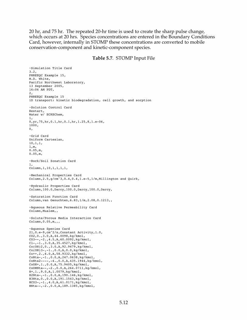
5.12

20 hr, and 75 hr. The repeated 20-hr time is used to create the sharp pulse change, which occurs at 20 hrs. Species concentrations are entered in the Boundary Conditions Card, however, internally in STOMP these concentrations are converted to mobile conservation-component and kinetic-component species.

Table 5.7. STOMP Input File ~Simulation Title Card 3.2, PHREEQC Example 15, M.D. White, Pacific Northwest Laboratory, 13 September 2005, 16:06 AM PDT, 2, PHREEQC Example 15 1D transport: kinetic biodegradation, cell growth, and sorption ~Solution Control Card Restart, Water w/ ECKEChem, 1, 0,yr,75,hr,0.1,hr,0.1,hr,1.25,8,1.e-06, 1000, 0, ~Grid Card Uniform Cartesian, 10,1,1, 1,m, 0.05,m, 0.05,m, ~Rock/Soil Zonation Card 1, Column,1,10,1,1,1,1, ~Mechanical Properties Card Column,2.5,g/cm^3,0.4,0.4,1.e-5,1/m,Millington and Quirk, ~Hydraulic Properties Card Column,100.0,Darcy,100.0,Darcy,100.0,Darcy, ~Saturation Function Card Column,van Genuchten,6.83,1/m,2.08,0.1213,, ~Aqueous Relative Permeability Card Column,Mualem,, ~Solute/Porous Media Interaction Card Column,0.05,m,,, ~Aqueous Species Card 21,0.e-9,cm^2/s,Constant Activity,1.0, CO2,0.,3.0,A,44.0098,kg/kmol, CO3--,-2.,4.5,A,60.0092,kg/kmol, Cl-,-1.,3.0,A,35.4527,kg/kmol, Co(OH)2,0.,3.0,A,92.9479,kg/kmol, Co(OH)3-,-1.,0.0,A,0.0,kg/kmol, Co++,2.,6.0,A,58.9332,kg/kmol, CoNta-,-1.,0.0,A,247.0638,kg/kmol, CoNta2----,-4.,0.0,A,435.1944,kg/kmol, CoOH+,1.,0.0,A,75.9405,kg/kmol, CoOHNta--,-2.,0.0,A,264.0711,kg/kmol, H+,1.,9.0,A,1.0079,kg/kmol, H2Nta-,-1.,0.0,A,190.146,kg/kmol, H3Nta,0.,0.0,A,191.1543,kg/kmol, HCO3-,-1.,4.0,A,61.0171,kg/kmol, HNta--,-2.,0.0,A,189.1385,kg/kmol,

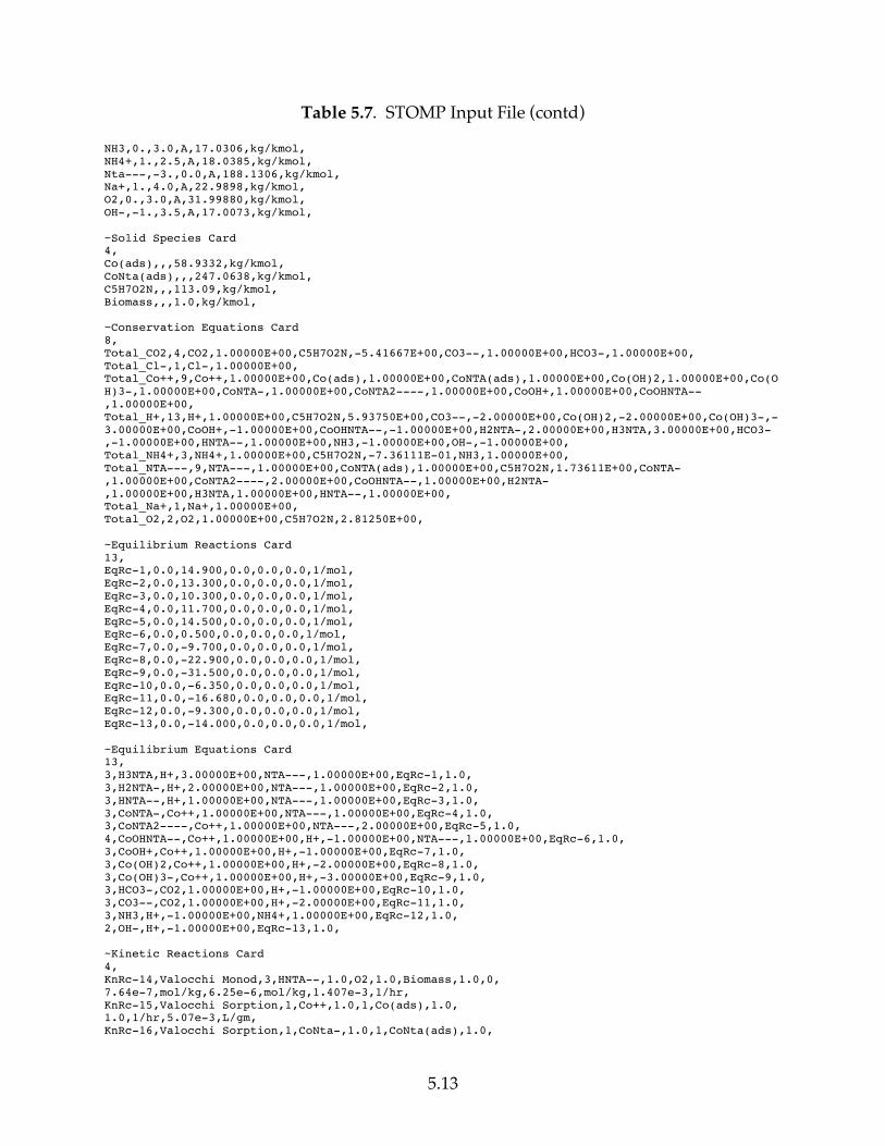
5.13

Table 5.7. STOMP Input File (contd) NH3,0.,3.0,A,17.0306,kg/kmol, NH4+,1.,2.5,A,18.0385,kg/kmol, Nta---,-3.,0.0,A,188.1306,kg/kmol, Na+,1.,4.0,A,22.9898,kg/kmol, O2,0.,3.0,A,31.99880,kg/kmol, OH-,-1.,3.5,A,17.0073,kg/kmol, ~Solid Species Card 4, Co(ads),,,58.9332,kg/kmol, CoNta(ads),,,247.0638,kg/kmol, C5H7O2N,,,113.09,kg/kmol, Biomass,,,1.0,kg/kmol, ~Conservation Equations Card 8, Total_CO2,4,CO2,1.00000E+00,C5H7O2N,-5.41667E+00,CO3--,1.00000E+00,HCO3-,1.00000E+00, Total_Cl-,1,Cl-,1.00000E+00, Total_Co++,9,Co++,1.00000E+00,Co(ads),1.00000E+00,CoNTA(ads),1.00000E+00,Co(OH)2,1.00000E+00,Co(OH)3-,1.00000E+00,CoNTA-,1.00000E+00,CoNTA2----,1.00000E+00,CoOH+,1.00000E+00,CoOHNTA--,1.00000E+00, Total_H+,13,H+,1.00000E+00,C5H7O2N,5.93750E+00,CO3--,-2.00000E+00,Co(OH)2,-2.00000E+00,Co(OH)3-,-3.00000E+00,CoOH+,-1.00000E+00,CoOHNTA--,-1.00000E+00,H2NTA-,2.00000E+00,H3NTA,3.00000E+00,HCO3-,-1.00000E+00,HNTA--,1.00000E+00,NH3,-1.00000E+00,OH-,-1.00000E+00, Total_NH4+,3,NH4+,1.00000E+00,C5H7O2N,-7.36111E-01,NH3,1.00000E+00, Total_NTA---,9,NTA---,1.00000E+00,CoNTA(ads),1.00000E+00,C5H7O2N,1.73611E+00,CoNTA-,1.00000E+00,CoNTA2----,2.00000E+00,CoOHNTA--,1.00000E+00,H2NTA-,1.00000E+00,H3NTA,1.00000E+00,HNTA--,1.00000E+00, Total_Na+,1,Na+,1.00000E+00, Total_O2,2,O2,1.00000E+00,C5H7O2N,2.81250E+00, ~Equilibrium Reactions Card 13, EqRc-1,0.0,14.900,0.0,0.0,0.0,1/mol, EqRc-2,0.0,13.300,0.0,0.0,0.0,1/mol, EqRc-3,0.0,10.300,0.0,0.0,0.0,1/mol, EqRc-4,0.0,11.700,0.0,0.0,0.0,1/mol, EqRc-5,0.0,14.500,0.0,0.0,0.0,1/mol, EqRc-6,0.0,0.500,0.0,0.0,0.0,1/mol, EqRc-7,0.0,-9.700,0.0,0.0,0.0,1/mol, EqRc-8,0.0,-22.900,0.0,0.0,0.0,1/mol, EqRc-9,0.0,-31.500,0.0,0.0,0.0,1/mol, EqRc-10,0.0,-6.350,0.0,0.0,0.0,1/mol, EqRc-11,0.0,-16.680,0.0,0.0,0.0,1/mol, EqRc-12,0.0,-9.300,0.0,0.0,0.0,1/mol, EqRc-13,0.0,-14.000,0.0,0.0,0.0,1/mol, ~Equilibrium Equations Card 13, 3,H3NTA,H+,3.00000E+00,NTA---,1.00000E+00,EqRc-1,1.0, 3,H2NTA-,H+,2.00000E+00,NTA---,1.00000E+00,EqRc-2,1.0, 3,HNTA--,H+,1.00000E+00,NTA---,1.00000E+00,EqRc-3,1.0, 3,CoNTA-,Co++,1.00000E+00,NTA---,1.00000E+00,EqRc-4,1.0, 3,CoNTA2----,Co++,1.00000E+00,NTA---,2.00000E+00,EqRc-5,1.0, 4,CoOHNTA--,Co++,1.00000E+00,H+,-1.00000E+00,NTA---,1.00000E+00,EqRc-6,1.0, 3,CoOH+,Co++,1.00000E+00,H+,-1.00000E+00,EqRc-7,1.0, 3,Co(OH)2,Co++,1.00000E+00,H+,-2.00000E+00,EqRc-8,1.0, 3,Co(OH)3-,Co++,1.00000E+00,H+,-3.00000E+00,EqRc-9,1.0, 3,HCO3-,CO2,1.00000E+00,H+,-1.00000E+00,EqRc-10,1.0, 3,CO3--,CO2,1.00000E+00,H+,-2.00000E+00,EqRc-11,1.0, 3,NH3,H+,-1.00000E+00,NH4+,1.00000E+00,EqRc-12,1.0, 2,OH-,H+,-1.00000E+00,EqRc-13,1.0, ~Kinetic Reactions Card 4, KnRc-14,Valocchi Monod,3,HNTA--,1.0,O2,1.0,Biomass,1.0,0, 7.64e-7,mol/kg,6.25e-6,mol/kg,1.407e-3,1/hr, KnRc-15,Valocchi Sorption,1,Co++,1.0,1,Co(ads),1.0, 1.0,1/hr,5.07e-3,L/gm, KnRc-16,Valocchi Sorption,1,CoNta-,1.0,1,CoNta(ads),1.0,

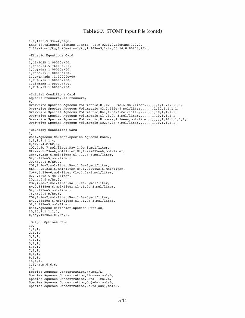
5.14

Table 5.7. STOMP Input File (contd) 1.0,1/hr,5.33e-4,L/gm, KnRc-17,Valocchi Biomass,3,HNta--,1.0,O2,1.0,Biomass,1.0,0, 7.64e-7,mol/kg,6.25e-6,mol/kg,1.407e-3,1/hr,65.14,0.00208,1/hr, ~Kinetic Equations Card 4, 1,C5H7O2N,1.00000e+00, 1,KnRc-14,5.76000e-01, 1,Co(ads),1.00000e+00, 1,KnRc-15,1.00000e+00, 1,CoNTA(ads),1.00000e+00, 1,KnRc-16,1.00000e+00, 1,Biomass,1.00000e+00, 1,KnRc-17,1.00000e+00, ~Initial Conditions Card Aqueous Pressure,Gas Pressure, 6, Overwrite Species Aqueous Volumetric,H+,0.83889e-6,mol/liter,,,,,,,1,10,1,1,1,1, Overwrite Species Aqueous Volumetric,O2,3.125e-5,mol/liter,,,,,,,1,10,1,1,1,1, Overwrite Species Aqueous Volumetric,Na+,1.0e-3,mol/liter,,,,,,,1,10,1,1,1,1, Overwrite Species Aqueous Volumetric,Cl-,1.0e-3,mol/liter,,,,,,,1,10,1,1,1,1, Overwrite Species Aqueous Volumetric,Biomass,1.36e-4,mol/liter,,,,,,,1,10,1,1,1,1, Overwrite Species Aqueous Volumetric,CO2,4.9e-7,mol/liter,,,,,,,1,10,1,1,1,1, ~Boundary Conditions Card 2, West,Aqueous Neumann,Species Aqueous Conc., 1,1,1,1,1,1,4, 0,hr,0.4,m/hr,7, CO2,4.9e-7,mol/liter,Na+,1.0e-3,mol/liter, Nta---,5.23e-6,mol/liter,H+,1.277095e-6,mol/liter, Co++,5.23e-6,mol/liter,Cl-,1.0e-3,mol/liter, O2,3.125e-5,mol/liter, 20,hr,0.4,m/hr,7, CO2,4.9e-7,mol/liter,Na+,1.0e-3,mol/liter, Nta---,5.23e-6,mol/liter,H+,1.277095e-6,mol/liter, Co++,5.23e-6,mol/liter,Cl-,1.0e-3,mol/liter, O2,3.125e-5,mol/liter, 20,hr,0.4,m/hr,5, CO2,4.9e-7,mol/liter,Na+,1.0e-3,mol/liter, H+,0.83889e-6,mol/liter,Cl-,1.0e-3,mol/liter, O2,3.125e-5,mol/liter, 75,hr,0.4,m/hr,5, CO2,4.9e-7,mol/liter,Na+,1.0e-3,mol/liter, H+,0.83889e-6,mol/liter,Cl-,1.0e-3,mol/liter, O2,3.125e-5,mol/liter, East,Aqueous Dirichlet,Species Outflow, 10,10,1,1,1,1,1, 0,day,102064.81,Pa,0, ~Output Options Card 10, 1,1,1, 2,1,1, 3,1,1, 4,1,1, 5,1,1, 6,1,1, 7,1,1, 8,1,1, 9,1,1, 10,1,1, 1,1,hr,m,6,6,6, 11, Species Aqueous Concentration,H+,mol/L, Species Aqueous Concentration,Biomass,mol/L, Species Aqueous Concentration,HNta--,mol/L, Species Aqueous Concentration,Co(ads),mol/L, Species Aqueous Concentration,CoNta(ads),mol/L,

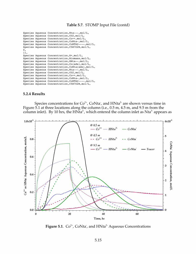
5.15

Table 5.7. STOMP Input File (contd) Species Aqueous Concentration,Nta---,mol/L, Species Aqueous Concentration,CO2,mol/L, Species Aqueous Concentration,Co++,mol/L, Species Aqueous Concentration,CoNta-,mol/L, Species Aqueous Concentration,CoNTA2----,mol/L, Species Aqueous Concentration,C5H7O2N,mol/L, 0, 11, Species Aqueous Concentration,H+,mol/L, Species Aqueous Concentration,Biomass,mol/L, Species Aqueous Concentration,HNta--,mol/L, Species Aqueous Concentration,Co(ads),mol/L, Species Aqueous Concentration,CoNta(ads),mol/L, Species Aqueous Concentration,Nta---,mol/L, Species Aqueous Concentration,CO2,mol/L, Species Aqueous Concentration,Co++,mol/L, Species Aqueous Concentration,CoNta-,mol/L, Species Aqueous Concentration,CoNTA2----,mol/L, Species Aqueous Concentration,C5H7O2N,mol/L,

5.2.4 Results Species concentrations for Co2+, CoNta-, and HNta2- are shown versus time in Figure 5.1 at three locations along the column (i.e., 0.5 m, 4.5 m, and 9.5 m from the column inlet). By 10 hrs, the HNta2-, which entered the column inlet as Nta3- appears as

Figure 5.1. Co2+, CoNta-, and HNta2- Aqueous Concentrations

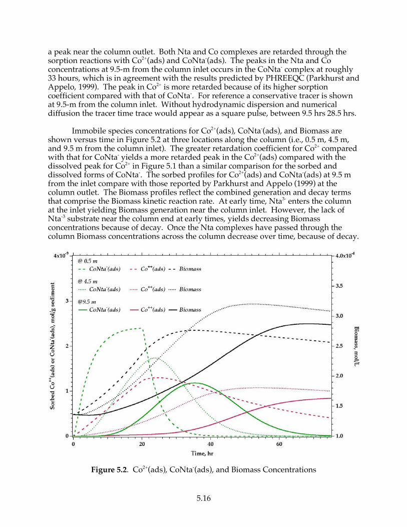
5.16

a peak near the column outlet. Both Nta and Co complexes are retarded through the sorption reactions with Co2+(ads) and CoNta-(ads). The peaks in the Nta and Co concentrations at 9.5-m from the column inlet occurs in the CoNta- complex at roughly 33 hours, which is in agreement with the results predicted by PHREEQC (Parkhurst and Appelo, 1999). The peak in Co2+ is more retarded because of its higher sorption coefficient compared with that of CoNta-. For reference a conservative tracer is shown at 9.5-m from the column inlet. Without hydrodynamic dispersion and numerical diffusion the tracer time trace would appear as a square pulse, between 9.5 hrs 28.5 hrs. Immobile species concentrations for Co2+(ads), CoNta-(ads), and Biomass are shown versus time in Figure 5.2 at three locations along the column (i.e., 0.5 m, 4.5 m, and 9.5 m from the column inlet). The greater retardation coefficient for Co2+ compared with that for CoNta- yields a more retarded peak in the Co2+(ads) compared with the dissolved peak for Co2+ in Figure 5.1 than a similar comparison for the sorbed and dissolved forms of CoNta-. The sorbed profiles for Co2+(ads) and CoNta-(ads) at 9.5 m from the inlet compare with those reported by Parkhurst and Appelo (1999) at the column outlet. The Biomass profiles reflect the combined generation and decay terms that comprise the Biomass kinetic reaction rate. At early time, Nta3- enters the column at the inlet yielding Biomass generation near the column inlet. However, the lack of Nta-3 substrate near the column end at early times, yields decreasing Biomass concentrations because of decay. Once the Nta complexes have passed through the column Biomass concentrations across the column decrease over time, because of decay.

Figure 5.2. Co2+(ads), CoNta-(ads), and Biomass Concentrations

6. References Fang, Y., G.-T. Yeh, and W. D. Burgos. 2003. "A general paradigm to model reaction-based biogeochemical processes in batch systems." Water Resources Research, 39(4):1083-1107. Parkhurst, D. L. and C. A. J. Appelo. 1999. User’s Guide to PHREEQC (Version 2) – A Computer Program for Speciation, Batch Reaction, One-Dimensional Transport, and Inverse Geochemical Calculations, Water-Resources Investigation Report 99-4259, U.S. Geological Survey. Pruess, K., J. Garcia, T. Kovscek, C. Oldenburg, J. Rutqvist, C. Steefel, and T. Xu. 2002. Intercomparison of Numerical Simulation Codes for Geologic Disposal of CO2. Lawrence Berkeley National Laboratory, LBNL-51813, Berkeley, California. Saaltink, M. W., J. Carrera, annd C. Ayora. 2001. "On the behavior of approaches to simulate reactive transport." Journal of Contaminant Hydrology, 48:213-235. Steefel, C. I., and S. B. Yabusaki. 1996. OS3D/GIMRT, Software for modeling multicomponent-multidimensional reactive transport, User's manual and programmer's guide, Pacific Northwest Laboratory, PNL-11166, Richland, Washington. Tebes-Steven, C. and A. J. Valocchi. 1997. Reactive Transport Simulation with Equilibrium Speciation and Kinetic Biodegradation and Adsorption/Desorption Reactions: A Workshop on Subsurface Reactive Transport Modeling, Pacific Northwest Northwest National Laboratory, (http://terrassa.pnl.gov:2080/~kash/workshop/bmark.htm). Tebes-Steven, C. and A. J. Valocchi, J. M. van Briesen, and B. E. Rittmann. 1998. “Multicomponent transport with coupled geochemical and microbiological reactions – model description and example simulations.” Journal of Hydrology, 209:8-26. White, M. D., and M. Oostrom. 2000. STOMP Subsurface Transport Over Multiple Phases, Version 2.0, Theory Guide. Pacific Northwest National Laboratory, PNNL-12030, UC-2010, Richland, Washington. White, M. D., and M. Oostrom. 2004. STOMP Subsurface Transport Over Multiple Phases, Version 3.1, User's Guide. Pacific Northwest National Laboratory, PNNL-14478, Richland, Washington. Yeh, G. T., and V. S. Tripathi. 1989. "A critical evaluation of recent developments in hydrogeochemical transport models of reactive multichemical components." Water Resources Research, 25(1):93-108. Yeh, G. T., and V. S. Tripathi. 1991. "A model for simulating transport of reactive multispecies components: Model development and demonstration." Water Resources Research, 27:3075-3094.

Yeh, G. T., Y. Fang, and W. D. Burgos. 2005. BIOGEOCHEM 1.0: A numerical model to simulate BIOGEOCHEMical reactions under multiple phases systems in batches. Department of Civil and Environmental Engineering, technical report, University of Central Florida, Orlando, Florida. Xu, T., F. Gerard, K. Pruess, and G. Brimhall. 1997. Modeling non-isothermal multiphase multi-species reactive chemical transport in geologic media, Lawrence Berkeley National Laboratory, LBNL-40504, UC-400, Berkeley, California.