Journal of Econometrics 52 (1992) 267-287. North-Holland

Stock market volatility and the information content of stock index options

Theodore E. Day University of Texas at Dallas, Richardson, TX 750X3-0688, USA

Craig M. Lewis Vanderbilt Vniversily, Nashville, TN 37203, USA

Previous studies of the information content of the implied volatilities from the prices of call options have used a cross-sectional regression approach. This paper compares the information content of the implied volatilities from call options on the S&P 100 index to GARCH (Generalized Autoregressive Conditional Heteroscedasticity) and Exponential GARCH models of conditional volatility. By adding the implied volatility to GARCH and EGARCH models as an exogenous variable, the within-sample incremental information content of implied volatilities can be examined using a likelihood ratio test of several nested models for conditional volatility. The out-of-sample predictive content of these models is also examined by regressing expost volatility on the implied volatilities and the forecasts from GARCH and EGARCH models.

1. Introduction

The instantaneous variance of return implicit in the price of a call option can be interpreted as an ex ante forecast of the average volatility of the underlying asset over the life of the option [see Merton (1973) and Hull and White (198711. The ability of implied volatilities to predict the future volatility of an underlying asset is considered a measure of the information content of call prices. Previous research on the predictive content of implied volatilities examines the cross-sectional relation between the implied volatilities from options on individual securities and the future realized volatility of those

*This paper was presented at the ‘Statistical Models for Financial Volatility’ conference at the University of California, San Diego, the ‘Volatility and Market Structure’ conference at Vanderbilt University, the Association of Managerial Economists conference at Washington, DC, and the Wharton School, University of Pennsylvania. We would like to thank Bill Christie, Jennifer Conrad, Ron Masulis, Bill Schwert, Hans Stoll, and conference participants for many helpful comments. The authors would like to acknowledge the financial support of the UTD Management School Foundation, and the Dean’s Fund for Faculty Research and the Financial Markets Research Center at Vanderbilt University, respectively.

0304-4076/92/$05.00 0 1992-Elsevier Science Publishers B.V. All rights reserved

268 T.E. Day and C.M. Lewis, Information content of implied uolatilities

securities [see Latane and Rendleman (19761, Chiras and Manaster (1978), and Beckers (198O)l. These studies suggest that implied volatilities explain more of the cross-sectional variation in the future standard deviations of individual security returns than do historic standard deviations of returns.

This paper examines the information content of the ex ante estimates of future market volatility implicit in the prices of call options on the Standard and Poor’s 100 Index. The prediction of future market volatility is of interest due to the theoretical relation between the (conditional) expected market risk premium [see Merton (1980)] and the ex ante volatility of the market. Much of the recent research on the relation between expected risk premiums and conditional ex ante volatility has employed a statistical technique which permits asset returns to vary over time according to a generalized autoregres- sive conditional heteroscedasticity (GARCH) model [see Engle (1982) and Bollerslev (1986)]. This approach is appealing for our purposes because a time series model for the conditional volatility of an asset is estimated jointly with the risk-return relation. Recent studies which examine the time varia- tion in market risk premia using the GARCH framework find that volatility is persistent over time.’ This suggests that the GARCH model may be useful in predicting future volatility. A related model for conditional volatility is based on the empirical evidence which shows that stock returns are negatively associated with unexpected increases in volatility [see Black (19761, Christie (19821, and French, Schwert, and Stambaugh (1987)].* Nelson (1988) suggests that this negative association implies that conditional volatility has an asym- metric relation to past data. To capture this asymmetry, Nelson modifies the GARCH model by making a logarithmic transformation of the conditional variance equation, which is commonly referred to as the Exponential GARCH (EGARCH) model.

The GARCH model for volatility provides a more general framework for evaluating the incremental information content of implied volatilities than has been previously available. 3 Whereas prior research on the predictive content of implied volatilities has relied on cross-sectional regressions, the GARCH framework explicitly accounts for the time series behavior of volatility and the relation between expected returns and conditional market volatility. We examine the predictive content of implied volatility by adding it

‘French, Schwert, and Stambaugh (1987), Bollerslev, Engle, and Wooldridge (19881, Akgiray (1989), and Nelson (1988) document volatility persistence using GARCH models. It has also been noted by others using different approaches [see Officer (1973), Christie (1982), Poterba and Summers (1987), and Schwert (1989, 199OIl.

*French, Schwert, and Stambaugh (1987) also find empirical evidence consistent with a positive association between the expected risk premium on common stocks and the predictable component of market volatility using GARCH models.

3When the context is clear, we refer to the GARCH and EGARCH models as GARCH models.

T.E. Day and C.M. Lewis, Information content of implied volatilities 269

to the GARCH models as an exogenous variable. By constructing a nested model, we can statistically assess whether the implied volatility is an impor- tant determinant of conditional volatility.

Because the GARCH models are fitted over the entire sample period, these tests characterize the within-sample properties of implied volatilities. Since within-sample tests may bias the results in favor of the GARCH specifications, we also perform tests of the out-of-sample forecasting power of implied volatility and the step-ahead forecasts from GARCH models. These tests are similar to those in Fair and Shiller (19901, Pagan and Schwert (1990), and Lamoureux and Lastrapes (1990).4

The remainder of the paper is organized as follows. Section 2 discusses the time series formulation of the GARCH models and the empirical tests. The data and the procedures used to estimate these models and the estimation of the implied volatility are discussed in section 3. Section 4 presents the results for the within-sample tests of the GARCH and EGARCH models. Section 5 provides the results for the out-of-sample forecasts. The paper concludes with a brief summary in section 6.

2. Methodology

To estimate the GARCH models, we employ maximum likelihood estima- tion using the Berndt-Hall-Hall-Hausman algorithm (first derivatives are computed numerically). This class of GARCH models is particularly useful in examining the information content of implied volatilities since it permits the relation between changes in expected returns and changes in market volatility to be incorporated in the estimation procedure. Another advantage is that volatility is allowed to be a function of both exogenous and lagged dependent variables. For example, the forecast of volatility implicit in the price of a call option can be used as an exogenous variable.

The realized conditional excess return equation can be written as

R ,w-RF,=A,,+A,ht+&,,

where RM, is the return on the market portfolio (i.e., the S&P 100 index), RFt is the risk-free rate of interest, h, is the conditional standard deviation of the return on the market portfolio, and E, is a random error term that is normally distributed with mean zero and variance hf.

When high frequency data is used, it is well-known that nonsynchronous trading in the underlying index induces positive first-order serial correlation in the return series. To control for this, it is common to adjust the return

4Lamoureux and Lastrapes (1990) also examine the issue of the incremental information content of implied volatilities using call options on individual common stocks.

J.Econ K

270 TX. Day and CM Lewis, Information content of implied uolatilities

equation by including a moving average term [see French, Schwert, and Stambaugh (198711 or an autoregressive term [see Akgiray (198911. Since we use relatively low frequency data, the time series of excess returns does not have significant positive first-order serial correlation, and it is unnecessary to make an explicit adjustment. The autocorrelation function for the excess returns is reported in table 1.

To further examine this issue, we analyze two separate time series of weekly returns on the S&P 100 index. The first time series is simply the unadjusted returns computed from the closing index level, which reflects any positive serial correlation induced by nonsynchronous trading. The second time series of index returns is computed using estimates of the index level implicit in the price of stock index call options. Because call options on a stock index reflect the market’s contemporaneous estimate of the value of the underlying index, index returns computed from this second time series mitigate the impact of nonsynchronous trading. A comparison of the models using both time series permits us to evaluate the importance of nonsyn- chronous trading in weekly index returns. Since we do not find any significant differences, we report only the results for the actual return series.”

The variance equation for the GARCH formulation of the model is

hf = (Yg + a,&:_, + P,h:- ,, (2)

where (Y” > 0, (Y, > 0, and p, > 0. The conditional variance given by eq. (2) is a function of last period’s shock to the return generating process, F,_ , , and the conditional variance of returns in period t - 1, hf_,. The restrictions on the parameter values prevent negative variances. Although a more general GARCH(p, 4) model could be used, eq. (2) is consistent with the results of Akgiray (1989) who finds that, within the class of GARCH processes for market volatility, the GARCH(1, 1) specification provides the best fit using a likelihood ratio test. We are unable to reject the null hypothesis that the return-generating process follows a GARCH(l,l) process relative to its higher-order alternatives.

The conditional variance equation for the EGARCH formulation of the model is

where I/J_, equals c,_,/!r_,. Unlike the GARCH model, the parameter values are unrestricted since eq. (3) models the logarithm of variance. The conditional variance equation given by (3) is a function of the conditional variance of returns in period t - 1, hf_,, last period’s shock, E,_ ,, which has

‘The results for the implied index return series are available from the authors upon request.

T E. Day and CM Lewis, Information conlent of implied L,olatilities 271

been standardized to have unit variance, +,_ ,, and the deviation of the absolute value of $,_, from the mean absolute value, (2/7r)“‘. Including both the standardized shock and its absolute value permits the variance equation to capture any asymmetry in the relation between market returns and conditional volatility.

We analyze the information content of implied volatilities from the prices of call options on the S&P 100 index by testing the GARCH specification [given by eqs. (1) and (2)l and the EGARCH specification [given by eqs. (1) and (3)] against a more general model in which the conditional variance equations include the implied volatility (a,? ,> as an exogenous explanatory variable,

h;=a,,+a,e,2_, +p& +6& (4)

ln(hf) =LY~~+~, ln(h:_,) +cui(~rL,-i + ?(I+-rl - (2/7i)“2))

+ 61n(a,2,), (5)

where (pi is set equal to 1 in eq. (5). The implied volatility estimates used in eqs. (4) and (5) are derived from

stock index options with the shortest expiration that traded at the beginning of the week. We use these options because, among all possible options, they provide an ex ante forecast of the future volatility that is the most closely associated with a weekly time interval. The coefficient 6 in eqs. (4) and (5) can be interpreted as a measure of the incremental information which implied volatilities contribute to changes in the conditional variance of return over time. Therefore, the hypothesis that the prices of call options impound information in addition to that which can be obtained from the historic series of returns can be tested by examining the statistical significance of 6. In addition, the null hypothesis that implied volatilities do not contain informa- tion beyond that contained in past index levels can be tested using a likelihood ratio test. The unrestricted model [eqs. (41 and (511 allows implied volatility to have information content, while the restricted model [eqs. (2) and (3)l requires that future volatility depend only on past volatility and past shocks to the return-generating process.

The question of whether the GARCH and EGARCH specifications for conditional volatility contain information which is not impounded in implied volatilities can be examined by estimating eqs. (4) and (5) under the con- straint that the time series parameters [(Y, and PI in eq. (4) and 13, y, and p, in eq. (5)l are equal to zero. In this case, the conditional variance equations

272 TE. Day and C.M. Lewis, Information content of implied colatilities

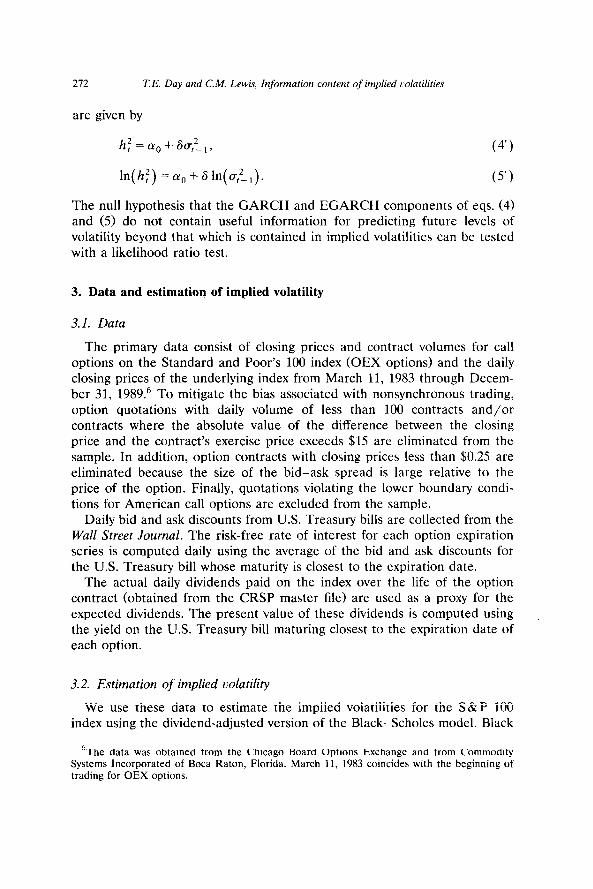
are given by

(4’)

ln(hf)=c-u,+61n(a,?,). (5’1

The null hypothesis that the GARCH and EGARCH components of eqs. (4) and (5) do not contain useful information for predicting future levels of volatility beyond that which is contained in implied volatilities can be tested with a likelihood ratio test.

3. Data and estimation of implied volatility

3.1. Data

The primary data consist of closing prices and contract volumes for call options on the Standard and Poor’s 100 index (OEX options) and the daily closing prices of the underlying index from March 11, 1983 through Decem- ber 31, 1989.6 To mitigate the bias associated with nonsynchronous trading, option quotations with daily volume of less than 100 contracts and/or contracts where the absolute value of the difference between the closing price and the contract’s exercise price exceeds $15 are eliminated from the sample. In addition, option contracts with closing prices less than $0.25 are eliminated because the size of the bid-ask spread is large relative to the price of the option. Finally, quotations violating the lower boundary condi- tions for American call options are excluded from the sample.

Daily bid and ask discounts from U.S. Treasury bills are collected from the Wall Street Journal. The risk-free rate of interest for each option expiration series is computed daily using the average of the bid and ask discounts for the U.S. Treasury bill whose maturity is closest to the expiration date.

The actual daily dividends paid on the index over the life of the option contract (obtained from the CRSP master file) are used as a proxy for the expected dividends. The present value of these dividends is computed using the yield on the U.S. Treasury bill maturing closest to the expiration date of each option.

3.2. Estimation of implied volatility

We use these data to estimate the implied volatilities for the S&P 100 index using the dividend-adjusted version of the Black-Scholes model. Black

‘The data was obtained from the Chicago Board Options Exchange and from Commodity Systems Incorporated of Boca Raton, Florida. March 11, 1983 coincides with the beginning of trading for OEX options.

T.E. Day and CM. Lewis, Information content of implied colatilities 273

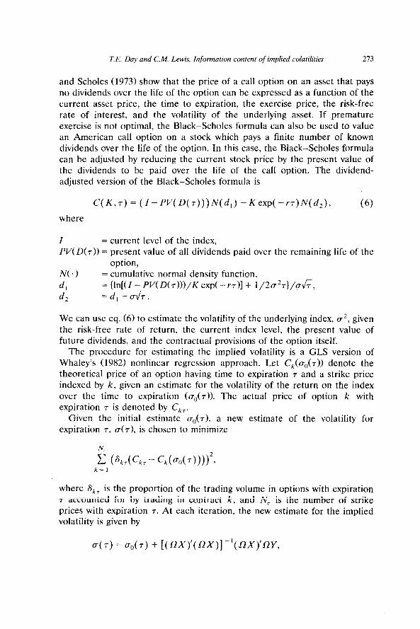
and Scholes (1973) show that the price of a call option on an asset that pays no dividends over the life of the option can be expressed as a function of the current asset price, the time to expiration, the exercise price, the risk-free rate of interest, and the volatility of the underlying asset. If premature exercise is not optimal, the Black-Scholes formula can also be used to value an American call option on a stock which pays a finite number of known dividends over the life of the option. In this case, the Black-Scholes formula can be adjusted by reducing the current stock price by the present value of the dividends to be paid over the life of the call option. The dividend- adjusted version of the Black-Scholes formula is

C(K,7) = (I-PV(D(7)))N(d,) -Kexp( -m)N(d2), (6) where

I = current level of the index, PV(D(r)) = present value of all dividends paid over the remaining life of the

NC.1

d, d,

option, = cumulative normal density function,

We can use eq. (6) to estimate the volatility of the underlying index, (T*, given the risk-free rate of return, the current index level, the present value of future dividends, and the contractual provisions of the option itself.

The procedure for estimating the implied volatility is a GLS version of Whaley’s (1982) nonlinear regression approach. Let C,(U,,(T)) denote the theoretical price of an option having time to expiration T and a strike price indexed by k, given an estimate for the volatility of the return on the index over the time to expiration (U&T)). The actual price of option k with expiration T is denoted by C,,.

Given the initial estimate u,~(T), a new estimate of the volatility for expiration T, (T(T), is chosen to minimize

where a,, is the proportion of the trading volume in options with expiration T accounted for by trading in contract k, and N, is the number of strike prices with expiration T. At each iteration, the new estimate for the implied volatility is given by

U(T) = Uo( T) + [( fix)‘( ox)] -‘( flx)‘flY,

274 T.E. Day and C.M. Lewis, Information content of implied colatilities

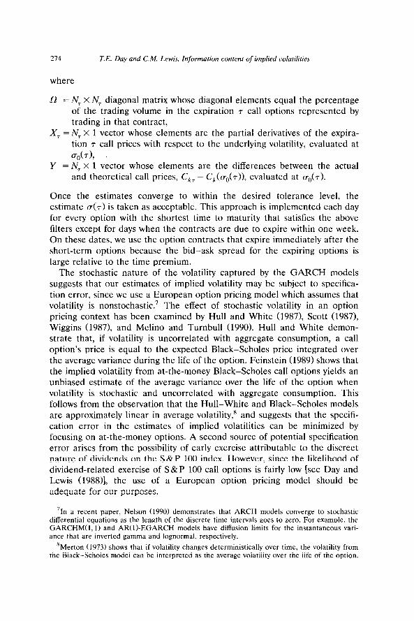
where

0 = N, X N, diagonal matrix whose diagonal elements equal the percentage of the trading volume in the expiration T call options represented by trading in that contract,

X, = N, X 1 vector whose elements are the partial derivatives of the expira- tion T call prices with respect to the underlying volatility, evaluated at

@()0(r), Y = N, X 1 vector whose elements are the differences between the actual

and theoretical call prices, C,, - C,(U,(~>>, evaluated at u”(r).

Once the estimates converge to within the desired tolerance level, the estimate (T(T) is taken as acceptable. This approach is implemented each day for every option with the shortest time to maturity that satisfies the above filters except for days when the contracts are due to expire within one week. On these dates, we use the option contracts that expire immediately after the short-term options because the bid-ask spread for the expiring options is large relative to the time premium.

The stochastic nature of the volatility captured by the GARCH models suggests that our estimates of implied volatility may be subject to specifica- tion error, since we use a European option pricing model which assumes that volatility is nonstochastic.’ The effect of stochastic volatility in an option pricing context has been examined by Hull and White (1987), Scott (1987), Wiggins (1987), and Melino and Turnbull (1990). Hull and White demon- strate that, if volatility is uncorrelated with aggregate consumption, a call option’s price is equal to the expected Black-Scholes price integrated over the average variance during the life of the option. Feinstein (1989) shows that the implied volatility from at-the-money Black-Scholes call options yields an unbiased estimate of the average variance over the life of the option when volatility is stochastic and uncorrelated with aggregate consumption. This follows from the observation that the Hull-White and Black-Scholes models are approximately linear in average volatility,8 and suggests that the specifi- cation error in the estimates of implied volatilities can be minimized by focusing on at-the-money options. A second source of potential specification error arises from the possibility of early exercise attributable to the discreet nature of dividends on the S&P 100 index. However, since the likelihood of dividend-related exercise of S&P 100 call options is fairly low [see Day and Lewis (1988)], the use of a European option pricing model should be adequate for our purposes.

‘In a recent paper, Nelson (1990) demonstrates that ARCH models converge to stochastic differential equations as the length of the discrete time intervals goes to zero. For example, the GARCHM(1, 1) and AR(l)-EGARCH models have diffusion limits for the instantaneous vari- ance that are inverted gamma and lognormal, respectively.

‘Merton (1973) shows that if volatility changes deterministically over time, the volatility from the Black-Scholes model can be interpreted as the average volatility over the life of the option.

T.E. Day and CM. Lewis, Information content of implied colatilities 275

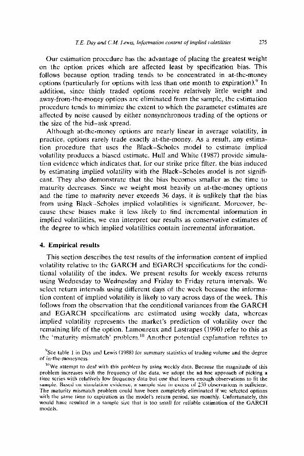
Our estimation procedure has the advantage of placing the greatest weight on the option prices which are affected least by specification bias. This follows because option trading tends to be concentrated in at-the-money options (particularly for options with less than one month to expiration).” In addition, since thinly traded options receive relatively little weight and away-from-the-money options are eliminated from the sample, the estimation procedure tends to minimize the extent to which the parameter estimates are affected by noise caused by either nonsynchronous trading of the options or the size of the bid-ask spread.

Although at-the-money options are nearly linear in average volatility, in practice, options rarely trade exactly at-the-money. As a result, any estima- tion procedure that uses the Black-Scholes model to estimate implied volatility produces a biased estimate. Hull and White (1987) provide simula- tion evidence which indicates that, for our strike price filter, the bias induced by estimating implied volatility with the Black-&holes model is not signifi- cant. They also demonstrate that the bias becomes smaller as the time to maturity decreases. Since we weight most heavily on at-the-money options and the time to maturity never exceeds 36 days, it is unlikely that the bias from using Black-Scholes implied volatilities is significant. Moreover, be- cause these biases make it less likely to find incremental information in implied volatilities, we can interpret our results as conservative estimates of the degree to which implied volatilities contain incremental information.

4. Empirical results

This section describes the test results of the information content of implied volatility relative to the GARCH and EGARCH specifications for the condi- tional volatility of the index. We present results for weekly excess returns using Wednesday to Wednesday and Friday to Friday return intervals. We select return intervals using different days of the week because the informa- tion content of implied volatility is likely to vary across days of the week. This follows from the observation that the conditional variances from the GARCH and EGARCH specifications are estimated using weekly data, whereas implied volatility represents the market’s prediction of volatility over the remaining life of the option. Lamoureux and Lastrapes (1990) refer to this as the ‘maturity mismatch’ problem. lo Another potential explanation relates to

“See table 1 in Day and Lewis (1988) for summary statistics of trading volume and the degree of in-the-moneyness.

‘“We attempt to deal with this problem by using weekly data. Because the magnitude of this problem increases with the frequency of the data, we adopt the ad hoc approach of picking a time series with relatively low frequency data but one that leaves enough observations to fit the sample. Based on simulation evidence, a sample size in excess of 250 observations is sufficient. The maturity mismatch problem could have been completely eliminated if we selected options with the same time to expiration as the model’s return period, say monthly. Unfortunately, this would have resulted in a sample size that is too small for reliable estimation of the GARCH models.

276 T.E. Day and C.M. Lewis, Information content of implied tiolatilities

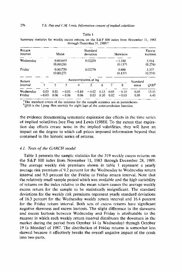
Table 1

Summary statistics for weekly excess returns on the S&P 100 index from November 11, 1983 through December 31, 1989.a

Return interval

Wednesday

Friday

Mean

0.001693 (0.00126)

0.001750 (0.00127)

Standard deviation

0.02258

0.02278

Skewness

- 1.180 (0.137)

- 0.880 (0.137)

Excess kurtosis

5.914 (0.274)

3.337 (0.274)

Return

interval 1 2

Autocorrelation at lag Standard

3 4 5 6 7 8- error Q(8)b

Wednesday 0.03 0.02 -0.01 -0.10 -0.02 0.13 0.05 -0.10 0.05 13.11 Friday - 0.03 0.06 -0.06 0.06 0.03 0.10 0.02 -0.03 0.05 6.45

aThe standard errors of the estimate for the sample statistics are in parentheses. bQ(8) is the Ljung-Box statistic for eight lags of the autocorrelation function.

the evidence documenting systematic expiration day effects in the time series of implied volatilities [see Day and Lewis (1988)]. To the extent that expira- tion day effects create noise in the implied volatilities, they will have an impact on the degree to which call prices impound information beyond that contained in the historic series of returns.

4.1. Tests of the GARCH model

Table 1 presents the sample statistics for the 319 weekly excess returns on the S&P 100 index from November 11, 1983 through December 28, 1989. The average weekly risk premiums shown in table 1 represent a yearly average risk premium of 9.2 percent for the Wednesday to Wednesday return interval and 9.5 percent for the Friday to Friday return interval. Note that the relatively small sample period which was available and the high variability of returns on the index relative to the mean return causes the average weekly excess return for the sample to be statistically insignificant. The standard deviations for the weekly risk premiums represent yearly standard deviations of 16.3 percent for the Wednesday weekly return interval and 16.4 percent for the Friday return interval. Both sets of excess returns have significant negative skewness and excess kurtosis. The slight difference in the skewness and excess kurtosis between Wednesday and Friday is attributable to the manner in which each weekly return interval distributes the downturn in the market during the period from October 14 (a Wednesday) through October 19 (a Monday) of 1987. The distribution of Friday returns is somewhat less skewed because it effectively breaks the overall negative impact of the crash into two parts.

T.E. Day and CM. Lewis, Information conlent of implied uolatilities 277

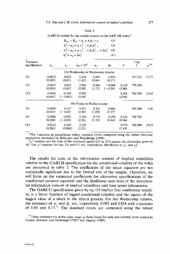
Table 2

GARCH models for the weekly returns on the S&P 100 index.”

R ,,,, -RF! = A, + A,h, + E( (1)

h:=cu,+a,e:_, +&h:m, (2)

h;=q+qe12_, f&h;_, +Sa,’ (4)

h;=q+Scr; (4’)

Variance Log specification *0 Al aoX lo4 u, PI 6 L X

2b

(2)

(4)

(4’)

(A) Wednesday to Wednesday returns

0.0072 0.071 5.428 0.093 0.854 767.321 17.77 (0.005) (0.01) (1.65) (0.84) (8.17)

0.0015 0.043 2.065 0.266 - 0.068 0.318 776.204 (0.028) (0.02) (2.98) (1.17) (GO.591 (3.00)

0.0056 -0.184 0.993 0.581 764.394 23.62 (0.001) (-0.001) (1.50) (2.94)

(B) Friday to Friday returns

(2) 0.0056 -0.167 4.951 0.101 0.806 769.286 1.00 (0.031) (- 0.02) (4.48) (1.02) (5.27)

(4) 0.0046 - 0.087 3.160 0.176 0.190 0.142 769.785 (0.028) ( - 0.02) (2.26) (1.33) (0.44) (0.96)

(4’) 0.0112 0.430 2.355 0.373 760.009 19.55 to.001) (0.001) (2.21) (1.99)

“The I-statistics in parentheses reflect standard errors computed using the robust inference procedures developed by Bollerslev and Wooldridge (1988).

“x2 statistics are for tests of the restricted model [(2) or (4’)I against the alternative given by (4). The x2 statistics for eqs. (2) and (4’) are, respectively, distributed as x: and xi.

The results for tests of the information content of implied volatilities relative to the GARCH specification for the conditional volatility of the index are presented in table 2. The coefficients of the mean equation are not statistically significant due to the limited size of the sample. Therefore, we will focus on the estimated coefficients for alternative specifications of the conditional variance equation and the likelihood ratio tests of the incremen- tal information content of implied volatilities and time series information.

The GARCH specification given by eq. (2) implies that conditional volatil- ity is a linear function of lagged conditional volatility and the square of the lagged value of a shock to the return process. For the Wednesday returns, the estimates of LY, and p, are, respectively, 0.093 and 0.854 with t-statistics of 0.84 and 8.17.” The standard errors are computed using the robust

“These estimates are in the same range as those found for daily and monthly stock returns by French, Schwert, and Stambaugh (1987) and Akgiray (1989).

J.Econ-L

278 T.E. Day and CM. Lewis, Information content of implied colatilities

inference procedures developed by Bollerslev and Wooldridge (1988). Eq. (4) includes the implied volatility from call options as an exogenous variable in the GARCH specification for the conditional volatility. For the Wednesday returns, the estimated coefficient of the implied volatility, S, is 0.318 with a t-statistic of 3.00. The significance of the estimated coefficient of implied volatility in eq. (4) suggests that the prices of call options contain incremental information regarding the conditional volatility of Wednesday returns. This conclusion is supported by a likelihood ratio test of the unrestricted model [eq. (4)] against the null hypothesis that implied volatilities contain no incremental information [eq. (211. The x2 statistic for this test has a value of 17.77, which indicates that the null hypothesis of no incremental information content may be rejected at the 0.005 level.

Although implied volatilities contain incremental information regarding the variability of the Wednesday return series, the implied volatility itself is not a sufficient statistic for the information in the GARCH model for conditional volatility. Eq. (4’) specifies the evolution of the conditional volatility as a function of the implied volatility alone. Since this model for conditional volatility is nested within eq. (4), a likelihood ratio test can be used to test the null hypothesis that the implied volatility from the prices of call options is a sufficient statistic for the conditional volatility of Wednesday excess returns. The value of the test statistic, which is distributed as x2 with two degrees of freedom, is 23.62. Therefore, the null hypothesis can be rejected at the 0.005 level.

If the implied volatility estimates are unbiased and the market for S&P 100 index options is efficient, we would expect implied volatilities to reflect all the information contained in the past series of weekly returns. The rejection of the null hypothesis that the implied volatility is a sufficient statistic for the time series of past returns may be due to the presence of measurement error which is attributable to some combination of specification error, maturity mismatch, and random estimation error. Note that although the estimated coefficient of implied volatility in eq. (4’1, 0.581, is significantly greater than zero, it is also significantly less than one. While this tends to confirm our suspicion that the implied volatilities are subject to estimation error, it is also consistent with the hypothesis that the options market overreacts to shocks to the return-generating process (e.g., during expiration weeks) causing speculative noise to be impounded in estimates of implied volatility. If this is the case, the incremental within-sample explanatory power of the GARCH terms in eq. (4) may come from the greater relative (to the squared value of the lagged shocks to the return-generating process) impor- tance of lagged conditional volatility in determining the future level of conditional volatility.

As might be expected, given the similarity of the Wednesday and Friday weekly returns, the estimated coefficients of the conditional variance specifi-

T.E. Day and CM. Lewis, Information content of implied colatilities 279

cations presented in table 2 are quite similar. For the GARCH specification [eq. (411, the estimated values of ~yi and p, are, respectively, 0.101 and 0.806 with t-statistics of 1.02 and 5.27.

In contrast to the estimate we obtain using the Wednesday return series, the estimated coefficient of implied volatility in eq. (4) is relatively small and statistically insignificant for the Friday return series. Although the estimated coefficient of implied volatility in eq. (4’) is plausible and statistically signifi- cant, indicating that implied volatilities contain information about the vari- ability of the Friday weekly return series, a likelihood ratio test of the null hypothesis that implied volatilities contain no incremental information [eq. (2)] cannot be rejected at the 0.05 level. As was the case for the Wednesday return series, the null hypothesis that implied volatility is a sufficient statistic for the information in the GARCH specification of conditional volatility can be rejected.

The failure to reject the null hypothesis that implied volatilities contain no incremental information about the volatility of the Friday return series is somewhat surprising. However, this result may well be attributable to expira- tion day effects. Day and Lewis (1988) show that on the Thursday and Friday of the week of an option expiration there is a systematic increase in the implied volatilities of call options which expire at the following expiration. They attribute this increase to price pressure created by the demand of options traders to move out of expiring option positions and into the following (month’s) expiration series. Since the Friday return series is matched with implied volatilities from closing option prices on Fridays, the existence of these expiration day biases implies that every fourth (or fifth) observation from this time series of implied volatilities may be subject to measurement error. The decrease in the magnitude of the estimated coefficient for implied volatility from Wednesday to Friday is consistent with this observation.

4.2. Estimates of the exponential GARCH model

The EGARCH model presents an alternative test of the information content of implied volatilities. Unlike the GARCH model, which constrains the conditional volatility of returns to respond symmetrically to positive and negative shocks to the return-generating process, the EGARCH model permits conditional volatility to increase (decrease) when the standardized shocks to the return-generating process I)_, are negative (positive). Conse- quently, the conditional volatility from the EGARCH model may incorporate information which is impounded in implied volatilities but which is not contained in estimates of conditional volatility from the GARCH model.

The estimates of the EGARCH model are presented in table 3. As in table 2, the results are presented for both the Wednesday and Friday return series.

280 T.E. Day and CM. Lewis, Information content of implied volatilities

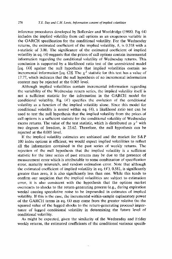
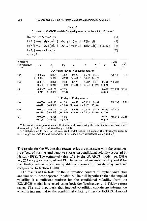
Table 3

Exponential GARCH models for weekly returns on the s&P 100 indexa

R,, -RF, = A, + A,h, + e, (1)

In(h:) =q,+P,In(h:_,) +~~,-~+Y(I~~-~I-E(I~~-~~)) (3)

In(h:) =~o+&ln(h:_,) +e$,-,+Y(I~I,-,I-E(lIL,-ll))+~~n(~~) (5) ln(hf) =a,+sln(aF) (5’)

JI, = El/h,

Variance specification

Log A0 Al ff0 PI 0 Y 6 L XZb

(3)

(5)

(5’)

(A) Wednesday to Wednesday returns

- 0.0026 0.094 - 3.62 0.529 - 0.273 0.357 776.436 8.09 (- 0.03) (0.25) (- 2.90) (3.26) (-4.13) (3.17)

0.0035 - 0.076 - 2.28 0.373 -0.282 0.210 0.351 780.480 (0.56) (-0.24) (- 1.82) (1.48) (-4.34) (1.89) (1.82)

0.0047 -0.139 -2.76 0.667 765.034 30.89 (0.71) (- 0.43) ( - 2.30) (4.01)

(3)

(5)

(5’)

(B) Friday to Friday returns

0.0056 -0.113 - 1.20 0.843 -0.121 0.194 769.192 2.58 (0.07) (-0.30) (-2.88) (15.64) (- 1.87) (2.40)

0.0057 -0.191 - 1.33 0.691 -0.170 0.114 0.142 770.481 (0.82) (-0.56) (-1.98) (3.90) (-2.11) (1.16) (1.23)

0.0090 - 0.326 - 4.02 0.49 760.142 20.68 (0.10) (- 0.74) (-5.47) (4.83)

“The r-statistics in parentheses reflect standard errors using the robust inference procedures developed by Bollerslev and Wooldridge (1988).

“x2 statistics are for tests of the restricted model [(3) or (5’)] against the alternative given by (5). The x2 statistics for eqs. (3) and (5’) are, respectively, distributed as x: and xi.

The results for the Wednesday return series are consistent with the asymmet- ric effects of positive and negative shocks on conditional volatility reported by Nelson (1988). The estimated value of 8 in the EGARCH model [eq. (3)] is -0.273 with a t-statistic of -4.13. The estimated magnitudes of y and 8 for the Friday return series are qualitatively similar to Wednesday and are comparable to Nelson (1988).

The results of the tests for the information content of implied volatilities are similar to those reported in table 2. The null hypothesis that the implied volatility is a sufficient statistic for the conditional volatility from the EGARCH model is rejected using both the Wednesday and Friday return series. The null hypothesis that implied volatilities contain no information which is incremental to the conditional volatility from the EGARCH model

TE. Day and C.M. Lewis, Information content of implied oolatilities 281

cannot be rejected for the Friday return series. However, the results from the Wednesday return series strongly reject the null hypothesis.

5. Comparison of forecasts from GARCH models and implied volatilities

In the previous section, we examined the relative power of GARCH models and implied volatilities to explain the within-sample variation in the conditional volatility of the S&P 100 index. However, since we use the entire history of implied volatilities to estimate the nested versions of the GARCH models, the results do not represent a true test of the predictive content of the two models. In this section, out-of-sample data is used to fit the GARCH models for conditional volatility. We examine whether implied volatilities contain incremental information relative to the step-ahead GARCH (and EGARCH) forecasts by regressing proxies for ex post conditional volatility on the forecasts from the alternative models.

We obtain the time series of step-ahead forecasts by estimating rolling GARCH models. The basic idea is to use a constant sample size of 410 observations to estimate a conditional volatility forecast for each date t + 1 by deleting the week t - 410 return, adding the week t return, and reestimat- ing the GARCH models. l2 After the model is reestimated, a step-ahead forecast for week t + 1 is generated. This process is repeated until we generate a sample of 319 weekly step-ahead forecasts. Note that although this time series of weekly forecasts spans the same time period examined in section 4, each forecast of weekly volatility is based entirely on the history of returns prior to the forecast period.

Forecasts of market volatility from the options market are obtained by computing the implied volatility of the S&P 100 call options having the shortest time to expiration (in excess one week) at the close of trading on the Wednesday which marks the end of the estimation sample for the GARCH models. The time series of forecasts obtained in this way is identical to the series of implied volatilities that we use in section 4 to examine the within- sample information content of implied volatility. The primary difference is that, in this section, the predictive content of the implied volatilities is compared to the forecasts using out-of-sample data.

We use each series of forecasts to predict two alternative measures of the ex post weekly volatility of the S&P 100 index. The first proxy for ex post volatility is the square of the weekly return on the index (2X). A second

‘*The estimation sample consists of the cum-dividend weekly returns on the S&P 100 index from January 1, 1976 to November 16, 1983. Since the S&P 100 index did not exist prior to the start of trading in S&P 100 index options on March 12, 1983, Standard and Poor’s retroactively created a time series of index levels beginning with January 2, 1976 using the initial population of the index.

J.Econ --M

282 T.E. Day and C.M. Lewis, Information content of implied uolatilities

proxy for ex post volatility is created by computing the daily variance for each week in the prediction sample. The daily variance is then multipied by the number of trading days in the week to generate a weekly return variance (WV). We also include the lagged value of these proxies as a form of naive forecast.

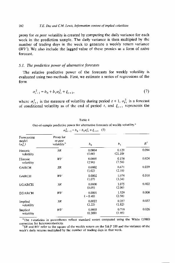
5.1. The predictive power of alternative forecasts

The relative predictive power of the forecasts for weekly volatility is evaluated using two methods. First, we estimate a series of regressions of the form

where a,‘+ 1 is the measure of volatility during period t + 1, a,$, is a forecast of conditional volatility as of the end of period t, and t,+, represents the

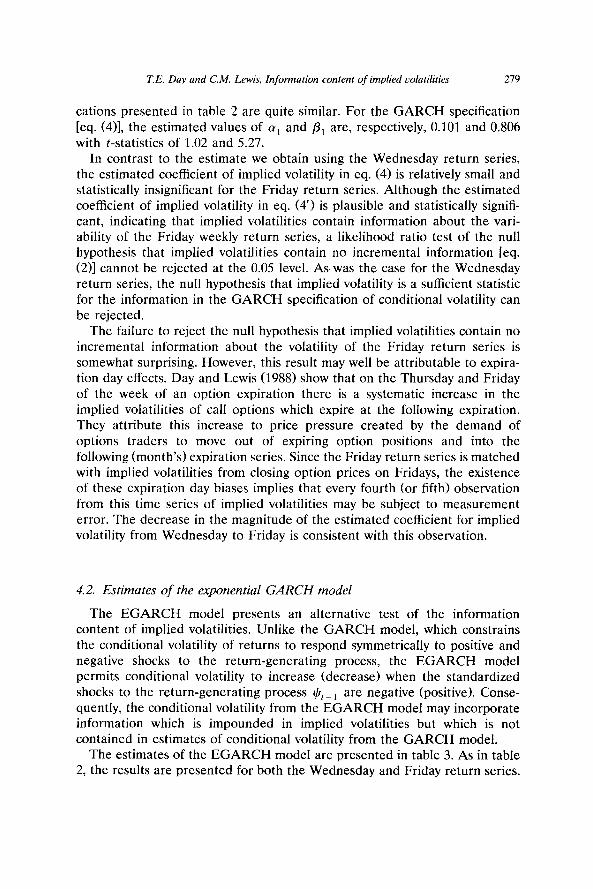
Table 4

Out-of-sample predictive power for alternative forecasts of weekly volatility.”

~;~+,=b”+~,~:,+5,+1 (7)

Forecasting model (a;*)

Historic volatility

Historic volatility

GARCH

GARCH

Proxy for ex post

volatilityb

S-R

WV

SR

WV

b,

0.0004 (5.60)

0.0005 (2.90)

0.0002 (1.02)

0.0002 (1.07)

b,

0.129 (21.18)

0.154 (7.58)

0.671 (2.10)

1.074 (3.34)

R=

0.094

0.024

0.039

0.018

EGARCH SR 0.0000 1.075 (0.05) (2.06)

0.022

EGARCH

Implied

volatility

Implied

volatility

WV - 0.0001 1.529 0.008 ( - 0.48) (2.58)

SR 0.0022 0.357 0.037 (2.22) (1.82)

WV 0.0005 0.718 0.026 (0.389) (1.95)

aThe t-statistics in parentheses reflect standard errors computed using the White (1980) correction for heteroscedasticity.

bSR and WV refer to the square of the weekly return on the S&P 100 and the variance of the week’s daily returns multiplied by the number of trading days in that week.

T.E. Day and CM Lewis, Information content of implied colatilities 283

forecast error. Pagan and Schwert (1990) note that if the forecasts of conditional volatility are unbiased, the estimate of b, will be approximately 0 and the estimate for b, will be close to 1.

Table 4 presents estimates of eq. (7) for each series of forecasts for both measures of ex post weekly volatility. Although the R’s for the reported regressions are rather low, they are similar to those reported by Pagan and Schwert for their monthly predictions of the conditional volatility of stock returns from 1900 through 1937. The forecast with the highest R2 is lagged volatility. It is interesting to note that the R2s for the GARCH model are larger than the R2s for the EGARCH model. This result may be attributable to the fact that the asymmetric relation between conditional volatility and past returns documented in section 4 is less stable over time than the GARCH effects. The estimates of b, reported in table 4 are in most cases significantly different from 0. For the GARCH regressions, the estimates of b, are both within one standard error of 1, which suggests that the GARCH forecasts of conditional volatility are unbiased. This is also true for the coefficient of the EGARCH forecast when ex post volatility is measured by the squared returns. With respect to implied volatility, the coefficient b, is within one standard error of 1 when expost volatility is measured by weekly variance, but not when it is measured by squared returns. The attenuation in the estimates of b, for the implied volatility forecasts relative to the GARCH and EGARCH models is likely to be the result of estimation errors at- tributable to model misspecification and expiration day effects. This finding is qualitatively similar to the results for implied volatility in section 4 [eq. (4’) in table 21 which are also out-of-sample.

5.2. Encompassing tests: The relatice predictive power of alternatice forecasts

In section 4, we demonstrate that the GARCH models have within-sample explanatory power, which model misspecification and measurement error prevent us from deriving from our estimates of implied volatilities. We also show that implied volatilities explain within-sample variation in conditional volatility beyond that explained by GARCH models for Wednesday returns (a return interval in which the implied volatility estimates are relatively free of maturity mismatch problems and expiration day effects). The impact of these issues on our out-of-sample forecasts can be addressed with the procedures used by Fair and Shiller (19901 to examine whether one forecast contains different information from another forecast. In the present context, we can examine whether forecasts from the GARCH (or EGARCH) model contains information that differs from the information in the forecasts from implied volatilities by estimating the regression

284 T.E. Day and C.M. Lewis, Information content of implied volatilities

Table 5

Comparisons of the relative information content for out-of-sample forecasts.”

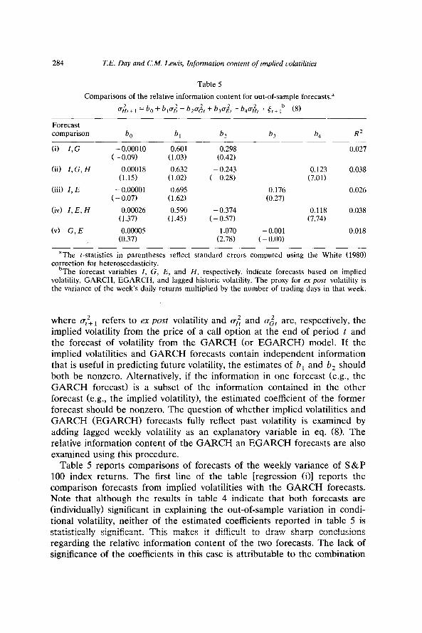
a~,+,=bo+b,~~+bbZ~~,+b3u~,+b4~~,+~,+,b (8)

Forecast comparison ba b, b, b, b, R2

6) I,G - 0.00010 ( - 0.09)

(ii) I,G, H 0.00018 (1.15)

(iii) I, E - 0.00001 ( - 0.07)

(iv) I, E, H 0.00026 (1.37)

(v) G, E 0.00005 (0.37)

0.601 (1.03)

0.632 (1.02)

0.695 (1.62)

0.590 (1.45)

0.298 (0.42)

- 0.243 (- 0.28)

- 0.374 ( - 0.57)

1.070 (2.78)

0.027

0.123 0.038 (7.01)

0.176 0.026 (0.27)

0.118 0.038 (7.74)

- 0.001 0.018 (- 0.00)

“The t-statistics in parentheses reflect standard errors computed using the White (1980) correction for heteroscedasticity.

bThe forecast variables I, G, E, and H, respectively, indicate forecasts based on implied volatility, GARCH, EGARCH, and lagged historic volatility. The proxy for ex post volatility is the variance of the week’s daily returns multiplied by the number of trading days in that week.

where a,!+, refers to ex post volatility and v,: and az2, are, respectively, the implied volatility from the price of a call option at the end of period t and the forecast of volatility from the GARCH (or EGARCH) model. If the implied volatilities and GARCH forecasts contain independent information that is useful in predicting future volatility, the estimates of b, and b, should both be nonzero. Alternatively, if the information in one forecast (e.g., the GARCH forecast) is a subset of the information contained in the other forecast (e.g., the implied volatility), the estimated coefficient of the former forecast should be nonzero. The question of whether implied volatilities and GARCH (EGARCH) forecasts fully reflect past volatility is examined by adding lagged weekly volatility as an explanatory variable in eq. (8). The relative information content of the GARCH an EGARCH forecasts are also examined using this procedure.

Table 5 reports comparisons of forecasts of the weekly variance of S&P 100 index returns. The first line of the table [regression (iI] reports the comparison forecasts from implied volatilities with the GARCH forecasts. Note that although the results in table 4 indicate that both forecasts are (individually) significant in explaining the out-of-sample variation in condi- tional volatility, neither of the estimated coefficients reported in table 5 is statistically significant. This makes it difficult to draw sharp conclusions regarding the relative information content of the two forecasts. The lack of significance of the coefficients in this case is attributable to the combination

T.E. Day and CM. Lewis, Information content of implied colatilities 285

of the large variance of the forecast error for the regression and to the relatively high correlation (0.71) of the implied volatilities with the GARCH forecasts. Note that regression (ii>, which includes lagged weekly volatility as an additional forecast, indicates that lagged historic volatility contains infor- mation which is not included in either the implied volatilities or the GARCH forecasts. Given the relatively small value of the coefficient for lagged volatility (b,), this result is probably attributable to a combination of instabil- ity of the parameters of the GARCH model and to model misspecification.

The comparisons for the EGARCH forecasts and implied volatility are similar to those for the GARCH forecasts. The third line of table 5 [regres- sion (iii)] shows that the estimated coefficients for the EGARCH forecast and the implied volatility are not statistically significant. The fact that the coeffi- cient of (b,) has a higher f-statistic than in regression (i> is likely due to the smaller correlation (0.49) between the EGARCH forecasts and the implied volatilities. In regression (iv), the coefficient for lagged volatility is small and statistically significant, and the coefficients for the EGARCH and implied volatility forecasts are insignificant. In fact, the results are very similar to regression (ii).

The final regression reported in table 5 compares the GARCH and EGARCH forecasts. The results show that the coefficient for the GARCH forecast (b,) is significantly greater than zero, while the coefficient for the EGARCH forecast (b,) is not significantly greater than zero. This indicates that for this sample period the EGARCH forecasts do not contain any information that is not contained in the GARCH forecasts. This conclusion is consistent with the results presented in table 4.

These out-of-sample forecast comparisons indicate that short-run market volatility is difficult to predict. Although the results are consistent with the hypothesis that both implied volatilities and GARCH models provide unbi- ased forecasts of weekly volatility, we are unable to make strong statements concerning the relative information content of GARCH forecasts and im- plied volatilities. However, the results do provide limited evidence that, in certain instances, GARCH models provide better forecasts than EGARCH models.

6. Conclusion

This paper examines the information content of the implied volatilities from call options on the S&P 100 index. Whereas previous studies of the information content of implied volatilities have used a cross-sectional regres- sion approach to infer information content, we examine information content relative to GARCH and Exponential GARCH models of conditional volatil- ity. Although the interpretation of the results is complicated by model misspecification and expiration day effects which add noise to the forecasts of

286 T.E. Day and C.M. Lewis, Information content of implied volatilities

future volatility implicit in option prices, the (within-sample) results suggest that implied volatilities may contain incremental information relative to the conditional volatility from GARCH and EGARCH models. We also find strong within-sample evidence that the conditional volatility estimates from GARCH and EGARCH models reflect incremental information relative to implied volatility. Taken together these results imply that neither implied volatility nor the conditional volatilities from GARCH and EGARCH models completely characterize within-sample conditional stock market volatility when the excess market return is assumed to be a linear function of conditional market volatility.

We explore this issue further by performing out-of-sample comparisons of the relative predictive power of the volatility forecasts to ex post volatility. These out-of-sample forecast comparisons indicate that weekly volatility is difficult to predict. Although the results are consistent with the hypothesis that implied volatility and the GARCH and EGARCH forecasts are unbi- ased, we are unable to make strong statements concerning the relative information content of GARCH forecasts and implied volatilities. However, the results provide limited evidence that, in certain instances, GARCH models provide better forecasts than EGARCH models.

References

Akgiray, Vedat, 1989, Conditional heteroscedasticity in time series of stock returns: Evidence and forecasts, Journal of Business 62, 55-80.

Beckers, Stan, 1981, Standard deviations implied in option prices as predictors of future stock price variability, Journal of Banking and Finance 5, 363-381.

Black, Fischer, 1976, Studies of stock price volatility changes, in: Proceedings of the 1976 meetings of the Business and Economic Statistics Section, American Statistical Association, 171-181.

Black, Fischer and Myron Scholes, 1973, The pricing of options and corporate liabilities, Journal of Political Economy 81, 637-659.

Bollerslev, Tim, 1986, Generalized autoregressive conditional heteroscedasticity, Journal of Econometrics 31, 307-327.

Bollerslev, Tim and Jeffrey M. Wooldridge, 1988, Quasi-maximum likelihood estimation of dynamic models with time-varying covariances, Unpublished manuscript.

Bollerslev, Tim, Robert F. Engle, and Jeffrey M. Wooldridge, 1988, A capital asset pricing model with time-varying covariances, Journal of Political Economy 96, 116-131.

Chiras, Donald P. and Steven Manaster, 1978, The information content of option prices and a test of market efficiency, Journal of Financial Economics 6, 213-234.

Christie, Andrew A., 1982, The stochastic behavior of common stock variances: Value, leverage and interest rate effects, Journal of Financial Economics 10, 407-432.

Day, Theodore E. and Craig M. Lewis, 1988, The behavior of the volatility implicit in the prices of stock index options, Journal of Financial Economics 22, 103-122.

Engle, Robert F., 1982, Autoregressive conditional heteroscedasticity with estimates of the variance of UK inflation, Econometrica 50, 987-1008.

Engle, Robert F., David M. Lilien, and Russell P. Robins, 1987, Estimating time varying risk premia in the term structure: The ARCH-M model, Econometrica 55, 391-407.

Fair, Ray C. and Robert J. Shiller, 1990, Comparing information in forecasts from econometric models, American Economic Review 80, 375-389.

T.E. Day and CM. Lewis, Information content of implied rolatilities 287

Feinstein, Steven P., 1989, A theoretical and empirical investigation of the Black-Scholes implied volatility, Dissertation (Yale University, New Haven, CT).

French, Kenneth R., G. William Schwert, and Robert F. Stambaugh, 1987, Expected stock returns and volatility, Journal of Financial Economics 19, 3-30.

Hull, John and Alan White, 1987, The pricing of options on assets with stochastic volatilities, Journal of Finance 42, 281-400.

Latane, Henry A. and Richard J. Rendleman, 1976, Standard deviations of stock price ratios implied in option prices, Journal of Finance 31, 369-381.

Lamoureux, Christopher B. and William D. Lastrapes, 1990, Forecasting stock return variance: Toward an understanding of stochastic implied volatilities, Unpublished manuscript.

Melino, Angelo and Stuart M. Turnbull, 1990, Pricing foreign currency options with stochastic volatility, Journal of Econometrics 45, 239-265.

Merton, Robert C., 1973, The theory of rational option pricing, Bell Journal of Economics and Management Science 4, 141-183.

Merton, Robert C., 1980, On estimating the expected return on the market: An exploratory investigation, Journal of Financial Economics 8, 323-361.

Nelson, Daniel B., 1988, Conditional heteroscedasticity in asset returns: A new approach, Unpublished manuscript (University of Chicago, Chicago, IL).

Nelson, Daniel B., 1990, ARCH models as diffusion approximations, Journal of Econometrics 45, 7-38.

Officer, Robert R., 1973, The variability of the market factor of New York Stock Exchange, Journal of Business 46, 434-453.

Pagan, Adrian R. and G. William Schwert, 1990, Alternative models for conditional stock volatility, Journal of Econometrics 45, 267-290.

Poterba, James M. and Lawrence H. Summers, 1986, The persistence of volatility and stock market fluctuations, American Economic Review 76, 1142-1151.

Schwert, G. William, 1989, Why does stock market volatility change over time?, Journal of Finance 44, 1115-1153.

Schwert, G. William, 1990. Stock volatility and the crash of ‘87, Review of Financial Studies 3, 77-102.

Scott, Louis O., 1987, Option pricing when the variance changes randomly: Theory, estimation and an application, Journal of Financial and Quantitative Analysis 22, 419-438.

Whaley, Robert E., 1982, Valuation of American call options on dividend-paying stocks: Empirical tests, Journal of Financial Economics 10, 29-58.

White, Halbert, 1980, A heteroscedasticity-consistent covariance matrix estimator and a direct test for heteroscedasticity, Econometrica 48, 817-838.

Wiggins, James B., 1987, Option values under stochastic volatility: Theory and empirical estimates, Journal of Financial Economics 19, 351-372.