Embed Size (px)
Citation preview
ICES Stock Annex | 1
Stock Annex: Southern Sardine stock Annex (Divisions 8.c and 9.a)
Stock-specific documentation of standard assessment procedures used by the Interna-tional Council for Exploration of the Sea (ICES).
Stock: Sardine (Sardina pilchardus) in divisions 8.c and 9.a (Cantabrian Sea and Atlantic Iberian waters)
Working group: Working Group on Anchovy and Sardine and Southern Horse Macke-rel (WGHANSA)
Revised by: WKPELA2017
Main modifications: Information on stock delimitation and the description of the fish-eries were updated based on recent studies (e.g. ICES, 2016a; Silva et al., 2015). The main modifications of the assessment regard the methods to estimate the initial popu-lation, the stock-recruitment relationship, the acoustic survey selectivity-at-age and the fishery selectivity-at-age (ICES, 2017a).
Last updated: March 2017
Last Benchmarked: February 2017
Authors: Alexandra Silva, Pablo Carrera Isabel Riveiro, Cristina Nunes, Laura Wise, and the members of WKPELA
A.3.1 Stock definition
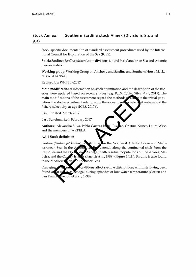
Sardine (Sardina pilchardus) is distributed in the Northeast Atlantic Ocean and Medi-terranean Sea. In the Atlantic, sardine extends along the continental shelf from the Celtic Sea and the North Sea to Senegal, with residual populations off the Azores, Ma-deira, and the Canary Islands (Parrish et al., 1989) (Figure 3.1.1.). Sardine is also found in the Mediterranean and the Black Seas.
Changing environmental conditions affect sardine distribution, with fish having been found as far south as Senegal during episodes of low water temperature (Corten and van Kamp, 1996; Binet et al., 1998). REPLA
CED
2 | ICES Stock Annex
Figure A.1.1. Geographical distribution of European sardine.
Two stocks are considered in EU Atlantic waters: Northern stock (ICES Subareas 7 and 8.a,b,d) fished mainly by France and Spain, and Southern stock (ICES Subarea 8.c and Division 9.a) fished by Spain and Portugal (Figure A.1.2).
Figure A.1.2. Delimitation of the Southern sardine stock (divisions 8.c and 9.a).
REPLACED
ICES Stock Annex | 3
There is no evidence to support a change of the current stock boundaries. There is no indication of strong demographic connectivity between the two stocks. However, lo-cally there are signs of regional substructure and potentially different population dy-namics (especially for areas in the limits, as the Gulf of Cadiz), revealed through multidisciplinary studies (see ICES, 2016a):
• Genetic studies, using different molecular markers are not fully consistent; ear-lier studies using allozymes and studies using mtDNA indicated a higher de-gree of differentiation than recent studies using allozymes and studies using microsatellite DNA. In general, no genetic structure is evident in most of the distribution range for neutral markers and genetic differenciation among indi-viduals increases as geographical distance increases (Kasapidis, 2014).
• Data on cohort dynamics in recent years, when recruitment was high in the Bay of Biscay and low in the Iberian area, do not indicate massive straying of cohorts from the Bay of Biscay to the Cantabrian Sea or further south. This suggests the dynamics of the Southern stock is not significantly affected by the dynamics of the Northern stock.
• Growthpattern by regions suggest some heterogeneity among the northern re-gions, with larger homogeneity in the periods 2000–2010 than in the years 2011–2016, whereby in Biscay smaller sardine mean growth than in the Canta-brian regions are seen.
• The continuity of the spawning area, overlap in spawning seasons, similarity of genetic, morphometric and life-history properties studied in SARDYN pro-ject (2002–2005) support mixing between the stocks (Anon, 2006). Trial area-based assessments with different models indicated that migrations, most likely involving a net immigration from Biscay to Cantabria, were plausible.Further work after SARDYN with the Bayesian state–space model estimated likely em-igration from south Biscay (8.b) to east Cantabria (8.c-east) for 1-year-olds and also estimated likely immigration (at a smaller rate) into east Cantabria for 2+ adults (ICES, 2006). However, the total-stock biomass in Iberia resulting from immigration from Biscay was estimated to be low (1–4%).
• There is there evidence of connectivity between Cantabrian/North Galicia and western Portugal, both at both at the larval and adult stages. Marked geo-graphical differences in adult growth patterns places south Galicia in an inter-mediate region between the high growth levels of sardine in the northern regions (North Galicia and Cantabria) and the smaller growth levels observed in the western Portuguese areas. In a recent study, using a biophysical model for simulating early life stages of sardine, Garcia-Garcia et al. (2016) observed an alongshore transport of larvae spawned in Portugal to the Cantabrian sea and vice-versa. They argue that the transport from Cantabria to north Portugal may be more important as a connectivity process because while larvae trans-ported to the Cantabrian Sea end up in a cold area with limited food, some-times larvae transported to the northern Portuguese shelf from the Cantabrian Sea end up in a favourable environment.
• Data on otolith microchemistry and cohort dynamics support the hypothesis that sardine cohorts stray from western Iberian to North Galicia and the Can-tabrian Sea during their first 2–3 years of life.
• Growth patterns suggest some partially independent dynamics between the northern areas and the western areas. But higher lengths-at-age in northern areas might also suggest straying of larger fish to the north.
REPLACED
4 | ICES Stock Annex
• However, sardine body and otolith shape, life-history properties and cohort dynamics, all point to some differentiation between the western and the south-ern areas, mainly with respect to the Gulf of Cadiz. In terms of otolith shape, growth and maturation sardine distributed in the Gulf of Cadiz appear to be closer to sardine in southwestern Mediterranean than to those in western Por-tugal.
• Areas in the limits, Gulf of Cadiz and Channel/North Sea, show differentiation in some approaches (Gulf of Cadiz: otolith shape, morphometrics, recruitment dynamics / English Channel: otolith shape, growth) but further information from the area (in the case of Channel/Celtic Sea/ North Sea) or from adjacent areas (Southwestern Mediterranean and northern Morocco) is needed.
A.3.2 Fishery
General description
The bulk of the landings in both Spain and Portugal (99%) are made by purse-seiners (e.g. Silva et al., 2015).
The Spanish purse seine fleet targets anchovy (Engraulis encrasicolus), mackerel (Scomber scombrus) and sardine, (which occur seasonally in the area) and horse-macke-rel (Trachurus trachurus) which is available all year-round (Uriarte et al., 1996; Villamor et al., 1997; Carrera and Porteiro, 2003). In summer, part of the fleet switches to trolling lines or bait boat for tuna fishing, a resource with a marked seasonal character. Since 2004, Spanish legislation requires that purse seiners must have, at least, a length of 11 m in the Atlantic coast of Spain. Moreover, the gear must have a maximum length of 600 m, a maximum height of 130 m and minimum mesh size of 14 mm. Because of this regulation, most of the effort and catches are registered in logbooks (which are man-datory for boats larger than 10 m). Analysis of these logbook data from 2003 to 2005 (Abad et al., 2008) showed that sardine and horse-mackerel represent 75% of the total landings of the purse seine fleet, which is in accordance with the values observed in historical series of purse seine catch statistics, especially when the anchovy is scarce (ICES, 2007). Sardine catches show the highest values in summer and autumn and ef-fort concentrates in southern Galician and western Bay of Biscay waters. Vessels can be characterized by 21 m length overall, 292 HP, and 56 gross tonnage.
In Portugal, sardine is the main target species of the purse seine fleet comprising 98% of the landings. The sardine fishery is of great social-economical importance for the fishing community and industry since it represents an important part of the fish pro-duction and a relevant supply for the canning sector. Other pelagic species such as chub mackerel (Scomberjaponicus), horse mackerel and anchovy are also landed by the purse seine fishery. Currently, purse seiners in Portuguese waters have a length of about 20 m, an engine horsepower between 100 and 500 HP and use a minimum mesh size of 16 mm. Fishing is usually close to the home port, on short (daily) trips where the net is set once or twice, usually around dawn (Stratoudakis and Marçalo, 2002). A large part of a typical fishing trip is spent searching for schools with echosounders and sonars. Once schools of pelagic fish have been detected, large nets (up to 800 m long and 150 m deep) are set rapidly with the help of an auxiliary small vessel, and hauled in a largely manual operation involving all members of the crew (usually between 15–20 people) (Mesquita, 2008).
Fishery management regulations
Regulation measures in both Spain and Portugal for purse-seine fishery include mini-mum landing sizes, specifications for design and use of gears, minimum mesh sizes for
REPLACED
ICES Stock Annex | 5
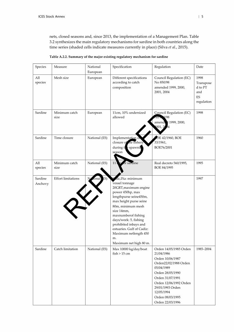
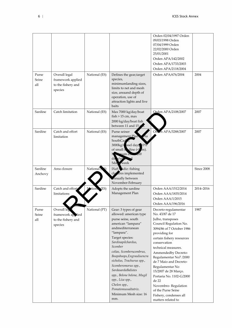
nets, closed seasons and, since 2013, the implementation of a Management Plan. Table 3.2 synthesizes the main regulatory mechanisms for sardine in both countries along the time series (shaded cells indicate measures currently in place) (Silva et al., 2015).
Table A.2.2. Summary of the major existing regulatory mechanism for sardine
Species Measure National European
Specification Regulation Date
All species
Mesh size European Different specifications according to catch composition
Council Regulation (EC) No 850/98 amended 1999, 2000, 2001, 2004
1998 Transposed to PT and ES regulation
Sardine
Minimum catch size
European 11cm, 10% undersized allowed
Council Regulation (EC) No 850/98 amended 1999, 2000, 2001, 2004
1998
Sardine
Time closure National (ES)
Implementation of a closure of the fishery during the spawning season
BOE 42/1960, BOE 33/1961, BOE76/2001
1960
All species
Minimum catch size
National (ES) 11 cm for sardine Real decreto 560/1995, BOE 84/1995
1995
Sardine Anchovy
Effort limitations National (ES)
VIIIc,IXa: minimum vessel tonnage 20GRT,maximum engine power 450hp, max lengthpurse seine450m, max height purse seine 80m, minimum mesh size 14mm, maxnumberof fishing days/week: 5, fishing prohibited inbays and estuaries. Gulf of Cadiz: Maximum netlength 450 m. Maximum net high 80 m.
1997
Sardine
Catch limitation National (ES) Max 10000 kg/day/boat fish > 15 cm
Orden 14/05/1985 Orden 21/04/1986 Orden 10/06/1987 Orden22/02/1988 Orden 05/04/1989 Orden 28/05/1990 Orden 31/07/1991 Orden 12/06/1992 Orden 29/01/1993 Orden 12/05/1994 Orden 08/03/1995 Orden 22/03/1996
1985–2004
REPLACED
6 | ICES Stock Annex
Orden 02/04/1997 Orden 09/03/1998 Orden 07/04/1999 Orden 22/02/2000 Orden 25/01/2001 Orden APA/142/2002 Orden APA/1733/2003 Orden APA/2118/2004
Purse Seine all
Overall legal framework applied to the fishery and species
National (ES)
Defines the gear,target species, minimumlanding sizes, limits to net and mesh size, areaand depth of operation, use of attraction lights and live baits
Orden APA/676/2004 2004
Sardine
Catch limitation National (ES) Max 7000 kg/day/boat fish > 15 cm, max 2000 kg/day/boat fish between 11 and 15 cm.
Orden APA/2108/2007 2007
Sardine
Catch and effort limitation
National (ES)
Purse seiner management Plan in IXa SouthCadiz: 3000kg/vessel day(<10% of small sardine (<9cm). Maximum effort 200 days/year and 5days/week
Orden APA/3288/2007 2007
Sardine Anchovy
Area closure National (ES)
IXaS Cádiz: fishing closures implemented annually between November-February
Since 2008
Sardine
Catch and effort limitations
National (ES)
Adopts the sardine Management Plan
Orden AAA/1512/2014 Orden AAA/1835/2014 Orden AAA/1/2015 Orden AAA/196/2016
2014–2016
Purse Seine all
Overall legal framework applied to the fishery and species
National (PT)
Gear: 3 types of gear allowed: american type purse seine, south american “lampara” andmediterranean “lampara”. Target species: Sardinapilchardus, Scomber colias, Scomberscombrus, Boopsboops,Engraulisencrasicholus, Trachurus spp., Scomberomorus spp., SardasardaBalistes spp., Belone belone, Mugil spp., Liza spp., Chelon spp., Pomatomussaltatrix. Minimum Mesh size: 16 mm.
Decreto-regulamentar No. 43/87 de 17 Julho, transposes Council Regulation No. 3094/86 of 7 October 1986 providing for certain fishery resources conservation technical measures. Ammendedby Decreto-Regulamentar No7 /2000 de 7 Maio and Decreto- Regulamentar No 15/2007 de 28 Março. Portaria No. 1102-G/2000 de 22 Novembro- Regulation of the Purse Seine Fishery, condenses all matters related to
1987 REPLACED
ICES Stock Annex | 7
Minimum Landing Size: 11 cm. Limits to net size: variable with vessel LOA,maximum length 800 m, maximum height 150m. Attraction lights: at most two attraction lightsin areas over 2 miles distance of the coastline. Area and depth of operation: within ¼ milesdistance to the coastline, as well as, in depthsbelow 20 m within 1 mile distance to thecoastline.
fishing with purse seine from the previous regulations. AmmendedbyPortaria No.346/2002,de 2 de Abril and Portaria No. 397/2007 de 4 de Abril.
Purse Seine Sardine
Effort limitation Time/area closure
National (PT)
Limits the number of fishing days per year (lower in the north) and per week (5 days), seasonal fishing closures winter/spring in thenorthern coast. 10% by-catch allowed in otherfisheries.
Portarian.o 281-B/97 de 30 de Abril
1997
Purse seine Sardine
Effort and catch limitations
National (PT)
Reduces the number of fishing days per year and equal along the coast, sets annual catchlimits, split by POs in some years, sets quotafor non-associated vessels. 10% by-catchallowed in other fisheries.
Portaria nº 236/2000 de 28 de Abril,Portaria No. 543-B/2001 de 30 Maio,Portaria No. 123-A/2002 de 8 Fevereio, Portaria No. 184/2003 de 21 Fevereiro,Portarian.o 1423- A/2003 de 31 Dezembro
2000–2004
Purse Seine Sardine
Catch limitations National (PT)
Maximum catch: 55 000 tonnes in 2010 and 2011 Maximum fishing days per year (180 days) andper week (5 days) Crates a consultative Commission of stakeholders for the sardine fishery coordinated by the Fisheries Management Authority
Portaria n.º 251/2010 de 4 Maio, Portaria n.º 294/2011, de 14 de Novembro.
2010–2011
Purse Seine Sardine
Catch and effort limitations
National (PT)
Adopts the sardine Management Plan. Catch limits set for successive periods alongthe year. Annual limits 36 000 tonnes in 2012,2013, 13 500
Despacho n.º 1520/2012, de 18 de janeiro, Despacho n.º 7509/2012, de 29 de maio, Despacho n.º 15351-A/2012, de
2012–2014
REPLACED
8 | ICES Stock Annex
tonnessin 2014. Portugueselandings assumed to be 70% of total stocklandings. 45 day fishing ban in winter/spring alternatingbetween regions.
30 de novembro, Despacho n.º 12213/2013 de 25 de setembro,Despacho n.º 7112-A/2013 31 de maio,Despacho n.º 15261/2013 22 de novembro, Despacho n.º 8503/2014 1 de julho, Despacho n.º 8856/2014 9 dejulho
Purse Seine Sardine
Time closure Effort and catch limitations
National (PT)
59 days fishing ban in winter/spring A single trip per day. Maximum catch per vessel per day dependingon vessel LOA. Maximum 6 tonnes/day forLOA> 16 m. Catch limits set by period: total in year 13 500tonnes. Catches split by PO. Portuguese landings assumed to be 68% of total stock landings. Specific limits for sardine in commercial category T4 (36-67 individuals/Kg)
Despacho n.º 15793-B/2014 31 de dezembro, Despacho n.º 2179-A/2015 de 2 Março, Despacho n.º 5119-H/2015 15 demaio.
2015
Sardine
Catch limitation small individuals
National (PT)
No catch of sardine T4 Despacho n.º 10062-B/2015 de 4 de setembro
Since 04/09/2015
A.3.3 Ecosystem aspects
Sardine distribution is restricted to coastal shelf waters, mainly at depth above 150 m, forming dense schools during daytime. Sardine shows a preference for waters with low temperature and salinity, high chlorophyll content and low planktonic backscat-tering energy (Zwolinski et al., 2008).
Sardine feeds mainly on zooplankton (mainly copepods; Bode et al., 2004; Costalago et al., 2012; Jemaa et al., 2015), and may also have alternative preys such as phytoplankton. In addition, sardines have been found to ingest their own eggs (and probably those of other species) and this cannibalism may act as a density control mechanism (Garrido et al., 2007, 2015).
Above a size threshold (around 4 cm), sardine can change from filter feeding to partic-ulate feeding depending on the relative abundance of these prey groups (Varela et al., 1988; Bode et al., 2003; Garrido et al., 2007; Costalago and Palomera, 2014). This strategy can be useful during periods of low food availability, even though sardine has demon-strated to have a less flexible diet than other pelagic fishes, such as anchovy (Chouvelon et al., 2014; 2015, Costalago and Palomera 2014). This confers a competitive disadvantage to the sardine and leads to a segregation of both species in terms of or-ganisms preyed and feeding areas.
REPLACED
ICES Stock Annex | 9
Sardine can be considered a “forage species” because is a small sized organism that serves as food for many marine predators which take advantage of its schooling be-haviour and availability, including mammals (Thompson et al., 1996; Silva, 2001; Weise and Harvey 2008; Santos et al., 2013), seabirds (Crawford and Dyer 1995; Jahncke et al., 2004; Furness and Edwards 2007; Daunt et al., 2008) and larger fish species (Walter and Austin 2003; Magnussen 2011). Forage fish are important for energy transfer through the pelagic food web, and some species have demonstrated to exert a “waspwaist” control, especially in upwelling ecosystems: they exert both (top down) control of zo-oplankton and (bottom up) control of top predators (Rice, 1995; Cury et al., 2000).
Sardine has been found to be important in the diet of common dolphins (Delphinusdel-phis)in Galicia (NW Spain) Portugal (Silva, 2001) and the Atlantic French coast (Mey-nier, 2004),but recent studies (Santos et al., 2014) indicate that cetacean predation on sardinerepresents only 2–8% of the total natural mortality rate, with little influence on sardinepopulation dynamics.There are also other species feeding on sardine,although to a lesser extent, such asharbour porpoise (Phocoenaphocoena), bottlenose dolphin (Tur-siopstruncatus), striped dolphin (Stenellacoeruleoalba), and white-sided dolphin (Lagen-orhynchusacutus) (e.g. Santos et al., 2007).
As many other pelagic species, sardine, due to a high dependency of lower trophic levels (Costalago and Palomera 2014), can be highly vulnerable to changes in environ-mental conditions and plankton community. Sardine abundance, biomass and distri-bution show important fluctuations in different ecosystems all around the world in response to environmental variability and climate change (Carrera and Porteiro, 2003; Alheit et al., 2014). Shifts in global atmospheric and sea temperatures coincide with productivity cycles, but the mechanistic link may be caused by an associated process operating at regional level (Lluch-Belda et al., 1992). The relationship between popula-tion characteristics and environmental variables is therefore complex, depending on the temporal scale and varying across regions, due to the different recruitment re-sponses in the different areas studied (Guisande et al., 2001; Santos et al., 2012; Leitao et al., 2014).
Changes in sardine biomass are tightly coupled to the magnitude of recruitment. In turn, recruitment is mainly dependent on environmental conditions, such as tempera-ture and productivity (Santos et al., 2001, 2005; Guisande et al., 2004; Santos et al., 2012). Fishing may amplify recruitment fluctuations and in extreme situations lead to recruit-mentoverfishing.
A.3.4 Data
A.3.4.1 Commercial catch
Landings data
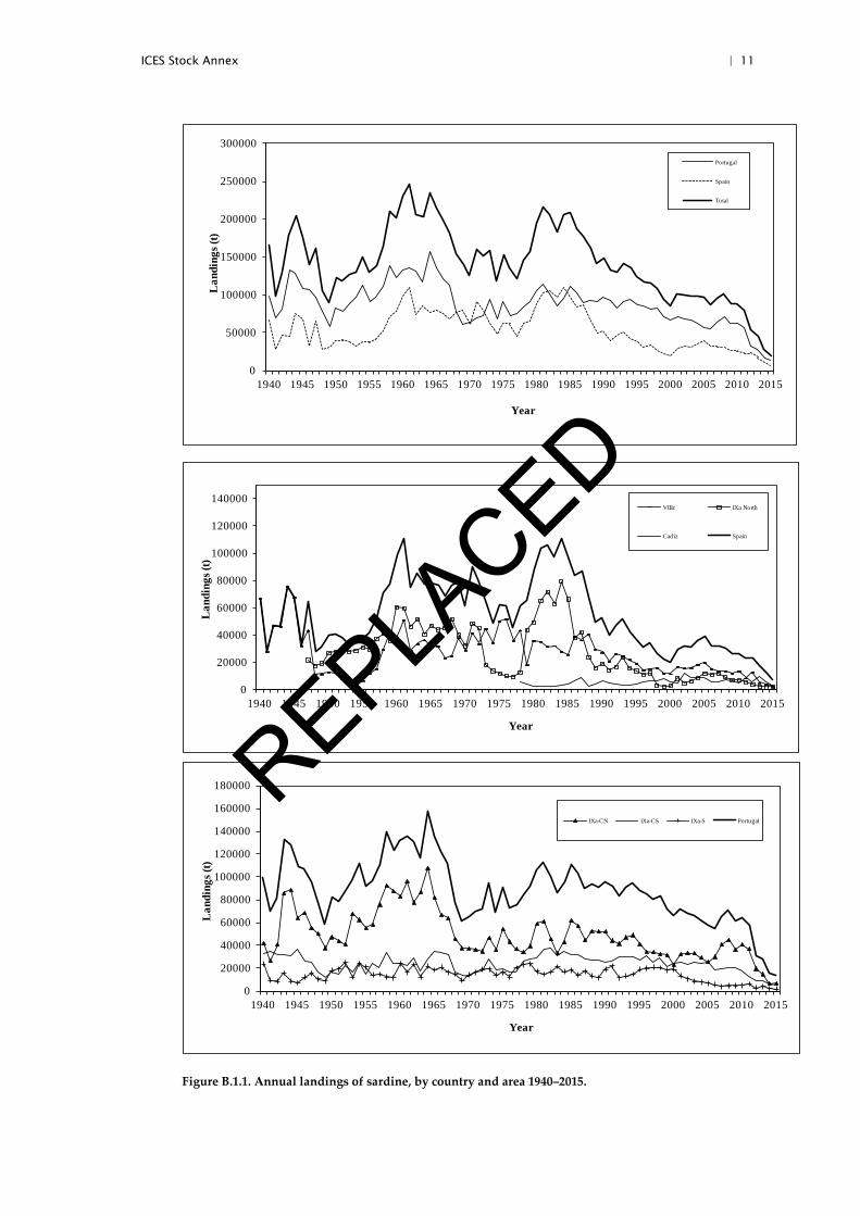
Commercial catch data are obtained from the national laboratories of both Spain and Portugal. Annual landings are available since 1940 (see Figure B.1). Landings are not considered to be significantly under reported.
Landingsdata are collected by the Spanish and Portuguese government official entities responsible for fisheries data (Secretaría General de Pesca Iin Spain, General Fisheries Directorate in Portugal) and cover the whole assessment period (since 1978) and the whole stock area. Landings are considered to be unbiased and precise.
Up to 1990, landings were reported by three stock areas (Spain–8.c, Spain–9.a, and Por-tugal–9.a). Since 1991, both Spanish and Portuguese labs have used a common format to provide all necessary landing and sampling data by quarter and disaggregated in
REPLACED

10 | ICES Stock Annex
seven sub-areas (8.c.e, 8.c.w, 9.a.n, 9.a.c.n, 9.a.c.s, 9.a.s.a and 9.a.s.c). It should be noted that only sampled, official, WG catch are available in this file.
Commercial catch and sampling data are stored and processed using the INTER-CATCH.
REPLACED
ICES Stock Annex | 11
Figure B.1.1. Annual landings of sardine, by country and area 1940–2015.
0
50000
100000
150000
200000
250000
300000
1940 1945 1950 1955 1960 1965 1970 1975 1980 1985 1990 1995 2000 2005 2010 2015
Lan
ding
s (t)
Year
Portugal
Spain
Total
0
20000
40000
60000
80000
100000
120000
140000
1940 1945 1950 1955 1960 1965 1970 1975 1980 1985 1990 1995 2000 2005 2010 2015
Lan
ding
s (t)
Year
VIIIc IXa North
Cadiz Spain
0
20000
40000
60000
80000
100000
120000
140000
160000
180000
1940 1945 1950 1955 1960 1965 1970 1975 1980 1985 1990 1995 2000 2005 2010 2015
Lan
ding
s (t)
Year
IXa-CN IXa-CS IXa-S Portugal
REPLACED
12 | ICES Stock Annex
Discards estimates
Total discards, including slipping, are not available for the fishery.
Recent data from on board observers in Portugal (Fernandes and Feijó, 2016WD, Feijó, 2013) and Spanish regular DCF monitoring in 2015, show that discards of fish after hauling the catch aboard (whereby all fish die) are negligible and do not constitute a major issue for this fishery. Sardine constituted 97% of the landings in the trips ob-served and >99% of the total for the whole fleet, and some of the bycatch species caught in small quantities during the trips observed never reached the market.
Total discards are very difficult to measure. As with other pelagic fisheries that exploit schooling fish discarding occurs in a sporadic way and with often extreme fluctuation in discard rates (100% or null discards). Extreme discards occur especially when the entire catch is released after the drying-up ofthe net but without the fish being drawn aboard (slipping). Slipping tends to be related to quota limitations, illegal size and mix-ture with unmarketable bycatch (Stratoudakis and Marçalo, 2002; Marçalo, 2009). Quantifying such discards at a population level is extremely difficult because they vary considerably between years, seasons, species targeted and geographical region. In ad-dition, mortality of slipped fish is also highly variable and has not been evaluated at sea (e.g. Marçalo, 2009)
A.3.4.2 Biological sampling
Maturity
Maturity ogive from the stock comes from DEPM surveys (ICES, 2017a).
• For years with no DEPM survey a linear interpolation of the data between two consecutive surveys was carried out to obtain the estimates of maturity at age.
• For the period 1978–1998 (years before starting DEPM series), constant pro-portions of maturity at age were assumed, based on the average of the esti-mates obtained from the 6 DEPM surveys of the 1999–2014 period, thus including both years of strong year classes and years of low recruitment.
• For the years after the last DEPM survey, the estimates of the last DEPM survey are assumed.
Natural mortality
Natural mortality are age specific input values as listed in the table below (ICES, 2017a).
Age Value, year-1
Age 0 0.98
Age 1 0.61
Age 2 0.47
Age 3 0.40
Age 4 0.36
Age 5 0.35
Age 6+
0.32
REPLACED
ICES Stock Annex | 13
Length, weight and age composition of landed and discarded fish in commercial fisheries
Catch-at-age data (catch numbers-at-age, mean weights-at-age in the catch, mean length-at-age) are derived from the raised national figures routinely provided by both Spain and Portugal. These data are obtained either by market sampling or by on board observers. In Spain, samples for age length keys are pooled on a half year basis for each subdivision while length/weight relationships are calculated quarterly. In Portugal, both age length keys and length/weight relationships are compiled on a quarterly and subdivision basis. Catch-at-age data are not available for the Gulf of Cadiz (sub-divi-sion 9.a.s.c) until 1998. For the period 1978–1997, catches-at-age for the Gulf of Cadiz are calculated applying the age composition of South Portugal to Cadiz landings. Since 1991 sampling design is stratified into seven geographical areas covering the whole stock (see Section B.1.1) and is considered unbiased and precise. Documentation on sampling design/intensity and allocation of length/age samples is not easily available prior to 1992.
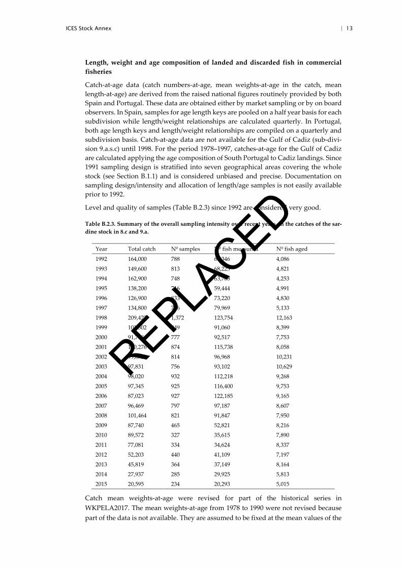
Level and quality of samples (Table B.2.3) since 1992 are considered very good.
Table B.2.3. Summary of the overall sampling intensity over recent years on the catches of the sar-dine stock in 8.c and 9.a.
Year Total catch Nº samples Nº fish measured Nº fish aged
1992 164,000 788 66,346 4,086
1993 149,600 813 68,225 4,821
1994 162,900 748 63,788 4,253
1995 138,200 716 59,444 4,991
1996 126,900 833 73,220 4,830
1997 134,800 796 79,969 5,133
1998 209,422 1,372 123,754 12,163
1999 101,302 849 91,060 8,399
2000 91,718 777 92,517 7,753
2001 110,276 874 115,738 8,058
2002 99,673 814 96,968 10,231
2003 97,831 756 93,102 10,629
2004 98,020 932 112,218 9,268
2005 97,345 925 116,400 9,753
2006 87,023 927 122,185 9,165
2007 96,469 797 97,187 8,607
2008 101,464 821 91,847 7,950
2009 87,740 465 52,821 8,216
2010 89,572 327 35,615 7,890
2011 77,081 334 34,624 8,337
2012 52,203 440 41,109 7,197
2013 45,819 364 37,149 8,164
2014 27,937 285 29,925 5,813
2015 20,595 234 20,293 5,015
Catch mean weights-at-age were revised for part of the historical series in WKPELA2017. The mean weights-at-age from 1978 to 1990 were not revised because part of the data is not available. They are assumed to be fixed at the mean values of the
REPLACED
14 | ICES Stock Annex
period 1991–1995. The mean weights-at-age for 1991 to 2015 were re-calculated using quarter and area disaggregated data reported to the assessment WGs every year by Spain and Portugal. The method adopted to calculate catch mean weights-at-age is the following: mean weights-at-age by quarter and area are aggregated to the quarter and then to the year using the corresponding catch numbers-at-age as weighting factors (this weighting had not been properly done before 1999).
Weights at age of the stock
Mean weights-at-age in the stock comes from DEPM surveys (ICES, 2017a).
• For years with no DEPM survey, a linear interpolation of the data from two consecutive surveys was carried out to obtain the estimates of mean weight at age.
• For the period 1978–1998 (before DEPM series started) it was decided to con-sider the two closest DEPM surveys, and assume for that period the average between 1999 and 2002 estimates.
• For the years after the last DEPM survey, the estimates of the last DEPM survey are assumed.
A.3.4.3 Surveys
Survey design and analysis
A.3.4.3.1. DEPM surveys
The Daily Egg Production Method started being applied to sardine in the Iberian Pen-insula during the 80s but surveys were interrupted for almost 10 years. Current DEPM surveys started in 1997 for both Spain and Portugal and have been carried out trienni-ally since 1999. Since 2002, the surveys have been conducted within the framework of ICES, with co-financing from the EU, on a triennial basis. Collaborative work between Portugal (IPMA) and Spain (IEO) over the years, led to increased coordination of the surveys and standardisation of surveying and analysis methodologies, and many de-velopments have been achieved under the auspices of the ICES groups SGSBSA (Study Group on the Estimation of Spawning Stock Biomass of Sardine and Anchovy) and WGACEGG (Working Group on Acoustics and Egg Surveys for Sardine and Anchovy in ICES Areas 7, 8 and 9). DEPM estimates of sardine SSB were last revised in Novem-ber 2016 (ICES 2017a,b).
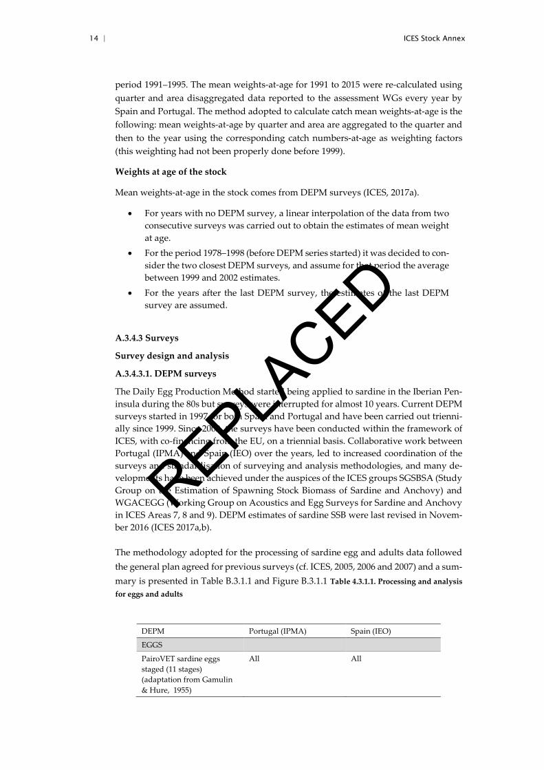
The methodology adopted for the processing of sardine egg and adults data followed the general plan agreed for previous surveys (cf. ICES, 2005, 2006 and 2007) and a sum-mary is presented in Table B.3.1.1 and Figure B.3.1.1 Table 4.3.1.1. Processing and analysis for eggs and adults
DEPM Portugal (IPMA) Spain (IEO)
EGGS
PairoVET sardine eggs staged (11 stages) (adaptation from Gamulin & Hure, 1955)
All All
REPLACED
ICES Stock Annex | 15
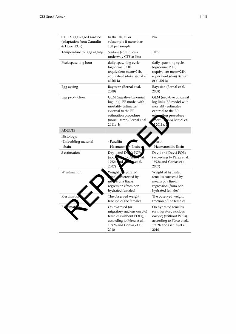
CUFES egg staged sardine (adaptation from Gamulin & Hure, 1955)
In the lab, all or subsample if more than 100 per sample
No
Temperature for egg ageing Surface (continuous underway CTF at 3m)
10m
Peak spawning hour daily spawning cycle, lognormal PDF, (equivalent mean=21h, equivalent sd=4) Bernal et al 2011a
daily spawning cycle, lognormal PDF, (equivalent mean=21h, equivalent sd=4) Bernal et al 2011a
Egg ageing Bayesian (Bernal et al. 2008)
Bayesian (Bernal et al. 2008)
Egg production GLM (negative binomial log link) EP model with mortality estimates external to the EP estimation procedure (mort ~ temp) Bernal et al 2011a, b
GLM (negative binomial log link) EP model with mortality estimates external to the EP estimation procedure (mort ~ temp) Bernal et al 2011a, b
ADULTS
Histology: -Embedding material - Stain
- Paraffin - Haematoxilin-Eosin
- Resin - Haematoxilin-Eosin
S estimation Day 1 and Day 2 POFs (according to Pérez et al. 1992a and Ganias et al. 2007)
Day 1 and Day 2 POFs (according to Pérez et al. 1992a and Ganias et al. 2007)
W estimation Weight of hydrated females corrected by means of a linear regression (from non-hydrated females)
Weight of hydrated females corrected by means of a linear regression (from non-hydrated females)
R estimation The observed weight fraction of the females
The observed weight fraction of the females
F estimation On hydrated (or migratory nucleus oocyte) females (without POFs), according to Pérez et al., 1992b and Ganias et al. 2010
On hydrated females (or migratory nucleus oocyte) (without POFs), according to Pérez et al., 1992b and Ganias et al. 2010
REPLACED
16 | ICES Stock Annex
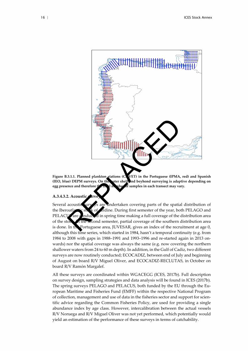
Figure B.3.1.1. Planned plankton stations (CalVET) in the Portuguese (IPMA, red) and Spanish (IEO, blue) DEPM surveys. On the outer shelf and beyhond surveying is adaptive depending on egg presence and therefore the final number of samples in each transect may vary.
A.3.4.3.2. Acoustic surveys
Several acoustic surveys are undertaken covering parts of the spatial distribution of the Iberoatlantic stock of sardine. During first semester of the year, both PELAGO and PELACUS are conducted in spring time making a full coverage of the distribution area of the stock. In the second semester, partial coverage of the southern distribution area is done. In the Portuguese area, JUVESAR, gives an index of the recruitment at age 0, although this time series, which started in 1984, hasn’t a temporal continuity (e.g. from 1984 to 2008 with gaps in 1988–1991 and 1993–1996 and re-started again in 2013 on-wards) nor the spatial coverage was always the same (e.g. now covering the northern shallower waters from 24 to 60 m depth). In addition, in the Gulf of Cadiz, two different surveys are now routinely conducted; ECOCADIZ, between end of July and beginning of August on board R/V Miguel Oliver, and ECOCADIZ-RECLUTAS, in October on board R/V Ramón Margalef.
All these surveys are coordinated within WGACEGG (ICES, 2017b). Full description on survey design, sampling strategies and data analysis will be found in ICES (2017b). The spring surveys PELAGO and PELACUS, both funded by the EU through the Eu-ropean Maritime and Fisheries Fund (EMFF) within the respective National Program of collection, management and use of data in the fisheries sector and support for scien-tific advice regarding the Common Fisheries Policy, are used for providing a single abundance index by age class. However, intercalibration between the actual vessels R/V Noruega and R/V Miguel Oliver was not yet performed, which potentially would yield an estimation of the performance of these surveys in terms of catchability.
REPLACED
ICES Stock Annex | 17
Outside the assessed stock area, the spring acoustic survey PELGAS (run by IFREMER) covers the area from the south of the Bay of Biscay to south of Brittany.
Portuguese Spring acoustic survey: PELAGO
The Portuguese acoustic surveys (onboard the RV “Noruega”) are mainly directed to sardine and anchovy.
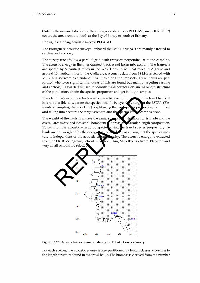
The survey track follow a parallel grid, with transects perpendicular to the coastline. The acoustic energy in the inter-transect track is not taken into account. The transects are spaced by 8 nautical miles in the West Coast, 6 nautical miles in Algarve and around 10 nautical miles in the Cadiz area. Acoustic data from 38 kHz is stored with MOVIES+ software as standard HAC files along the transects. Trawl hauls are per-formed whenever significant amounts of fish are found but mainly targeting sardine and anchovy. Trawl data is used to identify the echotraces, obtain the length structure of the population, obtain the species proportion and get biologic samples.
The identification of the echo traces is made by eye, with the aid of the trawl hauls. If it is not possible to separate the species schools by eye, the energy of the ESDUs (Ele-mentary Sampling Distance Unit) is split using the haul species proportion, in number, and taking into account the target strength and the species length compositions.
The weight of the hauls is always the same, since a post stratification is made and the overall area is divided into small homogeneous areas, with similar length composition. To partition the acoustic energy by species, using the trawl species proportion, the hauls are not weighted by the energy around the haul, assuming that the species mix-ture is independent of the acoustic energy density. The acoustic energy is extracted from the EK500 echograms, school by school, using MOVIES+ software. Plankton and very small schools are rejected.
Figure B.3.2.1. Acoustic transects sampled during the PELAGO acoustic survey.
For each species, the acoustic energy is also partitioned by length classes according to the length structure found in the trawl hauls. The biomass is derived from the number
REPLACED
18 | ICES Stock Annex
of individuals, applying the weight/length relationship obtained from the haul sam-ples.
Spanish Spring acoustic survey: PELACUS
The time series PELACUS started in 1991 as an evolution of the previous SARACUS one (1983–1990), mainly targeted on sardine. PELACUS, together with a change from the EK400 to the EK500, extended the surveying area until the 1000 isobath in order to assess the main pelagic fish species (mackerel, horse mackerel, blue whiting, bogue together with sardine and anchovy), but covering the same area between the north Spanish-Portuguese border and the French/Spanish one in the Bay of Biscay. Along this period (1991–2016), some methodological changes have occurred. From 1998 on-wards, although for sardine no significant changes in day/night echointegration were observed but in school shape and morphology (Zwolinsky et al., 2007), acoustic records were restricted to daytime hours. Besides, in 1997 the R/V Cornide de Saavedra, was replaced by R/V Thalassa, which was also substituted in 2013 by the R/V Miguel Oliver. An intercalibration between both vessels was conducted in spring 2014 in French wa-ters around the Garonne area. Intra-ship variability in both echointegrated energy and fish proportion and length distributions obtained from the fishing stations were of the same order as the inter-ship ones (Carrera, 2014) and, therefore, no correction in the survey sardine abundance index obtained from this time series was needed.
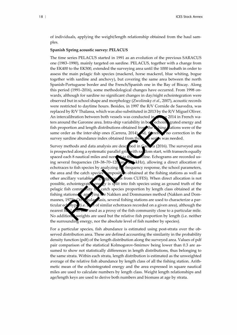
Survey methods and data analysis are described in Carrera (2016). The surveyed area is prospected along a systematic parallel grid with random start, with transects equally spaced each 8 nautical miles and normal to the shoreline. Echograms are recorded us-ing several frequencies (18–38–70–120 and 200 kHz), allowing a direct allocation of echotraces to fish species by analyzing the frequency response, the school parameters, the area and the catch species composition obtained at the fishing stations as well as other ancillary variables (e.g. egg counts from CUFES). When direct allocation is not possible, echointegrated energy is split into fish species using as ground truth of the pelagic fish community the catch species proportion by length class obtained at the fishing stations by applying the Nakken and Dommasnes method (Nakken and Dom-masnes, 1975). On regular basis, several fishing stations are used to characterize a par-ticular echotype (i.e. a set of similar echotraces recorded on a given area), although the nearest haul was also used as a proxy of the fish community close to a particular mile. No additional weights are used but the relative fish proportion by length (i.e. neither the surrounding energy, nor the absolute level of fish number by species).
For a particular species, fish abundance is estimated using post-strata over the ob-served distribution area. These are defined accounting the similarity in the probability density function (pdf) of the length distribution along the surveyed area. Values of pdf pair comparison of the statistical Kolmogorov-Smirnov being lower than 0.3 are as-sumed to show not statistically differences in length distributions, thus belonging to the same strata. Within each strata, length distribution is estimated as the unweighted average of the relative fish abundance by length class of all the fishing station. Arith-metic mean of the echointegrated energy and the area expressed in square nautical miles are used to calculate numbers by length class. Weight length relationships and age/length keys are used to derive both numbers and biomass at age by strata.
REPLACED
ICES Stock Annex | 19
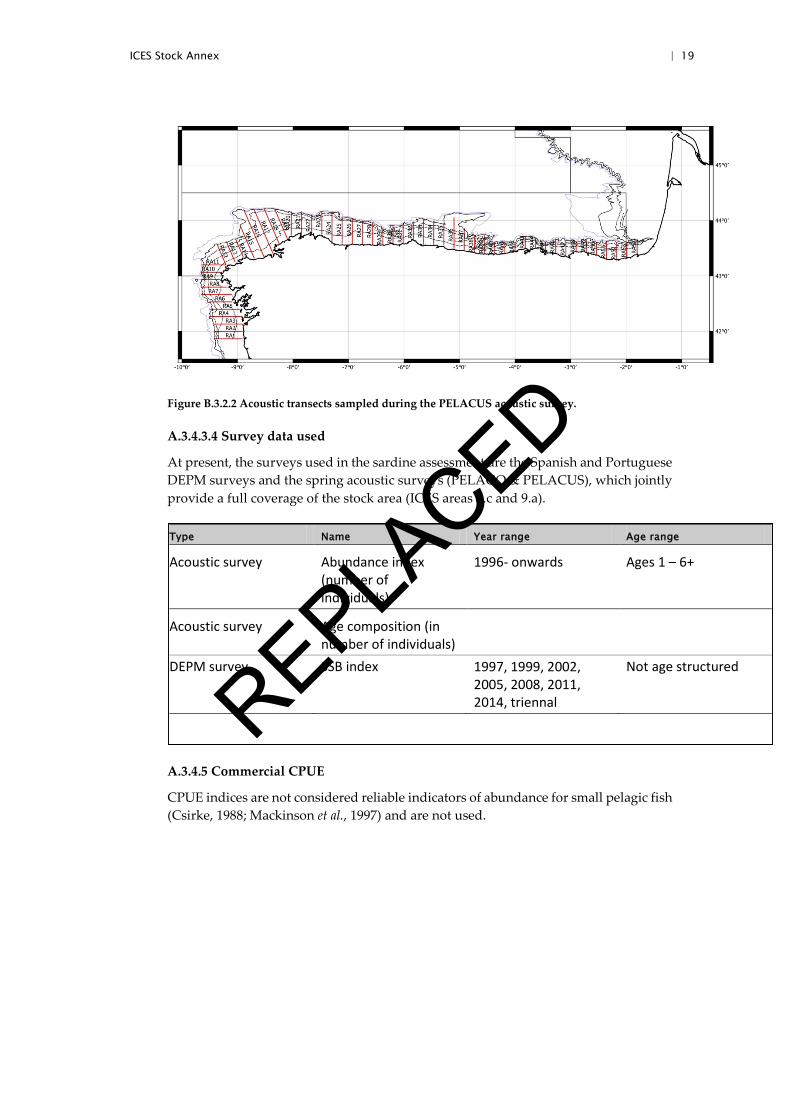
Figure B.3.2.2 Acoustic transects sampled during the PELACUS acoustic survey.
A.3.4.3.4 Survey data used
At present, the surveys used in the sardine assessment are the Spanish and Portuguese DEPM surveys and the spring acoustic surveys (PELAGO & PELACUS), which jointly provide a full coverage of the stock area (ICES areas 8.c and 9.a).
A.3.4.5 Commercial CPUE
CPUE indices are not considered reliable indicators of abundance for small pelagic fish (Csirke, 1988; Mackinson et al., 1997) and are not used.
Type Name Year range Age range
Acoustic survey Abundance index (number of individuals)
1996- onwards Ages 1 – 6+
Acoustic survey Age composition (in number of individuals)
DEPM survey SSB index 1997, 1999, 2002, 2005, 2008, 2011, 2014, triennal
Not age structured
REPLACED
20 | ICES Stock Annex
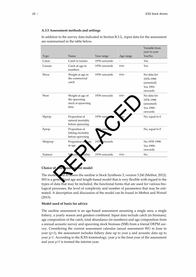
A.3.5 Assessment methods and settings
In addition to the survey data indicated in Section B.3.2., input data for the assessment are summarised in the table below.
Type Name Year range Age range
Variable from year to year Yes/No
Caton Catch in tonnes 1978–onwards - Yes
Canum Catch at age in numbers
1978–onwards 0-6+ Yes
Weca Weight at age in the commercial catch
1978–onwards 0-6+ No data for 1978–1990 (assumed) Yes 1991-onwards
West Weight at age of the spawning stock at spawning time
1978–onwards 0-6+ No data for 1978–1998 (assumed) Yes 1990–onwards
Mprop Proportion of natural mortality before spawning
1978–onwards 0-6+ No, equal to 0
Fprop Proportion of fishing mortality before spawning
1978–onwards No, equal to 0
Matprop Proportion mature at age
1978–onwards No 1978–1998 Yes 1999–onwards
Natmor Natural mortality 1978–onwards 0-6+ No
Choice of stock assessment model
The model used to assess the sardine is Stock Synthesis 3, version 3.24f (Methot, 2012). SS3 is a generalized age and length-based model that is very flexible with regard to the types of data that may be included, the functional forms that are used for various bio-logical processes, the level of complexity and number of parameters that may be esti-mated. A description and discussion of the model can be found in Methot and Wetzel (2013).
Model used of basis for advice
The sardine assessment is an age-based assessment assuming a single area, a single fishery, a yearly season and genders combined. Input data include catch (in biomass), age composition of the catch, total abundance (in numbers) and age composition from a annual acoustic survey and spawning stock biomass (SSB) from a trienal DEPM sur-vey. Considering the current assessment calendar (anual assessment WG in June in year (y+1), the assessment includes fishery data up to year y and acoustic data up to year y+1. According to the ICES terminology, year y is the final year of the assessment and year y+1 is termed the interim year.
REPLACED
ICES Stock Annex | 21
Assessment model configuration
The main model options are described below. A copy of the control file (sardine.ctl) including all model options is appended to the bottom of this Stock Annex.
Natural mortality are age specific input values as listed in Section B.2.2.
Growth is not modelled explicitly. Weights-at-age and maturity-at-age in the begin-ning of the year are input values calculated using DEPM survey data (Section B.2.1 and B.2.4).
Annual recruitments are parameters, defined as lognormal deviations from a Beverton-Holt stock recruitment model with steepness fixed at 0.71, the median steepness for Clupeidae from the meta-analysis by Myers et al. (1999). The input standard deviation of log number of recruits was set to 0.70 to be consistent with the residual mean stand-ard error of the recruitments estimated by the model.
Fishing mortality is applied as the hybrid method. This method does a Pope’s approx-imation to provide initial values for iterative adjustment of the continuous F values to closely approximate the observed catch.
Total catch biomass by year is assumed to be accurate and precise. The F values are tuned to match this catch.
Both the acoustic survey and the DEPM survey are assumed to be relative indices of abundance. The corresponding catchability coefficients are considered to be mean un-biased.
In the acoustic surveys, selectivity is assumed to be 1 at all ages (1 to 6+).
In the fishery, age selectivity is such that the parameter for each age is estimated as a random walk from the previous age. However, this applies only to ages 1, 2, 3 and 6+ in the fishery. Selectivity at ages 3 to 5 years in the fishery are bound, meaning that parameters for ages 4 and 5 are not estimated but assumed to be equal to the parameter estimated for age 3. Selectivity-at-age 0 is not estimated and is used as the reference age against which subsequent changes occur. The initial values for the fishery survey selectivity mimic dome-shaped patterns with a decline at the 6+ group. However, the range of initial values is wide and almost any pattern can be estimated.
The fishery selectivity is allowed to vary over time in the assessment period. Three periods are considered: 1978–1987, 1988–2005 and 2006–2016. Selectivity-at-age is esti-mated for each period and assumed to be fixed over time. The transition between pe-riods is done as a random walk.
The model estimates population biomass in the beginning of the last assessment year (interim year). There is data from the acoustic survey but not from the fishery (catch and age composition) for the interim year. Data used for the interim year are the fol-lowing: stock weights-at-age, catch biomass and catch weights-at-age are equal to those assumed for short term predictions (Section D). The fishery age composition in the in-terim year is assumed to be equal to that in the previous year. The fishery age compo-sition is included in the calculation of expected values but excluded from the objective function. Recruitment in the interim year is derived from the stock-recruitment rela-tionship.
The objective function is a log likelihood combining components for:
• Catch biomass (lognormal)
REPLACED
22 | ICES Stock Annex
• acoustic survey abundance index (lognormal) • DEPM survey SSB (lognormal) • fishery age composition (multinomial) • survey age composition (multinomial) • recruitment deviations (lognormal) • selectivity parameters (normal) • initial equilibrium catch (normal)
Estimates of data precision are included in the likelihood components for the abun-dance indices and age composition data as follows:
A standard error of 0.25 is assumed for all years both for the acoustic index (total num-ber of fish) and the DEPM index (SSB). In the likelihood components of each survey, annual log residuals are divided by the corresponding standard errors. Therefore, the two surveys and the years within each survey have equivalent weight in the objective function. The assumed standard error corresponds to a CV of 25% which is consistent with the average level of CVs estimated for the acoustic survey by geostatistics (range 12–43%, mean=23%, Marques, WD WKPELA2012) and Generalized Additive Models (Zwolinski et al., 2009) and with CVs estimated for the DEPM survey (range 14–30%, mean =22%, Angélico et al. WD1 WKPELA2017).
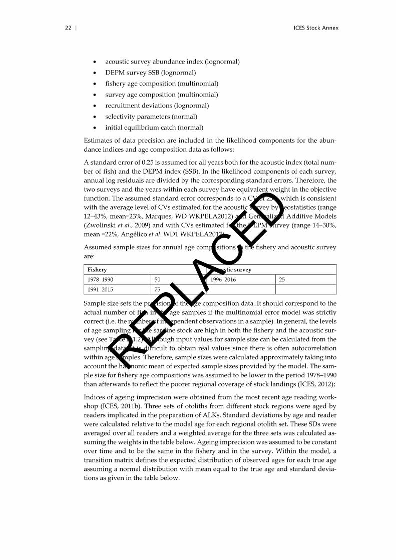
Assumed sample sizes for annual age compositions in the fishery and acoustic survey are:
Fishery Acoustic survey
1978–1990 50 1996–2016 25
1991–2015 75
Sample size sets the precision of the age composition data. It should correspond to the actual number of fish in the age samples if the multinomial error model was strictly correct (i.e. the number of independent observations in a sample). In general, the levels of age sampling for the sardine stock are high in both the fishery and the acoustic sur-vey (see Table B.1.2). Although input values for sample size can be calculated from the sampling data, it is difficult to obtain real values since there is often autocorrelation within age samples. Therefore, sample sizes were calculated approximately taking into account the harmonic mean of expected sample sizes provided by the model. The sam-ple size for fishery age compositions was assumed to be lower in the period 1978–1990 than afterwards to reflect the poorer regional coverage of stock landings (ICES, 2012);
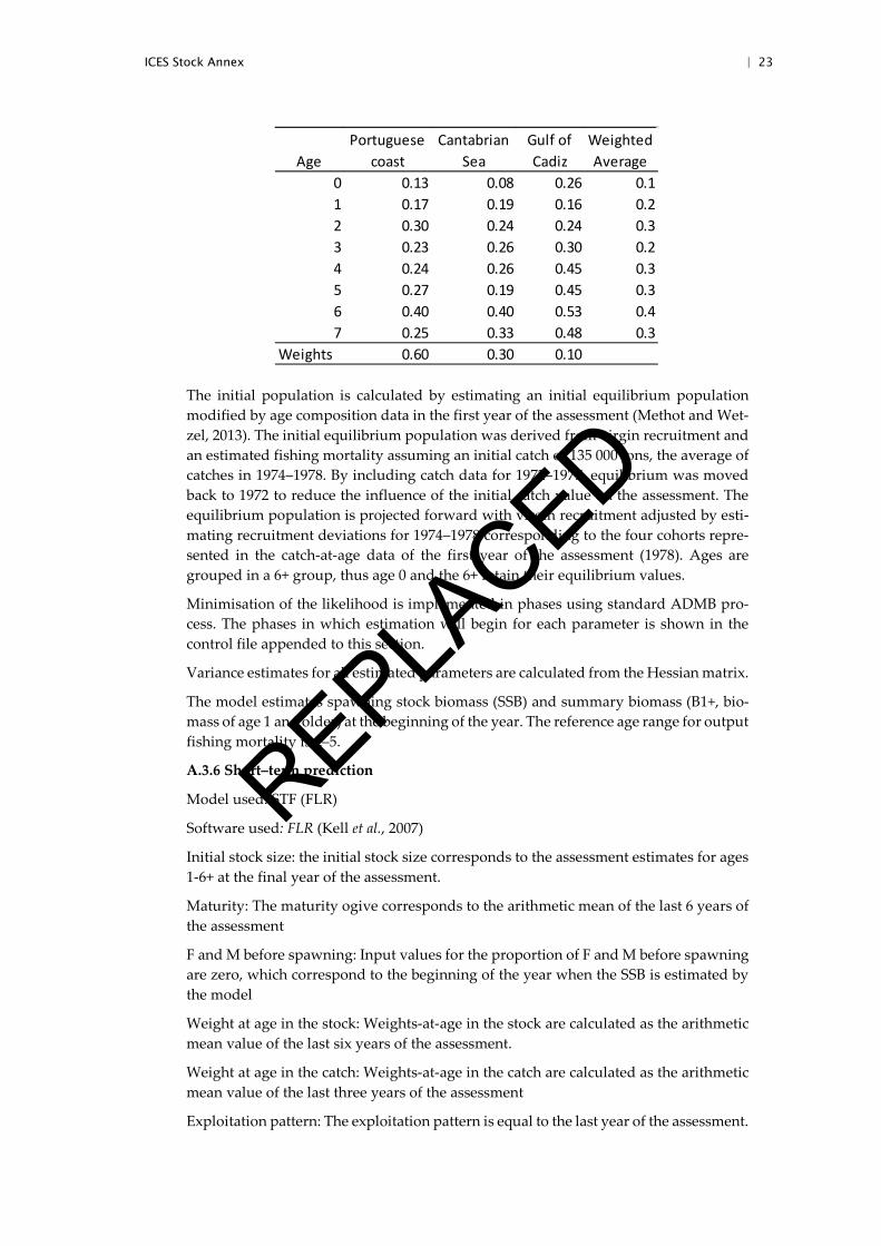
Indices of ageing imprecision were obtained from the most recent age reading work-shop (ICES, 2011b). Three sets of otoliths from different stock regions were aged by readers implicated in the preparation of ALKs. Standard deviations by age and reader were calculated relative to the modal age for each regional otolith set. These SDs were averaged over all readers and a weighted average for the three sets was calculated as-suming the weights in the table below. Ageing imprecision was assumed to be constant over time and to be the same in the fishery and in the survey. Within the model, a transition matrix defines the expected distribution of observed ages for each true age assuming a normal distribution with mean equal to the true age and standard devia-tions as given in the table below.
REPLACED
ICES Stock Annex | 23
The initial population is calculated by estimating an initial equilibrium population modified by age composition data in the first year of the assessment (Methot and Wet-zel, 2013). The initial equilibrium population was derived from virgin recruitment and an estimated fishing mortality assuming an initial catch of 135 000 tons, the average of catches in 1974–1978. By including catch data for 1972–1977, equilibrium was moved back to 1972 to reduce the influence of the initial catch value on the assessment. The equilibrium population is projected forward with virgin recruitment adjusted by esti-mating recruitment deviations for 1974–1978 corresponding to the four cohorts repre-sented in the catch-at-age data of the first year of the assessment (1978). Ages are grouped in a 6+ group, thus age 0 and the 6+ retain their equilibrium values.
Minimisation of the likelihood is implemented in phases using standard ADMB pro-cess. The phases in which estimation will begin for each parameter is shown in the control file appended to this section.
Variance estimates for all estimated parameters are calculated from the Hessian matrix.
The model estimates spawning stock biomass (SSB) and summary biomass (B1+, bio-mass of age 1 and older) at the beginning of the year. The reference age range for output fishing mortality is 2–5.
A.3.6 Short–term prediction
Model used: STF (FLR)
Software used: FLR (Kell et al., 2007)
Initial stock size: the initial stock size corresponds to the assessment estimates for ages 1-6+ at the final year of the assessment.
Maturity: The maturity ogive corresponds to the arithmetic mean of the last 6 years of the assessment
F and M before spawning: Input values for the proportion of F and M before spawning are zero, which correspond to the beginning of the year when the SSB is estimated by the model
Weight at age in the stock: Weights-at-age in the stock are calculated as the arithmetic mean value of the last six years of the assessment.
Weight at age in the catch: Weights-at-age in the catch are calculated as the arithmetic mean value of the last three years of the assessment
Exploitation pattern: The exploitation pattern is equal to the last year of the assessment.
AgePortuguese
coastCantabrian
SeaGulf of Cadiz
Weighted Average
0 0.13 0.08 0.26 0.11 0.17 0.19 0.16 0.22 0.30 0.24 0.24 0.33 0.23 0.26 0.30 0.24 0.24 0.26 0.45 0.35 0.27 0.19 0.45 0.36 0.40 0.40 0.53 0.47 0.25 0.33 0.48 0.3
Weights 0.60 0.30 0.10
REPLACED
24 | ICES Stock Annex
Intermediate year assumptions: Predictions are carried out with an Fmultiplier (usu-ally ranging from 0 to 2) assuming an Fsq equal to the average estimates of the last three years in the assessment or through a catch constraint based on regulations oper-ative in the interim year fishery.
Stock recruitment model used: Recruitment in the interim year and forecast year will be set equal to the geometric mean of the last five years
A.3.7 Medium-term prediction
Not carried out for this stock.
A.3.8 Long-term prediction
Not carried out for this stock.
A.3.9 Biological reference points
Currently, there are no defined reference points for the southern sardine stock and the basis of ICES advice is the Sardine Fishery Management Plan agreed by Spanish and Portuguese governments and evaluated by ICES to be provisionally precautionary (ICES, 2013a).
An estimation of biological reference points (BRP) for this stock was performed based on data from the latest assessment (ICES, 2017a). The methodology used followed the framework proposed in ICES (2017c) guidelines for fisheries management reference points. All statistical analyses were carried out in R environment (R core team 2015). Sardine’s latest stock information was converted to an ‘FLStock’ object using the ‘FLCore’ package (version 2.6.0.20170130). Simulations analyses were conducted with the package “msy” using the EqSim routines (https://github.com/ices-tools-prod/msy; ICES 2016c), a stochastic equilibrium reference point software that provides MSY ref-erence points based on the equilibrium distribution of stochastic projections.
Several scenarios were explored (whole time series with and without auto-correlation in recruitment; period 1993–2015 with Blim equal to the change point of the Hockey-stick S-R relationship and with Blim equal to B2000). Here we summarize the results for the base scenario (1993–2015 with Blim equal to the change point of the Hockey-stick S-R relationship), for further details on the other scenarios please see Wise et al. (WD to WKPELA2017 report in Annex 11+ ICES, 2017a).
In relation to stock productivity the group decided to use as the base scenario the pe-riod 1993–2015 similarly to the evaluation of the sardine MP (ICES, 2013a). There is evidence that sardine productivity has declined over time despite little or no unequiv-ocal evidence of a clear regime shift. In approximately the last 20 years, recruitment is at a lower level and biomass range is narrower than in the previous 15 years. Following the analysis performed in ICES (2013a) a productivity break was identified in 1992-1993 in the time series. The group agreed to maintain the same break as in the historical series and assume that the stock productivity in the period 1993–2015 is a plausible scenario for future stock dynamics. However, the group acknowledged that recruit-ments since 2006 are well below the average of the period 1993–2015 and recommends a close monitoring of the stock productivity and a re-evaluation of reference points in case there are signs that the current very low productivity continues in the future.
Simulations were performed with stochasticity in population biology parameters using the observed historical stock variation from the last six years (2010–2015). This period was chosen due to trends (positive) in stock and catches weight-at-age. Stock weight-at-age is calculated from DEPM surveys, which are carried out on a triennial basis. For
REPLACED
ICES Stock Annex | 25
years in between DEPM surveys, weight-at-age is linearly interpolated from adjacent surveys. A period of six years was chosen to include two survey estimates. This proce-dure is similar to the one adopted for the short term forecast (ICES, 2017a).
Several S–R relationships (Ricker, Beverton-Holt and Hockey-stick) were fit to the 1993-2015 data. The models showed comparable maximum likelihood estimates but the Hockey-stick achieved slightly better fits. The automatic weighting method imple-mented in EqSim (ICES, 2016c) was used to weight the combination of the three S-R models fitted from bootstrap samples of the SSB and recruit pairs. Again, the Hockey-stick had better results than the Ricker and Beverton-Holt with weights estimated to be 84%, 5% and 11%. The WG recognised the weighted S-R model had the advantage to acknowledge model uncertainty. However, the difference is small in this case as the Hockey-stick dominates the S–R combination by far (84% weight) and reference points from the two approaches were similar. The WG also considered that using a single S–R facilitates Management Strategy Evaluation (MSE) analyses in practical terms. In conclusion, the Hockey-stick S–R was adopted for the calculation of reference points.
Following ICES guidelines (ICES, 2017c), the S-R data of this stock is consistent with a Type 2 pattern given the wide dynamic range of SSB and evidence that recruitment is impaired. In this case, Blim is equal to the change point of a Hockey-stick model fitted to S–R data. The Blim candidate calculated as the change point of the Hockey-stick model was 337 448 tons. Bpa was derived as Bpa = Blim * exp(1 645 * σ), with σ = 0.17, the coefficient of variation of SSB2016 from the WKPELA 2017 assessment (ICES, 2017a).
Reference points were estimated based on the Hockey-stick S-R relationship with Blim and Bpa as defined above and no MSY Btrigger (i.e., without applying the ICES MSY AR). An initial simulation was performed over a range of F values (0–2) using historical variation in population and productivity parameters, re-sampled at random from the specified range of years but with no assessment/advice error.
The technical basis and the estimated BRP are shown in Table 2. Flim, the equilibrium F that gives a 50% probability of SSB>Blim was estimated at 0.25. Fpa was estimated as Fpa = Flim * exp(-1.645 * σ), with σ = 0.17, the coefficient of variation of apical F2015 from the WKPELA 2017 assessment. Fpa was estimated at 0.19. Follow-up simulations with the same settings as well as assessment/advice error in fishing mortality and in spawning stock biomass, estimated the median FMSY at 0.20.
Following ICES guidelines, and the fact that the stock has not been fished at/around FMSY for 5 years, MSY Btrigger = Bpa. With the ICES MSY AR (Advice Rule) and setting MSY Btrigger = Bpa the precautionary criterion for FMSY level was also tested, i.e. fishing at FMSY is precautionary in the sense that the probability of SSB falling below Blim in a year in long term simulations with fixed F is ≤ 5% (Fp.05). The Fp.05 was estimated at 0.12.
Fp.05 is well below FMSY. Although the reasons for this fact were not fully explored, a possible cause is that MSY Btrigger (= Bpa) is close to the mean stock biomass. It is also noted that Fp.05 estimates have a wide range with a highly right skewed distribution.
REPLACED
26 | ICES Stock Annex
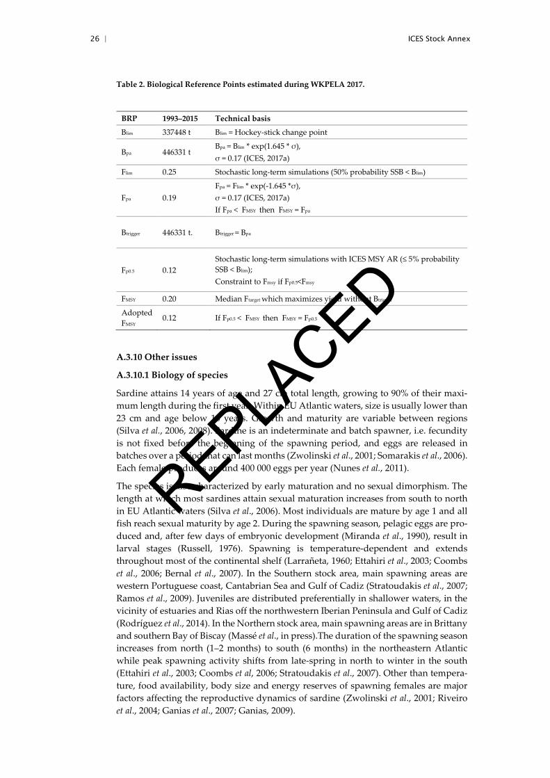
Table 2. Biological Reference Points estimated during WKPELA 2017.
BRP 1993–2015 Technical basis
Blim 337448 t Blim = Hockey-stick change point
Bpa 446331 t Bpa = Blim * exp(1.645 * σ), σ = 0.17 (ICES, 2017a)
Flim 0.25 Stochastic long-term simulations (50% probability SSB < Blim)
Fpa 0.19 Fpa = Flim * exp(-1.645 *σ), σ = 0.17 (ICES, 2017a) If Fpa < FMSY then FMSY = Fpa
Btrigger 446331 t. Btrigger = Bpa
Fp0.5 0.12 Stochastic long-term simulations with ICES MSY AR (≤ 5% probability SSB < Blim); Constraint to Fmsy if Fp0.5<Fmsy
FMSY 0.20 Median Ftarget which maximizes yield without Btrigger
Adopted FMSY
0.12 If Fp0.5 < FMSY then FMSY = Fp0.5
A.3.10 Other issues
A.3.10.1 Biology of species
Sardine attains 14 years of age and 27 cm total length, growing to 90% of their maxi-mum length during the first year. Within EU Atlantic waters, size is usually lower than 23 cm and age below 10 years. Growth and maturity are variable between regions (Silva et al., 2006, 2008). Sardine is an indeterminate and batch spawner, i.e. fecundity is not fixed before the beginning of the spawning period, and eggs are released in batches over a period that can last months (Zwolinski et al., 2001; Somarakis et al., 2006). Each female produces around 400 000 eggs per year (Nunes et al., 2011).
The species is also characterized by early maturation and no sexual dimorphism. The length at which most sardines attain sexual maturation increases from south to north in EU Atlantic waters (Silva et al., 2006). Most individuals are mature by age 1 and all fish reach sexual maturity by age 2. During the spawning season, pelagic eggs are pro-duced and, after few days of embryonic development (Miranda et al., 1990), result in larval stages (Russell, 1976). Spawning is temperature-dependent and extends throughout most of the continental shelf (Larrañeta, 1960; Ettahiri et al., 2003; Coombs et al., 2006; Bernal et al., 2007). In the Southern stock area, main spawning areas are western Portuguese coast, Cantabrian Sea and Gulf of Cadiz (Stratoudakis et al., 2007; Ramos et al., 2009). Juveniles are distributed preferentially in shallower waters, in the vicinity of estuaries and Rias off the northwestern Iberian Peninsula and Gulf of Cadiz (Rodríguez et al., 2014). In the Northern stock area, main spawning areas are in Brittany and southern Bay of Biscay (Massé et al., in press).The duration of the spawning season increases from north (1–2 months) to south (6 months) in the northeastern Atlantic while peak spawning activity shifts from late-spring in north to winter in the south (Ettahiri et al., 2003; Coombs et al, 2006; Stratoudakis et al., 2007). Other than tempera-ture, food availability, body size and energy reserves of spawning females are major factors affecting the reproductive dynamics of sardine (Zwolinski et al., 2001; Riveiro et al., 2004; Ganias et al., 2007; Ganias, 2009).
REPLACED
ICES Stock Annex | 27
A.3.10.2 Overview of stock assessments
From 2003 to 2012, the sardine stock was assessed using the age structured model AMCI (Assessment Model Combining Information from various sources, Skagen 2005). The year range and type of fishery data were the same as used at present. Up to 2006, the assessment was based on three independent acoustic surveys, the Spanish and Portuguese spring acoustic surveys and the Portuguese autumn acoustic survey and on the two national DEPM (Daily Egg Production Method) surveys. From 2006 to 2012 the Spanish and Portuguese surveys were combined to get indices of abundance covering the whole stock, both for the spring acoustic surveys and the DEPM surveys.
Because AMCI was not going to be maintained in the future, alternative models were explored in the 2012 benchmark (ICES, 2012). Stock Synthesis (SS3) was selected for the assessment in 2012 since it offered the same level of flexibility of AMCI and additional features, such as the possibility to incorporate uncertainty of input data in the variance of final estimates. The SS3 assessments carried out since the 2012 benchmark used the same (updated) data sets and similar model settings and assumptions as previously. In the WKPELA2017 adopted modelling of the sardine population with SS3 several data input have been revised and model settings updated as detailed in the sections above (and in the WKPELA2017 report).
A.3.10.3 Management and advice
There is no international TAC.
In order to ensure recovery of the sardine stock, Portugal and Spain developed a mul-tiannual management plan (ICES, 2013a). ICES concluded that the plan is provisionally precautionary (ICES, 2013b) and since 2015 advises were based on this MP.
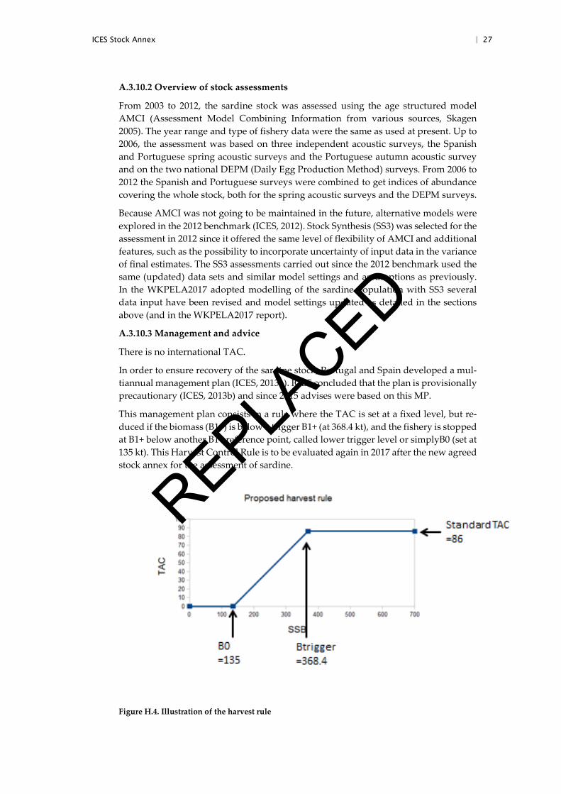
This management plan consists in a rule where the TAC is set at a fixed level, but re-duced if the biomass (B1+) is below a trigger B1+ (at 368.4 kt), and the fishery is stopped at B1+ below another B1+ reference point, called lower trigger level or simplyB0 (set at 135 kt). This Harvest Control Rule is to be evaluated again in 2017 after the new agreed stock annex for the assessment of sardine.
Figure H.4. Illustration of the harvest rule
REPLACED
28 | ICES Stock Annex
A.3.11 References
Abad E., Castro J., Punzón A., Abaunza P., 2008, Métiers of the Northern Spanish coastal fleet using purse seine gears. WD presented to the ICES WGWIDE 2008 meeting.
Alheit J., Licandro P., Coombs S., García A., Giráldez A., Garcia Santamaría M.T., Slotte A.,Tsi-kliras A.C., 2014, Atlantic Multidecadal Oscillation (AMO) modulates dynamics of small pelagic fishes and ecosystem regime shifts in the eastern North and Central Atlantic Journal of Marine Systems, 133:88–102.
Anon., 2006, Sardine dynamics and stock structure in the North-eastern Atlantic. Final Report. DGXIV Fisheries, European Commission, Brussel. Q5RS/2002/000818-available from [email protected].
Bernal M., Stratoudakis Y., Coombs S., Angelico M., Lago de Lanzós A., Porteiro C., Sagarminaga Y., Santos M., Uriarte A., Cunha E., Valdés L., Borchers D., 2007, Sardine spawning off the European Atlantic coast: characterization of spatio-temporal variability in spawning habi-tat. Progress in Oceanography, 74:210–227
Binet D., Samb B., Sidi M.T., Levenez J.J., Servain J., 1998, Sardine and other pelagic fisheries associated with multi-year trade wind increases, 212–233 pp. Paris: ORSTOM
Bode A., Carrera P., Lens S., 2003, The pelagic food web in the upwelling ecosystem of Galicia (NW Spain) during spring: natural abundance of stable carbon and nitrogen isotopes. ICES Journal of Marine Science, 60 (1): 11–22.
Bode A., Alvarez-Ossorio M.T., Carrera P., Lorenzo J., 2004, Reconstruction of trophic pathways between plankton and the North Iberian sardine (Sardina pilchardus) using stable isotopes. Scientia Marina, 68(1), 165–178.
Carrera P., 2014, INTERPELACUS 0414 Cruise report. 43 pp., Mimeo
Carrera P., 2016, PELACUS 0316 cruise report, 53 pp., Mimeo
Carrera P., Porteiro C., 2003, Stock dynamic of the Iberian sardine (Sardina pilchardus, W.) and its implication on the fishery off Galicia (NW Spain), Scientia Marina, 67 (1):245–258
Chouvelon T., Chappuis A., Bustamante P., Lefebvre S., Mornet F., Guillou G., Violamer L., Dupuy C., 2014, Trophic ecology of European sardine Sardina pilchardus and European an-chovy Engraulis encrasicolus in the Bay of Biscay (north-east Atlantic) inferred from δ 13 C and δ 15 N values of fish and identified mesozooplanktonic organisms. Journal of Sea Re-search, 85, 277–291.
Coombs S.H., Smyth T.J., Conway D.V.P., Halliday N.C., Bernal M., Stratoudakis Y., Alvarez P., 2006, Spawning season and temperature relationships for sardine (Sardina pilchardus) in the eastern North Atlantic. Journal of the Marine Biological Association of the United Kingdom, 86(05): 1245–1252.
Corten A., van de Kamp G.D., 1996, Variation in the abundance of southern fish species in the southern North Sea in relation to hydrography and wind. ICES J Mar Sci 53:1113–1119.
Costalago D., Navarro J., Álvarez-Calleja I., Palomera I., 2012, Ontogenetic and seasonal changes in the feeding habits and trophic levels of two small pelagic fish species. Marine Ecology Progress Series, 460: 169–181.
Costalago D., Palomera I., 2014, Feeding of European pilchard (Sardina pilchardus) in the north-western Mediterranean: from late larvae to adults. Scientia Marina, 78(1): 41–54.
Crawford R.J., Dyer B.M., 1995, Responses by four seabird species to a fluctuating availability of Cape anchovy Engraulis capensis off South Africa. Ibis, 137(3): 329–339.
Csirke J., 1988, Small shoaling pelagic fish stocks. In: Fish population dynamics, J.A. Gulland (Ed.), John Wiley y Sons., New York, 271–302.
REPLACED
ICES Stock Annex | 29
Cury P., Bakun, Crawford R.J., Jarre A., Quiñones R.A., Shannon L.J., Verheye H.M., 2000, Small pelagics in upwelling systems: patterns of interaction and structural changes in “wasp-waist” ecosystems. ICES Journal of Marine Science: Journal du Conseil, 57(3), 603–618.
Daunt F., Wanless S., Greenstreet S.P., Jensen H., Hamer K.C., Harris M.P., 2008, The impact of the sandeel fishery closure on seabird food consumption, distribution, and productivity in the north-western North Sea. Canadian Journal of Fisheries and Aquatic Sciences, 65(3): 362–381.
Ettahiri O., Berraho A., Vidy G., Ramdani M., 2003, Observation on the spawning of Sardina and Sardinella off the south Moroccan Atlantic coast (21–26 N). Fisheries Research, 60(2): 207–222.
Feijó, D., 2013, Caraterização da pesca do cerco na costa Portuguesa (Master Thesis). Faculdade de Ciências da Universidade do Porto, Porto, 91 pp.
Fernandes A.C., Feijó D., 2016, Analysis of sardine catches from onboard sampling in Portuguese purse seine fleet. Working Document for the ICES WGHANSA, Lorient, France, 24–29 June 2016.
Furness R.W., Edwards A.E., Oro D., 2007, Influence of management practices and of scavenging seabirds on availability of fisheries discards to benthic scavengers. Marine Ecology-Progress Series, 350: 235–244.
Ganias K., 2009, Linking sardine spawning dynamics to environmental variability. Estuarine, Coastal and Shelf Science, 84(3), 402–408.
Ganias K., Somarakis S., Koutsikopoulos C., Machias A., 2007, Factors affecting the spawning period of sardine in two highly oligotrophic Seas. Marine Biology, 151(4):1559–1569.
García-García L.M., Ruiz-Villarreal M., Bernal M., 2016, A biophysical model for simulating early life stages of sardine in the Iberian Atlantic stock. Fish. Res., 173 pp., 250–272.
Garrido S., Marçalo A., Zwolinski J., Van der Lingen C.D., 2007, Laboratory investigations on the effect of prey size and concentration on the feeding behaviour of Sardina pilchardus. Marine Ecology Progress Series, 330: 189–199.
Garrido S., Silva A., Pastor J., Dominguez R., Silva A.V., Santos A.M., 2015, Trophic ecology of pelagic fish species off the Iberian coast: diet overlap, cannibalism and intraguild predation. Mar Ecol Progr Ser 539: 271–285.
Guisande C., Cabanas J.M., Vergara A.R., Riveiro I., 2001, Effect of climate on recruitment success of Atlantic Iberian sardine Sardina pilchardus. Marine Ecology Progress Series. 223: 243–250.
ICES 2007, Report of the Working Group on the Assessment of Mackerel, Horse Mackerel, Sar-dine and Anchovy. ICES CM 2007/ACFM: 31.
ICES 2012, Report of the Benchmark Workshop on Pelagic Stocks (WKPELA 2012), 13–17 Febru-ary 2012, Copenhagen, Denmark. ICES CM 2012/ACOM:47, 572 pp.
ICES 2013a, Report of the Workshop to Evaluate the Management Plan for Iberian Sardine (WKSardineMP), 4–7 June 2013, Lisbon, Portugal. ICES CM 2013/ACOM:62, 82 pp.
ICES 2013b, Management plan evaluation for sardine in Divisions 8.c and 9.a. In Report of the ICES Advisory Committee, 2013. ICES Advice, 2013. Book 7, Section 7.3.5.1.
ICES 2015, Second Interim report of the Working Group on Acoustic and Egg Surveys for sardine and Anchovy in ICES Areas VII, VIII and IX (WGACEGG). 16–20 November 2015 Lowestoft, UK. Steering Group on Integrated Ecosystem Observation and Monitoring, ICES CM 2015/SSGIEOM:31, Ref ACOM and SCICOM, 396 pp.
ICES 2016a, Report of the Workshop on Atlantic Sardine (WKSAR), 26–30 September 2016, Lis-bon, Portugal. ICES CM 2016/ACOM:41, 351 pp.
ICES 2016b, Working Group on Southern Horse Mackerel, Anchovy and Sardine (WGHANSA), 24–29 June 2016, Lorient, France. ICES CM 2016/ACOM:17, 561 pp.
REPLACED
30 | ICES Stock Annex
ICES. 2016c. Report of the Workshop to consider FMSY ranges for stocks in ICES categories 1 and 2 in Western Waters (WKMSYREF4), 13–16 October 2015, Brest, France. ICES CM 2015/ACOM:58. 187 pp.
ICES 2017a, Report of the Benchmark Workshop on Pelagic Stocks (WKPELA 2017), 6–10 Febru-ary 2017, Lisbon, Portugal. ICES CM 2017/ACOM:35 in press.
ICES 2017b, Pelagic Surveys series for sardine and anchovy in ICES Areas VIII and IX (WGACEGG)-Towards an ecosystem approach. ICES Cooperative Research Report. Editors Massé, J., Uriarte. A., Angelico, M. M., and Carrera. (In press).
ICES, 2017c. ICES fisheries management reference points for category 1 and 2 stocks. In ICES Advice Technical Guidelines, 2017. ICES Advice 2017, Book 12, Section 12.4.3.1.
Jahncke J., Checkley D.M., Hunt G.L., 2004, Trends in carbon flux to seabirds in the Peruvian upwelling system: effects of wind and fisheries on population regulation. Fisheries Ocean-ography, 13 (3): 208–223.
Jemaa S., Dussene M., Cuvilier P., Bacha M., Khalaf G., Amara R, 2015, Comparaison du regime alimentaire de l’anchois (Engraulis encrasicolus) et de la sardine (Sardina pilchardus) en Atlan-tique et en Méditerranée. Lebanese Science Journal, 16: 7–22.
Kell, L. T., Mosqueira, I., Grosjean, P., Fromentin, J-M., Garcia, D., Hillary, R., Jardim, E., Mardle, S., Pastoors, M. A., Poos, J. J., Scott, F., Scott, R. D., 2007. FLR: an open-source framework for the evaluation and development of management strategies. ICES Journal of Marine Science, 64.
Kasapidis P., 2014, Chapter 2. Phylogeography and population genetics. In: Ganias K. (Ed.), Bi-ology and Ecology of Sardines and Anchovies, CRC Press, 375 pp., February 2014.
Larrañeta M.G., 1960, Synopsis of biological data on Sardina pilchardus of the Mediterranean and adjacent seas. Fisheries Division, Biology Branch, Food and Agriculture Organization of the United Nations.
Leitão F., Alms V., Erzini K., 2014, A multi-model approach to evaluate the role of environmental variability and fishing pressure in sardine fisheries. Journal of Marine Systems, 139, 128–138.
Lluch-Belda D, Lluch-Cota DB, Hernández-Vázquez, Salinas-Zavala CA (1992) Sardine popula-tion expansion in eastern boundary systems of the Pacific Ocean as related to sea surface temperature. South African Journal of Marine Science, 12(1): 147–155.
Mackinson S., Vasconcellos M. C., Pitcher, T. and Walters, C. J, 1997, Ecosystem impacts of har-vesting small pelagic fish in upwelling systems using a dynamic mass-balance model. Pro-ceedings Forage Fishes in Marine Ecosystems. Fairbanks: Anchorage, Alaska. Alaska Sea Grant College Program. AK9701: 15–30.
Magnussen E., 2011, Food and feeding habits of cod (Gadus morhua) on the Faroe Bank. ICES Journal of Marine Science, 68(9):1909–1917.
Massé J., Uriarte A., Angelico M.M., Carrera P., (in press). Pelagic surveys series for sardine and anchovy in ICES areas VIII and IX (WGACEGG)-Towards an ecosystem approach. ICES Cooperative Research Report.
Marçalo, A. 2009. Sardine (Sardina pilchardus) delayed mortality associated with purse-seine slip-ping: contributing stressors and responses. PhD Thesis, Faculdade de Ciências e Tecnologia. Universidade do Algarve, pp. 189.
Mesquita, C., 2008., Application of Linear Mixed Models in the study of LPUE patterns in the Portuguese purse seine fishery for sardine (Sardina pilchardus Walbaum, 1792). PhD Thesis. School of Biological Sciences, University of Aberdeen
Methot, R. M., 2012, User Manual for Stock Synthesis. Seattle, WA: NOAA Fisheries.
REPLACED
ICES Stock Annex | 31
Methot R.D., Wetzel C.R., 2013, Stock synthesis: a biological and statistical framework for fish stock assessment and fishery management. Fisheries Research, 142:86–99.
Meynier L., 2004, Food and feeding ecology of the common dolphin, Delphinus delphis, in the Bay of Biscay: Intraspecific dietary variation and food transfer modelling. Master thesis, Univer-sity of Aberdeen, Aberdeen, United Kingdom, 63 pp.
Miranda A., Cal R.M., Iglesias J., 1990, Effect of temperature on the development of eggs and larvae of sardine Sardina pilchardus Walbaum in captivity. Journal of Experimental Marine Biology and Ecology 140 (1): 69–77.
Myers, R.A., Bowen, K.G., and Barrowman, N.J, 1999, The maximum reproductive rate of fish at low population sizes. Canadian Journal of Fisheries and Aquatic Sciences, 56:2404–2419.
Nakken, O. and Dommasnes A., 1975, The application for an echo integration system in investi-gations on the stock strength of the Barents Sea capelin (Mallotus villosus, Müller) 1971–74. ICES CM 1975/B:25.
Nunes C, Silva A, Marques V, Ganias K. 2011. Integrating fish size, condition, and population demography in the estimation of sardine annual fecundity. Ciencias Marinas, 37, 564–584
Parrish R.H., Serra R., Grant W.S., 1989, The monotypic sardines, Sardina and Sardinops: their taxonomy, stock structure, and zoogeography. Can. J. Fish. Aquat. Sci. 46: 2019–2036.
R Core Team. 2015. R: A language and environment for statistical computing. R Foundation for Statistical Computing, Vienna, Austria. URL http://www.R-project.org/.
Ramos S., Ré P., Bordalo A.A., 2009, New insights into the early life ecology of Sardina pilchardus (Walbaum, 1792) in the northern Iberian Atlantic. Scientia Marina 73 (3):449–49.
Rice J., 1995, Food web theory, marine food webs and what climate changes may do to northern marine fish populations. In: Beamish R.J. (Ed), Climate Change and Northern Fish Popula-tions. Canadian Special Publication Fisheries & Aquatic Science, 121:561–568.
Riveiro I., Guisande C., Maneiro I., Vergara A.R., 2004, Parental effects in the European sardine Sardina pilchardus. Marine Ecology Progress Series, 274, 225–234.
Rodríguez S., Marques V., Angélico M.M., Silva A., 2014, Identifying essential juvenile habitat for sardine (Sardina pilchardus (Walbaum, 1972)) along the Portuguese coast and Gulf of Cá-diz. Poster presented at the Johan Hjort Symposium on Recruitment Dynamics and Stock Variability 7–9 November 2014 Bergen (Norway).
Russell F.S., 1976, The eggs and planktonic stages of British marine fishes. Academic Press, New York.
Stratoudakis Y., Coombs S., Lago de Lanzós A., Halliday N., Costas G., Caneco B., Franco C., Conway D., Santos M.B., Silva A., Bernal M., 2007, Sardine (Sardina pilchardus) spawnings-easonality in European waters of the northeast Atlantic. Marine Biology, 152(1): 201–212.
Santos A.M.P., Chícharo A., Dos Santos A., Miota T., Oliveira P.B., Peliz A., and Ré P., 2007 Phys-ical–biological interactions in the life history of small pelagic fish in the Western Iberia Upwelling Ecosystem. Progress in Oceanography, 74: 192–209.
Santos M.B, Pierce G.J., López A., Martínez J.A., Fernández M.T., Ieno E., Mente E., Porteiro C., Carrera P. and Meixide M., 2004, Variability in the diet of common dolphins (Delphinus del-phis) in Galician waters 1991–2003 and relationship with prey abundance. ICES CM 2004/Q:09
Santos M.B., González-Quirós R., Riveiro I., Cabanas J.M., Porteiro C., Pierce G.J., 2012, Cycles, trends, and residual variation in the Iberian sardine (Sardina pilchardus) recruitment series and their relationship with the environment. ICES Journal of Marine Science: Journal du Conseil, 69(5): 739–750.
Santos M.B, German I., Correia D., Read F.L., Martinez-Cedeira J., Caldas M., López A., Velasco F., Pierce G.J., 2013, Long-term variation in common dolphin diet in relation to prey abun-dance. Marine Ecology Progress Series 481, 249–268.
REPLACED
32 | ICES Stock Annex
Santos M.B., Saavedra C., Pierce G.J., 2014, Quantifying the predation on sardine and hake by cetaceans in the Atlantic waters of the Iberian Peninsula. Deep Sea Research II: Topical Stud-ies in Oceanography 106, 232–244.
Silva M.A., 2001, Diet of common dolphins, Delphinus delphis, off the Portuguese continental coast. Journal of the Marine Biological Association of the U.K. 87: 231–241.
Silva A., Santos M.B., Caneco B., Pestana G., Porteiro C., Carrera P., Stratoudakis Y., 2006, Tem-poral and geographic variability of sardine maturity at length in the north-eastern Atlantic and the western Mediterranean. ICES Journal of Marine Science: 63(4): 663–676.
Silva A., Carrera P., Masse J., Uriarte A., Santos M., Oliveira P., Soares E., Porteiro C., Stratou-dakis Y., 2008, Geographic variability of sardine growth across the north-eastern Atlantic and the Mediterranean Sea. Fisheries Research: 90 (1–3): 56–69.
Silva A., Moreno A., Rivero I., Santos B., Pita C., Garcia R., J., Villasante S., Pawlowski L., Duha-mel E., 2015, Sardine Fisheries: Resource assessment and social and economic situation. EU Parliament. European Parliament-Directorate-General for Internal Policies Directorate B-Structural and Cohesion Policy, Brussels, 55 pp.
Stratoudakis Y., Marçalo A., 2002, Sardine slipping during purse-seining off northern Portugal. ICES Journal of Marine Science 59:1256–1262
Thompson P.M., McConnell B.J., Tollit D.J., MacKay A., Hunter C., Racey P.A., 1996, Compara-tive distribution, movements and diet of harbour and grey seals from the Moray Firth, N.E. Scotland. Journal of Applied Ecology, 33:1572–1584.
Uriarte, A., Prouzet, P. and Villamor, B. 1996. Bay of Biscay and Ibero Atlantic anchovy popula-tions and their fisheries. Scientia Marina, 60 (Supl. 2): 237–255.
Varela M., Larrañaga A., Costas E., Rodriguez B., 1988, Contenido estomacal de la sardina (Sar-dina pilchardus Walbaum) durante la campaña Saracus 871 en las plataformas Cantábrica y de Galicia en febrero de 1971. Boletín Instituto Español de Oceanografía, 5: 17–28.
Villamor B., Abaunza P., Lucio P. and Porteiro C., 1997, Distribution and age structure of macke-rel (Scomber scombrus L.) and horse mackerel (Trachurus Trachurus L.) in the northern coast of Spain. Scientia Marina. 61: 345–366.
Walter J.F., Austin H.M., 2003, Diet composition of large striped bass (Morone saxatilis) in Ches-apeake Bay. Fishery Bulletin, 101:414–423
Weise M.J., Harvey J.T., 2008, Temporal variability in ocean climate and California sea lion diet and biomass consumption: implications for fisheries management. Marine Ecology Progress Series, 373: 157–172.
Zwolinski J., Stratoudakis Y., Sares E., 2001, Intra-annual variation in the batch fecundity of sar-dine off Portugal. Journal of Fish Biology, 58(6): 1633–1645.
Zwolinski J., Morais A., Marques V., Stratoudakis Y., and Fernandes, P., 2007, Diel variation in the vertical distribution and schooling behaviour of sardine (Sardina pilchardus) off Portugal. ICES Journal of Marine Science, 64: 963–972.
Zwolinski J., Fernandes P., Marques V., and Stratoudakis, Y., 2009, Estimating fish abundance from acoustic surveys: calculating variance due to acoustic backscatter and length distribu-tion error. Can. J. Fish. Aquat. Sci, 66:2081-2095.
REPLACED
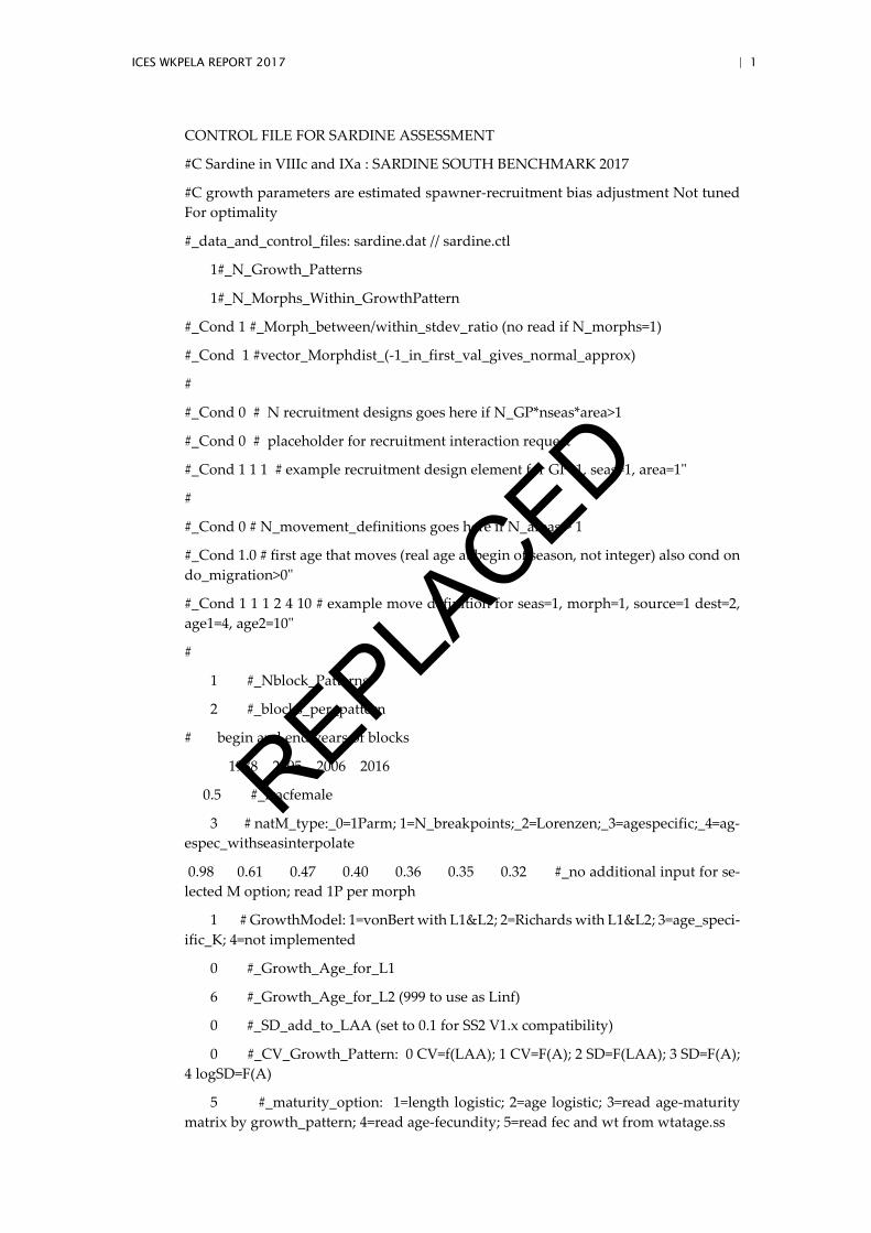
ICES WKPELA REPORT 2017 | 1
CONTROL FILE FOR SARDINE ASSESSMENT
#C Sardine in VIIIc and IXa : SARDINE SOUTH BENCHMARK 2017
#C growth parameters are estimated spawner-recruitment bias adjustment Not tuned For optimality
#_data_and_control_files: sardine.dat // sardine.ctl
1#_N_Growth_Patterns
1#_N_Morphs_Within_GrowthPattern
#_Cond 1 #_Morph_between/within_stdev_ratio (no read if N_morphs=1)
#_Cond 1 #vector_Morphdist_(-1_in_first_val_gives_normal_approx)
#
#_Cond 0 # N recruitment designs goes here if N_GP*nseas*area>1
#_Cond 0 # placeholder for recruitment interaction request
#_Cond 1 1 1 # example recruitment design element for GP=1, seas=1, area=1"
#
#_Cond 0 # N_movement_definitions goes here if N_areas > 1
#_Cond 1.0 # first age that moves (real age at begin of season, not integer) also cond on do_migration>0"
#_Cond 1 1 1 2 4 10 # example move definition for seas=1, morph=1, source=1 dest=2, age1=4, age2=10"
#
1 #_Nblock_Patterns
2 #_blocks_per_pattern
# begin and end years of blocks
1988 2005 2006 2016
0.5 #_fracfemale
3 # natM_type:_0=1Parm; 1=N_breakpoints;_2=Lorenzen;_3=agespecific;_4=ag-espec_withseasinterpolate
0.98 0.61 0.47 0.40 0.36 0.35 0.32 #_no additional input for se-lected M option; read 1P per morph
1 # GrowthModel: 1=vonBert with L1&L2; 2=Richards with L1&L2; 3=age_speci-ific_K; 4=not implemented
0 #_Growth_Age_for_L1
6 #_Growth_Age_for_L2 (999 to use as Linf)
0 #_SD_add_to_LAA (set to 0.1 for SS2 V1.x compatibility)
0 #_CV_Growth_Pattern: 0 CV=f(LAA); 1 CV=F(A); 2 SD=F(LAA); 3 SD=F(A); 4 logSD=F(A)
5 #_maturity_option: 1=length logistic; 2=age logistic; 3=read age-maturity matrix by growth_pattern; 4=read age-fecundity; 5=read fec and wt from wtatage.ss
REPLACED
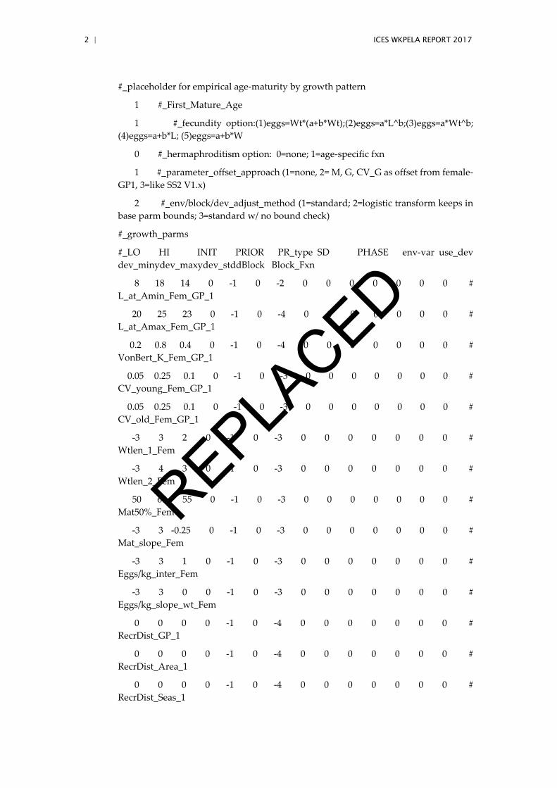
2 | ICES WKPELA REPORT 2017
#_placeholder for empirical age-maturity by growth pattern
1 #_First_Mature_Age
1 #_fecundity option:(1)eggs=Wt*(a+b*Wt);(2)eggs=a*L^b;(3)eggs=a*Wt^b; (4)eggs=a+b*L; (5)eggs=a+b*W
0 #_hermaphroditism option: 0=none; 1=age-specific fxn
1 #_parameter_offset_approach (1=none, 2= M, G, CV_G as offset from female-GP1, 3=like SS2 V1.x)
2 #_env/block/dev_adjust_method (1=standard; 2=logistic transform keeps in base parm bounds; 3=standard w/ no bound check)
#_growth_parms
#_LO HI INIT PRIOR PR_type SD PHASE env-var use_dev dev_minydev_maxydev_stddBlock Block_Fxn
8 18 14 0 -1 0 -2 0 0 0 0 0 0 0 # L_at_Amin_Fem_GP_1
20 25 23 0 -1 0 -4 0 0 0 0 0 0 0 # L_at_Amax_Fem_GP_1
0.2 0.8 0.4 0 -1 0 -4 0 0 0 0 0 0 0 # VonBert_K_Fem_GP_1
0.05 0.25 0.1 0 -1 0 -3 0 0 0 0 0 0 0 # CV_young_Fem_GP_1
0.05 0.25 0.1 0 -1 0 -3 0 0 0 0 0 0 0 # CV_old_Fem_GP_1
-3 3 2 0 -1 0 -3 0 0 0 0 0 0 0 # Wtlen_1_Fem
-3 4 3 0 -1 0 -3 0 0 0 0 0 0 0 # Wtlen_2_Fem
50 60 55 0 -1 0 -3 0 0 0 0 0 0 0 # Mat50%_Fem
-3 3 -0.25 0 -1 0 -3 0 0 0 0 0 0 0 # Mat_slope_Fem
-3 3 1 0 -1 0 -3 0 0 0 0 0 0 0 # Eggs/kg_inter_Fem
-3 3 0 0 -1 0 -3 0 0 0 0 0 0 0 # Eggs/kg_slope_wt_Fem
0 0 0 0 -1 0 -4 0 0 0 0 0 0 0 # RecrDist_GP_1
0 0 0 0 -1 0 -4 0 0 0 0 0 0 0 # RecrDist_Area_1
0 0 0 0 -1 0 -4 0 0 0 0 0 0 0 # RecrDist_Seas_1
REPLACED
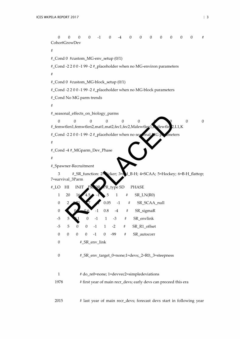
ICES WKPELA REPORT 2017 | 3
0 0 0 0 -1 0 -4 0 0 0 0 0 0 0 # CohortGrowDev
#
#_Cond 0 #custom_MG-env_setup (0/1)
#_Cond -2 2 0 0 -1 99 -2 #_placeholder when no MG-environ parameters
#
#_Cond 0 #custom_MG-block_setup (0/1)
#_Cond -2 2 0 0 -1 99 -2 #_placeholder when no MG-block parameters
#_Cond No MG parm trends
#
#_seasonal_effects_on_biology_parms
0 0 0 0 0 0 0 0 0 0 #_femwtlen1,femwtlen2,mat1,mat2,fec1,fec2,Malewtlen1,malewtlen2,L1,K
#_Cond -2 2 0 0 -1 99 -2 #_placeholder when no seasonal MG parameters
#
#_Cond -4 #_MGparm_Dev_Phase
#
#_Spawner-Recruitment
3 #_SR_function: 2=Ricker; 3=std_B-H; 4=SCAA; 5=Hockey; 6=B-H_flattop; 7=survival_3Parm
#_LO HI INIT PRIOR PR_type SD PHASE
1 20 16 4.5 -1 5 1 # SR_LN(R0)
0 2 0.71 0.7 -1 0.05 -1 # SR_SCAA_null
0 4 0.7 0.6 -1 0.8 -4 # SR_sigmaR
-5 5 0.1 0 -1 1 -3 # SR_envlink
-5 5 0 0 -1 1 -2 # SR_R1_offset
0 0 0 0 -1 0 -99 # SR_autocorr
0 #_SR_env_link
0 #_SR_env_target_0=none;1=devs;_2=R0;_3=steepness
1 # do_re0=none; 1=devvec2=simpledeviations
1978 # first year of main recr_devs; early devs can preceed this era
2015 # last year of main recr_devs; forecast devs start in following year
REPLACED
4 | ICES WKPELA REPORT 2017
2 #_recdev phase
1 # (0/1) to read 13 advanced options
-4 #_recdev_early_start (0=none; neg value makes relative to recdev_start)
2 #_recdev_early_phase
-1 #_forecast_recruitment phase (incl. late recr) (0 value resets to max-phase+1)
1 #_lambda for Fcast_recr_like occurring before endyr+1
1900 #_last_early_yr_nobias_adj_in_MPD
1900 #_first_yr_fullbias_adj_in_MPD
1900 #_last_yr_fullbias_adj_in_MPD
1900 #_first_recent_yr_nobias_adj_in_MPD
1 #_max_bias_adj_in_MPD (-1 to override ramp and set biasadj=1.0 for all estimated recdevs)
0 #_period of cycles in recruitment (N parms read below)
-5 #min rec_dev
5 #max rec_dev
0 #_read_recdevs
#_end of advanced SR options
#
#_placeholder for full parameter lines for recruitment cycles
# read specified recr devs
#_Yr Input_value
#
# all recruitment deviations
REPLACED
ICES WKPELA REPORT 2017 | 5
#DisplayOnly 0 # Main_InitAge_4
#DisplayOnly 0 # Main_RecrDev_1991
#DisplayOnly 0 # ForeRecr_2012
#
#Fishing Mortality info
0.3 # F ballpark for tuning early phases
-2001 # F ballpark year (neg value to disable)
3 # F_Method: 1=Pope; 2=instan. F; 3=hybrid (hybrid is recommended)
2 # max F or harvest rate, depends on F_Method
# no additional F input needed for Fmethod 1
# if Fmethod=2; read overall start F value; overall phase; N detailed inputs to read
# if Fmethod=3; read N iterations for tuning for Fmethod 3
4 # N iterations for tuning F in hybrid method (recommend 3 to 7)
#
#_initial_F_parms
#_LO HI INIT PRIOR PR_type SD PHASE
-1 2 0.3 0.3 -1 0.2 1 # InitF_1purse_seine
#
#_Q_setup
# Q_type options: <0=mirror, 0=median_float, 1=mean_float, 2=parameter, 3=parm_w_random_dev, 4=parm_w_randwalk, 5=mean_unbiased_float_as-sign_to_parm
#_for_env-var:_enter_index_of_the_env-var_to_be_linked
#_Den-deenv-var extra_seQ_type
0 0 0 0 # 1purse_seine
0 0 0 2 # 2Acoustic_survey
0 0 0 2 # 3DEPM_survey
#
#_Cond 0 #_If q has random component, then 0=read one parm for each fleet with ran-dom q; 1=read a parm for each year of index
#_Q_parms(if_any)
# LO HI INIT PRIOR PR_type SD PHASE
-3 3 0 0 -1 1 1 # Q_base_2_Acoustic survey
-3 3 0 0 -1 1 1 # Q_base_3_DEPM_survey
REPLACED
6 | ICES WKPELA REPORT 2017
#_size_selex_types
#_PatterDiscard Male Special
0 0 0 0 # 1purse_seine
0 0 0 0 # 2Acoustic_survey
30 0 0 0 # 3DEPM_survey
#_age_selex_types
#_Patter___ Male Special
17 0 0 0 # 1purse_seine
17 0 0 0 # 2Acoustic_survey
10 0 0 0 # 3DEPM_survey
#_LO HI INIT PRIOR PR_type SD PHASE env-var use_dev dev_minydev_maxydev_stddBlock Block_Fxn
-4 4 0 0 -1 0.01 -2 0 0 0 0 0 0 0 # AgeSel_1P_0_purse_seine
-3 3 0.9 0.5 -1 0.01 2 0 0 0 0 0 1 3 # AgeSel_1P_1_purse_seine
-4 4 0.4 0.5 -1 0.01 2 0 0 0 0 0 1 3 # AgeSel_1P_2_purse_seine
-4 4 0.1 0.3 -1 0.01 2 0 0 0 0 0 1 3 # AgeSel_1P_3_purse_seine
-4 4 0 0.1 -1 0.01 -2 0 0 0 0 0 0 0 # AgeSel_1P_4_purse_seine
-4 4 0 0.1 -1 0.01 -2 0 0 0 0 0 0 0 # AgeSel_1P_5_purse_seine
-4 4 -0.5 0.5 -1 0.01 2 0 0 0 0 0 1 3 # AgeSel_1P_6_purse_seine
-1000 -1000 -1000 -6 -1 0.01 -2 0 0 0 0 0 0 0 # AgeSel_2P_0_Acoustic_survey
-4 4 0 0.5 -1 0.01 -2 0 0 0 0 0 0 0 # AgeSel_2P_1_Acoustic_survey
-4 4 0 0 -1 0.01 -2 0 0 0 0 0 0 0 # AgeSel_2P_2_Acoustic_survey
-4 4 0 0 -1 0.01 -2 0 0 0 0 0 0 0 # AgeSel_2P_3_Acoustic_survey
-4 4 0 0 -1 0.01 -2 0 0 0 0 0 0 0 # AgeSel_2P_4_Acoustic_survey
-4 4 0 0 -1 0.01 -2 0 0 0 0 0 0 0 # AgeSel_2P_5_Acoustic_survey
-4 4 0 -1 -1 0.01 -2 0 0 0 0 0 0 0 # AgeSel_2P_6_Acoustic_survey
REPLACED
ICES WKPELA REPORT 2017 | 7
#_Cond 0 #_custom_sel-env_setup (0/1)
#_Cond -2 2 0 0 -1 99 -2 #_placeholder when no enviro fxns
1 #_custom_sel-blk_setup (0/1)
-4 4 0.9 1 -1 0.01 2 # AgeSel_1P_1_purse_seine_BLK1delta_1988
-4 4 0.9 1 -1 0.01 2 # AgeSel_1P_1_purse_seine_BLK1delta_2006
-4 4 0.4 1 -1 0.01 2 # AgeSel_1P_2_purse_seine_BLK1delta_1988
-4 4 0.4 1 -1 0.01 2 # AgeSel_1P_2_purse_seine_BLK1delta_2006
-4 4 0.1 1 -1 0.01 2 # AgeSel_1P_3_purse_seine_BLK1delta_1988
-4 4 0.1 1 -1 0.01 2 # AgeSel_1P_3_purse_seine_BLK1delta_2006
-4 4 -0.5 1 -1 0.01 2 # AgeSel_1P_6_purse_seine_BLK1delta_1988
-4 4 -0.5 1 -1 0.01 2 # AgeSel_1P_6_purse_seine_BLK1delta_2006
#_Cond -2 2 0 0 -1 99 -2 #_placeholder when no block usage
#_Cond No selex parm trends
#_Cond 4 # placeholder for selparm_Dev_Phase
1 #_Cond 1 #_env/block/dev_adjust_method (1=standard; 2=logistic trans to keep in base parm bounds; 3=standard w/ no bound check)
#
# Tag loss and Tag reporting parameters go next
0 # TG_custom: 0=no read; 1=read if tags exist
#_Cond -6 6 1 1 2 0.01 -4 0 0 0 0 0 0 0 #_placeholder if no parameters
#
1 #_Variance_adjustments_to_input_values
#_fleet: 1 2 3
0 0 0 #_add_to_survey_CV
0 0 0 #_add_to_discard_stddev
0 0 0 #_add_to_bodywt_CV
0 0 0 #_mult_by_lencomp_N
1 1 1 #_mult_by_agecomp_N
1 1 1 #_mult_by_size-at-age_N
#
REPLACED
8 | ICES WKPELA REPORT 2017
4 #_maxlambdaphase
1 #_sd_offset
#
3 # number of changes to make to default Lambdas (default value is 1.0)
# Like_comp codes: 1=surv; 2=disc; 3=mnwt; 4=length; 5=age; 6=SizeFreq; 7=sizeage; 8=catch;
# 9=init_equ_catch; 10=recrdev; 11=parm_prior; 12=parm_dev; 13=CrashPen; 14=Morphcomp; 15=Tag-comp; 16=Tag-negbin
#like_comp fleet/survey phase value sizefreq_method
9 1 1 1 1
4 2 2 1 1
4 2 3 1 1
# lambdas (for info only; columns are phases)
# 0 0 0 0 #_CPUE/survey:_1
# 1 1 1 1 #_CPUE/survey:_2
# 1 1 1 1 #_CPUE/survey:_3
# 1 1 1 1 #_agecomp:_1
# 1 1 1 1 #_agecomp:_2
# 0 0 0 0 #_agecomp:_3
# 1 1 1 1 #_init_equ_catch
# 1 1 1 1 #_recruitments
# 1 1 1 1 #_parameter-priors
# 1 1 1 1 #_parameter-dev-vectors
# 1 1 1 1 #_crashPenLambda
1 # (0/1) read specs for more stddev reporting
0 2 -1 7 0 7 -1 2016 6 # placeholder for selex type, len/age, year, N selex bins, Growth pattern, N growth ages, NatAge_area(-1 for all), NatAge_yr, N Natages
5 16 27 38 46 0 0 # vector with selex std bin picks (-1 in first bin to self-generate)
1 2 14 26 40 0 0 # vector with growth std bin picks (-1 in first bin to self-generate)
1 2 3 4 5 6 # vector with N-at-age std bin picks (-1 in first bin to self-generate)
999
REPLACED