Stochastic Survival Models with Competing Risks and Covariates

Stochastic Survival Models with Competing Risks and CovariatesAuthor(s): Gerald J. BeckSource: Biometrics, Vol. 35, No. 2 (Jun., 1979), pp. 427-438Published by: International Biometric SocietyStable URL: http://www.jstor.org/stable/2530345 .

Accessed: 28/06/2014 11:34

Your use of the JSTOR archive indicates your acceptance of the Terms & Conditions of Use, available at .http://www.jstor.org/page/info/about/policies/terms.jsp

.JSTOR is a not-for-profit service that helps scholars, researchers, and students discover, use, and build upon a wide range ofcontent in a trusted digital archive. We use information technology and tools to increase productivity and facilitate new formsof scholarship. For more information about JSTOR, please contact [email protected].

.

International Biometric Society is collaborating with JSTOR to digitize, preserve and extend access toBiometrics.

http://www.jstor.org

This content downloaded from 193.105.245.57 on Sat, 28 Jun 2014 11:34:12 AMAll use subject to JSTOR Terms and Conditions

http://www.jstor.org/action/showPublisher?publisherCode=ibs

http://www.jstor.org/stable/2530345?origin=JSTOR-pdf

http://www.jstor.org/page/info/about/policies/terms.jsp


BIOMETRICS 35, 427-438 June, 1979

Stochastic Survival Models with Competing Risks and Covariates GERALD J. BECK

Department of Epidemiology and Public Health (Biometry), Yale School of Medicine, New Haven, Connecticut 06510, U.S.A.

Summary

In survival analysis, information of covariates has been used to evaluate their importance 1Z1 predicting the survival probability oif a given individual. This paper develops a stochastic survival model which incorporates covar&tes and allows two states of "health" and several coss1peting risks of death. The transition intensity functions can have an exponential or Weibull form but depend upon the covariates. Other generalizations of the model are presented. The model of Lagakos (1976) is a special case of the models proposed here. The asymptotic theory of the maximum likelihood estimates and a goodness-of-fit procedure is diseussed along with tS1e estimation of the survival, transition and competing risks probabilities. These models are applicable to data collected in a clinical trial or prospective study and can distinguish between end-of- study and loss-to-follow-up censoring. An application is given which analyzes the survival of patients in a heart transplant program.

1. Introduction

Stochastic survival models which adjust for each individual's covariate information have been employed since first introduced by Feigl and Zelen (1965). More recently, models which allow more than the two states of alive and dead have been proposed (Beck 1975, and Lagakos 1976). Such models have application to the study of survival in prospective studies and clinical trials where study subjects are followed to determine their status or well-being over a period of time. During each individual's observation period, he may be classified into various stages of health and may die from one of several causes of death. For example, a prospective study may begin with healthy persons who are followed to determine which of them develop a specific disease, such as coronary heart disease, how it affects their survival, and which covariables (e.g., age, blood pressure, smoking history) are important for predicting who gets the disease and who may die from it.

This paper develops a stochastic survival model with covariates that includes two "healthy" states and two "death" states and applies it to the analysis of survival of patients accepted into a heart transplant program. "Death" may not be literal but may mean progression to some other defined state. Assumptions are made that a person entering a new state cannot return to the previous state and that the intensity functions for transitions between states are constant with respect to time but can depend upon the covariate values for each individual. This model is more general than the one of Lagakos (1976) which did not permit competing risks and used only one dichotomous covariate. In addition, several generalizations of the model (including use of Weibull hazards) are given in Section 2.3 which allow these models to be fit to a variety of data situations. These models are a special

Key Words. Survival; Stochastic model; Illness-death model; Covariates; Competing risks; Exponential; Weibull; Censored data; Heart transplant data.

427



428 BIOMETRICS, JUNE 1979 case of the illness-death models of Chiang (196S, p. 151-169), but with the addition of letting the intensity functions depend upon the covariates. The a§ymptotic theory of the estimates and a goodness-of-fit procedure are also discussed which have not previously been given for stochastic covariate models with more than two states.

These models are particularly applicable to the study of chronic diseases and have the advantage of allowing: 1) a distinction between end-of-study and loss-to-follow-up censor ing; 2) evaluation of the importance of each covariate as far as its ability to predict the course of survival; 3) prediction of the survival probability of an individual with a given set of covariates; 4) comparison of survival between two groups; and 5) calculation of the relevant probabilities in competing risks theory.

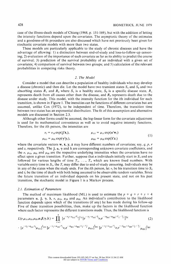
2. The Model Consider a model that can describe a population of healthy individuals who may develop a disease (chronic) and then die. Let the model have two transient states S1 and S2 and two absorbing states R1 and R2 where S1 is a healthy state, S2 is a specific disease state, R1 represents death from all causes other than the disease, and R2 represents death due to the disease under study. This model, with the intensity function for the ith individual for each transition, is shown in Figure 1. The inensities can be functions of diSerent covariates but are assumed, unlike Cox (1972), to be independent of time. Therefore, the transition time between two states has an exponential distribution. The fit of this assumption and alternative models are discussed in Section 2.3. Although other forms could be assumed, the log-linear form for the covariate adjustment is used for its mathematical convenience as well as to avoid negative intensity functions. Therefore, for the ith person, the intensities are

Vi = ^12 exp('Xi), glli = 811 exp(e'Wi) (1)

821i = 821 eXP(8'Yi), 822i = 822 eXP(A'Zi)

where the covariate vectors w, x, y, z may have different numbers of covariates; say, q, p, r and s, respectively. The 0, a, z and A are corresponding unknown covariate coefficients, and the v, ,u11, 821 and 822 are the respective underlying intensities when the covariates have no eSect upon a given transition. Further, suppose that n individuals initially start in S1 and are followed for various lengths of time T1, ..., Tn which are known fixed numbers. With variable entry time in S1, the Ti may diSer due to end-of-study censoring. Individuals may be in any of the states when the study ends. For the ith person, let ri be his transition time to S2 and ti be the time of death with both being assumed to be observable r andom variables. Since the future transition of an individual depends on his present state, and not on his past transition, the stochastic model in Figure 1 is a Markov process.

2.1. Estimation of Parameters The method of maximum likelihood (ML) is used to estimate the p + q + r + s + 4 parameters a, , , A, IJ, ,u11, 812 and 822@ An individual's contribution to the likelihood function depends upon which of the transitions (if any) he has made during his follow-up Five of these transition possibilities, then, make up the factors in the likelihood function where each factor represents the diSerent transitions made. Thus, the likelihood function is

n

L(v,H11,H21,y22,ct,d,t,) = tI [e-'l'i+81li'7i]6li [e-'Pi+8lli'Tivie-'821i+822i'(7i- Ti']e2i (2) i =1

Hllz] [e li ivie 21E+822i9'tz- Tz'g21z]621z [e- tt'i+Stllz) Ti - (At +At )(t - T



429 STOCHASTIC SURVIVAL MODELS WITH COVARIATES

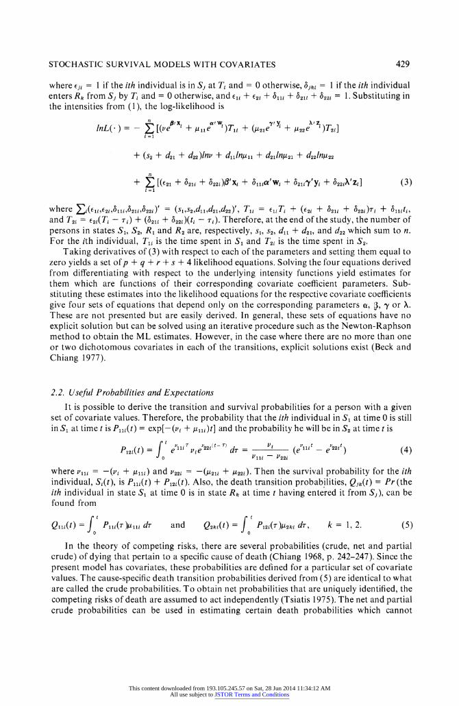
where fyi = 1 if the ith individual is in Sj at Ti and = O otherwise, ajki = 1 if the ith individual enters Rk from Sj by Ti and = O otherwise, and eli + 62i + alli + 621i + 622i = 1. Substituting in the intensities from (1), the log-likelihood is

lnL( ) =- fi [(, 'Xi + gl1e Wi)T15 + (M2le Yi + ,u22e i)T2X] i =1

+ (52 + d21 + d22)lnv + d1llngll + d21lny2l + d22lng22

n

+ A£, [(621 + 621i + 622i)13 XE + allE(t WE + 621it yi + 622iX Zi] (3) i =1

where ¢i((lis(2i,611i,621i622i)t = (Sl,S2,dll,d2l,d22)', Tli = eliTi + (62i + 621i + 622i)7i + allitis

and T2z = 62i(Ti - ti) + (6215 + 6225)(ti - Ti)- Therefore, at the end of the study, the number of persons in states S1, S2, R1 and R2 are, respectively, 51, 52 d1l + d21, and d22 which sum to n. For the ith individual, T1i is the time spent in S1 and T2i is the time spent in S2.

Taking derivatives of (3) with respect to each of the parameters and setting them equal to zero yields a set of p + q + r -t s + 4 likelihood equations. Solving the four equations derived from differentiating with respect to the underlyirlg intensity functions yield estimates for them which are functions of their corresponding covariate coefficient parameters. Sub- stituting these estimates into the likelihood equations for the respective covariate coefficients give four sets of equations that depend only on the corresponding parameters a, , z or A. These are not presented but are easily derived. In general, these sets of equations have no explicit solution but can be solved using an iterative procedure such as the Newton-Raphson method to obtain the ML estimates. However, in the case where there are no more than one or two dichotomous covariates in each of the transitions, explicit solutions exist (Beck and Chiang 1977).

2.2. Useful Probabilities and Expectations It is possible to derive the transition and survival probabilities for a person with a given

set of covariate values. Therefore, the probability that the ith individual in S1 at time O is still in S1 at time t is Pl1z(t) = expt-(vi + ,ul1E)t] and the probability he will be in S2 at time t is

Pl2E(t) = S elli vie22i' > dT = _i (e 11' - e22i ) (4)

where v1li =-(vi + ,ulli) and V22i =-(,U21g + ,U22E). Then the survival probability for the ith individual, Si(t), is P1li(t) + P12g(t). Also, the death transition probabilities, Qyk(t) = Pr (the ith individual in state S1 at time O is in state Rk at time t having entered it from Sj), can be found from

Qlli(t, = Q Plli(T)8lli dT and 02ki(t) = S P12z(T)82ki dTu k = 1, 2. (5)

In the theory of competing risks, there are several probabilities (crude, net and partial crude) of dying that pertain to a specific cause of death (Chiang 19689 p. 242-247). Since the present model has covariates, these probabilities are defined for a particular set of covariate values. The cause-specific death transition probabilities derived from (5) are identical to what are called the crude probabilities. To obtain net probabilities that are uniquely identified, the competing risks of death are assumed to act independently (Tsiatis 1975). The net and partial crude probabilities can be used in estimating certain death probabilities which cannot



430 BIOMETRICS, JUNE 1979

normally be observed but are calculated through their relationships with the crude probabilities. For example, it is meaningful to ask in the present model how the probability of dying is changed if the risk of dying from the disease (state S2) is eliminated. For a model with only two death states, this probability is both a net probability and a partial crude probability. Estimates of the competing risks probabilities can be obtained by substituting the parameter estimates into the appropriate probability expression.

The time of transition to S2, , and the death time, t, are random variables whose expectations can be calculated for a given set of covariate values. For t, which is also the survival time, one can get the probability distribution function of t from 1-Si(t), where Si(t) is the survival probability for the zth individual with his covariate values. Then the expectation of t follows. For , the probability density function for the ith person is Plli(T)lJi

and the expectation of r can be derived. The expected duration of stay in each state for an individual with certain covariates and who starts in S1 can also be calculated.

2.3. Other Models The model given in Figure 1 can be modified to fit other data situations. The first obvious

change is that the covariate adjustment need not be made on all transitions and that some of the covariate vectors may be the same; for example, w = x and y = z. Thus the number of parameters may be reduced (see Section 4 for an example). Another modification is to have more than the two competing death states. Transitions from both S1 and S2 into these additional states would be allowed and the intensity functions could depend upon covariates. For each additional transition, the likelihood function in (2) would be changed to include an additional factor that would represent the probability of someone starting in S1 and then making the transitions through this new one. If one of the additional death states is defined as "lost from observation", then individuals who are in either S1 or S2 and get lost can be handled as a competing risk by having them make the transition to this "death" state. The assumed independence of this state from the other death states must be considered.

Another important extension would be to allow reverse transitions in the model. For example, if S1 is also remission from disease S2 then the transition from S2 to S1 may be needed. However, a person in S1 after being in S2 may not have the same transition probability of moving to S2 as someone in S1 who has never been in S2. To accommodate this situation and since reverse transitions are not allowed in our models, we can define a new state S3 which would be defined as remission after being in S2 and a state S4 that is development of the disease after one remission. Then transitions from S3 and S4 to appropriate death states can be included in the model. If many remissions are possible such an extension to further states would become unwieldy and require more data to estimate the

Vj

sl 3 s2

821i / ,6tlli / 822i

vZ v R1 R2

Figure 1 A stochastic model with two transient and two absorbing states and intensity functions for the ith

individual .



STOCHASTIC SURVIVAL MODELS WITH COVARIATES 431

additional parameters. Such an approach has been taken by Chiang (1979) but without covariates.

The assumption that the transition times, Tt, from Sl to S2 are known can be relaxed. If it is known at the end of follow-up whether an individual is in S2 or a death state but not when he first entered S2, the contribution of that individual to the likelihood function can be changed. For persons ending in S2, their contributions become Pl2f(Ti), which was defined in (4). For persons ending in death state Rk, their contributiorls take the form Pl2z(ti)g2ki where 82ki iS the intensity for making the transition from S2 to Rk and may depend upon covariates similar to the form given in (1).

Another assumption made is that the transition intensity functions are time independent. For a given set of data, this assumption can be checked. Consider the transition from S1 to S2 where for now we assume the intensity is not a function of covariates. A plot of the logarithm of the probability of not making this transition at time Ti against UTi (the estimated cumulative intensity), where the Ti are the ordered transition times of persons entering S2, will give a straight line with a slope of-1 and an intercept of 0 if the assumption is correct. The probabilities can be estimated by the method of Kaplan and Meier (1958) where persons staying in S1 or making a transition to some state other than S2 are considered censored. In the case where a transition depends on the covariates (say, from S2 to R1), a similar plot can be made except that the estimated cumulative intensities are ,u2lti exp('yi). These then are ordered and plotted against the probabilities of not making the transition with the expected line having a slope of -1 and an intercept of 0. The cumulative intensities are equivalent to residuals which have a unit exponential distribution and the above process is an application of the general theory of residuals of Cox and Snell (1968).

If the time independence assumption is not met, one alternative is to divide the length of follow-up into intervals where each interval has its own constant intensity and which then allows covariates to change over time (see Holford 1976). Another possibility is to let the transition times for each transition follow a Weibull distribution that also depends upon covariates. For example, for the transition S1 to S2, the intensity for the ith individual with covariates xi would be v exp(0'x) ata- 1 where a is an additional parameter and t is time in S1. In fact, a model could contain a mixture of exponential and Weibull transitions. Any of these more general models involve more complex likelihood functions but the parameter estimates can be obtained as for the model in Figure 1.

3. Asymptotic Theory and Tests of Hypotheses

When the ML estimates are calculated from observing a number of independent and identically distributed random variables which satisfy certain regularity conditions, the ML estimates possess certain asymptotic properties, including having a normal distribution. However, the observations in the stochastic models presented here are independent but not identically distributed. This is for two reasons. Since the potential observation times, Ti, of the i = 1, 2, ..., n individuals are diSerent, the random variables ti have nonidentical distributions for those individuals who do not die before the end of their observation period Ti. The second reason is that each individual has his own set of covariate values which enter into his contribution to the likelihood function. Hence, satisfying the usual regularity conditions does not imply the standard asymptotic properties of ML estimates.

There exist, however, other regularity conditions for the independent and not identically distributed case so that asymptotic consistency and normality hold. One set of conditions has been given by Hoadley (1971), while others have been given by Bradley and Gart (1962) and Philippou and Roussas (1973). For the model in Figure 1 and similar models, each of these



432 BIO METRICS, JUN E 1979

diSerent sets of conditions are more restrictive than necessary and difficult to verify. Alterna- tively, the asymptotic normality of the ML estimates can be shown by meeting certain conditions for the terms in the expression of the logarithm of the likelihood ratio

A(0o + ^, b) = In[L(00 + b)/L(0o)] (6)

where 00 is a vector of the true parameter values and b has appropriate small increments about the true values. Specifically, this involves demonstrating that sequences of distributions under (00 + b) and (00) that arise out of (6) are contiguous, which is used to show that the third order terms of b converge to zero so that only the behavior of the first and second order terms needs to be examined along with the global property of consistency. This has been done for a model similar to the one in Figure 1 (see Beck 1975). Other approaches which have been used to show the asymptotic properties of Cox's model (e.g., Tsiatis 1978) may also be applicable to models such as in Figure 1.

Let all the parameters in a model be denoted by the vector 0(e.g., in the model in Figure 1, 0t - (^, 811, 821, 822, t, 0t, Vt, 2t). Therefore, the ML estimates of 0, given by 0, have a multivariate normal distribution with mean o and a variance-covariance matrix, I-1(o), whose inverse has js kth element

Ijk =-E [ af} a ( )2 (7)

The estimated variances and covariances are obtained by substituting the o for o in I(o) and finding I-1(o). The needed expectations are easily found except for cases where the ri are unknown for some individuals or if the ri are unknown for persons who die. In these cases, one can use the expression in (7) without the expectation for the j7 kth element of I(o) since these terms will converge asymptotically to their respective expectations.

In order to evaluate the importance of each covariate as far as its ability to influence the course of survival, tests of hypotheses can be performed on the covariate coefficient parameters. For this purpose there are various test statistics which have the same asymptotic chi- square distribution under standard regularity conditions (see Rao 1965, p. 349). The most common one is the likelihood ratio test statistic, while for testing whether individual covariates are significant, the parameter estimate divided by its standard deviation is more readily used. These hypotheses can be used to identify which covariates are significant and should be retained in the model. An important special case occurs when one wants to compare the survival of two (or three) groups of individuals. This can de done by defining one (or two) dichotomous covariates to indicate group membership, and then testing its (their) significance to determine whether the groups diSer.

d. Example To illustrate the use of these modeis, a two death state model as in Figure 1 has been

applied to analyze survival of patients in a heart transplant study. The data come from the Stanford Heart Transplant Program and have been analyzed by Crowley and Hu (1977) using the techniques of Cox (1972) and by others.

Briefly, patients with heart illnesses are admitted into the program after it is decided that their response to other forms of therapy would be negligible. Then a donor heart is sought for the patient. The donor and patient are matched closely by blood type and other criteria. Some patients have waited almost a year for a new heart. Consequently, a patient may die before receiving a heart, while those who receive a transplant may die from rejection of the new heart or from other causes. To evaluate this survival process the stochastic model in Figure 1 is used where the states are S1 accepted into the program, S2 received a new




heart, R2 died from rejecting the donor heart, and R1 died from any other cause. This model allows (as opposed to Crowley and Hu 1977) the data to be studied in one analysis that permits the death of transplanted patients to be analyzed by cause of death and allows diCerent covariates for each transition.

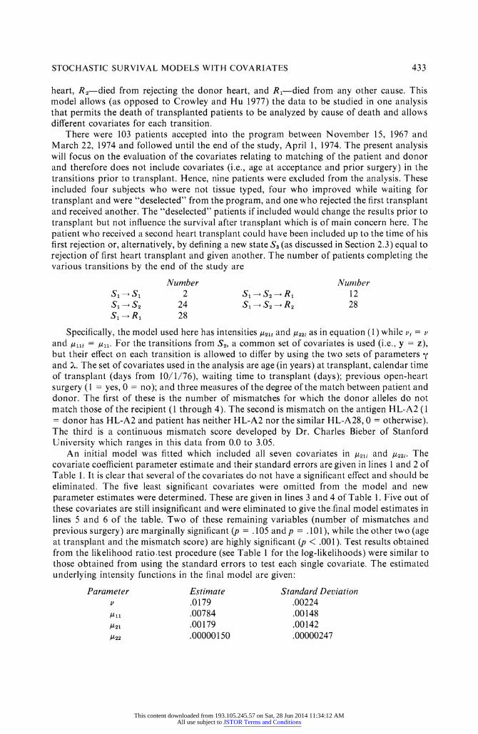
Therewere 103 patients accepted into theprogram between November 15, 1967 and March 22, 1974 and followed until the end of the study, April 1, 1974. The present analysis will focus on the evaluation of the covariates relating to matching of the patient and donor and therefore does not include covariates (i.e., age at acceptance and prior surgery) in the transitions prior to transplant. Hence, nine patients were excluded from the analysis. These included four subjects who were not tissue typed, four who improved while waiting for transplant and were 6'deselected" from the program, and one who rejected the first transplant and received another. The "deselected" patients if included would change the results prior to transplant but not influence the survival after transplant which is of main concern here. The patient who received a second heart transplant could have been included up to the time of his first rejection or, alternatively, by defining a new state S3 (as discussed in Section 2.3) equal to rejection of first heart transplant and given another. The number of patients completing the various transitions by the end of the study are

Number Number S1S1 2 SlS2Rl 12

S1 S2 24 S1 S2 R2 28

S1R1 28

Specifically7 the model used here has intensities ,u21i and y22i as in equation (1) while ri = U

and ,ulli = ,u11. For the transitions from S2, a common set of covariates is used (i.e.S Y = Z), but their eSect on each transition is allowed to diSer by using the two sets of parameters Py and A. The set of covariates used in the analysis are age (in years) at transplant, calendar time of transplant (days from 10/1/76), waiting time to transplant (days); previous open-heart surgery (1 = yes, 0 = no); and three measures of the degree of the match between patient and donor. The first of these is the number of mismatches for which the donor alleles do not match those of the recipient (1 through 4). The second is mismatch on the antigen HL-A2 (1 = donor has HL-A2 and patient has neither HL-A2 nor the similar HL-A28, 0 = otherwise). The third is a continuous mismatch score developed by Dr. Charles Bieber of Stanford University which ranges in this data from 0.0 to 3.05.

An initial model was fitted which included all seven covariates in 821i and 822i. The covariate coefficient parameter estimate and their standard errors are given in lines 1 and 2 of Table 1. It is clear that several of the covariates do not have a significant efTect and should be eliminated. The five least significant covariates were omitted from the model and new parameter estimates were determined. These are given in lines 3 and 4 of Table 1. Five out of these covariates are still insignificant and were eliminated to give the final model estimates in lines 5 and 6 of the table. Two of these remaining variables (number of mismatches and previous surgery) are marginally significant (p = .105 andp = .101), while the other two (age at transplant and the mismatch score) are highly significant (p < .001). Test results obtained from the likelihood ratio.test procedure (see Table 1 for the log-likelihoods) were similar to those obtained from using the standard errors to test each single covariate. The estimated underlying intensity functions in the final model are given:

Parameter Estimate Standard Deviation v .0179 .00224 g11 .00784 .00148 821 .00 l 79 .00142 822 .00000 l 50 .00000247



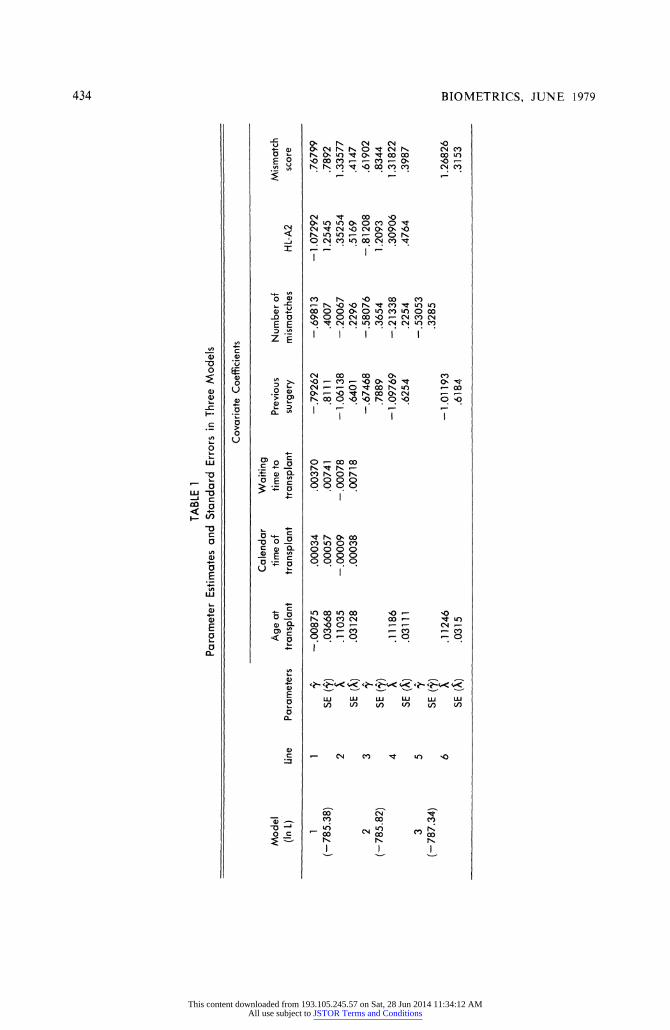
TABLE 1 Parameter Estimates and Standard Errors in Three AQodels

Covariate Coefficients

Calendar Waiting Model Age at time of time to Previous Number olF Mismatch (In L) Line Parameters transplant transplant transplant surgery mismatches HL-A2 score

1 1 z - .00875 .00034 .00370 -.79262 -.69813 - 1.07292 .76799 (-785.38) SE (z) .03668 .00057 .00741 .8111 .4007 1.2545 .7892

2 2 .11035 -.00009 -.00078 - 1.06138 - .20067 .35254 1.33577 SE (X) .03128 .00038 .00718 .6401 .2296 .5169 .4147

2 3 z -.67468 -.58076 -.81208 .61902 (-785.82) SE (#y) .7889 .3654 1.2093 .8344

4 2 .11186 - 1.09769 -.21338 .30906 l .31822 SE (X) .03111 .6254 .2254 .4764 .3987

3 5 z -.53053 (-787.34) SE (z) .3285

6 2 .11246 - 1.01193 1.26826 SE (X) .0315 .6184 .3153

_t

o

_t

ct -

llJ




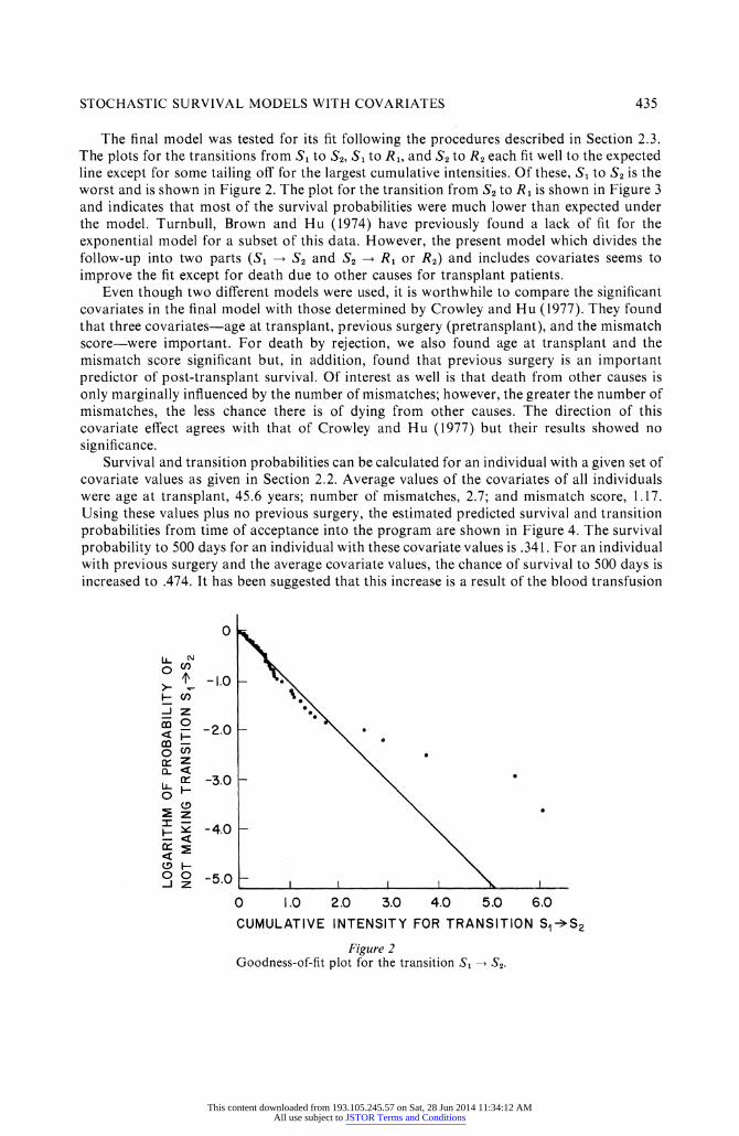
The final model was tested for its fit following the procedures described in Section 2.3. The plots for the transitions from S1 to S2, S1 to R1, and S2 to R2 each fit well to the expected line except for some tailing oF for the largest cumulative intensities. Of these, S1 to S2 is the worst and is shown in Figure 2. The plot for the transition from S2 to R1 is shown in Figure 3 and indicates that most of the survival probabilities were much lower than expected under the model. Turnbull, Brown and Hu (1974) have previously found a lack of fit for the exponential model for a subset of this data. However, the present model which divides the

follow-up into two parts (S1 S2 and S2 R1 or R2) and includes covariates seems to

improve the fit except for death due to other causes for transplant patients. Even though two diSerent models were used, it is worthwhile to compare the significant

covariates in the final model with those determined by Crowley and Hu (1977). They found that three covariates age at transplant, previous surgery (pretransplant), and the mismatch score were important. For death by rejection, we also found age at transplant and the mismatch score significant but, in addition, found that previous surgery is an important predictor of post-transplant survival. Of interest as well is that death from other causes is only marginally inRuenced by the number of mismatches; however, the greater the number of mismatches, the less chance there is of dying from other causes. The direction of this covariate efTect agrees with that of Crowley and Hu (1977) but their results showed no

. .

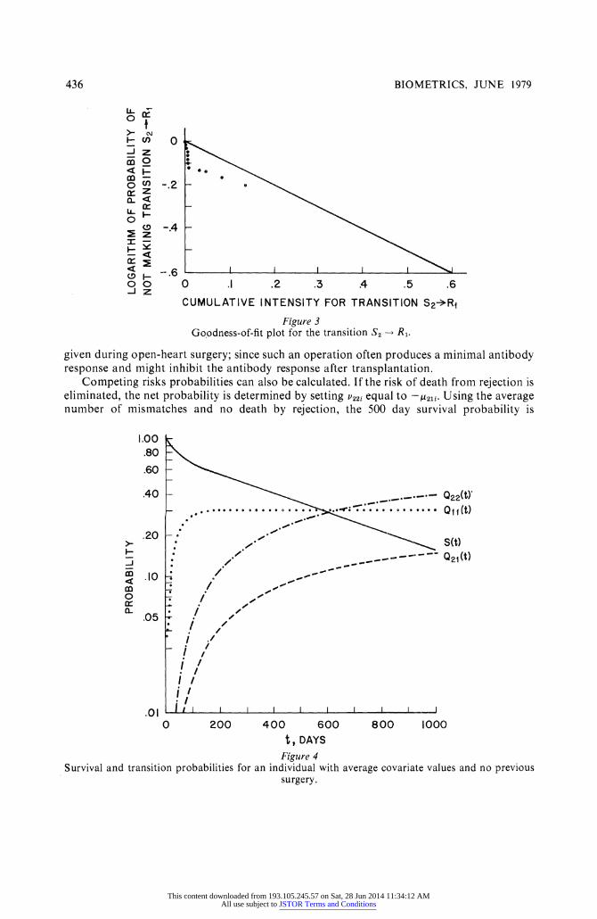
slgnlacance. Survival and transition probabilities can be calculated for an individual with a given set of

covariate values as given in Section 2.2. Average values of the covariates of all individuals were age at transplant, 45.6 years; number of mismatches, 2.7; and mismatch score, 1.17. Using these values plus no previous surgery, the estimated predicted survival and transition probabilities from time of acceptance into the program are shown in Figure 4. The survival probability to 500 days for an individual with these covariate values is .341. For an individual with previous surgery and the average covariate values, the chance of survival to 5QQ days is increased to .474. It has been suggested that this increase is a result of the blood transfusion

04 LLCQ \

F cn za J z *0\

< ° - 2 0 - )\ \

O O \ O cK z \

.L F 3 ° - \ e

5; z \ F

F Y -4.0 - \ _ < \

zr \

° z 5.0 1 1 1 1 \ 2

O 1.0 2.0 3.0 4.() 5.0 6.0 CUMULATIVE INTENSITY FOR TRANSITION S1 + S2

Figure 2

Goodness-of-fit plot for the transition S1 S2.



.. . .


o f > CQ

n

Z m °

m i o cn

Z

_

o

Z

I - - <

cK

O O I Z

o

.2

-.4

-- .6 O .1 .2 .3 .4 .5 .6

CUMULATIVE INTENSITY FOR TRANSITION Sa+R

Figure 3

Goodness-of-fit plot for the transition S2 R1.

given during open-heart surgery; since such an operation often produces a minimal antibody response and might inhibit the antibody response after transplantation.

Competing risks probabilities can also be calculated. If the risk of death from rejection is eliminated, the net probability is determined by setting p22i equal to -821i Using the average number of mismatches and no death by rejection, the 500 day survival probability is

1.00

.80

.60

.40

- 0_-0-0 Q22(t)

e o 0 0 0 0 0 e @ e @ @ @ o e ; * * X * @ @ * @ ° Q 1 t (t)

,@° S(t)

. / _ __- - Q2, (t) - / _ , S o

.20

.10

.05

m

m o CK L

- / woD * * /

} / * / /

b * /

T ! o' . , ,

s , ,

, ., _ ,

1,

j, * ,

, i ' .,

l l l l

.01 200 400 600 800 1000

t, DAYS

Figure 4 Survival and transition probabilities for an individual with average covariate values and no previous

surgery.



437 STOCHASTIC SURVIVAL MODELS WITH COVARIATES

increased to .572. Therefore, if death by rejection from receiving a new heart can be reduced, the prognosis of patients can be improved although the amount of improvement given here assumes independent risks of death and that the model fits. In summary, the method of analysis given here oWers the advantages of evaluating survival by cause of death and calculating competing risks probabilities, but suffers in this example from a lack of fit for the transition 2 to R1. This possibly could be overcome by dividing the follow-up time into intervals.

A cknowledgenents I wish to thank Professor C. L. Chiang for his helpful guidance in this research and Professors L. Le Cam, R. Barlow, and R. Beran for their invaluable comments. Useful comments by the editor, associate editor, and referees have also been incorporated into the paper. Computer support and miscellaneous research expenses were provided in part through General Research Support GraIlt 5-501-RR-05441 from the National Institutes of Health, U.S. Department of Health, Education and Welfare to the School of Public Health, University of (California at Berkeley.

Resuene En analyse de survie, l'inforszation des covariables a ete utilisee pour evaluer leur importance dans la prediction de la probabilite' de survie d'un individu donne'. Cet article de'veloppe un modele ale'atoire de survie incorporant des covariables et comprenant deux etats de sante et plusieurs risques simultane's. Les fonctions d'intensite' de transition peuvent avoir une forme exponentielle ou de Weibull mais de'pendent des covariables. On pre'sente d'autres gene'ralisations du modele. Le modele de Lagakos (1976) est un cas particulier des modeles propose's ici. La theorie asymptotique des estimateurs du maximum de vraisemblance et une procedure d'ajustement sont discute'es, ainsi que l'estimation des probabilites de survie, de transition et des risques simultane's. Ces modeles sont applicables a des donne'es recueillies dans un essai clinique ou une etude prospective et peuvent distinguer une e'tude termine'e ou une enquezte inacheve'e. On donne une application a' l'analyse de la survie de patients d'un programme de transplantation cardiaque.

R eferences Beck, G. J. (1975). Stochastic survival models with competing risks and covariates. Unpublished Ph.D. dissertation, University of California, Berkeley, California. Beck, G. J. and Chiang, C. L. (1977). Explicit maximum likelihood solutions for stochastic survival models with one or two dichotomous covariates. Paper presented at the joint meetings of the Biometric Society (ENAR) and the American Statistical Association, Chapel Hill, North Caro- lina. Biometrics Abstract 2471. Bradleyy R. A. and Garty J. J. (1962). The asymptotic properties of ML estimators when sampling from associated populations. Biometrika 49, 205-214. Chiang, C. L. (1968). Introduction to Stochastic Processes in Biostatistics. John Wiley and Sons, Inc., New York. Chiang, C. L. (1979). Survival and stages of disease. To appear in Mathematical Biosciences. Cox, D. R. and Snell, E. J. (1968). A general definition of residuals. Journal of the Royal Statistical Society, Series B 30, 248-275. Cox, D. R. (-1972). Regression models and life-tables (with discussion). Journal of the Royal Statistical Society, Series B 34, 187-220. Crowley, J. and Hu, M. (1977). Covariance analysis of heart transplant survival data. Journal of the A merican Statistical A ssociation 72, 27-36. Feigl, P. and Zelen, M. (1965). Estimation of exponential survival probabilities with concomitant information. Biometrics 21, 826-838.




Hoadley, B. (1971). Asymptotic properties of maximum likelihood estimators for the independent not identically distributed case. Annals of Mathematical Statistics 42, 1977-1991.

Holford, T. R. (1976). Life tables with concomitant information. Biometrics 32, 587-597. Kaplan, E. L. and Meier, P. (1958). Nonparametric estimation from incomplete observations. Journal

of the American Statistical Association 53, 457-481. Lagakos, S. W. (1976). A stochastic model for censored survival data in the presence of an auxiliary

variable. Biometrics 32, 551-559. Philippou, A. N. and Roussas, G. G. (1973). Asymptotic distribution of the likelihood function in the

independent not identically distributed case. The Annals of Statistics 1, 454-471. Rao, C. R. (1965). Linear Statistical Inference and Its Applications. John Wiley and Sons, Inc., New

York. Tsiatis, A. (1975). A nonidentifiability aspect of the problem of competing risks. Proceedings of the

National Academy of Science 72, 20-22. Tsiatis, A. (1978). A large sample study of the estimate for the integrated hazard function in Cox's

regression model for survival data. Technical Report No. 526, Department of Statistics, University of Wisconsin, Madison, Wisconsin.

Turnbull, B. W., Brown, B. W., Jr. and Hu, M. (1974). Survivorship analysis of heart transplant data. Journal of the American Statistical Association 69, 74-80.

Received September 1977; Revised June 1978 and November 1978



Documents

Stochastic Survival Models with Competing Risks and Covariates