Embed Size (px)
Citation preview
Stochastic Subgradient Methods
Yu-Xiang WangCS292F
(Based on Ryan Tibshirani’s 10-725)
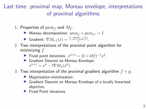
Last time: proximal map, Moreau envelope, interpretationsof proximal algorithms
1. Properties of proxf and Mf .I Moreau decomposition: proxf + proxf∗ = I.
I Gradient: ∇Mt,f (x) =x−proxt,f (x)
t .
2. Two interpretations of the proximal point algorithm forminimizing fI Fixed point iterations: xk+1 = (I + t∂f)−1xk.I Gradient Descent on Moreau Envelope:
xk+1 = xk − t∇Mf (xk).
3. Two interpretation of the proximal gradient algorithm f + g.I Majorization-minimization.I Gradient Descent on Moreau Envelope of a locally linearized
objective,I Fixed Point iterations
2

Outline
Today:
• Stochastic subgradient descent
• Convergence rates
• Mini-batches
• Early stopping
3
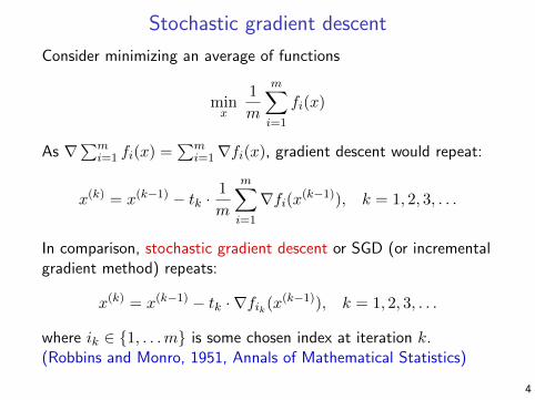
Stochastic gradient descent
Consider minimizing an average of functions
minx
1
m
m∑i=1
fi(x)
As ∇∑m
i=1 fi(x) =∑m
i=1∇fi(x), gradient descent would repeat:
x(k) = x(k−1) − tk ·1
m
m∑i=1
∇fi(x(k−1)), k = 1, 2, 3, . . .
In comparison, stochastic gradient descent or SGD (or incrementalgradient method) repeats:
x(k) = x(k−1) − tk · ∇fik(x(k−1)), k = 1, 2, 3, . . .
where ik ∈ {1, . . .m} is some chosen index at iteration k.(Robbins and Monro, 1951, Annals of Mathematical Statistics)
4

Two rules for choosing index ik at iteration k:
• Randomized rule: choose ik ∈ {1, . . .m} uniformly at random
• Cyclic rule: choose ik = 1, 2, . . .m, 1, 2, . . .m, . . .
Randomized rule is more common in practice. For randomized rule,note that
E[∇fik(x)] = ∇f(x)
so we can view SGD as using an unbiased estimate of the gradientat each step
Main appeal of SGD:
• Iteration cost is independent of m (number of functions)
• Can also be a big savings in terms of memory useage
5
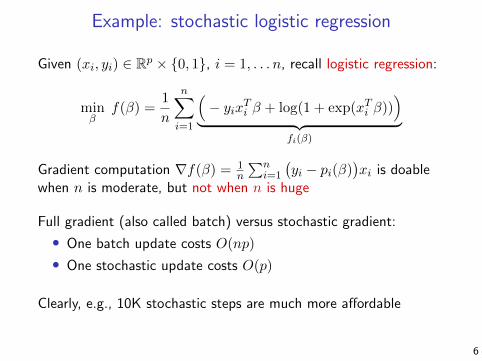
Example: stochastic logistic regression
Given (xi, yi) ∈ Rp × {0, 1}, i = 1, . . . n, recall logistic regression:
minβ
f(β) =1
n
n∑i=1
(− yixTi β + log(1 + exp(xTi β))
)︸ ︷︷ ︸
fi(β)
Gradient computation ∇f(β) = 1n
∑ni=1
(yi − pi(β)
)xi is doable
when n is moderate, but not when n is huge
Full gradient (also called batch) versus stochastic gradient:
• One batch update costs O(np)
• One stochastic update costs O(p)
Clearly, e.g., 10K stochastic steps are much more affordable
6
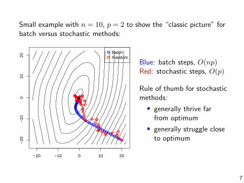
Small example with n = 10, p = 2 to show the “classic picture” forbatch versus stochastic methods:
−20 −10 0 10 20
−20
−10
010
20
●●●●●●●●●●●●●●●●●●●●●●●●●●●
●●●●●●●●●●●●●●●●●●●●●●●
●●●
●●
●●
●●●
●●●
●●●
●
●●●●
●●
●●●●
●
●●●●
●●●●●
●● ●●●●●●
●●●
●●*
●
●
BatchRandom
Blue: batch steps, O(np)Red: stochastic steps, O(p)
Rule of thumb for stochasticmethods:
• generally thrive farfrom optimum
• generally struggle closeto optimum
7
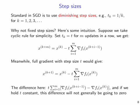
Step sizes
Standard in SGD is to use diminishing step sizes, e.g., tk = 1/k,for k = 1, 2, 3, . . .
Why not fixed step sizes? Here’s some intuition. Suppose we takecyclic rule for simplicity. Set tk = t for m updates in a row, we get:
x(k+m) = x(k) − tm∑i=1
∇fi(x(k+i−1))
Meanwhile, full gradient with step size t would give:
x(k+1) = x(k) − tm∑i=1
∇fi(x(k))
The difference here: t∑m
i=1[∇fi(x(k+i−1))−∇fi(x(k))], and if wehold t constant, this difference will not generally be going to zero
8
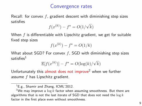
Convergence rates
Recall: for convex f , gradient descent with diminishing step sizessatisfies
f(x(k))− f? = O(1/√k)
When f is differentiable with Lipschitz gradient, we get for suitablefixed step sizes
f(x(k))− f? = O(1/k)
What about SGD? For convex f , SGD with diminishing step sizessatisfies1
E[f(x(k))]− f? = O(log(k)/√k)
Unfortunately this almost does not improve2 when we furtherassume f has Lipschitz gradient.
1E.g., Shamir and Zhang, ICML’2012.2We may improve a log k factor when assuming smoothness. But there are
algorithms that is not the last iterate of SGD that does not need the log kfactor in the first place even without smoothness.
9
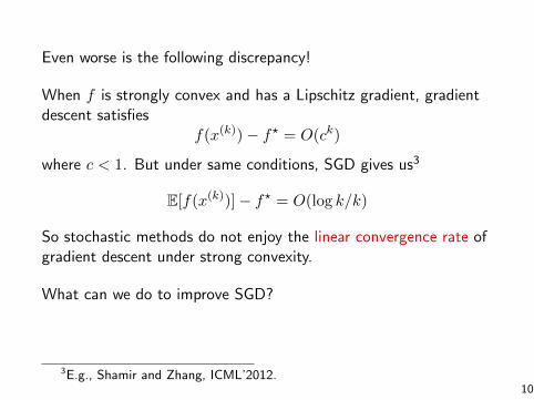
Even worse is the following discrepancy!
When f is strongly convex and has a Lipschitz gradient, gradientdescent satisfies
f(x(k))− f? = O(ck)
where c < 1. But under same conditions, SGD gives us3
E[f(x(k))]− f? = O(log k/k)
So stochastic methods do not enjoy the linear convergence rate ofgradient descent under strong convexity.
What can we do to improve SGD?
3E.g., Shamir and Zhang, ICML’2012.10
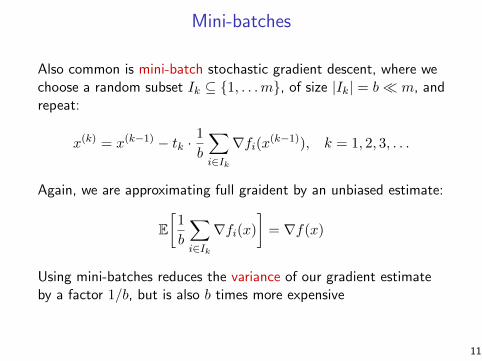
Mini-batches
Also common is mini-batch stochastic gradient descent, where wechoose a random subset Ik ⊆ {1, . . .m}, of size |Ik| = b� m, andrepeat:
x(k) = x(k−1) − tk ·1
b
∑i∈Ik
∇fi(x(k−1)), k = 1, 2, 3, . . .
Again, we are approximating full graident by an unbiased estimate:
E[
1
b
∑i∈Ik
∇fi(x)
]= ∇f(x)
Using mini-batches reduces the variance of our gradient estimateby a factor 1/b, but is also b times more expensive
11
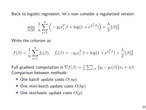
Back to logistic regression, let’s now consider a regularized version:
minβ∈Rp
1
n
n∑i=1
(− yixTi β + log(1 + ex
Ti β))
+λ
2‖β‖22
Write the criterion as
f(β) =1
n
n∑i=1
fi(β), fi(β) = −yixTi β + log(1 + exTi β) +
λ
2‖β‖22
Full gradient computation is ∇f(β) = 1n
∑ni=1
(yi− pi(β)
)xi +λβ.
Comparison between methods:
• One batch update costs O(np)
• One mini-batch update costs O(bp)
• One stochastic update costs O(p)
12

Example with n = 10, 000, p = 20, all methods use fixed step sizes:
0 10 20 30 40 50
0.50
0.55
0.60
0.65
Iteration number k
Crit
erio
n fk
FullStochasticMini−batch, b=10Mini−batch, b=100
13

What’s happening? Now let’s parametrize by flops:
1e+02 1e+04 1e+06
0.50
0.55
0.60
0.65
Flop count
Crit
erio
n fk
FullStochasticMini−batch, b=10Mini−batch, b=100
14

Finally, looking at suboptimality gap (on log scale):
0 10 20 30 40 50
1e−
121e
−09
1e−
061e
−03
Iteration number k
Crit
erio
n ga
p fk
−fs
tar
FullStochasticMini−batch, b=10Mini−batch, b=100
15

Convergence rate proofs
Algorithm: xk+1 = xk − tkgk.Assumptions: (1) Unbiased subgradient: E[gk|xk] ∈ ∂f(xk).(2) Bounded variance: E[‖gk − E[gk|xk]‖2|xk] ≤ σ2
• Convex and G-Lipschitz (Proof this!)
mini=1,...,k
E[f(xi)
]− f∗ ≤
‖x1 − x∗‖2 + (G2 + σ2)∑k
i=1 t2i
2∑k
i=1 ti
• Nonconvex but L-smooth with ti = 1/(√kL) (Proof this!)
E
[1
k
k∑i=1
‖∇f(xi)‖2]≤ 2(f(x1)− f∗)L+ σ2√
k
• m-Strongly convex and G-Lipschitz: O(G2 log(T )/mT ) rate.we will prove this when we talk about online learning!
16

Averaging Stochastic (Sub)gradient DescentOne drawbacks of SGD: the guarantees are formini=1,...,k E
[f(xi)
].
Idea: Let’s output the online averages of the iterates.
x̄k =k − 1
kx̄k−1 +
1
kxk(Polyak-Rupert Averaging)4
Convergence bound:
E[f(x̄k)]− f∗ ≤
{O(1/
√k) if convex (We just proved that!)5
O(log k/k) if strongly convex
Can the log k be removed? No. Use α-Suffix averaging. (Rakhlin,Shamir, Sridharan, ICML’2012)But that doesn’t have an online implementation. Solution by(Shamir and Zhang, ICML’2013) : x̄kη = (1− 1+η
k+η )x̄k−1η + 1+ηk+ηx
k.4See, Polyak,1990; Rupert,1988; Polyak and Juditsky, 1992.5Using ideas from Nemirovski et al. (2009).
17
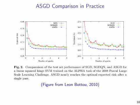
ASGD Comparison in Practice
(Figure from Leon Bottou, 2010)
18
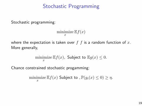
Stochastic Programming
Stochastic programming:
minimizex
Ef(x)
where the expectation is taken over f f is a random function of x.More generally,
minimizex
Ef(x), Subject to Eg(x) ≤ 0.
Chance constrained stochastic progamming:
minimizex
Ef(x) Subject to ,P(gi(x) ≤ 0) ≥ η.
19
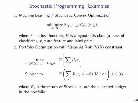
Stochastic Programming: Examples
1. Machine Learning / Stochastic Convex Optimization
minimizeh∈H
E(x,y)∼D[`(h, (x, y))]
where ` is a loss function, H is a hypothesis class (a class ofclassifiers), x, y are feature and label pairs.
2. Portfolio Optimization with Value At Risk (VaR) constraint.
maxx:x≥0,
∑i xi= Budget
E
[∑i
Rixi
],
Subject to P
(∑i
Rixi ≤ −$1 Million
)≤ 0.05
where Ri is the return of Stock i, xi are the allocated budgetin the portfolio.
20
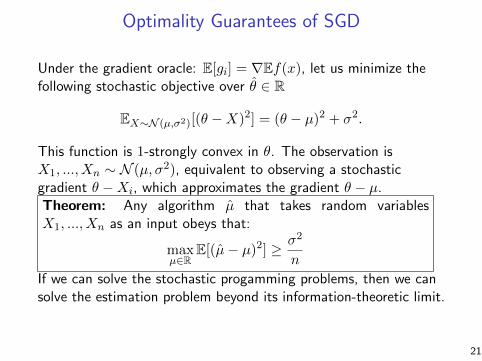
Optimality Guarantees of SGD
Under the gradient oracle: E[gi] = ∇Ef(x), let us minimize thefollowing stochastic objective over θ̂ ∈ R
EX∼N (µ,σ2)[(θ −X)2] = (θ − µ)2 + σ2.
This function is 1-strongly convex in θ. The observation isX1, ..., Xn ∼ N (µ, σ2), equivalent to observing a stochasticgradient θ −Xi, which approximates the gradient θ − µ.Theorem: Any algorithm µ̂ that takes random variablesX1, ..., Xn as an input obeys that:
maxµ∈R
E[(µ̂− µ)2] ≥ σ2
n
If we can solve the stochastic progamming problems, then we cansolve the estimation problem beyond its information-theoretic limit.
21

Optimality Guarantees of SGD
Similarly, consider
minθ∈[−1,1]
E[Xθ] = pθ − (1− p)θ = (−1 + 2p)θ
where P(X = 1) = p and P(X = −1) = 1− p.This is a convex and 1-Lipschitz objective. Observing samplesX1, ..., Xn from that distribution can be considered stochasticgradient.sStatistical lower bound 1/
√n on estimating p suggest that we
cannot distinguish between the world when p = 0.5− 1/√n and
the world when p = 0.5 + 1/√n, which implies a lower bound of
1/√k for the convergence rate of SGD for non-strongly convex
stochastic objective.
22

End of the story?Short story:
• SGD can be super effective in terms of iteration cost, memory• But SGD is slow to converge, can’t adapt to strong convexity• And mini-batches seem to be a wash in terms of flops (though
they can still be useful in practice)• Averaging trick helps to remove log k terms in cases without
smoothness.• Lower bound from stochastic programming that says 1/
√k is
optimal in general and 1/k for strongly convex.
Is this the end of the story for SGD?
For a while, the answer was believed to be yes. But this was for amore general stochastic optimization problem, wheref(x) =
∫F (x, ξ) dP (ξ).
New wave of “variance reduction” work shows we can modify SGDto converge much faster for finite sums (more later?)
23
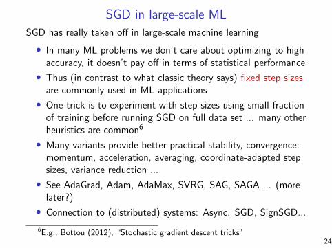
SGD in large-scale ML
SGD has really taken off in large-scale machine learning
• In many ML problems we don’t care about optimizing to highaccuracy, it doesn’t pay off in terms of statistical performance
• Thus (in contrast to what classic theory says) fixed step sizesare commonly used in ML applications
• One trick is to experiment with step sizes using small fractionof training before running SGD on full data set ... many otherheuristics are common6
• Many variants provide better practical stability, convergence:momentum, acceleration, averaging, coordinate-adapted stepsizes, variance reduction ...
• See AdaGrad, Adam, AdaMax, SVRG, SAG, SAGA ... (morelater?)
• Connection to (distributed) systems: Async. SGD, SignSGD...
6E.g., Bottou (2012), “Stochastic gradient descent tricks”24

Early stopping
Suppose p is large and we wanted to fit (say) a logistic regressionmodel to data (xi, yi) ∈ Rp × {0, 1}, i = 1, . . . n
We could solve (say) `2 regularized logistic regression:
minβ∈Rp
1
n
n∑i=1
(− yixTi β + log(1 + ex
Ti β))
subject to ‖β‖2 ≤ t
We could also run gradient descent on the unregularized problem:
minβ∈Rp
1
n
n∑i=1
(− yixTi β + log(1 + ex
Ti β))
and stop early, i.e., terminate gradient descent well-short of theglobal minimum
25
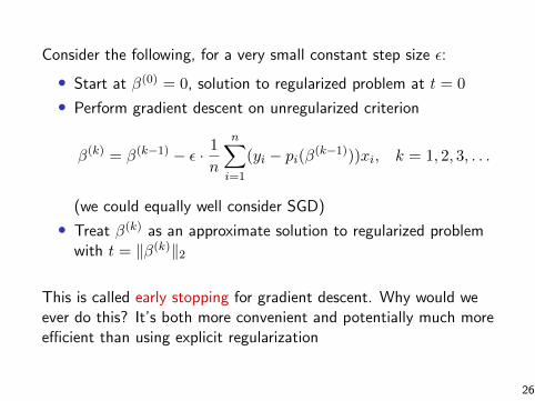
Consider the following, for a very small constant step size ε:
• Start at β(0) = 0, solution to regularized problem at t = 0
• Perform gradient descent on unregularized criterion
β(k) = β(k−1) − ε · 1
n
n∑i=1
(yi − pi(β(k−1)))xi, k = 1, 2, 3, . . .
(we could equally well consider SGD)
• Treat β(k) as an approximate solution to regularized problemwith t = ‖β(k)‖2
This is called early stopping for gradient descent. Why would weever do this? It’s both more convenient and potentially much moreefficient than using explicit regularization
26
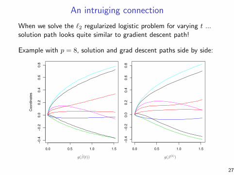
An intruiging connection
When we solve the `2 regularized logistic problem for varying t ...solution path looks quite similar to gradient descent path!
Example with p = 8, solution and grad descent paths side by side:
0.0 0.5 1.0 1.5
−0
.4−
0.2
0.0
0.2
0.4
0.6
0.8
Ridge logistic path
Co
ord
ina
tes
g(β̂(t))
0.0 0.5 1.0 1.5
−0.4
−0.2
0.0
0.2
0.4
0.6
0.8
Stagewise path
g(β(k))
Coor
din
ates
27
Lots left to explore
• Connection holds beyond logistic regression, for arbitrary loss
• In general, the grad descent path will not coincide with the `2regularized path (as ε→ 0). Though in practice, it seems togive competitive statistical performance
• Can extend early stopping idea to mimick a generic regularizer(beyond `2)7
• There is a lot of literature on early stopping, but it’s still notas well-understood as it should be
• Early stopping is just one instance of implicit or algorithmicregularization ... many others are effective in large-scale ML,they all should be better understood
7Tibshirani (2015), “A general framework for fast stagewise algorithms”28
References and further reading
• D. Bertsekas (2010), “Incremental gradient, subgradient, andproximal methods for convex optimization: a survey”
• A. Nemirovski and A. Juditsky and G. Lan and A. Shapiro(2009), “Robust stochastic optimization approach tostochastic programming”
• O. Shamir, T. Zhang. (2013). “Stochastic gradient descentfor non-smooth optimization: Convergence results andoptimal averaging schemes”. In International Conference onMachine Learning.
• R. Tibshirani (2015), “A general framework for fast stagewisealgorithms”
• Bernstein, W., Azizzadenesheli, and Anandkumar (2018).“signSGD: Compressed Optimisation for Non-ConvexProblems.”
29