Solar Energy. Vol. 23. pp. 47-51 0038-092X/7910701-0047/$02.00/0 © Pergamon Press Ltd.. 1979. Printed in Great Britain

STOCHASTIC SIMULATION OF HOURLY GLOBAL RADIATION SEQUENCES

CARLO MUSTACCHI, VINCENZO CENA and MASSIMO ROCCHi Istituto di Chimica Applicata e Industriale, Universith di Roma, Roma. Italia

(Received 7 November 1978; revision accepted 29 January 1979)

Abstract--Stochastic simulation of hourly global radiation carried out with Auto-Regressive Moving Average and Factor Analysis techniques is found unable to describe the statistical features of time sequences. A Markov transition-matrix approach operating on atmospheric transmittance provides a simple yet effective simulation device. Two novel sophisticated models, the transmittance transition tensor and the Gaussian mapping technique are not justified in this context.

l. INTRODUCTION

The thermal time constants of solar collectors range from a few minutes to a few hours, at most. Yet, for lack of suitable data on solar radiation transients, evaluations of these systems are often carried out on the basis of mean values of global radiation.

Since the response of the collectors to the wide fluctuations of radiation about the means can entail large variations in performance, a need is often felt for an appropriate model to generate solar radiation noise and thus simulate realistic operating conditions.

A number of possible models have been tested and evaluated; their structure is hereafter described and their limitations discussed.

2. DETRENDIZING RADIATION SEQUENCES

An insight is gained from a Fourier transform of the radiation sequences [I, 2]:

=f+° F(s) _® W ( t ) e x p ( - i s t ) d t (1)

which provides a description of the power spectrum. This spectrum exhibits a number of peaks due primarily to periodic circumstances, such as the regular succession of the seasons or of night and day. To avoid the burden of carrying along these low-frequency components, a procedure has to be chosen for cancelling from the data the effects of such a deterministic trend.

Three techniques have been experimented with in the course of this study:

(1) Subtraction from the radiation value of some means of the data, such as the average value of radiation at the same hour for each day of the same month or season.

(2) Subtraction or division of the data by radiation values obtained from a physical model which accounts for the extra-atmospheric radiation and for the ab- sorption and scattering effects of the atmosphere.

(3) Division of the data by the value of the extra- atmospheric radiation on a similarly oriented plane. The first detrendization technique, thought very satis- factory, is the least usuable, since it does not lend to

generalizations and requires an extended collection of hourly data at the location.

The second involves a knowledge of local instan- taneous values of turbidity, humidity, cloud type and frequency. Experiments carried out with the Dogniaux model[3], once acquired such data, were in very fair agreement with observations (relative standard deviation lower than l0 per cent). The third technique, although grossly neglecting the local climatic and meteorological effects, was finally adopted because it is the only one which can be practically used in the absence of data.

An apparent transmittance T of the atmosphere was thus obtained by dividing observed hourly radiation values by the values of the corresponding extra-atmos- pheric radiation [4].

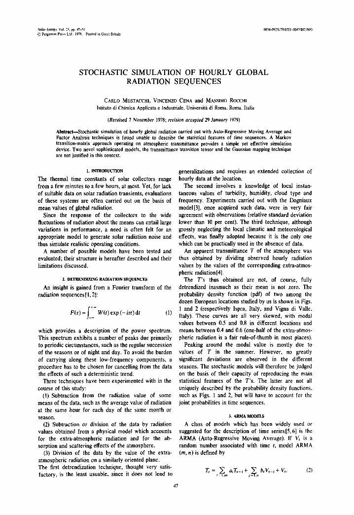
The T's thus obtained are not, of course, fully detrendized inasmuch as their mean is not zero. The probability density function (pdf) of two among the dozen European locations studied by us is shown in Figs. 1 and 2 (respectively Ispra, Italy, and Vigna di Valle, Italy). These curves are all very skewed, with modal values between 0.5 and 0.8 in different locations and means between 0.4 and 0.6 (one-half of the extra-atmos- pheric radiation is a fair rule-of-thumb in most places).

Peaking around the modal value is mostly due to values of T in the summer. However, no greatly significant deviations are observed in the different seasons. The stochastic models will therefore be judged on the basis of their capacity of reproducing the main statistical features of the T's. The latter are not all uniquely described by the probability density functions. such as Figs. 1 and 2, but will have to account for the joint probabilities in time sequences.

3. ARMA MODELS

A class of models which has been widely used or suggested for the description of time series[5,6] is the ARMA (Auto-Regressive Moving Average). If V, is a random number associated with time t, model ARMA (m, n) is defined by

T f = Z a i T t - i + Z b t V t - j + V t . (2) i = I .m j = I .n

47

48 C. MUSTACCHI et a l .

O

LOCATION A

o YEAR

÷ SUMMER ÷

A WINTER + ÷

A A + A ~

g" " '<3v-'r"4xZ"O,' ~ z x ~

0 61 0.2 013 014 0.5 0.6 O17 O:8 - 019 1.0

T

Fig. 1. Probability density function of atmospheric transmittance at location A (Ispra, Italy).

Using, as an example, a model ARMA (6, 0), the follow- ing values were obtained: Location A (Ispra)---al = 0.752; a2 = 0.060; a3 = 0.0005; a4 = 0.044; a5 = 0.010; a6 = 0.005. Location B (Vigna di Valle)---a j = 0.586; a2 = 0.078; a3 = 0.037; a4 = 0.022; a5 = 0.033; a6 = 0.018.

The low value of all the constants beyond a, shows that a model ARMA (1,0) or ARMA (2,0) is sufficient, if an auto-regressive description is accepted.

This result is similar to that found by[5] and [6] to describe, respectively, daily and hourly radiation sequences. The models turn to be: Location A

Tt = 0.759 T,_, + 0.096 T,-2 + V

were were V has a variance 0.133. Location B

T, =0.601 7",_, +0.127 T,-z+ V

where V as a variance 0.106. These expressions were used to compute, for a sample

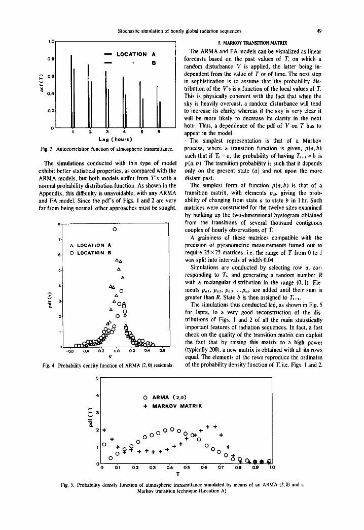
of about 8000 hourly measurements, the values of resi- duals V. Hystograms of such residuals, shown in Fig. 4, indicate that V is not a normal deviate. The distribution is bimodal and skewed. Chi-square tests whith any reason- able confidence level reject the possibility of generating V with a Gaussian algorithm.

Further, althougn the autocorrelation of residuals V showed these to be uncorrelated, they still retained a high degree of cross-correlation to the T's, thus in- validating the model.

4. FACTOR ANALYSIS

A more firmly based statistical procedure to construct solar sequences can be based upon the principal com- ponent method of Factor Analysis (FA)[7].

In essence, assuming that an ARMA (m, 0) expression holds, a search must be made on the redundancy of information carried by the n values of T in the previous times. New variables (the principal components) are constructed so that they are mutually orthogonal, and a linear regression is found by least squares linking Tr and the principal components.

This regression constitutes the "deterministic" part of the forecast. A check is then made on whether the residuals are still autocorrelated. This procedure yields a stable relation, which requires fewer observations than the ARMA models to converge to a statistically significant expression. Two eigenvalues of the cor- relation matrix (or principal components) were found to be sufficient in a dozen locations to account for over 90 per cent of the variance of T. It can be shown that the use of two components is equivalent to linearly relating 7", to the two variables Tr-j and (T,-I - T,-2).

~ ' 3. v

"O

2"

1"

0 0

LOCATION B + +

O YEAR

+ SUMMER + OO A WINTER

+o ~° + o + n

; , , , ,, T .. T + . . . .

O.1 0.2 0.3 0.4 0.5 0.6 0.7 0.8 0.9 1.0

T

Fig. 2. Probability density function of atmospheric transmittance at location B (Vigna di Valle, Italy),

Stochastic simulation of hourly global radiation sequences 49

1.0 5. MARKOV TRANSmON MATRIX

The ARMA and FA models can be visualized as linear LOCATION A o.a forecasts based on the past values of T, on which a

m a i m , , e

random disturbance V is applied, the latter being in- ~' o.e dependent from the value of T or of time. The next step HI II in sophistication is to assume that the probability dis-

tribution of the V's is a function of the local values of T. o.4 This is physically coherent with the fact that when the

sky is heavily overcast, a random disturbance will tend 0.2 to increase its clarity whereas if the sky is very clear it

will be more likely to decrease its clarity in the next hour. Thus, a dependence of the pdf of V on T has to

4 s e appear in the model. k a 9 ( h o u r s ) ' The simplest representation is that of a Markov

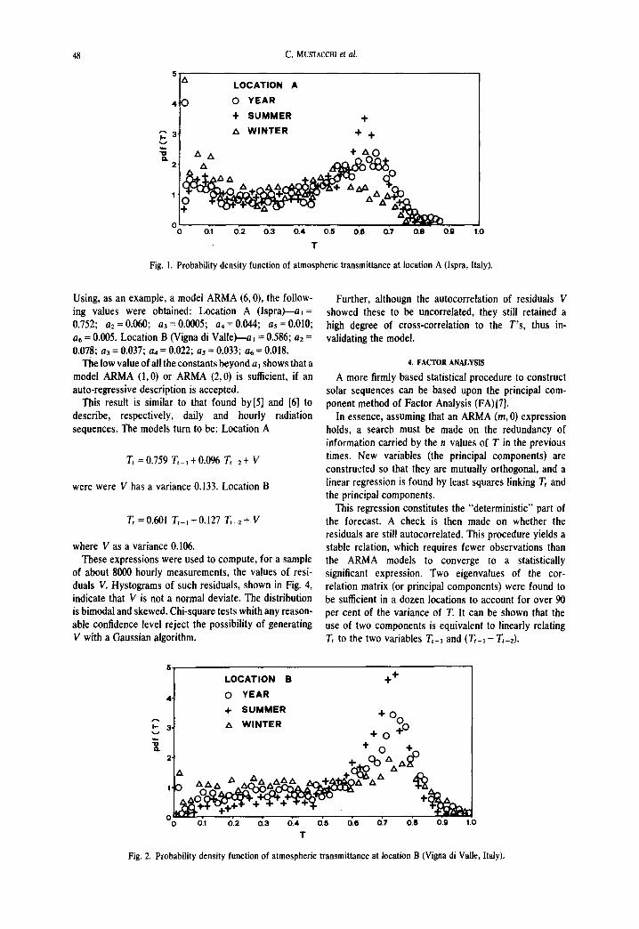
Fig. 3. Autocorrelation function of atmospheric transmittance, process, where a transition function is given, p(a, b) such that if T, = a, the probability of having 1",+, = b is

The simulations conducted with this type of model p(a, b). The transition probability is such that it depends exhibit better statistical properties, as compared with the only on the present state (a) and not upon the more ARMA models, but both models suffer from T's with a distant past. normal probability distribution function. As shown in the The simplest form of function p(a, b) is that of a Appendix, this difficulty is unavoidable, with any ARMA transition matrix, with elements Pab giving the prob- and FA model. Since the pdrs of Figs. 1 and 2 are very ability of changing from state a to state b in 1 hr. Such far from being normal, other approaches must be sought, matrices were constructed for the twelve sites examined

by building up the two-dimensional hystogram obtained from the transitions of several thousand contiguous

O couples of hourly observations of T. A graininess of these matrices compatible with the

A LOCATION A precision of pyranometric measurements turned out to 0 LOCATION B require 25x25 matrices, i.e. the range of T from 0 to 1

zxzx was split into intervals of width 0.04. s. " Simulations are conducted by selecting row a, cor-

,, responding to T,, and generating a random number R with a rectangular distribution in the range (0, 1). Ele-

4. ~A 0 ments Pa,, Pa2, Pa3... Pab are added until their sum is

zx greater than R. State b is then assigned to T,+~. 3 -

"g " 0 ~ The simulations thus conducted led, as shown in Fig. 5 zx 2. 0 ~ for Ispra, to a very good reconstruction of the dis-

ax tributions of Figs. ! and 2 of all the main statistically ~ important features of radiation sequences. In fact, a fast

1 ~ check on the quality of the transition matrix can exploit the fact that by raising this matrix to a high power

0 , , -0.6 -0.4 -0.2 0.0 0.2 0'.4 0~6 (typically 200), a new matrix is obtained with all its rows

v equal. The elements of the rows reproduce the ordinates Fig. 4. Probability density function of ARMA (2, 0) residuals, of the probability density function of T, i.e. Figs. l and 2.

"U

2~+

1 0

0

O ARMA (2,o)

"1" MARKOV MATRIX

+ +

o o O ° ° ° O o t . .+ + o + o

+ + o + o 4. + + +

o ~ + + o

dt o'.2 o.a 6.4 6.s de T

+

+ O

o'.7 de o.o I.o

Fig. 5. Probability density function of atmospheric transmittance simulated by means of an ARMA (2, 0) and a Markov transition technique (Location A).

5o

This model was found so consistently satisfactory that a generalized computer procedure was written to analize hourly data, build the transition matrix and simulate the hourly radiation.

Corrections of collector tilt use the Liu and Jordan[8], Orgill and Hollands[9] or the LASL methods[10] and results exhibit discrepancies of 2-3 per cent at most.

6. TRANSMITTANCE TRANSmON TENSOR

A step further in the direction of using a combined ARMA (n, 0) and a transition matrix approach is that of generalizing the latter description by constructing a transition tensor of order n. Such a tensor has n - l dimensions corresponding to the values of T in n - I successive times.

The elements along the nth dimension yield a value for the probability of having a given transition at the next time step. Thus, a model T/T(3) would use a third-order tensor which has elements p~k measuring the probability that if T, =j at present and Tt-~ = i l hr ago, then, the probability of having T,+~ = k I hr from now is given by pijk.

This approach was experimented with a third-order tensor obtained by analyzing several thousand triplets of transmittances at 1 hr intervals. The simulations derived from this model were but a slight improvement as com- pared with the Markov approach. The statistical significance of the tensor element decreased for lack of a sufficiently extended sample. It was therefore felt that such sophistication was not justified.

7. GAUSSIAN MAPPING

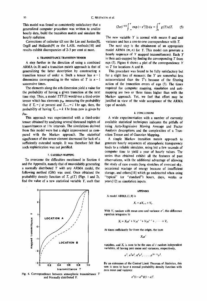
To overcome the difficulties mentioned in Section 4 and the Appendix, namely that of unavoidably generating a normally distributed T with any ARMA model, the following method (GM) was used. Once obtained the probability density function of T, g(T) (Figs. 1 and 2), find the value of a new statistical variable Y, such that

C. MUSTACCHI et al.

f: (2~r)- '~ exp ( - x2/2) dx = g(T) dr. (5)

The new variable Y is normal with means 0 and unit variance and has a one-to-one correspondence with T.

The next step is the obtainment of an appropriate model ARMA (m, n) for Y. This model can generate a hourly sequence of Y mapped transmittances). Each Y is then anti-mapped by finding the corresponding T from eqn (5). Figure 6 shows a plot of the correspondence Y vs T for locations A and B.

This procedure was found to be fully satisfactory but for a slight loss of memory: the Y are somewhat less autocorrelated than the T's because of the filtering action of the truncation errors of eqn (5). The times required for computer mapping, simulation and anti- mapping are two or three times higher than with the Markov approach. Yet, we feel that effort may be justified in view of the wide acceptance of the ARMA type of models.

8. CONCLUSIONS

A wide experimentation with a number of currently available statistical techniques indicates the pitfalls of using Auto-Regressive Moving Average and Factor Analysis descriptions and the complexities of a Tran- sition Tensor and of Gaussian Mapping.

A simple Markov transition matrix approach to generate hourly sequences of atmospheric transparency leads to a reliable simulator, using but a few seconds of computer time to yield a year of hourly values. The series thus obtained exhibit all the features of past observations, with the additional advantage of allowing the study of rare events (long stretches of overcast sky, occasional wastage of energy because of insufficient storage, and others [11] which go undetected when using "typical" (or "standard") hours, days, weeks or years [12] as simulation inputs.

3 / / 2,

>" I. / /I/ c °~ L O C A T I ~ / / / / I

.. i t , . / / / /

.=- O- E

"O -1. O e~e' / / / / / LOCATION B

-2- / /

-3 0 0:2 0.4 0:6 0:8 1.0 t ransmi t tance T

Fig. 6. Correspondence between atmospheric transmittance T and Normally distributed Y.

APPENDIX

A model ARMA (1,0) is

X, = aX,_, + V,.

With Vt random with mean zero and variance 02, this difference equation integrates to

Xt = Xo at + V,at - ' + Vzat-2+. . . . ' + Vt.

At times sufficiently far from the origin, the term

Xoa t

vanishes, and X, is seen to be the sum of t random independent variables, all having zero mean and variances, respectively,

0. -2, a20 -2, a40. 2, . . . . . ,d 2(t-I)0. 2.

By an extension of the Central Limit Theorem of Statistics, this sum is seen to have a normal probability density function with zero mean and variance

0.2(1 - a2')/(l - a) 2.

Stochastic simulation of hourly global radiation sequences 51

The same result applies to any ARMA (re, n) namely it will generate normal XI whatever is the shape of the pdf assigned to V.

It may be pointed out, however, that the theoretical possibility exists of constructing stationary sequences of variables with a specified marginal distribution (DARMA models)J13]. The rele- vant applications are currently under study.

REFERENCES

1. G. E. P. Box and G. M. Jenkins, Time Series Analysis-- Forecasting and Control. Holden-Day, San Francisco (1970),

2. A. Papoulis, Probability, Random Variables and Stochastic Processes. McGraw-Hill, New York (1965).

3. R. Dogniaux and M. Lemoine, Programme de calcul des 6clairements solaires 6nerg6tiques et lumineux de surfaces orient6es et inclin6es, lnstitut Mit#orologique de Belgique, Sdrie C No. 14 (1976).

4. K. Y. Kondratyev and M. P. Fedorova, Radiation regime of inclined surfaces. Proc. UNESCO-WMO Symp. on Solar Energy, WMO no. 477, Geneva (1977).

5. B. J. Brinkworth, Autocorrelation and stochastic modelling of insolation sequences. Solar Energy 19, 343 (1977).

6. T. N. Goh and K. J. Tan, Stochastic modelling and forecas- ting of solar radiation data. Solar Energy 19, 755 (1977).

7. H. H. Harman, Factor analysis, in Mathematical Methods for Digital Computers (Edited by A. Ralston and H. S. Will). Wiley, New York (1960).

8. B. Y. H. Liu and R. C. Jordan, The interrelationship and characteristic distribution of direct, diffuse and total solar radiation. Solar Energy 4, 3 (1960).

9. J. F. Orgill and K. G. T. Hollands, Correlation equation for hourly diffuse radiation on a horizontal surface. Solar Energy 19, 357 (1977).

10. International Energy Agency, Solar Heating and Cooling Program, Task 1, Prov. Rep. (Edited by O. Jergensen) (May 1978).

11. Joshua 10:13. 12. W. R. Petrie and M. McClintock, Determining typical wea-

ther for use in solar energy simulation. Solar Energy 21, 55 (1978).

13. P. A. Jacobs and P. A. Lewis, Discrete time series generated by mixtures. I: correlational and runs properties. J. Roy. Stat. Soc. B 40, 94 (1978).

Resumen~La simulaci6n aleatoria de la radiaci6n global horaria mediante las t6cnicas autoregresivas a media movil y del analisis factorial no describe las propriedades estadfsticas de Ins series temporarias. Un modelo de Markov a matriz de transici6n que actfia sobre ia transmici6n atmosf6rica permite una simulaci6n simple peru eficaz. Dos nuevos modelos sofisticados, o sea: el tensor de transici6n y el mapa Gausiano, son t6cnicas no justificadas a este fin.

Resum6--La simulation al~atoire du rayonnement global horaire moyennant les techniques auto-regressives moyenne mobile et de l'analyse factorielle ne d6crit pas les caract~res statistiques des s~ries temporelles. Un mod~le de Markov ~ matrice de transition qui agit sur la transmittance atmosph~rique permet une simulation simple mais efficace. Deux nouveaux mod~les, ~ savoir: ie tenseur de transition des transmissions et le mappag¢ Gaussien ne sont pas justifi6s darts ce contexte.