Stochastic Similarity For Validating Human Control ... AND XU: STOCHASTIC SIMILARITY FOR VALIDATING HUMAN CONTROL STRATEGY MODELS 439 Fig. 2. A 5-state HMM, with 16 observable symbols

IEEE TRANSACTIONS ON ROBOTICS AND AUTOMATION, VOL. 14, NO. 3, JUNE 1998 437

Stochastic Similarity for ValidatingHuman Control Strategy Models

Michael C. Nechyba,Student Member, IEEE,and Yangsheng Xu,Senior Member, IEEE

Abstract—Modeling dynamic human control strategy (HCS),or human skill in response to real-time sensing is becomingan increasingly popular paradigm in many different researchareas, such as intelligent vehicle systems, virtual reality, andspace robotics. Such models are often learned from experimentaldata, and as such can be characterized despite the lack of agood physical model. Unfortunately, learned models presentlyoffer few, if any, guarantees in terms of model fidelity to thetraining data. This is especially true for dynamic reaction skills,where errors can feed back on themselves to generate stateand command trajectories uncharacteristic of the source process.Thus, we propose a stochastic similarity measure—based onhidden Markov model (HMM) analysis—capable of comparingand contrasting stochastic, dynamic, multidimensional trajec-tories. This similarity measure is the first step in validatinga learned model’s fidelity to its training data by comparingthe model’s dynamic trajectories in the feedback loop to thehuman’s dynamic trajectories. In this paper, we first derive anddemonstrate properties of the similarity measure for stochasticsystems. We then apply the similarity measure to real-timehuman driving data by comparing different control strategiesamong different individuals. We show that the proposed similaritymeasure out performs the more traditional Bayes classifier incorrectly grouping driving data from the same individual. Finally,we illustrate how the similarity measure can be used in thevalidation of models which are learned from experimental data,and how we can connect model validation and model learning toiteratively improve our models of human control strategy.

Index Terms— Hidden Markov models, human modeling,model validation, neural networks, similarity measure.

I. INTRODUCTION

M ODELS of human skill, or human control strategy,which accurately emulate dynamic human behavior,

have far reaching potential in areas ranging from robotics tovirtual reality to the intelligent vehicle highway project. Signif-icant challenges arise in the modeling of human skill, however.Defying analytic representation, little if anything is knownabout the structure, order, or granularity of an individual’shuman controller. Human control strategy is both dynamicas well as stochastic in nature. In addition, the complexmapping from sensory inputs to control action outputs inherentin human control strategy can be highly nonlinear for giventasks. Therefore, developing an accurate and useful modelfor this type of dynamic phenomenon is frustrated by a poor

Manuscript received June 6, 1996; revised January 15, 1998. This work wassupported in part by a DOE doctoral fellowship. This paper was recommendedfor publication by Associate Editors F. Cervantes and B. Hannaford uponevaluation of the reviewers’ comments.

The authors are with The Robotics Institute, Carnegie Mellon University,Pittsburgh, PA 15213 USA.

Publisher Item Identifier S 1042-296X(98)02920-6.

understanding of the underlying basis for that phenomenon.Consequently, modeling by observation, rather than physicalderivation, is becoming an increasingly popular paradigm forcharacterizing a wide range of complex processes, includinghuman control strategy (HCS). This type of modeling is saidto constitute learning, since the model is not derived fromapriori laws of nature, but rather from observed instances ofexperimental data, known collectively as the training set.

The main strength of modeling by learning, is that noexplicit physical model is required; this also represents itsbiggest weakness, however. On the one hand, we are notrestricted by the limitations of current scientific knowledge,and are able to model HCS for which we have not yetdeveloped adequate biological or psychological understanding.On the other hand, the lack of scientific justification detractsfrom the confidence that we can show in these learned models.This is especially true when the unmodeled process is

1) dynamic;2) stochastic in nature, as is the case for human control

strategy.For a dynamic process, model errors can feed back on them-selves to produce trajectories which are not characteristic ofthe source process or are even potentially unstable. For astochastic process, a static error criterion (such as root meansquare (RMS) error), based on the difference between thetraining data and predicted model outputs may be inadequateand inappropriate to gauge the fidelity of a learned modelto the source process. Yet, most learning approaches today,including the cascade learning algorithm, utilize some staticerror measure as a test of convergence for the learningalgorithm. While this measure is very useful during training,it offers no guarantees, theoretical or otherwise, about thedynamic behavior of the resulting learned model.

For a simple illustration of this problem, consider thefollowing example. Suppose that we wish to learn a dy-namic process represented by the following simple differenceequation:

(1)

where represent the output and input of the system,respectively, at time step The input–output training data inTable I is provided.

Note that (1) is asymptotically stable. Now, suppose, forexample, that we train simple neural networks to learn threedifferent approximations of the system in (1)

(2)

(3)

(4)

1042–296X/98$10.00 1998 IEEE

438 IEEE TRANSACTIONS ON ROBOTICS AND AUTOMATION, VOL. 14, NO. 3, JUNE 1998

TABLE ISAMPLE INPUT–OUTPUT TRAINING DATA

Fig. 1. The three models result in dramatically different (even unstable)trajectories.

The three models all have the same RMS error for thetraining set in Table I. Nevertheless, the dynamic trajectoriesfor the three models differ significantly. For example, considerthe input

(5)

The resulting output for the system as well as the threemodels is shown in Fig. 1. Model #2 approximates the systemin (1) well; model #3 remains stable, but approximates thesystem with significantly poorer accuracy; finally, model #1diverges into an unstable trajectory.

The difference in the three models is the distribution ofthe error over the training set. Thus, a static error measure,such as RMS error, does not provide sufficiently satisfactorymodel validation for a dynamic process. Furthermore, forstochastic systems, one cannot expect equivalent trajectoriesfor the process and the learned model, given the same initialconditions. Thus, we require a stochastic similarity measure,with sufficient representational power and flexibility to com-pare multidimensional, stochastic trajectories. In this paper, wedevelop such a similarity measure, based on hidden Markovmodel (HMM) analysis, as a first step in validating models ofdynamic human control strategy.

This paper is organized into three parts.

1) First, using HMM’s, we derive a stochastic similaritymeasure capable of comparing arbitrary multidimen-

sional, stochastic trajectories. This measure makes noapriori assumptions about the statistical distribution of theunderlying data to be compared. We demonstrate certainproperties of the proposed similarity measure throughboth mathematical proof and simulation of known sto-chastic systems.

2) Second, we evaluate the similarity measure on humancontrol data, by comparing driving strategies amongdifferent individuals. We show that the proposed simi-larity measure outperforms the more traditional Bayesclassifier in correctly grouping driving data from thesame individual.

3) Finally, we illustrate how the similarity measure canbe used in the validation of models which are learnedfrom experimental data, and how we can connect modelvalidation and model learning to iteratively improve ourmodels of human control strategy.

II. STOCHASTIC SIMILARITY

Similarity measures or metrics have been given considerableattention in computer vision [1]–[3], image database retrieval[4], and two-dimensional (2-D) or three-dimensional (3-D)shape analysis [5], [6]. These methods, however, generallyrely on the special properties of images, and are thereforenot appropriate for analyzing sequential trajectories. Otherwork has focussed on classifying temporal patterns usingstandard statistical techniques [7], wavelet analysis [8], neuralnetworks [9], [10], and HMM’s (see discussion below). Muchof this work, however, analyzes only short-time trajectoriesor patterns, and, in many cases, generates only a binaryclassification, rather than a continuously valued similarity mea-sure. Prior work has not addressed the problem of comparinglong, multidimensional, stochastic trajectories, especially ofhuman control data. Thus, we propose to evaluate stochasticsimilarity between two dynamic, multidimensional trajectoriesusing HMM analysis.

A. Hidden Markov Models

Rich in mathematical structure, HMM’s are trainable statis-tical models, with two appealing features:

1) no a priori assumptions are made about the statisticaldistribution of the data to be analyzed;

2) a high degree of sequential structure can be encoded bythe HMM’s.

As such, they have been applied for a variety of stochasticsignal processing. In speech recognition, where HMM’s havefound their widest application, human auditory signals areanalyzed as speech patterns [11], [12]. Transient sonar signalsare classified with HMM’s for ocean surveillance in [13].Radonset al. [14] analyze 30-electrode neuronal spike activityin a monkey’s visual cortex with HMM’s. Hannaford and Lee[15] classify task structure in teleoperation based on HMM’s.In [16] and [17], HMM’s are used to characterize sequentialimages of human actions. Finally, Yang and Xu apply HMM’sto open-loop action skill learning [18] and human gesturerecognition [19].

NECHYBA AND XU: STOCHASTIC SIMILARITY FOR VALIDATING HUMAN CONTROL STRATEGY MODELS 439

Fig. 2. A 5-state HMM, with 16 observable symbols in each state.

A HMM consists of a set of states, interconnectedthrough probabilistic transitions; each of these states has someoutput probability distribution associated with it. Althoughalgorithms exist for training HMM’s with both discrete andcontinuous output probability distributions, and although mostapplications of HMM’s deal with real-valued signals, discreteHMM’s are preferred to continuous HMM’s in practice, due totheir relative computational simplicity and lesser sensitivity toinitial random parameter settings [20]. In Section II-D below,we describe how we use discrete HMM’s for analysis ofreal-valued signals by converting the data to discrete symbolsthrough preprocessing and vector quantization. Thus, a discreteHMM is completely defined by the following triplet [12]:

(6)

where is the probabilistic state transition matrix,is the output probability matrix with discrete

output symbols and is the -length initialstate probability distribution vector for the HMM. Fig. 2,for example, represents a 5-state HMM, where each stateemits one of 16 discrete symbols, based on some probabilitydistribution.

For an observation sequence of discrete symbols, wecan locally maximize (i.e. the probability of themodel given the observation sequence using theBaum–Welch Expectation-Maximization (EM) algorithm [12],[21]. Throughout this paper, we initialize the Baum–Welchalgorithm by setting the HMM parameters to random, nonzerovalues, subject of course to the necessary probabilisticconstraints. We can also evaluate (i.e., the probabilitythat a given observation sequenceis generated from themodel ).

Finally, two HMM’s and are defined to be equivalent

(7)

Note that and need not be identical to be equivalent.The following two HMM’s are, for example, equivalent:

(8)

B. Similarity Measure

Below, we derive a stochastic similarity measure, basedon discrete-output HMM’s. Let denote adistinct observation sequence of discrete symbols with length

Also, let denote

Fig. 3. Four normalized probability values make up the similarity measure.

a discrete HMM locally optimized using the Baum–Welchalgorithm to maximize Similarly, letdenote the probability of the observation sequencegiventhe model and let

(9)

denote the probability of the observation sequencegiventhe model normalized with respect to In practice, wecalculate as

(10)

to avoid problems of numerical underflow for long observationsequences.

Using the definition in (9), Fig. 3 illustrates our overallapproach to evaluating similarity between two observationsequences. Each observation sequence is first used to train acorresponding HMM; this allows us to evaluate andFurthermore, we subsequently cross-evaluate each observationsequence on the other HMM (i.e., toarrive at and Given, these four normalized proba-bility values, we now define the following similarity measurebetween and :1

(11)

This measure takes the ratio of the cross probabilities overthe training probabilities, and normalizes for the multiplicationof the two probability values in the numerator and denominatorby taking the square root.

Because and are necessarily trained on finite-lengthtraining sequences, rare events—either rare state transitionsor rare observations—may not be recorded in either or both

and forcing corresponding parameters in the HMM’sto converge to zero during training. This can causeand to degenerate to zero, even when and are,in fact, almost identical. For example, suppose andare identical observation sequences. Then, willevaluate to one. Replacing just one observation inwithan observable not present in however, will forceand hence to zero, even though the one rogueobservation could simply be a measurement or recording error.To overcome this singularity problem and to account for

1In [22], we proposed a different similarity measure for which properties #1,#2, and #3 do not hold. Thus, the previous similarity measure gives potentiallyinconsistent and misleading results for certain data. The similarity measure in(11) corrects these problems.


the possibility of rare, but unobserved events, we follow thecommon practice of replacing nonzero elements in the trainedHMM’s by some and renormalizing the model to fitprobabilistic constraints [12]. Therefore, we calculate thenot on itself, but rather a smoothed version ofwhere zero elements in the matrices are replacedby 0.0001. This value of is chosen as it redistributesless than 0.1% of the probability mass in the state transitionmatrix and less than 0.5% of the probability mass in theoutput probability matrix

C. Properties

For now, assume that is a global (rather than just alocal) maximum. Then

(12)

and

(13)

The lower bound for in (12) is realized for single-statediscrete HMM’s, and a uniform distribution of symbols inFrom (11)–(13), we can establish the following properties for

:

Property by definition

(14)

Property (15)

Property

(16)

As we have noted before, the Baum-Welch algorithm guar-antees only that is a local maximum. In practice, this is nota significant concern, however, as the Baum–Welch algorithmconverges to near-optimal solutions, when the algorithm isinitialized with random model parameters [12], [20]. We canverify this near-optimal convergence property experimentally.First, for a given model we generate a long observationsequence Next, we train a second HMM with initialrandom model parameters on Finally, we evaluate thenormalized probability values and Ifis near-optimal or optimal for sequence then

(17)

provided that is sufficiently long. We have used both thisprocedure as well as multiple training runs from differentrandom initial parameter settings to verify the near-optimalconvergence properties of the Baum–Welch algorithm for thetype of data (i.e., human control data) studied in this paper.

Below, we illustrate the behavior of the similarity measurefor some simple HMM’s. First, for single-state HMM’s, thesimilarity measure reduces to

(18)

which reaches a maximum when or simply,and that maximum is equal to one. Fig. 4 shows

Fig. 4. Similarity measure for two binomial distributions. Lighter colorsindicate higher similarity.

a contour plot for

(19)

whereSecond, we give an example of how the proposed similarity

measure changes, not as a function of different symbol distri-butions, but rather as a function of varying HMM structure.Consider the following HMM:

(20)

and corresponding observation sequences, stochasticallygenerated from model For all willhave an equivalent aggregate distribution of symbols 0 and1—namely 1/2 and 1/2. As increases, however, willbecome increasingly structured. For example

equivalent to unbiased coin toss (21)

(22)

Fig. 5 graphs as a contour plot forwhere each observation sequence of lengthis generated stochastically from the corresponding

HMM 2 Greatest similarity is indicated forwhile greatest dissimilarity occurs for and

In some cases, it may be more convenient to representthe similarity between two trajectories through a distancemeasure rather than a similarity measure. Given

2This procedure only approximates our similarity measure definition, since�(�) is only optimal forO(�) asT !1:


Fig. 5. The similarity measure changes predictably as a function of HMMstructure.

the similarity measure such a measure is easilyderived. Let

(23)

such that

(24)

(25)

if a or b

(26)

The distance measure between two observationsequences defined in (23) is closely related to the dual notionof distance between two HMM’s, as proposed in [23].

Let denote a random observation sequence of lengthgenerated by the HMM and let

(27)

Then, [23] defines the following distance measure betweentwo HMM’s, and

(28)

Unlike the observation sequences the sequences arenot unique, since they are stochastically generated fromHence, is uniquely determined only in the limit as

Likewise for the HMM’s and arenot unique, since and are in general guaranteed to beonly local, not global maxima. Hence, is uniquelydetermined only when and represent global maxima.

While in general, and are not equiv-alent, the discussion above suggests sufficient conditions for

(a)

(b)

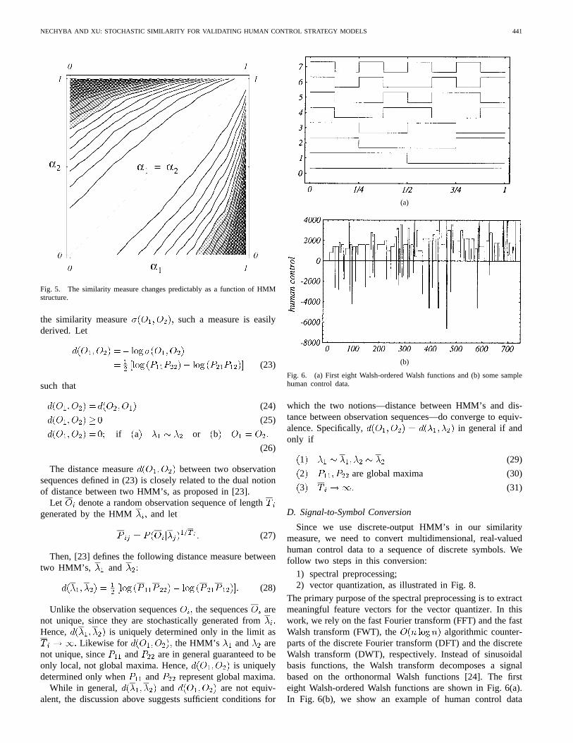
Fig. 6. (a) First eight Walsh-ordered Walsh functions and (b) some samplehuman control data.

which the two notions—distance between HMM’s and dis-tance between observation sequences—do converge to equiv-alence. Specifically, in general if andonly if

1 (29)

2 are global maxima (30)

3 (31)

D. Signal-to-Symbol Conversion

Since we use discrete-output HMM’s in our similaritymeasure, we need to convert multidimensional, real-valuedhuman control data to a sequence of discrete symbols. Wefollow two steps in this conversion:

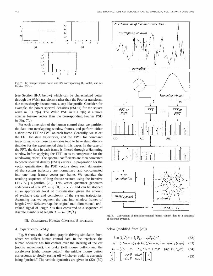
1) spectral preprocessing;2) vector quantization, as illustrated in Fig. 8.

The primary purpose of the spectral preprocessing is to extractmeaningful feature vectors for the vector quantizer. In thiswork, we rely on the fast Fourier transform (FFT) and the fastWalsh transform (FWT), the algorithmic counter-parts of the discrete Fourier transform (DFT) and the discreteWalsh transform (DWT), respectively. Instead of sinusoidalbasis functions, the Walsh transform decomposes a signalbased on the orthonormal Walsh functions [24]. The firsteight Walsh-ordered Walsh functions are shown in Fig. 6(a).In Fig. 6(b), we show an example of human control data


(a) (b)

(c)

Fig. 7. (a) Sample square wave and it’s corresponding (b) Walsh, and (c)Fourier PSD’s.

(see Section III-A below) which can be characterized betterthrough the Walsh transform, rather than the Fourier transform,due to its sharply discontinuous, step-like profile. Consider, forexample, the power spectral densities (PSD’s) for the squarewave in Fig. 7(a). The Walsh PSD in Fig. 7(b) is a moreconcise feature vector than the corresponding Fourier PSDin Fig. 7(c).

For each dimension of the human control data, we partitionthe data into overlapping window frames, and perform eithera short-time FFT or FWT on each frame. Generally, we selectthe FFT for state trajectories, and the FWT for commandtrajectories, since these trajectories tend to have sharp discon-tinuities for the experimental data in this paper. In the case ofthe FFT, the data in each frame is filtered through a Hammingwindow before applying the FFT, so as to compensate for thewindowing effect. The spectral coefficients are then convertedto power spectral density (PSD) vectors. In preparation for thevector quantization, the PSD vectors along each dimensionof the system trajectory are normalized and concatenatedinto one long feature vector per frame. We quantize theresulting sequence of long feature vectors using the iterativeLBG VQ algorithm [25]. This vector quantizer generatescodebooks of size and can be stoppedat an appropriate level of discretization given the amountof available data and complexity of the system trajectories.Assuming that we segment the data into window frames oflength with 50% overlap, the original multidimensional, real-valued signal of length is thus converted to a sequence ofdiscrete symbols of length

III. COMPARING HUMAN CONTROL STRATEGIES

A. Experimental Set-Up

Fig. 9 shows the real-time graphic driving simulator, fromwhich we collect human control data. In the interface, thehuman operator has full control over the steering of the car(mouse movement), the brake (left mouse button) and theaccelerator (right mouse button); the middle mouse buttoncorresponds to slowly easing off whichever pedal is currentlybeing “pushed.” The vehicle dynamics are given in (32)–(50)

Fig. 8. Conversion of multidimensional human control data to a sequenceof discrete symbols.

below (modified from [26])

(32)

(33)

(34)

(35)


where

angular velocity of the car (36)

longitudinal velocity of the car (37)

(38)

(39)

(40)

rear tire slip angle (41)

(42)

body-relative lateral axis

body-relative longitudinal axis (43)

cornering stiffness of frontrear tires

N/rad N/rad (44)

lumped coefficient of drag (air resistance)

m (45)

coefficient of friction

(46)

longitudinal force on rear tires

(47)

kg kg-m m

m m (48)

and the controls are given by

longitudinal force on front tires

(49)

rad steering angle rad (50)

Note that the separate brake and gas commands for thehuman are, in fact, the single variable, where the signindicates whether the brake or the gas is active [Fig. 6(b), forexample, illustrates one person’s profile for part of onerun]. The entire simulator is run at 50 Hz.

B. Similarity Results

For the first set of experiments, we ask five people:

1) Larry;2) Curly;3) Moe;4) Groucho;5) Harpo;

to practice driving in the simulator for a period of up to 15min to become accustomed to the simulator’s dynamics. Wethen record driving data for each person on three different,randomly generated 20 km roads, with only short breaks inbetween each run. Thus, we have a total of 15 runs.

Fig. 9. The driving simulator generates a perspective view of the road forthe user, who has independent control over steering, braking, and acceleration(gas).

Each road is described by a sequence of randomly generatedsegments of the form (straight-line segments), and(curves), connected in a manner that ensures continuous firstderivatives between segments. We also place the followingconstraints on individual segments:

m m

length of a straight- (51)

m m radius of curvature (52)

sweep angle of curve (53)

Therefore, each segment is one of the following:

1) straight line segment ( 0);2) left curve ( 0);3) right curve ( 0).

No segment may be followed by a segment of the same type;a curve is followed by a straight line segment with probability0.4, and an opposite curve segment with probability 0.6. Astraight line segment is followed by a left curve or right curvewith equal probability. Roads are defined to be 10 m wide(the car is 2 m wide), and the visible horizon is set to 100m. Fig. 10(a)–(c) show the three different roads used for theseexperiments.

For notational convenience, let

(54)

denote the run from person (i) on road Table II belowreports some aggregate statistics for each of the 15 runs.

Our goal here is to see

1) how well the similarity measure classifies each individ-ual’s runs across different roads;

2) how the classification performance of the proposed sim-ilarity measure compares with a more conventionalstatistical technique, namely the Bayes optimal classifier.


(a) (b) (c)

Fig. 10. (a) Road 1, (b) road 2, and (c) road 3.

The system trajectory for the driving task is defined by thethree state variables and the two control variables

For all the similarity results below (unless otherwisenoted), we choose the following spectral preprocessing:

- - - - - (55)

where F- denotes the k-point FFT, and W-denotes the k-point Walsh transform, with 50% overlappingwindow frames. Note that the PSD vector for a k-pointtransform has length thus, the feature vector to bequantized is of length 45. Also, note that we choose the Walshtransform for the two control variables since the user’scontrol is generally discontinuous and step-like in profile [asshown in Fig. 6(b) above]. When vector quantized, the featurevectors generated by the Walsh transform exhibit significantlyreduced distortion as compared to the Fourier-transformedfeature vectors for the two control variables.

From the preprocessed data, we build three vector code-books each with 128 levels, and corre-sponding to data from For theseexperiments, the number of levels in the VQ codebook isprimarily constrained by the amount of available data to trainthe HMM’s, since we want

length of each observation sequence

model parameters (56)

and the number of model parameters increases with the numberof levels in the VQ codebook. Now define

(57)

as the observation sequence of discrete symbols vector quan-tized from the preprocessed feature vectors of run usingthe codebook We can view the observation sequences

as control strategy data which we have already collected,processed, and modeled, without any information about theother data ( ). Thus, each sequence representsa class for individual . On the other hand, we can view theobservation sequences as new control data, whichwe wish to classify, using our similarity measure, as belonging

TABLE IIAGGREGATE STATISTICS FOR HUMAN DRIVING DATA

to one of the five individuals represented by the classes.For a given application, there will generally be known datafrom which we define our classes (represented here by thesequences ), and unknown data which we require to beclassified into one of the defined classes (represented hereby the sequences ). In this context, it would bequite burdensome to recalculate the vector codebook each timewe wish to classify a new control trajectory. Having separatecodebooks (for only the known data) eliminates the need forthis codebook recalculation.

Tables III–V classify each of the based onfor 1, 2, and 3, respectively, for eight-

state HMM’s. Note that the maximum value in each row ishighlighted. We consider classified correctly ifand only if

(58)

In other words, we expect that two runs from the sameindividual (but on different roads) will yield a higher similaritymeasure than two runs from two different individuals. Fromthe tables, we observe that the similarity measure correctlyclassifies all 30 comparisons, by assigning the highest similar-ity between runs from the same individual, and significantlylower similarity between runs from two different individuals.

Now we compare these classification results with the Bayesoptimal classifier. Define class as

(59)


TABLE III(a) SIMILARITY MEASURE CLASSIFICATION AND (b)

BAYES OPTIMAL CLASSIFICATION FOR ROAD #1 DATA

(a)

(b)

where is the mean vector for and is the covariancematrix for run For each road we have five classes,one corresponding to each individual. Each data point

in is now classified into classaccording to the Bayes decision rule [7]

(60)

where

(61)

(62)

In Tables III–V we report the percentage of data points inwhich are classified in class for 1,

2, and 3, respectively. We consider to be classifiedcorrectly when a plurality of the data from falls into class

and observe, from the tables, that the Bayes optimal

TABLE IV(a) SIMILARITY MEASURE CLASSIFICATION AND (b)


(a)

(b)

classifier misclassifies seven out 30 (23%) of the runs. Theperformance of the similarity measure (0% error) thereforecompares quite favorably.

Next, we present results for task-based classification. Weselect from each run all the left-turn maneuvers, and all theright-turn maneuvers. We get two resulting sets of maneuversfor each person

(63)

where corresponds to all the left-turn maneuvers for personi, and corresponds to all the right-turn maneuvers for personi. We then split each of these sets into two—one to train a VQcodebook (or calculate the Bayesian statistics), the other todetermine a similarity value (or the Bayesian classification).Tables VI and VII report the results for the similarity measure(seven-state HMM’s), and the Bayesian classification. Noteagain that the similarity measure classifies all ten sets (fiveleft-turn, five right-turn) correctly, while, the Bayes classifiermisclassifies three out of ten (30%).


TABLE V(a) SIMILARITY MEASURE CLASSIFICATION AND (b)


(a)

(b)

Finally, we present classification results for data which ismore difficult to classify. Moe is asked to drive over the sameroad on two different days, two times each day, generatingfour runs (#1, #2, #3, #4). Because the runs are recorded on thesame road, Moe is able to improve his skill relatively quickly.As recorded in Table VIII, his average speed improves from65.9–71.9 mi/h. from run #1–#4. We take two additional datasets, one from Larry and one from Curly, over the same road.These data sets have similar aggregate statistics compared toat least some of Moe’s runs.

Now we generate a 64-level VQ codebook with data fromLarry’s and Moe’s fourth run, and another 64-level VQcodebook with data from Curly’s and Moe’s fourth run. Wealso generate corresponding classes for the Bayes-classifiercomparison. We now classify each of Moe’s first three runsas either similar to Larry or Moe #4, or as either similar toCurly or Moe #4.

Table IX shows the classification results based on the sim-ilarity measure and Bayesian statistics. We observe that thesimilarity measure misclassifies one out of six (17%), while

TABLE VI(a) SIMILARITY MEASURE CLASSIFICATION AND (b)BAYES OPTIMAL CLASSIFICATION FOR LEFT TURNS

(a)

(b)

TABLE VII(a) SIMILARITY MEASURE CLASSIFICATION AND (b)BAYES OPTIMAL CLASSIFICATION FOR RIGHT TURNS

(a)

(b)

the Bayes classifier misclassifies five out of six (83%), somequite badly.

C. Discussion

Here, we discuss two issues which have not yet beenaddressed in the above results. First, we demonstrate whythe Bayes classifier fails in some cases, where the similaritymeasure succeeds. Fig. 11(a) plots the distribution (overand

of Curly’s data (Table VIII), and the Gaussian approxi-


(a) (b) (c)

(d) (e) (f)

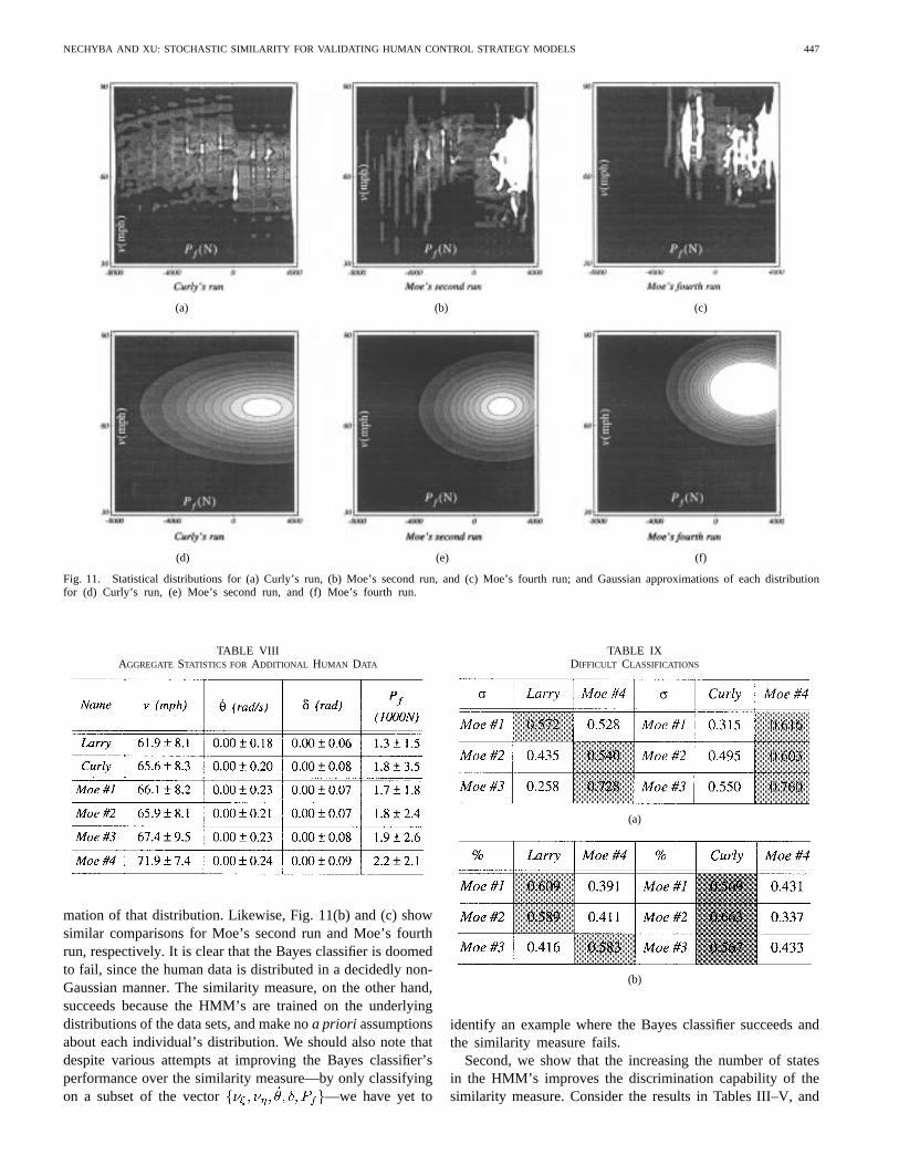
Fig. 11. Statistical distributions for (a) Curly’s run, (b) Moe’s second run, and (c) Moe’s fourth run; and Gaussian approximations of each distributionfor (d) Curly’s run, (e) Moe’s second run, and (f) Moe’s fourth run.

TABLE VIIIAGGREGATE STATISTICS FOR ADDITIONAL HUMAN DATA

mation of that distribution. Likewise, Fig. 11(b) and (c) showsimilar comparisons for Moe’s second run and Moe’s fourthrun, respectively. It is clear that the Bayes classifier is doomedto fail, since the human data is distributed in a decidedly non-Gaussian manner. The similarity measure, on the other hand,succeeds because the HMM’s are trained on the underlyingdistributions of the data sets, and make noa priori assumptionsabout each individual’s distribution. We should also note thatdespite various attempts at improving the Bayes classifier’sperformance over the similarity measure—by only classifyingon a subset of the vector —we have yet to

TABLE IXDIFFICULT CLASSIFICATIONS

(a)

(b)

identify an example where the Bayes classifier succeeds andthe similarity measure fails.

Second, we show that the increasing the number of statesin the HMM’s improves the discrimination capability of thesimilarity measure. Consider the results in Tables III–V, and


(a)

(b)

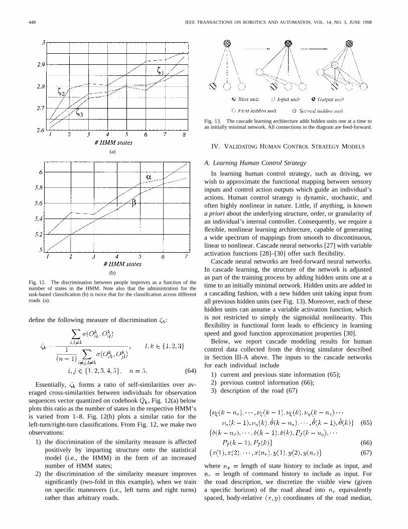
Fig. 12. The discrimination between people improves as a function of thenumber of states in the HMM. Note also that the administration for thetask-based classification (b) is twice that for the classification across differentroads (a).

define the following measure of discrimination:

(64)

Essentially, forms a ratio of self-similarities over av-eraged cross-similarities between individuals for observationsequences vector quantized on codebookFig. 12(a) belowplots this ratio as the number of states in the respective HMM’sis varied from 1–8. Fig. 12(b) plots a similar ratio for theleft-turn/right-turn classifications. From Fig. 12, we make twoobservations:

1) the discrimination of the similarity measure is affectedpositively by imparting structure onto the statisticalmodel (i.e., the HMM) in the form of an increasednumber of HMM states;

2) the discrimination of the similarity measure improvessignificantly (two-fold in this example), when we trainon specific maneuvers (i.e., left turns and right turns)rather than arbitrary roads.

Fig. 13. The cascade learning architecture adds hidden units one at a time toan initially minimal network. All connections in the diagram are feed-forward.

IV. V ALIDATING HUMAN CONTROL STRATEGY MODELS

A. Learning Human Control Strategy

In learning human control strategy, such as driving, wewish to approximate the functional mapping between sensoryinputs and control action outputs which guide an individual’sactions. Human control strategy is dynamic, stochastic, andoften highly nonlinear in nature. Little, if anything, is knowna priori about the underlying structure, order, or granularity ofan individual’s internal controller. Consequently, we require aflexible, nonlinear learning architecture, capable of generatinga wide spectrum of mappings from smooth to discontinuous,linear to nonlinear. Cascade neural networks [27] with variableactivation functions [28]–[30] offer such flexibility.

Cascade neural networks are feed-forward neural networks.In cascade learning, the structure of the network is adjustedas part of the training process by adding hidden units one at atime to an initially minimal network. Hidden units are added ina cascading fashion, with a new hidden unit taking input fromall previous hidden units (see Fig. 13). Moreover, each of thesehidden units can assume a variable activation function, whichis not restricted to simply the sigmoidal nonlinearity. Thisflexibility in functional form leads to efficiency in learningspeed and good function approximation properties [30].

Below, we report cascade modeling results for humancontrol data collected from the driving simulator describedin Section III-A above. The inputs to the cascade networksfor each individual include

1) current and previous state information (65);2) previous control information (66);3) description of the road (67)

(65)

(66)

(67)

where length of state history to include as input, andlength of command history to include as input. For

the road description, we discretize the visible view (givena specific horizon) of the road ahead into equivalentlyspaced, body-relative coordinates of the road median,


(a)

(b)

Fig. 14. (a) Oliver’s driving data and (b) Stan’s driving data. On the left ofeach figure, we show part of the source training data; on the right of eachfigure we show the corresponding model-generated data.

and provide that sequence of coordinates as input to thenetwork. Thus, for fixed and the total number ofinputs to the network will be

(68)

The outputs for the cascade network are, of course,(i.e., the steering and acceleration command

for the next time step).

B. Similarity Results

The left sides of Fig. 14(a) and (b) show part of the drivingdata collected from two individuals, Oliver and Stan. Note thatthe driving styles for the two individuals are quite differentfor the same road. The right sides of Fig. 14(a) and (b) showpart of the cascade model-generated command trajectories forOliver and Stan. Since Stan’s control strategy is relativelysimple, his control strategy model requires 30 hidden unitsand only the previous two states as input (i.e., 2).

TABLE XHUMAN-TO-MODEL SIMILARITY RESULTS

Oliver’s more complicated control strategy model, on the otherhand, requires 32 hidden units and relies on the previous tenstates ( 10) to stay on the road. We determine theseinput histories experimentally to achieve stable road followingfor each HCS model. For both models, we let 15.

Table X below summarizes the similarity results for thedata in Fig. 14. All preprocessing and vector quantization wasperformed in the same manner as in Section III-B.

C. Discussion and Future Work

The similarity results in Table X confirm two qualitativeassessments of the data in Fig. 14(a) and (b). First, we observethat the two driving styles are objectively quite different.This fact is reflected in the low similarity measures betweenone individual’s model and the other individual’s sourceand model-generated data. Second, Stan’s model is a betterreflection of his driving style, than Oliver’s model is of his, asreflected in the two respective similarity measures, 0.748 and0.349. This is indicative that Oliver’s sharply discontinuousdriving strategy is more difficult to learn by a single cascadenetwork than Stan’s calmer approach. Indeed, Oliver’s modelgenerates significant oscillatory behavior, of which Oliverhimself is not guilty.

Thus, the relatively low similarity measure between Oliverand Oliver’s model points to a problem in the model itself,including possible improper assumptions about the controllerorder, granularity and control delay of the actual HCS. As amatter of fact, the values for and for each modelwere arrived at in an essentiallyad hoc manner. To correctthis problem, we are at present working on an algorithm toimprove a model’s input representation based on the similaritymeasure. We propose combining the similarity measure withsimultaneously perturbed stochastic approximation (SPSA)[31] to select the best model input representation.

In general, a given control strategy can be approximated by

(69)

where is some arbitrary unknown function, is avector of control outputs, is a vector of sensory inputs(including both state and environment variables) at time step

indicates the controller resolution or granularity, and


Fig. 15. Overall approach to model refinement using the similarity measure.

indicates the control delay. The order of the dynamic systemis given by the constants and In order to select the bestinput representation for the HCS model, we need to optimizethe parameter vector

(70)

for some given experimental data. Let, denote a trainedHCS model with input representation and let

denote the similarity measure for model Now, thebest input representation is defined in terms of the similaritymeasure such that

(71)

This optimization is difficult in principle since

1) we have no explicit gradient information

(72)

2) each measurement of is computationally expensive.

Thus, we resort to simultaneously perturbed stochastic approx-imation to perform the optimization. We propose to evaluatethe similarity measure for two values of in order to arriveat a new estimate for at iteration Fig. 15 illustrates theoverall loop, where is a vector of mutually independent,mean-zero random variables (e.g., symmetric Bernoulli dis-tributed), the sequence is independent and identicallydistributed, and the are positive scalar sequences.

V. CONCLUSION

Model validation is an important problem in the area ofmachine learning for dynamic systems, if learned modelsare to be exploited to their full potential. In this paper,

we have derived a stochastic similarity measure, based onHMM analysis, by which we can compare and contrast arbi-trary, multidimensional, stochastic trajectories. We have shownthat this method performs significantly better than traditionalstatistical techniques in classifying human control strategydata. Furthermore, we have shown that the similarity measureoffers a feasible means of validating a learned HCS model’sperformance to its training data. Finally, we have proposedan iterative algorithm, based on the similarity measure, whichallows us to refine a model’s input representation to improvemodel fidelity. Such an algorithm is of special relevance inlearning human control strategy, where little is knowna prioriabout the structure, order, or granularity of each individual’shuman controller.

ACKNOWLEDGMENT

The authors would like to thank the many people whopatiently “drove” through our driving simulator. Special thanksgo to O. Barkai, A. Gove, C. Lee, J. Murphy, and M. Ollisfor their patience as they navigated through some 50 mi ofsimulated road.

REFERENCES

[1] R. Basri and D. Weinshall, “Distance metric between 3-D models and 2-D images for recognition and classification,”IEEE Trans. Pattern Anal.Machine Intell., vol. 43, pp. 465–479, 1996.

[2] M. Boninsegna and M. Rossi, “Similarity measures in computer vision,”Pattern Recognit. Lett., vol. 15, no. 12, pp. 1255–1260, 1994.

[3] M. Werman and D. Weinshall, “Similarity and affine invariant distancesbetween 2-D point sets,”IEEE Trans. Pattern Anal. Machine Intell.,vol. 17, pp. 810–814, 1995.

[4] R. Jainet al., “Similarity measures for image databases,” inProc. IEEEInt. Conf. Fuzzy Syst., vol. 3, pp. 1247–1254, 1995.

[5] K. Y. Kupeev and H. J. Wolfson, “On shape similarity,” inProc. 12thIAPR Int. Conf. Pattern Recog., 1994, vol. 1, pp. 227–231.

[6] H. Y. Shum, M. Hebert, and K. Ikeuchi, “On 3-D shape similarity,”Tech. Rep. CMU-CS-95-212, Carnegie Mellon Univ., Pittsburgh, PA,1995.

[7] R. O. Duda and P. E. Hart,Pattern Classification and Scene Analysis.New York: Wiley, 1973.

[8] M. Sun, G. Burk, and R. J. Sclabassi, “Measurement of signal similarityusing the maxima of the wavelet transform,” inProc. IEEE Int. Conf.Acoustics, Speech, Signal Process, 1993, vol. 3, pp. 583–586.

[9] J. Hertz, A. Krogh, and R. G. Palmer,Introduction to the Theory ofNeural Computation. Redwood City, CA: Addison-Wesley, 1991.

[10] L. G. Sotelino, M. Saerens, and H. Bersini, “Classification of temporaltrajectories by continuous-time recurrent nets,”Neural Networks, vol.7, no. 5, pp. 767–776, 1994.

[11] X. D. Huang, Y. Ariki, and M. A. Jack,Hidden Markov Models forSpeech Recognition. Edinburg, U.K.: Edinburgh Univ. Press, 1990.

[12] L. R. Rabiner, “A tutorial on hidden Markov models and selectedapplications in speech recognition,”Proc. IEEE, vol. 77, pp. 257–286,1989.

[13] A. Kundu, G. C. Chen, and C. E. Persons, “Transient sonar signalclassification using hidden Markov models and neural nets,”IEEE J.Oceanic Eng., vol. 19, pp. 87–99, 1994.

[14] G. Radons, J. D. Becker, B. Dulfer, and J. Kruger, “Analysis, classi-fication and coding of multielectrode spike trains with hidden Markovmodels,”Biol. Cybern., vol. 71, no. 4, pp. 359–373, 1994.

[15] B. Hannaford and P. Lee, “Hidden Markov model analysis offorce/torque information in telemanipulation,”Int. J. Robot. Res., vol.10, no. 5, pp. 528–539, 1991.

[16] J. Yamato, S. Kurakake, A. Tomono, and K. Ishii, “Human actionrecognition using HMM with category separated vector quantization,”Trans. Inst. Electron., Inform. Comm. Eng. D-II, vol. J77D-II, no. 7, pp.1311–1318, 1994.

[17] J. Yamato, J. Ohya, and K. Ishii, “Recognizing human action in time-sequential images using hidden Markov models,”Trans. Inst. Electron.,Inform., Comm. Eng. D-II, vol. J76D-II, no. 12, pp. 2556–2563, 1993.


[18] J. Yang, Y. Xu, and C. S. Chen, “Hidden Markov model approach toskill learning and its application to telerobotics,”IEEE Trans. Robot.Automat., vol. 10, pp. 621–631, 1994.

[19] , “Human action learning via hidden Markov models,”IEEETrans. Syst., Man, Cybern A, vol. 27, pp. 34–44, Jan. 1997.

[20] L. R. Rabiner, B. H. Juang, S. E. Levinson, and M. M. Sondhi, “Someproperties of continuous hidden Markov model representations,”AT&TTech. J., vol. 64, no. 6, pp. 1211–1222, 1986.

[21] L. E. Baum, T. Petrie, G. Soules, and N. Weiss, “A maximizationtechnique occurring in the statistical analysis of probabilistic functionsof Markov chains,”Ann. Math. Stat., vol. 41, no. 1, pp. 164–171, 1970.

[22] M. C. Nechyba and Y. Xu, “On the fidelity of human skill models,” inProc. IEEE Int. Conf. Robot. Automat., 1996, vol. 3, pp. 2688–2693.

[23] B. H. Juang and L. R. Rabiner, “A probabilistic distance measure forhidden Markov models,”AT&T Tech. J., vol. 64, no. 2, pp. 391–408,1985.

[24] K. R. Rao and D. F. Elliott,Fast Transforms: Algorithms, Analyzes andApplications. New York: Academic, 1982.

[25] Y. Linde, A. Buzo, and R. M. Gray, “An algorithm for vector quantizerdesign,” IEEE Trans. Commun., vol. COM-28, pp. 84–95, 1980.

[26] H. Hatwal and E. C. Mikulcik, “Some inverse solutions to an automobilepath-tracking problem with input control of steering and brakes,”Veh.Syst. Dynam., vol. 15, pp. 61–71, 1986.

[27] S. E. Fahlman and C. Lebiere, “The cascade-correlation learning algo-rithm,” Tech. Rep. CMU-CS-90-100, Carnegie Mellon Univ., Pittsburgh,PA, 1990.

[28] M. C. Nechyba and Y. Xu, “Neural network approach to control systemidentification with variable activation functions,” inProc. IEEE Int.Symp. Intell. Contr., 1994, vol. 1, pp. 358–363.

[29] , “Human skill transfer: Neural networks as learners and teach-ers,” in Proc. IEEE Int. Conf. Intell. Robots Syst., vol. 3, pp. 314–319,1995.

[30] , “Toward human control strategy learning: Neural networkapproach with variable activation functions,” Tech. Rep. CMU-RI-TR-95-09, Carnegie Mellon Univ., Pittsburgh, PA, 1995.

[31] J. C. Spall, “Multivariate stochastic approximation using a simultaneousperturbation gradient approximation,”IEEE Trans. Automat. Contr., vol.37, pp. 332–341, 1992.

Michael C. Nechyba (S’94) received the B.S. de-gree in electrical engineering from the University ofFlorida, Gainesville, in 1992 and the Ph.D. degreefrom the Robotics Institute, Carnegie Mellon Uni-versity, Pittsburgh, PA, in 1998.

His research interests include the learning, val-idation, and transfer of human control strategies,human-centered robotics, teleoperation and humaninterfaces, robot control, machine learning for con-trol, computational intelligence, neural networks,and hidden Markov models.

Dr. Nechyba was an NSF Graduate Fellow as well as a Department ofEnergy Doctoral Fellow.

Yangsheng Xu (M’90–SM’95) received the Ph.D.degree in 1989 from the University of Pennsylvania,Philadelphia.

He joined the Robotics Institute, Carnegie Mel-lon University, Pittsburgh, PA, in 1989, and hasbeen leading research efforts in the area of spacerobotics and robot control. He developed severalspace robots and dynamically stable robot systemsin the space robotics laboratory that he establishedin 1990. He has also contributed to advances inintelligent control in the area of human control

strategy learning and the automatic transfer of human skill to robots as wellas humans, based on neural networks and hidden Markov models.

Dr. Xu has been selected as a Keynote Speaker in several internationalconferences and as a Senior Technical Advisor for the United NationsDevelopment Program. He is a Senior Member of the American Instituteof Aeronautics and Astronautics and a Member of the New York Academyof Science.

Documents

Stochastic Similarity For Validating Human Control ... AND XU: STOCHASTIC SIMILARITY FOR VALIDATING HUMAN CONTROL STRATEGY MODELS 439 Fig. 2. A 5-state HMM, with 16 observable symbols