Stochastic Relaxation, Gibbs distributions, and the Bayesian Restoration of Images

Stuart Geman† and Donald Geman‡

† Division of Applied Mathematics, Brown University, Providence

‡ Department of Mathematics and Statistics, University of Massachusetts

Slides: Lajos Rodek, 2003

2

Contents

• Basic idea• A priori image model• Degraded image model• Graphs and neighborhoods• Markov random fields• Gibbs distribution• Restoration algorithm• Stochastic relaxation• Gibbs sampler• Results

3

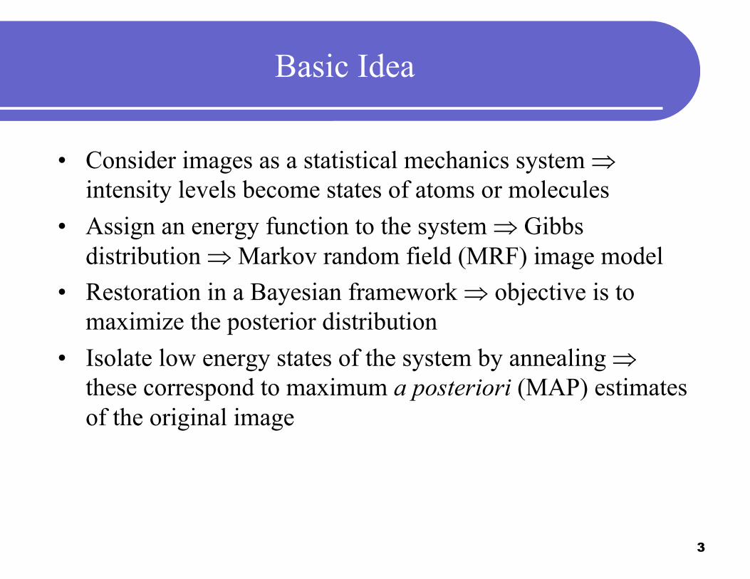
Basic Idea

• Consider images as a statistical mechanics system ⇒intensity levels become states of atoms or molecules

• Assign an energy function to the system ⇒ Gibbs distribution ⇒ Markov random field (MRF) image model

• Restoration in a Bayesian framework ⇒ objective is to maximize the posterior distribution

• Isolate low energy states of the system by annealing ⇒these correspond to maximum a posteriori (MAP) estimates of the original image

4

A Priori Image Model

• Hierarchical (layered stochastic processes for various image attributes)

• Image model: , where– F: matrix of pixel intensities (intensity process)– L: dual matrix of edge elements (line process)

• A priori knowledge is captured by distribution

5

Degraded Image Model

• Degraded images: with , where– H: blurring– : nonlinear distorsion– : invertible operation (e.g. addition, multiplication)– N: noise (Gaussian, with mean and std. dev. )

• Requirement: F and N (also L and N) are independent

6

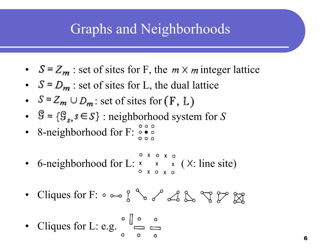
Graphs and Neighborhoods

• : set of sites for F, the integer lattice• : set of sites for L, the dual lattice• : set of sites for• : neighborhood system for S• 8-neighborhood for F:

• 6-neighborhood for L: ( : line site)

• Cliques for F:

• Cliques for L: e.g.

7

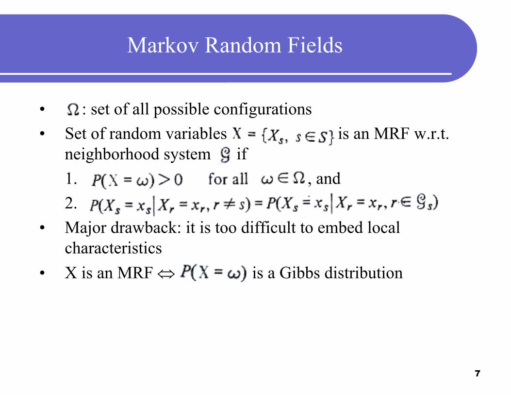
Markov Random Fields

• : set of all possible configurations• Set of random variables is an MRF w.r.t.

neighborhood system if1. , and2.

• Major drawback: it is too difficult to embed local characteristics

• X is an MRF ⇔ is a Gibbs distribution

8

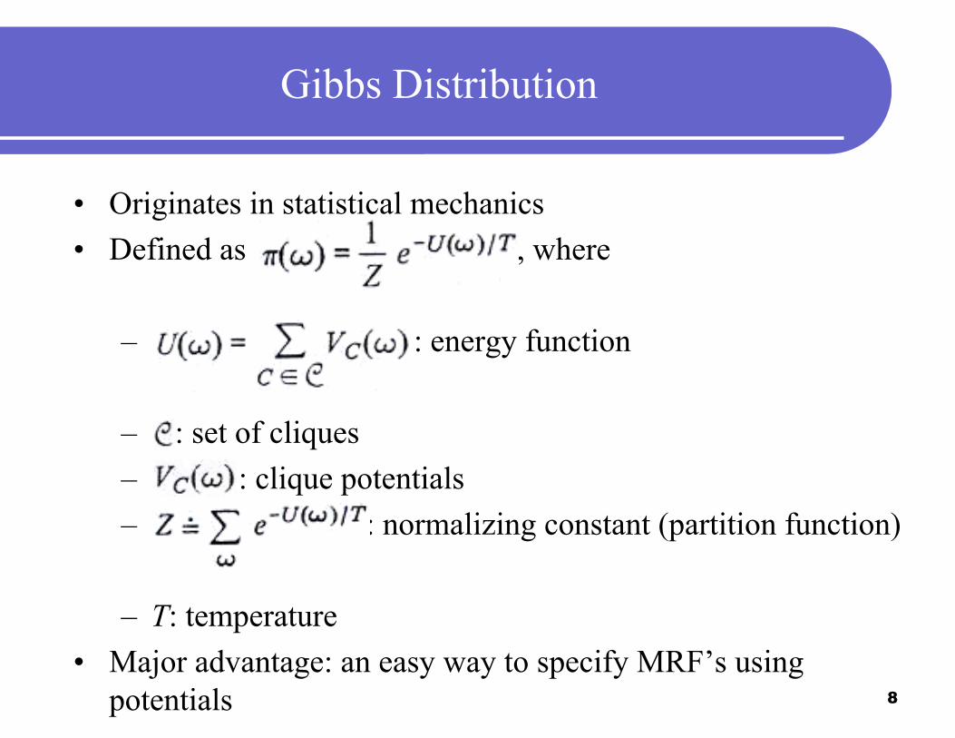
Gibbs Distribution

• Originates in statistical mechanics• Defined as , where

– : energy function

– : set of cliques– : clique potentials– : normalizing constant (partition function)

– T: temperature• Major advantage: an easy way to specify MRF’s using

potentials

9

Restoration Algorithm

• Bayesian framework• Objective function is the posterior distribution

• and are Gibbsian• The distribution of G need not be known• Maximize the objective function to get a maximum a

posteriori (MAP) estimate of the original image• | | is huge ⇒ optimization is based on stochastic

relaxation, Gibbs sampler and simulated annealing

10

Stochastic Relaxation

• A nondeterministic, stochastic, iterative algorithm to find one of the lowest energy states of a mechanics system

• Based on Boltzmann distribution: , where– : potential energy– with K denoting Boltzmann’s constant

• At iteration t a new configuration is generated from as follows:1. Choose a random configuration2. is accepted with probability ,

where3. is set to or depending on q

11

Gibbs Sampler I.

• A stochastic relaxation algorithm, which generates new configurations from a given Gibbs distribution

• Used– to generate samples from , and– to minimize the objective function

• Supports parallel computation• At iteration t the new configuration is chosen from

using the local characteristics (neighborhood) of site s• At most one site undergoes a change for every t• Sites are visited in a fixed order• The result does not depend on• The distribution of converges to

12

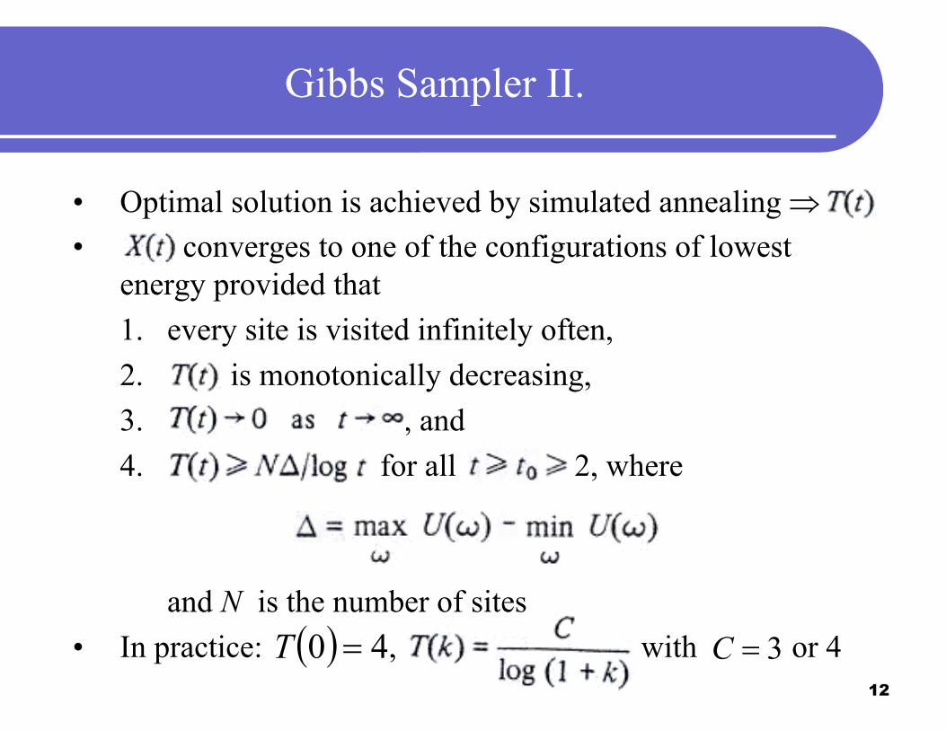
Gibbs Sampler II.

• Optimal solution is achieved by simulated annealing ⇒• converges to one of the configurations of lowest

energy provided that1. every site is visited infinitely often,2. is monotonically decreasing,3. , and4. for all 2, where

and N is the number of sites• In practice: , with or 4( ) 40 =T 3=C

13

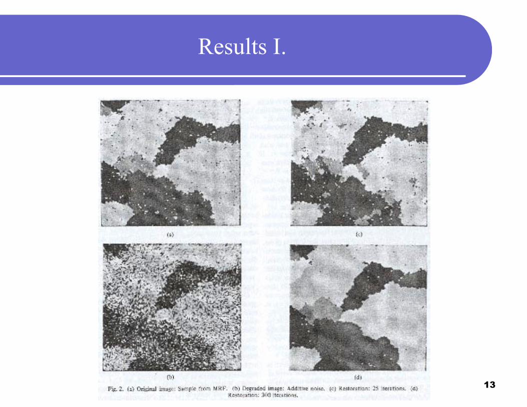
Results I.

14

Results II.

15

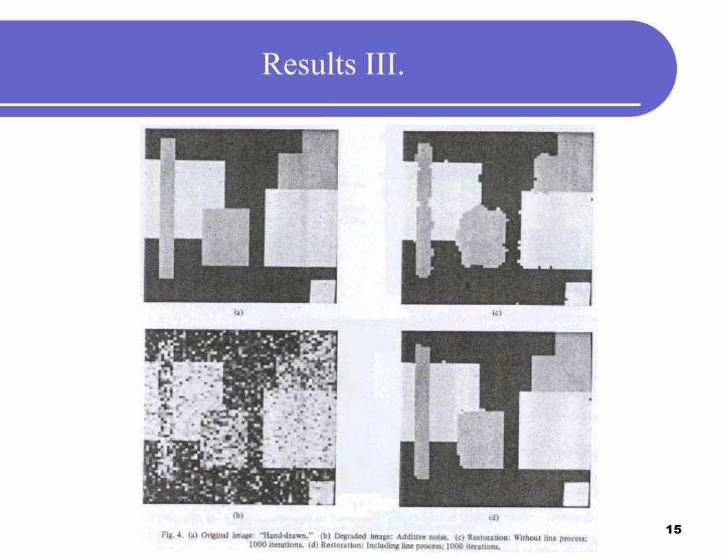
Results III.

16

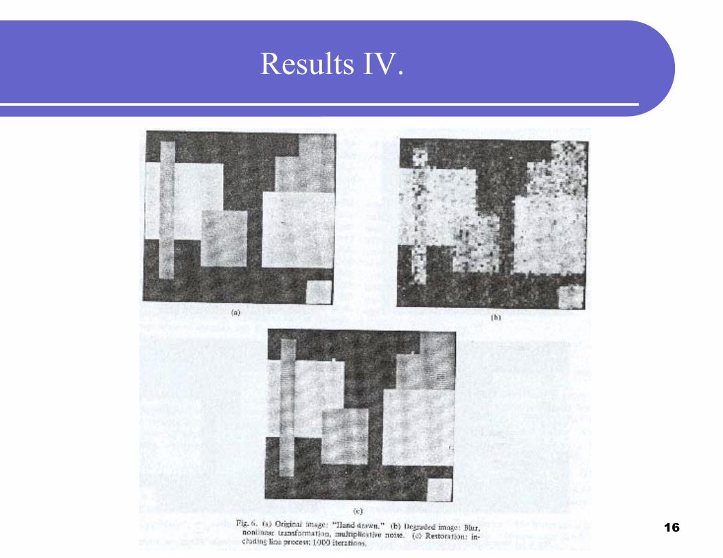
Results IV.

17

Results V.