AMO - Advanced Modeling and Optimization, Volume 5, Number 1, 2003

Stochastic Programming Models in Financial Optimization:A Survey1

Li-Yong YU Xiao-Dong JI Shou-Yang WANG2

Institute of Systems ScienceAcademy of Mathematics and Systems Sciences

Chinese Academy of sciencesBeijing 100080, People’s Republic of China

Abstract: In this paper, we survey the stochastic programming models developedto deal with financial optimization problems. A few methods are introduced indetails to generate reasonable scenarios which are of much importance for a successfulmodel. Besides, computation aspect as well as some open problems in this area areaddressed.

Keywords: Stochastic Programming, Financial Optimization, Risk Management,Scenario Generation

1 Introduction

Financial optimization is one of the most attracting areas in decision-making under uncertainty.Prominent examples include: 1)asset allocation for pension plans and insurance companies; 2)se-curity selection for stock and bond portfolio managers; 3)currency hedging for multi-nationalcorporations; 4)hedge fund strategies to capitalize on market conditions; 5)risk management forlarge public corporations. In these situations, time periods and uncertainties play importantroles. For example, a pension plan must focus on both the long-term and short-term conse-quences of his investment strategy. He must attempt to minimize pension contribution expensesover time, while satisfying the needs of the retirees, and reducing risks. Besides, there are manyuncertainties in financial planning problems, such as economic factors, prices of the securitiesconsidered, amount of cash flows, etc.. To capture both these aspects, multi-stage stochasticprogramming models are well suited to address significant practical issues.

Stochastic programming (SP) models have been proposed and well studied since late 1950sby Dantzig[1][2], Beale[3], Charnes and Cooper[4] and others. They proposed a stochastic viewto replace the deterministic one, where the unknown coefficients or parameters are random withassumed probability distribution that is independent of the decision variables. Over these years,progress in computational methods is impressive and large scale problems can be efficientlysolved with high reliability (Lustig et al.,1991[22]; Bixby et al., 1992[6]; Levkovitz and Mitra,1993[7]; Mulvey et al.,1995[8]). It is these advances that have progressively made SP techniquesapplicable to real-world problems. Moreover, high frequency data are readily available on aglobal basis, and powerful computers are also easily found to conduct the optimization search.The obstacles for applying stochastic optimization models are quickly receding.

1Supported by MADIS, CAS and NSFC2The corresponding author. Email address: sywang@iss02.iss.ac.cn

1

-666666

1 2 3time

Conditional decisions at each node

s

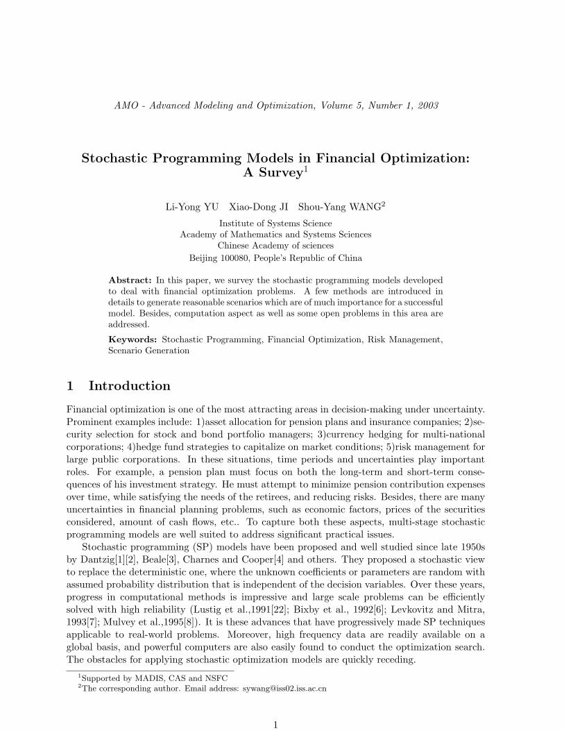
Figure 1: A scenario tree for a multi-stage stochastic program

Stochastic programming provides a general purpose-modelling framework, which captures thereal-world features such as turnover constraints, transaction costs, risk aversion, limits on groupsof assets and other consideration. However, the optimization model turns out to be intractablefor the enormous number of decision variables, especially for the multi-stage problems. Figure1 presents an example of a scenario tree whereby the decisions expand exponentially with timeperiods. Each node in this tree depicts a juncture for rendering decisions. A scenario, a completepath from the root node to a leaf, defines a single realization of the set of random variables.

The paper is organized as follows. Basic stochastic programming models and related ap-plications in financial optimization are introduced in sections 2 and 3 respectively. Section 4is dedicated to the scenario generation and computation aspect is addressed in section 5. Thecomparison with other methods is listed in section 6 and we conclude the paper with openproblems in this field.

2 Basic Stochastic Programming Models

The anticipative and the adaptive models are special cases of stochastic programs. The combi-nation of them makes a recoursive model which is widely applied in financial field.

2.1 Anticipative models

Anticipative model is also referred to as static model, for which the decision does not dependin any way on future observations of the environment. The prudent planning has to take intoaccount all possible future realizations since there is no opportunity to adapt decisions later on,which may lead to overly conservative decisions.

In anticipative models feasibility is expressed in terms of probabilistic (or chance) constraints.For example, a reliability level α, where 0 < α ≤ 1, is specified and constraints are expressed inthe form

Pω|fj(x, ω) = 0, j = 1, 2, ..., n ≥ α,

2

where x is the m−dimensional vector of decision variables and fj : Rm × Ω → R, j = 1, 2, ..., n.The objective function may also be of a reliability type, such as Pω|f0(x, ω) ≤ γ, wheref0 : Rm × Ω → R

⋃+∞ and γ is a constant.An anticipative model selects a policy that meets desirable characteristics of the constraints

and the objective function. In the example above, it is desirable that the probability of a con-straint violation is less than the prespecified threshold value 1−α. The precise value of α dependson the application at hand, the cost of constraint violation, and other similar considerations.

2.2 Adaptive models

In an adaptive model, information related to the uncertainty becomes partially available beforedecision making, so optimization takes place in a learning environment, which is the essentialdifference with an adaptive model. Let A be the collection of all the relevant informationavailable through observation, which is a subfield of all possible events. The decision x dependson the events that can be observed, and x is termed A-adapted or A-measurable. An adaptivestochastic program can be formulated as:

Minimize E[f0(x(ω), ω)|A]subject to E[fj(x(ω), ω)|A] = 0 j = 1, 2, ..., n (2.1)

x(ω) ∈ X almost surely

The mapping x : Ω → X is such that x(ω) is A-measurable. This problem can be addressed bysolving for every ω the following deterministic programs:

Minimize E[f0(x, ·)|A](ω) (2.2)subject to E[fj(x, ·)|A](ω) = 0 j = 1, 2, ..., n (2.3)

x ∈ X (2.4)

The two extreme cases, complete information and no information at all, deserve specialmention. The latter reduces the model to the anticipative form while the former is known asdistribution model, which characterizes the distribution of the optimal objective value. However,the most interesting and valuable situation arises when partial information is available, whichis what we will discuss below.

2.3 Recourse models

The recoursive model combines the former two models in a common mathematical framework,which seeks a policy that not only anticipates future observations but also takes into accounttemporarily available information to make recourse decisions. For example, a portfolio managerconsiders both future movements of stock prices (anticipation) as well as rebalancing the portfoliopositions as prices change (adaptation).

The two-stage stochastic programming problem with recourse can be written as follows:

Minimize f(x) + E[Q(x, ω)]subject to Ax = b (2.5)

x ∈ Rm0+

3

where x is the first-stage anticipative decisions, which is made before the random variables areobserved, and Q(x, ω) is the optimal value, for any given Ω, of the following nonlinear program

Minimize q(y, ω)subject to W (ω)y = h(ω)− T (ω)x (2.6)

y ∈ Rm1+

where y is the second-stage adaptive decisions, which depends on the realization of the first-stagerandom vector. q(y, ω) denotes the second-stage cost function, and T (ω),W (ω), h(ω)|ω ∈ Ωare model parameters with reasonable dimensions. Those parameters are functions of the randomvector ω and are, therefore, random parameters. T is the technology matrix containing thetechnology coefficients that convert the first-stage decision x into resources for the second-stageproblem. W is the recourse matrix and h is the second-stage resource vector.

Generally the two-stage recourse model can be formulated as follows:

Minimize f(x) + E[ miny∈Rm1

+

q(y, ω)|T (ω)x + W (ω)y = h(ω)]

subject to Ax = b (2.7)x ∈ Rm0

+

2.4 Deterministic equivalent formulation

We consider now the case where the random vector ω has a discrete and finite distribution, withsupport Ω = ω1, ω2, ..., ωN. In this case the set Ω is called a scenario set. Denote by pl theprobability of realization of the lth scenario ωl. It is assumed that pl > 0 for all ωl ∈ Ω, andthat

∑Nl=1 pl = 1.

The expected value of the second-stage optimization problem can be expressed as

E[Q(x, ω)] =N∑

l=1

plQ(x, ωl). (2.8)

For each realization of the random vector ωl ∈ Ω a different second-stage decision is made,which is denoted by yl. The resulting second-stage problems can then be written as:

Minimize q(yl, ωl)subject to W (ωl)yl = h(ωl)− T (ωl)x, (2.9)

yl ∈ Rm1+ .

Combining now (2.8) and (2.9) we reformulate the stochastic nonlinear program (2.7) as thefollowing large-scale deterministic equivalent nonlinear program:

Minimize f(x) +N∑

l=1

plq(yl, ωl) (2.10)

subject to Ax = b, (2.11)T (ωl)x + W (ωl)yl = h(ωl) for all ωl ∈ Ω, (2.12)x ∈ Rm0

+ , (2.13)

yl ∈ Rm1+ . (2.14)

4

2.5 Multistage models

The recourse problem is not restricted to the two-stage formulation. It is possible that obser-vations are made at T different stages and are captured in the information sets AtT

t=1 withA1 ⊂ A2 · · · ⊂ AT . Stages correspond to time instances when some information is revealed anda decision can be made. (Note that T is a time index, while T (ω) are matrices.)

A multistage stochastic program with recourse will have a recourse problem at stage τconditioned on the information provided by Aτ , which includes all information provided by theinformation sets At, for t = 1, 2, ..., τ . The program also anticipates the information in At, fort = τ + 1, ..., T .

Let the random vector ω have support Ω = Ω1×Ω2×· · ·×ΩT , which is the product set of allindividual support sets Ωt, t = 1, 2, ..., T . ω is written componentwise as ω = (ω1, ..., ωT ). De-note the first-stage variable vector by y0. For each stage t = 1, 2, ..., T , define the recoursevariable vector yt ∈ Rmt , the random cost function qt(yt, ωt), and the random parametersTt(ωt),Wt(ωt), ht(ωt)|ωt ∈ Ωt.

The multistage program, which extends the two-stage model (2.7), is formulated as thefollowing nested optimization problem

Minimize f(y0) + E

[min

y1∈Rm1+

q1(y1, ω1) + . . . E

[min

yT∈RmT+

qT (yT , ωT )

]. . .

]

subject to T1(ω1)y0 + W1(ω1)y1 = h1(ω1), (2.15)...TT (ωT )yT−1 + WT (ωT )yT = hK(ωT ),y0 ∈ Rm0

+ .

For the case of discrete and finitely distributed probability distributions it is again possibleto formulate the multistage model into a deterministic equivalent large-scale nonlinear program.

3 Stochastic Programming Models in Financial Optimization

Lots of articles in the literature have illustrated that stochastic programming models are flexibletools to describe financial optimization problems under uncertainty with realistic market imper-fections and trading restrictions. Bradley and Crane (1972)[9] and Kusy and Zeimba (1986)[10]describe stochastic linear programs for bank asset/liability management, Carino et al.(1994)[11]formulate the asset/liability management problem of a Japanese insurance company as a mul-tiperiod stochastic linear program, Mulvey and Vladimirou(1992)[12] propose a multiperiodstochastic network model for the purpose of asset allocation, and Hiller and Eckstein(1993)[13],Zenios(1993)[36], and Golub et al.(1993)[15] describe stochastic programming models for fixed-income securities management.

In the following, we introduce some application of stochastic programming models in financialoptimization.

3.1 Stochastic Programming Model for Asset Allocation Problem

Asset allocation problem can be viewed as multiperiod dynamic decision problems where trans-actions take place at discrete time points.To define the model, we divide the entire planninghorizon T into two discrete time intervals T1 and T2, where T1 = 0, 1, ..., τ and T2 = τ + 1, ..., T .

5

The former corresponds to periods in which investment decisions are made. Period τ defines thedate of the planning horizon; we focus on the investor’s position at the beginning of period τ .Decisions occur at the beginning of each time stage. Much flexibility exists. An active tradermight see his time interval as short as minutes, whereas a pension plan advisor will be moreconcerned with much longer planning periods such as the dates between the annual Board ofDirector’s meeting. It is possible for the steps to vary over time - short intervals at the beginningof planning period and longer intervals towards the end. T2 handles the horizon at time τ bycalculating economic and other factors beyond period τ up to period T . The investor cannotrender any active decisions after the end of period τ .

Asset investment categories are defined by set A = 1, 2, ..., I, with category 1 representingcash. The remaining categories can include broad investment groupings such as stocks, bonds,and real estate. The categories should track well-defined market segments. Ideally, the co-movements between pairs of asset returns would be relatively low so that diversification can bedone across the asset categories.

In the model, uncertainty is represented by a set of distinct realization s ∈ S. Scenarios mayreveal identical value for the uncertain quantities up to a certain period. Scenarios that sharecommon information must yield the same decisions up to that period.

We assume that the portfolio is rebalanced at the beginning of each period. Alternatively,we could simply make no transaction except reinvest any dividend and interest—a buy and holdstrategy. For convenience, we also assume that the cashflows are reinvested in the generatingasset category and all the borrowing is done on a single period basis.

For each i ∈ A, t ∈ T1, and s ∈ S, we define the following parameters and decision variables.Parameters:

rsi,t =1 + ρs

i,t, where ρsi,t is the percent return for asset i, time period t, under scenario s

(projected by the stochastic scenario generator, for example, see Mulvey et al. 1999 [16]).

πs Probability that scenario s occurs,∑S

s=1 πs = 1.

w0 Wealth in the beginning of time period 0.

σi,t Transaction costs incurred in rebalancing asset i at the beginning of time period t (sym-metric transaction costs are assumed, i.e., cost of selling equals cost of buying).

βst Borrowing rate in period t under scenario s.

Decision variables:

xsi,t Amount of money for asset category i, in time period t, under scenario s, after rebalancing.

vsi,t Amount of money in asset category i, in the beginning of time period t, under scenario s,

before rebalancing.

wst Wealth at the beginning of time period t, under scenario s.

psi,t Amount of asset purchased for rebalancing in period t, under scenario s.

dsi,t Amount of asset i sold for rebalancing in period t, under scenario s.

bst Amount of money borrowed in period t, under scenario s.

6

Given these definitions, we present a general stochastic programming model in financialoptimization.

Model SP

Maximize Z =S∑

s=1

πsf(wsτ ) (3.1)

Subject to∑

i

xsi,0 = w0 ∀s ∈ S, (3.2)

∑

i

xsi,τ = ws

τ ∀s ∈ S, (3.3)

vsi,t = rs

i,t−1xsi,t−1 ∀s ∈ S, t = 1, ..., τ, i ∈ A, (3.4)

xsi,t = vs

i,t + psi,t(1− σi,t)− ds

i,t ∀s ∈ S, i 6= 1, t = 1, ..., τ, (3.5)

xs1,t = vs

1,t +∑

i6=1

dsi,t(1− σi,t)−

∑

i6=1

psi,t − bs

t−1(1 + βst−1) + bs

t

∀s ∈ S, t = 1, ..., τ, (3.6)xs

i,t = xs′i,t for all scenarios s and s′ with identical past up to time t. (3.7)

As with the single-period models, the nonlinear objective function (3.1) can take severaldifferent forms. If the classical return-risk function is employed, then (3.1) becomes Max Z = ηMean(wτ )− (1− η)Risk(wτ ), where Mean(wτ ) is the expected total wealth and Risk(wτ ) is therisk of the total wealth across the scenarios at the end of period τ . Parameter η indicates therelative importance of risk as compared with the expected value. This objective leads to anefficient frontier of wealth at period τ by allowing alternative values of η in the range [0,1]. Analternative to mean-risk is the von Neumann-Morgenstern expected utility of wealth at period τ .Here, the objective becomes MaxZ =

∑Ss=1 πsUtility(ws

τ ) where Utility(W) is the Von MeumannMorgenstern utility function. Other objective functions are possible, such as the one proposedby Zhao and Zeimba[17].

Constraint (3.2) guarantees that the total initial investment equals the initial wealth. Con-straint (3.3) represents the total wealth at the beginning of period τ . This constraint can bemodified to include assets, liabilities, and investment goals. The modified result is called thesurplus wealth(Muvey,1989 [18]). Most investors render investment decisions without referenceto liabilities or investment goals. Mulvey employs the notion of surplus to the mean-varianceand the expected utility models to address liabilities in the context of asset allocation strate-gies. Constraint (3.4) depicts the wealth vs

i,t accumulated at the beginning of period t beforerebalancing in asset i. The flow balance constraint for all assets except cash for all periods isgiven by constraint (3.5). This constraint guarantees that the amount invested in period t equalsthe net wealth for asset. Constraint (3.6) represents flow balancing constraint for cash. Non-anticipativity constraints are represented by (3.7). These constraints ensure that the scenarioswith the same past will have identical decisions up to that period. While these constraints arenumerous, solution algorithms take advantage of their simple structure.

Model (SP) is a split variable formulation of stochastic asset allocation problem. This formu-lation has proven successful for solving the model using techniques such as progressive hedgingalgorithm of Rockafellar and Wets(1991)[19] and the quadratic diagonal approximation of Mul-vey and Ruszczynski(1995)[20] and Berger et al.(1994)[21]. The split variable formulation can be

7

beneficial for direct solvers that use the interior point method (Lustig, Mulvey, and Carpenter,1991[22].

By substituting constraint (3.7) back in constraint (3.2) to (3.6), we obtain a standardform of the stochastic allocation problem. Constraints for this formulation exhibit a dual blockdiagonal structure for two stage stochastic programs and a nested structure for general multi-stage problems. This formulation may be better some direct solvers. The standard form of thestochastic program possesses fewer decision variables than the split variable model and is thepreferred structure by many researchers in the field. This model can be solved by means ofdecomposition methods, for example, the L-shaped method (a specialization of Benders algo-rithm). See Birge and Loveaux(1997)[23], Dantzig and Infanger(1993)[24], Dempster(1998)[25],Infanger(1994)[26], and Kall and Wallace(1994)[27] and their numerous references.

The multi-stage model can provide superior performance over single period models. See thereferences(Berger and Mulvey 1996[28], Carino et al.1994[11], Dempster 1998[25], Dert 1995[29],Holmer 1994[30], Klaassen 1994[31] and 1998[60], Mulvey and Zeimba 1995[33], Nielsen andZenios 1996[34], Worzel et al. 1995[35], and Zenios 1993[36]).

3.2 Stochastic Programming Models for the Management of Fixed-incomeSecurities

The new fixed-income securities, including high-yield bonds, mortgage-backed securities, callablebonds, and international bonds have been developing rapidly in recent years. Compared to thetraditional portfolio optimization, the management of fixed-income securities have to cope withmore uncertainties, so is more complex.

The management of fixed-income securities can be viewed as a multistage decision problemin which portfolio actions are taken at successive (discrete) points in time. At each decisionperiod, the portfolio manager has an inventory of securities and/or cash on hand. Based uponpresent credit market conditions and his assessment of future interest rates and cash flows, themanager must decide which securities to hold in the portfolio over the next time period, whichsecurities to sell, and which securities to purchase from the market. These decisions are madesubject to a constraint on total portfolio size, which may be larger or smaller than the previousperiod’s constraint depending upon whether a cash inflow or outflow occurred. At the nextdecision period, the portfolio manager faces a new set of interest rates and a new portfolio sizeconstraint. He must then make another set of portfolio decisions which take into account thenew information. This decision-making process, which is repeated over many time periods, isdynamic in the sense that the optimal first period decision depends upon the actions which willbe taken in each future period for each uncertain event.

Any proposed model for the management of fixed-income securities should be able to copewith the uncertainties inherent in those securities. Bennett Golub et al.[37] pointed that thereare two major sources of uncertainty in the new fixed-income markets, in addition to the usualinterest rate risk. First, is the timing and amount of cash flows received from the securities.Second, is the spread over the risk-free rate that prices the security. This spread reflects premiaon risk factor that are present in the specific fixed-income market, but are absent from Treasurysecurities. The timing of the cash flows depends on the embedded (or real) options of thesecurity. For example, corporate bonds may be called prior to maturity. The loans backing amortgage security may prepay or default.

In the absence of market imperfections, dynamic portfolio investment problems have beenstudied using continuous-time models, usually in the context of an individual who maximizesexpected utility of future consumption(c.f. Cox and Huang 1989 [38]). These models can be

8

solved analytically if the state variables are assumed to follow diffusion process and certainrestrictions are imposed on the form of the utility function. In practice, the applications ofthese models are restricted for the number of risky and riskless assets to be analyzed is limited.

For portfolio investment problem of practical importance, one has no choice but to usestochastic programming models in which both time and the state space are discretized. Animportant contribution in multi-period dynamic models was made by Bradley and Crane [9], whoproposed a stochastic programming models with recourse for bond management. Their modelallows the full spectrum of interest rate and price changes, and permits portfolio rebalancing.After that, much work has been done in this field. For example, Zenios [39] proposed a modelfor managing portfolios of mortgage-backed securities. Bennett Golub [40] developed a multi-period dynamic portfolio optimization model to address the problem of management of fixed-income securities. Christiana Vassiadou-Zeniou and Stavros A. Zenios [41] presented a multi-stage stochastic program with recourse for the management of portfolios of callable bonds. Inthese models, stochastic programs are used to address the time and uncertainty in financialplanning. To illustrate this in detail, we introduce the model of Andrea Beltratti et al.[42] forthe management of international bond portfolios.

To the problem of portfolio management in the international markets, there are three aspectsthat need our consideration, interest rate risk in the local market, exchange rate volatility acrossmarkets, and decisions for hedging currency risk. In this model these decisions are integratedin a common framework, while in the past they were addressed separately. In order to getnecessary data to realize the model, Monte Carlo simulation procedures are used to generatejointly scenarios of interest and exchange rates.

Now we give a detailed description of the problem. In this portfolio management problem, theaim is to manage a bond portfolio in a way that it tracks a broadly defined international marketindex. The indexation tracking strategy is widely used by insurance and pension fund companies,foundations, and money management firms. A bond index in each market i = 1, 2, ..., m, isconstructed by creating a representative sample Φi of size Ni from the universe of eligible bondsΩi. For each security j = 1, 2, ..., Ni, in the representative set, the index specifies its relativeweight φi

j which reflects the capitalization structure of the universe set Ωi with bonds that havecharacteristics identical or similar to the jth bond. The global bond index is represented by aset Γ of country indices and the relative weights γi assigned to the bond index of each countrybased on the market value of the different indices. These weights are a measure of the share ofthe bond market of the ith country in the world bond market.

The manager of an international bond portfolio must determine the fraction of the portfoliovalue invested in each of the m markets, and to pick specific bonds from each market Ωi to adjustthe portfolio. These decisions are usually made in three steps. An asset allocation committeedetermines first the exposure of the portfolio to each market. Then traders identify mispricedbonds in each market and construct the country-specific portfolio. Finally, once the country-specific funds are constructed the currency exposure may be hedged.

Now we present the integrative model for tracking an international fixed income index.The interesting contribution of the model is that it combines the following three aspects in

an integrated fashion, i.e. asset allocation in different markets, bond picking in each market,and optimal currency hedging ratios.The model specifies optimal bond picking decisions in eachof the m markets to track the global index.

Integrative model: First-stage constraints

9

The first stage (i.e. at time t0) cashflow accounting equation of the model is:

c0 +m∑

i=1

e0i

Ni∑

j=1

ζi0j

Y i0j

=m∑

i=1

e0i

Ni∑

j=1

(ζi0j

+ δ)Xi0j

+ v0. (3.8)

The inventory balance constraint is:

bi0j

+ Xi0j

= Y i0j

+ Zi0j

for all i ∈ Γ and j ∈ Φi. (3.9)

For the sake of simplicity we assume here that all sales and purchases are made into and from thebase currency (in which investor measures his return), thus avoiding the need to keep separatecashflow variables.

Integrative model: Time-staged constraints

Cashflow accounting constraints of the model at any time period t after t = 0 depend on thepath lt. These constraints limit the increase in holdings for each bond in each market.

There is one constraint for each path lt ∈ Pt (the arguments lt are dropped from all variablesand parameters below for simplicity of notation):

ρt−1vt−1 +m∑

i=1

eti

Ni∑

j=1

kit−1j

Zit−1j

+m∑

i=1

eti

Ni∑

j=1

ζitjY

itj

=m∑

i=1

eti

Ni∑

j=1

(ζitj + δ)Xi

tj + vt. (3.10)

Inventory balance equations constrain the amount of each bond sold or remaining in theportfolio to be equal to the outstanding amount at the end of the holding period, plus anyadditional amount purchased. There is one constraint for each bond and for each path lt ∈ Pt:

Zit−1j

+ Xitj = Y i

tj + Zitj for all i ∈ Γ, j ∈ Φi. (3.11)

Integrative model: objective function

At the end of the planning horizon T and for each path lT ∈ PT we calculate the return ofthe portfolio. This value depends on the composition of the portfolio and the value of the bondsat T and on any accrued cashflow from previous periods. The return of the portfolio is given by

Rp(lT ) .= Rp(ZT (lT )) =vT +

∑mi=1 eTi

∑Nij=1 ζi

TjZi

Tj− Vp0

Vp0, (3.12)

where Vp0 is the initial value of the portfolio.For our aim is to track the market indexation, the objective function maximizes the expected

utility of excess return of the portfolio over the index,

Maximize∑

lT∈PT

πlTU(

Rp(lT )IT (lT )

), (3.13)

10

where U(·) denotes the utility function. Here we choose to maximize a utility function of excessreturn to allow for tradeoffs of growth versus security, which was addressed by MacLean, Ziembaand Blazenko (1992) [43]. Choosing for instance a logarithmic utility function we can implementin our model the investor’s wish to follow a growth optimal strategy over the long run.

Optimal currency hedging ratios

Hedging decision in the optimization model can now be incorporated. Define a new variable(H0i)

mi=1 to denote the amount of each currency hedged at agreed upon 1-period forward rates

(f0i)mi=1 at period t = 0. Let also (Hti(lt))

mi=1 denote the amount hedged at forward rates

(fti(lt))mi=1 at period t under path lt.

The cashflow accounting constraints must be modified to account for the fact that at eachperiod t an amount Hti(lt) of the i currency will be exchanged at rate fti(lt) and any remainingamount will be exchanged at rate eti(lt). Recall that there is one constraint for each path lt ∈ Pt,and that the arguments lt are dropped from all variables and parameters below for simplicity ofnotation.

The total cashflow in the ith currency—inflows from coupon payments and security salesand outflows from security purchase—at period t under scenario lt is given by

wti =Ni∑

j=1

kit−1j

Zit−1j

+Ni∑

j=1

ζitjY

itj −

Ni∑

j=1

(ζitj + δ)Xi

tj (3.14)

The cashflow accounting equation (13) is rewritten to incorporate hedging as:

ρt−1vt−1 +m∑

i=1

(ft−1iHt−1i + eti(wti −Ht−1i)) = vt. (3.15)

At the end of the planning horizon the return of the portfolio—in the base currency—willbe a function of the amount hedged and the forward and current exchange rates. The returncalculation takes the form:

Rp(lT ) .= Rp(ZT (lT )) = (3.16)

vT +∑m

i=1

(fT−1i

HT−1i+ eTi

(∑Nij=1 ζi

jZiTj−HT−1i

))− Vp0

Vp0

In order to implement the portfolio optimization models we need a simulation procedureto generate interest rate and exchange rate scenarios. Once such scenarios are generated thecalculation of bond price conditioned on the observed interest rates is straightforward; see , e.g.,Mulvey and Zenios (1994) [44].

3.3 Stochastic Programming Models for Asset/Liability Management

Asset/Liability management(ALM) addresses the problem of an investor who faces a sequenceof liability payments in the future, and wants to construct a portfolio of securities that allowshim to meet these liabilities under a variety of plausible scenarios. From all feasible portfolioshe wants to choose the one that optimizes some optimality criterium (e.g.,minimum cost). Boththe size of the liability payments and the security returns may depend on the state of the worldin the future. This problem can be modelled as a multi-period stochastic linear program, which

11

explicitly includes the possibility of portfolio rebalancing at future points in time as responseto new information that becomes available. As we are interested in presenting a modellingframework for realistic ALM problems, market imperfections and trading restrictions are takeninto account.

In recent years the number of publications about stochastic programming for asset liabilitymanagement has risen drastically, probably inspired by the rapid increase of efficiency andaccessibility of computer systems. Some of the applications are very successful. For example, theinsurance ALM model of Carino and Zeimba[45] has been extensively used by the Frank Rusellcompany in consulting ALM managers in insurance and pension fund. Their work with TheYasuda Fire and Marine Insurance Company was a finalist at the Franz Edelman Competitionfor Management Science Achievements. Similar acclaim was achieved by the Towers Perrin-Tillinghast model of Mulvey, Gould and Morgan [46]. Stochastic programming models for Dutchpension funds were developed by Dert [47], a general ALM model for insurers by Consigli andDempster [48].

Now we introduce the model presented by Klaassen [60].In asset/liability management one generally faces a trade-off between the initial cost of the

asset portfolio of which the payoffs must be sufficient to meet the liabilities, and the value ofthe portfolio that is left at the end of the model horizon. Although we have assumed that theinvestor can borrow money at intermediate trading dates, we require that the final portfoliovalue must be nonnegative in all scenarios. The trade-off between the initial investment and thevalue of the portfolio at the end of the model horizon is captured in the objective function: theinitial portfolio investment is minimized, but any positive final portfolio value is credited to theobjective using a concave utility function U(·). We assume that this utility function satisfies theexpected utility property.

The ALM problem can now be formulated as the following multiperiod stochastic program.

minimize (1 + c)I∑

i=1

Si,0xbi,0 − (1− c)I∑

i=1

Si,0xsi,0

+P0y0 − e−κ∆P0z0 −∑

s∈ST

ηsTU(ys

T ) (3.17)

subject to−xsi,0 + xbi,0 − xhi,0 = −xi,0 ∀i = 1, ..., I, (3.18)

xhs−i,t−1 − xss

i,t + xbsi,t − xhs

i,t = 0∀i = 1, ..., I, s ∈ St, t = 1, ..., T − 1, (3.19)

I∑

i=1

Dn(s)i,t xhs−

i,t−1 + ys−t−1 − zs−

t−1 + (1− c)I∑

i=1

Sn(s)i,t xss

i,t

−(1 + c)I∑

i=1

Sn(s)i,t xbs

i,t − Pn(s)t ys

t + e−κ∆Pn(s)t zs

t = Ln(s)t

∀s ∈ St, t = 1, ..., T − 1, (3.20)

12

I∑

i=1

(Dn(s)i,T + S

n(s)i,T )xhs−

i,T−1 + ys−T−1 − zs−

T−1 − ysT = L

n(s)T

∀s ∈ ST , (3.21)xss

i,t, xbsi,t, xhs

i,t ≥ 0∀i = 1, ..., I, s ∈ St, t = 0, ..., T − 1, (3.22)ys

t ≥ 0 ∀s ∈ St, t = 0, ..., T, (3.23)

0 ≤ zst ≤ Z

n(s)t ∀s ∈ St, t = 0, ..., T − 1. (3.24)

We will refer to this formulation as the ALM model.The first four terms in the objective function represent the net cost of additional investments

at time 0. These additional investments consist of asset purchases (including transaction costs)and investment in the riskless one period security, while revenues from the sale of assets (net oftransaction costs) and borrowing are subtracted. The last term in the objective is the expectedutility of a final portfolio surplus.

We distinguish between three types of constraints in the model: portfolio-balance constraints,cash-balance constraints and borrowing constraints. The portfolio-balance constraints link port-folio holdings between successive periods (ie., before and after rebalancing) in each scenario andfor each asset. The portfolio-balance constraints are given by (3.18) for all assets at time 0, andby (3.19) for all assets in each scenario after time 0.

The cash-balance constraints make sure that sufficient cash is generated to meet the liabilitypayment in each scenario at each time. For each scenario at time t < T , this constraint isgiven by (3.20). At the end of a period , the investor receives dividend payments on his assetholdings and the return on his investment in the one period riskless security but has to repay theamount borrowed in the previous period plus interest (represented by the first three terms onthe left-hand side of (3.20)). The next two terms reflect rebalancing of the portfolio: revenuesare generated by selling assets, and money can be invested by buying assets, where both areadjusted for transaction costs. The final two terms on the left-hand side are the investment inthe riskless one period security and the amount borrowed, respectively, during the next period.

The cash-balance constraints (3.21) at time T define the final portfolio value in each scenario.The first three terms on the left-hand side determine the final portfolio value before meeting theliability: the portfolio holdings are converted at the current market prices, the return on theinvestment in the riskless one period security is added, and the amount due because of borrowingsubtracted. The difference between this portfolio value and the liability payment in a scenarios ∈ ST is the final portfolio surplus ys

T .The nonnegativity restriction on xhs

i,t prevent short sales of assets, while Equation (3.24)states the upper bounds on borrowing.

4 Scenario Generation

To operate the stochastic programming models, scenarios generation and constructing eventtrees are of very importance. We describe some methods that have been proposed to deal withthese two problems. In constructing event trees, arbitrage-free condition should be noted.

4.1 Methods for Generating Scenarios

In this subsection we describe three specific methods for generating asset return scenarios withmore detail: (i) bootstrapping historical data, (ii) statistical modelling with the Value-at-Risk

13

approach, and (iii) modelling economic factors and asset returns with vector autoregressivemodels.

4.1.1 Bootstrapping historical data

The simplest approach for generating scenarios use only the available data without any mathe-matical modelling. It bootstraps a set of historical records. Each scenario is a sample of assetsreturns which is obtained by sampling returns that were observed in the past. Dates from theavailable historical records are selected randomly and for each date in the sample we read thereturns of all asset classes or risk factors during the month prior to that date. These are sce-narios of monthly returns. If we want to generate scenarios of returns for a long horizon—say1 year—we sample 12 monthly returns from different points in time. The compounded returnof the sampled series is the 1-year return. Note that with this approach the correlations amongasset classes are preserved.

4.1.2 Statistical models from the Value-at-Risk literature

Time series analysis of historical data can be used to estimate volatilities and correlation matricesamong asset classes of interest. These correlation matrices are used to measure risk exposure ofa position through the Value-at-Risk (VaR) methodology.

Denote the random variables by the K-dimensional random vector ω. The dimension of ω isequal to the number of risk factors we want to model. Assuming that the random variables arejointly normally distributed we can define their probability density function of ω by

f(ω) = (2π)−p/2|Q|−1/2 exp[−1

2(ω − ω)

′Q−1(ω − ω)

], (4.1)

where ω is the expected value of ω and Q is the covariance matrix and they can be calculatedfrom historical data. (It is typically the case in financial time series to assume that the logarithmsof the changes of the random variables have the above probability density function, so that thevariables themselves follow a lognormal distribution.)

Once the parameters of the multivariate normal distribution are estimated we can use it inMonte Carlo simulations, using either the standard Cholesky factorization approach or scenariogeneration procedures based on principal component analysis discussed in Jamshidian and Zhu(1997)[50].

The simulation can be applied repeatedly at different states of an event tree. However, wemay want to condition the generated random values on the values obtained by some of therandom variables. For instance, users may have views on some of the variables, or a moredetailed model may be used in the simulation hierarchy to estimate some of the variables. Thisinformation can be incorporated when sampling the multivariate distribution.

The conditional sampling of multivariate normal variables proceeds as follows. Variable ω ispartitioned into two subvectors ω1 and ω2, where ω1 is the vector of dimension K1 of randomvariables for which some additional information is available and ω2 is the vector of dimensionK2 = K −K1 of the remaining variables. The expected value vector and covariance matrix arepartitioned similarly as

ω =

ω1

ω2

and Q =

Q11 Q12

Q21 Q22

. (4.2)

14

The marginal probability density function of ω2 given ω1 = ω1∗ is given by

f(ω2|ω1 = ω1∗) =

(2π)−p2/2|Q22.1|−1/2 exp[−1

2(ω2 − ω2.1)

′Q−1

22.1(ω2 − ω2.1)]

, (4.3)

where the conditional expected value and covariance matrix are given by

ω2.1(ω∗1) = (ω2 −Q21Q−111 µ1) + Q21Q

−111 ω∗1, (4.4)

and

Q22.1 = Q22 −Q21Q−111 Q12, (4.5)

respectively. Scenarios of ω2 for period t conditioned on values of ω1 given by ω∗1 can be generatedfrom the multivariate normal variables from (4.3) through the expression

ωt2i = ω0

2i exp[σi

√tω2i

],

where ω02i is today’s value and σi is the single-period volatility of the ith component of the

random variable ω2.Consiglio and Zenios (2001)[51] use the Riskmetrics methodology in conjunction with dis-

crete lattice models to generate joint scenarios of term-structure and exchange rates. Interestrate differences among two countries are key determinants of the exchange rate between thecurrencies. Hence, exchange rate scenarios are conditioned on the interest rates of the two cur-rencies, the base currency and the foreign currency. The standard assumption applies that thelogarithms of the ratios of exchange rates at period t to period t− 1, and the logarithms of theratios of spot interest rates at period t to period t− 1 follow a multivariate normal distribution.Daily and weekly rates do not follow normal distributions but there is lack of empirical evidenceagainst normality for monthly data such as those used by Consiglio and Zenios.

4.1.3 Scenario generation using vector autoregressive models

Vector autoregressive models are often used to generate scenarios. To illustrate this, we consideran ALM simulation system for Dutch pension funds as an example (see Boender 1997[52]). Asthe scope of ALM systems for Dutch pension funds is often limited to long term strategicdecisions, the investment model only considers a small set of broad asset classes: deposits,bonds, real estate and stocks. Apart from the returns on these assets, each scenario shouldcontain information about future wage growth in order to calculate the future values of thepension liabilities.

In order to generate asset returns and the wage growth rate a vector autoregressive modelis applied by Boender (1997):

Rt = c + V ht−1 + εt, εt ∼ N(0, Q), t = 1, 2, ..., T, (4.6)Rit = ln(1 + rit), i = 1, 2, ..., m, t = 1, 2, ..., T, (4.7)

where m is the number of asset time series, rit is the discrete rate of change of variable i inyear t, Rt is an m-dimensional vector of continuously compounded rates, c is the m-dimensionalvector of coefficients, V is an m × m matrix of coefficients, εt is the m-dimensional vector oferror terms and Q is the m×m covariance matrix.

15

The specification of the vector autoregressive model should be chosen carefully. Althoughsome inter-temporal relationships between the returns might be weakly significant based on his-torical data, that does not imply that these relationships are also useful for generating scenariosfor a financial optimization model with a long time horizon. To avoid any problems with un-stable and spurious predictability of returns, we do not use lagged variables for explaining thereturns of bonds, real estate, and stocks in the vector autoregressive model. The time series ofthe return on deposits and the increase of the wage level on the other hand are known to havesome memory, so we model them by a first order autoregressive process.

There are many ways to estimate vector autoregressive models, see, e.g., Judge et al.(1988)[53]. After the vector autoregressive model has been used to generate scenarios of as-set returns and wage growth, the liability values can be added to each scenario in a consistentmanner by applying appropriate actuarial rules or financial valuation principles (Embrechts2000)[54].

4.2 Constructing Event Trees

A stochastic programming model is based upon an event tree for the key random variables. Eachnode of the event tree has multiple successors, in order to model the process of information beingrevealed progressively through time. The stochastic programming approach will determine anoptimal decision for each node of the event tree, given the information available at that point. Asthere are multiple succeeding nodes the optimal decisions will be determined without exploitinghindsight. If a stochastic programming model is formulated then the optimal policy will betailor-made to fit the condition of the state of financial institution and the economy in eachnode, while anticipating the optimal adjustment of the policy later on as the tree evolves andmore information is revealed.

A key issue for the successful application of stochastic programming in financial optimizationis the construction of event trees with asset returns. The underlying return distributions haveto be discretized with a small number of nodes in the event tree, otherwise the computationaleffort for solving a multi-stage stochastic programming model can easily explode. Clearly, asmall number of nodes describing the return distribution at every stage of the event tree mightlead to some approximation error. An important question is to which extent the approximationerror in the event tree will bias the optimal solutions of the model.

In this section we will consider three different methods to construct event trees for stochasticprogramming models: (i) random sampling, (ii) adjusted random sampling, and (iii) tree fitting.In order to compare these methods we will apply them to construct trees with asset and liabilityreturns for the estimated vector autoregressive model.

4.2.1 Random sampling

First we introduce random sampling from the error distribution of the vector autoregressivemodel. Given the estimated coefficients and the estimated covariance matrix of the vectorautoregressive model, we can draw one random vector of yearly returns for bonds, real estate,stocks, deposits and wage growth. If we would like to construct an event tree with ten nodesafter one year (we assume that the duration of each stage is one year), we can simply repeatthis procedure ten times, sampling independent vectors of returns for each node. The nodes atstage two in the event tree can also be sampled randomly, however the conditional distributionfrom stage one to stage two depends on the outcomes at the first stage. For example, wagegrowth follows an autoregressive process, so the expected wage growth from year one to yeartwo depends on the realized wage growth rate in the previous period.

16

An entire event tree for the stochastic program can be created by applying random samplingrecursively, from stage to stage, while adjusting the conditional expectations of wage growthand deposits in each node based on previous outcomes.

The random sampling procedure for constructing a sparse multi-period event tree apparentlyleads to unstable investment strategies. An obvious way to deal with this problem is to increasethe number of nodes in the randomly sampled event tree, in order to reduce the approxima-tion error relative to the vector autoregressive model. However, the stochastic program mightbecome computationally intractable if we increase the number of nodes at each stage, due tothe exponential growth rate of the tree. Alternatively, the switching of asset weights might bebounded by adding constraints to the model or enforcing robustness through the choice of anobjective function (Mulvey, Vanderbei and Zenios 1995 [55]). Although we might get a morestable solution in this case, the underlying problem remains the same: the optimal decisions arebased on an erroneous representation of the return distributions in the event tree.

4.2.2 Adjusted random sampling

An adjusted random sampling technique for constructing event trees can resolve some of theproblems of the simple random sampling method. First, assuming an even number of nodes, weapply antithetic sampling in order to fit every odd moment of the underlying distribution. Forexample, if there are ten succeeding nodes at each stage then we sample five vectors of errorterms from the vector autoregressive model. The error terms for the five remaining nodes areidentical but with opposite signs. As a result we match every odd moment of the underlyingerror distributions (note that the errors have a mean of zero). Second, we rescale the sampledvalues in order to fit the variance. This can be achieved by multiplying the set of sampled returnsfor each particular asset class by an amount proportional to their distance from the mean. Inthis way the sampled errors are shifted away from their mean value, thus changing the varianceuntil the target value is achieved. The adjusted values for the error terms are substituted in theestimated equations of the vector autoregressive model to generate a set of nodes for the eventtree.

Using adjusted random sampling to match the mean and the variance, we substantiallyreduce useless trading. The additional computational effort for adjusting the random samplesis negligible.

4.2.3 Fitting the mean and the covariance matrix

A third method for constructing event trees is to estimate returns that match the first fewmoments of the underlying return distributions. This can be achieved by solving a non-linearoptimization model following Hoyland and Wallace (1999)[56]. The decision variables in theoptimization model are the returns and the probabilities of the event tree, while the objectivefunction and the constraints enforce the desired statistical properties. The probabilities andreturns in all nodes of the event tree can be estimated simultaneously. However, with thisapproach it might take longer to construct a desirable event tree than to solve the stochasticprogramming model for ALM itself. The tree fiting problem can be simplified by applying themethod at each stage recursively as suggested in Kouwenberg (1998)[65]. This requires theassumption that the return distributions are not path dependent. This assumption is valid forlong term asset and liability management with broad asset classes, but fails when modellingmoney management problems with path-dependent securities.

To illustrate the concepts, we write down the tree fitting equations to estimate a set ofperturbations that will fit the mean and the residual covariance matrix of the vector autoregres-

17

sive process. The probabilities are assumed uniform in order to ease comparison with randomsampling. Let i = 1, 2, ..., m, denote the random time series that are modelled by the vectorautoregressive process. In our example these are the returns on stocks, bonds, deposits, realestate and the wage growth rate. Suppose that a total of M succeeding nodes at stage t + 1 areavailable to describe the conditional distribution of these random variables in a particular nodeat stage t. We define the perturbation εl

ti as the realization in node l for the ith element of thevector εt.

A tree fitting model that matches the mean of zero and the estimated covariance of vectorautoregressive model (4.6)-(4.7) estimates the perturbations by solving equations (4.8) and (4.9).Equation (4.8) specifies that the average of the perturbations should be zero, while equation (4.9)states that they should have a covariance matrix equal to Q:

1M

M∑

l=1

εlti = 0, for all i = 1, 2, ...,m, (4.8)

1(M − 1)

M∑

l=1

εltiε

ltj = Qij , for all i = 1, 2, ...,m, j = 1, 2, ..., m. (4.9)

Obtaining a solution of the non-linear system (4.8)-(4.9) can be difficult, specially whenhigher order moments like skewness and kurtosis are also included as additional restrictions.Instead of solving a system of nonlinear equations we may solve instead a non-linear optimizationmodel that penalizes deviations from the desired moments in the objective function. Goodstarting points for this optimization can be obtained using the adjusted random sampling methodof the previous subsection, which is computationally very efficient. After solving the non-linearfitting model, we can substitute the optimal set of perturbations in the estimated equations ofthe vector autoregressive model to generate conditional return distributions. By applying thisprocedure recursively, from node to node and from stage to stage, we generate an event treethat fits the time varying conditional expectation and the covariance matrix of the underlyingreturn distributions.

Finally, for completeness we would like to mention some other promising methods for con-structing event trees from the stochastic programming literature. Mulvey and Zenios (1994)[44]discusses simulation techniques to generate scenarios of returns for fixed-income portfolio mod-els, based on a underlying fine-grained interest rate lattice. Pflug and Swietanowski (1998)[57]derive promising theoretical results for optimal scenario generation for multiperiod financial op-timization. Shtilman and Zenios (1993)[58] derive theoretical results for the optimal samplingfrom lattice models. Further theoretical and empirical research in this area is important, as theevent trees used as input are crucial for the effectiveness of the stochastic programming approachto finanial planning problem.

4.3 Arbitrage Free Event Tree

The absence of arbitrage opportunities is an important property for event trees of asset returnsthat are used as input for stochastic programming models. If there is an arbitrage opportunityin the event tree, then the optimal solution of the stochastic programming model will exploit it.An arbitrage strategy creates profits without taking risk, and hence it will increase the objectivevalue of nearly any financial planning model. So the presence of arbitrage opportunities in aportfolio optimization model can lead to substantial biases in the optimal solution that are dueto profit opportunities which exist in the model. Even though the pofit opportunities are often

18

unlikely to marerialize in reality, it is prudent for long term financial planning applications togenerate scenarios that do not allow for arbitrage.

A potential problem for stochastic programming models in financial optimization are arbi-trage opportunities in the event tree that are due to approximation errors. Klaassen (1997)[59]was the first to address this issue. Arbitrage opportunities might arise because the underlyingreturn distributions are sometimes approximated poorly with a small number of nodes in theevent tree. If the application only involves broad asset classes such as a stock index, a bondindex and real estate index, then arbitrage opportunities are unlikely to occur unless the errorsin the event tree are very big. However, applications that involve options, multiple bonds orother interest rate derivative securities can be quite vulnerable to these problems. For example,the prices of European call and put options with equal strike price should satisfy put- call parityin each node of the event tree. If this relationship is violated because of a small approximationerror, then the event tree contains an arbitrage opportunity and hence a source of spuriousprofits for the stochastic programming model.

To deal with the arbitrage free problem, Klaassen (1998)[60] proposes an aggregation method.It starts with a very fine-grained event tree of asset prices without arbitrage opportunities andthen reduce it to a smaller tree, while preserving the property of no-arbitrage. Recursively, acombination of nodes at a particular time period can be replaced by one agregated node, whilepreserving the no-arbitrage property. If a node has only one particular successor remaining atthe next time, then the intermediate period can be eliminated. This method can reduce therecombining lattice to a much smaller event tree with less trading dates, while meeting thearbitrage free condition. Another method for reducing a fine-grained lattice of security prices toa sparse event tree without arbitrage is discussed in Gondzio, Kouwenberg and Vorst (1999)[61].They apply their method to an option hedging problem with two sources of uncertainty: thestock price and stochastic volatility. First a three-dimensional fine-grained grid of time versusstock price and volatilty is constructed to calculate option prices. Second, the points on the gridare partitioned into groups at a small number of trading dates, corresponding to the decisionstages in the stochastic programming model. Each groups of points on the grid is represented bya single aggregated node in the event tree of the stochastic programming model. If the prices ineach aggregated node are calculated as a conditional expectation under the risk neutral measureof the prices in the corresponding partition on the grid, then the aggregated event tree will notcontain arbitrage opportunities.

Although the absence of arbitrage opportunities is important for financial stochastic pro-grams with derivative securities, one should keep in mind that it is only a minimal requirementfor the event tree. The fact that the stochastic program can not generate riskless profits fromarbitrage opportunities does not imply that the event tree is also a good approximation of theunderlying return process. We still have to take care that the conditional return distributionsof the assets are represented properly in each node of the event tree. In order to avoid com-putational problems that arise if the tree becomes too big, one could reduce the number ofstages of the stochastic program. In this way more nodes are available to describe the returndistributions accurately. It is also important to include more nodes for the earlier stages, whilelarger errors in the later stages will have a small effect on the first-stage decisions which arethe decisions implemented today by the decision makers. End effects of stochastic programmingmodels for financial applications are studied by Carino and Ziemba (1998)[45] and Carino, Myersand Ziemba (1998)[62].

19

5 Algorithm and implementations

Stochastic programming is one of the possible approaches that can be used to model real-lifefinancial planning problems. However, taking into account both uncertainty and the dynamicstructure of decision problem inevitably leads to an explosion of dimensionality in stochasticprogramming models. The models grow in size very quickly with the number of stages and thenumber of scenarios at each stage. In practice they have to be solved numerically. A very richliterature is devoted to designing algorithms for them.

The first group of methods are variants of the simplex methods which take advantage of thestructure of the constraint matrix to construct compact representations of the basis inverse andto improve pivotal strategies (see [63]). The special block-angular structure of the constraintmatrix of stochastic programs has prompted the development of specialized algorithms. Modernimplementations of the simplex method, such as IBM’s OSL or CPLEX by Ilog, incorporatemany theoretical results of research on this problem, making commercially available two excellentversions of this algorithm for the solution of stochastic programming problems.

The second group are linear decomposition methods coming down from the famous decom-position principle of Dantzig and Wolfe[64]. Special purpose decomposition algorithms break upthe deterministic equivalent formulation into smaller problems, which can be solved either seri-ally or in parallel. In any case they are much smaller than the original problem hence solutiontimes are substantially improved. OSL supports some decomposition methods. However, mostsoftware implementations of decomposition methods are supported by academic researchers. Ingeneral such systems are very efficient and quite robust, but they are not of industrial quality.

Except for these, Kouwenberg(1998)[65] solved the deterministic equivalent linear programof the stochastic programming model using an interior point algorithm that exploits the sparseblock-angular structure . The fixed-income models and the asset allocation models can also berepresented as network flow problems and can be solved using special purpose network opti-mization algorithms (Mulvey and Vladimirou, 1992[12], Nielsen and Zenios,1996[34]).

Work on the solution of stochastic programs has also focused on the intelligent samplingand pruning of the event tree. Clearly not all events on an event tree will have an effect on theoptimal solution. It is important to sample only those events that have the most impact on thesolution. Importance sampling (Dantzig and Infanger 1991[66]) and EVPI (expected value ofperfect information, Dempster and Gassmann 1991[67]) have appeared as promising avenues forrestricting the tree size, and structuring problems of moderate size. For a discussion of solutiontechniques and an extensive list of references see Censor and Zenios [68](1997, Ch. 13).

There have been numerous applications of stochastic programming models in various ar-eas. Actual and potential applications in finance are particularly rich. They are surveyed inDupacova(1991)[69], Mulvey and Zeimba(1995)[70], and Zeimba and Mulvey(1998)[71].

6 Conclusion

The literature on financial optimization models is vast and dates back to the seminal contributionof Markowitz (1952) [72]. Four alternative modelling approaches have emerged as suitableframeworks for representing financial optimization problems.They are mean-variance models,discrete-time multi-period models, continuous-time models, and stochastic programming. Themean-variance framework of Markowitz (1952) is widely considered as the starting point formodern research about portfolio optimization. Although this kind of model gets profound insightinto the problem, it is of limited use in practice because of two major drawbacks. Firstly,variance is not always a good risk measure for investors; Secondly, a single-period model might

20

be inappropriate for multi-period investment problems with long horizons. Continuous-timemodels and discrete-time models solved with dynamic programming and optimal control canprovide good qualitative insights about fundamental issues in investments and ALM. However,their practical use as a tool for decision making is limited by the many simplifying assumptionsthat are needed to derive the solutions in a reasonable amount of time.

The stochastic programming approach for financial optimization can be considered as a prac-tical multi-period extension of the normative investment approach of Markowitz (1952). Theadvantage of stochastic programming models for multi-period investment and ALM problemsis that important practical issues such as transaction costs, multiple state variables, market in-completeness, taxes and trading limits, regulatory restrictions and corporate policy requirementscan be handled simultaneously within the framework.

Of course this flexibility comes at a price and stochastic programming also has a drawback.The computational work explodes as the number of decision stages increases. When implement-ing a stochastic programming model, we are therefore often forced to make a trade off betweenthe number of decision stages in the model and the number of nodes in the event tree that areused to approximate the underlying returns distributions.

Because stochastic programming can deal simultaneously with all important aspects of fi-nancial optimization problem, much work has been done in this area. But there are still a lotof interesting topics for further investigations. Some of them are mentioned as follows.

To character the realistic problems, it is very important to set up stochastic programmingmodels that incorporate more consideration of uncertainties. For example, to the portfolioselection problem, in addition to the usual interest rate changes, uncertainty in the timing andamount of cashflows, changes in the default and other risk premia and so on should be considered.To the ALM, effort should be given to expand the applicability of stochastic programming toaddress enterprise-wide risk management problems.

When generating scenarios, an important issue is how to measure the approximation errorof the returns in the event tree compared to the true underlying distribution. Once appropriatemeasures have been identified, one could try to develop methods for constructing event treesthat minimize the approximation error (assuming the size of the event tree is fixed). A promisingfirst step in this direction is made by Pflug and Swietanowski (1998)[57].

When the computational side of stochastic programming is considered, there seems to bea need for flexible and efficient model generation tools. Specialized optimization algorithmsand the ever increasing computational power of computers make it feasible to solve large scalemulti-stage financial optimization models with millions of variables and constraints on desktopcomputers nowadays. However, most commercial mathematical modelling languages are notcapable of generating the data of these huge problems efficiently. Moreover, if the modellinglanguage does not exploit the special structure of the stochastic program, it can easily runinto memory problems that could be avoided. Model generation seems to have become thebottleneck that limits the size of multi-stage stochastic programming models applied to financialoptimization.

Besides, the present boom of large-scale real-life applications has brought new challengingquestions. An important task is an adequate reflection of the dynamic aspects, including furtherdevelopment of tractable numerical approaches. Additional problems are related with the factthat the probability distribution P is rarely known completely and/or that it has to be approxi-mated for reasons of numerically tractability. Because of this one mostly solves an approximatestochastic program instead of the underlying true decision problem. The task is to generatethe required input, i.e., to approximate P bearing in mind the required type of the problem;see e.g. [73]. Moreover, without additional analysis, the obtained output(the optimal value and

21

optimal solutions of the approximate stochastic program) should not be used to replace thesought solution of the true problem; see [74]for discussion of suitable output analysis methods.These methods have to be tailored to the structure of the problem and they should also reflectthe source, character and precision of the input data.

In current applications, the methods of output analysis address mainly the two-stage (mul-tiperiod) stochastic programs. The reason is that the structure of multistage problems is muchmore involved and one cannot rely on intuitive straightforward generalizations. At the sametime validation experiments, e.g. [75], provide an evidence that even three-stage stochastic pro-grams may outperform significantly the existing static models. Hence, an extensive research inmultistage stochastic programming is an important complex task of the day.

References

[1] Dantzig, G. B., ”Linear programming under uncertainty”, Management Science 1(1955)197-206.

[2] Dantzig, G. B., Linear programming and extensions, Princeton University Press, Princeton,NJ.

[3] E. Beale, ”On minimizing a convex function subject to linear inequalities”. Journal of theRoyal Statistical Society B 17(1955)173-184.

[4] A. Charnes, W.W.Cooper, ”Chance-constrained programming”, Management Science5(1959)73-79

[5] Lustig,I.J., Mulvey, J.M. and Carpenter T.J., ”Formulating 2-stage stochastic programs forinterior point methods”, Journal of Operations Research, 39/5(1991), 757-770

[6] Bixby, R.E., Gregory, J.W., Lustig, I.J., Marsten R.E. and Shanno, D.F., ”Very largescale linear programming: A case study in combining interior point and simplex methods”,Operations Research,40(1992),885-897.

[7] Levkovitz, R. and Mitra, G., ”Solution of large scale linear programs: A review of hardware,software and algorithmic issues”, Optimization in industry,John Wiley,1993, 139-172.

[8] Mulvey, J.M., Vanderbei, R.J. and Zenios, S.A., ”Robust optimization of large scale sys-tems”, Operations Research, 43/2(1995), 264-281.

[9] Bradley S.P. and D.B. Crane, ”A dynamic model for bond portfolio management”, Man-agement Science, 19/2(1972), 139-151.

[10] Kusy, M.I., and W.T. Zeimba, ”A bank asset and liability management model”, OperationsResearch, 34/3(1986), 356-376.

[11] Carino,D.R., T.Kent, D.H.Myers, C.Stacy, M.Sylvanus, A.L.Turner, K.Watanabe, andW.T.Zeimba, ”Russell-Yasuda Kasai model: an asset/liability model for a Japanese In-surance Company using multistage stochastic programming”, Interfaces,24,1(1994),24-49.

[12] Mulvey,J.M., and H.Vladimirou, ”Stochastic network programming for financial planningproblems”, Management Science, 38,11(1992), 1642-1664.

22

[13] Hiller, R.S., and Eckstein, J.,”Stochastic dedication: Designing fixed-income portfolios us-ing massively parallel decomposition”, Management Science to appear.

[14] S.A. Zenios, editor. Financial Optimization. Cambridge University Press, Cambridge, Eng-land, 1993.

[15] Golub,B., Holmer,R.McKendall, L.Pohlman, and S.A.Zenios, ”A stochastic programmingmdel for money management”, Technical Report 93-01-01, HERMES Laboratory for finan-cial modelling and simulation, The Wharton School, University of Pennsylvania, November,1993.

[16] Mulvey, J.M., Rosenbaum, D.P., Shetty, B., ”Parameter estimation in stochastic scenariogeneration systems”, European Journal of Operations Research, 118 (1999), 563-577

[17] Yonggan Zhao, William T. Zeimba, ”A stochastic programming model using an endoge-nously determined worst case risk measure for dynamic asset allocation”, MathematicalProgramming 89/2(2001), 293-309

[18] Mulvey,J.M., Vladimirou,H., ”Stochastic network optimization models for investment plan-ning”, Annals of Operation Research, 20(1989), 187-217

[19] Rockafellar,R.T., Wets,R.J.B., ”Scenarios and policy aggregation in optimization underuncertainty”, Math. Oper. Res. , 16(1991),119-147

[20] Mulvey J.M., Ruszczynski,A., ”A new scenario decomposition model for large-scale stochas-tic optimization.”Operations research, 43(1995),477-490

[21] Berger,A.J., Mulvey,J.M., Ruszczynski,A., ”An extension of the DQA algorithm to convexstochastic programs”, SIAM Journal of Optimization, 4(1994)735-753

[22] Lustig,I., Mulvey,J., Carpenter,T., ”Formulating stochastic programs for interior pointmethods”, Operations Research, 39(1991), 757-770

[23] Birge,J.R., Louveaux,F., Introduction to Stochastic Programming, 1997, Springer-Verlag,New York

[24] Danzig,G., Infanger,G., ”Multi-stage stochastic linear programs for portfolio optimization”,Annals of Operation Research, 45(1993), 59-76

[25] Dempster,M., The development of the Midas debt management system. In:Ziemba, W.T.,Mulvey,J.M., eds., Worldwide Asset and Liablity modeling. 1998 Cambrige University Press

[26] Infanger,G.,Planning under uncertainty: solving large-scale stochastic linear programs. 1994Boyd and Frasier

[27] Kall,P., Wallace,S., Stochastic programming. 1994 John Wiley and Sons, Chichester, UK

[28] Berger,A.J., Mulvey,J.M.(1996):Integrative risk management for individual investors. In:Zeimba,W.T., Mulvey,J.M., eds., Worldwide Asset and Liability Modeling. Cambrige Uni-versity Press

[29] Dert,C.L., ”A multistage stochastic programming approach to asset/liability management”,Ph.D. thesis, Erasmus University Rotterdam

23

[30] Holmer,M.R., ”The asset-liability management strag=tegy system at Fannie Mae”, Inter-faces, 24(1994),3-21

[31] Klaassen,P., ”Stochastic programming models for interest rate management”, Ph.D. the-sis,1994, MIT

[32] Klaassen,P., ”Financial asset pricing theory and stochastic programming models for as-set/liability management: a synthesis”, Management Science, 44(1998), 31-48

[33] Mulvey,J.M., Zeimba,W.T., ”Asset and liability allocation in a global enviroment”.(1995)In: Jarrow,R., Maksimovic,V., Zeimba,W.T.,eds., Handbook in Operation Research andManagement Science: Finance. Elsevier Science, Amsterdam, 435-463

[34] Nielsen,S., Zenios,S.A., ”A stochastic model for funding single premium deferred annuities”,Mathematical Programming, 75(1996),177-200

[35] Worzel,K., Vassiadou-Zeniou,C., Zenios,S.A., ”Integrated simulation and optimization mod-els for tracking fixed-income indices”, Operations Research, 42(1995),223-233

[36] S.A. Zenios, editor. Financial Optimization. Cambridge University Press, Cambridge, Eng-land, 1993.

[37] Bennett Golub, Martin Holmer, Raymond McKendall, Lawrence Pohlman, Stavros A.Zenios, ”A stochastic programming model for money management”, European Jornal ofOperational Research 85(1995)282-296

[38] Cox J.C. and C-F Huang, ”Optimal consumption and portfolio policies when asset pricesfollow a diffusion process”, Journal of Economic Theory 49(1989)33-83

[39] Zenios, S.A.,”Massively parallel computations for financial modeling under uncertainty”,Very Large Scale Computing in the 21-st Century, SIAM 1991,273-294

[40] Bennett Golub, Martin Holmer, Raymond McKendall, Lawrence Pohlman, Stavros A.Zenios, ”A stochastic programming model for money management”, European Jornal ofOperational Research 85(1995)282-296

[41] Christiana Vassiadou-Zeniou, Stavros A. Zenios, ”Robust optimization models for managingbond portfolios”, European Journal of Operational Research, 91(1996)264-273

[42] Andrea Beltratti, Andrea Consiglio, Stavros A. Zenios, ”Scenario modeling for the man-agement of international bond portfolios”, Annals of Operational Research, to appear.

[43] L.C. MacLean, W.T. Ziemba, and G. Blazenko, ”Growth versus security in dynamic invest-ment analysis”, Management Science, 38(11):1562-1585, 1992.

[44] J.M. Mulvey and S.A. Zenios, ”Capturing the correlations of fixed-income instruments”,Management Science, 40:1329-1342, 1994.

[45] D.R.Carino and W.T.Zeimba. ”Formulation of the Russell-Yasuda Kasai financial planningmodel.” Operations Reseach, 46:433-449,1998.

[46] J.M. Mulvey, G.Gould, and C.Morgan. ”An asset and liability management system forTowers Perrin-Tillinghast”. Interfaces, 30(1):96-114,2000.

24

[47] C.Dert.Asset Liability Management for Pension Funds.” PhD thesis, Erasmus University,Rotterdam, Netherlands, 1995.

[48] G. Consigli and M.A.H. Dempster. ”The CALM stochastic programming model for dynamicasset and liability management”. In W.T. Zeimba and J.M. Mulvey, editors, WorldwideAsset and Liability Modeling,pages 464-500, Cambrige University Press, 1998.

[49] Pieter Klaassen, ”Financial Asset-Pricing Theory and Stochastic Programming Models forAsset/Liability Management: A Synthesis”. Management Science, 44(1)31-49

[50] F. Jamshidian and Y. Zhu. ”Scenario simulation: Theory and methodology”. Finance andStochastics, pages 43-67,1997

[51] A. Consiglio and S.A. Zenios, ”Integrated simulation and optimization models for trackinginternational fixed income indices”. Mathematical Programming, 89:311-339, 2001

[52] G.C.E. Boender. ”Ahybrid simulation/optimization scenario model for asset/liability man-agement”. European Journal of Operational Research, 99:126-135,1997.

[53] G.G. Judge, R.C. Hill, W.E.Griffiths, U.Lutkepohl, and T.C.Lee, ”The Theory and Practiceof Econometrics”. John Wiley & Sons, New York, 1994

[54] P.Embrechts. ”Actuarial versus finacial pricing of insurance”. The Journal of Risk Finance,1(4):17-26,2000.

[55] J.M. Mulvey, R.J. Vanderbei, and S.A. Zenios, ”Robust optimization of large scale systems”.Operations Research, 43:264-281,1995.

[56] K. Hoyland and S.W. Wallace, ”Generating scenario trees for multi stage problems”. Man-agement Science, 47:(2)295-307,2001

[57] G.Ch. Pflug and A. Swietanowski. ”Optimal scenario tree generation for multiperiod finan-cial optimization”. Technical report Aurora TR1998-22, Vienna University, 1998.

[58] M. S. Shtilman and S.A. Zenios. ”Constructing optimal samples from a binomial lattice”.Journal of Information and Optimization Sciences, 14:1-23, 1993.

[59] P. Klaassen. ”Discretized reality and spurious profits in stochastic programming models forasset/liability management”. European Journal of Operational Research, 101:374-392, 1997.

[60] P. Klaassen. ”Financial asset-pricing theory and stochastic programming models for asset-liability management: A synthesis”. Management Science, 44:31-48, 1998.

[61] J. Gondzio, R. Kouwenberg, and A.C.F. Vorst. ”Hedging options under transaction costsand stochastic volatility”. Journal of Economic Dynamics and Control, 1999.

[62] D.R. Carino, D.H. Myers, and W.T. Ziemba. ”Concepts, technical issues, and uses of theRussell-Yasuda Kasai financial planning model”. Operations Research, 46:450-462, 1998.

[63] Wets, R.J.B., ”Large scale linear programming techniques in stochastic programming”,Numerical Techniques for Stochastic Optimization, Springer-Verlag, Berlin, 1988, 65-93.

[64] Dantzig,G., and Wolfe,P., ”Decomposition principle for linear programs”, Operations Re-search, 8(1960)101-111.

25

[65] R. Kouwenberg, ”Scenario generation and stochastic programming models for asset liabilitymanagement. European Journal of Operational Research, 1998.

[66] G.B.Dantzig and G.Infanger, ”Large-scale stochastic linear programs:importance samplingand Benders decomposition”, Report sol 91-4, Department of Operations Research, Stan-ford University, 1991.

[67] M.A.H. Dempster and H.I. Gassmann, ”Stochastic programming: Using the expected valueof perfect information to simplify the decision tree”. In Proceedings 15th IFIP Conferenceon System Modelling and Optimization, 301-303. Zurich, 1991.

[68] Y. Censor and S.A. Zenios. Parallel Optimization: Theory, Algorithms, and Applications.Series on Numerical Mathematics and Scientific Computation. Oxford University Press,New York, NY, 1997.

[69] Dupacova,J., Stochastic Optimization Models in Banking. EMO 27(1991)201-234

[70] Mulvey,J.M., and W.T.Zeimba, ”Asset and Liability Allocation in a Global Enviroment”.In Finance. North Holland, Amsterdam, 435-463.

[71] Zeimba,W.T. and J.M.Mulvey, Worldwide Asset and Liability Modeling. 1998,CambridgeUniversity Press.

[72] H.M.Markowitz,”Portfolio selection”. Journal of Finance, 7:77-91, 1952.

[73] J.Dupacova, G.Consigli, S.W.Wallace, ”Scenarios for multistage stochastic programs”, An-nals of Operations Research 100(2000)23-53.

[74] J.Dupacova, ”Portflio optimization via stochastic programming: Methods of output analy-sis”, Mathmatical Methods of Operations Research 50(1999)245-270.

[75] S.A.Zenios et al., ”Dynamic models for fixed-income portfolio management under uncer-tainty”, Journal of Economic Dynamics and Control 22(1998)1517-1541.

26