Embed Size (px)
Citation preview

1
Original Paper
Stochastic phenomena in a fiber Raman amplifier
Vladimir Kalashnikov1,5
, Sergey V. Sergeyev1,*
, Juan Diego Ania-Castanón2,
Gunnar Jacobsen3 and Sergei Popov
4
*Corresponding Author: [email protected]
1Aston Institute of Photonic Technologies, Aston University, Aston Triangle, Birmingham,
B4 7ET, UK 2 Instituto de Optica CSIC, Serrano 121, Madrid, 28006, Spain
3Acreo, Electrum 236, SE-16440, Kista, Sweden
4Royal Institute of Technology (KTH), SE-1640, Stockholm, Sweden
5Institute of Photonics, Vienna University of Technology, Gusshausstr. 27/387, Vienna, A-
1040, Austria
The interplay of such cornerstones of modern nonlinear fiber optics as a nonlinearity,
stochasticity and polarization leads to variety of the noise induced instabilities including
polarization attraction and escape phenomena harnessing of which is a key to unlocking the
fiber optic systems specifications required in high resolution spectroscopy, metrology,
biomedicine and telecommunications. Here, by using direct stochastic modeling, the mapping
of interplay of the Raman scattering-based nonlinearity, the random birefringence of a fiber,
and the pump-to-signal intensity noise transfer has been done in terms of the fiber Raman
amplifier parameters, namely polarization mode dispersion, the relative intensity noise of the
pump laser, fiber length, and the signal power. The obtained results reveal conditions for
emergence of the random birefringence-induced resonance-like enhancement of the gain
fluctuations (stochastic anti-resonance) accompanied by pulse broadening and rare events in
the form of low power output signals having probability heavily deviated from the Gaussian
distribution.
1. Introduction
Manakov equations as a versatile tool for modeling the interplay of the nonlinearity (Raman-,
Brillouin-, Kerr-based etc.), random birefringence-based stochasticity and polarization in nonlinear
fiber optics have recently addressed many challenges related to studying modulation and polarization
instabilities, polarization properties of dissipative solitons, parametric and Raman amplifiers, etc. [1-
15]. This type of equations can be obtained by averaging Maxwell equations over the fast randomly
varying birefringence along the fiber length at the scale of the random birefringence correlation length
(RBCL) [1-3]. Sergeyev and coworkers have suggested a modification of such averaging technique
for studying the polarization properties of fiber Raman amplifiers (FRAs) [12-14], which has been
recently justified by direct stochastic modeling [15]. The modified technique is based on accounting
for the scale of the signal-to-pump states of polarization (SOP) interaction in addition to the scale of
the RBCL. As a result, it reveals the presence of a stochastic anti-resonance (SAR) phenomenon,
leading to resonance-like enhancement of the gain fluctuations for short fiber lengths of 5 km with
increased polarization mode dispersion (PMD) parameter Dp [12-18]. Modern ultra-long (>200 km)
fiber Raman-based unrepeatered transmission schemes explore bi-directional pumping schemes [19]
where forward pump has a major contribution to the PMD-dependent pump-to-signal relative intensity
noise (RIN) transfer [5]. Thus, such pump configuration is very important in the context of studying

2
the contribution of random birefringence-mediated stochastic properties of FRAs including SAR
phenomenon into the RIN transfer [20, 21]. In this article for the first time, we use a direct stochastic
modeling of pump and signal SOPs evolution along the fiber with accounting for pump depletion to
get insight into the range of parameters (PMD, fiber length, signal power and RIN of the pump laser)
where SAR affects FRAs performance. The separation of the deterministic and stochastic evolution
gives us the opportunity of obtaining a library of stochastic trajectories. This allows for a substantial
reduction in computational resource requirements (time and required memory) which is important in
the context of telecommunication applications (in areas such as machine learning based modulation
format recognition [22], linear and nonlinear transmission impairments mitigation [23] or stochastic
digital backpropagation [24]) as well as fiber laser design (e.g. machine learning based self-adjustment
of optimal laser parameters [25]).
We demonstrate that, though the fraction of the Raman gain caused by signal-pump SOPs
interaction and the gain fluctuations caused by random birefringence decrease due to the longer
lengths typical of FRA and the PMD parameter, SAR still can boost the pump-to-signal RIN transfer
up to 10 dB for FRA lengths over 40 km and Dp of 0.02 ps km-1/2
whereas increased the pump RIN
supresses the emergence of the rare events in the form of the low power signal pulses with the
probability heavily deviated from the Gaussian distribution. By comparing the results of stochastic
simulations with those obtained with two different analytical models it is possible to determine the
margins of the analytical models’ validity, which is of particular relevance for their use in the
aforementioned applications [22-25], in which fast computing is paramount.
2. Stochastic vector models of fiber Raman amplifier
Our analysis is based on the direct numerical integration of the stochastic equations modeling
vector Raman amplification taking into account the depletion of a pump co-propagating with a signal
[1]. We neglect cross-phase and self-phase modulations (XPM and SPM) as well as group-delay and
group velocity dispersion (GVD). The XPM and SPM can be omitted for pump powers Pin <1 W,
signal powers s0 <10 mW and Dp > 0.01 ps km-1/2
[5, 6]. It has been estimated [5, 6] that GVD can be
dropped out when the fiber length L is much smaller than the dispersion length Ld =Tp2/β2. For the
pulse duration Tp =2.5 ps, β2=5 ps2/km, we have LD >100 km. Thus, GVD can be neglected for L
<50 km [5, 6].
In the Jones representation [1, 2] and without taking into account group-delay dispersion and any
nonlinear effect other than the Raman gain, the coupled Manakov-PMD equations are [3,4]:
( )
( )
3 1
3 1
cos sin ,2
cos sin ,2
s Rp p s s s
p R p
s s p p p
s
d A gA A b A
dz
d A gA A b A
dz
α σ θ σ θ
ωα σ θ σ θ
ω
= − + +
= − − + +
(1)
where ,p sA are the Jones vectors (time-dependent in a general case) for a signal (s-index)
and a pump (p-index), respectively; 1 2
0 1 0,
1 0 0σ σ
− = =
i
i and 3
1 0
0 1σ
= − are the
Pauli matrixes; the Raman gain as well as the loss coefficients for pump and signal are
defined by gR, αp and αs, respectively, and z is the propagation distance. The effect of fiber
birefringence is defined by parameters 2s bsb Lπ= and π= 2p bpb L where Lbs and Lbp are
the beat lengths for a signal and a pump at the frequencies ws and wp, respectively. The

3
stochastic birefringence is defined by the Wiener process ( )θ ζ=d dz z so that ( )ζ = 0z ,
( ) ( ) ( )ζ ζ σ δ′ ′= −2z z z z , σ =2 1 cL , Lc is the coherence length for random birefringence,
and θ is the orientation angle of birefringence vector in the equator plane of Poincaré sphere.
The rotation
( ) ( )( ) ( )θ θθ θ
=
= −
, , ,
cos 2 sin 2
sin 2 cos 2
p s p sA R a
R, (2)
and the unitary transformation
ζζ
= = Σ Σ = − −−
= =
1 2
* *2 1
, , ,
, ,
p
p
s p
ibt t dTT T
dz ibt t
U T a V T a
(3)
result in the following equations for the new signal and pump Jones vectors:
( )α σ
ωα
ω
σ σ+
= − + −
= −
=
ɶ
ɶ
3
3 3
,2
,2
.
Rs s p
R p
p
s
d U gV V U U i b b U
dz
gd VU U V V
dz
T T
(4)
It is a common practice to use the Stokes representation instead of the Jones one for
studying polarization properties of FRA [4-15]. The relation between the Stokes and Jones
representations is [4-5]:
σ σ σ σ σ σ= = = + +
1 2 3, , ,S U U P V V i j k (5)
where
,i j and k are basis vectors [4, 5].
A remarkable property of the Jones representation in the form of Eqs. (4) is that such
representation allows separating the stochastic part governed by the equation for the
components of matrix T in (3) from the field dynamics governed by (4). This separation
simplifies calculations substantially, especially in the case when temporal effects like group-
delay, its dispersion, and Kerr nonlinearity are taken into account.
The systems (3,4) have been solved by the 2.0-order stochastic scalar noise Runge-Kutta
algorithm in Mathematica and MATLAB problem-solving environments (see Supporting
Information). The stochastic equations (3) have to be understood in the Stratonovich sense. As
was found this algorithm provides the best accuracy for reasonable step sizes
Dz=10-3
-10-4
min(Lc,Lb) (details can be found in Supporting Information). The results of our
direct numerical simulations have been compared with those of the multi-scale averaging
technique [12-15]. Such a technique allows obtaining the equations for averaged values:

4
(6)
where L is the fiber length, ′ =z z L, = ⋅
x s p is the average projection of a signal SOP to
a pump SOP; = −ɶ ɶ ɶ ɶ3 2 2 3y p s p s , ( ) ( ) ( )′= −ɶ ɶ ɶ ɶ
1 1 1 10 0 exp ,cp s p s z L L = −ɶ ɶ ɶ ɶ3 1 1 3u p s p s ,
( )ε =1 0 2,Rg P L ε α=2 sL and ( )ε π ω ω= −3 2 1 .p s bpL L Here normalization
( )( )α
′ ′ ′= − ∫
0
0
exp 2
L
o R sS s s g p z z dz is used. Pin is an input pump power, = =
0 0,s S p P ,
s and
p are the unit vectors defining the signal and pump SOPs, respectively;
ɶs and ɶp are
the unit SOP vectors in the reference frame where the birefringence vector is defined as
( )=
2 ,0,0p pW b [8].
The limit of L>>Lc is understandable from the results of the averaging of Eqs. (3,4) over the
stochastic birefringence (below such a limit will be called as the “Manakov limit”, see
Supporting Information). The result in Stokes representation can be expressed in the
following form:
( )
( )
( )
223
2
2
0
e ,
,2
Rs
zs p
R pp
s
d S gP S S P S
dz
b b S
S
d P gP S S P P
dz
σ
α
ωα
ω
−
= + − +
+ − −
= − + −
(7)

5
The parameters of the average maximum gain G , its relative standard deviation σG and the
polarization dependent gain (PDG) are defined as follows [14, 15]:
( )( )
( )
( )( )( )
σ = = −
=
2
2
0,max
0,min
10log , 1,0
10log .
G
S LS LG
S S L
s LPDG
s L
(8)
Here ( )0,maxs L and ( )0,mins L correspond to the signal powers at z =L for the initially collinear and
orthogonal signal-power SOPs, respectively. These parameters will be matter at issue in this work.
Unlike the averaged equations derived in [7], Eqs. (7) have been derived with the help of
the unitary transformation shown in Eqs. (3) which preserves the length of the pump and
signal SOP vectors as well as the scalar and vector products. As a result, the evolution of the
signal SOP includes a term accounting for the relative rotation of the signal SOP relatively the
pump SOP. This approach differs from that of Kozlov and co-workers [7], which applied an
unitary transformation to the pump and signal SOPs to exclude both the pump and signal SOP
fluctuations due to random birefringence, leading to a set of equations different from (7). The
stimulated Raman scattering and the cross-phase modulation introduce a coupling between the
pump and signal SOPs and, therefore, the vector and scalar products are not preserved in the
equations obtained in [7].
3. Results and discussion
Maximum average gain G and its relative standard deviation σG are shown in Figs. 1 and 2
as functions of the fiber length L and the PMD parameter λ≡ 2p s c bsD L cL . Since the
Raman gain depends on the relative pump-signal SOPs, the maximum gain corresponds to
initially collinear pump and signals SOPs, i.e. ( )= =
1,0,0s p . The results presented have
been obtained from Eqs. (3,4) with averaging over 100 independent stochastic trajectories.
One can see that the average gain increases with the PMD decrease (Dp ≲ 0.01 ps km-1/2
) as
well as with the moderate growth of fiber length, achieving maximum value for L ≳10 km
(Fig. 1). Such behavior can be explained by the polarization pulling (trapping) when the pump
SOP pulls the signal SOP so that a Raman gain medium acts as an effective polarizer (i.e.,
→1x , see Eqs. (6)) [12,14-19]. Since a long interaction distance enhances a pulling, the
gain grows with L. However for extra-long fibers (L ≳16 km in our case), pump depletion in
combination with fiber loss cause a gradual decrease of G . Simultaneously, the relative
depolarization of pump and signal SOPs prevents pulling for large PMD and this effect is
most pronounced within some interval of fiber lengths (in the vicinity of ≈6 km in our
case). Both limits of small and large L suppress the sensitivity of G to PMD. As follows
from Fig.1, such suppression corresponds to the limit of LàLc that is understandable from

6
Eqs. (7), which demonstrate the reduction of birefringence effects with distance and PMD
parameter decrease (i.e., decrease of Lc).
The influence of stochastic birefringence on the relative deviation of gain is illustrated in
Fig. 2 which shows resonant enhancement of gain fluctuations within a confined region of
fiber lengths and PMDs. One can see a maximum of gain relative standard deviation in the
vicinity of ≈ 6 km and ≈ 0.02 ps km-1/2
. We connect this phenomenon with the
manifestation of stochastic anti-resonance (SAR) when oscillations of relative pump-signal
SOPs induced by fiber birefringence enhance the effect of stochastic birefringence if Lbp, Lbs
approaches Lc. Such an enhancement of stochastization distinguishes this phenomenon from
the stochastic resonance occurring when the noise increases the correlation between input and
output signals and the signal-to-noise ratio passes through a maximum [20,21].
Figure 1 Dependence of average maximum gain coefficient ⟨⟩ on a fiber length L and a PMD
parameter Dp (points correspond to numerical data fitted by 3D-surface). Correlation length Lc is of
100 m, Raman gain coefficient gR is of 0.8 W-1
km-1, Pin =1 W, ( )
0S =10 mW, and loss coefficients
αp≈αs for pump and signal are of 0.2 dB km-1. Signal and pump SOPs are collinear initially:
( )= =
1,0,0 .s p
The SAR appearing for some value of PMD was interpreted in [15] as an activated escape from the
polarization trapping quantified in terms of a steep dropping of the corresponding Kramer length and
Hurst parameter in the vicinity of the maximum of the gain fluctuations. On the other hand, the
resonant enhancement of standard deviation for some interval of L can be easily interpreted from
Figure 3. For short propagation lengths, the stochastic trajectories of signal power diverge
insignificantly because the trajectory wandering has no sufficient time to develop. However, the
divergence of trajectories grows with distance. At large distances (≳16 km in the case shown), gain
depletion begins to contribute to the gain evolution. As a result, a bundle of stochastic trajectories
squeezes because the low-power trajectories continue to grow but high-power trajectories sink due to
pump depletion and fiber loss. Thus, the negative feedback owing to pump depletion inhibits the noise
caused by stochastic fiber birefringence (Figs. 2, 3). Simultaneously, a trace of “unbundled” low-
power trajectories remains (Fig. 3) that defines a peculiarity of signal statistics (see below).
The passive negative feedback induced by pump depletion affects the temporal profiles of both
signal and pump (inset in Fig. 3, see Supporting Information as well), namely, it forms a hole on the
7
pump profile (continuous wave, initially) and transforms a Gaussian signal pulse into super-Gaussian
one with the subsequent growth of the pulse width t. Dependence of the averaged signal width <t> on
the PMD parameter is shown in Fig. 4. One can see a noticeable growth of <t> caused by polarization
pulling in the →0pD limit (black solid curve in Fig. 4). Simultaneously, a nonlinearity induced by
pump depletion transfers the power fluctuations into the pulse width ones (red dashed curve in Fig. 4)
so that SAR affects the pulse width, as well (compare the narrow probability distributions in the
Manakov and “diffusion” limits with that on the SAR vertex, insets in Fig. 4).
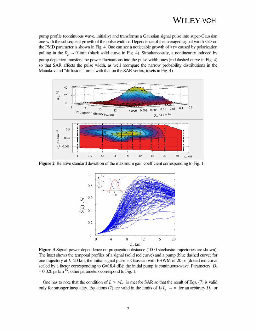
Figure 2 Relative standard deviation of the maximum gain coefficient corresponding to Fig. 1.
Figure 3 Signal power dependence on propagation distance (1000 stochastic trajectories are shown).
The inset shows the temporal profiles of a signal (solid red curve) and a pump (blue dashed curve) for
one trajectory at L=20 km; the initial signal pulse is Gaussian with FHWM of 20 ps (dotted red curve
scaled by a factor corresponding to G=18.4 dB); the initial pump is continuous-wave. Parameters: Dp
= 0.026 ps km-1/2
, other parameters correspond to Fig. 1.
One has to note that the condition of L > >Lc is met for SAR so that the result of Eqs. (7) is valid
only for stronger inequality. Equations (7) are valid in the limits of → ∞cL L for an arbitrary Dp or

8
→ 0pD for an arbitrary L or for both limits that mean the validity of a statement → ∞cL L and/or
→ 0pD for the Manakov limit described by Eqs. (7) (Fig. 5).
0.01 0.115
20
25
30
35
40
PD
F
PD
F
τ, p
s
Dp, ps km
-1/2
0
5
10
15
20
25
στ , %
20 25 30 35 400
10
20
PD
F
τ, ps
Dp=0.019 ps km
-1/2
30 35 400
20
40
τ, ps
Dp=0.0065 ps km
-1/2
20 25 300
20
40
τ, ps
Dp=0.16 ps km
-1/2
Figure 4. Dependences of the average signal pulse width <t> (black solid curve) and its relative
deviation st (red dashed curve) on the PMD parameter. Insets show the pulse width probability
distributions for Dp = 0.0065, 0.019, and 0.16 ps km-1/2
. Input signal pulse is Gaussian with the
FWHM of 20 ps and the peak power of 10 mW; L=20 km; signal and pump SOPs are collinear
initially.
5 10 15 20 25 30 35 40 45 500
5
10
15
20
<G
>,
dB
L, km
Figure 5 Dependence of the maximum <G> on fiber length L in the Manakov limit of Eqs. (8) (solid
curve), and for the exact model of Eqs. (1): Dp = 0.001 ps km-1/2
(circles) and 0.065 ps km-1/2
(triangles). Red and blue dashed curves correspond to the results obtained from Eqs. (7) for Dp =
0.001 ps km-1/2
and 0.065 ps km-1/2
, respectively. Signal and pump SOPs are collinear initially:
( )= =
1,0,0 .s p
With PMD growth, a deviation of an exact <G> (triangles, Fig. 5) from the Manakov limit (solid
curve) appears for fiber lengths near SAR ( 5 10L ≈ ÷ km). One has to note that the multi-scale
averaging technique, leading to Eqs. (6) (dashed curves in Fig. 5), provides an excellent approximation
to exact numerical results for both small and large PMDs at distances when depletion does not
contribute substantially. An important advance of this technique is that it describes statistical properties
such as gain relative standard deviation, relative signal gain, etc. [15]

9
When → ∞cL L and → 0pD , the relative standard deviation of the maximum gain coefficient
vanishes that corresponds to the domination of polarization pulling. The relative standard deviation of
gain is maximum in the region of SAR (Fig. 2), and the limit of large PMD and small fiber lengths is
characterized by decreasing but sufficiently large relative standard deviation of gain that results from
decorrelation of rapid relative rotations of pump-signal SOPs (i.e., their average relative projection
→ 0x ). <G> is minimal here and is defined by a “diffusion” limit (Fig. 5 for small L) [14].
Figure 6 Dependence of average minimal gain coefficient <G> on a fiber length L and a PMD
parameter Dp. Parameters correspond to Figure 1. Signal and pump SOPs are orthogonal initially:
( )= −
1,0,0s and ( )=
1,0,0p .
The case of minimal gain corresponding to initially orthogonal pump and signal SOPs (i.e.
( )= −
1,0,0s and ( )=
1,0,0p ) is illustrated in Figs. 6 and 7. One can see a threshold-like growth of
average gain with the growth of fiber length and PMD parameter. Such growth can be interpreted in
the terms of escape from a metastable state [16-18] of = −1x due to fluctuations of SOPs induced
by stochastic birefringence. Figure 7 demonstrates an extremal enhancement of such fluctuations in
the vicinity of threshold-growth of the average gain coefficient. Since the interaction length of signal-
pump SOPs increases with a fiber length, the polarization pulling increases, as well. As a result, the
average gain coefficient grows, and its fluctuations are suppressed. However, despite the case of Fig.
2, the relative standard deviation becomes maximal with minimization of PMD for a sufficiently large
L (Fig. 7). Such a shift of SAR into the region of smaller PMDs and larger fiber lengths can be
explained by the deceleration of SOP evolution to a polarization pulling state for the case of initially
orthogonal signal-pump SOPs with the decrease of Dp.
Figure 8 displays the PDG parameter. One can see the PDG suppression with increasing fiber
length and PMD parameter. The first tendency results from the enhancement of polarization pulling
with the growth of signal-pump SOPs interaction length. The second tendency results from the
intensive decorrelation of signal-pump SOPs with the decrease of beat length. Simultaneously, PDG
becomes extremely enhanced for small PMD in the vicinity of ≈ 10L km, which correlates with the
conjunction of SAR positions for minimal and maximal gains (see Figs. 2 and 7).

10
Figure 7 Relative standard deviation of the minimum gain coefficient corresponding to Figure 6.
As modern fiber Raman-based telecommunication systems support high-level signal powers (up to
100 mW) [19], it is of interest to consider the influence of input signal power on maximum gain and
its relative standard deviation. Though this value is beyond of the margins of the Eqs. (3, 4) validity,
the model based on Eqs. (3, 4) can be used for qualitative evaluation of the signal power influence on
the averaged gain and gain fluctuations. Figure 9 demonstrates the dependencies of <G> and σG on
the PMD parameter for different levels of ( )
0S . One can see a monotonic reduction of gain with
input signal power due to pump depletion. Such a reduction increases for small PMDs due to the effect
of polarization pulling, which causes more effective Raman amplification and, as a consequence, more
intensive pump depletion. Simultaneously, the relative standard deviation of gain decreases with the
( )
0S -growth, but the position of SAR does not change appreciably. One may assume that the
reduction of relative standard deviation with the signal power growth results from a stronger
polarization pulling which synchronizes the evolution of pump-signal SOPs.
Figure 8. PDG for the parameters corresponding to Figures 1, 6.

11
As was pointed out above, the gain noise caused by stochastic birefringence depends resonantly on
both PMD and propagation length. In real-world amplifiers, there are additional noise sources due to
the pump power and SOP fluctuations. Here, we consider the effect of pump power fluctuations on a
signal in relation to the PMD parameter and the fiber length. Figure 10 demonstrates the mean gain
standard deviations with (dashed curves) and without (solid curves) additive Gaussian pump noise.
One can see that stochastic birefringence dominates for large PMD, i.e. around the region of SAR.
Here, the integral pump-noise transfer function defined as
( )( )
( )σ σ∞
∞
= =
∫
∫
2 20int
0
10log 10logs
G P
p
RIN f dfH
RIN f df, (9)
(here σ P is the relative standard deviation for noisy pump and RINs,,p are the corresponding relative
intensity noises at frequency f [25]) takes the maximum value (dots connected by dotted curves in Fig.
10). The decrease of PMD reduces both σG and Hint, however, they do not vanish for the noisy pump
but tend to some constant value for Dp < <1 and L/Lc > >1. It is clear that the contribution of stochastic
birefringence is suppressed by polarization pulling in the →0pD limit so that only pump noise
contribution remains. Simultaneously, pump noise is suppressed by L-growth due to pump depletion
(see Fig. 3). However, such suppression becomes saturated with L-growth (Fig. 10) that is testified by
non-Gaussian statistics (Figs 11 and 12c, d).
The statistical properties of signal power without input pump noise are illustrated in Fig. 11. In the
diffusion limit, i.e. in the limit of large PMD, Raman amplification is almost polarization independent
due to fast relative rotation of pump and signal SOPs. As a result, the signal PDF close to Gaussian
and is narrow, but with a visible substructure due to residual polarization effects (Figure 11, a).
Approaching to SAR broadens PDF and enhances its visible substructure so that distribution becomes
rather “nonparametric” [26] (Fig. 11b). Transition to small PMD or/and large propagation distances
(Manakov limit) results in a non-Gaussian statistic which is close to “extreme value” one [27] with the
prolonged low power tail (Figures 11c, d). Figure 3 illustrates the corresponding contribution of low-
power stochastic trajectories. It is obvious that the cutting edge in this distribution is defined by
polarization pulling providing maximum gain. Nevertheless, some sustained fluctuations of the
relative SOPs around this state remain.
0.01 0.16
8
10
12
14
16
<G
>, d
B
Dp, ps km
-1/2
0
10
20
30
40
σG , %
Figure 9 Maximum gain <G> (solid curves) and its relative standard deviation
Gσ (dashed curves) for
different input signal powers: 20 mW (black), 50 mW (red) and 100 mW (blue). L=5 km, other
parameters correspond to Fig. 1.

12
Pump noise modifies the signal probability distributions, especially in the region of small PMD (Fig.
12). One can see from Figs. 12 (a,b), that the modifications are not substantial for the large PMD and
the relatively small propagation distances where the SAR contribution prevails. However, a Gaussian
input noise modifies distributions for small PMD or/and large L (see Figs. 12 (c,d)) so that they
become rather a Gaussian (or Burr-like in the case of (d)) than extreme one.
1E-3 0.01 0.10
10
20
30
40
σ G,
%
Dp, ps km
-1/2
5 km
10 km
20 km
40 km
0
10
20
30
Hin
t , dB
Figure 10. Dependencies of the relative standard deviation σG (solid and dashed curves concern the
noiseless and noisy pumps, respectively) and the integral pump-noise transfer function Hint (dots
connected by dotted curves) on the PMD parameter for different fiber lengths: 5 km (black), 10 km
(red), 20 km (blue), and 40 km (magenta). Pump power fluctuations are described by a Gaussian noise
with the standard deviation of 1%. Other parameters correspond to Figure 1.
Figure 11. Probability distributions of signal power for 1000 samples without pump noise. Dp = 0.16
(a), 0.026 (b,d), and 0.001 ps km-1/2
(c) and L=5 (a-c) and 40 km (d). Fitting curves correspond to
Gaussian distribution (red curves in (a), (b)), nonparametric distribution (blue curve in (b)), and

13
generalized extreme distribution (red curves in (c), (d)) obtained with the help of MATLAB statistics
toolbox. Other parameters correspond to Figure 1.
Figure 12 Probability distributions of signal power for 1000 samples with Gaussian pump noise. Dp
= 0.16 (a), 0.026 (b,d), and 0.001 ps/km-1/2
(c) and L=5 (a-c) and 40 km (d). Fitting curves
correspond to Gaussian distribution (red curves in (a), (b) and (c)), nonparametric distribution (blue
curve in (b)), and Burr distribution (red curve in (d)) obtained with the help of MATLAB statistics
toolbox. Other parameters correspond to Fig. 1.
4. Conclusion
Using direct stochastic simulation of coupled Manakov-PMD equations, we evaluate the contribution
of the stochastic anti-resonance phenomenon on fiber Raman amplifier gain, gain fluctuations and
pump-to-signal intensity noise transfer as a function of PMD parameter, fiber length and the signal
input power. We have found that although stochastic anti-resonance impact on the averaged gain and
the random birefringence-mediated gain fluctuations becomes negligible with increased length and
PMD parameter, it still contributes substantially to the pump-to-signal RIN transfer up to 10 dB for
FRA lengths over 40 km and Dp of 0.02 ps km-1/2
. In addition, the SAR leads to the pulse broadening
and emergence of the rare events taking the form of low output power pulses with the probability
heavily deviated from the Gaussian distribution. With the help of the separation of the deterministic
and stochastic evolution we have obtained a library of stochastic trajectories that allowed us to
substantially decrease computational time and required memory. This improvement in computational
efficiency can find potential applications in telecommunications for machine learning based
modulation format recognition [22], linear and nonlinear transmission impairments mitigation [23],
stochastic digital backpropagation [24] as well as in fiber lasers engineering for machine learning
based optimal laser parameters self-adjustment [25]. Comparison of the results of stochastic
simulations with the results for two analytical models has helped to determine the margins of the
analytical models as follows: (i) the model based on Eqs. (6) is using two-scale averaging and neglects

14
the pump depletion and so is valid for all PMD values, the small input signal powers (<1 mW) and
short fiber lengths of less than 6 km, (ii) the model based on Eqs. (7) is using single-scale averaging is
valid in the limit of the fiber lengths of L>25 km or small PMD values. The margins can help to justify
the application of the analytical models in the aforementioned limit cases to reduce substantially the
computational time required for machine learning based problems solving [22-25]. Including the
fluctuations of the pump SOP, pump-signal walk-off, group-delay dispersion and Kerr-nonlinearity
will introduce some corrections to signal-noise transfer for large fiber lengths but the analysis of these
effects is beyond the scope of the present article. Nevertheless, one has to note that Eqs. (5) admit a
straightforward generalization taking into account these effects that will be an object of our
forthcoming analysis.
Acknowledgements This work has been funded through grants FP7-PEOPLE-2012-IAPP (project
GRIFFON, No. 324391), Leverhulme Trust (Grant ref: RPG-2014-304), Spanish MINECO
TEC2015-71127-C2-1-R (project ANOMALOS), and Austrian Science Fund (FWF project P24916-
N27).
Received: ((will be filled in by the editorial staff))
Revised: ((will be filled in by the editorial staff))
Published online: ((will be filled in by the editorial staff))
Keywords: Stochastic processes, Nonlinear fiber optics, Polarization Phenomena, Fiber optic
amplifiers, Raman effect.
References
[1] P. K. A. Wai, C. R. Menyuk, IEEE J. Lightwave Technology 14, 148-157 (1996).
[2] C. R. Menyuk, J. Engineering Math. 36, 113-136 (1999)
[3] C. R. Menyuk, B. S. Marks, J Lightwave Technol. 24, 2806 (2006)
[4] G.P Agrawal, Nonlinear Fiber Optics (Academic Press, 2007).
[5] C. Headley & G.P. Agrawal (Eds.), Raman Amplification in Fiber Optical Communication
Systems (Amsterdam, Elsevier, 2005) p. 64.
[6] Q. Lin, G. P. Agrawal, J. Opt. Soc. Am. B 20, 1616-1631 (2003).
[7] V. V. Kozlov, J. Nuno, J. D. Ania-Castañón, and S. Wabnitz, Opt. Lett. 35, 3970-3972 (2010).
[8] V. V. Kozlov, J. Nuno, J. D. Ania-Castañón, and S. Wabnitz, IEEE J. Lightwave Technol. 29,
341-347 (2011).
[9] V. V. Kozlov, J. Nuno, J. D. Ania-Castañón, and S. Wabnitz, Opt. Lett. 37, 2073-2075 (2012).
[10] L. Ursini, S. Santagiustina, and L. Palmieri, IEEE Photon. Technol. Lett. 23, 254-256 (2011).
[11] M. Martinelli, M. Cirigliano, M. Ferrario, L. Marazzi, and P. Martelli, Opt. Express 17, 947-
955 (2009).
[12] S. Sergeyev, S. Popov, and A. T. Friberg, Optics Commun. 262, 114-119 (2006).
[13] S. Sergeyev, Opt. Express 19, 24268-24279 (2011).
[14] S. Sergeyev, S. Popov, and A. T. Friberg, IEEE J. Quantum Electron. QE-46, 1492-1497
(2010).
[15] V. Kalashnikov, S. V. Sergeyev, G. Jacobsen, S. Popov, and S. K. Turitsyn, Light: Science &
Applications 5, e16011 (2016).
[16] L. Gammaitoni, P. Hänggi, P. Jung, and F. Marchesoni, Rev. Mod. Phys. 70, 223 (1998)
[17] B. Lindner, J. Garsia-Ojalvo, A. Neiman, and L. Schimansky-Greif, Phys. Reports 392,
321-424 (2004).

15
[18] Th. Wellens, V. Shatochin, A. Buchleitner, Rep. Prog. Phys. 67, 45 (2004).
[19] D. I. Chang, W. Pelouch, P. Perrier, H. Fevrier, S. Ten, C. Towery, and S. Makovejs, Opt.
Express 22, 31057-31062 (2014).
[20] C. Martinelli, L. Lorcy, A. Durécu-Legrand, D. Mongardien, S. Borne, IEEE J. Lightwave
Technol. 24, 3490-3496 (2006).
[21] J. Cheng, M. Tang, A. P. Lau, C. Lu, L. Wang, Z. Dong, S. M. Bilal, S. Fu, P. P. Shum, D.
Liu, Opt. Express 23, 11838-11854 (2015).
[22] R. Boada, R. Borkowski, and I. T. Monroy, Opt. express 23, 15521-15531 (2015).
[23] D. Zibar, L.H.H. de Carvalho, M. Piels, A. Doberstein, J. Diniz, B. Nebendahl, C.
Franciscangelis, J. Estaran, H. Haisch, N.G. Gonzalez, and J.C.R. de Oliveira, IEEE J.
Lightwave Technol. 33, 1333-1343 (2015).
[24] N. V. Irukulapati, H. Wymeersch, P. Johannisson, and E. Agrell, IEEE Trans. Commun. 62,
3956-3968 (2014).
[25] X. Fu, S. L. Brunton, and J. N. Kutz, Opt. express, 22, 8585-8597 (2014).
[26] L. Wasserman, All of Nonparametric Statistics (NY, Springer, 2006).
[27] S. Coles, An Introduction to Statistical Modeling of Extreme Values (London, Springer,
2001).

16
Supporting Information
Stochastic phenomena in a fiber Raman amplifier
Vladimir Kalashnikov1,5
, Sergey V. Sergeyev1,*
, Juan Diego Ania-Castanón2,
Gunnar Jacobsen3 and Sergei Popov
4
*Corresponding Author: [email protected]
1Aston Institute of Photonic Technologies, Aston University, Aston Triangle, Birmingham,
B4 7ET, UK 2 Instituto de Optica CSIC, Serrano 121, Madrid, 28006, Spain
3Acreo, Electrum 236, SE-16440, Kista, Sweden
4Royal Institute of Technology (KTH), SE-1640, Stockholm, Sweden
5Institute of Photonics, Vienna University of Technology, Gusshausstr. 27/387, Vienna, A-
1040, Austria
This document provides supporting information to “Stochastic phenomena in a fiber
Raman amplifier.” We describe numerical and averaging techniques underlying our
results.
1. Numerical technique
The structure of Eqs. (4,5) allows splitting the numerical simulations into two independent
parts notably i) independent solution of a system of stochastic ordinary differential equations
(SDE) (4) that gives a “library” of stochastic material parameters for ii) simulation of field
evolution (in Jones representation) based on Eqs. (5) with independent stochastic coefficients.
One has to note that Eqs. (5) can be generalized with taking into account group-delay, group-
delay dispersion, and Kerr nonlinearity so that the resulting model becomes a split system of
SDE + “nonlinear partial differential equations with independent stochastic coefficients.” As
the solution of SDE is most challenging task, a careful choice of numerical technique is
required. The algorithm convergence can be controlled by following property of the unitary T-
matrix:
( ) ( ) ( ) ( )+ = = =2 2
1 2 1 21, 0 1, 0 0,t z t z t t (ES1)
and unitarity has to persist during evolution by virtue of unitarity of Σ. Figure S1 shows a
behavior of invariant (ES1) calculated with the help of Wolfram Mathematica 10.0 using
StratanovichProcess and RandomFunction procedures, and four different methods: “Milstein”
and “Stochastic Runge-Kutta” (Figure S1, (1)), as well as “Stochastic Runge-Kutta Scalar
Noise” and “Kloeden-Platen-Schurz” (Figure S1, (2)). One can see that last two algorithms
preserve (ES1), and they were used in our simulations.
To accelerate calculations substantially, we used MATLAB. In this case, the fast and good
convergence was provided by the Weak Order 2 Stochastic Runge-Kutta Method [1]:

17
Y0
= X0
,
U =Yn
+ A Yn( )δ +B Y
n( )∆Wn
,
U± =Yn
+ A Yn( )δ ±B Y
n( ) δ ,
Yn+1
=Yn
+ δ2A U( )+ A Y
n( )
+
∆Wn
4B U+( )+B U−( ) +2B Y
n( )
+
+∆W
n( )2
−δ
4 δB U+( )−B U−( )
, (ES2)
where the Stratonovich type SDE is expressed formally in the form of
( ) ( ) ( ) ( ), ,X z A z X dz B z X dW z= + . (ES3)
In Eqs. (ES2), ( ) ( )δ + += − ∆ = −1 1,n n n nz z W W z W z , W(z) is a Wiener process, and X, A, B
can be multi-component.
Figure S1. Evolution of ( ) ( )+2 2
1 2t z t z -invariant from Eq. (4) simulated by the Milstein
and Stochastic Runge-Kutta (1) as well as the Stochastic Runge-Kutta Scalar Noise and
Kloeden-Platen-Schutz (2) algorithms.
2. Averaging technique and Manakov limit
Let us express in Eq. (5) in the following form:
σ
= − ɶ
*1 4
3
4 1
,X X
X X (ES4)
where a new six-component vector X is introduced:

18
X1
= t1
2− t
2
2, X
2= − t
1t
2+t
1
*t2
*( ) , X3
= i t1t
2−t
1
*t2
*( ) ,
X4
= 2it1t
2
* , X5
= t1
2 −t2
*2 , X6
= −i t1
2 +t2
*2( ) ,
(ES5)
which obeys to SDE (ES3) with
( ) ( )( ) ( )
= − −
= − −
3 2 6 5
2 1 5 4
0, 2 ,2 ,0, 2 ,2 ,
2 , 2 ,0,2 , 2 ,0 .
T
p p p p
T
A X b X b X b X b X
B X X X X X
(ES6)
Splitting of the initial system (2) into the stochastic material and field parts simplifies an
averaging over the stochastic birefringence [2]. Applying the Dunkin formula and the
Stratonovich generator Γ [3-5]:
( ) ( )
= = =
Ω = Γ
∂∂ ∂Γ = + + ∂ ∂ ∂ ∑ ∑∑
6 6 6
1 1 1
ˆ ,
1ˆ2
i
k
kk k l l
k k lk c l k
d ff X
dz
BA B B B
X L X X
(ES7)
(f is some function of X) results in the following groups of equations for averaged ( )f X :
(ES8)
d X1
2
dz= 4σ 2 X
2
2 − X1
2( ) ,
d X2
2
dz= 4σ 2 X
1
2 − X2
2( )−4bpX
2X
3,
d X3
2
dz= 4b
pX
2X
3,
d X2X
3
dz=2b
pX
2
2 − X3
2( )−2σ 2 X2X
3,
X1
2 , X2
2 , X3
2 , X2X
3( )z=0
= 1,0,0,0( ). (ES9)
d X1
dz= −2σ 2 X
1, d X
2
dz= −2b
pX
3−2σ 2 X
2,
d X3
dz=2b
pX
2, d X
4
dz= −2σ 2 X
4,
d X5
dz= −2b
pX
6−2σ 2 X
5, d X
6
dz= 2b
pX
5,
X1
, X2
, X3
, X4
, X5
, X6( )
z=0
= 1,0,0,0,0,0( ).

19
d X4
2
dz= 4σ 2 X
5
2 − X4
2( ) ,
d X5
2
dz= 4σ 2 X
4
2 − X5
2( ) −4bpX
5X
6,
d X6
2
dz= 4b
pX
5X
6,
d X5X
6
dz= 2b
pX
5
2 − X6
2( ) −2σ 2 X5X
6,
X4
2 , X5
2 , X6
2 , X5X
6( )z=0
= 0,1,−1,−i( ). (ES10)
d X4
2
dz= 4σ 2
X5
2− X
4
2
,
d X5
2
dz= 4σ 2 X
4
2− X
5
2
−2b
pX
5X
6
* + X6X
5
*( ) ,
d
dzX
5X
6
* + X6X
5
*( ) =
= 4bp
X5
2− X
6
2
−2σ 2 X
5X
6
* + X6X
5
*( ) ,
X4
2, X
5
2, X
5X
6
* , X5X
6
* + X6X
5
*
z=0
= 0,1,1,0( ). (ES11)
d X3X
6
dz= 2b
pX
2X
6+ X
3X
5( ) ,
d X2X
5
dz= −2b
pX
2X
6+ X
3X
5( )−4σ 2X
2X
5− X
1X
4( ) ,
d X1X
4
dz= 4σ 2
X2X
5− X
1X
4( ) ,
d
dzX
2X
6+ X
3X
5( ) =
= 4bp
X2X
5− X
3X
6( )−2σ 2 X2X
6+ X
3X
5( ) ,
X3X
6, X
2X
6+ X
3X
5, X
2X
5, X
1X
4( )z=0
= 0,0,0,0( ).
(ES12)

20
d X3X
6
*
dz= 2b
pX
2X
6
* + X3X
5
*( ) ,
d X2X
6
*
dz= 2b
pX
2X
5
* − X3X
6
*( )−2σ 2 X2X
6
* ,
d X2X
5
*
dz= −2b
pX
2X
6
* + X3X
5
*( )−4σ 2 X2X
5
* − X1X
4
*( ) ,
d X1X
4
*
dz= 4σ 2 X
2X
5
* − X1X
4
*( ) ,
d X3X
5
*
dz= 2b
pX
2X
5
* − X3X
6
*( )−2σ 2 X3X
5
* ,
X3X
6
* , X2X
6
* , X2X
5
* , X1X
4
* , X3X
5
*( )z=0
= 0,0,0,0,0( ). (ES13)
A group of Eqs. (ES8) has a trivial solution ( )σ= − 21 exp 2X z which leads to the “Manakov
limit” equations (8) in the Stokes representation.
3. Pump depletion and signal/pulse temporal profiles
The real-world signal in Eqs. (4) is a pulse (i.e., t-dependent) whereas pump is initially
continuous-wave (CW, i.e. t-independent). Eqs. (4) allow the direct extension of
dimensionality including the t-coordinate [6]:
(ES14)
where group-delay are defined by β λ π=, , , 2 .s p s p s pb c
It is clear that pump depletion will modify both pump and signal profiles during evolution so
that a passive (nonlinear) negative feedback appears. Such a feedback causes the signal pulse
broadening, flattens pulse shape, and creates a gap in the pump CW-profile (Figure S2).

21
Figure S2. Signal (left) and pump (right) profiles along one stochastic trajectory for Dp=0.01
ps2 km
-1/2. Initial signal pulse is Gaussian with 20 ps FWHM and 10 mW peak power; the
initial pump is CW with 1 W power. The group-delays are not included.
Figure S2 presents an evolution along one stochastic trajectory of (ES14) defined by σɶ3 . The
signals at L=20 km for six different trajectories are shown in Figure S3 for the same
parameters. One can see that the pulse profile can become nontrivial due to the coupling of
different polarization components.
Calculations suggest that impact of group-delay for L=20 km and the initial pulse width of
even 5 ps is negligible.
Figure S3. Final (L=20 km) signal profiles corresponding to six stochastic trajectories for
Dp=0.01 ps2 km
-1/2. Initial signal pulse is Gaussian with 20 ps FWHM and 10 mW peak
power; the initial pump is CW with 1 W power. The group-delays are not included.
The relevant Mathematica and MATLAB codes, as well as the library of pre-calculated
stochastic trajectories for (ES14) can be found in [7].
REFERENCES
[1] B. Riadh, H. Querdiane, Int. J. Math. Analysis 8, 229 (2014).
[2] D. Marcuse, C. R. Menyuk, P. K. A. Wai, IEEE J. Lightwave Technology 15, 1735 (1997).
[3] L. Arnold. Stochastic Differential Equations: Theory and Applications (NY, Wiley, 1974).
[4] B. ∅ksendal. Stochastic Differential Equations (Berlin, Springer, 2007).
[5] G. A. Pavliotis. Stochastic Processes and Applications: Diffusion Process, the Fokker-Planck
and Langevin Equations (NY, Springer, 2014).
[6] V. L. Kalashnikov, S. V. Sergeyev, Stochastic Anti-Resonance in Polarization Phenomena, in
The Foundations of Chaos Revisited: From Poincaré to Recent Advancements (Springer,
2016), 159-179.

22
[7] V. L. Kalashnikov, Stochastic Anti-Resonance in a Fibre Raman Amplifier, web-resource:
http://info.tuwien.ac.at/kalashnikov/programs.html