Embed Size (px)
Citation preview
Stochastic p-Robust Location Problems
Lawrence V. Snyder∗
Department of Industrial and Systems Engineering
Lehigh University
200 West Packer Avenue, Mohler Lab
Bethlehem, PA, 18015
Mark S. DaskinDepartment of Industrial Engineering and Management Sciences
Northwestern University
2145 Sheridan Road
Evanston, IL, 60208
November 7, 2005Final version published in IIE Transactions 38(11), 971–985, 2006
Abstract
The two most widely considered measures for optimization under uncertainty are
minimizing expected cost and minimizing worst-case cost or regret. In this paper, we
present a new robustness measure that combines the two objectives by minimizing the
expected cost while bounding the relative regret in each scenario. In particular, the
models seek the minimum-expected-cost solution that is p-robust; i.e., whose relative
regret is no more than 100p% in each scenario. We present p-robust models based
on two classical facility location problems. We solve both problems using variable
splitting, with the Lagrangian subproblem reducing to the multiple-choice knapsack
problem. For many instances of the problems, finding a feasible solution, and even
determining whether the instance is feasible, is difficult; we discuss a mechanism for
determining infeasibility. We also show how the algorithm can be used as a heuristic
to solve minimax-regret versions of the location problems.
∗Corresponding author.
1

Keywords: robust facility location, stochastic p-robustness, variable splitting, multiple-
choice knapsack problem
2
1 Introduction
Optimization under uncertainty typically employs one of two approaches, stochastic
optimization or robust optimization. In stochastic optimization, random parameters
are governed by a probability distribution, and the objective is to find a solution that
minimizes the expected cost. In robust optimization, probabilities are not known, and
uncertain parameters are specified either by discrete scenarios or by continuous ranges;
the objective is to minimize the worst-case cost or regret. (Though these approaches
are the most common, many other approaches have been proposed for both stochastic
and robust optimization; for a review of their application to facility location problems,
see Owen and Daskin (1998) or Snyder (2005a).) The former approach finds solutions
that perform well in the long run on average, with poor performance at some times
balanced by good performance at others. However, many decision makers are evaluated
ex post, after the uncertainty has been resolved and costs have been realized; in such
situations, decision makers are often motivated to seek minimax regret solutions that
appear effective no matter which scenario is realized. On the other hand, minimax
objectives tend to be overly pessimistic, planning against a scenario that, while it may
be disastrous, is unlikely to occur.
In this paper, we discuss facility location models that combine the advantages
of both the stochastic and robust optimization approaches by seeking the least-cost
solution (in the expected value) that is p-robust; i.e., whose relative regret in each
scenario is no more than p, for given p ≥ 0. This robustness measure will be referred to
as stochastic p-robustness. The standard min-expected-cost objective can be obtained
by setting p = ∞. The resulting solution is optimal in the stochastic optimization sense
but may perform poorly in certain scenarios. By successively reducing p, one obtains
solutions with smaller maximum regret but greater expected cost. One objective of
this paper is to demonstrate empirically that substantial improvements in robustness
can be attained without large increases in expected cost.
We consider two classical facility location problems, the k-median problem (kMP)
and the uncapacitated fixed-charge location problem (UFLP). The problems we for-
mulate will be referred to as the stochastic p-robust kMP (p-SkMP) and the stochastic
p-robust UFLP (p-SUFLP), respectively. Both customer demands and transportation
3
costs may be uncertain; the possible values of the parameters are specified by discrete
scenarios, each of which has a specific probability of occurrence. The p-SkMP and
p-SUFLP are two-stage models, in that strategic decisions (facility location) must be
made now, before it is known which scenario will come to pass, while tactical decisions
(assignment of retailers to DCs) are made in the future, after the uncertainty has been
resolved. However, by simply multiplying the results by the number of time periods
in the planning horizon, one can think of these as multi-period models in which we
make strategic decisions now and then make separate tactical decisions in each time
period. Thus our models can accommodate parameters that are not time stationary.
If we make decisions now that hedge poorly against the various scenarios, we must live
with the consequences as parameters change.
We solve both problems using a variable-splitting (or Lagrangian decomposition)
formulation whose subproblems reduce to instances of the multiple-choice knapsack
problem (MCKP), a variant of the classical knapsack problem. Feasible solutions are
found using a simple upper-bounding heuristic. For small values of p, it may be difficult
to find a feasible solution, or even to determine whether the problem is feasible. We
provide an upper bound that is valid for any feasible solution and use this bound to
provide a mechanism for detecting infeasibility early in the algorithm’s execution. By
solving the problem iteratively with multiple values of p, one can solve minimax-regret
versions of the kMP and UFLP. Since our algorithm cannot determine the feasibility
of every problem within a given time or iteration limit, this method is a heuristic.
This paper makes the following contributions to the literature. First, we introduce a
new measure for optimization under uncertainty (stochastic p-robustness) that requires
a given level of performance in each scenario while also minimizing the expected cost.
Second, we formulate and solve stochastic p-robust versions of the kMP and UFLP.
Our solution method is based on well-known methods, but the use of the MCKP in
the Lagrangian subproblems is novel, as is the infeasibility test. Third, we provide a
heuristic for solving minimax-regret versions of the kMP and UFLP; to date, these
problems have been solved optimally for special instances (e.g., on tree networks)
but only heuristically in the more general case. Our heuristic has the advantages
of providing both upper and lower bounds on the optimal minimax regret value and of
guaranteeing a given level of accuracy, though execution times may be long for small
4
optimality tolerances.
The remainder of this paper is structured as follows. In Section 2, we formally
define stochastic p-robustness and review the relevant literature. We formulate the
p-SkMP and present a variable-splitting algorithm for it in Section 3 and do the same
for the p-SUFLP in Section 4. In Section 5, we discuss a mechanism for detecting
infeasibility. The minimax-regret heuristic is presented in Section 6. Section 7 contains
computational results, and Section 8 contains our conclusions.
2 Preliminaries and Literature Review
The k-median problem (kMP; Hakimi 1964, 1965) and the uncapacitated fixed-charge
location problem (UFLP; Balinski 1965) are classical facility location problems; for a
textbook treatment see Daskin (1995). Sheppard (1974) was one of the first authors
to propose a scenario approach to facility location, in 1974. He suggests selecting
facility locations to minimize the expected cost, though he does not discuss the issue
at length. Since then, the literature on facility location under uncertainty has become
substantial; we provide only a brief overview here and refer the reader to other sources
(Brandeau and Chiu 1989, Current, Daskin and Schilling 2002, Louveaux 1993, Owen
and Daskin 1998, Snyder 2005a) for more detailed reviews.
Weaver and Church (1983) present a Lagrangian relaxation algorithm for a stochas-
tic version of the kMP that is equivalent to our model with p set to ∞. Their ba-
sic strategy is to treat the problem as a deterministic problem with |I||S| customers
instead of |I| (where I is the set of customers and S is the set of scenarios) and
then to apply a standard Lagrangian relaxation method for it (Cornuejols, Fisher and
Nemhauser 1977, Geoffrion 1974). Mirchandani, Oudjit and Wong (1985) begin with
the same formulation as Weaver and Church (1983), explicitly reformulating it as a
deterministic kMP with |I||S| customers. They also suggest a Lagrangian relaxation
method, but they relax a different constraint to attain a problem that is equivalent to
the UFLP. Their method provides tight bounds and requires only a small number of
iterations, though each iteration is computationally expensive.
The two most common measures of robustness that have been applied to facility
location problems in the literature are minimax cost (minimize the maximum cost
5
across scenarios) and minimax regret (minimize maximum regret across scenarios).
The regret of a solution in a given scenario is the difference between the cost of the
solution in that scenario and the cost of the optimal solution for that scenario. Robust
optimization problems tend to be more difficult to solve than stochastic optimization
problems because of their minimax structure. As a result, research on robust facility
location generally falls into one of two categories: optimal (often polynomial-time) al-
gorithms for restricted problems like 1-median problems or k-medians on tree networks
(Averbakh and Berman 2000, Burkard and Dollani 2001, Chen and Lin 1998, Vairak-
tarakis and Kouvelis 1999), or heuristics for more general problems (Current, Ratick
and ReVelle 1997, Serra, Ratick and ReVelle 1996, Serra and Marianov 1998).
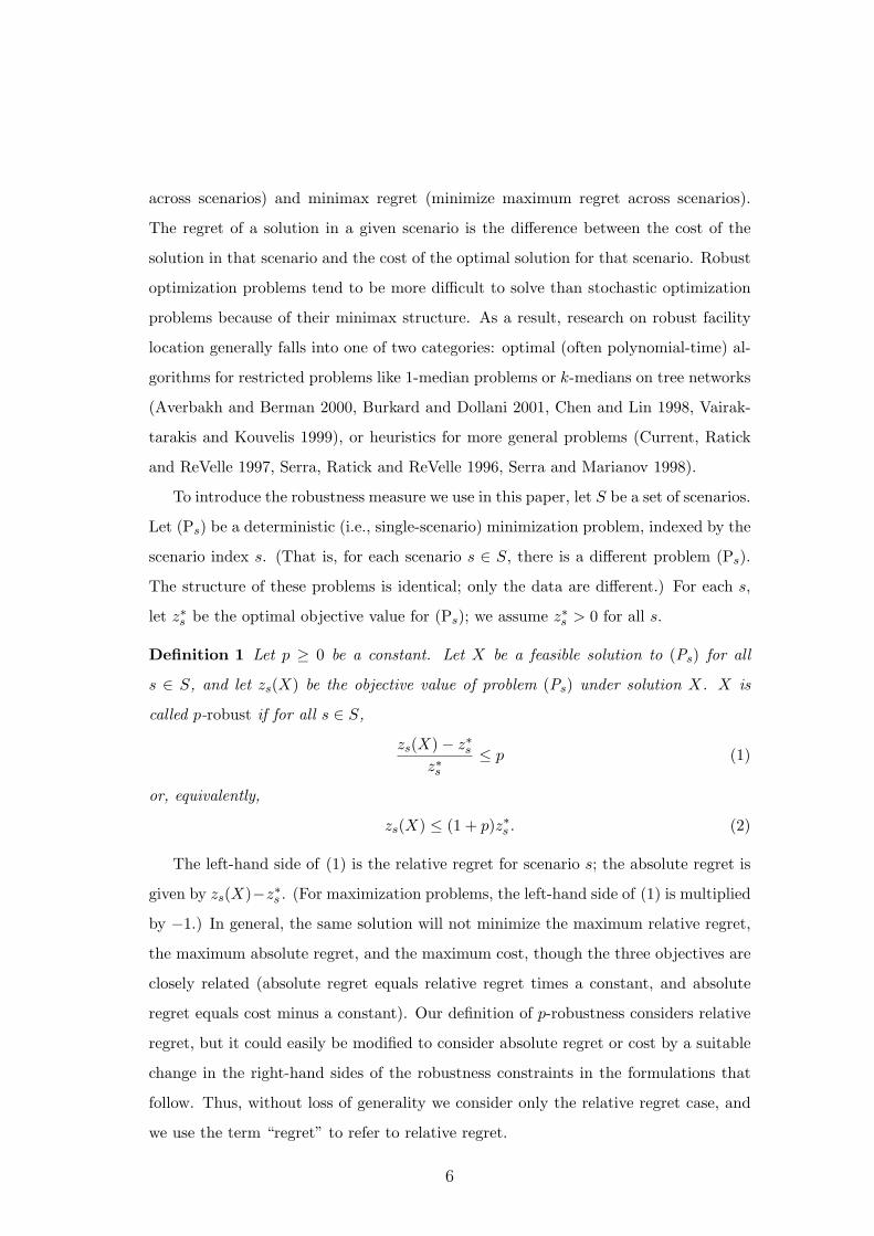
To introduce the robustness measure we use in this paper, let S be a set of scenarios.
Let (Ps) be a deterministic (i.e., single-scenario) minimization problem, indexed by the
scenario index s. (That is, for each scenario s ∈ S, there is a different problem (Ps).
The structure of these problems is identical; only the data are different.) For each s,
let z∗s be the optimal objective value for (Ps); we assume z∗s > 0 for all s.
Definition 1 Let p ≥ 0 be a constant. Let X be a feasible solution to (Ps) for all
s ∈ S, and let zs(X) be the objective value of problem (Ps) under solution X. X is
called p-robust if for all s ∈ S,
zs(X)− z∗sz∗s
≤ p (1)
or, equivalently,
zs(X) ≤ (1 + p)z∗s . (2)
The left-hand side of (1) is the relative regret for scenario s; the absolute regret is
given by zs(X)−z∗s . (For maximization problems, the left-hand side of (1) is multiplied
by −1.) In general, the same solution will not minimize the maximum relative regret,
the maximum absolute regret, and the maximum cost, though the three objectives are
closely related (absolute regret equals relative regret times a constant, and absolute
regret equals cost minus a constant). Our definition of p-robustness considers relative
regret, but it could easily be modified to consider absolute regret or cost by a suitable
change in the right-hand sides of the robustness constraints in the formulations that
follow. Thus, without loss of generality we consider only the relative regret case, and
we use the term “regret” to refer to relative regret.
6

The notion of p-robustness was first introduced in the context of facility layout
(Kouvelis, Kurawarwala and Gutierrez 1992) and used subsequently in the context of
an international sourcing problem (Gutierrez and Kouvelis 1995) and a network design
problem (Gutierrez, Kouvelis and Kurawarwala 1996). All three problems are also
discussed in Kouvelis and Yu’s (1997) book on robust optimization. These papers do
not refer to this robustness measure as p-robustness, but simply as “robustness.” We
will adopt the term “p-robust” to distinguish this robustness measure from others. The
international sourcing paper (Gutierrez and Kouvelis 1995) presents an algorithm that,
for a given p and N , returns either all p-robust solutions (if there are fewer than N of
them) or the N solutions with smallest maximum regret. The sourcing problem reduces
to the UFLP, so the authors are essentially solving a p-robust version of the UFLP,
but unfortunately their algorithm contains an error that makes it return incomplete,
and in some cases incorrect, results (Snyder 2005b).
It is sometimes convenient to specify a different regret limit ps for each scenario
s—for example, to allow low-probability scenarios to have larger regrets. In this case,
one simply replaces p with ps in (1) and (2). Denoting by p the vector (p1, . . . , p|S|),
we say a solution is p-robust if the modified inequalities hold for all s. For the sake of
convenience, we will assume throughout this paper that ps = p for all s ∈ S, though
all of our results can easily be extended to the more general case.
The p-robustness measure can be combined with a min-expected-cost objective
function to obtain problems of the following form:
minimize∑
s∈S
qszs(X)
subject to zs(X) ≤ (1 + p)z∗s ∀s ∈ S
X ∈ X
where qs is the probability that scenario s occurs and X is the set of solutions that are
feasible for all (Ps). We call the resulting robustness measure stochastic p-robustness.
3 The p-SkMP
In this section, we formulate the stochastic p-robust k-median problem (p-SkMP) and
then present a variable-splitting algorithm for it.
7
3.1 Notation
We define the following notation:
Sets
I = set of customers, indexed by i
J = set of potential facility sites, indexed by j
S = set of scenarios, indexed by s
Parameters
his = demand of customer i under scenario s
dijs = cost to transport one unit from facility j to customer i under scenarios s
p = desired robustness level, p ≥ 0
z∗s = optimal objective value of the kMP under the data from scenario s
qs = probability that scenario s occurs
k = number of facilities to locate
Decision Variables
Xj = 1 if facility j is opened, 0 otherwise
Yijs = 1 if facility j serves customer i in scenario s, 0 otherwise
The robustness coefficient p is the maximum allowable regret. The regret is com-
puted using z∗s , which is an input to the model; the z∗s values are assumed to have
been computed already by solving |S| separate (deterministic) PMPs. Such problems
can be solved to optimality using a variety of well-known techniques, including La-
grangian relaxation embedded in branch and bound (Daskin 1995, 2004). Note that
the assignment variables (Y ) are dependent on s while the location variables (X) are
not, reflecting the two-stage nature of the problem.
3.2 Formulation
The p-SkMP is formulated as follows:
(p-SkMP) minimize∑
s∈S
∑
i∈I
∑
j∈J
qshisdijsYijs (3)
8
subject to∑
j∈J
Yijs = 1 ∀i ∈ I,∀s ∈ S (4)
Yijs ≤ Xj ∀i ∈ I,∀j ∈ J,∀s ∈ S (5)∑
i∈I
∑
j∈J
hisdijsYijs ≤ (1 + p)z∗s ∀s ∈ S (6)
∑
j∈J
Xj = k (7)
Xj ∈ {0, 1} ∀j ∈ J (8)
Yijs ∈ {0, 1} ∀i ∈ I,∀j ∈ J,∀s ∈ S (9)
The objective function (3) minimizes the expected transportation cost over all sce-
narios. Constraints (4) ensure that each customer is assigned to a facility in each
scenario. Constraints (5) stipulate that these assignments be to open facilities. Con-
straints (6) enforce the p-robustness condition, while (7) states that k facilities are to
be located. Constraints (8) and (9) are standard integrality constraints. Note that,
as in the classical kMP, the optimal Y values will be integer even if the integrality
constraints (9) are non-negativity constraints. We retain the integrality constraints
both to emphasize the binary nature of these variables and because the subproblems
formulated below do not have the integrality property; requiring the Y variables to be
binary therefore tightens the relaxation.
If p = ∞, this formulation is equivalent to the model studied by Mirchandani et al.
(1985) and Weaver and Church (1983) since constraints (6) become inactive.
3.3 Complexity
Proposition 1 below says that the p-SkMP is NP-hard; this should not be surprising
since it is an extension of the kMP, which is itself NP-hard (Garey and Johnson 1979).
What may be surprising, however, is that the feasibility problem—determining whether
a given instance of the p-SkMP is feasible—is NP-complete. This is not true of either
the kMP or its usual stochastic or robust extensions (finding a min-expected-cost or
minimax-regret solution, respectively), since any feasible solution for the kMP is also
feasible for these extensions. Similarly, the feasibility question is easy for the capaci-
tated kMP since it can be answered by determining whether the sum of the capacities
of the k largest facilities exceeds the total demand. One would like some mechanism
9
for answering the feasibility question for the p-SkMP in practice to avoid spending too
much time attempting to solve an infeasible instance. This issue is discussed further
in Section 5.
Proposition 1 The p-SkMP is NP-hard.
Proof. If |S| = 1 and p = ∞, the p-SkMP reduces to the classical kMP, which is
NP-hard.
Proposition 2 For |S| ≥ 2, the feasibility problem for the p-SkMP is NP-complete.
Proof. First, the feasibility problem is in NP since the feasibility of a given solution
can be checked in polynomial time. To prove NP-completeness, we reduce the 0–1
knapsack problem to p-SkMP; the 0–1 knapsack problem is NP-complete (Garey and
Johnson 1979). Let the knapsack instance be given by
(KP) maximizen∑
k=1
akZk
subject ton∑
k=1
bkZk ≤ B
Zk ∈ {0, 1} ∀k = 1, . . . , n
The decision question is whether there exists a feasible Z such that
n∑
k=1
akZk ≥ A. (10)
We can assume WLOG that∑n
k=1 ak ≥ A, otherwise the problem is clearly infeasible.
We create an equivalent instance of the p-SkMP as follows. Let I = J = {1, . . . , 2n}and S = {1, 2}. Transportation costs are given by
cijs =
1, if j = i± n
∞, otherwise(11)
for all i, j = 1, . . . , 2n and s = 1, 2. Demands are given by
(hi1, hi2) =
(ai + ε, ε), if 1 ≤ i ≤ n
(ε, biAB + ε), if n + 1 ≤ i ≤ 2n
(12)
10

where 0 < ε < min {mink=1,...,n{ak}, mink=1,...,n{bk}} and A =∑n
k=1 ak−A. Let k = n
and p = A/z∗1 .
The resulting instance is pictured in Figure 1. The optimal solution in scenario 1
is to set X1 = . . . = Xn = 1 and Xn+1 = . . . = X2n = 0, with a total cost of z∗1 = nε.
Similarly, the optimal cost in scenario 2 is z∗2 = nε. We prove that the p-SkMP instance
is feasible if and only if the knapsack instance has a feasible solution for which (10)
holds; therefore, the polynomial answerability of the feasibility question for the p-SkMP
implies that of the decision question posed for the 0–1 knapsack problem.
[Insert Figure 1 here.]
(⇒) Suppose that the given instance of the p-SkMP is feasible, and let (X,Y ) be a
feasible solution. Clearly Xi + Xi+n = 1 for all i = 1, . . . , n since the cost of serving i
or i + n from a facility other than i or i + n is prohibitive. Let
Zk =
1, if Xk = 1
0, if Xk+n = 1(13)
for k = 1, . . . , n. Since (X,Y ) is feasible, it satisfies constraint (6) for scenario 1,
namely
2n∑
i=1
2n∑
j=1
hi1cij1Yij1 ≤ (1 + p)z∗1
=⇒∑
i:Xi+n=1
(ai + ε) +∑
i:Xi=1
ε ≤ A + z∗1
=⇒∑
i:Xi+n=1
ai + nε ≤n∑
k=1
ak −A + nε
=⇒n∑
k=1
ak(1− Zk) ≤n∑
k=1
ak −A
=⇒n∑
k=1
akZk ≥ A
(14)
11
In addition, (X, Y ) satisfies constraint (6) for scenario 2:
2n∑
i=1
2n∑
j=1
hi2cij2Yij2 ≤ (1 + p)z∗2
=⇒∑
i:Xi=1
(bi
A
B+ ε
)+
∑
i:Xi+n=1
ε ≤ A + z∗2
=⇒∑
i:Xi=1
bkA
B+ nε ≤ A + nε
=⇒n∑
k=1
bkA
BZk ≤ A
=⇒n∑
k=1
bkZk ≤ B
(15)
Therefore the knapsack instance is satisfied; i.e., there exists a feasible Z whose objec-
tive function is greater than or equal to A.
(⇐) Now suppose that Z is a feasible solution to the knapsack instance that satisfies
(10). Define a solution to the p-SkMP by
Xi =
1, if Zi = 1
0, if Zi = 0
Xi+n = 1−Xi
for k = 1, . . . , n, and
Yijs =
1, if 1 ≤ i ≤ n, j ∈ {i, i + n}, and Xj = 1
1, if n + 1 ≤ i ≤ 2n, j ∈ {i, i− n}, and Xj = 1
0, otherwise
for i, j = 1, . . . , 2n, s = 1, 2.
Clearly (X,Y ) satisfies constraints (4), (5), and (7)–(9). The feasibility of (X, Y )
with respect to (6) follows from reversing the implications in (14) and (15). Therefore
the p-SkMP instance is feasible, completing the proof.
Note that Proposition 2 only applies to problems in which |S| ≥ 2. If |S| = 1, then
for p ≥ 0 the problem is trivially feasible by definition since the left-hand side of (6)
is the kMP objective function and the right-hand side is greater than or equal to its
optimal objective value.
12

3.4 Variable-Splitting Algorithm
3.4.1 Model Reformulation
If p = ∞, constraints (6) are inactive and the p-SkMP can be solved by relaxing
constraints (4); Weaver and Church (1983) show that the resulting subproblem is easy
to solve since it separates by j and s. But when p < ∞, the subproblem obtained using
this method is not separable since constraints (6) tie the facilities j together. Instead,
we propose an algorithm based on variable splitting.
Variable splitting, also known as Lagrangian decomposition, is used by Barcelo, Fer-
nandez and Jornsten (1991) to solve the capacitated facility location problem (CFLP).
The method involves the introduction of a new set of variables to mirror variables
already in the model, then forcing the two sets of variables to equal each other via a
new set of constraints. These constraints are then relaxed using Lagrangian relaxation
to obtain two separate subproblems. Each set of constraints in the original model is
written using one set of variables or the other to obtain a particular split. The bound
from variable splitting is at least as tight as that from traditional Lagrangian relaxation
and is strictly tighter if neither subproblem has the integrality property (Cornuejols,
Sridharan and Thizy 1991, Guignard and Kim 1987). In our case, another attraction of
variable splitting is that straightforward Lagrangian relaxation does not yield separable
subproblems.
The variable-splitting formulation of (p-SkMP) is obtained by introducing a new set
of variables W and setting them equal to the Y variables using a new set of constraints:
(p-SkMP-VS) minimize β∑
s∈S
∑
i∈I
∑
j∈J
qshisdijsYijs
+(1− β)∑
s∈S
∑
i∈I
∑
j∈J
qshisdijsWijs (16)
13
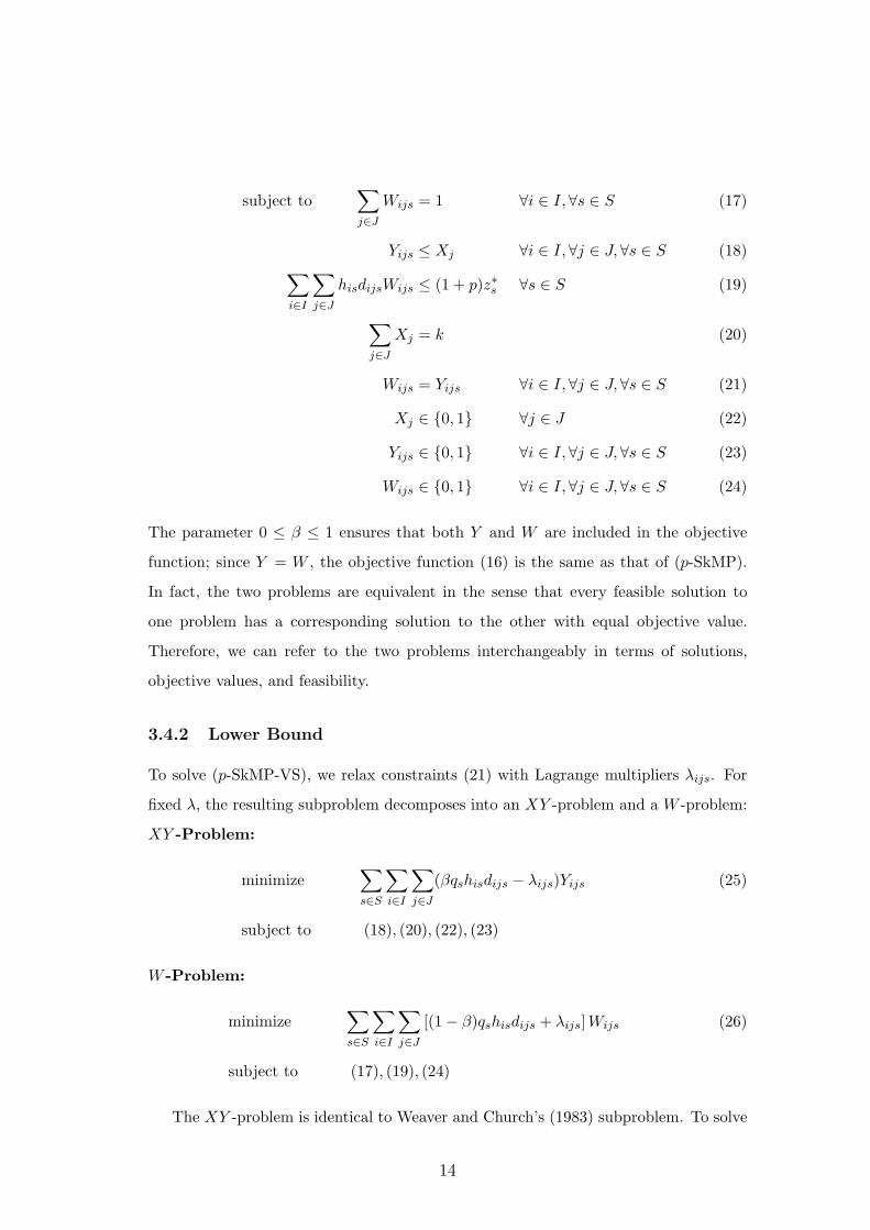
subject to∑
j∈J
Wijs = 1 ∀i ∈ I, ∀s ∈ S (17)
Yijs ≤ Xj ∀i ∈ I, ∀j ∈ J,∀s ∈ S (18)∑
i∈I
∑
j∈J
hisdijsWijs ≤ (1 + p)z∗s ∀s ∈ S (19)
∑
j∈J
Xj = k (20)
Wijs = Yijs ∀i ∈ I, ∀j ∈ J,∀s ∈ S (21)
Xj ∈ {0, 1} ∀j ∈ J (22)
Yijs ∈ {0, 1} ∀i ∈ I, ∀j ∈ J,∀s ∈ S (23)
Wijs ∈ {0, 1} ∀i ∈ I, ∀j ∈ J,∀s ∈ S (24)
The parameter 0 ≤ β ≤ 1 ensures that both Y and W are included in the objective
function; since Y = W , the objective function (16) is the same as that of (p-SkMP).
In fact, the two problems are equivalent in the sense that every feasible solution to
one problem has a corresponding solution to the other with equal objective value.
Therefore, we can refer to the two problems interchangeably in terms of solutions,
objective values, and feasibility.
3.4.2 Lower Bound
To solve (p-SkMP-VS), we relax constraints (21) with Lagrange multipliers λijs. For
fixed λ, the resulting subproblem decomposes into an XY -problem and a W -problem:
XY -Problem:
minimize∑
s∈S
∑
i∈I
∑
j∈J
(βqshisdijs − λijs)Yijs (25)
subject to (18), (20), (22), (23)
W -Problem:
minimize∑
s∈S
∑
i∈I
∑
j∈J
[(1− β)qshisdijs + λijs] Wijs (26)
subject to (17), (19), (24)
The XY -problem is identical to Weaver and Church’s (1983) subproblem. To solve
14

it, we compute the benefit bj of opening facility j:
bj =∑
s∈S
∑
i∈I
min{0, βqshisdijs − λijs}. (27)
We set Xj = 1 for the k facilities with smallest bj and set Yijs = 1 if Xj = 1 and
βqshisdijs − λijs < 0.
The W -problem reduces to |S| instances of the 0–1 multiple-choice knapsack prob-
lem (MCKP), an extension of the classical 0–1 knapsack problem in which the items
are partitioned into classes and exactly one item must be chosen from each class
(Nauss 1978, Sinha and Zoltners 1979). The MCKP does not naturally have all-integer
solutions, so the W -problem does not have the integrality property. The W -problem
can be formulated using the MCKP as follows. For each scenario s ∈ S, there is an
instance of the MCKP. Each instance contains |I| classes, each representing a retailer
i ∈ I. Each class contains |J | elements, each representing a facility j ∈ J . Item j in
class i has objective function coefficient (1 − β)qshisdijs + λijs and constraint coeffi-
cient hisdijs; including this item in the knapsack corresponds to assigning customer i
to facility j. The right-hand side of the knapsack constraint is (1 + p)z∗s .
The classical 0–1 knapsack problem can be reduced to the 0–1 MCKP, so the
MCKP is NP-hard. However, like the knapsack problem, effective algorithms have
been published for the MCKP, including algorithms based on linear programming
(Armstrong, Kung, Sinha and Zoltners 1983, Nakagawa, Kitao, Tsuji and Teraoka
2001, Pisinger 1995, Sinha and Zoltners 1979) and Lagrangian relaxation (Aggarwal,
Deo and Sarkar 1992). Any of these algorithms could be used to solve the W -problem,
with two caveats. The first is that the data must first be transformed into the form
required by a given algorithm (for example, transforming the sign of the coefficients,
the sense of the objective function, or the direction of the knapsack inequality), but
this can usually be done without difficulty. The second caveat is that either the MCKP
must be solved to optimality, or, if a heuristic is used, one must be chosen that can
return a lower bound on the optimal objective value; otherwise, the Lagrangian sub-
problem cannot be guaranteed to produce a lower bound for the problem at hand.
If the problem is solved heuristically, one might choose to set the variables using the
heuristic (upper-bound) solution, but then the lower bound used in the subgradient
optimization method does not match the actual value of the solution to the Lagrangian
15
subproblem. We have found this mismatch to lead to substantial convergence problems.
A better method is to use a lower-bound solution, not just the lower bound itself, to
set the variables. Not all heuristics that return lower bounds also return lower-bound
solutions, however, so care must be taken when making decisions about which MCKP
algorithm to use and how to set the variables.
Since the MCKP is NP-hard, we have elected to solve it heuristically by terminating
the branch-and-bound procedure of Armstrong et al. (1983) when it reaches a 1%
optimality gap. Their method can be modified to keep track not only of the best lower
bound at any point in the branch-and-bound tree, but also a solution attaining that
bound. These solutions, which are generally fractional, are then used as the values of
W in the Lagrangian subproblem.
3.4.3 Upper Bound
Once the XY - and W -problems have been solved, the two objective values are added
to obtain a lower bound on the objective function (3). An upper bound is obtained
at each iteration by opening the facilities for which Xj = 1 in the optimal solution to
(p-SkMP-VS) and assigning each customer i to the open facility that minimizes dijs.
This must be done for each scenario since the transportation costs may be scenario
dependent. The Lagrange multipliers are updated using subgradient optimization;
the method is standard, but the implementation is slightly different than in most
Lagrangian algorithms for facility location problems since the lower-bound solution
may be fractional. In addition, the subgradient optimization procedure requires an
upper bound to compute the step sizes, but it is possible that no feasible solution has
been found; we discuss an alternate upper bound in Section 5. The Lagrangian process
is terminated based on standard stopping criteria.
3.4.4 Initial Multipliers
As in any Lagrangian relaxation algorithm, the initial Lagrange multipliers can have
a significant impact on the final results. In our initial testing, we found that near-
optimal values of λijs tended to be large if j is an attractive facility for customer i in
scenario s, and small otherwise. Therefore, our strategy for setting initial mulitpliers
uses non-zero λijs values for the N closest facilities j to customer i in scenario s, with
16

larger values for closer facilities. In particular, the initial values for λ are given by
λijs =
γµN+2−kN+1 , if j is the kth closest facility to i in scenario s, for 1 ≤ k ≤ 10
0, otherwise(28)
where µ is the mean demand over all retailers and scenarios and γ is a user-specified
parameter. We use γ = 0.05 and N = 10 in our computational tests.
3.4.5 Branch and Bound
If the process terminates with an UB-LB gap that is larger than desired, or if no feasible
solution has been found, branch and bound is used to continue the search. Branching is
performed on the unfixed facility with the largest assigned demand in the best feasible
solution found at the current node. If no feasible solution has been found at the current
node but a feasible solution has been found elsewhere in the branch-and-bound tree,
that solution is used instead. If no feasible solution has been found anywhere in the
tree, an arbitrary facility is chosen for branching.
4 The p-SUFLP
In this section, we formulate the stochastic p-robust uncapacitated fixed charge location
problem (p-SUFLP) and then present a variable-splitting algorithm for it.
4.1 Formulation
In addition to the notation defined in Section 3.1, let fj be the fixed cost to open
facility j ∈ J . Since facility location decisions are scenario independent, so are the
fixed costs. (Strictly speaking, the fixed costs might be scenario dependent even if the
location decisions are made in the first stage. The expected fixed cost for facility j is
then given by(∑
s∈S qsfjs
)Xj = fjXj , in which case the objective function below is
still correct, with fj simply interpreted as the expected fixed cost. Constraints (32)
would also be modified to include fjs instead of fj . These changes would require only
trivial modifications to the algorithm proposed below.)
17
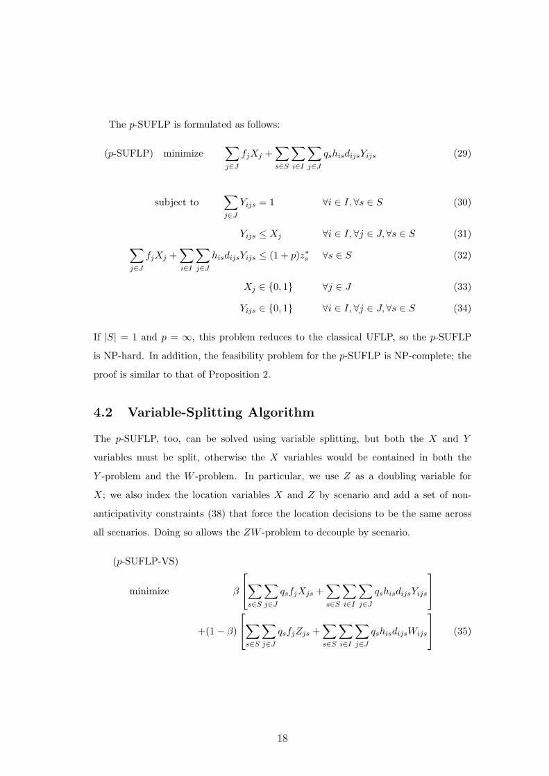
The p-SUFLP is formulated as follows:
(p-SUFLP) minimize∑
j∈J
fjXj +∑
s∈S
∑
i∈I
∑
j∈J
qshisdijsYijs (29)
subject to∑
j∈J
Yijs = 1 ∀i ∈ I, ∀s ∈ S (30)
Yijs ≤ Xj ∀i ∈ I, ∀j ∈ J,∀s ∈ S (31)∑
j∈J
fjXj +∑
i∈I
∑
j∈J
hisdijsYijs ≤ (1 + p)z∗s ∀s ∈ S (32)
Xj ∈ {0, 1} ∀j ∈ J (33)
Yijs ∈ {0, 1} ∀i ∈ I, ∀j ∈ J,∀s ∈ S (34)
If |S| = 1 and p = ∞, this problem reduces to the classical UFLP, so the p-SUFLP
is NP-hard. In addition, the feasibility problem for the p-SUFLP is NP-complete; the
proof is similar to that of Proposition 2.
4.2 Variable-Splitting Algorithm
The p-SUFLP, too, can be solved using variable splitting, but both the X and Y
variables must be split, otherwise the X variables would be contained in both the
Y -problem and the W -problem. In particular, we use Z as a doubling variable for
X; we also index the location variables X and Z by scenario and add a set of non-
anticipativity constraints (38) that force the location decisions to be the same across
all scenarios. Doing so allows the ZW -problem to decouple by scenario.
(p-SUFLP-VS)
minimize β
∑
s∈S
∑
j∈J
qsfjXjs +∑
s∈S
∑
i∈I
∑
j∈J
qshisdijsYijs
+(1− β)
∑
s∈S
∑
j∈J
qsfjZjs +∑
s∈S
∑
i∈I
∑
j∈J
qshisdijsWijs
(35)
18
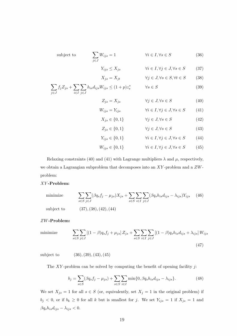
subject to∑
j∈J
Wijs = 1 ∀i ∈ I, ∀s ∈ S (36)
Yijs ≤ Xjs ∀i ∈ I, ∀j ∈ J,∀s ∈ S (37)
Xjs = Xjt ∀j ∈ J,∀s ∈ S,∀t ∈ S (38)∑
j∈J
fjZjs +∑
i∈I
∑
j∈J
hisdijsWijs ≤ (1 + p)z∗s ∀s ∈ S (39)
Zjs = Xjs ∀j ∈ J,∀s ∈ S (40)
Wijs = Yijs ∀i ∈ I, ∀j ∈ J,∀s ∈ S (41)
Xjs ∈ {0, 1} ∀j ∈ J,∀s ∈ S (42)
Zjs ∈ {0, 1} ∀j ∈ J,∀s ∈ S (43)
Yijs ∈ {0, 1} ∀i ∈ I, ∀j ∈ J,∀s ∈ S (44)
Wijs ∈ {0, 1} ∀i ∈ I, ∀j ∈ J,∀s ∈ S (45)
Relaxing constraints (40) and (41) with Lagrange multipliers λ and µ, respectively,
we obtain a Lagrangian subproblem that decomposes into an XY -problem and a ZW -
problem:
XY -Problem:
minimize∑
s∈S
∑
j∈J
(βqsfj − µjs)Xjs +∑
s∈S
∑
i∈I
∑
j∈J
(βqshisdijs − λijs)Yijs (46)
subject to (37), (38), (42), (44)
ZW -Problem:
minimize∑
s∈S
∑
j∈J
[(1− β)qsfj + µjs] Zjs +∑
s∈S
∑
i∈I
∑
j∈J
[(1− β)qshisdijs + λijs]Wijs
(47)
subject to (36), (39), (43), (45)
The XY -problem can be solved by computing the benefit of opening facility j:
bj =∑
s∈S
(βqsfj − µjs) +∑
s∈S
∑
i∈I
min{0, βqshisdijs − λijs}. (48)
We set Xjs = 1 for all s ∈ S (or, equivalently, set Xj = 1 in the original problem) if
bj < 0, or if bk ≥ 0 for all k but is smallest for j. We set Yijs = 1 if Xjs = 1 and
βqshisdijs − λijs < 0.
19
The ZW -problem reduces to |S| MCKP instances, one for each scenario. As in the
p-SkMP, there is a class for each customer i, each containing an item for each facility
j, representing the assignments Wijs; these items have objective function coefficient
(1−β)qshisdijs +λijs and constraint coefficient hisdijs. In addition, there is a class for
each facility j, representing the location decisions Zjs; these classes contain two items
each, one with objective function coefficient (1−β)qsfj +µjs and constraint coefficient
fj , representing opening the facility, and one with objective function and constraint
coefficient equal to 0, representing not opening the facility. The right-hand side of the
knapsack constraint equals (1 + p)z∗s .
We note that the p-SUFLP had even greater convergence problems than the p-
SkMP did when an upper-bound solution from the MCKP heuristic was used to set the
variables, rather than a lower-bound solution. This makes the selection of an MCKP
algorithm a critical issue for this problem. The approach outlined in Section 3.4 seems
to work quite well.
The upper-bounding, subgradient optimization, and branch-and-bound procedures
are as described above for the p-SkMP. The initial values of λ are set using (28), while
µis is initially set to 0 for all i and s.
5 Detecting Infeasibility
In this section, we focus our discussion on the p-SkMP for convenience, but all of the
results are easily duplicated for the p-SUFLP.
5.1 An A Priori Upper Bound
The subgradient optimization procedure used to update the Lagrange multipliers re-
quires an upper bound (call it UB). Typically, UB is the objective value of the best
known feasible solution, but Proposition 2 suggests that finding a feasible solution for
the p-SkMP (or p-SUFLP) is difficult, and there is no guarantee that one will be found
immediately or at all, even if one exists. We need a surrogate upper bound to use in
the step size calculation. Let
Q =∑
s∈S
qs(1 + p)z∗s . (49)
20
Proposition 3 If (p-SkMP) is feasible, then Q is an upper bound on its optimal ob-
jective value.
Proof. Let (X∗, Y ∗) be an optimal solution for (p-SkMP) . The objective value under
solution (X∗, Y ∗) is
∑
s∈S
qszs(X∗, Y ∗) ≤∑
s∈S
qs(1 + p)z∗s = Q (50)
by constraints (6).
We refer to Q as the a priori upper bound. Proposition 3 has two important uses.
First, if no feasible solution has been found as of a given iteration, we set UB = Q in
the step-size calculation. Second, we can use Proposition 3 to detect when the problem
is infeasible. In particular, if the Lagrangian procedure and/or the branch-and-bound
procedure yield a lower bound greater than Q, we can terminate the procedure and
conclude that the problem is infeasible. One would like the Lagrangian procedure to
yield bounds greater than Q whenever the problem is infeasible, providing a test for
feasibility in every case. Unfortunately, there are infeasible instances for which the
Lagrangian bound is less than Q. In the next section, we investigate the circumstances
under which we can expect to find Lagrange multipliers that yield a bound greater
than Q.
5.2 Lagrangian Unboundedness
Let (p-SLR) be the Lagrangian subproblem obtained by relaxing (21) in (p-SkMP-VS);
(p-SLR) consists of both the XY -problem and the W -problem. Let Lλ,µ be the objec-
tive value of (p-SLR) under given multipliers λ, µ (i.e., the sum of the optimal objective
values of the XY - and W -problems). Let (p-SPMP-VS) be the LP relaxation of (p-
SkMP-VS). It is possible that (p-SkMP-VS) is infeasible but (p-SPMP-VS) is feasible.
When this is the case, we know that the optimal objective value of (p-SLR) is at least as
great as that of (p-SPMP-VS) (from standard Lagrangian duality theory), but we can-
not say whether it is greater than Q. On the other hand, if (p-SPMP-VS) is infeasible,
corollary 1 below demonstrates that (p-SLR) is either infeasible or unbounded—i.e.,
if (p-SLR) is feasible, then for any M ∈ R, there exist multipliers λ, µ such that
Lλ,µ > M . We first state this result for general linear programs:
21
Lemma 1 Let (P) be a linear program of the form
(P) minimize cx
subject to Ax = b
Dx ≤ e
x ≥ 0
with c ≥ 0, and let (LR) be the Lagrangian relaxation obtained by relaxing the con-
straints Ax = b. If (P) is infeasible, then (LR) is either infeasible or unbounded. That
is, either (LR) is infeasible or for any M ∈ R, there exist Lagrange multipliers λ such
that the objective value of (LR) under λ is greater than M .
It is well known that for feasible problems, the Lagrangian dual (LR) and the LP dual
behave similarly; the lemma verifies that the same intuition holds even for infeasible
problems. The proof is similar to standard proofs that the Lagrangian bound is at
least as great as the LP bound for integer programming problems (Nemhauser and
Wolsey 1988) and is omitted here.
Corollary 1 If (p-SPMP-VS) is infeasible, then (p-SLR) is either infeasible or un-
bounded.
Proof. By Lemma 1, the LP relaxation of (p-SLR) is either infeasible or unbounded.
(The equality in (17) can be replaced by ≥ and that in (20) can be replaced by ≤WLOG; (17) can then be multiplied by −1 to obtain an LP in the form used in
Lemma 1. The non-negativity of the objective function coefficients follows from the
definitions of the parameters.) If the LP relaxation of (p-SLR) is infeasible, then (p-
SLR) must be as well, and similarly, if the LP relaxation of (p-SLR) is unbounded, then
(p-SLR) must be as well. Therefore (p-SLR) itself is either infeasible or unbounded.
In most cases, if (p-SPMP-VS) is infeasible, then (p-SLR) will be unbounded (not
infeasible). (p-SLR) is infeasible if one of the constituent MCKPs is infeasible; since
the constraints are independent of λ and µ, the problem is infeasible for any set of
Lagrange multipliers and should be identified as such by the MCKP algorithm. If
(p-SLR) is infeasible, then clearly (p-SkMP-VS) is infeasible since the constraints of
the former problem are a subset of those of the latter. This rarely occurs, however,
22
since most customers have a close (or even co-located) facility to which they may be
assigned in the W -problem. Therefore, in most cases, if (p-SPMP-VS) is infeasible,
the Lagrangian is unbounded, in which case the subgradient optimization procedure
should find λ and µ such that Lλ,µ > Q and the algorithm can terminate with a
proof of infeasibility. If (p-SPMP-VS) is feasible but (p-SkMP-VS) is not, this method
cannot detect infeasibility, and an extensive search of the branch-and-bound tree may
be required before infeasibility can be proven.
6 The Minimax Regret Heuristic
For a given optimization problem with uncertain parameters, the minimax regret prob-
lem is to find a solution that minimizes the maximum regret across all scenarios. Min-
imax regret is a commonly used robustness measure, especially for problems in which
scenario probabilities are unknown. One can solve the minimax regret kMP heuristi-
cally using the algorithm discussed above by systematically varying p and solving (p-
SkMP) for each value, as outlined below. (We focus our discussion on the (p-SkMP),
but the method for the (p-SUFLP) is identical.) If scenario probabilities are unknown,
qs can be set to 1/|S| for all s. (p-SkMP) does not need to be solved to optimality:
the algorithm can terminate as soon as a feasible solution is found for the current p.
The smallest value of p for which the problem is feasible corresponds to the minimax
regret value.
We introduce this method as a heuristic, rather than as an exact algorithm, because
for some values of p, (p-SkMP) may be infeasible while its LP relaxation is feasible. As
discussed in Section 5.2, infeasibility may not be detected by the Lagrangian method
in this case, and may not be detected until a sizable portion of the branch-and-bound
tree has been explored. Nevertheless, depending on the patience of the modeler, the
method’s level of accuracy can be adjusted as desired; this point is explicated in the
discussion of step 2, below.
Our heuristic for solving the minimax regret kMP returns two values, pL and pU ;
the minimax regret is guaranteed to be in the range (pL, pU ]. The heuristic also returns
a solution whose maximum regret is pU . It works by maintaining four values, pL ≤pL ≤ pU ≤ pU (see Figure 2). At any point during the execution of the heuristic, the
23

problem is known to be infeasible for p ≤ pL and feasible for p ≥ pU ; for p ∈ [pL, pU ], the
problem is indeterminate (i.e., feasibility has been tested but could not be determined);
and for p ∈ (pL, pL) or (pU , pU ), feasibility has not been tested. At each iteration, a
value of p is chosen in (pL, pL) or (pU , pU ) (whichever range is larger), progressively
reducing these ranges until they are both smaller than some pre-specified tolerance ε.
[Insert Figure 2 here.]
Algorithm 1 (MINIMAX-REGRET)
0. Determine a lower bound pL for which (p-SkMP) is known to be infeasible and
an upper bound pU for which (p-SkMP) is known to be feasible. Let (X∗, Y ∗) be
a feasible solution with maximum regret pU . Mark pL and pU as undefined.
1. If pL and pU are undefined, let p ← (pL + pU )/2; else if pL − pL > pU − pU , let
p ← (pL + pL)/2; else, let p ← (pU + pU )/2.
2. Determine the feasibility of (p-SkMP) under the current value of p.
2.1 If (p-SkMP) is feasible, let pU ← the maximum relative regret of the solution
found, let (X∗, Y ∗) be the solution found in step 2, and go to step 3.
2.2 Else if (p-SkMP) is infeasible, let pL ← p and go to step 3.
2.3 Else [(p-SkMP) is indeterminate]: If pL and pU are undefined, let pL ← p
and pU ← p and mark pL and pU as defined; else if p ∈ (pL, pL), let pL ← p;
else [p ∈ (pU , pU )], let pU ← p. Go to step 3.
3. If pL − pL < ε and pU − pU < ε, stop and return pL, pU , (X∗, Y ∗). Else, go to
step 2.
Several comments are in order. In step 0, the lower bound pL can be determined
by choosing a small enough value that the problem is known to be infeasible (e.g., 0).
The upper bound can be determined by solving (p-SkMP) with p = ∞ and setting
pU equal to the maximum regret value from the solution found; this solution can also
be used as (X∗, Y ∗). In step 1, we are performing a binary search on each region.
More efficient line searches, such as the Golden Section search, would work as well, but
we use the binary search for ease of exposition. In step 2, the instruction “determine
the feasibility...” is to be carried out by solving (p-SkMP) until (a) a feasible solution
has been found [the problem is feasible], (b) the lower bound exceeds the a priori
24
upper bound Q [the problem is infeasible], or (c) a pre-specified stopping criterion has
been reached [the problem is indeterminate]. This stopping criterion may be specified
as a number of Lagrangian iterations, a number of branch-and-bound nodes, a time
limit, or any other stopping criterion desired by the user. In general, if the stopping
criterion is more generous (i.e., allows the algorithm to run longer), fewer problems
will be indeterminate, and the range (pL, pU ] returned by the heuristic will be smaller.
One can achieve any desired accuracy by adjusting the stopping criterion, though if a
small range is desired, long run times might ensue. (Finding an appropriate stopping
criterion may require some trial and error; it is not an immediate function of the desired
accuracy.) Our heuristic therefore offers two important advantages over most heuristics
for minimax regret problems: (1) it provides both a candidate minimax-regret solution
and a lower bound on the optimal minimax regret, and (2) it can be modified to achieve
any desired level of accuracy.
7 Computational Results
7.1 Algorithm Performance
7.1.1 Experimental Design
We tested the variable-splitting algorithms for the p-SkMP and p-SUFLP on four
benchmark data sets from the facility location literature and ten randomly gener-
ated data sets. The benchmark data sets consist of the 55-node problem of Swain
(1971) (see Church and Weaver (1986) for the complete data set) and the 49-, 88-, and
150-node data sets of Daskin (1995), which are derived from 1990 U.S. census data.
Because the benchmark data sets each include only a single scenario, we generated
additional scenarios randomly, as described below. In all data sets, each node serves as
both a customer and a potential facility site (i.e., I = J). The data sets were derived
as follows1:
• Census Data. The 49-, 88-, and 150-node data sets consist of U.S. cities. We
computed the “base” demand by dividing the population given by Daskin (1995)
1All data sets may be obtained from the lead author’s web site, www.lehigh.edu/∼lvs2/research.html.
25
by 1000; we then used these base demands to compute scenario-specific demands
for 9 scenarios following the method described by Daskin, Hesse and ReVelle
(1997); in brief, this method involves defining an “attractor” point for each sce-
nario and scaling each retailer’s demand based on its distance to the attractor
point. The total mean demand is the same in all scenarios for a given problem.
Fixed location costs (fj) for the p-SUFLP were obtained by dividing the fixed
cost given by Daskin (1995) by 10 for the 49-node data set and by 100 for the
88-node data set; for the 150-node data set, fixed costs for all retailers were set to
1000. Retailer locations were taken directly from Daskin (1995) for all three data
sets; for scenarios 2–9, the latitute and longitude values from scenario 1 were mul-
tiplied by random numbers drawn uniformly from U [0.95, 1.05] (i.e., perturbed
randomly by up to 5% in either direction). This has the effect of making distances
scenario specific. Per-unit transportation costs were set equal to the great-circle
distances between facilities and customers. The scenario probabilities are taken
from Daskin et al. (1997) and are given by 0.01, 0.04, 0.15, 0.02, 0.34, 0.14, 0.09,
0.16, 0.05. We will refer to these data sets as Census49-9, Census88-9, and
Census150-9, respectively.
• Random Data. We generated 10 data sets randomly, each with 50 nodes and 5
scenarios. In each data set, demands for scenario 1 were drawn uniformly from
[0, 10000] and rounded to the nearest integer, and x and y coordinates were drawn
uniformly from [0, 1]. In scenarios 2 through 5, demands were obtained by multi-
plying scenario-1 demands by a random number drawn uniformly from [0.5, 1.5]
and rounding off; similarly, x and y coordinates were obtained by multiplying
scenario-1 coordinates by a random number drawn uniformly from [0.75, 1.25].
Per-unit transportation costs were set equal to the Euclidean distances between
facilities and customers. Fixed costs for the p-SUFLP were drawn uniformly from
[4000, 8000] and rounded to the nearest integer. Scenario probabilities were set
as follows: q1 was drawn uniformly from (0, 1), qt was drawn uniformly from(0, 1−∑t−1
s=1 qs
)for t = 2, 3, 4, and q5 was set to 1 −∑4
s=1 qs. We will refer to
these data sets as Random50-5.
• Swain Data. The Swain data set contains 55 nodes, for which we generated 5
scenarios. Scenario 1 demands and coordinates were set to Swain’s original data.
26
Demands for scenarios 2–5 were obtained by multiplying scenario-1 demands by
a [0.5, 1.5] random variate and rounding off; x and y coordinates in those scenar-
ios were obtained by multiplying scenario-1 coordinates by a U [0.5, 1.5] random
variate and rounding off. Per-unit transportation costs were set equal to the Eu-
clidean distances between facilities and customers. Fixed costs for the p-SUFLP
were set to 1000 for all facilities. Scenario probabilities were set to 0.2 for each
scenario. We will refer to this data set as Swain55-5.
The performance measure of interest for these tests is the tightness of the bounds
produced at the root node; consequently, no branching was performed. We termi-
nated the Lagrangian procedure when the LB–UB gap was less than 1%, when 1200
Lagrangian iterations had elapsed, or when α (a parameter used in the subgradient
optimization procedure; see Daskin (1995)) was less than 10−8. Initial Lagrange mul-
tipliers were set for the p-SkMP and p-SUFLP as described in Sections 3.4.4 and 4.2,
respectively. The weighting coefficient β was set to 0.2. We tested our algorithms for
several values of p. The algorithm was coded in C++ and executed on a Gateway
M210 notebook computer with a 1.5 GHz Intel Pentium M processor and 992 MB of
RAM running under Windows XP Professional.
7.1.2 Optimality Gaps and Feasibility
Table 1 summarizes the algorithms’ performance for both the p-SkMP and the p-
SUFLP. The column marked “k” gives the number of facilities to locate for the p-SkMP
or “—” for the p-SUFLP. The column marked “p” gives the robustness coefficient.
The “Gap” columns give the mean and maximum values of (UB− LB)/LB among all
problems (out of 14) for which a feasible solution was found. Note that for some values
of p, no feasible solution was found for any of the 14 test problems. “# Lag Iter”
gives the mean and maximum number of Lagrangian iterations performed across all
problems. The final column lists the number of problems (out of 14) for which feasibility
was proved (i.e., a feasible solution was found), the number for which infeasibility was
proved (i.e., the lower bound exceeded Q), and the number that were indeterminate
(i.e., no feasible solution was found but the problem could not be proven infeasible).
[Insert Table 1 here.]
27
The algorithms generally attained gaps of no more than a few percent for feasible
instances. Tighter bounds may be desirable, especially if the modeler intends to find
a provably optimal solution using branch and bound. These instances generally re-
quired close to the maximum allowable number of Lagrangian iterations. On the other
hand, the provably infeasible instances generally required fewer than 100 iterations
to prove infeasibility. The algorithm was generally successful in proving feasibility or
infeasibility, with 52 out of 392 total instances (13%) left indeterminate, generally with
mid-range values of p. Corollary 1 implies that for these problems, either the LP re-
laxation is feasible or it is infeasible but we are not finding good enough multipliers to
exceed Q. Further research is needed to establish which is the case.
7.1.3 CPU Times
Table 2 indicates the time spent solving the test problems, broken down by data set.
For the Random50-5 data sets, both mean and maximum times (over 10 trials) are
reported. The algorithm generally required well under one minute to execute on a
notebook computer. (The exception is Census150-9, which required nearly four minutes
on average. However, this is not surprising since this is a large problem, roughly
equivalent to a deterministic problem with 1350 nodes.) The bulk of the execution
time (80% on average) was spent solving multiple-choice knapsack problems, and this
statistic is relatively constant across problems of various sizes.
[Insert Table 2 here.]
7.2 Minimax Regret Heuristic
We tested the minimax regret heuristic discussed in Section 6 for the p-SkMP and p-
SUFLP using the 14 data sets described above. As above, no branching was performed,
and an iteration limit of 1200 was used (this represents the stopping criteria in step 2 of
the heuristic). The results are summarized in Table 3. The first column indicates the
data set, while the second indicates the value of k (or “—” for the p-SUFLP instances).
The columns marked “pL” and “pU” indicate the lower and upper bounds on the
minimax regret value returned by the heuristic. The column marked “Gap” gives the
difference between pU and pL, while the “Init Gap” column gives the gap between the
28

values of pU and pL used to initialize the heuristic in step 0. (Since pL was initially set
to 0, the “Init Gap” column equals the maximum regret of the unconstrained problem,
used to initialize pU .) The column marked “CPU Time” indicates the time (in seconds)
spent by the heuristic, while that marked “# Solved” indicates the number of problems
solved by the heuristic (i.e., the number of values of p required before termination).
For the Random50-5 problems, all values are means taken over the 10 instances.
[Insert Table 3 here.]
The heuristic generally returned ranges of about 7% for the p-SkMP and 4% that
for the p-SUFLP. As discussed above, these ranges could be reduced by using a more
lenient stopping criterion—for example, using branch-and-bound after processing at
the root node. It is our suspicion that pU is closer to the true minimax regret value
than pL is (that is, the upper bound returned by the heuristic is tighter than the lower
bound), though further research is needed to establish this definitively.
7.3 Cost vs. Regret
The main purpose of the p-SkMP and p-SUFLP is to reduce the maximum regret (by
the choice of p) with as little increase in expected cost as possible. To illustrate this
tradeoff, we used the constraint method of multi-objective programming (Cohon 1978)
to generate a tradeoff curve between the expected cost and the maximum regret. In
particular, we solved the problem with p = ∞ and recorded the objective value and
maximum regret of the solution; we then set p equal to the actual maximum regret
obtained minus 0.00001 and re-solved the problem, continuing this process until no
feasible solution could be found for a given value of p.
We performed this experiment for two representative data sets: Census49-9 for the
p-SkMP (with k = 25) and one of the Random50-5 data sets for the p-SUFLP. The
results are summarized in Table 4. The column marked “p” gives the value of p used
to solve the problem; “Obj Value” is the objective value of the best feasible solution
returned by the algorithm; “% Increase” is the percentage by which the objective value
is greater than that of the solution found using p = ∞; “Max Regret” is the maximum
relative regret of the best solution found; and “% Decrease” is the percentage by which
the maximum regret is smaller than that of the solution found using p = ∞. The
29

expected cost and maximum regret are plotted in Figure 3 for both problems (the
regret values for the Random50-5 data set appear on the right-hand y-axis).
[Insert Table 4 here.]
[Insert Figure 3 here.]
It is clear that large reductions in maximum regret are possible with small increases
in expected cost. For example, the sixth solution for the p-SkMP represents a 33%
reduction in maximum regret with only a 1% increase in expected cost, and the last p-
SUFLP solution attains a 78% reduction in maximum regret with only a 0.7% increase
in expected cost. These results justify the stochastic p-robust approach since it costs
very little to “buy” robustness. This is evident from Figure 3 since the tradeoff curves
are steep—large reductions in regret are possible with small increases in expected
cost. While we cannot be assured that results like these would be attained for any
instance, we have found them to be representative of the general trend. Note that not
all problems were solved to optimality (because no branching was performed), so it
is possible that for some problems, the optimal expected costs are even smaller than
those listed in the table.
8 Conclusions
In this paper we presented models that seek the minimum-expected-cost solution for
two classical facility location problems, subject to the constraint that the solution cho-
sen must have relative regret no more than p in every scenario. This robustness mea-
sure, called stochastic p-robustness, combines the advantages of traditional stochastic
and robust optimization approaches. We presented algorithms for our models that use
variable splitting, or Lagrangian decomposition. The Lagrangian subproblems split
into two problems, one problem that can be solved by inspection and another that re-
duces to the multiple-choice knapsack problem. We showed that our algorithm can be
used iteratively to solve the minimax-regret problem; this method is approximate, but
it provides both lower and upper bounds on the minimax regret value, and it can be
adjusted to provide arbitrarily close bounds. In addition, we showed empirically that
large reductions in regret are possible with small increases in expected cost. Although
our discussion is focused on relative regret, our models and algorithms can be readily
30
applied to problems involving absolute regret or simply the cost in each scenario.
While the bounds provided by our algorithms are reasonable, it would be desirable
to tighten them even further. Preliminary exploration of our formulations indicates
that the objective values of the IPs grow much more quickly as p decreases than the
objective values of their LP relaxations do. This means that for more tightly con-
strained problems, the LP bounds are increasingly weak. While the Lagrangian bound
is necessarily greater than the LP bound (because the subproblems do not have the
integrality property), it may not be great enough to provide sufficiently tight bounds.
We have begun investigating the reasons for this discrepancy in the bounds and possible
methods for improvement; we expect this to be an avenue for future research.
Finally, we note that Snyder (2003) applies the stochastic p-robustness measure to
the location model with risk-pooling (LMRP; Daskin, Coullard and Shen (2002), Shen,
Coullard and Daskin (2003), a recent supply chain design model that is based on the
UFLP but incorporates risk-pooling effects and economies of scale in inventory costs.
The stochastic p-robust LMRP formulation does not lend itself to a variable-splitting
approach because of the non-linearity of the objective function; instead, Snyder (2003)
solves the problem using standard Lagrangian relaxation. We consider the application
of stochastic p-robustness to other logistics and supply chain design problems to be
another avenue for future research.
9 Acknowledgments
This research was supportd by NSF Grants DMI-9634750 and DMI-9812915. This
support is gratefully acknowledged. The authors also wish to thank two anonymous
referees for several helpful suggestions.
References
Aggarwal, V., Deo, N. and Sarkar, D. (1992), The knapsack problem with disjoint
multiple-choice constraints, Naval Research Logistics 39(2), 213–227.
31

Armstrong, R. D., Kung, D. S., Sinha, P. and Zoltners, A. A. (1983), A computational
study of a multiple-choice knapsack algorithm, ACM Transactions on Mathemat-
ical Software 9(2), 184–198.
Averbakh, I. and Berman, O. (2000), Minmax regret median location on a network
under uncertainty, INFORMS Journal on Computing 12(2), 104–110.
Balinski, M. L. (1965), Integer programming: Methods, uses, computation, Manage-
ment Science 12(3), 253–313.
Barcelo, J., Fernandez, E. and Jornsten, K. O. (1991), Computational results from a
new Lagrangean relaxation algorithm for the capacitated plant location problem,
European Journal of Operational Research 53(1), 38–45.
Brandeau, M. L. and Chiu, S. S. (1989), An overview of representative problems in
location research, Management Science 35(6), 645–674.
Burkard, R. E. and Dollani, H. (2001), Robust location problems with pos/neg weights
on a tree, Networks 38(2), 102–113.
Chen, B. and Lin, C.-S. (1998), Minmax-regret robust 1-median location on a tree,
Networks 31(2), 93–103.
Church, R. L. and Weaver, J. R. (1986), Theoretical links between median and coverage
location problems, Annals of Operations Research 6, 1–19. contains complete
Swain (1971) data set.
Cohon, J. L. (1978), Multiobjective programming and planning, Mathematics in Science
and Engineering, Academic Press, New York.
Cornuejols, G., Fisher, M. L. and Nemhauser, G. L. (1977), Location of bank accounts
to optimize float: An analytic study of exact and approximate algorithms, Man-
agement Science 23(8), 789–810.
Cornuejols, G., Sridharan, R. and Thizy, J. (1991), A comparison of heuristics and
relaxations for the capacitated plant location problem, European Journal of Op-
erational Research 50, 280–297.
Current, J., Daskin, M. S. and Schilling, D. (2002), Discrete network location models,
in Z. Drezner and H. W. Hamacher, eds, ‘Facility Location: Applications and
Theory’, Springer-Verlag, New York, chapter 3.
32

Current, J., Ratick, S. and ReVelle, C. (1997), Dynamic facility location when the total
number of facilities is uncertain: A decision analysis approach, European Journal
of Operational Research 110(3), 597–609.
Daskin, M. S. (1995), Network and Discrete Location: Models, Algorithms, and Appli-
cations, Wiley, New York.
Daskin, M. S. (2004), SITATION software. Available for download from
users.iems.northwestern.edu/∼msdaskin/.
Daskin, M. S., Coullard, C. R. and Shen, Z.-J. M. (2002), An inventory-location model:
Formulation, solution algorithm and computational results, Annals of Operations
Research 110, 83–106.
Daskin, M. S., Hesse, S. M. and ReVelle, C. S. (1997), α-reliable p-minimax regret: A
new model for strategic facility location modeling, Location Science 5(4), 227–246.
Garey, M. R. and Johnson, D. S. (1979), Computers and Intractability: A Guide to the
Theory of NP-Completeness, W. H. Freeman and Company, New York.
Geoffrion, A. (1974), Lagrangean relaxation for integer programming, Mathematical
Programming Study 2, 82–114.
Guignard, M. and Kim, S. (1987), Lagrangean decomposition: A model yielding strong
Lagrangean bounds, Mathematical Programming 39, 215–228.
Gutierrez, G. J. and Kouvelis, P. (1995), A robustness approach to international sourc-
ing, Annals of Operations Research 59, 165–193.
Gutierrez, G. J., Kouvelis, P. and Kurawarwala, A. A. (1996), A robustness approach
to uncapacitated network design problems, European Journal of Operational Re-
search 94, 362–376.
Hakimi, S. L. (1964), Optimum locations of switching centers and the absolute centers
and medians of a graph, Operations Research 12(3), 450–459.
Hakimi, S. L. (1965), Optimum distribution of switching centers in a communica-
tion network and some related graph theoretic problems, Operations Research
13(3), 462–475.
33
Kouvelis, P., Kurawarwala, A. A. and Gutierrez, G. J. (1992), Algorithms for robust
single and multiple period layout planning for manufacturing systems, European
Journal of Operational Research 63, 287–303.
Kouvelis, P. and Yu, G. (1997), Robust Discrete Optimization and its Applications,
Kluwer Academic Publishers, Boston.
Louveaux, F. V. (1993), Stochastic location analysis, Location Science 1(2), 127–154.
Mirchandani, P. B., Oudjit, A. and Wong, R. T. (1985), ‘Multidimensional’ exten-
sions and a nested dual approach for the m-median problem, European Journal
of Operational Research 21(1), 121–137.
Nakagawa, Y., Kitao, M., Tsuji, M. and Teraoka, Y. (2001), Calculating the upper
bound of the multiple-choice knapsack problem, Electronics and Communications
in Japan Part 3 84(7), 22–27.
Nauss, R. (1978), The 0-1 knapsack problem with multiple choice constraints, European
Journal of Operational Research 2, 125–131.
Nemhauser, G. L. and Wolsey, L. A. (1988), Integer and Combinatorial Optimization,
Wiley, New York.
Owen, S. H. and Daskin, M. S. (1998), Strategic facility location: A review, European
Journal of Operational Research 111(3), 423–447.
Pisinger, D. (1995), A minimal algorithm for the multiple-choice knapsack problem,
European Journal of Operational Research 83(2), 394–410.
Serra, D. and Marianov, V. (1998), The p-median problem in a changing network: The
case of Barcelona, Location Science 6, 383–394.
Serra, D., Ratick, S. and ReVelle, C. (1996), The maximum capture problem with
uncertainty, Environment and Planning B 23, 49–59.
Shen, Z.-J. M., Coullard, C. R. and Daskin, M. S. (2003), A joint location-inventory
model, Transportation Science 37(1), 40–55.
Sheppard, E. S. (1974), A conceptual framework for dynamic location-allocation anal-
ysis, Environment and Planning A 6, 547–564.
Sinha, P. and Zoltners, A. A. (1979), The multiple-choice knapsack problem, Operations
Research 27(3), 503–515.
34
Snyder, L. V. (2003), Supply Chain Robustness and Reliability: Models and Algo-
rithms, PhD thesis, Northwestern University.
Snyder, L. V. (2005a), Facility location under uncertainty: A review, forthcoming in
IIE Transactions .
Snyder, L. V. (2005b), A note on the robust international sourcing algorithm of
Gutierrez and Kouvelis, submitted for publication.
Swain, R. (1971), A Decomposition Algorithm for a Class of Facility Location Problems,
PhD thesis, Cornell University, Ithaca, NY.
Vairaktarakis, G. L. and Kouvelis, P. (1999), Incorporation dynamic aspects and un-
certainty in 1-median location problems, Naval Research Logistics 46(2), 147–168.
Weaver, J. R. and Church, R. L. (1983), Computational procedures for location prob-
lems on stochastic networks, Transportation Science 17(2), 168–180.
35

Figure and Table Captions
Figure 1: p-SkMP instance.
Figure 2: Ranges maintained by the minimax-regret heuristic.
Figure 3: Expected cost vs. maximum regret.
Table 1: Algorithm performance: Optimality gaps and feasibility.
Table 2: Algorithm performance: CPU times.
Table 3: Minimax regret heuristic performance.
Table 4: Expected cost vs. maximum regret.
36
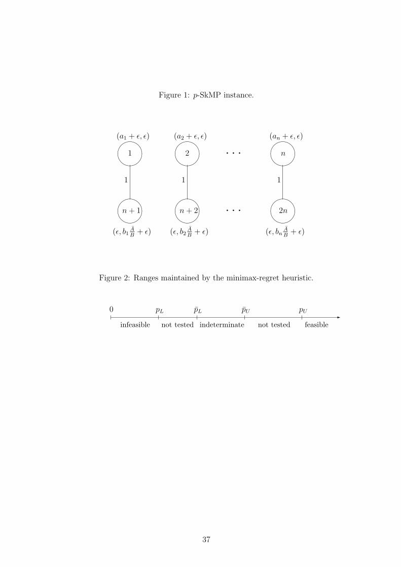
Figure 1: p-SkMP instance.
"!
#Ã
"!
#Ã
"!
#Ã
"!
#Ã
"!
#Ã
"!
#Ã1 2 n
n + 1 n + 2 2n
1 1 1
(a1 + ε, ε) (a2 + ε, ε) (an + ε, ε)
(ε, b1AB
+ ε) (ε, b2AB
+ ε) (ε, bnAB
+ ε)
. . .
. . .
Figure 2: Ranges maintained by the minimax-regret heuristic.
-0 pL pL pU pU
infeasible not tested indeterminate not tested feasible
37
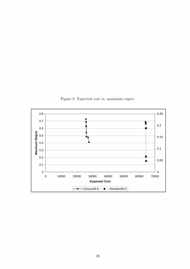
Figure 3: Expected cost vs. maximum regret.
0
0.1
0.2
0.3
0.4
0.5
0.6
0.7
0.8
0 10000 20000 30000 40000 50000 60000 70000
Expected Cost
Max
imu
m R
egre
t
0
0.05
0.1
0.15
0.2
0.25
Census49-9 Random50-5
38
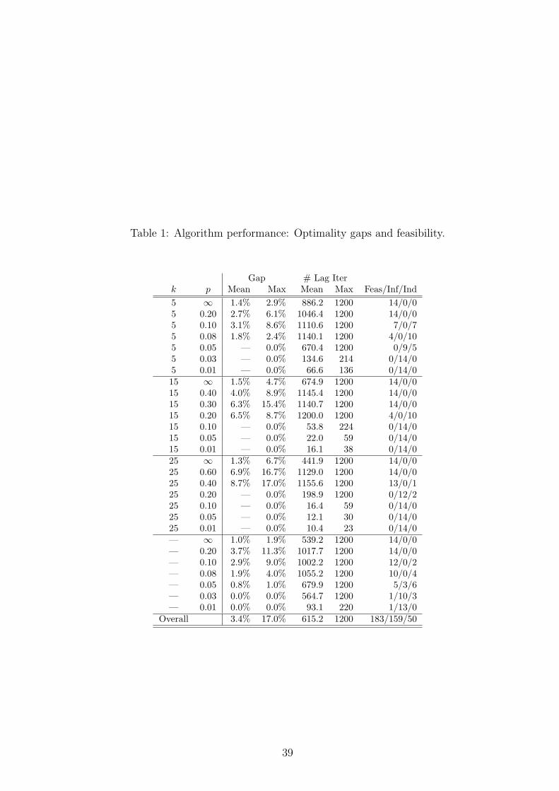
Table 1: Algorithm performance: Optimality gaps and feasibility.
Gap # Lag Iterk p Mean Max Mean Max Feas/Inf/Ind5 ∞ 1.4% 2.9% 886.2 1200 14/0/05 0.20 2.7% 6.1% 1046.4 1200 14/0/05 0.10 3.1% 8.6% 1110.6 1200 7/0/75 0.08 1.8% 2.4% 1140.1 1200 4/0/105 0.05 — 0.0% 670.4 1200 0/9/55 0.03 — 0.0% 134.6 214 0/14/05 0.01 — 0.0% 66.6 136 0/14/015 ∞ 1.5% 4.7% 674.9 1200 14/0/015 0.40 4.0% 8.9% 1145.4 1200 14/0/015 0.30 6.3% 15.4% 1140.7 1200 14/0/015 0.20 6.5% 8.7% 1200.0 1200 4/0/1015 0.10 — 0.0% 53.8 224 0/14/015 0.05 — 0.0% 22.0 59 0/14/015 0.01 — 0.0% 16.1 38 0/14/025 ∞ 1.3% 6.7% 441.9 1200 14/0/025 0.60 6.9% 16.7% 1129.0 1200 14/0/025 0.40 8.7% 17.0% 1155.6 1200 13/0/125 0.20 — 0.0% 198.9 1200 0/12/225 0.10 — 0.0% 16.4 59 0/14/025 0.05 — 0.0% 12.1 30 0/14/025 0.01 — 0.0% 10.4 23 0/14/0— ∞ 1.0% 1.9% 539.2 1200 14/0/0— 0.20 3.7% 11.3% 1017.7 1200 14/0/0— 0.10 2.9% 9.0% 1002.2 1200 12/0/2— 0.08 1.9% 4.0% 1055.2 1200 10/0/4— 0.05 0.8% 1.0% 679.9 1200 5/3/6— 0.03 0.0% 0.0% 564.7 1200 1/10/3— 0.01 0.0% 0.0% 93.1 220 1/13/0
Overall 3.4% 17.0% 615.2 1200 183/159/50
39
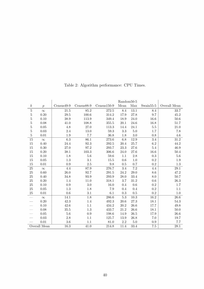
Table 2: Algorithm performance: CPU Times.
Random50-5k p Census49-9 Census88-9 Census150-9 Mean Max Swain55-5 Overall Mean5 ∞ 21.5 85.2 272.5 8.4 13.1 8.4 33.75 0.20 29.5 100.6 314.2 17.9 27.8 9.7 45.25 0.10 38.9 113.9 349.4 18.9 24.0 16.6 50.65 0.08 41.0 108.8 355.5 20.1 24.6 16.8 51.75 0.05 4.8 27.0 113.3 14.4 24.1 5.5 21.05 0.03 2.4 13.0 59.3 3.3 5.0 1.7 7.85 0.01 1.9 7.7 36.8 1.8 3.0 0.8 4.615 ∞ 6.3 86.1 273.6 6.8 12.9 3.4 31.215 0.40 24.4 92.3 292.5 20.4 25.7 6.2 44.215 0.30 27.0 97.2 293.7 23.3 27.6 5.4 46.915 0.20 38.1 103.3 306.6 24.0 27.6 16.6 50.415 0.10 1.8 5.6 59.6 1.1 2.8 0.3 5.615 0.05 1.3 3.1 15.5 0.6 1.0 0.2 1.915 0.01 0.9 2.5 9.8 0.5 0.7 0.2 1.325 ∞ 4.4 87.9 276.7 3.4 7.2 4.4 29.125 0.60 26.0 92.7 291.5 24.2 29.0 8.6 47.225 0.40 34.8 93.9 293.9 28.0 33.4 8.0 50.725 0.20 1.4 11.0 318.1 3.7 31.2 0.6 26.325 0.10 0.9 3.0 16.0 0.4 0.6 0.2 1.725 0.05 1.3 1.8 7.9 0.4 0.4 0.2 1.125 0.01 0.6 3.1 6.1 0.3 0.5 0.2 1.0— ∞ 14.1 1.8 286.6 5.3 10.3 16.2 26.6— 0.20 42.3 1.4 492.3 20.6 27.3 18.1 54.3— 0.10 42.6 1.1 434.2 20.2 26.6 17.7 49.8— 0.08 35.5 1.3 433.7 21.2 26.6 18.1 50.0— 0.05 5.6 0.9 198.6 14.9 26.5 17.9 26.6— 0.03 2.8 1.1 125.7 13.9 26.8 7.0 19.7— 0.01 3.6 1.1 81.0 2.2 5.0 0.9 7.7Overall Mean 16.3 41.0 214.8 11.4 33.4 7.5 28.1
40

Table 3: Minimax regret heuristic performance.
Problem k pL pU Gap Init Gap CPU Time # SolvedRandom50-5 5 0.047 0.091 0.044 1.096 104.3 9.8
15 0.146 0.206 0.060 2.164 148.6 11.525 0.269 0.326 0.058 3.871 168.3 12.5— 0.030 0.066 0.037 4.061 99.2 10.4
Swain55-5 5 0.056 0.112 0.056 0.970 100.9 9.015 0.177 0.235 0.058 3.092 101.3 12.025 0.224 0.287 0.063 6.274 86.9 12.0— 0.027 0.060 0.033 1.617 78.8 10.0
Census49-9 5 0.074 0.146 0.072 0.572 198.3 9.015 0.142 0.249 0.107 1.357 223.9 11.025 0.307 0.451 0.145 3.847 238.5 13.0— 0.072 0.120 0.049 3.302 197.4 12.0
Census88-9 5 0.059 0.136 0.076 2.011 598.5 11.015 0.146 0.262 0.116 1.052 644.2 12.025 0.217 0.310 0.093 2.008 884.4 12.0— 0.068 0.109 0.041 3.077 634.5 12.0
Census150-9 5 0.058 0.169 0.111 5.874 2835.3 13.015 0.112 0.238 0.126 6.322 2862.7 14.025 0.150 0.352 0.201 5.351 3012.7 15.0— 0.049 0.114 0.065 6.002 3375.8 12.0
Overall Mean 0.123 0.183 0.061 2.940 380.0 11.3
Table 4: Expected cost vs. maximum regret.
Problem p Obj Value % Increase Max Regret % Decreasep-SkMP ∞ 25833.7 0.0% 0.727 0.0%
0.7266 25969.5 0.5% 0.688 5.4%0.6876 25997.4 0.6% 0.632 13.1%0.6315 26041.6 0.8% 0.626 13.9%0.6259 26121.1 1.1% 0.542 25.4%0.5162 26160.1 1.3% 0.487 32.9%0.4872 27176.3 5.2% 0.476 34.5%0.4758 27811.0 7.7% 0.409 43.7%
p-SUFLP ∞ 64066.5 0.0% 0.215 0.0%0.2148 64244.3 0.3% 0.207 3.7%0.2069 64269.3 0.3% 0.188 12.7%0.1876 64282.6 0.3% 0.066 69.2%0.0660 64485.4 0.7% 0.047 78.2%
41