BOSTON UNIVERSITY

GRADUATE SCHOOL OF ARTS AND SCIENCES

Thesis

STOCHASTIC MODELING OF RADIATION REGIME IN

DISCONTINUOUS VEGETATION CANOPIES

by

NIKOLAY V. SHABANOV

M.S., Moscow State University, 1996

Submitted in partial fulfillment of the

requirements for the degree of

Master of Arts

1999

Approved by

First Reader Ranga B. Myneni, Ph.D. Associate Professor of Geography

Second Reader Yuri Knyazikhin, Ph.D. Research Associate Professor of Geography

Third Reader Alan Strahler, Ph.D. Professor of Geography

iii

Acknowledgments

First, I wish to thank my advisor, Ranga Myneni, for his truly energetic guidance of my

scientific work. His words and actions taught me the importance of labor and persistence,

necessary to perform research at a high level and how to participate in large scientific

projects. I am also grateful to Yuri Knyazikhin for his superb assistance with nearly every

practical aspect of my thesis. Every discussion was like a true lecture, from which I

obtained new knowledge in mathematics (generally) and transport theory in vegetation

canopies (particularly). Thank You for encouraging me to search new in science. I also

wish to thank our colleagues from INRA, France, for providing me with excellent data

which helped establish that my modeling efforts where successful.

Finally, I gratefully acknowledge that my research has been supported by

National Aeronautics and Space Administration (grant NAS 5-96061) and National

Ocean and Atmospheric Administration (grant NA 76GP048).

iv

STOCHASTIC MODELING OF RADIATION REGIME IN

DISCONTINUOUS VEGETATION CANOPIES

NIKOLAY V. SHABANOV

ABSTRACT

The theory of radiative transfer in vegetation canopies is key to modeling of biophysical

and biogeochemical processes in the earth system. An outstanding problem is description

of radiative transfer in spatially discontinuous vegetation canopies using methods that

satisfy the energy conservation principle. This research is based on a stochastic method to

describe radiative transfer, which was originally developed in atmospheric physics.

Special attention is given to analytical treatment of the effect of spatial discontinuity on

the radiation field in discontinuous vegetation canopies. Research indicates that a

complete description of the radiation field in discontinuous media is possible using not

only average values of radiation over total space, but averages over space occupied by

absorbing elements is also required. A new formula for absorbtance was obtained for the

general case of discontinuos media. Detailed validations of the proposed model was

made using available RT models (from simple one-dimensional to complex three-

dimensional), Monte Carlo models and field data from shrublands.

v

Contents

1 Introduction 1

2 Classical 3-dimensional Radiative Transfer in Vegetation Canopies 4

3 Transfer Equation for the Mean Intensity 11

3.1 Direct and Diffuse Components of ),z(U Ω&

…………………….…….……. 17

3.2 Direct and Diffuse Components of ),z(I Ω&

………………………..………… 18

4 Vegetation Canopy Energy Balance 20

5 Numerical Solution of the Mean RTE 23

6 Evaluation of the Model 27

7 Concluding Remarks 37

References 39

vi

List of Tables

1 Physical characteristics of 6 growth stages of maize canopy ……………..….... 54

2 Optical properties of the Maize leaves and the soil. Cab 50 designates chloro-

phyl a and b concentration of 0.5 2mg ⋅ ……..………………………………… 54

vii

List of Figures

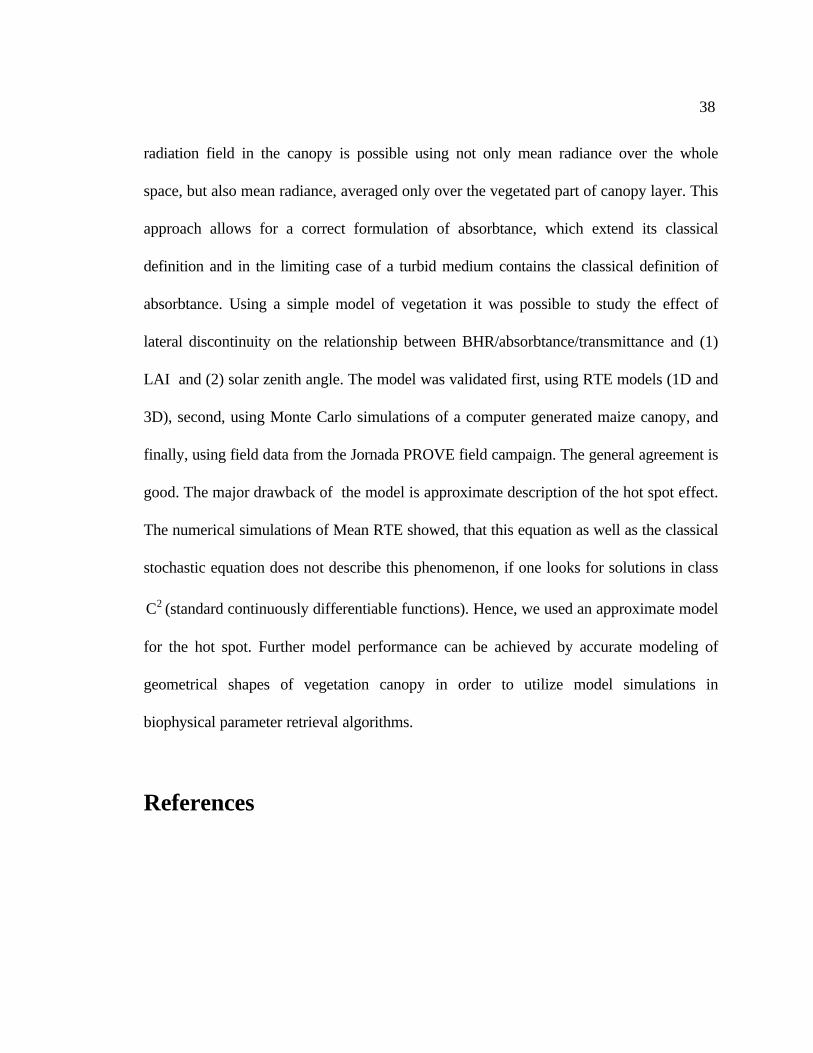
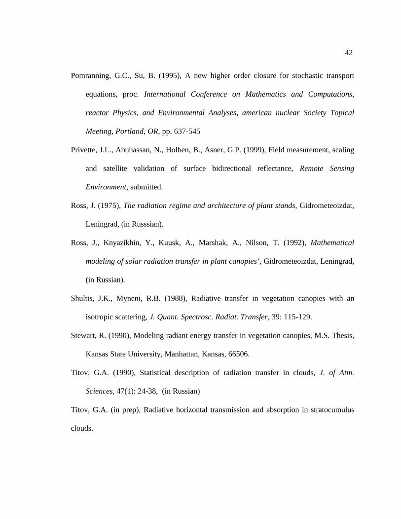
1 The coordinate system with vertical axis z directed down. H is height of ca-

nopy, N- direction to north, ( )ϕθΩ ,&

- is direction, with θ as zenith angle and

ϕ as azimuth angle. ………………………………………………………….… 44

2 Procedure for integration of RTE. Points A and B correspond to the starting

points of integration (located on boundaries), which is performed along the

direction θ up to the inner point C, which has the coordinates (x,y,z). Points

D and F designate any point located on lines AC and BC. The 3D equation

of lines AC and BC is given (the parameter, controling location on the line

is ξ ). ……...……………………………………………………..………………. 45

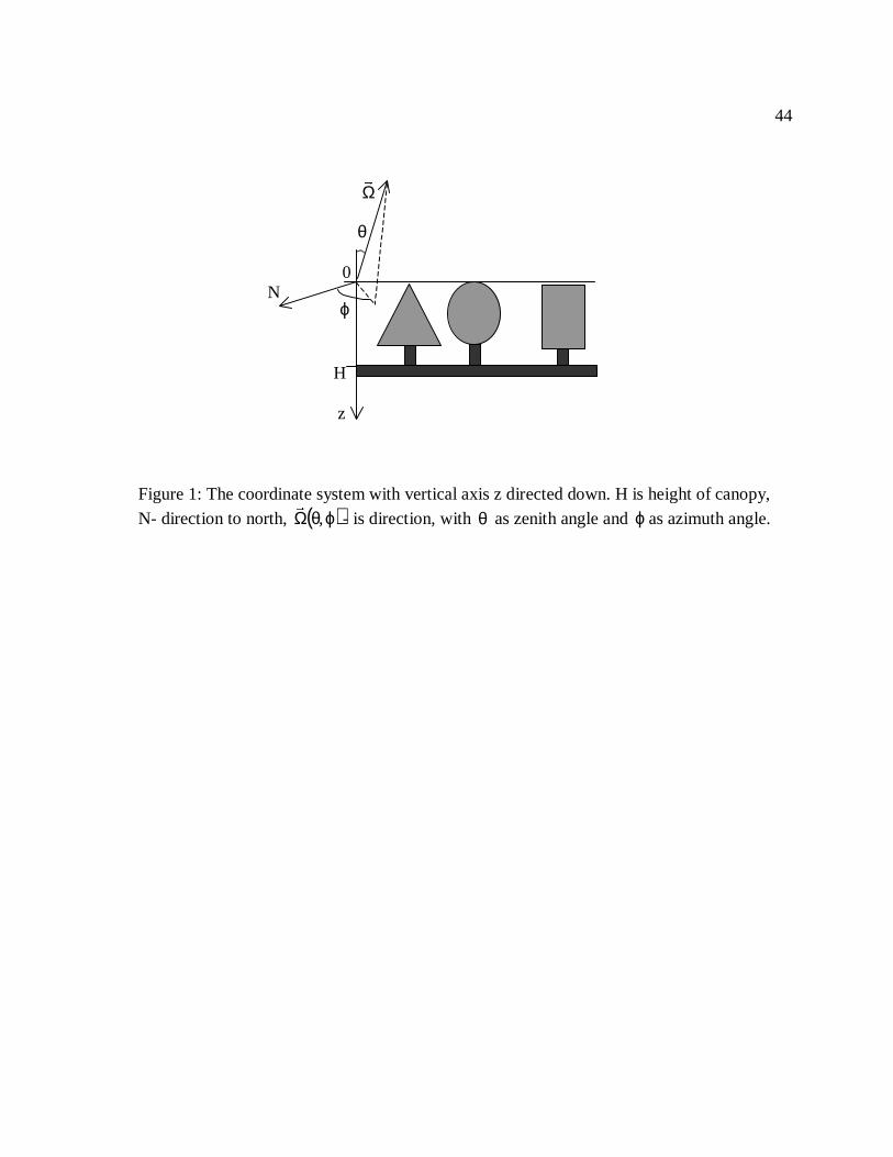
3 Comparison of BRF in the principal plane simulated by Mean RTE (solid line)

and Monte Carlo (dashed line) methods. In all cases soil is “dry”, cab=50

and SZA=45 degrees. ………………………………………………………….… 46

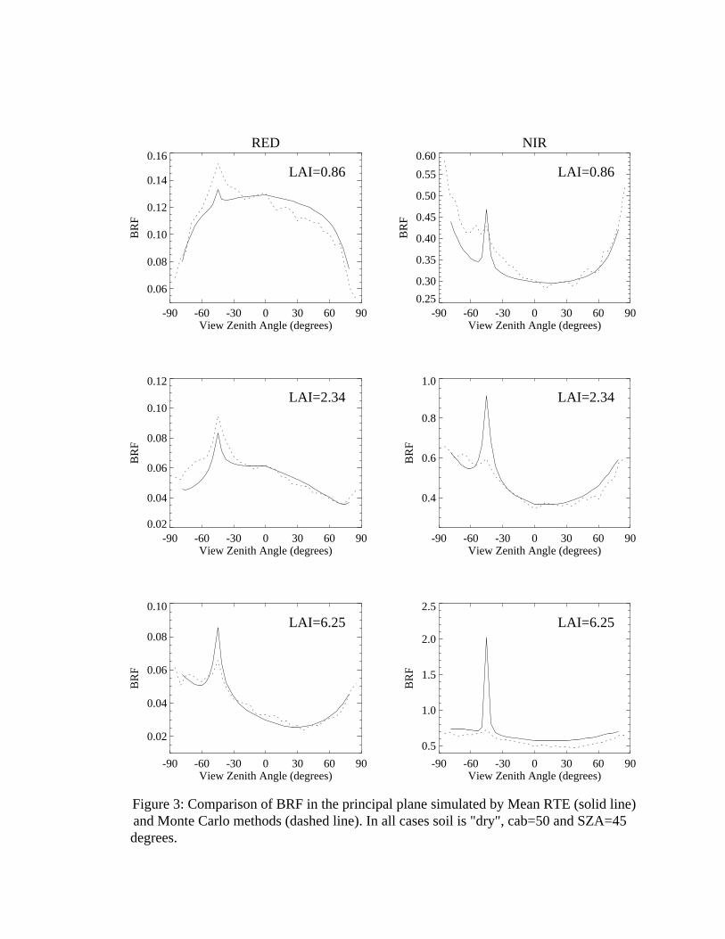
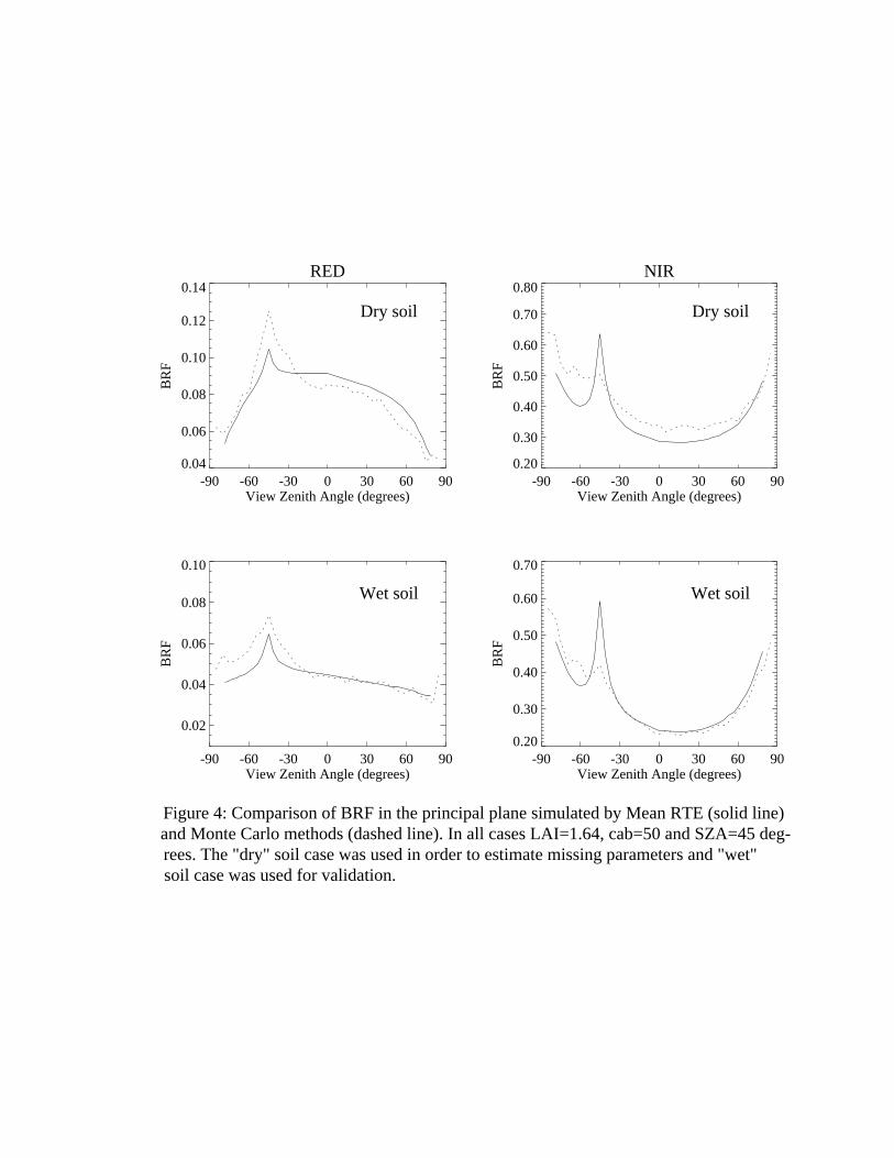
4 Comparison of BRF in the principal plane simulated by Mean RTE (solid

line) and Monte Carlo (dashed line) methods. In all cases LAI=1.64, cab=

50 and SZA=45 degrees. The “dry” soil case was used in order to estimate

missing parameters and “wet” soil case was used for validation. …….…………. 47

5 Comparison of DHR simulated by Mean RTE and Monte Carlo Methods

for “dry” and “wet” soil cases. 50 values of DHR were compared in the case

of “dry” soil and 30 values for “wet” soil. ……………………………….……… 48

viii

6 BHR, absorptance and transmittance as a function of LAI at red (left) and

near-infrared (right) wavelengths evaluated with Mean RTE (solid line),

TWOVEG (dashed line) and DISORD (doted line). In all cases SZA=30

degrees. …………………………………………………………………………… 49

7 BHR, absorptance and transmittance as a function of solar zenith angle at red

(left) and near-infrared (right) wavelengths evaluated with Mean RTE (solid

line), TWOVEG (dashed line) and DISORD (doted line). In all cases LAI=5. … 50

8 Comparison of BRF simulated by Mean RTE with Jornada PROVE field data

at 1020 nm and 870 nm for 3 values of SZA: 20, 40 and 70 degrees. …………... 51

9 Influence of clumping on the radiation regime in vegetation canopy at red

(left) and near-infrared (right) wavelengths. BHR, absorptance and transmit-

tance as a function of LAI evaluated at three values of ground cover, repre-

senting varying degree of clumping: P=1.0 (dashed line), P=0.75 (doted line),

P=0.5 (solid line). In all cases SZA=30 degrees. …………………………...…… 52

10 Influence of clumping on radiation regime in vegetation canopy at red (left)

and near-infrared (right) wavelengths. BHR, asorptance and transmittance

as a function of solar zenith angle evaluated at 3 values of ground cover,

representing, representing varying degree of clumping: P=1.0 (dashed line),

P=0.75 (doted line), P=0.5 (solid line). In all cases LAI=5. ……………………. 53

ix

List of Abbreviations

H- total depth (height) of canopy

zyx ,, ΩΩΩ=Ω&

- unit vector

0Ω&

- direction of direct solar radiation

( )Ωµ&

- cosine of polar angle of Ω&

)( 0Ω−Ωδ&&

- Dirac delta function

z,y,xr =&

- coordinate triplet

)r(&

χ - indicator function

),r(I Ω&

&

- radiance (intensity) at spatial point r&

and in direction Ω&

),z(I Ω&

- mean radiance, averaged over the horizontal plane at depth z

),z(U Ω&

- mean radiance, averaged over the vegetated portion of a horizontal plane z

( )00R y,xS - cylinder of height H, with vertical axis located at point( )00 y,x and radius R

zT - area of horizontal plane z, [ ]H;0z∈ covered by vegetation

( )00z y,xT - manifold zT , shifted by vector 00 y,x

zR TS ∩ - common area of manifold RS , zT

)S(Mes - measure of area S

)z(p - horizontal density of vegetation (HDV) at level z

)r(uL

&

- foliage area volume density (FAVD), [ 32 m/m ]

λ - wavelength

x

)(rD λ - spectral hemispherical reflectance of the leaf

)(tD λ - spectral hemispherical transmittance of the leaf

)(λω - single-scattering leaf albedo

)(soil λρ - soil hemispherical reflectance

),r(G Ω&

&

- mean projection of leaf normals in the direction Ω&

),r(1 Ω→Ω′Γπ&&

&

- area scattering phase function

)(S Ω→Ω′σ&&

- differential scattering cross-section

)(Ωσ&

- extinction coefficient

HDRF- the Hemispherical-Directional Reflectance Factor

BHR- the Bi-Hemispherical Reflectance

1

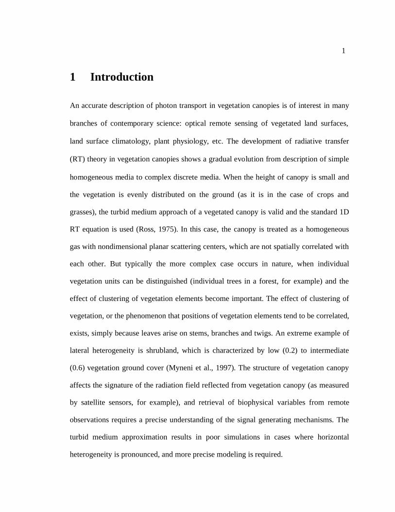
1 Introduction

An accurate description of photon transport in vegetation canopies is of interest in many

branches of contemporary science: optical remote sensing of vegetated land surfaces,

land surface climatology, plant physiology, etc. The development of radiative transfer

(RT) theory in vegetation canopies shows a gradual evolution from description of simple

homogeneous media to complex discrete media. When the height of canopy is small and

the vegetation is evenly distributed on the ground (as it is in the case of crops and

grasses), the turbid medium approach of a vegetated canopy is valid and the standard 1D

RT equation is used (Ross, 1975). In this case, the canopy is treated as a homogeneous

gas with nondimensional planar scattering centers, which are not spatially correlated with

each other. But typically the more complex case occurs in nature, when individual

vegetation units can be distinguished (individual trees in a forest, for example) and the

effect of clustering of vegetation elements become important. The effect of clustering of

vegetation, or the phenomenon that positions of vegetation elements tend to be correlated,

exists, simply because leaves arise on stems, branches and twigs. An extreme example of

lateral heterogeneity is shrubland, which is characterized by low (0.2) to intermediate

(0.6) vegetation ground cover (Myneni et al., 1997). The structure of vegetation canopy

affects the signature of the radiation field reflected from vegetation canopy (as measured

by satellite sensors, for example), and retrieval of biophysical variables from remote

observations requires a precise understanding of the signal generating mechanisms. The

turbid medium approximation results in poor simulations in cases where horizontal

heterogeneity is pronounced, and more precise modeling is required.

2

The notion of gaps (or voids) between canopy clusters must be introduced along

with precise description of topology of the boundary of vegetation in order to describe the

signature of radiation field in discontinuous canopy. Nilson (1991), later Li and Strahler

(1992), introduced a geometrical-optical approach to calculate the reflected radiance from

such vegetation boundaries. They use the notion of mutual shadowing (vegetation unit

casting shadows on such units) and Bidirectional Gap Probability (probability of sensing

radiation reflected by vegetation along the direction Ω&

, if it was illuminated by solar

radiation along 0Ω&

), to describe the boundary of vegetation. This approach allows an

explanation for the hot-spot effect (the peak in reflected radiance distribution along the

retro-illumination direction, due to the absence of shadows in this direction). The

approach is valid in the visible part of solar spectrum, where one can restrict the study of

radiation interaction to that scattered once from the boundary only. But in the NIR region,

leaf absorption is weak and scattering dominates, and the approach of Nilson/Li and

Strahler is not accurate. The problem lies in an accurate description of multiple

scattering, and propagation of radiation into deeper parts of the canopy. Currently only

the Monte Carlo method (Marshak, Ross, 1991) works well at all wavelengths, but this

method has a several disadvantages: these include computational expense, difficulty to

adopt to user specific needs, and lack of analytical analysis.

Another analytical approach describing leaf clumping in vegetation canopies is

the statistical approach. Of importance is the problem of deriving analytical expressions

or equations for moments which characterize the stochastic radiative field in a vegetation

canopy. The most critical is the expression for the first moment of the radiation field, the

3

mean intensity. The problem of investigating the stochastic equations for the mean field

has been a highly active research field in recent years (Pomraning, 1995). The first

significant attempt to apply statistical approach to describe vegetation canopy was made

by Menzhulin and Anisimov (1991). A more manageable closed system of statistical

equations for the mean intensity was derived in applications to a medium of broken

clouds, initially by Vainikko (1973a, 1973b) and later by Titov (1990), and Zuev and

Titov (1996). This approach can be applied to vegetation canopies but with some

modifications.

In this thesis, an exact stochastic radiative transfer equation for the mean

intensity in a discontinuous vegetation canopy is derived. This equation is based on the

work of Vainikko (1973a) for broken clouds together with classical parameters of a

vegetation canopy originally introduced by Ross (1975). We obtained a system of

integral equations, which were solved numerically. The simulated radiation regime in a

discontinuous canopy was validated in several ways, including comparison with field

data from Jornada PROVE (Privette et al., 1999).

This thesis is organized as follows. In Section 2 we review the basic concepts of

radiative transfer in vegetation media and introduce the classical stochastic 3-dimensional

radiative transfer equation with the corresponding boundary conditions. The derivation of

the transfer equation for the mean field using a statistical approach is described in Section

3. Issues resulting from the effect of discontinuity in vegetated media and analytical

description of this discontinuity (in particular, a new formula for absorptance) are

discussed in Section 4. In section 5, a numerical method for solving the transfer equation

4

for the mean field is outlined and issues related to speed of convergence are presented.

Section 6 presents detailed description of important outputs of the model and

comparisons with output from similar RTE models, radiation field in Maize canopy

simulated using Monte Carlo method and field data from Jornada PROVE. In addition, a

numerical study of the effect of discontinuity on the radiation field in a vegetation canopy

presented.

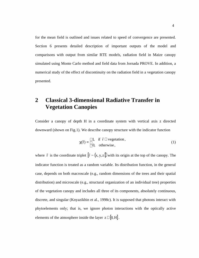
2 Classical 3-dimensional Radiative Transfer inVegetation Canopies

Consider a canopy of depth H in a coordinate system with vertical axis z directed

downward (shown on Fig.1). We describe canopy structure with the indicator function

∈

=χ,otherwise,0

,vegetationrif,1)r(

&

&

(1)

where r&

is the coordinate triplet ( )[ ]z,y,x~r&

with its origin at the top of the canopy. The

indicator function is treated as a random variable. Its distribution function, in the general

case, depends on both macroscale (e.g., random dimensions of the trees and their spatial

distribution) and microscale (e.g., structural organization of an individual tree) properties

of the vegetation canopy and includes all three of its components, absolutely continuous,

discrete, and singular (Knyazikhin et al., 1998c). It is supposed that photons interact with

phytoelements only; that is, we ignore photon interactions with the optically active

elements of the atmosphere inside the layer [ ]H,0z∈ .

5

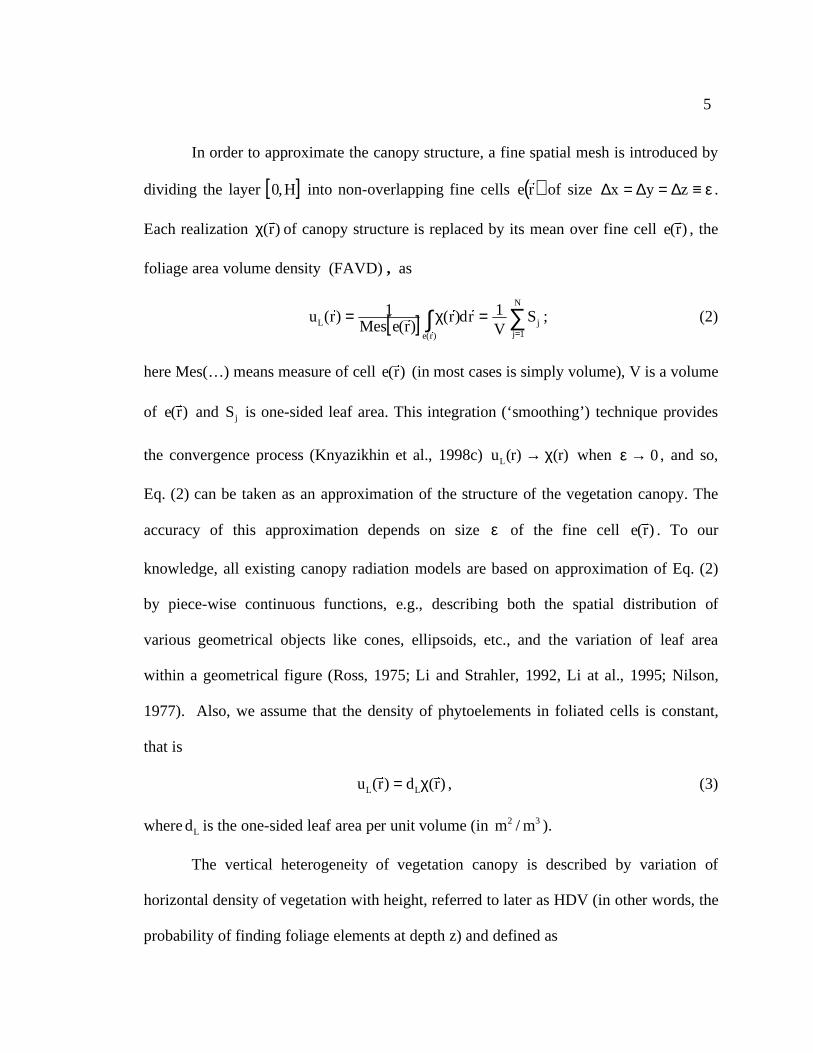
In order to approximate the canopy structure, a fine spatial mesh is introduced by

dividing the layer[ ]H,0 into non-overlapping fine cells ( )re&

of size ε≡∆=∆=∆ zyx .

Each realization )r(&

χ of canopy structure is replaced by its mean over fine cell )r(e&

, the

foliage area volume density (FAVD) , as

[ ] =χ= ∫)r(e

L rd)r()r(eMes

1)r(u&

&&

&

& ∑=

N

1jjS

V1 ; (2)

here Mes(…) means measure of cell )r(e&

(in most cases is simply volume), V is a volume

of )r(e&

and jS is one-sided leaf area. This integration (‘smoothing’) technique provides

the convergence process (Knyazikhin et al., 1998c) )r()r(uL χ→ when 0→ε , and so,

Eq. (2) can be taken as an approximation of the structure of the vegetation canopy. The

accuracy of this approximation depends on size ε of the fine cell )r(e&

. To our

knowledge, all existing canopy radiation models are based on approximation of Eq. (2)

by piece-wise continuous functions, e.g., describing both the spatial distribution of

various geometrical objects like cones, ellipsoids, etc., and the variation of leaf area

within a geometrical figure (Ross, 1975; Li and Strahler, 1992, Li at al., 1995; Nilson,

1977). Also, we assume that the density of phytoelements in foliated cells is constant,

that is

)r(d)r(u LL

&&

χ= , (3)

where Ld is the one-sided leaf area per unit volume (in 32 m/m ).

The vertical heterogeneity of vegetation canopy is described by variation of

horizontal density of vegetation with height, referred to later as HDV (in other words, the

probability of finding foliage elements at depth z) and defined as

6

;dydx)r(S

1)z(p

y,x∫∫ χ= &

(4)

here S means sufficiently large area over the horizontal plane z. In terms of these notati-

ons, the leaf area index (LAI) can be expressed as

.d)(pddydx)r(S1dddV)r(

Sd

dV)r(uS1LAI

H

0

L

y,x

H

0

L

V

L

V

L ∫∫∫∫∫∫ ξξ=χξ=χ==&&&

(5)

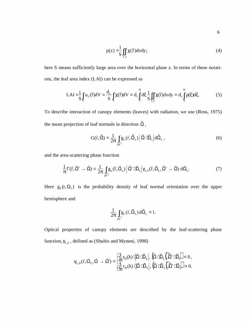
To describe interaction of canopy elements (leaves) with radiation, we use (Ross, 1975)

the mean projection of leaf normals in direction Ω&

,

,d),r(g21),r(G L

2

LLL ΩΩ⋅ΩΩπ=Ω ∫+π

&&&&

&

&

&

(6)

and the area-scattering phase function

.d),,r(),r(g21),r(1

LL,L

2

LLL ΩΩ→Ω′ΩγΩ⋅Ω′Ωπ=Ω→Ω′Γπ λ+π∫

&&&&

&

&&&

&

&&

&

(7)

Here ),r(g LL Ω is the probability density of leaf normal orientation over the upper

hemisphere and

.1d),r(g21

L

2

LL =ΩΩπ ∫+π

&&

&

Optical properties of canopy elements are described by the leaf-scattering phase

function, λγ ,L , defined as (Shultis and Myneni, 1998)

( )( )( )( )

>Ω⋅Ω′Ω⋅ΩΩ⋅Ω⋅λπ

<Ω⋅Ω′Ω⋅ΩΩ⋅Ω⋅λπ=Ω′→ΩΩγ λ.0,)(t1

,0,)(r1),,r(

LLLD

LLLDL,L &&&&&&

&&&&&&

&&&

&

7

Here )(rD λ and )(tD λ are the spectral hemispherical reflectance and transmittance,

respectively, of the leaf element. The leaf scattering phase function integrated over all

exit photon directions yields the single-scattering leaf albedo (per unit leaf area), )(λω ,

i.e.,

)(d),,r(4

L,L λω=Ω′Ω′→ΩΩγ∫π

λ

&&&&

&

.

With this background information, we can compactly represent the extinction

coefficient )(Ωσ&

and the differential scattering coefficient )(S Ω→Ω′σ&&

as (Ross, 1975)

),r(ˆ)r()(),r(G)r(d),r(G)r(u LL Ωσ=χΩσ=Ωχ=Ω&

&&

&&

&&

&

&&

, (8)

and,

),r(ˆ)r()(),r()r(d

),r()r(u

SSLL Ω→Ω′σ=χΩ→Ω′σ=Ω→Ω′Γπχ=Ω→Ω′Γ

π

&&

&&

&&&&

&

&

&&

&

&

. (9)

The radiation regime in such a canopy is described by the transport equation (Knyazikhin

et al., 1998b)

.d),r(I)()r(),r(I)()r(),r(I4

S Ω′Ω′Ω→Ω′σχ=ΩΩσχ+Ω∇⋅Ω ∫π

&&

&

&&

&

&

&

&

&

&

&

&

(10)

This equation will be referred later as the classical stochastic radiative transfer equation.

It differs from non-stochastic [introduced for turbid media by Ross (1975)] by the

indicator function )r(&

χ , which modifies the second and third term of Eq. (10).

An important feature of the radiation regime in vegetation canopies is the hot-spot

effect, which is the peak in reflected radiance distribution along the retro-illumination

direction. The standard theory describes the hot-spot by modifying the extinction

coefficient ,)(Ωσ namely (Marshak, 1989),

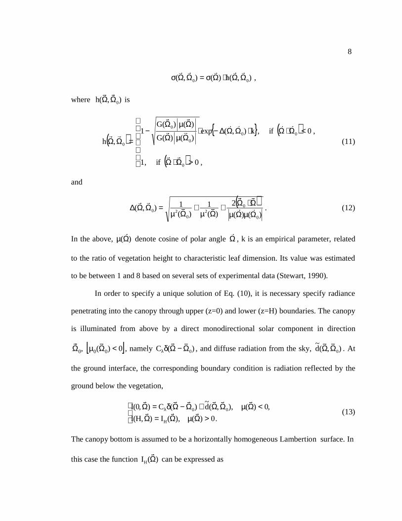
8

),(h)(),( 00 ΩΩ⋅Ωσ=ΩΩσ&&&&&

,

where ),(h 0ΩΩ&&

is

( ) ( )

( )

>Ω⋅Ω

<Ω⋅Ω⋅ΩΩ∆−⋅ΩµΩ

ΩµΩ−

=ΩΩ

,0if,1

,0if,k),(exp)()(G

)()(G1

,h

0

00

0

0

0

&&

&&&&

&&

&&

&&

(11)

and

( ))()(

2)(

1)(

1),(0

02

020 ΩµΩµ

Ω⋅Ω+Ωµ

+Ωµ

=ΩΩ∆ &&

&&

&&

&&

. (12)

In the above, )(Ωµ&

denote cosine of polar angle Ω&

, k is an empirical parameter, related

to the ratio of vegetation height to characteristic leaf dimension. Its value was estimated

to be between 1 and 8 based on several sets of experimental data (Stewart, 1990).

In order to specify a unique solution of Eq. (10), it is necessary specify radiance

penetrating into the canopy through upper (z=0) and lower (z=H) boundaries. The canopy

is illuminated from above by a direct monodirectional solar component in direction

[ ]0)(, 000 <ΩµΩ&&

, namely )(C 0Ω−Ωδλ

&&

, and diffuse radiation from the sky, ),(d~

0ΩΩ&&

. At

the ground interface, the corresponding boundary condition is radiation reflected by the

ground below the vegetation,

>ΩµΩ=Ω<ΩµΩΩ+Ω−Ωδ=Ω λ

.0)(),(I),H(I

,0)(),,(d~

)(C),0(I

H

00&&&

&&&&&&

(13)

The canopy bottom is assumed to be a horizontally homogeneous Lambertion surface. In

this case the function )(IH Ω&

can be expressed as

9

ΩΩµΩπλρ=Ω ∫

−π

&&&&

d)(),H(I)(

)(I2

soilH ,

where )(soil λρ is the soil hemispherical reflectance.

The incoming radiation can be parameterized in terms of two scalar values:

( )0F Ωλ&

, total flux defined as

ΩΩµΩΩ+Ω−Ωδ=ΩΩµΩ≡Ω ∫∫−− π

λπ

λ

&&&&&

d)(),(d~

)(Cd)(),0(I)(F2

00

2

0

,d)(),(d~

)(C2

00 ΩΩµΩΩ+Ωµ= ∫−π

λ

&&&&&

(14)

and )(fdir λ , the ratio of direct radiation incident on the top of plant canopy to the total

incident irradiance

( ) [ ].1;0)(F

)(Cf

0

0

dir ∈Ω

Ωµ≡λ

λ

λ&

&

(15)

Equation (14) and Eq. (15) explain the following formula for incoming solar radiation

[ ] .),(d)(f1)()(

)(f)(F),(d

~)(C 0dir0

0

dir000

ΩΩλ−+Ω−ΩδΩµ

λΩ≡ΩΩ+Ω−Ωδ λλ

&&&&

&

&&&&&

(16)

The general boundary value problem [Eq. (10) and Eq. (13)] can be split into two

simpler sub-problems- (1) Black Soil (BS) problem. In this case all energy input is from

solar radiation (direct and diffuse) and lower boundary (z=H) is assumed to 100%

absorbing . The problem is defined by Eq. (10) and the boundary condition,

10

[ ]

>Ωµ=Ω

<Ωµ

ΩΩλ−+Ω−ΩδΩµ

λΩ=Ω λ

.0)(,0),H(I

,0)(,),(d)(f1)()(

)(f)(F),0(I 0dir0

0

dir0

&&

&&&&&

&

&&

(17)

The solution of BS problem is referred to later as ),r(IBS Ωλ

&

; ),r(IBS Ωλ

&

depends on sun-

view geometry, canopy architecture, and spectral properties of the leaves. (2) Soil (S)

problem. In this case there is no input of energy from above, but the source intensity

),H(I Ω&

is located at the bottom of the canopy. In the case of Lambertian surface

π=Ω /1),H(I&

. The S-problem is defined by Eq. (10) and the boundary condition,

>Ωµπ=Ω<Ωµ=Ω

.0)(,1),H(I

,0)(,0),0(I&&

&&

(18)

Similarly, the solution of S problem is referred to later as ),r(IS Ωλ

&

; ),r(IS Ωλ

&

depends on

spectral properties of leaves and canopy structure only.

After the solutions of ‘BS’ and ‘S’ problems are obtained, one can construct the

solution for the corresponding general case using the following approximations

(Knyazikhin et al., 1998b):

for intensity,

)(F),r(I)(T)(R)(1

)(),r(I),r(I 0

SBS

Ssoil

soilBS Ω⋅

Ω⋅λ⋅λ⋅λρ−

λρ+Ω≈Ω λλλλ

&&&&

, (19)

for reflectance (albedo),

)(T)(T)(R)(1

)()(R)(R SBS

Ssoil

soilBS λ⋅λ⋅

λ⋅λρ−λρ+λ≈λ , (20)

for absorbtance,

11

)(A)(T)(R)(1

)()(A)(A SBS

Ssoil

soilBS λ⋅λ⋅

λ⋅λρ−λρ+λ≈λ , (21)

and transmittance

)(R)(T)(R)(1

)()(T)(T SBS

Ssoil

soilBS λ⋅λ⋅

λ⋅λρ−λρ+λ≈λ , (22)

where )(Ri λ , )(Ti λ , )(Ai λ are the hemispherical reflectance, transmittance and

absorbtance for corresponding ‘i’ problem (i=’S’ or ‘BS’ problem) (cf. Section 4 ).

3 Transfer Equation for the Mean Intensity

The motivation to find mean intensity of solar radiation interacting with vegetation

canopy is simple: sensors aboard satellite platforms measure the mean field emanating

from smallest area to be resolved, a pixel. One possible modeling approach to this

problem is to generate a set of stochastic realizations of vegetation canopies, solve the

classical stochastic RTE [Eq. (10)] and average the solutions. A highly desirable

alternative to this computationally intensive process is to derive a transport equation for

the mean field directly. This problem has been a highly active research field in recent

years (Pomraning, 1995). As mentioned previously the closed system of equations,

12

describing mean intensity of radiation was developed for broken clouds by Vainikko

(1973a, 1973b) and it can be applied to vegetation canopies.

In this section, we will use Vainikko’s approach to derive the equations for mean

radiation intensity in a vegetation canopy. We are interested in two kinds of mean

intensities: (1) the mean intensity over vegetated area, at the level z ]H,0[∈ ,

( ) ( )∫∫∩∞→

Ω∩

=ΩzTRSzRR

dxdy,z,y,xITSMes

1),z(U limrr

(23)

where zT is part of horizontal plane z covered by vegetation and ( )zR TSMes ∩ means area

of plane z covered by vegetation which is inside a circle RS defined at the same plane; and

(2) the mean intensity over total space, at the level z ]H,0[∈ ,

( )∫∫ Ωπ

=Ω∞→ RS

2R

dxdy,z,y,xIR1),z(I lim

rr. (24)

The following important property of stochastic intensity ),r(I Ωr

is valid

( )( ) ( )( )

dxdy,z,y,xIy,xTTSMes

1),z(U1y,1xTzTRS11zRR

lim ∫∫ξ∩∩ξ∞→

Ω∩∩

=Ωrr

, (25)

which simply means that manifold )yx(TT 1,1z ξ∩ contains the same percentage of

vegetation as the total manifold zT . This is the so called assumption of “local chaotisity

and global order” (Vainikko, 1973a).

The procedure to derive the transfer equation for mean intensity from the classical

approach is as follows: First, the classical stochastic transfer equation is integrated from

boundaries ( )Hzand0z == to the some inner point [ ]H,0z ∈ , in order to obtain a linear

integral equation, which still describes a particular random realization of vegetated

13

elements. Second, the transfer equation is averaged over the whole plane z to derive a

formula for ),z(I Ω , which is the mean intensity over the whole horizontal plane. The

equation for ),z(I Ω depends on and is expressed through ),z(U Ω ,

),...],z(U[f),z(I Ω=Ωrr

.

Third, the transfer equation is averaged over part of a horizontal plane z, which is covered

by vegetation [ ]1)r( =χr

, in order to derive the system for unknown ),z(U Ω , mean

radiance over the vegetated portion of the plane.

The averaging procedure, as a general rule, results in equations, which contain

some parameters descriptive of characteristic moments of the media (correlation function

and mean value). The equations for ),z(I Ω and ),z(U Ω depend on the following mean

statistical functions, which must be obtained through corresponding procedure of

modeling the vegetation,

( ) ( ),

R

z,zTTSMes

lim),,z(q 2

z

y

z

xzR

R π

ξ−

ΩΩ

ξ−ΩΩ∩∩

=Ωξξ

∞→

r

which is the probability of finding simultaneously vegetation elements at locations

)z,y,x(M1 and ),,(M2 ξηµ along the direction Ωr

. In the above,

( ) ( )

ξ−

ΩΩ

ξ−ΩΩ∩∩ ξ z,zTTSMes

z

y

z

xzR ,

14

indicates the part of vegetation located on a horizontal plane at depth z that overlaps with

vegetation located on a horizontal plane at depth ξ , if the two planes are moved towards

one another along Ωr

, while keeping them parallel until they collapse. Further,

2

zR

R RTSMes

lim)z(pπ

∩=∞→

(26)

is the probability of finding foliage elements at depth z, or HDV [as defined earlier at Eq.

(4)]. And,

)z(p),,z(q

),,z(KΩξ=Ωξv

r (27)

is the conditional probability of finding a vegetation element at point ),,(M2 ξηµ , which is

located along the direction Ω from )z,y,x(M1 in the plane ξ given )z,y,x(M1 ∈

vegetation.

The detailed procedure to derive the mean RTE is as follows [we follow the

procedure of Vainikko (1973a)]. We start with Eq. (10) and rewrite it in the form,

),z,y,x(gz

),z,y,x(Iy

),z,y,x(Ix

),z,y,x(Izyx Ω=

∂Ω∂Ω+

∂Ω∂Ω+

∂Ω∂Ω

rrrr

, (28)

where the following notation was used

Ω′Ω′Ω→Ω′σχ+ΩΩσχ−≡Ω ∫π

rrrvrrrrrrrd),r(I)()r(),r(I)()r(),z,y,x(g

4

S , (29)

Integration of Eq. (28) from boundaries (z=0 and z=H) to some inner point

( ) [ ]H,0z,z,y,x~r ∈r

along the direction Ωr

(Fig. 2) results in the next system of equations

15

( ) ( )

( ) ( )

>Ωµξ

Ωξξ−ΩΩ

+ξ−ΩΩ+

Ωµ+Ω=Ω

<Ωµξ

Ωξξ−ΩΩ

+ξ−ΩΩ+

Ωµ+Ω=Ω

∫

∫H

z z

y

z

x

z

0 z

y

z

x

.0)(,d,,zy,zxg)(

1),H,y,x(I),z,y,x(I

,0)(,d,,zy,zxg)(

1),0,y,x(I),z,y,x(I(30

)

Inserting formulas for function ),z,y,x(g Ωr

[ ])29(.Eq into Eq. (30), we obtain the

following system:

>ΩΩ+

Ω′Ω′Ω→Ω′σξχΩµ

=ξΩΩσχΩµ

+Ω

<ΩΩ+

Ω′Ω′Ω→Ω′σξχΩµ

=ξΩΩσχΩµ

+Ω

∫ ∫ ∫

∫ ∫ ∫

π

π

.0),,H,y,x(I

d)(...,I)((...)d)(

1d)(...,I)((...))(

1),z,y,x(I

,0),,0,y,x(I

d)(...,I)((...)d)(

1d)(...,I)((...))(

1),z,y,x(I

z

H

z

H

z 4

S

z

z

0

z

0 4

S

r

rrrr

r

rrrr

(31)

where for simplicity the following short cut was introduced

( ) ( ) ξξ−ΩΩ

+ξ−ΩΩ+≡ ,zy,zx...

z

y

z

x (32)

The next step is to average Eq. (31) over the horizontal plane z, [ ]H,0z ∈ . The main

problem is to average item )(...,I(...) Ωχ . It can be done rather straightforwardly after

shifting manifold ξT by vector ( ) ( )

ξ−

ΩΩ

ξ−ΩΩ z,z

z

y

z

x , namely,

( ) ( )

∫∫∫∫

ξ−

Ω

Ωξ−

ΩΩ

ξ∩

=Ωχπ

=Ωχπ

zz

y,z

zxTRS

2

RS2 dxdy)(...,I(...)

R1dxdy)(...,I(...)

R1

( )( ) ∫∫

ξ∩′ξ

ξ ′′Ωξ′′′∩′π

∩′=

TRSR2

R ydxd),,y,x(ITSMes

1R

TSMes,

where

16

( ) ( )

ξ−

ΩΩ

ξ−ΩΩ=′ z,zSS

z

y

z

xRR .

If we recall [ ])26.(Eq ,

2

zR

R RTSMes

lim)z(pπ

∩=∞→

,

we obtain the next limit

),(U)(pdxdy)(...,I(...)R1

RS2

Rlim Ωξ⋅ξ=Ωχ

π ∫∫∞→

. (33)

Keeping in mind Eq.(33) while averaging Eq. (31) over the entire plane z, we finally have

>ΩΩ+

Ω′Ω′ξΩ→Ω′σξξΩµ

=ξΩξξΩσΩµ

+Ω

<ΩΩ+

Ω′Ω′ξΩ→Ω′σξξΩµ

=ξΩξξΩσΩµ

+Ω

∫ ∫ ∫

∫ ∫ ∫

π

π

.0),,H,y,x(I

d),(U)()(pd)(

1d),(U)(p)()(

1),z(I

,0),,0,y,x(I

d),(U)()(pd)(

1d),(U)(p)()(

1),z(I

z

H

z

H

z 4

S

z

z

0

z

0 4

S

r

rrrr

r

rrrr

(34)

The last step is to average the system of Eq.(31) over the portion of horizontal plane z,

[ ]H,0z ∈ , covered by vegetation, zT . Now we need to obtain the value of )(...,I(...) Ωχ

after averaging over zT ,

( ) ( )( ) ( )

∫∫∫∫

ξ−

Ω

Ωξ−

ΩΩ

ξ∩∩∩

=Ωχ∩=Ωχ∩z

z

y,z

zxTzTRS

zRzTRSzR

dxdy)(...,I(...)TSMes

1dxdy)(...,I(...)TSMes

1

( )( ) ( ) ∫∫

ξ∩′∩′ξ

ξ ′′Ωξ′′′∩′π∩

π∩′∩′=

TzTRSR2

zR

2zR ydxd),,y,x(I

TSMes1

R/TSMes

R/TTSMes,

17

where ( ) ( )

ξ−

ΩΩ

ξ−ΩΩ=′ z,zTT

z

y

z

xzz . Taking into account,

( ) ( ) ( )

ξ−

ΩΩ

ξ−ΩΩ∩∩=∩′∩′ ξ z,zTTSMesTTSMes

z

y

z

xzzRzR ,

we obtain

( ) ),(U),,z(Kdxdy)(...,I(...)TSMes

1

RSzRRlim ΩξΩξ=Ωχ

∩ ∫∫∞→

. (35)

Keeping in mind Eq.(35) while averaging Eq. (31) over zT we finally have

>ΩΩ+Ω′Ω′ξΩ→Ω′σ×

ΩξξΩµ

=ξΩξΩξΩσΩµ

+Ω

<ΩΩ+Ω′Ω′ξΩ→Ω′σ×

ΩξξΩµ

=ξΩξΩξΩσΩµ

+Ω

∫∫ ∫

∫∫ ∫

π

π

.0),,H,y,x(Id),(U)(

),,z(Kd)(

1d),(U),,z(K)()(

1),z(U

,0),,0,y,x(Id),(U)(

),,z(Kd)(

1d),(U),,z(K)()(

1),z(U

z

4

S

H

z

H

z

z

4

S

z

0

z

0

rrrrr

rrrrr

(36)

The systems (34) and (36) together form a complete set of equations to determine mean

intensity of radiation in a vegetation canopy.

3.1 Direct and Diffuse Components of ),z(U Ωr

In order to be consistent with boundary conditions [Eq. (13)], the function ),z(U Ω can be

represented as follows

18

,),z(U)()z(U)()(f

)(F

),z(U)(F)()z(UC),z(U

d00

dir0

d00

Ω+Ω−Ωδ

ΩµλΩ≡

≡ΩΩ+Ω−Ωδ=Ω

δλ

λδλ

(37)

where )z(Uδ is the direct component and ),z(Ud Ω is the diffuse component of total mean

intensity over the vegetated area. Inserting Eq. (37) into Eq. (35) we obtain equations for

these two functions. Equation for )z(Uδ , the direct component is

.1d)(U),,z(K)()(

)z(Uz

0

00

0 =ξξΩξΩµΩσ+ δδ ∫ (38)

The system of equations for ),z(Ud Ω , the diffuse components is

[ ]

Ω+ξξΩξΩµΩµ

Ω→Ωσλ=ΩΩ

ΩΩλ−+ξξΩξΩµΩµ

Ω→Ωσλ=ΩΩ

Ω′Ω′ξΩ→Ω′σ=Ωξ>µΩΩ+

ξΩξΩξΩµ

=ξΩξΩξΩµΩσ

+Ω

<µΩΩ+

ξΩξΩξΩµ

=ξΩξΩξΩµΩσ

+Ω

δ

δ

π

∫

∫

∫

∫ ∫

∫ ∫

).(Id)(U),,z(K)()(

)()(f),,z(U

),,(d)(f1d)(U),,z(K)()(

)()(f),,z(U

,d),(U)(),(S:where

,0),,,z(U

d),(S),,z(K)(

1d),(U),,z(K)()(

),z(U

,0),,,z(U

d),(S),,z(K)(

1d),(U),,z(K)()(

),z(U

H

H

z0

0sdir0

dH

0dir

z

00

0sdir0

do

4

ds

0dH

H

z

H

z

dd

0do

z

0

z

0

dd

(39)

3.2 Direct and Diffuse Components of ),z(I Ωr

Similar to the case of ),z(U Ω , the function ),z(I Ω should be consistent with the boundary

condition [Eq.13] and can be represented as follows

19

,),z(I)()z(I)()(f

)(F

),z(I)(F)()z(IC),z(I

d00

dir0

d00

Ω+Ω−Ωδ

ΩµλΩ≡

≡ΩΩ+Ω−Ωδ=Ω

δλ

λδλ

(40)

where )z(Iδ is the direct component and ),z(Id Ω is the diffuse component of total mean

intensity over the total canopy space. Combining Eq. (34) into Eq. (40) we obtain

equations for these functions. The equation for the direct component, )z(Iδ , is

∫ ξξξΩµΩσ−= δδ

z

00

0 d)(U)(p)()(

1)z(I , (41)

The system of equations for ),z(Id Ω , the diffuse component is

[ ]

>µΩ+ξξξΩµΩµ

Ω→Ωσλ=ΩΩ

<µΩΩλ−+ξξξΩµΩµ

Ω→Ωσλ=ΩΩ

Ω′Ω′ξΩ→Ω′σ=Ωξ

>µΩΩ+ΩξξΩµ

+ξΩξξΩµΩσ−=Ω

<µΩΩ+ΩξξΩµ

+ξΩξξΩµΩσ−=Ω

δ

δ

π

∫

∫

∫

∫ ∫

∫ ∫

.0),(Id)(U)(p)()(

)()(f),,z(I

,0),,(d)(f1d)(U)(p)()(

)()(f),,z(I

,d),(U)(),(S:where

,0),,,z(I),(S)(p)(

1d),(U)(p)()(

),z(I

,0),,,z(I),(S)(p)(

1d),(U)(p)()(

),z(I

H

H

z0

0sdir0

dH

0dir

z

00

0sdir0

do

4

ds

H

z

0dH

H

z

dd

z

0

0do

z

0

dd

(42)

It is interesting to note that formula for ),z(I Ω [Eq. (42)] is similar to the system

of equations for ),z(U Ω [Eq. (39)]. The following important property of the equation for

),z(U Ω and ),z(I Ω is valid: if and only if,

),,z(q Ωξ = )(p)z(p ξ⋅ , (43)

which results in

20

)(p)z(p

)(p)z(p)z(p

),,z(q),,z(K ξ=ξ⋅≡Ωξ=Ωξ ,

and then the equations for ),z(U Ω and ),z(I Ω are identical. This means that the mean

intensity over the vegetated area is equal to the mean intensity over the whole space. This

corresponds to the turbid medium case where there is no correlation between the

distribution of vegetated spaces in the canopy.

Another important note about the system of equations for the mean field is: the

equations do not describe the hot spot effect. This is also true for the classical stochastic

equation (Eq. 10). Numerical simulations (described later) atest to this. Thus, we use the

standard approach to implement the hot spot, that is modify the extinction coefficient,

)(Ωσr

.

4 Vegetation Canopy Energy Balance

The results obtained earlier for the mean intensity are necessary for the analysis of energy

fluxes in vegetation canopies. The standard procedure to trace energy input and output

to/from the system is to integrate the equation for the mean intensity [Eq. (42)] over

canopy space and over all directions. The resulting equation describes the energy

conservation law, namely

1T)](1[RA soil =⋅λρ−++ , (general problem) , (44 a)

,1TRA iii =++ (i= BS or S problem), (44 b)

21

where A is absorptance, R is reflectance and T is transmittance for general problem,

defined by Eq. (10) and Eq. (13) or Eq. (39) and Eq (42); iA , iR , iT represent the same,

but for BS and S problems. As mentioned earlier, solution of the general problem can be

expressed through one of BS and S problems [Eq. (19) through Eq. (22)], so we need

only to give the final expressions for iA , iR , iT . In the case of Black Soil problem these

are,

+ΩξΩσξΩξλω−=λ ∫ ∫π

H

0 4

dBS),(U)()(pdd))(1()(A

rrr

ξξξΩµ

Ωσλ+ ∫ δ

H

00

0dir d)(U)(p)(

)()(fr

r

, (45 a)

ΩΩµΩ=λ ∫+π

rrrd)(),0(I)(R

2

dBS , (45 b)

)H(I)(fd)(),H(I)(T dir

2

dBS δ−π

λ+ΩΩµΩ=λ ∫rrr

, (45 c)

and for the Soil problem,

∫∫π

ΩξΩσξΩξλω−=λ4

d

H

0

S ),(U)()(pdd))(1()(Arrr

, (46 a)

ΩΩµΩ=λ ∫−π

rrrd)(),H(I)(R

2

dS , (46 b)

ΩΩµΩ=λ ∫+π

rrrd)(),0(I)(T

2

dS . (46 c)

Note that absorptance for both problems is different from that of the turbid medium

case, that is, the absorptance is expressed not through mean intensity over the total space,

),z(I Ωr

, but through mean intensity over the vegetated area, ),z(U Ωr

. This is due to the

22

fact that energy can be absorbed only by foliage elements, not by voids between leaves (or

between trees). One can compare this result with that for the turbid medium, taking the

BS problem as an example,

[ ]

[ ] .d)(I)(

)()(f),(I)(dd)(1

),(I)(dd)(1),(I)(ddA

H

0 4

H

00

0dird

H

0 4

H

0 4

a

ξξΩµ

Ωσ⋅λ+ΩξΩσΩξλω−=

=ΩξΩσΩξλω−=ΩξΩσΩξ=

∫ ∫ ∫

∫ ∫∫ ∫

πδ

ππ

r

rrrr

rrrrr

(47)

The new formula for absorptance can be derived starting with its physical definition

.dxdyd)(),y,x,0z(I

drd)()r(),r(I

A

S 2

V 4

∫ ∫

∫ ∫

−π

π

ΩΩµΩ=

ΩΩσχΩ≡ rrr

rrrrr

(48)

Assuming that the incident radiant energy is normalized to unity,

,Rdxdyd)(),y,x,0z(I 2

2R 2

π=ΩΩµΩ=∫ ∫π −π

rr

the correct expression for absorptance is,

=ΩΩσχΩπ

=ΩΩσχΩπ

= ∫ ∫ ∫∫ ∫π ππ

dxdy),r(I)()r(ddzR1drd)()r(),r(I

R1A

H

0 4 2R

2V 4

2

vrrrrrrrrr

),(U()(pdzH

0 4∫

π

ΩΩΩ=

),z(U)z(pdxdy)z,y,x(),z,y,x(IR1lim

RS2R

Ω=χΩπ ∫∫∞→

rr.

23

Finally, the new formulation for absorbtance in the general discontinuous case collapses to

the standard turbid medium definition if,

)(p)z(p

)(p)z(p)z(p

),,z(q),,z(K ξ=ξ⋅=Ωξ≡Ωξ

rr

.

This expresses the absence of correlation between vegetated elements located at z and ξ .

5 Numerical Solution of Mean RTE

In order to solve the system of integral equations for mean intensities ),z(U Ωr

, [Eqs. (38)

and (39)] and ),z(I Ωr

, [Eqs. (41) and (42)], a model of vegetation canopy structure is

required together with a numerical scheme for solution of the corresponding transfer

equations. Important variables in the equations for mean intensities are functions )z(p and

),,z(K Ωξr

, which can be obtained from a model of canopy structure. Note that )z(p is the

probability of finding vegetated area in a horizontal plane at depth ]H;0[z ∈ ; and

),,z(K Ωξr

is the conditional probability of the presence of vegetated areas in planes z and

ξ , where ]H;0[,z ∈ξ . We used a simple model of a vegetation canopy by representing

the plants or trees as parallelepipeds distributed on the ground with probability )H(p .

Further, they do not overlap and all have the same dimensions (height, width and depth),

and )H(pconst)z(p == is equal to the portion of the plane covered by vegetation.

Function ),,z(K Ωξr

was calculated by implementing the definition of ),,z(K Ωξr

[Eq. (27)].

24

In the system of integral equations for ),z(I Ωr

and ),z(U Ωr

[Eqs. (49) and (42)], one needs

to solve only the system for ),z(U Ωr

. The evaluation of ),z(I Ωr

is a straightforward

numerical integration of ),z(U Ωr

. In order to solve the system for ),z(U Ωr

, the method of

successive orders of scattering approximations (SOSA) was used (Myneni et al., 1987).

The n-th approximation to the solution is given by

).,z(J...),z(J),z(J),z(U n21nd Ω++Ω+Ω=Ω

The functions n,...,2,1k),,z(Jk =Ω are the solutions of the system of two independent

equations:

,0),,z(Rd),(J),,z(K)()(

),z(J 1kk

z

0

k <µΩ=ξΩξΩξΩµΩσ+Ω −∫ (49)

,0),,z(Rd),(J),,z(K)()(

),z(J 1kk

H

z

k >µΩ=ξΩξΩξΩµΩσ+Ω −∫ (50)

where

[ ] ,1kwhen,0),,(d)(f1

d),(U),,z(K)()(

)()(fd),(S),,z(K

)(1),z(R

0dir

z

00

0Sdirz

0

kk

≥<µΩΩλ−+

ξΩξΩξΩµΩµ

Ω→Ωσλ+ΩΩξΩξΩµ

=Ω ∫∫ δ

,1kwhen,0),,(I

d),(U),,z(K)()(

)()(fd),(S),,z(K

)(1),z(R

0H

H

z0

0SdirH

z

kk

≥>µΩΩ+

ξΩξΩξΩµΩµ

Ω→Ωσλ+ΩΩξΩξΩµ

=Ω ∫∫ δ

and the source function ),z(S Ω is,

25

∫π

Ω′Ω′Ω→Ω′σ=Ω4

kSk d),z(J)(),z(S .

Note that in order to calculate )0k(),z(R0 =Ω , initially 0),z(S =Ω . The algorithm to

solve the system of equations for ),z(U Ω is as follows: (1) Find ),z(U Ωδ from the

corresponding Volterra equation [ ])38(.Eq ; (2) Set 0),z(S =Ω and evaluate ),z(R0 Ω ; (3)

Solve the Volterra equations [ ])50.(Eqand)49(.Eq with ),z(R0 Ω and find ),z(J1 Ω ; (4)

Evaluate ∫π

Ω′Ω′Ω→Ω′σ=Ω4

1S1 d),z(J)(),z(S with ),z(J1 Ω ; (5) Evaluate ),z(R1 Ω ; (6)

Calculate ),z(J2 Ω ; (7) Repeat the following until ε≤Ω),z(Jn : (a) Evaluate ),z(Sk Ω ; (b)

Calculate ),z(Rk Ω ; (c) Calculate ),z(J 1k Ω+ .

The numerical method used to solve the basic equations is as follows. We start

with the parametric Volterra equation,

),z(Fd),(U),,z(K)()(

),z(Uz

0

Ω=ξΩξΩξΩµΩσ+Ω ∫ . (51)

Here Ω is a parameter of the equation. The corresponding discretization scheme is

),,k(F),j(U),j,k(KW)()(

),k(Ukj

1jj,k Ω=ΩΩ

ΩµΩσ+Ω ∑

=

=

(52)

where j,kW is the weight, which depends on the numerical scheme used for approximating

the integral. Then,

1kwhen),,1(F),1(U =Ω=Ω ,

and when [ ]1N,2k z +∈ ,

26

),,j(U),j,k(KW)()(

),k(F),k(U),k,k(KW)()(

),k(U1kj

1jj,kk,k ΩΩ

ΩµΩσ−Ω=ΩΩ

ΩµΩσ+Ω ∑

−=

=

),k,k(KW)()(

1

),j(U),j,k(KW)()(

),k(F

),k(Uk,k

1kj

1jj,k

ΩΩµΩσ+

ΩΩΩµΩσ−Ω

=Ω⇒∑

−=

= . (53)

Another important method used in this algorithm is the method of nS quadratures

of Carlson (Bass et al., 1986) to evaluate angular integrals. This scheme belongs to the

method of Gauss quadratures. The quadrature is built as follows. The octant is divided

into 8

)2n(n +⋅ parts of equal area,

)2n(n4w0 +⋅π= using latitudes, defined as

2n...,,1,0,

21 =µ=µ

+l

l and longitudes, defined as 1

2n,...,1,0m,

21m,

+−=ϕ=ϕ+

ll

. The

coordinates of the boundaries of each layer are:

[ ])2n(n

)11(2n)22n(1

21 +⋅

±−−⋅+−−=µ±

lll

,

and the coordinates of the centers of layers are

[ ])2n(n

22n1

2

+⋅+−−=µ l

l .

The nodes of quadratures are

( )

+−=

−++−

−π=ϕ

=µ⋅+µ=µ−

,12n,...,2,1m,A1

21A

22n1m2

2

,2n,...,1,0,f

nnm,

21

ll

l

l

lll

and the coefficient nAandf are determined to minimize integral.

27

Generally, about 30 iterations are sufficient to obtain relative accuracy of 310− .

The physical interpretation of the method of successive orders is obvious: the function

),z(Jk Ω is the mean radiance of photons scattered k times. The rate of convergence of this

method, cρ has been defined by Vladimirov (1963), Marchuk and Lebedev (1971) as

( ) n)Hkexp(1II 0cn ⋅η⋅⋅−−=ρ≤− , (54)

where 0k is a certain coefficient and

),z()(

supsup 0S

4Hz0 ΩσΩ→Ωσ=η

π∈Ω<<. (55)

From Eq. (44) it follows that SOSA should be used in the case of small optical depth of

the layer or in case of small η . If 1≈η and the optical depth is large, the method becomes

tedious.

6 Evaluation of the Model

To illustrate the characteristics of the mean RTE model described here, numerical results

of calculations of important quantities, such as directional reflectances (BRF) in the

principal plane, energetic quantities [absorbtance, transmittance, reflectance (DHR/BHR)]

are presented in this section. The input variables of Mean RTE model are: (1) solar

illumination variables: solar angle 0Ωr

and the ratio of direct to total incident flux; (2)

canopy geometry, including height H, and horizontal dimensions of individual vegetation

28

units (trees, shrubs), d; (3) statistical moments of the ensemble of vegetation units,

namely, functions p(z) and ( )Ωξ,,zK defined earlier by Eqs. (26) and (27); (4)

characteristics of leaves; density of leaves )r(uL

r, leaf normal orientation distribution

(uniform, planophile, erectophile, etc.) (Ross, 1975), hemispherical reflectance and

transmittance spectra of leaves )(rD λ , )(tD λ ; and, (5) soil hemispherical reflectance spectra

)(soil λρ . Model outputs are (1) the directional reflectances or the Bi-directional

Reflectance Factors (BRF) defined as the surface-leaving radiance, divided by radiance

from a conservative lambertian reflector under monodirectional illumination (Knyazikhin

et al., 1998a)

∫−π

λ

λ

Ω⋅ΩΩΩπ

ΩΩ=

2

top0top

0top

dn),,r(I/1

),,r(IBRF rrrrrr

rrr

; (56)

(2) absorbtance, transmittance and reflectance. We calculate two types of hemispherical

reflectance, BHR and DHR, defined as follows: The Bi-Hemispherical Reflectance (BHR)

for non-isotropic incident radiation (both direct and diffuse components) is the ratio of the

mean radiant exitance to the incident radiance (Knyazikhin et al., 1998a)

∫

∫

−π

λ

+π

λ

Ω⋅ΩΩΩ

Ω⋅ΩΩΩ

=

2

top0top

2

top0top

dn),,r(I

dn),,r(I

BHR rrrrrr

rrrrrr

, (57)

and the Directional Hemispherical Reflectance (DHR) defined similar to BHR, except that

the incident radiation has only the direct component. Below, we present results of

comparison of the Mean RTE model with other RTE models, Monte Carlo simulations of

29

the radiation field in a maize canopy and field data from the Jornada PROVE campaign.

Issues related to the effect of vegetation clumping on the radiation regime are discussed

later.

The three-dimensional dynamic architecture model of maize proposed

by .aletan~Espa (1999) was utilized for the Monte Carlo simulations. This model allows

description of the maize canopy from emergence to male anthesis. Because maize is

planted in rows, and for each vegetation unit the leaves are obviously clumped around the

stem, the assumption of a random leaf spatial distribution is not valid. The driving

parameter of the model is the phenological stage, which is defined by the number of leaves

produced since emergence and not totally hidden in the top leafy cone. The model

describes the dynamics of dimensions, height, senescence, curvature and insertion angle of

the leaves, as well as the temporal evolution of the stem dimensions. Linear equations

were developed to describe growth of the leaf size, stem diameter with change of leaf

stage and so on. The inputs to the 3D model are- (1) leaf stage (which describes time); (2)

plant density, including seeding pattern (row spacing and orientation, plant spacing); (3)

leaf area cumulated over the fully developed plant, including leaves that senesced, and (4)

final height of the canopy. The maize canopy architecture model was calibrated and

validated with three sets of experiments, two of which were performed in Avignon, France

(INRA-90, plant density of 12, 2mplant −⋅ , canopy measured when the fourteenth leaf

appeared; and INRA-97, plant density of 8.5 2mplant −⋅ , measurements performed at two

phenological stages, namely, 13 and 17 leaves). The third experiment was performed in

30

Alpilles, France (Alpilles-97 plant density of 7 2mplant −⋅ , measurements performed when

the fifteenth leaf was appearing).

The maize canopy was simulated using computer graphic techniques as an

assembly of leaves and stems. Six phenological stages of maize were simulated,

corresponding to LAI values of 0.25, 0.86, 1.64, 2.34, 3.01 and 6.25 (Table 1). The

optical properties of the leaves were determined at three chlorophyll a and b

concentrations, Cab30, Cab50, Cab70, which corresponded to 30, 50, 70

2cmg ⋅µ concentrations of chlorophyll a and b. The optical properties for the case of Cab

50, were used in our validation studies (Table 2).

Dry and wet soils with corresponding optical properties were considered

(Baghdadi, 1998). The soil hemispherical reflectances are given in (Table 2). In order to

validate the Mean RTE method, results of simulation from a Monte Carlo ray tracing

method in a maize canopy were utilized (Baghdadi, 1998; .,aletan~Espa 1999). A total of

three million photons were simulated. The incoming photon beams, corresponding to

direct solar illumination, were constrained to have a constant zenith angle of 045 , and 150

azimuthal directions were simulated (in intervals of 04.2 , where 00 corresponds to the

direction perpendicular to the rows). Each of these 150 directions was simulated using

twenty thousand photons. There were 400,3290360 =× viewing directions (steps of

01 along both the zenith and azimuth). The simulations were carried out at 10 wavelengths:

430, 500, 562, 630, 692, 710, 740, 795, 845, 882 in nanometers.

31

The Mean RTE model was run with the same set of input parameters as the Monte

Carlo model. Figures 3, 4 and 5 present results of comparison. We note that not all of the

parameters required to parameterize the Mean RTE model were available; for example,

ground cover and the horizontal dimensions of maize leaves were not available. Therefore,

these parameters were estimated from description of the maize canopy, or in some cases

interpolated using available data. Figure 3 shows simulations of the BRF in the principal

plane for the case of dry soil, chlorophyll concentration of 50 2cmg ⋅µ (Cab 50) at RED

(630 nm ) and NIR (845 nm ) wavelengths, and for three LAI values - low (LAI=0.86),

intermediate (LAI=2.34) and high (LAI=6.25). Other parameters are listed in Table 1. The

incoming radiation was a monodirectional beam incident at a polar angle of 045 . In Fig. 3,

it can be seen that the characteristic shape of BRF changes dramatically from an inverted

bowl to a bowl shape. This provides an opportunity to validate the Mean RTE model.

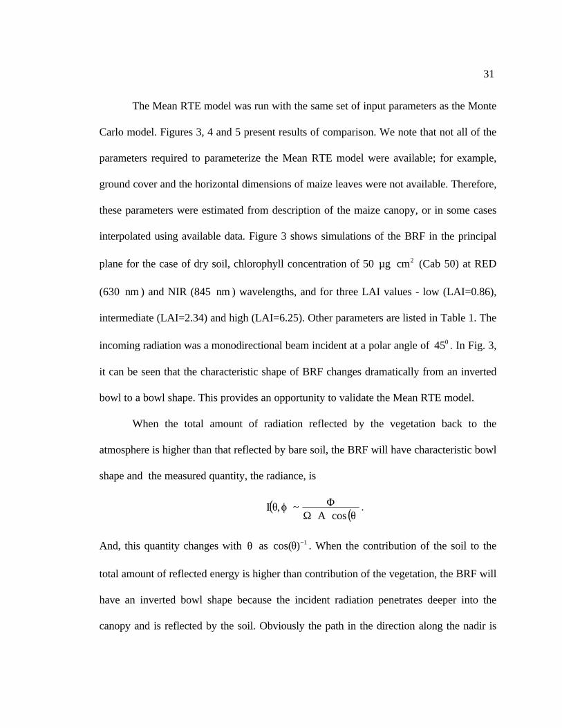
When the total amount of radiation reflected by the vegetation back to the

atmosphere is higher than that reflected by bare soil, the BRF will have characteristic bowl

shape and the measured quantity, the radiance, is

( ) ( )θ⋅⋅ΩΦϕθcosA

~,I .

And, this quantity changes with θ as 1)cos( −θ . When the contribution of the soil to the

total amount of reflected energy is higher than contribution of the vegetation, the BRF will

have an inverted bowl shape because the incident radiation penetrates deeper into the

canopy and is reflected by the soil. Obviously the path in the direction along the nadir is

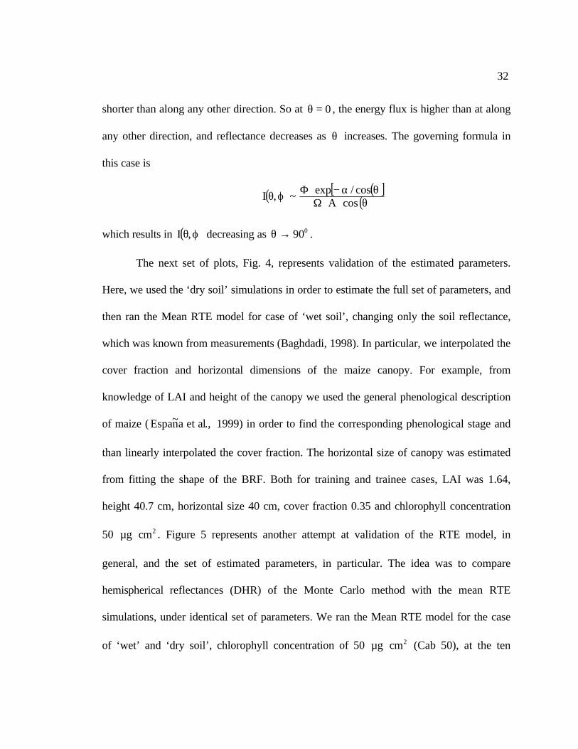
32

shorter than along any other direction. So at 0=θ , the energy flux is higher than at along

any other direction, and reflectance decreases as θ increases. The governing formula in

this case is

( ) ( )[ ]( )θ⋅⋅Ω

θα−⋅ΦϕθcosA

cos/exp~,I

which results in ( )ϕθ,I decreasing as 090→θ .

The next set of plots, Fig. 4, represents validation of the estimated parameters.

Here, we used the ‘dry soil’ simulations in order to estimate the full set of parameters, and

then ran the Mean RTE model for case of ‘wet soil’, changing only the soil reflectance,

which was known from measurements (Baghdadi, 1998). In particular, we interpolated the

cover fraction and horizontal dimensions of the maize canopy. For example, from

knowledge of LAI and height of the canopy we used the general phenological description

of maize ( .,aletan~Espa 1999) in order to find the corresponding phenological stage and

than linearly interpolated the cover fraction. The horizontal size of canopy was estimated

from fitting the shape of the BRF. Both for training and trainee cases, LAI was 1.64,

height 40.7 cm, horizontal size 40 cm, cover fraction 0.35 and chlorophyll concentration

50 2cmg ⋅µ . Figure 5 represents another attempt at validation of the RTE model, in

general, and the set of estimated parameters, in particular. The idea was to compare

hemispherical reflectances (DHR) of the Monte Carlo method with the mean RTE

simulations, under identical set of parameters. We ran the Mean RTE model for the case

of ‘wet’ and ‘dry soil’, chlorophyll concentration of 50 2cmg ⋅µ (Cab 50), at the ten

33

available wavelengths (Table 1). For the case of dry soil, five values of LAI were used

(LAI=0.86; 1.64; 2.34; 3.01; 6.25), and three for the case of wet soil (LAI=1.64; 3.01;

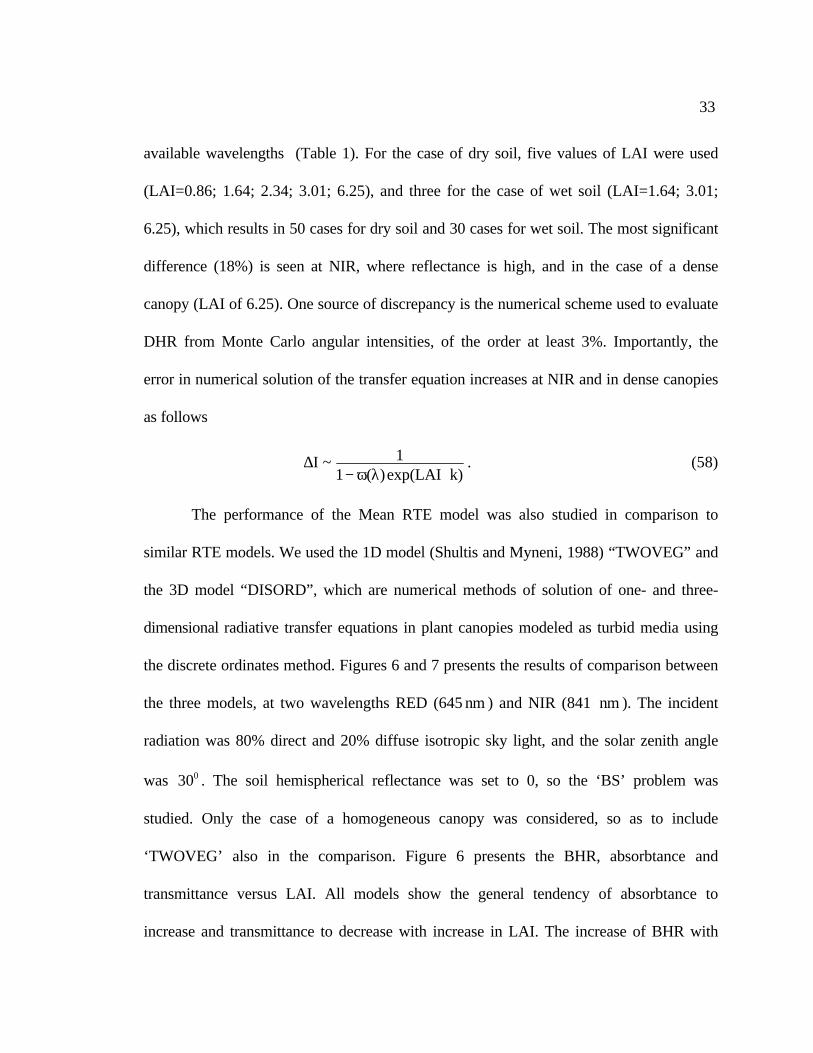
6.25), which results in 50 cases for dry soil and 30 cases for wet soil. The most significant

difference (18%) is seen at NIR, where reflectance is high, and in the case of a dense

canopy (LAI of 6.25). One source of discrepancy is the numerical scheme used to evaluate

DHR from Monte Carlo angular intensities, of the order at least 3%. Importantly, the

error in numerical solution of the transfer equation increases at NIR and in dense canopies

as follows

)kLAIexp()(11~I

⋅λω−∆ . (58)

The performance of the Mean RTE model was also studied in comparison to

similar RTE models. We used the 1D model (Shultis and Myneni, 1988) “TWOVEG” and

the 3D model “DISORD”, which are numerical methods of solution of one- and three-

dimensional radiative transfer equations in plant canopies modeled as turbid media using

the discrete ordinates method. Figures 6 and 7 presents the results of comparison between

the three models, at two wavelengths RED (645 nm ) and NIR (841 nm ). The incident

radiation was 80% direct and 20% diffuse isotropic sky light, and the solar zenith angle

was 030 . The soil hemispherical reflectance was set to 0, so the ‘BS’ problem was

studied. Only the case of a homogeneous canopy was considered, so as to include

‘TWOVEG’ also in the comparison. Figure 6 presents the BHR, absorbtance and

transmittance versus LAI. All models show the general tendency of absorbtance to

increase and transmittance to decrease with increase in LAI. The increase of BHR with

34

LAI is due to the completely absorbing soil, and as LAI increases, the leaves hide this

perfect absorber, and hence the increase in BHR. Figure 7 illustrates dependencies of

BHR, absorbtance and transmittance with respect to solar zenith angle at a constant LAI

of 5. The general tendency of absorbtance to increase, transmittance to decrease with

increase in solar zenith angle is correct, because the pathlength increases as the solar

zenith angle increases and the probability of the solar rays to be intercepted also increases.

Bihemispherical reflectance also increases with increase in solar zenith angle because at

oblique sun angles, more energy is reflected from the boundary and there is

correspondingly less penetration into the deeper parts of the canopy. From Figs. 6 and 7, it

can be seen that the largest discrepancy between model estimates is for BHR, especially

between the Mean RTE and ‘DISORD’ at RED, for absorbtance versus solar zenith angle

at both RED and NIR and, for transmittance versus solar zenith angle at RED, which may

be attributed to various simplifying approximations used in the numerical solution

schemes.

The critical validation of any model is comparison with field data. We utilized data

from the Jornada field campaign, distributed by the grassland PROVE (PROtotype

Validation Exercise) team (Privette et al., 1999). This experiment took place from April

30 through May 13 of 1997 in Jornada (a large valley near Las Cruces, New Mexico,

USA). The area is slowly undergoing a landcover change from a grassland to a shrubland

(predominately mesquite). It is a very arid area, so shrubs and grasses are sparse [ground

cover is )%25.34( ± , average LAI ~0.5]. The data were from a transitional site (mixed

35

grassland and shrubs) and consisted of 75% of mesquite and 25% of yucca and morman

tea. The measurements were performed on a 26 m tall tower using CIMEL sunphotometer

which has 4 channels;- we used data from two of these channels: 870 nm and 1020 nm.

Related parameters at the Jornada transition site are as follows (for Mesquite): mean

height: 54.028.1 ± m, LAI: 1.71, leaf reflectance at 870 nm: 0.432, leaf transmittance at

870 nm: 0.395, leaf reflectance at 1020 nm: 0.442, leaf transmittance at 1020 nm: 0.399.

For Yucca we have: mean height 16.059.0 ± m, LAI: 1.38, leaf reflectance at 870 nm:

0.432, leaf transmittance at 870 nm: 0.107, leaf reflectance at 1020 nm: 0.426, leaf

transmittance at 1020 nm: 0.096. Soil reflectance was 0.349 (at 870 nm), and 0.380 (at

1020 nm). Figure 8 presents BRF comparisons (field data and simulated by the Mean

RTE) in the principal plane for three values of solar zenith angle ( 000 70,40,20 ) and at

two available wavelengths (1020 nm and 870 nm). Because the data were noisy, it is

difficult to perform detailed comparisons, but it appears that the agreement is reasonable.

One exception is the comparison for 870 nm at SZA of 040 , where the simulated BRF is a

significant overestimate. There are indications that the data may have a problem in this

instance (Privette, private communications): from others plots it is clear that the mean

BRF for both channels is approximately the same at a given value of SZA. The plot under

consideration is an exception.

Finally, we discuss one important feature of the Mean RTE model, which allows

for description of canopy heterogeneity, i.e., mixing of voids with clusters of vegetation

elements. The effect of clustering has an important influence on the radiation regime in a

36

vegetation canopy, for example the hot spot effect and change in the proportions of BHR,

absorbtance and transmittance. We already mentioned that heterogeneity leads to a new

analytical formula for absorbtance (Sec.4), for which we must use not the mean intensity

over all space, but the mean intensity over only the vegetated portion of the canopy space

[Eqs. (38) and (39)]. Figures 9 and 10 illustrate the influence of clumping on BHR,

absorbtance and transmittance, for the case of a black soil problem, and for a direct to

total incident flux ratio of 8.0)(fdir =λ . In order to introduce voids, we varied the ground

cover parameter and ran the Mean RTE for p(z)=1.0 (which corresponds to the turbid

medium case), p(z)=0.75 and p(z)=0.5 (as p decreases, clumping increases). Figure 9

presents the relationship between BHR, absorbtance and transmittance with LAI (SZA is

equal to 030 ). Figure 10 presents the same, but with changing solar zenith angle at a

constant LAI of 5. The qualitative effect of voids on the radiation regime is similar at NIR

and RED wavelengths. From Fig. 9 it is clear that for similar input parameters, in

particular LAI, but at different values of ground cover, the BHR and absorbtance decrease

as groundcover decrease, and transmittance increases. The same tendency is observed for

BHR, absorbtance and transmittance versus solar zenith angle (Fig. 10). The above

corresponds to clumping vegetation into clusters, thereby increasing the amount of voids

and the probability of solar radiation to penetrate deeper into the canopy which result in

increased transmittance and decreased absorbtance. The quantitative effect of clumping is,

for example, at LAI=3, SZA= 050 , at RED, ( )0.1pBHRBHR =≡∆ )5.0p(BHR =− /

)0.1p(BHR = %3.42≈ , similarly, ∆ Absorbtance %30≈ and ∆ Transmittance %150≈

37

7 Concluding Remarks

The major goal of this work was to address the problem of accurately describing

the influence of discontinuity in vegetation canopies on the radiative regime. The presence

of gaps in vegetation canopies introduces corrections to energy fluxes compared to values

of fluxes for the homogeneous case and consequently results in large errors in the

retrieved biophysical parameters of vegetation such as LAI, FPAR, etc. Among the many

current models those, based on geometrical-optical approach are valid for discontinuous

vegetation canopies, but they approximate radiative fluxes and multiple scattering of

photons; others, based on the classical RT equation, are accurate but applicable only to

simple homogeneous cases of crops and grasses.

The proposed approach, based on a statistical formulation of Radiative Transfer

Equations, is specially designed to accurately evaluate radiation fluxes in discontinuous

vegetation canopies. Special attention was given to deriving analytical results. More

specifically, the following major tasks were accomplished. A governing integral equation

of the mean field for the transport of monochromatic radiation intensity in spatially

heterogeneous canopy has been formulated. The resulting system of integral equations

satisfies to the energy conservation law and was solved numerically using the method of

successive orders of scattering approximations. The influence of discontinuity on the

radiative regime in a vegetation canopy is such, that, a complete description of the

38

radiation field in the canopy is possible using not only mean radiance over the whole

space, but also mean radiance, averaged only over the vegetated part of canopy layer. This

approach allows for a correct formulation of absorbtance, which extend its classical

definition and in the limiting case of a turbid medium contains the classical definition of

absorbtance. Using a simple model of vegetation it was possible to study the effect of

lateral discontinuity on the relationship between BHR/absorbtance/transmittance and (1)

LAI and (2) solar zenith angle. The model was validated first, using RTE models (1D and

3D), second, using Monte Carlo simulations of a computer generated maize canopy, and

finally, using field data from the Jornada PROVE field campaign. The general agreement is

good. The major drawback of the model is approximate description of the hot spot effect.

The numerical simulations of Mean RTE showed, that this equation as well as the classical

stochastic equation does not describe this phenomenon, if one looks for solutions in class

2C (standard continuously differentiable functions). Hence, we used an approximate model

for the hot spot. Further model performance can be achieved by accurate modeling of

geometrical shapes of vegetation canopy in order to utilize model simulations in

biophysical parameter retrieval algorithms.

References

39

Baghdadi, N., Baret, F. (1998), Amelioration du modele de transfert radiatif SAIL a

partur D’Un modele de lancer de rayons: cas du mais. Rapport D’active, INRA,

Avignon (in French).

Bass, L.P., Voloschenko, A.M., Germogenova, T.A. (1986), Methods of discrete

ordinates in radiation transport problems, Institute of applied mathematics,

Moscow, pp. 21-23, (in Russian).

Diner, D.J., Martonchik, J.V., Borel, C., Gerstl, S.A.W., Gordon, H.R. Knyazikhin, Y.,

Myneni, R., Pinty, B. and Verstrate, M.M. (1998a), MISR: Level 2 surface retrieval

algorithm theoretical basis, JPL Internal Document D-11401, Rev. C, California

Institute of Technology, Jet Propulsion Laboratory, Pasadena.

Diner, D.J., Abdou, W.A., Gordon, H.R., Kahn, R.A., Knyazikhin, Y., Martonchik, J.V.

McMuldroch, S., Myneni, R., West, R.A. (1998b), Level 2 ancillary products and

datasets Algorithm theoretical basis, JPL Internal Document D-13402, Rev. A,

California Institute of Technology, Jet Propulsion Laboratory, Pasadena.

an~Espa , M., Baret, F., Chelle, M., Aries, F., Bruno, A., (in press), A dynamic model of

maize 3D architecture: application to the parameterisation of the clumpiness of the

canopy, Agronomie.

Jupp, D. L. B., Strahler, A. H. (1991), A hot spot model for leaf canopies, Remote

Sensing Environment, 38: 193-210.

Knyazikhin, Y., Martonchik, J. V., Diner, D. J., Myneni, R. B., Verstraete, M., Pinty B.,

Gobron, N. (1998a), Estimation of vegetation canopy leaf area index and fraction of

40

absorbed photosynthetically active radiation from atmosphere-corrected MISR data,

EOS-AM1 special issue of J. Geophys. Res., 103(D24): 32,239-32,257.

Knyazikhin, Y., Martonchik, J. V., Myneni, R. B., Diner, D. J., Running, S.W. (1998b),

Synergistic algorithm for estimating vegetation canopy leaf area index and fraction of

absorbed photosynthetically active radiation from MODIS and MISR data, J.

Geophys. Res., 103(D24): 32,257-32,277.

Knyazikhin, Y., Kranigk, J., Myneni, R. B., Panferov, O. and Gravenhorst, G. (1998c),

Influence of small-scale structure on radiative transfer and photosynthesis in

vegetation cover, J. Geophys. Res., 103(D6): 6,133-6,145.

Li, Xiaowen, Strahler, A. H., Woodcock, C.E. (1995), A hybrid Geometric optical-

radiative transfer approach for modeling albedo and directional reflectance of

discontinuous canopies, IEEE Transactions on geoscience and remote sensing,

33(2): 466-480.

Li, Xiaowen, Strahler, A.H. (1992), Geometric-optical bidirectional reflectance modeling

of discrete crown vegetation canopy: effect of crown shape and mutual shadowing,

IEEE Transactions on geoscience and remote sensing, 30(2): 276-292.

Liang, Sh., Strahler, A. H. (1994), A stochastic radiative transfer model of discontinuous

vegetation canopy, Proceedings of IGARSS, 1,626-1,628.

Marchuk, G.L., Lebedew, V.I. (1971), The numerical methods in neutron transport

theory, Atomizdat Publ., Moscow, (in Russian).

41

Marshak, A. (1989), Effect of the hot spot on the transport equation in plant canopies, J.

Quant. Spectrosc. Radiat. Transfer, 42: 615-630.

Marshak, A., Ross, J., (1991) In Photon-vegetation interactions. Applications in optical

remote sensing and plant ecology (Myneni, R. B., Ross, J. Ed.), Springer-Verlag,

Berlin-Heidelberg., Chap. 14.

Menzhulin, G. V., Anisimov, O. A., (1991) In Photon-vegetation interactions.

Applications in optical remote sensing and plant ecology (Myneni, R. B., Ross, J.

Ed.), Springer-Verlag, Berlin-Heidelberg., Chap. 4.

Myneni, R. B., Asrar, G. and Kanemasu, E.T., (1987), Light scattering in plant canopies:

The method of Successive Orders of Scattering Approximations [SOSA]. Agric. For.

Meteorol., 39:1-12.

Myneni, R. B., Ross, J. (eds) (1991), Photon-vegetation interactions. Applications in

optical remote sensing and plant ecology, Springer-Verlag, Berlin-Heidelberg.

Myneni, R. B., Nemani, R. R., Running S. W. (1997), Estimation of global leaf area index

and absorbed PAR using radiative transfer models, IEEE Transactions on geoscience

and remote sensing, 35(6): 1380-1393.

Nilson, T. (1977) The penetration of solar radiation into plant canopies, Academy of

Sciences of the ESSR, Institute of Astrophysics and Atmospheric Physics, Tartu.

Nilson, T. (1991) In Photon-vegetation interactions. Applications in optical remote

sensing and plant ecology (Myneni, R. B., Ross, J. Ed.), Springer-Verlag, Berlin-

Heidelberg., Chap. 6.

42

Pomranning, G.C., Su, B. (1995), A new higher order closure for stochastic transport

equations, proc. International Conference on Mathematics and Computations,

reactor Physics, and Environmental Analyses, american nuclear Society Topical

Meeting, Portland, OR, pp. 637-545

Privette, J.L., Abuhassan, N., Holben, B., Asner, G.P. (1999), Field measurement, scaling

and satellite validation of surface bidirectional reflectance, Remote Sensing

Environment, submitted.

Ross, J. (1975), The radiation regime and architecture of plant stands, Gidrometeoizdat,

Leningrad, (in Russsian).

Ross, J., Knyazikhin, Y., Kuusk, A., Marshak, A., Nilson, T. (1992), Mathematical

modeling of solar radiation transfer in plant canopies’, Gidrometeoizdat, Leningrad,

(in Russian).

Shultis, J.K., Myneni, R.B. (1988), Radiative transfer in vegetation canopies with an

isotropic scattering, J. Quant. Spectrosc. Radiat. Transfer, 39: 115-129.

Stewart, R. (1990), Modeling radiant energy transfer in vegetation canopies, M.S. Thesis,

Kansas State University, Manhattan, Kansas, 66506.

Titov, G.A. (1990), Statistical description of radiation transfer in clouds, J. of Atm.

Sciences, 47(1): 24-38, (in Russian)

Titov, G.A. (in prep), Radiative horizontal transmission and absorption in stratocumulus

clouds.

43

Vainikko, G.M. (1973a), The equation of mean radiance in broken cloudiness, Trudy

MGK SSSR, Meteorological investigations, 21: 28-37, (in Russian).

Vainikko, G.M. (1973b), Transfer approach to the mean intensity of radiation in

noncontinuous clouds, Trudy MGK SSSR, Meteorological investigations, 21: 38-57,

(in Russian).

Vladimirov, V.S. (1963), Mathematical problems in the one-velocity theory of particle

transport, Tech. Rep. AECL-1661, At. Energy of can. Ltd., Chalk river, Ontario.

Zuev, V.E., Titov, G.A. (1996), Atmospheric optics and climate’ The series

‘Contemporary problems of atmospheric optics’, Vol.9, Spector, Institute of Atm.

Optics RAS, (in Russian).

44

Ω&

θ

0 N ϕ

H

z

Figure 1: The coordinate system with vertical axis z directed down. H is height of canopy,

N- direction to north, ( )ϕθΩ ,&

- is direction, with θ as zenith angle and ϕ as azimuth angle.

45

θ

ΩΩ

+ΩΩ+ 0,zy,zx

z

y

z

x

0 A

D

ξξ−

ΩΩ

+ξ−ΩΩ+ ),z(y,)z(x

z

y

y

x

z C ( )z,y,x~r

F

θ

ξξ−

ΩΩ+ξ−

ΩΩ+ ),z(y,)z(x

z

y

z

x

H B

−

ΩΩ+−

ΩΩ+ H),Hz(y,)Hz(x

z

y

z

x

Figure 2: Procedure for integration of RTE. Points A and B correspond to the startingpoints of integration (located on boundaries), which is performed along the direction θ upto the inner point C, which has the coordinates (x,y,z). Points D and F designate any pointlocated on lines AC and BC. The 3D equation of lines AC and BC is given (theparameter, controling location on the line is ξ ).

RED

-90 -60 -30 0 30 60 90View Zenith Angle (degrees)

0.06

0.08

0.10

0.12

0.14

0.16

BR

FNIR

-90 -60 -30 0 30 60 90View Zenith Angle (degrees)

0.25

0.30

0.35

0.40

0.45

0.50

0.55

0.60

BR

F

-90 -60 -30 0 30 60 90View Zenith Angle (degrees)

0.02

0.04

0.06

0.08

0.10

0.12

BR

F

-90 -60 -30 0 30 60 90View Zenith Angle (degrees)

0.4

0.6

0.8

1.0

BR

F

-90 -60 -30 0 30 60 90View Zenith Angle (degrees)

0.02

0.04

0.06

0.08

0.10

BR

F

-90 -60 -30 0 30 60 90View Zenith Angle (degrees)

0.5

1.0

1.5

2.0

2.5

BR

F

LAI=0.86 LAI=0.86

LAI=2.34 LAI=2.34

LAI=6.25 LAI=6.25

Figure 3: Comparison of BRF in the principal plane simulated by Mean RTE (solid line)and Monte Carlo methods (dashed line). In all cases soil is "dry", cab=50 and SZA=45 degrees.

RED

-90 -60 -30 0 30 60 90View Zenith Angle (degrees)

0.04

0.06

0.08

0.10

0.12

0.14

BR

F

NIR

-90 -60 -30 0 30 60 90View Zenith Angle (degrees)

0.20

0.30

0.40

0.50

0.60

0.70

0.80

BR

F

-90 -60 -30 0 30 60 90View Zenith Angle (degrees)

0.02

0.04

0.06

0.08

0.10

BR

F

-90 -60 -30 0 30 60 90View Zenith Angle (degrees)

0.20

0.30

0.40

0.50

0.60

0.70

BR

F

Dry soil Dry soil

Wet soil Wet soil

Figure 4: Comparison of BRF in the principal plane simulated by Mean RTE (solid line)and Monte Carlo methods (dashed line). In all cases LAI=1.64, cab=50 and SZA=45 deg-rees. The "dry" soil case was used in order to estimate missing parameters and "wet" soil case was used for validation.

Dry soil

0.000 0.117 0.233 0.350 0.467 0.583 0.700Monte Carlo DHR

0.00

0.10

0.20

0.30

0.40

0.50

0.60

0.70

Mea

n R

TE

DH

R

Wet soil

0.000 0.117 0.233 0.350 0.467 0.583 0.700Monte Carlo DHR

0.00

0.10

0.20

0.30

0.40

0.50

0.60

0.70

Mea

n R

TE

DH

R

Figure 5: Comparison of DHR simulated by Mean RTE and Monte Carlo methods for "dry" and "wet" soil cases. 50 values of DHR were compared in the case of "dry" soiland 30 values for "wet"soil.

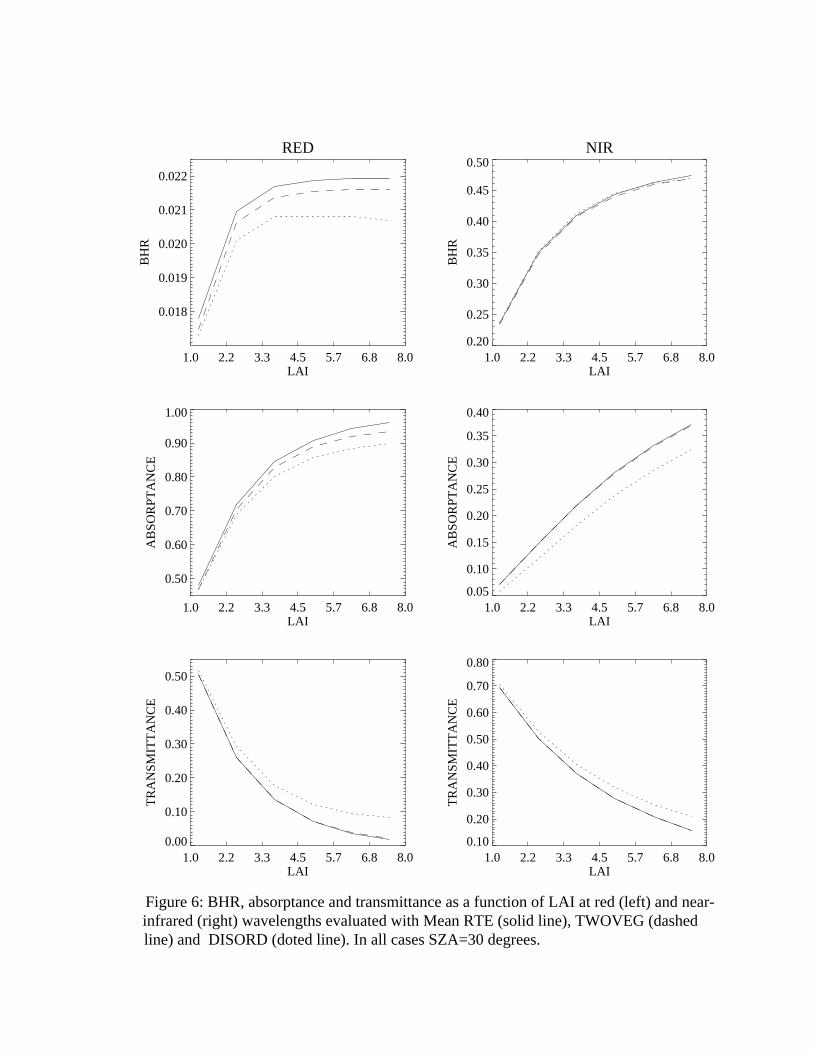
RED

1.0 2.2 3.3 4.5 5.7 6.8 8.0LAI

0.018

0.019

0.020

0.021

0.022

BH

RNIR

1.0 2.2 3.3 4.5 5.7 6.8 8.0LAI

0.20

0.25

0.30

0.35

0.40

0.45

0.50

BH

R

1.0 2.2 3.3 4.5 5.7 6.8 8.0LAI

0.50

0.60

0.70

0.80

0.90

1.00

AB

SOR

PTA

NC

E

1.0 2.2 3.3 4.5 5.7 6.8 8.0LAI

0.05

0.10

0.15

0.20

0.25

0.30

0.35

0.40

AB

SOR

PTA

NC

E

1.0 2.2 3.3 4.5 5.7 6.8 8.0LAI

0.00

0.10

0.20

0.30

0.40

0.50

TR

AN

SMIT

TA

NC

E

1.0 2.2 3.3 4.5 5.7 6.8 8.0LAI

0.10

0.20

0.30

0.40

0.50

0.60

0.70

0.80

TR

AN

SMIT

TA

NC

E

Figure 6: BHR, absorptance and transmittance as a function of LAI at red (left) and near- infrared (right) wavelengths evaluated with Mean RTE (solid line), TWOVEG (dashed line) and DISORD (doted line). In all cases SZA=30 degrees.

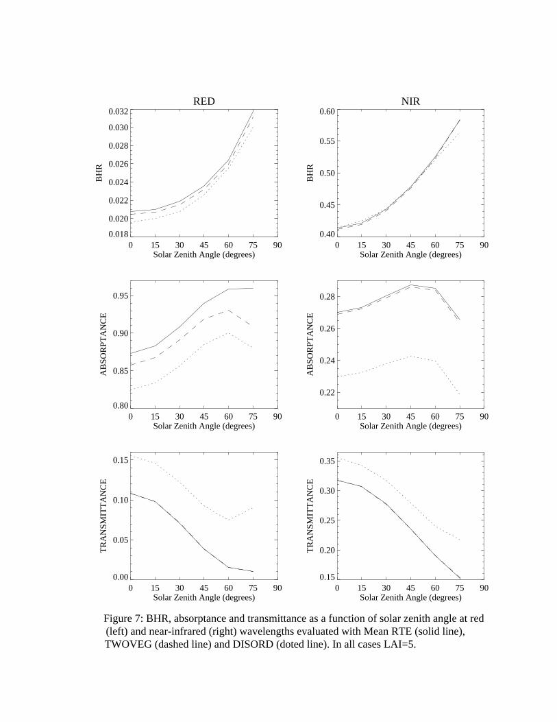
RED

0 15 30 45 60 75 90Solar Zenith Angle (degrees)

0.018

0.020

0.022

0.024

0.026

0.028

0.030

0.032

BH

RNIR

0 15 30 45 60 75 90Solar Zenith Angle (degrees)

0.40

0.45

0.50

0.55

0.60

BH

R

0 15 30 45 60 75 90Solar Zenith Angle (degrees)

0.80

0.85

0.90

0.95

AB

SOR

PTA

NC

E

0 15 30 45 60 75 90Solar Zenith Angle (degrees)

0.22

0.24

0.26

0.28

AB

SOR

PTA

NC

E

0 15 30 45 60 75 90Solar Zenith Angle (degrees)

0.00

0.05

0.10

0.15

TR

AN

SMIT

TA

NC

E

0 15 30 45 60 75 90Solar Zenith Angle (degrees)

0.15

0.20

0.25

0.30

0.35

TR

AN

SMIT

TA

NC

E

Figure 7: BHR, absorptance and transmittance as a function of solar zenith angle at red(left) and near-infrared (right) wavelengths evaluated with Mean RTE (solid line), TWOVEG (dashed line) and DISORD (doted line). In all cases LAI=5.

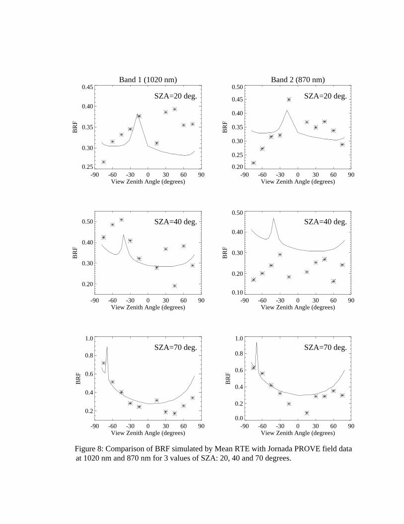
Band 1 (1020 nm)

-90 -60 -30 0 30 60 90View Zenith Angle (degrees)

0.25

0.30

0.35

0.40

0.45

BR

FBand 2 (870 nm)

-90 -60 -30 0 30 60 90View Zenith Angle (degrees)

0.20

0.25

0.30

0.35

0.40

0.45

0.50

BR

F

-90 -60 -30 0 30 60 90View Zenith Angle (degrees)

0.20

0.30

0.40

0.50

BR

F

-90 -60 -30 0 30 60 90View Zenith Angle (degrees)

0.10

0.20

0.30

0.40

0.50

BR

F

-90 -60 -30 0 30 60 90View Zenith Angle (degrees)

0.2

0.4

0.6

0.8

1.0

BR

F

-90 -60 -30 0 30 60 90View Zenith Angle (degrees)

0.0

0.2

0.4

0.6

0.8

1.0

BR

F

SZA=20 deg. SZA=20 deg.

SZA=40 deg. SZA=40 deg.

SZA=70 deg. SZA=70 deg.

Figure 8: Comparison of BRF simulated by Mean RTE with Jornada PROVE field dataat 1020 nm and 870 nm for 3 values of SZA: 20, 40 and 70 degrees.

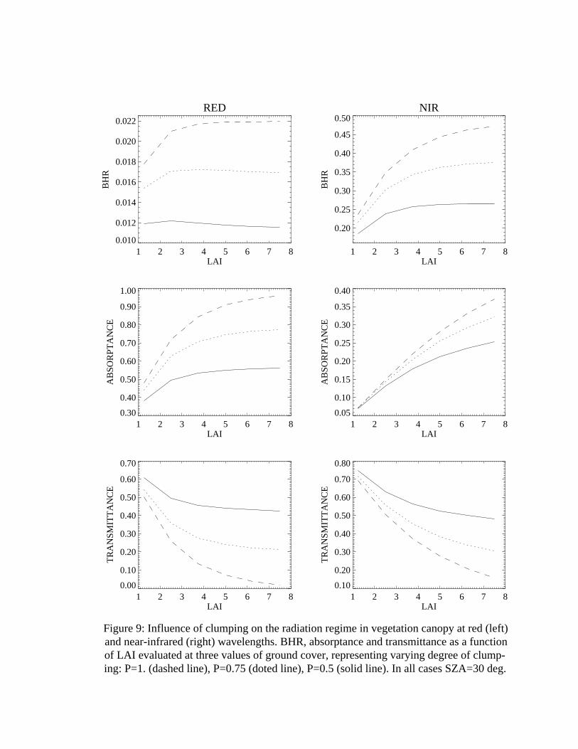
RED

1 2 3 4 5 6 7 8LAI

0.010

0.012

0.014

0.016

0.018

0.020

0.022

BH

RNIR

1 2 3 4 5 6 7 8LAI

0.20

0.25

0.30

0.35

0.40

0.45

0.50

BH

R

1 2 3 4 5 6 7 8LAI

0.30

0.40

0.50

0.60

0.70

0.80

0.90

1.00

AB

SOR

PTA

NC

E

1 2 3 4 5 6 7 8LAI

0.05

0.10

0.15

0.20

0.25

0.30

0.35

0.40

AB

SOR

PTA

NC

E

1 2 3 4 5 6 7 8LAI

0.00

0.10

0.20

0.30

0.40

0.50

0.60

0.70

TR

AN

SMIT

TA

NC

E

1 2 3 4 5 6 7 8LAI

0.10

0.20

0.30

0.40

0.50

0.60

0.70

0.80

TR

AN

SMIT

TA

NC

E

Figure 9: Influence of clumping on the radiation regime in vegetation canopy at red (left)and near-infrared (right) wavelengths. BHR, absorptance and transmittance as a function of LAI evaluated at three values of ground cover, representing varying degree of clump- ing: P=1. (dashed line), P=0.75 (doted line), P=0.5 (solid line). In all cases SZA=30 deg.

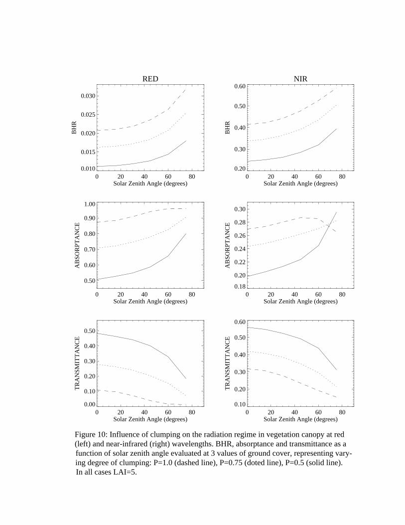
RED

0 20 40 60 80Solar Zenith Angle (degrees)

0.010

0.015

0.020

0.025

0.030

BH

RNIR

0 20 40 60 80Solar Zenith Angle (degrees)

0.20

0.30

0.40

0.50

0.60

BH

R

0 20 40 60 80Solar Zenith Angle (degrees)

0.50

0.60

0.70

0.80

0.90

1.00

AB

SOR

PTA

NC

E

0 20 40 60 80Solar Zenith Angle (degrees)

0.18

0.20

0.22

0.24

0.26

0.28

0.30

AB

SOR

PTA

NC

E

0 20 40 60 80Solar Zenith Angle (degrees)

0.00

0.10

0.20

0.30

0.40

0.50

TR

AN

SMIT

TA

NC

E

0 20 40 60 80Solar Zenith Angle (degrees)

0.10

0.20

0.30

0.40

0.50

0.60

TR

AN

SMIT

TA

NC

E

Figure 10: Influence of clumping on the radiation regime in vegetation canopy at red (left) and near-infrared (right) wavelengths. BHR, absorptance and transmittance as a function of solar zenith angle evaluated at 3 values of ground cover, representing vary- ing degree of clumping: P=1.0 (dashed line), P=0.75 (doted line), P=0.5 (solid line). In all cases LAI=5.

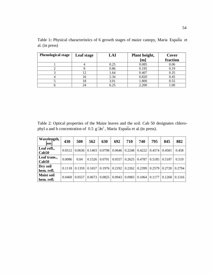
54

Table 1: Physical characteristics of 6 growth stages of maize canopy, Maria an~Espa etal. (in press)

Phenological stage Leaf stage LAI Plant height,[m]

Coverfraction

1 4 0.25 0.085 0.062 8 0.86 0.195 0.193 12 1.64 0.407 0.354 16 2.34 0.820 0.455 18 3.01 1.800 0.556 24 6.25 2.200 1.00

Table 2: Optical properties of the Maize leaves and the soil. Cab 50 designates chloro-phyl a and b concentration of 0.5 2mg ⋅ , Maria ).pressin(.aletan~Espa

Wavelength,[ ]nm 430 500 562 630 692 710 740 795 845 882

Leaf refl.,Cab50

0.0512 0.0636 0.1403 0.0798 0.0646 0.2248 0.4222 0.4574 0.4581 0.458

Leaf trans.,Cab50

0.0086 0.04 0.1526 0.0791 0.0557 0.2625 0.4787 0.5185 0.5187 0.519

Dry soilhem. refl.

0.1118 0.1359 0.1657 0.1976 0.2192 0.2262 0.2399 0.2579 0.2720 0.2794

Moist soilhem. refl.

0.0469 0.0557 0.0673 0.0825 0.0943 0.0983 0.1064 0.1177 0.1268 0.1316