Stochastic Modeling and Simulation of

Viral Evolution

Luiza Guimaraes1 Diogo Castro1 Bruno Gorzoni1

Luiz Mario Ramos Janini2 Fernando Antoneli3,∗

October 19, 2018

Abstract

RNA viruses comprise vast populations of closely related, but highlygenetically diverse, entities known as quasispecies. Understanding themechanisms by which this extreme diversity is generated and maintainedis fundamental when approaching viral persistence and pathobiology ininfected hosts. In this paper we access quasispecies theory through aphenotypic model, to better understand the roles of mechanisms resultingin viral diversity, persistence and extinction. We accomplished this by acombination of computational simulations and the application of analytictechniques based on the theory of multitype branching processes. In orderto perform the simulations we have implemented the phenotypic modelinto a computational platform capable of running simulations and present-ing the results in a graphical format in real time. Among other things, weshow that the establishment virus populations may display four distinctregimes from its introduction to new hosts until achieving equilibriumor undergoing extinction. Also, we were able to simulate different fit-ness distributions representing distinct environments within a host whichcould either be favorable or hostile to the viral success. We addressed themost used mechanisms for explaining the extinction of RNA virus popu-lations called lethal mutagenesis and mutational meltdown. We were ableto demonstrate a correspondence between these two mechanisms imply-ing the existence of a unifying principle leading to the extinction of RNAviruses.

keywords: Viral evolution, Quasispecies theory, Multitype branching process,Lethal mutagenesis, Mutational meltdown

1Programa de Pos-Graduacao em Infectologia, Universidade Federal de Sao Paulo, SaoPaulo, SP, Brazil.

2Departamentos de Microbiologia, Imunologia, Parasitologia and Medicina, UniversidadeFederal de Sao Paulo, Sao Paulo, SP, Brazil.

3Departamento de Informatica em Saude and Laboratorio de Biocomplexidade e GenomicaEvolutiva, Universidade Federal de Sao Paulo, Sao Paulo, SP, Brazil.

∗Corresponding author. E-mail: fernando.antoneli@unifesp.br

1

arX

iv:1

706.

0464

0v2

[q-

bio.

PE]

10

Nov

201

7

1 Introduction

Viruses with RNA genomes, the most abundant group of human pathogens [26],exhibit high mutational rates, fast replicative kinetics, large population sizes,and high genetic diversity. Current evidences also indicate that RNA viruspopulations consist of a wide and interrelated distribution of variants, which candisplay complex evolutionary dynamics. The complex evolutionary propertiesof RNA virus populations features the modulation of viral phenotypic traits, theinterplay between host and viral factors, and other emergent properties [28, 27].During viral infections, these features allow viral populations to escape from hostpressures represented by the actions from the immune system, from vaccines andto develop resistance antiviral drugs. Taken together these features representthe major obstacle for the success and implementation of effective therapeuticintervention strategies.

In order o describe the evolution of RNA viruses and its relationship withtheir hosts and antiviral therapies, theoretical models of virus evolution havebeen developed. These models employ mathematical and computational toolsas methodological instruments allowing one to address evolutionary questionsfrom a different perspective than the commonly seen use of modern experimentaltechnologies. This kind of approach allows the implementation of low-cost re-search projects addressing evolutionary questions that are usually investigatedby experimental methods. In a deeper level, they provide a systematic per-spective of the biological phenomenon, when viewed as proof-of-concept mod-els [90]. Verbal or pictorial models have long been used in evolutionary biologyto formulate abstract hypotheses about processes and mechanisms that operateamong diverse species and across vast time scales. Used in many fields, proof-of-concept-models test the validity of verbal or pictorial models by laying outthe underlying assumptions in a mathematical framework.

Eigen and Schuster [36, 38] proposed and analyzed a deterministic model forthe evolution of polynucleotides in a dialysis reactor based on a system of ordi-nary, differential equations called quasispecies model. Subsequently, Demetriuset al. [23] proposed a stochastic quasispecies model in order to overcome somedrawbacks of the deterministic quasispecies model of Eigen and Schuster [38].The approach of Demetrius et al. [23] employed very powerful methods basedon the theory of stochastic branching processes. This theory, originally devel-oped to deal with the extinction of family names (Watson and Galton [96]), hasbeen applied since the forties to a great variety of physical and biological prob-lems [48, 6, 57]. On the experimental side, an early study of the RNA phage Qβreporting that sequence variation in a population was high but approximatelystable over time around a consensus sequence, gave the initial stimulus to con-sider the notion of quasispecies in the broader context of RNA viruses [29].Since then, quasispecies theory has been recognized as a subset of theoreticalpopulation genetics – being mathematically equivalent to the theory of multi-loci mutation-selection balance in the limit of infinite populations [97, 92, 21, 15]– and, due to is a capability to deal with high mutation rates, has been widelyapplied to model the evolution of viruses with RNA genomes [37].

2

Inspired by the stochastic quasispecies model of Demetrius et al. [23] andbased on branching process techniques, Antoneli et al. [4, 5] proposed a mathe-matical framework aimed at understanding the basic mechanisms and phenom-ena of the evolution of highly-mutating viral populations replicating in a singlehost organism, called phenotypic (quasispecies) model. It is denominated “phe-notypic” due to the fact that it only comprises probabilities associated to theoccurrence of deleterious, beneficial and neutral effects that operate directly onthe replicative capability of viral particles, without any explicit reference to theirgenotypes. In [22] Dalmau introduced another generalization of the stochasticquasispecies model also based on multitype branching processes but retainingthe genotypic character of Demetrius et al. [23].

The phenotypic model [4, 5] is defined through a probability generatingfunction which formally determines the transition structure of the process. Thematrix of first moments of the branching process, or simply the mean matrix,defines a deterministic linear system which describes the time evolution of con-ditional expectations, a “mean field model” for the actual stochastic processwhich is equivalent to the Eigen’s selection equation [23]. The deterministicmean field model has been studied by several researches, but without the con-nection to a stochastic branching process, see for instance [7, 68, 19] In [4] theauthors carry out a thorough analysis of mean matrix, assuming that beneficialeffects are absent and were able to show that the phenotypic model is “exactlysolvable”, in the sense that the spectral problem for the mean matrix has anexplicit solution. In [5] the authors employ spectral perturbation theory in orderto treat the general case of small beneficial effects. This approach has provideda complete description of the average behavior of the model.

In the present paper, we further address the biological implications of model-ing RNA virus populations in terms of the phenotypic model. We achieved thisgoal by a combination of computational simulations and the basic analytic tech-niques of the theory of multitype branching processes. In order to perform thesimulations we have implemented the phenotypic model into a computationalplatform capable of running the simulation and presenting the results in graph-ical format in real time. As we shall see, the phenotypic model is fully specifiedby three fundamental parameters: the probabilities of occurrence of deleteriousand beneficial effects d and b – the probability of occurrence of neutral effects isfixed by the complementarity relation c = 1−d− b – and the maximum replica-tive capability R. By an exhaustive analysis of this “parameter space” we wereable portray a fairly detailed outline of all possible behaviors of the model. Amultitype branching process may be classified into three distinct regimes:

Stationary regime. In the phenotypic model it corresponds to the asymp-totic behavior of a super-critical branching process. At the end of a transientphase the viral population exhibits a steady viral load and stable relative fre-quencies of almost all variants in the population. At this point the viral popu-lation has recovered its phenotypic diversity and becomes better adapted to thenew host environment. It represents an advanced stage of the infection, called

3

chronic infection phase. We obtain explicit expressions for the relative frequen-cies of the replicative classes and other quantities derived from them such asthe average reproduction rate of the viral population, the phenotypic diversityand the phenotypic entropy.

Threshold of extinction. In the phenotypic model, it corresponds to a crit-ical branching process. The threshold of extinction takes place when the dele-terious rate is sufficiently high that it prevents the viral population of reachingthe stationary regime but not high enough to induce the extinction of the pop-ulation in the short run. We show that this regime is completely determinedby a particular value of the deleterious probability, called critical deleteriousprobability. We provide an explicit expression for this quantity. We also findan asymptotic expression for the maximum beneficial probability at which theextinction threshold disappears and the population no longer can extinguished.

Extinction by Lethal Mutagenesis. In the phenotypic model, it corre-sponds to a sub-critical branching process. It is the process of extinction of theviral population due to the increment of the deleterious rate and is characterizedby a distinct signature observed in the time series of the average reproductionrate, during a simulation: an explosive growth in the variation of the averagereproduction rate as it approaches the extinction time. We given an expressionfor the expected time to extinction in terms of the parameters d, R and thecritical deleterious probability. We also show that when then deleterious prob-ability approaches its critical value, and the branching process approaches itsextinction threshold, the model displays a scaling law that resembles a “phasetransition” with critical exponent 1.

In addition to this classification into distinct regimes, we give a characteri-zation of the initial time evolution of the the model and discuss the role of thefitness distributions on the variance of the branching process.

Transient phase and recovery time. The initial phase of the time evo-lution of a branching process, which corresponds to the beginning of the viralinfection occurring after a transmission bottleneck when a very limited num-ber of particles are transmitted. It comprises the acute infection phase and ischaracterized by an initial exponential growth of the population, resulting in aviremia peak, followed by a slower viral load decrease towards the stabilizationof the population size (also referred as viral set point in clinical settings). Theexpected time (represented in the model by the number of viral generations) forthe relaxation towards an equilibrium is called recovery time. We put forward anatural way to define the recovery time in terms of a characteristic time derivedfrom the decay of the mean auto-correlation function of the branching processand we deduce an expression for the characteristic time in terms of d, b and R.

Fitness distributions. These are location-scale families of discrete distribu-tions that control progeny sizes at each replication cycle. They can be seen as

4

representing distinct “compartments” in the host which can be more favorableor pose restrictions to the viral replication process. For instance, some distribu-tions have a positive influence on the replication, by enhancing the replicationof particles in the higher replicative classes, while other distributions have anopposite effect. Examples of favorable compartments would be sites associatedwith immune privilege, or with lower concentration of antiviral drugs, or al-lowing for cell to cell virus transmission. Unfavorable compartments are siteswith high antiviral drug penetration, small number of target cells, or accessedby elements of host responses as antibodies, citotoxic cells and others. In thissense, we may think of fitness distributions as an environmental componentduring viral evolution. We showed that the impact of the fitness distributionson the branching process is subtle and can not be detected by quantities thatdepend only on the first moments of the process. Nevertheless, a new quantity,called populational variance, is capable to detect the influence of different fitnessdistributions.

Finally, we propose a unifying principle underlying two mechanisms of ex-tinction of a virus population.

Mechanisms of extinction. A virus population can be become extinct oreradicated from the host by the fulfillment of a condition involving only theprobability of occurrence of deleterious effects d and the maximum replicativecapability R. Even further, in the absence of beneficial or compensatory effects,the fate of the population becomes entirely settled whether the product R(1−d)is greater or lesser than 1. Based on this observation we show that there is acorrespondence between two well known distinct mechanisms of extinction:

(a) Lethal Mutagenesis. The process of extinction of the viral population dueto the increment of the deleterious rate [9, 10].

(b) Mutational Meltdown. The process of extinction of the viral populationthrough the step-wise loss of the fittest replicative classes due to randomdrift associated to the finite population size effect [66, 65].

Here there is a new component of the phenotypic model that comes intoplay: the carrying capacity K. Initially, the carrying capacity is introducedas a convenient device for the computational implementation of the phenotypicmodel, by providing an upper bound for the population size. Nevertheless, itcan be seen as genuine component of the phenotypic model if we regard themodel as a self-regulated branching process, instead of a “pure” branching pro-cess. Within this extended framework, we show that a phenotypic analogue ofthe mutational meltdown criteria for extinction comes out from the same rela-tion that determines the fate of the population during the lethal mutagenesis.Furthermore, we observe that the process of extinction in this case has a verydistinct signature, when compared with the lethal mutagenesis, resembling a“lingering ratchet”, which “clicks” each time a replicative class is purged. Thecorrespondence between the two mechanisms results from the following obser-vations. Lethal mutagenesis occurs by the loss of the fittest replicative classes

5

when the deleterious mutational rate is sufficiently high. This will occur evenwhen the carrying capacity reaches infinite values. Mutational meltdown alsooccurs when the fittest replicative classes are lost by random drift due to the fi-nite size effect induced by the carrying capacity. In the mutational meltdown thedeleterious rate may not be negligible but is much lower than in lethal mutagen-esis. Therefore, losing the best adaptative classes due to increasing mutagenesisor to small population size effects in a phenotypic model framework are indeed“two sides of the same coin” [70].

Structure of the paper. The paper is structured as follows. In section 2 weintroduce the phenotypic model starting with the biological motivation followedby the mathematical definition. In section 3 we recall the main theoreticalresults of [4, 5] and introduce the computational platform for the simulation ofthe phenotypic model. In section 4 we explore the consequences of the modelusing the theoretical results explained in the previous section coupled with theanalysis of simulations. These three sections are somewhat independent andcan be skipped or read in reverse order, by readers familiarized with [4, 5]. Thepaper ends with a conclusion section. There are two appendices providing sometheoretical details used in the paper.

2 Phenotypic Model for Viral Evolution

In this section we introduce the phenotypic model for viral evolution first bylaying out the underlying biological foundations on which it is based on andthen presenting its natural mathematical description as a multitype branchingprocess.

2.1 Biological Foundations

It is usual in population genetics to consider that the whole set of individu-als composing a population reproduce at the same time in such a way thatthe evolution of the population is described as a discrete succession of gen-erations [63, 16]. The time between any two successive generations is calledgeneration time. In the context of viral populations the generation time willdepend on the cellular status and extracellular environment. Because virusesare obligate intracellular parasites, production of progeny particles may vary intime and in exuberance depending on the metabolic status of an infected cellat the time of virus production. As a result, the meaningful concept of virusgeneration time is a distribution of generation times with a well-defined meanvalue. Thus, the generation time can represent, in the study of viral evolution,the average duration of time between two identical and successive replicationcycles of a viral population. Under these conditions, one may consider that noparticle can be part of two successive generations, that is, the generations arediscrete and non-overlapping. Therefore, the dynamics of the population pro-ceeds in replication cycles, in which each viral particle of a generation produces,

6

according to its replicative capability, the viral particles of the next generation.In natural systems, the replicative capability of a viral particle is a phe-

notypic trait, and is product of a complex interaction between the expressedgenotypic composition of the particle and the intracellular and extracellularenvironments in which it is inserted. Consequently the same replicative capa-bility can be expressed by different viral genotypes, a phenomenon known asrobustness [94, 61], which has been identified to occur in sets of diverse viralsequences bearing mutations that are selectively neutral and connected throughneutral networks [94, 46]. On the other hand, viruses with the same genomecomposition may show different replication capabilities if they infect cells atdifferent cellular status. The variation of cellular status over time may influencethe number of progeny particles that are produced by different cells yieldingbroad distributions of progeny sizes [99], called fitness distributions. For thisreason, it makes sense to consider subsets of particles that have the same “po-tential replicative capability”, as comprising replicative classes within the viralpopulation and representing viral genotypes that express the same fitness distri-bution. Therefore, each replicative class may be characterized be a well definedmean replicative capability that is a non-negative integer ranging from zero toa fixed maximum value R, called maximum replicative capability. The maxi-mum replicative capability of a population reflects the intrinsic limitations ofthe virus replication machinery and the host organism environment (such asspace restriction, availability and finiteness of resources, etc.). Formally, themaximum replicative capability is defined as the maximum number of progenya viral particle can produce from one infected cell. This particles will go on toestablish infections in other cells.

In general, the measurement of R is highly non-trivial. One may write R asthe product of two quantities, S and B (R = SB), where S is the success rate,corresponding to the success of progeny particles in establishing infections innew cells, and B is the burst size, corresponding to the number of total viableviral offspring released from a cell infected by a virus particle [9]. Typically, theburst size B is a number much larger than 1 while the success rate S is alwaysstrictly smaller than 1 thus, R may be much less than the number of offspring Bper infected cell, because the success rate may be very low. Indeed, histologicalobservations on plants inoculated with tobacco mosaic virus suggest that R maybe as low as 3 to 6 particles per cell [67] and, on the other hand, the in vivoburst size of SIV was estimated to be of the order of 104 virions per cell [17],which together suggest that the success rate might be as low as 10−4.

The evolution of RNA viral populations is a physical process strongly in-fluenced by randomness, which is ultimately represented by the incorporationof random mutations. The effects of new mutations on the fitness are oftenclassified as being deleterious, neutral or beneficial, but there is, in reality, acontinuous distribution of fitness effects, stretching from those that are lethalto mutations that are highly beneficial [39]. Mutations produce the geneticvariability of viral populations over which selective pressures act on. The highmutation rates of RNA viruses, ranging from 10−4 to 10−6 nucleotide substi-tutions per site per genome replication [35, 89], are primarily associated to the

7

intrinsic low fidelity of their replication machinery. Furthermore, the chancesof mutations to have an impact on fitness are increased in RNA viruses due tothe relatively small size of their genome, the presence of overlapping open read-ing frames and the fact that mostly all nucleotides have structural and codinginformation.

When rates of spontaneous mutation are expressed per genome replication,different broad groups of organisms display characteristic values [33, 34]: ofthe order of 0.001 for DNA-based microbes (including both viral and cellularorganisms); of the order of 0.01 for higher eukaryotes; from the order of 0.01 tothe order of 0.1 for retroviruses and from the order of 0.1 to the order of 1 forRNA viruses exclusive of retroviruses [49, 91, 3, 32]. This wide range of mutationrates of RNA viruses suggests that it is inappropriate to gather RNA virusestogether into a single group that is subject to different evolutionary rules thanorganisms with DNA genomes. Nevertheless, accurate quantification of thoserates is difficult, most notably due to their dependence on tiny mutation reportersequences that may not well represent the whole genome and the uncertainty dueto the combination of mutation frequencies and population history to calculatemutation rates [31]. In addition, independent estimates may give the sameorder of magnitude but have fairly different significant digits. For instance,three estimates of the HIV-1 mutation rate [69, 79, 1] range from 3.5 × 10−5,8.5×10−5, 1.4×10−5 nucleotide substitutions per site per genome replication.

In a purely phenotypic approach to evolution there is no direct reference torandom mutations, since there is no phenotype-to-genotype map. Therefore, theaction of mutations as a driving force of evolution is indirectly represented bychanges in the distribution of fitness effects [39]. Moreover, from the phenotypicpoint of view an effect associated to a neutral mutation is undistinguishable fromthe non occurrence of a mutation, since both result in no (or negligible) change inthe relative fitness. By including the non-occurrence of mutations in the neutraleffects one may consider that a fitness effect occurs with probability 1 to everyprogeny particle produced during a replication cycle. Therefore, the combinedaction of genetic and non-genetic causes produces three types of fitness effectsapplicable to every single replication event:

Deleterious effects. These effects cause changes that eventually occur during theproduction of the viral progeny that may decrease the replicative capability ofthe progeny. In RNA viruses, the deleterious effects of genetic mutations resultsin a progeny displaying a lower replication capability because these mutationsaffects sites that code for amino acids important for the functionality of viralproteins or disturb the formation of three-dimensional structures of the viralRNA. Indirectly, in a strict phenotypic model we should consider as deleteri-ous effects pressures exerted by humoral and cellular immune responses as wellas antiviral treatments, since they altogether will reduce the virus replicativecapability.

Beneficial effects. These effects cause changes that eventually occur during theproduction of the viral progeny that may increase the replicative capability ofthe progeny. This increase can be caused, for example, by point or multiple

8

mutations that allow the particle to improve its replication efficiency, escapefrom the responses of the immune system, escape from the antiviral drug activityor by environmental changes favorable for viral adaptation. The probability ofoccurrence of a beneficial effect is less than or equal to the probability occurrenceof a deleterious or neutral effects. The relative frequencies between beneficial,deleterious and neutral mutations appearing in a replicating population havebeen already measured by prior studies [72, 50, 53, 80, 88, 14, 39, 81, 85]. Takingtheir results together, it is reasonable to conclude that beneficial mutations couldbe as low as 1000 less frequent than either neutral or deleterious mutations. Asa result, the viral population would be submitted to a large number of successivedeleterious and neutral changes and a comparatively small number of beneficialchanges.

Neutral effects. These are effects that cause changes that eventually occur dur-ing the production of the viral progeny that do not increase or decrease thereplicative capability of the progeny. Changes that eventually occur during thereplication can be neutral when, for example, they do not replace the aminoacids coded by the viral genome (synonymous mutations) and they do not re-place genomic sequence associated with structural RNA function. Or it mightrepresent situations in which the cellular and extracellular environments havenot undergone substantial changes that could affect the general fitness of viralparticles.

Consequently, a phenotypic model concentrates all the above mentioned fit-ness effects in probabilities the act independently on every single particle in thepopulation. As a result, when discussing the simulations we mention that thereplicative capability of a particle has changed, we are taking into account allthe above mentioned effects.

In a model where fitness is the only feature that can be “observed” the meannumber of successful offspring per individual particle, called average reproduc-tion rate and denoted by µ, is the most relevant quantity to be considered. Inthe context of virus infections host, it may be seen as a measure of whether avirus can establish a new infection or not. It is the mean number of particles in-fecting cells that will produce particles able to infect other cells when there is nolimitations in the number of target cells. In a mutation-free population it is ex-pected that µ is equal to the maximum replicative capability R. However, in thecase of RNA viruses that replicate under high mutational rates the mutationalspectra and its effects should be taken into account. If only deleterious andneutral effects are present then µ is expected to be proportional to R, namelyµ = R w, where w represents the relative fitness level and is a function of theprobabilities of occurrence of deleterious and/or neutral effects. The product ofthe relative fitness level w by the maximum replicative capability R furnishes ameasure of populational fitness, i.e., mean number of progeny per particle. Invivo estimates of µ have been accomplished in some cases, for instance, in [84]the value of mean reproduction rate during acute HIV-1 infection was estimatedto be 8.0 with an interquartile range of 4.9 to 11.

The importance of the mean reproduction rate µ stems from the fact that it

9

is the key quantity associated to the the mechanism of lethal mutagenesis, putforward by Bull et al. [9] to explain the extinction process of viral populations.If µ is less than 1, on average an infected cell will produce a progeny able toinfect less than 1 susceptible cell, and the infection will die out; if µ is greaterthan 1, on average an infected cell will produce a progeny able to infect morethan 1 susceptible cell, and generally the infection will spread.

It turns out, as shown in [4, 5], that phenotypic model affords a natural in-terpretation of the relative fitness level µ in the context of branching processes,which allowed us to obtain a simple expression for µ that is formally equiva-lent to the extinction criterion of the theory of lethal mutagenesis for viruses ofBull et al. [9]. In the absence of beneficial effects, it follows that w is exactlythe probability of occurrence of a neutral effect and, in general, this holds ap-proximately, up to first order in perturbation with respect to the probability ofoccurrence a beneficial effect (see equation (7)). The branching process formu-lation allows for an interpretation of µ as the average exponential growth rate ofthe population, called the malthusian parameter [57]. Within this framework,a new interpretation of the lethal mutagenesis criterion [9] emerges naturallyas the sub-criticality of a branching process: it is a sufficient condition for thepopulation to become extinct in finite time.

The lethal mutagenesis extinction threshold is, to some extent, related tothe error catastrophe derived by Eigen [36] for the deterministic model. In fact,Demetrius et al. [23] already observed that the extinction criterion provided bythe classification of a branching process, in the context of their stochastic quasis-pecies model, formally resembles the deterministic error catastrophe. But, whilethe deterministic error catastrophe refers to the condition to replicate with afidelity above the error threshold, the stochastic extinction criterion refers tothe probability of extinction. Consequently, the demand to function above theextinction threshold is always a stronger condition than the corresponding re-quirement of the deterministic error threshold. However, the error catastrophephenomenon as such, makes no statements about population extinction. Eventhough the concept of error catastrophe has been widely cited as the under-lying theory in several studies reporting the occurrence of extinction of viruspopulations [82, 18, 3], it is the notion of lethal mutagenesis (and the corre-sponding extinction criterion) that is relevant to the occurrence of extinction inviral populations [97, 92].

Inspired by ideas from population genetics, more specifically the “Muller’sRatchet”, Lynch and Gabriel [66] a mechanism for the process of extinction ofasexual populations, in particular, RNA virus populations, called mutationalmeltdown. The “Muller’s Ratchet” [75, 41] describes the step-wise loss of thefittest class of individuals in a population and the associated reduction in ab-solute fitness due to the accumulation of deleterious effects. The mechanismof mutational meltdown works only for finite populations and is based on theaction of random drift. The mutational meltdown theory predicts the eventualextinction of the population if there is no compensatory or beneficial effects. Inthe absence of compensatory mechanisms the process leads the population to the“meltdown” phase (Lynch et al. [65]): the population will face extinction when

10

the mean viability w (the probability of occurrence of a neutral effect per mu-tation raised to mean number of mutations carried by an individual) decreasesbelow the reciprocal of the absolute growth rate R (the maximum number ofoffspring an individual can produce).

Despite the different backgrounds from which the lethal mutagenesis and themutational meltdown were developed, there is a considerable amount of paral-lelism between them. There seems to be a strait correspondence between thenotions of “relative fitness level” and “maximum replicative capability” derivedfrom the lethal mutagenesis theory and “mean viability” and “absolute growthrate” derived from the mutational meltdown theory. Furthermore, the apparentdisparity between the two approaches – at least in their simplest forms, “Er-ror Threshold” versus “Muller’s Ratchet” – has been addressed by Wagner andKrall [95], who observed that the discrepancy is due to different assumptionsregarding the possible fitness values the mutants are allowed to assume.

2.2 Mathematical Definition

Based on the general aspects of the phenomenon of viral replication describedbefore it is compelling to model it in terms of a branching process. In thisperspective we shall consider a discrete-time multitype Galton-Watson branchingprocess for the evolution of an initial population with types or classes which areindexed by a non-negative integer r ranging from 0 to the average maximumreplicative capability R. The branching process is described by a sequence ofvector-valued random variables Zn = (Z0

n, . . . , ZRn ), (n = 0, 1, . . .), where Zrn

is the number of particles of replicative class r in the n-th generation. Theinitial population Z0 is represented by a vector of non-negative integers (alsocalled multi-index ) which is non-zero and non-random. The time evolution ofthe population is determined by a vector-valued discrete probability distributionζ(i) =

(ζr(i)

), defined on the set of multi-indices i = (i0, . . . , iR), called the

offspring distribution of the process, which is usually encoded as the coefficientsof a vector-valued multivariate power series f(z) =

(fr(z)

)called probability

generating function (PGF):

fr(z0, z1, . . . , zR) =∑ir

ζr(i0, . . . , iR) zi

0

0 . . . ziR

R , r = 0, . . . , R .

At each replicative cycle, each parental particle in the replicative class r pro-duces a random number of progeny particles that is independently drawn accord-ing to the corresponding fitness distribution belonging to a location-scale familyof discrete probability distributions tr (r = 0, . . . , R) assuming non-negativeinteger values and normalized so that their expectation value is

∑k k tr(k) = r

and t0(k) = δk0. Therefore, each particle in the viral population is charac-terized by the mean value of its fitness distribution, called mean replicativecapability. Viral particles with replicative capability equal to zero (0) do notgenerate progeny; viral particles with replicative capability one (1) generate oneparticle on average; viral particles with replicative capability two (2) generate

11

two particles on average, and so on. Typical examples of location-scale familiesof discrete probability distributions that can be used as fitness distributions are:

(a) the family of Deterministic (Delta) distributions: tr(k) = δkr.

(b) the family of Poisson distributions: tr(k) = e−r rk

k! .

Note that in the first example, the replicative capability is completely concen-trated on the mean value r – that is, the particles have deterministic fitness.On the other hand, in the second example the fitness is truly stochastic.

During the replication, each progeny particle always undergoes one of thefollowing effects:

deleterious effect: the mean replication capability of the respective progenyparticle decreases by one. Note that when the particle has capability ofreplication equal to 0 it will not produce any progeny at all.

beneficial effect: the replication capability of the respective progeny particleincreases by one. If the mean replication capability of the parental particleis already the maximum allowed then the mean replication capability ofthe respective progeny particles will be the same as the replicative capa-bility of the parental particle.

neutral effect: the mean replication capability of the respective progeny par-ticle remains the same as the mean replication capability of the parentalparticle.

To define which effect will occur during a replication event, probabilities d, band c are associated, respectively, to the occurrence of deleterious, beneficialand neutral effects. The only constraints these numbers should satisfy are 0 6d, b, c 6 1 and b+c+d = 1. In the case of in vitro experiments with homogeneouscell populations the probabilities c, d and b essentially refer to the occurrenceof mutations.

The determination the offspring probability distribution ζ of the phenotypicmodel is more transparent if one assumes first that b = 0 and tr(k) = δkr. Inthis case, we have that d+ c = 1 and the number of progeny particles producedby any particle of replicative class r is exactly r. Then ζr(i) is non-zero onlywhen the multi-index i is of the form i = (0, . . . , ir−1, ir, . . . , 0), since a particlewith replicative capability r can only produce progeny particles of the replicationcapability r or r−1. Moreover, the entries ir−1 and ir satisfy ir−1+ir = r. Thuswe just need to compute the probabilities ζr for the multi-indices of the form(0, . . . , r − k, k, . . . , 0). Suppose that a viral particle with replicative capabilityr (0 6 r 6 R) replicates itself producing r new virus particles v1, . . . , vr. Foreach new particle vj , there are two possible outcomes regarding the type ofchange that may occur: neutral or deleterious, with probabilities c = 1 − dand d, respectively. Representing the result of the j-th replication event by avariable Xj , which can assume two values: 0 if the effect is deleterious (failure)and 1 if the effect is neutral (success), the probability distribution of Xj is that

12

of a Bernoulli trial with probability of occurrence of a neutral effect c = 1− d(success), that is,

P(Xj = k) = (1− d)k d1−k (k = 0, 1) .

The total number of neutral effects that occur when the original virus particlereproduces is a random variable Sr = X1 + · · · + Xr given by the sum of allvariables Xj , since each copy is produced independently of the others. That is,Sr counts the total number of neutral effects (successes) that occurred in theproduction of r virus particles v1, . . . , vr. It also represents the total number ofparticles that will have the same replication capability r of the original particlev. It is well known [40] that a sum of r independent and identically distributedBernoulli random variables with probability c = 1−d of success has a probabilitydistribution given by the binomial distribution:

P(Sr = k) = binom(k; r, 1− d) =

(r

k

)(1− d)k dr−k .

Since this is the probability that a class r virus particle produces k progenyparticles with the same replicative capability as itself, one has

ζr(0, . . . , r − k, k, . . . , 0) = binom(k; r, 1− d) .

From the previous calculation one obtains that the PGF of the phenotypic modelwith b = 0 and tr(k) = δkr is

f0(z0, z1, . . . , zR) = 1

f1(z0, z1, . . . , zR) = dz0 + cz1

f2(z0, z1, . . . , zR) = (dz1 + cz2)2

...

fR(z0, z1, . . . , zR) = (dzR−1 + czR)R

(1)

Note that the functions fr(z0, z1, . . . , zR) are polynomials whose coefficients areexactly the probabilities of the binomial distribution binom(k; r, 1− d). Now itis easy to obtain the PGF in the case with general beneficial effects and witha general family of fitness distribution (which reduces to the previous PGF forthe particular case discussed before).

f0(z0, z1, . . . , zR) = 1

f1(z0, z1, . . . , zR) =

∞∑k=0

t1(k) (dz0 + cz1 + bz2)k

f2(z0, z1, . . . , zR) =

∞∑k=0

t2(k) (dz1 + cz2 + bz3)k

...

fR(z0, z1, . . . , zR) =

∞∑k=0

tR(k) (dzR−1 + (c+ b)zR)k

(2)

13

Note that in the last equation the beneficial effect acts like the neutral effect.This is a kind of “consistency condition” ensuring that the populational replica-tive capability is, on average, upper bounded by R. Even though it is possiblethat a parental particle in the replicative classes R eventually has more thanR progeny particles when tr is not deterministic, the average progeny size isalways R.

Finally, it is easy to see that the PGF of the two-dimensional case of thephenotypic model with b = 0 and z0 = 1 (and ignoring f0) reduces to

f(z) =

∞∑k=0

t(k) ((1− c) + cz)k =

∞∑k=0

t(k) (1− c(1− z))k . (3)

This is formally identical to the PFG of the single-type model proposed by [23, p.255, eq. (49)] for the evolution of polynucleotides. In their formulation, c = pν isthe probability that a given copy of a polynucleotide is exact, where the polymerhas chain length of ν nucleotides and p is the probability of copying a singlenucleotide correctly. The replication distribution t(k) provides the number ofcopies a polynucleotide yields before it is degraded by hydrolysis.

3 Analysis and Simulation of the PhenotypicModel

In this section we recall some basic results on the mathematical properties ofthe phenotypic model, obtained [4, 5] and introduce a computational platformfor its simulation.

3.1 Mathematical Basis of the Phenotypic Model

A remarkable property of the phenotypic model that was fully explored in An-toneli et al. [4, 5] is the fact that when b = 0 the phenotypic model is “exactlysolvable” in a very specific sense. One of the main quantities associated to amultitype branching process is its “asymptotic growth rate”, which is measuredby the malthusian parameter µ. It may be defined as the limit when number ofparticles goes to infinity of the “average reproduction rate”, namely, the averagenumber of of offspring per particles per generation. From the general theory ofbranching processes it follows that µ can be obtained as the largest eigenvalueof the matrix of first moments of the process.

The mean matrix or the matrix of first moments M = {Mij} of a multi-type branching process describes how the average number of particles in eachreplicative class evolves in time and is defined by Mij = E(Zi1|Z

j0 = 1) where

Zj0 = 1 is the abbreviation of Z0 = (0, . . . , 1, . . . , 1). In terms of the probabilitygenerating function f = (f0, . . . , fR) it is given by

Mij =∂fj∂zi

(s)

∣∣∣∣s=1

(4)

14

where 1 = (1, 1, . . . , 1).It is straightforward form the generating function (2), using formula (4),

that the matrix of the phenotypic model is given by

M =

0 d 0 0 0 . . . 00 c 2d 0 0 . . . 00 b 2c 3d 0 . . . 00 0 2b 3c 4d . . . 00 0 0 3b 4c . . . 0...

......

......

. . . Rd0 0 0 0 0 (R− 1)b R(c+ b)

. (5)

Note that the mean matrix does depend on the family of fitness distributionstr only through their mean values, since they are normalized to have the samevalue for all location-scale families.

Assume for a moment that b = 0 (hence c = 1− d). Then the mean matrixbecomes upper-triangular and hence its eigenvalues are the diagonal entriesλr = r(1− d) and the malthusian parameter µ is the largest eigenvalue λR:

µ = R(1− d) . (6)

Now suppose that b 6= 0 is small compared to d and c (hence c = 1−d−b). Thenspectral perturbation theory allows one to write the malthusian parameter µ asa power series

µ = µ0 + µ1b+ µ2b2 + · · ·

where µ0 is the malthusian parameter for the case b = 0 and µj are functions ofthe form R µj(d,R). A lengthy calculation (see [5]) gives the following result:

µ = R

((1− d) + (R− 1)

d

1− db+O(b2)

). (7)

Let us return to the case b = 0 and consider the eigenvectors correspondingto the malthusian parameter µ. The right eigenvector u = (u0, . . . , uR) andthe left eigenvector v = (v0, . . . , vR) may be normalized so that vtu = 1 and1tu = 1, where t denotes the transpose of a vector. In [5] it is shown that thenormalized right eigenvector u = (u0, . . . , uR) is given by

ur =

(R

r

)(1− d)r dR−r . (8)

The fact that u is a binomial distribution is not accidental. Indeed, it can beshown that u is the probability distribution of a quantitative random variable %defined on the set of replicative classes {0, . . . , R}, called the asymptotic distri-bution of classes, such that ur = binom(r;R, 1−d) gives the limiting proportionof particles in the r-th replicative class. Finally, when b 6= 0 is small, spectralperturbation theory ensures that

ur =

(R

r

)(1− d)r dR−r +O(b) . (9)

15

The phenotypic model is completely specified by the choice of the two prob-abilities b and d (since c = 1− b−d), the maximum replicative capability R anda choice of a location-scale family of fitness distributions. Independently of thechoice of family of fitness distributions the parameter space of the model is theset

42 × {R ∈ N : R > 1}

where 42 = {(b, d) ∈ [0, 1]2 : |b + d| 6 1} is the two-dimensional simplex (seeFigure 1).

Figure 1: Parameter space of the phenotypic model. The blue line is boundaryb+d = 1. The red, green and magenta curves are the critical curves µ(b, d,R) =1 for R = 2, 3, 4, respectively.

In this parameter space one can consider the critical curves µ(b, d,R) = 1,where µ(b, d,R) is the malthusian parameter as a function of the parametersof the phenotypic model. For each fixed R, the corresponding critical curveis independent of the fitness distributions and represents the parameter values(b, d) such that the branching process is critical. Moreover, each curve splits thesimplex into two regions representing the parameter values where the branchingprocess is super-critical (above the curve) and sub-critical (below the curve).

The classification of multitype branching processes with irreducible meanmatrices [48, 6, 57] is formulated in terms of the vector of extinction probabil-ities γ = (γ0, . . . , γR), where 0 6 γr 6 1 for all r. The component γr is theprobability that the process eventually become extinct given that initially therewas exactly one particle of replicative class r. There are only three possibleregimes for a multitype branching process:

16

Super-critical: If µ > 1 then 0 6 γr < 1 for all r and with positive probabilityω = 1−maxr{γr} the population may survive indefinitely.

Sub-critical: If µ < 1 then γr = 1 for all r and with probability 1 the popula-tion becomes extinct in finite time.

Critical: If µ = 1 then γr = 1 for all r and with probability 1 the populationbecomes extinct, however, the expected time to the extinction is infinite.

One of the main results of [5] is a proof of the lethal mutagenesis criterion [9]for the phenotypic model, provided one assumes that all fitness effects are of apurely mutational nature. Recall that [9] assumes that all mutations are eitherneutral or deleterious and consider the mutation rate U = Ud + Uc, where thecomponent Uc comprises the purely neutral mutations and the component Udcomprises the mutations with a deleterious fitness effect. Furthermore, Rmax

denotes the maximum replicative capability among all particles in the viral pop-ulation. The lethal mutagenesis criterion proposed by [9] states that a sufficientcondition for extinction is

Rmax e−Ud < 1 . (10)

According to [9, 10], e−Ud is both the mean fitness level and also the fraction ofoffspring with no non-neutral mutations. Moreover, in the absence of beneficialmutations and epistasis [58] the only type of non-neutral mutations are thedeleterious mutations. Therefore, in terms of fitness effects, the probabilitye−Ud corresponds to 1− d = c. Since the evolution of the mean matrix dependsonly on the expected values of the fitness distribution tr, it follows that Rmax

corresponds to R. That is, the lethal mutagenesis criterion of (10) is formallyequivalent to extinction criterion

R(1− d) < 1 (11)

which is exactly the condition for the phenotypic model to become sub-critical.Formula (7) for the malthusian parameter provides a generalization of the ex-tinction criterion (11) without the assumption that that all effects are eitherneutral or deleterious. If b > 0 is sufficiently small (up to order O(b2)) and

R

((1− d) + (R− 1)

bd

1− d

)< 1 (12)

then, with probability one, the population becomes extinct in finite time.On the other hand, a deeper exploration of the implications of non-zero

beneficial effects allowed for the discovery of a non-extinction criterion. If b > 0is sufficiently small (up to orderO(b2)), R is sufficiently large (R > 10 is enough)and

R3 b > 1 (13)

then, asymptotically almost surely, the population can not become extinct byincreasing the deleterious probability d towards its maximum value 1−b (see [5]for details). In other words, a small increase of the beneficial probability may

17

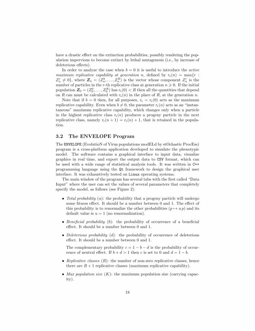
have a drastic effect on the extinction probabilities, possibly rendering the pop-ulation impervious to become extinct by lethal mutagenesis (i.e., by increase ofdeleterious effects).

In order to analyze the case when b = 0 it is useful to introduce the activemaximum replicative capability at generation n, defined by r∗(n) = max{r :Zrn 6= 0}, where Zn = (Z0

n, . . . , ZRn ) is the vector whose component Zrn is the

number of particles in the r-th replicative class at generation n > 0. If the initialpopulation Z0 = (Z0

0 , . . . , ZR0 ) has r∗(0) < R then all the quantities that depend

on R can must be calculated with r∗(n) in the place of R, at the generation n.Note that if b = 0 then, for all purposes, r∗ = r∗(0) acts as the maximum

replicative capability. Even when b 6= 0, the parameter r∗(n) acts as an “instan-taneous” maximum replicative capability, which changes only when a particlein the highest replicative class r∗(n) produces a progeny particle in the nextreplicative class, namely r∗(n + 1) = r∗(n) + 1, that is retained in the popula-tion.

3.2 The ENVELOPE Program

The ENVELOPE (EvolutioN of Virus populations modELd by stOchastic ProcEss)program is a cross-platform application developed to simulate the phenotypicmodel. The software contains a graphical interface to input data, visualizegraphics in real time, and export the output data to CSV format, which canbe used with a wide range of statistical analysis tools. It was written in C++

programming language using the Qt framework to design the graphical userinterface. It was exhaustively tested on Linux operating systems.

The main window of the program has several tabs with the first called “DataInput” where the user can set the values of several parameters that completelyspecify the model, as follows (see Figure 2).

• Total probability (u): the probability that a progeny particle will undergosome fitness effect. It should be a number between 0 and 1. The effect ofthis probability is to renormalize the other probabilities (p 7→ u p) and itsdefault value is u = 1 (no renormalization).

• Beneficial probability (b): the probability of occurrence of a beneficialeffect. It should be a number between 0 and 1.

• Deleterious probability (d): the probability of occurrence of deleteriouseffect. It should be a number between 0 and 1.

The complementary probability c = 1− b− d is the probability of occur-rence of neutral effect. If b+ d > 1 then c is set to 0 and d = 1− b.

• Replicative classes (R): the number of non-zero replicative classes, hencethere are R+ 1 replicative classes (maximum replicative capability).

• Max population size (K): the maximum population size (carrying capac-ity).

18

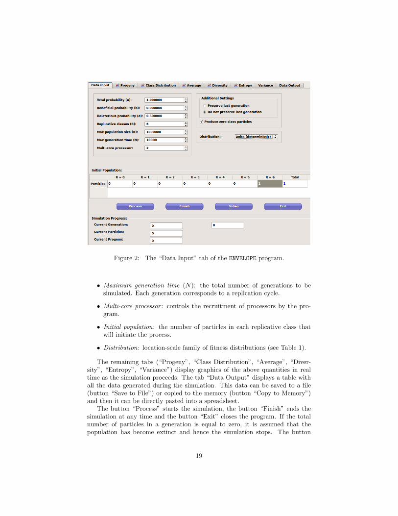
Figure 2: The “Data Input” tab of the ENVELOPE program.

• Maximum generation time (N): the total number of generations to besimulated. Each generation corresponds to a replication cycle.

• Multi-core processor : controls the recruitment of processors by the pro-gram.

• Initial population: the number of particles in each replicative class thatwill initiate the process.

• Distribution: location-scale family of fitness distributions (see Table 1).

The remaining tabs (“Progeny”, “Class Distribution”, “Average”, “Diver-sity”, “Entropy”, “Variance”) display graphics of the above quantities in realtime as the simulation proceeds. The tab “Data Output” displays a table withall the data generated during the simulation. This data can be saved to a file(button “Save to File”) or copied to the memory (button “Copy to Memory”)and then it can be directly pasted into a spreadsheet.

The button “Process” starts the simulation, the button “Finish” ends thesimulation at any time and the button “Exit” closes the program. If the totalnumber of particles in a generation is equal to zero, it is assumed that thepopulation has become extinct and hence the simulation stops. The button

19

Distribution Family (r > 1) Variance

Deterministic tr(k) = δrk 0

Poisson tr(k) = e−r rk

k! r

Geometric tr(k) = 1r+1

(1− 1

r+1

)kr(r + 1)

12 -Binomial tr(k) =

(2rk

)12r r/2

Power law tr(k) = zr(k) +∞

Table 1: Location-scale families of fitness distributions (t0(k) = δ0k always).All distributions are normalized so that the expectation value of tr is r. SeeAppendix B for the definition of the family of distributions zr(k).

“Video” pauses the simulation, without ending the simulation, and allows theuser to change the above parameter settings and continue the simulation withthe new setting. This feature is used to emulate the changes in the environment– the host organism – where the reproduction process takes place.

The evolution of the population can be measured through a few simplequantities that vary as a function of the generation number n > 0. LetZn = (Z0

n, . . . , ZRn ) denote the vector whose component Zrn is the number of

particles in the r-th replicative class at generation n.

• Progeny size: total number of particles |Zn| =∑r Z

rn at generation n.

• Relative growth rate: the relative growth rate at generation n given by(for n > 1)

µ(n) =|Zn||Zn−1|

It is a multidimensional version of the Lotka-Nagaev estimator [64, 76],which gives an empirical estimator of the malthusian parameter.

• Asymptotic distribution of classes: the proportion of particles in the r-threplicative class at generation n given by

ur(n) =Zrn|Zn|

The vector u(n) =(u0(n), . . . , uR(n)

)is called asymptotic distribution of

classes (or simply the class distribution).

• Average reproduction rate: the average reproduction rate (mean of the

20

class distribution) at generation n given by

〈%(n)〉 =

R∑r=0

r ur(n)

It can be shown that the average reproduction rate equals to the relativegrowth rate:

〈%(n)〉 = µ(n) for all n > 1

(see Appendix A for details).

• Phenotypic diversity : the variance (or standard deviation) of the classdistribution at generation n given by

σ2%(n) =

R∑r=0

r2 ur(n)− 〈%(n)〉2

• Phenotypic entropy : the informational or Shannon entropy of the classdistribution at generation n given by

h%(n) = −R∑r=0

ur(n) lnur(n)

Here we use the convention “0 ln 0 ≡ 0”. This quantity behaves very muchlike the phenotypic diversity.

• Normalized populational variance: the normalized populational varianceat generation n given by

φ(n) = σ2(n)− σ2%(n)

where σ2 is the empirical estimator of the variance corresponding to themalthusian parameter µ(n) (see Appendix A for details).

Strictly speaking, a surviving population described by branching processwhich does not becomes extinct grows indefinitely, at an exponential rate pro-portional to µn. Hence, in order to simulate a branching process it is necessaryto impose a cut off on the progeny size, otherwise it would blow up the memoryof the computer. This cut off is done by setting the maximum population sizeK which controls how much the population can grow unconstrained, acting ina similar fashion as the carrying capacity of the logistic growth [13, 60]. If thetotal number of particles that comprises the current generation is greater thanthe maximum population size N , a random sampling procedure is performed tochoose N particles to be used as parental particles for the next generation. Inparticular, the progeny size curve resembles a logistic curve (see Figure 3).

Finally, there are also some other additional settings that alter the way theprogram behaves. “Produce zero class particles” allows to set if the particles

21

of replicative capability r = 0 will be considered in the calculations or not.“Previous last generation/Do not preserve last generation” allows to choose ifthe particles in previous generation will be carried over to current generation.This was included in order to account for the possibility of a replication strat-egy that does not implement the disassemble of the parental particle. In mostcases the replication strategy used by RNA viruses implements the disassem-ble of the virus particle during the replication. Retroviruses replication processis performed by the reverse transcriptase enzyme. The process of reverse tran-scription involves the synthesis of complementary DNA from the single-strandedRNA followed by the degradation of the intermediate RNA-DNA hybrid form.The preservation of the parental generation in the model of viral evolution canallow one or more particle to be preserved during several generations, in contrastwith the above-mentioned replication strategies of the RNA viruses.

4 Consequences of the Phenotypic Model

In this section we explore the phenotypic model in more detail. By combiningfindings obtained by simulation and theoretical arguments based on branchingprocess theory we validate the model at several levels of refinement. The dis-cussion is subdivided into several parts corresponding to distinct features of themodel that are classified according to the possible regimes and phases of thetime evolution of a multitype branching process.

4.1 Transient Phase and Recovery Time

A heterogeneous population replicating in a constant environment typically un-dergoes an initial period of high stochastic fluctuations in the relative frequencyof each variant, until it reaches a stationary regime where the relative frequen-cies become constant. This initial period, called transient phase, is markedby the beginning of the viral infection, after the bottleneck event when one ormore particles are transmitted to a host organism and initiates the process of(re)establishment of the viral population in the new host. The transient phasecomprises the acute infection phase [42, 71], which is characterized by an ini-tial exponential growth of the population, the attainment of the viremia peak,followed by a slower decrease towards a stabilization of the population size (seeFigure 3).

In the phenotypic model the transient regime corresponds to the beginningof the time evolution of the process. It is characterized, as noted before, by aninstability of the relative frequencies of the replicative classes, an exponentialgrowth of the progeny size, a decrease of the average reproduction rate (seethe initial segment of the time series in Figure 4) and an increase of both thephenotypic diversity and the phenotypic entropy. In addition, from observationof the population size time series is not possible to predict what will be theultimate fate of the population (extinction in finite time or indefinite survival).

22

Figure 3: Typical long term behavior of a population with two distinct regimes.The first stage (from n = 0 to n around 10–20) is the transient stage and thesecond stage is the stationary stage. Parameters values: b = 0; d = 0.75; Z8

0 = 1;R = 10; N = 100; K = 106; fitness distribution: Delta.

The expected time (as function of the number of generations) of the relax-ation towards an equilibrium after the bottleneck event, called recovery timemay be naturally expressed in terms of characteristic time derived from the de-cay of the mean auto-correlation function. When the mean auto-correlation, asfunction of the generation number, is of the form exp(−λn) the decay rate isλ and the expected characteristic time to achieve stationarity is 〈Tchar〉 ∼ 1/λ.It can be shown that if µ > 1 then C(n) ≈ exp(− log(µ)n) (see [5]) and henceit follows that 〈Tchar〉 ∼ 1/ log(µ). The dependence of the recovery time onthe initial population is proportional to lnZr∗0 where r∗ is the active maximumreplicative capability of the initial population.

Let us assume, as usual, that the beneficial probability b ≈ 0 and the found-ing population has r∗(0) < R. Then one observes that the progeny size, theaverage reproduction rate, the phenotypic diversity and phenotypic diversitydisplay a time series with several plateaus. The “length” of each plateau is thenumber of generations that the population remains with the same value of r∗(n)and the higher the plateau the longer, on average, is its length. The presence ofa jump indicates that a progeny particle form a parental particle in the replica-tive class r∗(n) has undergone a beneficial effect, that is, the active maximumreplicative capability increases by 1 unit: r∗(n+ 1) = r∗(n) + 1. The occurrenceof jumps can go on until r∗(n) = R. Therefore, the “length” of each plateau

23

Figure 4: Average reproduction rate = Relative growth rate. The “jumps”associated with the recovery time have heights about 0.5. Parameters values:b = 0.000001; d = 0.50; Z5

0 = 1; R = 10; N = 4, 000; K = 106; fitnessdistribution: Delta.

represents the time, in number of generations, required for a beneficial effectto occur on a particle at the highest replicative class and be retained in thepopulation. The probability P

(jump in r∗(n)

)of occurrence of a jump event,

when r∗(n) < R, may be estimated using formula (9) as

P(jump in r∗(n)

)≈ b ur∗(n) ≈ b (1− d)r∗(n)

where ur∗(n) is the proportion of particles in the r∗(n)-th replicative class atgeneration n, which is the active maximum replicative capability at time n.Notice that, as r∗(n) increases, ur∗(n) decreases monotonically and therefore,

P(jump in r∗(n)

)→ 0 when r∗(n) → ∞. This result highlights the asymmetry

between the contributions of the beneficial probability versus the deleteriousprobability to the recovery time.

The “height” of a jump in the average reproduction rate time series is in-dependent of the plateau where the jump occurs. In order to estimate the“height”, consider two consecutive levels on the time series of the average re-production rate, the first “height” µ(n1) measured at generation n1 and thesecond “height” µ(n2) measured at generation n2, with n1 < n2 not necessar-ily consecutive, such that r∗(n2) = r∗(n1) + 1 and µ is approximately constantaround n1 and n2. Thus, the difference µ(n2)− µ(n1) gives an estimate of theheight of the jump between two consecutive plateaus. When b ≈ 0, equation (7)

24

implies that µ(n) ≈ r∗(n)(1− d) and hence

µ(n2)− µ(n1) ≈(r∗(n2)− r∗(n1)

)(1− d) ≈ 1− d .

For instance, in Figure 4 it can be readily seen that the height of the jumps isabout 0.5 and, in fact, d = 0.50, b = 0.000001 and hence 1− d = 0.4999999.

4.2 Stationary Regime

The advanced stage of the infection, also called chronic infection phase [42, 71],is comprised by the stationary regime where the viral population has recoveredits phenotypic (and genotypic) diversity and becomes better adapted to thenew host environment. This regime comes after the end of the transient phasewhen the viral population starts to exhibit a rather stable viral load and thestabilization of the relative frequencies of almost all variants.

In the phenotypic model the stationary regime corresponds to the asymptoticbehavior of a super-critical branching process (µ > 1). But, as mentioned before,a surviving population described by super-critical branching process is neverstationary and therefore this association is not straightforward. Nevertheless,the normalized process Wn = Zn/µ

n is stationary and, when n → ∞, therandom variable Zrn/|Zn| converges to the asymptotic relative frequency ur ofr-th replicative class. Consequently, the average reproduction rate 〈%(n)〉 =µ(n), the phenotypic diversity σ2

%(n) and the phenotypic entropy h%(n) remainessentially constant in time. Moreover, the maximum population size K cut offensures that the total progeny size remains constant in time with expected value〈|Zn|〉 ≈ µ(n)K.

During the stationary regime, the stability of the relative frequency of eachclass is maintained by a steady “flow of particles” from a replicative class to itsadjacent classes, due to the deleterious probability d and the beneficial prob-ability b. The probability c contributes maintenance of a constant proportionof particles in each replicative class. When the beneficial probability b 6= 0 theasymptotic distribution of classes ur is independent of the configuration of thefounding population and, when n is large enough, r∗(n) = R.

More importantly, when b ≈ 0, the replicative classes that are most repre-sentative in the population are the classes near the mode of the distributionof classes ur, also known as “most probable replicative capability”. The modeof ur = binom(r;R, 1 − d) is given by m(ur) = b(R + 1)(1 − d)c, except when(R+ 1)(1− d) happens to be an integer, then the two replicative classes corre-sponding to (R+ 1)(1− d)− 1 and (R+ 1)(1− d) are equally “most probable”(see [40], here, bxc denotes the greatest integer less than x). When (1−d) ≈ 1/2the mode is close to the average reproduction rate µ(n) = 〈%(n)〉 (see Figure 5).

4.3 Threshold of Extinction

The threshold of extinction takes place when the deleterious rate is sufficientlyhigh that it prevents the viral population of reaching the stationary regime but

25

Figure 5: Histogram of the replicative classes. Parameter values: b = 0.000001;d = 0.50; Z5

0 = 1; R = 10; N = 4, 000; K = 106; fitness distribution: Delta.

not high enough to induce the extinction of the population in the short run.Therefore, any small increase in the deleterious rate can push the populationtoward extinction, while any small decrement can allow the population to reachthe stationary regime.

In the phenotypic model, the threshold of extinction corresponds to a criti-cal branching process (µ = 1) and is characterized by instability of the relativefrequencies of the replicative classes, the average replicative rate and the phe-notypic diversity. The instability observed represents the impossibility of theviral population to preserve, due to the deleterious effects, particles with highreplicative capability. The occurrence of an eventual extinction of the popula-tion is almost certain, although the time of occurrence of the extinction may bearbitrarily long if the initial population is sufficiently large. In other words, thethreshold of extinction looks like an infinite transient phase and is the borderlinebetween the stationary regime, where the transient phase ends at an stationaryequilibrium, and the extinction in finite time.

Setting the parameters of the phenotypic model in order to obtain a criticalbranching process is a matter of “fine tuning”, since it requires that the prob-abilities d, b and the maximum replicative capability R satisfy the algebraicequation µ(b, d;R) = 1 – which is a non-generic condition (see Figure 6).

When b = 0, the critical deleterious probability is dc = 1−1/R for each fixedR. When b 6= 0 one may consider the corresponding critical probability dc(b)such that µ(b, dc(b)) = 1. Since b and d are constrained to satisfy b + d 6 1,

26

Figure 6: Progeny size of a population at the extinction threshold. Parametervalues: b = 0; d = 0.50; Z2

0 = 1, 000; R = 2; N = 20, 000; K = 106; fitnessdistribution: Delta.

there is a maximum value of b such that b+ dc(b) = 1 for each fixed R. Denotethis maximum value by b?, that is, b? + dc(b

?) = 1. The critical probabilitiesdc(b

?) can be represented in the parameter space of the phenotypic model as theintersection of the boundary line b+d = 1 with the critical curves µ(d, b, R) = 1for each fixed R.

Using the expressions for the malthusian parameter obtained in [5], it is easyto show that the following approximations hold (when R→∞)

b? ≈ 1

R− 1

R

(R− 1)2

1 + (R− 1)2

dc(b?) ≈ dc(0) +

1

R

(R− 1)2

1 + (R− 1)2.

(14)

Here, one uses that b? +dc(b?) = 1 and dc(0) = 1− 1/R. Comparison of critical

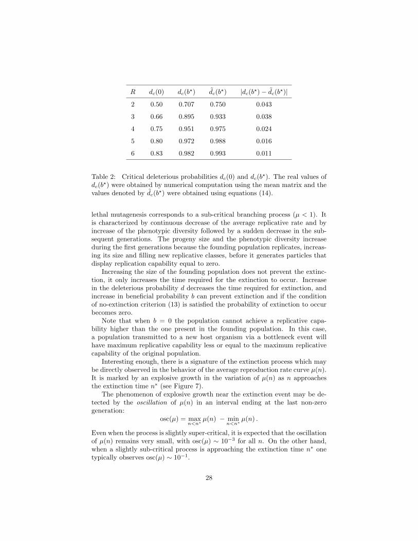
deleterious probability given by equations (14) with the correct values obtainedby numerical computation using the mean matrix, shown in Table 2, indicatethat the asymptotic expressions converge to the real values when R→∞.

4.4 Extinction by Lethal Mutagenesis

The process of extinction of the viral population induced by increase of thedeleterious rate is called lethal mutagenesis [9]. In the phenotypic model, the

27

R dc(0) dc(b?) dc(b

?) |dc(b?)− dc(b?)|

2 0.50 0.707 0.750 0.043

3 0.66 0.895 0.933 0.038

4 0.75 0.951 0.975 0.024

5 0.80 0.972 0.988 0.016

6 0.83 0.982 0.993 0.011

Table 2: Critical deleterious probabilities dc(0) and dc(b?). The real values of

dc(b?) were obtained by numerical computation using the mean matrix and the

values denoted by dc(b?) were obtained using equations (14).

lethal mutagenesis corresponds to a sub-critical branching process (µ < 1). Itis characterized by continuous decrease of the average replicative rate and byincrease of the phenotypic diversity followed by a sudden decrease in the sub-sequent generations. The progeny size and the phenotypic diversity increaseduring the first generations because the founding population replicates, increas-ing its size and filling new replicative classes, before it generates particles thatdisplay replication capability equal to zero.

Increasing the size of the founding population does not prevent the extinc-tion, it only increases the time required for the extinction to occur. Increasein the deleterious probability d decreases the time required for extinction, andincrease in beneficial probability b can prevent extinction and if the conditionof no-extinction criterion (13) is satisfied the probability of extinction to occurbecomes zero.

Note that when b = 0 the population cannot achieve a replicative capa-bility higher than the one present in the founding population. In this case,a population transmitted to a new host organism via a bottleneck event willhave maximum replicative capability less or equal to the maximum replicativecapability of the original population.

Interesting enough, there is a signature of the extinction process which maybe directly observed in the behavior of the average reproduction rate curve µ(n).It is marked by an explosive growth in the variation of µ(n) as n approachesthe extinction time n∗ (see Figure 7).

The phenomenon of explosive growth near the extinction event may be de-tected by the oscillation of µ(n) in an interval ending at the last non-zerogeneration:

osc(µ) = maxn<n∗

µ(n) − minn<n∗

µ(n) .

Even when the process is slightly super-critical, it is expected that the oscillationof µ(n) remains very small, with osc(µ) ∼ 10−3 for all n. On the other hand,when a slightly sub-critical process is approaching the extinction time n∗ onetypically observes osc(µ) ∼ 10−1.

28

Figure 7: Lethal mutagenesis and the path to extinction. Parameter values:b = 0; d = 0.501; R = 2; N = 2, 500; K = 106; Z0 = (1000, 2000, 1000); fitnessdistribution: Delta.

The expected time to extinction 〈Text〉 of a branching process was determinedin [51]: if µ 6 1 then

〈Text〉 =lnZr∗0 + κ

− lnµ

where κ > 0 depends only on the parameters of the model (not on the initialpopulation). It is easy to show that at the critical value of the malthusianparameter (µ = 1) equilibrium is never reached. A scaling exponent charac-terizing the behavior of expected time to extinction in a neighborhood of thecritical value of the malthusian parameter can be obtained by considering thefirst order expansion of 〈Text〉 about 1:

〈Text〉 ∼ |µ− 1|−1 .

When b = 0 one may write 〈Text〉 as a function of the deleterious probabilityand the critical deleterious probability dc = 1− 1/R as

〈Text〉 ∼1

R|d− dc|−1

since |µ − 1| = R|d − dc|. This scaling law is formally identical to the oneobtained in [47] for the error threshold of the deterministic quasispecies modelas a function of the mutation rate.

29

4.5 Finite Population Size and Mutational Meltdown

Recently, Matuszewski et al. [70] reviewed the literature about theories and andmodels describing the extinction of populations owing to the excessive accu-mulation of deleterious mutations or effects and distinguished two apparentlydistinct lines of research, represented by the lethal mutagenesis models [9] andthe mutational meltdown models [66] which, nonetheless, display a considerableamount of similarity.

Indeed, as shown in [9, 4, 5], lethal mutagenesis is independent of populationsize, hence it is fundamentally a deterministic process that operates even on verylarge populations. Although the outcome of lethal mutagenesis is deterministic,other aspects of the population dynamics (such as extinction time, individualtrajectories of progeny size, etc.) are not. On the other hand, the mutationalmeltdown generally works within the context of “small” population sizes inwhich stochastic effects caused by random drift play an important role.

We believe that the approach presented here may help shed some light onthis issue. There is one ingredient in the mutational meltdown theory that isabsent in the lethal mutagenesis theory: the carrying capacity. This is trueeven for models with finite population, such as [23] and the phenotypic model,in their theoretical formulations as branching process. However, as seen before,the computational implementation of the phenotypic model required the intro-duction a cut off K in order to bound the growth of the population. If the cut offis taken as basic constituent of the phenotypic model, and not merely a conve-nient device, then it can play a role similar to a carrying capacity and the modelmay no longer be considered a “pure” branching process, but a self-regulatingbranching process [73, 74].

In a self-regulating branching process not all the offspring produced in agiven generation will to produce offspring in the next generation and hence,it is necessary to introduce a survival probability distribution to stochasticallyregulate the survival of offspring at any generation n as a function of the to-tal population size Tn = |Zn|. The motivation behind this definition is thefollowing: if the population size at a generation n exceeds the carrying capac-ity of the environment then, due to competition for resources, it is less likelythat an offspring produced in that generation will survive to produce offspringat generation n + 1. Let S(n|Tn) denote the conditional probability that anyoffspring produced at generation n survives to produce offspring at generationn+1, given that the population has Tn individuals at generation n. If we definethe conditional probability S as

S(n|Tn) =

{K/Tn if Tn > K1 if Tn 6 K

then the phenotypic model becomes a self-regulating process with carrying ca-pacity K. Moreover, when K → ∞ the self-regulating process reduces to a“pure” branching process. On the other hand, if K is not large enough then akind of random drift effect due to finite population size may take place, whichhappens when the fittest replicative classes are lost by pure chance, since its

30

frequency is typically very low (they are the lesser represented replicative classin the population). If the loss of the fittest replicative class occurs a sufficientnumber of times then the population will undergo extinction. Note that thismay happen even when the process is super-critical, namely, it is far from theextinction threshold. This is not a contradiction, since a super-critical processstill has a positive probability to become extinct.

Now suppose that b = 0, the initial population has active maximum replica-tive capability r∗(0) and the carrying capacity K is sufficiently small (weshall give an estimate of K in a moment). Then, as mentioned before, thevalue r∗ = r∗(0) acts as the maximum replicative capability for that popula-tion. Moreover, if the highest replicative class r∗ is lost by chance, that is, ifr∗(n+1) = r∗(n)−1, then it can not be recovered anymore and hence, from thattime on the maximum replicative capability for that population has dropped by1 unit. This may be seen as a manifestation of the “Muller’s Ratchet”, sincethe population has accumulated a deleterious effect in an irreversible manner.

For sake of concreteness, let us assume that r∗ = R and d are such that(R − 1)(1 − d) < 1, but R(1 − d) > 1. Then, at the beginning of the process,the malthusian parameter is µ = R(1− d) > 1 and the process is super-critical.However, if at some generation n, the R-th replicative class is lost by chance,then R drops by 1 and µ = (R−1)(1−d) < 1, so the process becomes sub-criticaland the population becomes extinct very quickly. In this case, the frequency ofthe R-th replicative class is (1 − d)R and fraction of particles that are purged,at each generation, is R(1−d)−1, hence the fraction of particles that are left inthe R-th replicative class, at each generation, is νR = 2(1− d)R −R(1− d)R+1.If K ≈ 1/νR then there will be, on average, 1 particle of class R per generation– it is very unlikely that this replicative class will be retained for a long periodof time. Therefore, in order to avoid the random drift effect K should be atleast of the order of 10×R(1− d)/νR, or higher.

At each “click of the ratchet” the fittest replicative class is lost and there is adrop in the malthusian parameter by (1−d), until r∗(1−d) becomes less than 1,where r∗ is the maximum replicative capability at the current generation. Thisdrop occurs in the phenotypic diversity and the phenotypic entropy, as well (seeFigure 8).

If one writes the condition for occurrence of extinction r∗(1− d) < 1 as

(1− d) < 1/r∗

then this is a phenotypic version of the mutational meltdown extinction crite-rion, since r∗ is the phenotypic analogue of absolute growth rate of the populationat time n and c = (1−d), the probability of occurrence of a neutral fitness effectper individual particle, is the phenotypic analogue of the mean viability.

4.6 Populational Variance and Fitness Distributions

All properties of the phenotypic model that have been discussed so far are re-lated to the mean matrix of the model, that is, they depend only on the first

31

Figure 8: Extinction by mutational meltdown. Phenotypic Entropy time series.At the beginning the branching process is super-critical with µ = 3.41. Param-eter values: b = 0; d = 0.659; R = 10; N = 10, 000; K = 2, 000; Z10

0 = 6, 000;fitness distributions: Delta.

moments of the branching process and may be called “first order properties”.In particular, they are independent of the choice of the family of fitness distri-butions. If we want to see how the type of fitness distribution influences theevolution of the population we have to look at the “second order properties”of the model, since they are expected to depend on the second moments ofthe fitness distributions, which are distinct among the location-scale families ofdistributions (see Table 1).

The simplest property of second order is given by the population varianceσ2 associated to the malthusian parameter µ (namely, the relative growth rate).Furthermore, the difference between the populational variance and the (squared)phenotypic diversity, called normalized populational variance and denoted by φis a very interesting quantity to be measured, since it satisfies

φ = σ2 − σ2% =

R∑r=0

σ2r ur (15)

In other words, φ is a weighted average of the variances σ2r of the fitness distri-

butions. See Appendix A for the precise definition of σ2 and the proof of thesecond equality in formula (15).

Therefore, given a location-scale family of fitness distributions tr such thatσ2r is at most a quadratic polynomial on r, formula (15) allows one to write

32

the corresponding normalized population variance φ in terms of the averagereproduction rate 〈%〉 and the phenotypic diversity σ2

%. Hence, φ can be exactlycomputed for all location-scale families of distributions used in the ENVELOPE

program (see Table 3).

Distribution σ2r φ

Deterministic 0 0

Poisson r 〈%〉

Geometric r(r + 1) 〈%〉(〈%〉+ 1

)+ σ2

%

12 -Binomial r/2 〈%〉/2

Power law +∞ +∞

Table 3: Location-scale families of fitness distribution of the ENVELOPE program,their variance and the corresponding normalized populational variances.

Assume that b = 0 (then c = 1− d). From the expression of the asymptoticdistribution of classes (8) one obtains: 〈%〉 = µ = R(1− d) and σ2

% = Rd(1− d).Moreover, when b 6= 0 is sufficiently small, formula 9 ensures that 〈%〉 and σ2

%

are approximated by the corresponding values when b = 0 and hence φ mightbe, as well, approximated by the corresponding values listed in Table 3.

For instance, in Figure 9 we show the graph of the normalized populationvariance φ(n), at generation n, from a simulation in which we switched amongthe four families of fitness distributions with finite variance using the “Video”function of the ENVELOPE program to pause the simulation and change the typeof fitness distribution.

Finally, it is worth to remark that the impact of the power law family offitness distribution on the evolution of the population is very distinct from theother families, because, unlike the other fitness distributions, it has infinitevariance.

One of the consequences of this property is the appearance of intense burstsof progeny production clearly seen on the times series of progeny size and theaverage reproduction rate (see Figure 10). The instability caused by unboundedfluctuations coupled with the finite population size effect (even for large K) isresponsible for the generation of a train of sparse and intense bursts of progenyproduction. On the other hand, this instability coupled with finiteness effectmay also provoke sudden drops on the progeny size driving the population to apremature extinction, even if the malthusian parameter is above 1. Because ofthese extreme phenomena one would be led to believe that the phenotypic modelwith the power law family of fitness distributions is an exception to a previousresult saying that any property derived from the mean matrix is independentof the fitness distribution. It is not the case. In fact, if one considers thetime-average of any quantity that is time-dependent over a time interval [n0, N ]

33

Figure 9: Normalized population variance φ, with 〈%〉 = 1 and σ2% = 0.5.

Parameter values: b = 0; d = 0.50; R = 2; N = 2, 000; K = 106; Z20 = 10, 000;

fitness distributions: Delta (φ = 0), Poisson (φ = 1), Geometric (φ = 2.5),Binomial (φ = 0.5).

during the stationary regime, let’s say

µ(N) =1

N

N∑n=n0

µ(n) ,

then it is expected that µ(N) becomes very close to the asymptotic value of therelative growth rate µ when N is sufficiently large. For instance, in Figure 10 thetime-average of the progeny size is around 14, 000, while the expected progenysize for the model is µK = R(1− d)K = 2× 0.7× 104 = 1.4× 104.

5 Conclusion and Outlook

In this paper we have exhaustively explored a phenotypic model for the evo-lution of RNA virus. Our model was formulated as a multivariate branchingprocess. Branching processes provide a theoretical suitable framework endowedwith concepts and tools allowing for the investigation of evolutionary aspects ofRNA viruses propagating along different adaptive landscapes.

One of the greatest virtues of a phenotypic model is its simplicity. By theadoption of only 3 parameters we were to obtain an almost complete quantitativedescription of all possible behaviors of the model. The maximum replication

34

Figure 10: Power law induced bursts (viral blips), with time-average progenysize around 14, 000 viral particles, going up to 400, 000 - 500, 000 particles duringan intense burst. Parameter values: b = 0; d = 0.30; R = 2; N = 5, 000;K = 104; Z2

0 = 10, 000; fitness distribution: Power law.

capacity R and the probabilities of occurrence of deleterious d effects entirelydetermine whether a viral population becomes extinct infinite time or not. Onthe other hand, the third parameter, the probability of occurrence of beneficialeffects b plays a distinct role from the other two probabilities. It works as athreshold parameter classifying the model according to which: (i) the modelhave three regimes of a branching process, or (ii) the model has only the super-critical regime and the population is no longer extinguished.

Besides the many virtues and capability to produce striking results, thephenotypic model has some important drawbacks. The first limitation is thelack of feedback from the host organism on the virus population, since theprobabilities of fitness effects are independent of time. This shortcoming ispartially handled in the ENVELOPE program by the “Video” function, whichallows one to pause the simulation and change the probabilities and emulatethe host’s “response” against the virus. The second limitation is the lack ofthe phenotype-to-genotype map, i.e, the relationship between genotypic andphenotypic change. The motivation to use a phenotypic approach was to avoidthe severe difficulties in modeling this kind of mapping [2, 43].

Although simple, our model allowed us to draw some soft qualitative conclu-sions regarding RNA virus evolution. For example, under the assumption thatthe mutation rate U is sufficiently high (between 0.1 and 1), the probability that

35

a spontaneous mutation produces a deleterious effect may be estimated as fol-lows: if we assume that the number of mutations in a genome follows a Poissondistribution then dsp ≈ 1− e−fd , where fd is the probability that a spontaneousmutation has a deleterious effect [58]. Values of fd have been measured in vitrofor a few viruses and are shown in Table 4, along with the respective mutationrates U .

Virus Group fd dsp U REFS.

VSV (−)ssRNA (V) 0.69 0.50 0.1 [88, 44]

Qβ (+)ssRNA (IV) 0.74 0.52 0.6 [30, 8]

TEV (+)ssRNA (IV) 0.77 0.53 0.5 [14, 93]

Φ6 dsRNA (III) 0.42 0.34 0.03 [11, 12]

ΦX174 ssDNA (II) 0.77 0.53 0.003 [30, 20]

F1 ssDNA (II) 0.65 0.47 0.004 [83, 32]

Table 4: Measured values of fd, the corresponding deleterious probabilitydsp = 1− e−fd and genome-wide spontaneous mutation rate U .

Now, dsp provides a lower bound for the deleterious probability and sincethe value dsp ≈ 1/2 seems to be typical for RNA viruses, the interval 1/2 <d < dc = 1− 1/R is more likely to be the range of the parameter d. Moreover,it is easy to see that the phenotypic diversity and the phenotypic entropy aremaximal when d is near 1/2, for any value of R [4]. One could speculate thatthis is a universal property for RNA viruses that replicate under high mutationalrates associated to a maximization principle that seeks to improve the chancesof survival.

Maintenance of high mutation rates makes it difficult for a population to re-tain its fittest replicative classes. As a consequence, the most adapted replicativeclasses are not usually the ones most represented in a RNA virus the population.Indeed, when b ≈ 0, the distribution of classes ur is approximately a binomialdistribution. Hence, the most frequent replicative classes in the population arethe ones whose replicative capability is near the mode of ur, also known as “mostprobable replicative capability”. This behavior may be seen as a manifestationof the “Survival of the Flattest” phenomenon [98].

According to the phenotypic model – as long as the probabilities for fitnesseffects remain constant – the maximum replicative capability R determines thesuccess of an incoming virus population because the corresponding criticalitythreshold is uniquely determined by R. This observation suggests that minimuminnoculums must have at least one particle with a sufficiently high replicativecapability. It has been shown that only a limited number of particles, and insome cases even one particle, is enough to start a new infectious process ina host [52, 84, 100]. We speculate that those particles with sufficiently high

36

replicative capability should constitute the effective innoculum of [100]. In fact,the experimental data about HIV innocculums have shown that the majority ofpatients are infected by a single virus particles and others started their infectionswith 1 to 5 particles [52, 84].

By a meticulous exploration of the parameter space we were able to uncoverits “generic behaviors”, which are the most likely the outcomes of the modelsdynamics. We show that the establishment of a virus population may displayfour distinct phases/regimes: (i) transient phase, (ii) stationary regime, (iii)threshold of extinction, (iv) extinction in finite time. The transient phase cor-responds to the beginning of the models evolution and when this phase is overany one of the other three regimes can take place, according to the values of d,b and R. One of the main results of the model is the identification of a unifyingprinciple tied to the probability of occurrence of deleterious effects d and themaximum replicative capability R. These are essentially the main forces thatdrive a RNA virus population into its own extinction. Based on this unify-ing principle we show that there is a correspondence between the two principalmechanisms leading RNA viruses populations into extinction: lethal mutage-nesis and mutational meltdown. Therefore, as far as the phenotypic model isconcerned, this result is a proof of the claim [70] that these two mechanisms are“two sides of the same coin”.

The addition of fitness distributions to the model was motivated by the re-sults and observations made by authors [99] on the distribution of single cellprogeny sizes of RNA viruses. In their study the authors demonstrated thateven in a most controlled experiment, using the same viral isolate, same infectionparameters and clonally expanded target cells, progeny sizes can vary substan-tially. The variance on progeny sizes in such uniform environment indicates thatRNA viruses replication bears in some way a portion of unpredictability. In thismanner, it is impossible to know how many particles will be produced by a celluntil the infection takes place and the progeny is released. So including fitnessdistributions to the model was a way to accommodate the unpredictability toeach viral replication cycle. In our model each viral replicative class has a meanprogeny size. However,different fitness distributions will allow the occurrenceof large or smaller progenies within a single replicative class at the same timepreserving the mean progeny size of this class. If in a fitness distribution repli-cation events leading to above the median progeny size take place, this fitnessdistribution is thought to be favorable for the virus. On the contrary, fitnessdistributions with frequent bellow the median progeny sizes are unfavorable forvirus. In a different way of saying, fitness distributions could represent distinct“compartments” in which viruses are replicating inside the host organism. Asmentioned before, the heterogeneous nature of the host environment displayssites more favorable or unfavorable for the virus. So these distributions act as theenvironmental component having an impact on the evolution of RNA viruses.In fact according to our model, some types of fitness distributions may havea substantial consequence on the evolution of viruses, most notably the powerlaw. The extreme behavior produced by the power law shown in Figure 10 re-sembles that of the “viral load blips” frequently observed in HIV patients under

37

highly active antiretroviral therapy (HAART) [25, 78, 77, 62, 45, 87, 86] withundetectable or low viral loads. This particular prediction of the model agreeswith the suggestion that these events are purely random fluctuations since viralloads blips return to basal load values soon after their occurrence.

Finally, during the modeled viral evolution process presented here we haveconsidered three types of fitness effects; the deleterious, beneficial and neutral.By doing this, our model was kept simple and the computational simulationscan be easily handled and analyzed by different users. However, fitness effectsrepresent a broad group forces acting on virus replication and one direction forfurther investigation would be to ungroup some of these forces and test them.For example, on the deleterious side, the inclusion of defective interfering par-ticles could yield a particular extinction mechanism, whereas on the beneficialside, the inclusion of recombination could help the viral population escape fromextinction.

Acknowledgments. LG acknowledges the support of FAPESP through thegrant 14/13382-1. BG and DC received financial support from CAPES.

Software Availability and Requirements. The ENVELOPE program waswritten in C++ programming language, using the Qt 4.8.6 framework, with theQwt 5.2.1 library. It runs on Linux operating system and requires at least2 GB of RAM memory and 1.5 MB of disk space. Its distribution is free toall users under the LGPL license. Binary files for Linux and MAC OS X areavailable for download at: https://envelopeviral.000webhostapp.com

Author contribution: LG and DC contributed equally to this work. LMRJand FA contributed equally to this work. Conceived the model and formulatedthe underlying theory: LMJR and FA. Implemented the software: LG, DC andBG. Simulated the model and analyzed the output: LG and DC. Wrote thepaper: LMRJ and FA.

Appendices

A Asymptotic Behavior of Supercritical Multi-type Branching Processes

When a multitype branching process is super-critical it is expected that, accord-ing to the “Malthusian Law of Growth” it will grow indefinitely at a geometricrate proportional to µn, where µ is the malthusian parameter,

Zn ≈ µnWn

for some bounded random vector Wn, when n → ∞. The formalization ofthis heuristic reasoning is called Kesten-Stigum limit theorem for super-critical

38

multitype branching processes (see [55, 54, 56]). If Wn = Zn/µn then there

exists a scalar random variable W 6= 0 such that, with probability one,

limn→∞

Wn = W u (16)

where u is the right eigenvector corresponding to the malthusian parameter µand

E(W |Z0) = vtZ0 (17)

where v is the left eigenvector corresponding to the malthusian parameter µ.The vectors u and v may be normalized so that

vtu = 1 and 1tu = 1

where t denotes the transpose of a vector. Moreover, under very general assump-tions on M , that are satisfied by the mean matrix of the phenotypic model (5),the right and left eigenvectors corresponding to the malthusian parameter arenon-negative.

The normalization of right eigenvector u = (u0, . . . , uR) implies that∑r ur = 1 and therefore by the “convergence of types” (see [59])

limn→∞

Zn|Zn|

= u , (18)

where |Zn| =∑r Z

rn is the total population at the n-th generation and the equal-

ity holds almost surely. Equation (18) asserts that the asymptotic proportionof a replicative class r converges almost surely to the constant value ur.

In particular, equation (18) implies that the malthusian parameter is theasymptotic relative growth rate of the population

µ = limn→∞

|Zn||Zn−1|

= limn→∞

1

|Zn−1|

|Zn−1|∑j=1

#[ j ] (19)

since |Zn−1| may be interpreted as the set of “parental particles” of the particlesin the n-th generation and |Zn| is the sum of the “progeny sizes” #[ j ] of the“parental particles” j from the previous generation.

Now consider the quantitative random variable % defined on the set of replica-tive classes {0, . . . , R} and having probability distribution (u0, . . . , uR), calledthe asymptotic distribution of classes. Since the replicative classes are indexedby their expectation values the variable % associates to a random viral particleits expected replicative class

P(% = r) = ur .

Therefore, one can define the average reproduction rate of the population as

〈%〉 =

R∑r=0

r ur . (20)

39

Using equations (16), (17), (18) one can show that the average reproductionrate is equal to the malthusian parameter:

〈%〉 = µ . (21)

The average population size at the n-th generation is |〈Zn〉| =∑Rr=0〈Zrn〉. Then

for n→∞, equation (16) gives |〈Zn〉| ≈ µn|〈Wn〉| ≈ µn〈W 〉 and so

µ = limn→∞

|〈Zn〉||〈Zn−1〉|

(22)

On the other hand, from the definition of mean matrix and its form (5), one has

|〈Zn〉| = |M 〈Zn−1〉| =R∑r=0

r 〈Zrn−1〉 .

Now dividing by |〈Zn−1〉| and taking the limit n→∞ gives

µ = limn→∞

|〈Zn〉||〈Zn−1〉|

= limn→∞

R∑r=0

r〈Zrn−1〉|〈Zn−1〉|

=

R∑r=0

r ur = 〈%〉

where here we used equations (17) and (18) in the third equality from left toright.

In analogy with the characterization of the malthusian parameter as givenby equation (19) we define the asymptotic populational variance

σ2 = limn→∞

1

|Zn−1|

|Zn−1|∑j=1

#[ j ]2 − µ2 (23)

and in analogy with the mean reproduction rate we define the (squared) pheno-typic diversity as

σ2% = 〈%2〉 − 〈%〉2 (24)

By decomposing the sum in equation (23) according to the replicative classesone obtains

|Zn−1|∑j=1

#[ j ]2 =

R∑r=0

Zrn−1∑jr=1

#[ jr ]2

where jr runs over the particles of class r for r = 0, . . . , R and #[ jr ] areindependent random variables with distribution tr.

Now, denoting the variance of the fitness distribution tr by σ2r , we can rewrite

40

the limit in equation (23) as

σ2 = limn→∞

1

|Zn−1|

|Zn−1|∑j=1

#[ j ]2 − µ2

= limn→∞

1

|Zn−1|

R∑r=0

Zrn−1 1

Zrn−1

Zrn−1∑jr=1

#[ j ]2 − r2+ Zrn−1

− µ2

= limn→∞

1

|Zn−1|

R∑r=0

(σ2r + r2)Zrn−1 − µ2

Then equations (18), (21) and (24) give

σ2 =

R∑r=0

(σ2r + r2)ur − µ2 =

R∑r=0

σ2r ur + σ2

% (25)

The difference between the asymptotic populational variance and the (squared)phenotypic diversity, called normalized populational variance, is the weightedaverage of the variances of the fitness distributions

φ = σ2 − σ2% =

R∑r=0

σ2r ur . (26)

In particular, when the family of fitness distributions is deterministic the pop-ulational variance is the same as the phenotypic diversity and φ = 0. This isan expected result since the Delta distributions tr(k) = δrk have variance 0 andhence the only source of fluctuation of the population size is due to its stratifi-cation into replicative classes, which is expressed by the phenotypic diversity.

Unlike the malthusian parameter, the normalized populational variance doesdepend on the choice of the family of fitness distributions. Recall that themalthusian parameter depends only on the mean matrix, which depends onthe fitness distributions tr only through its expectation values. Since we haveimposed the same normalization condition that the expectation value of tr is rfor all families of fitness distributions, it follows that the mean matrix, and hencethe malthusian parameter, does not depend on the family of fitness distributions.On the other hand, the variances of different families of fitness distributions arenot necessarily the same. For instance, if tr is the family of Poisson distributionsthen σ2

r = r and thus φ = µ.

B Power Law Distribution Family

It is typical to parameterize power law distributions by the exponent s, whichmeasures the “weight of the tail” of the distribution. However, we need to havea location-scale parameterized family in order to impose the same normalization

41

as we have done for the other types of distributions. Therefore, we define thepower law distribution with mean value r by

zr(k) =(k − 1)s(r)

ζ(s(r))

for k = 0, 1, . . . ,∞ and r > 1, where ζ(s) is the Riemann zeta function, definedfor s > 1, by

ζ(s) =

∞∑n=1

1

ns

and the function s(r) is given by the inverse function of

r = ϕ(s) =ζ(s− 1)

ζ(s)− 1 .

Namely, s = ϕ−1(r) for r > 1 and hence when 1 6 r < ∞ the exponent ssatisfies 3 < s < 2. Moreover, the Laurent series expansion for r →∞ (s→ 2)is given by:

s(r) ≈ 2 +6

π2(1 + r − C). (27)

The constant C in the previous formula is given by

C =6γπ2 − 36 ζ ′(2)

π4≈ 0.6974

where γ is Euler’s constant and ζ ′(2) is the derivative of ζ(s) evaluated at 2.Observe that when the mean value r > 1, the exponent s < 3, which meansthat the variance of zr(k) is infinite.

The implementation of the pseudo-random generation of samples from thedistribution zr(k) in the ENVELOPE program is based on the algorithm of [24] forthe Zipf distribution on the positive integers, using formula 27 for the compu-tation of the exponent s given the mean value r. Pseudo-random generation forthe remaining fitness distributions were implemented using the standard libraryof C++ programing language (this library requires C++ (2011) or superior).

References

[1] M. E. Abram, A. L. Ferris, W. Shao, W. G. Alvord, and S. H. Hughes.Nature, position, and frequency of mutations made in a single cycle ofHIV-1 replication. J. Virology, 84(19):9864–9878, 2010.

[2] P. Alberch. From genes to phenotype: dynamical systems and evolvability.Genetica, 84(1):5–11, 1991.

[3] J. P. Anderson, Richard Daifuku, and Lawrence A Loeb. Viral errorcatastrophe by mutagenic nucleosides. Annu. Rev. Microbiol., 58:183–205, 2004.

42

[4] F. Antoneli, F. A. R. Bosco, D. Castro, and L. M. R. Janini. Viralevolution and adaptation as a multivariate branching process. In R. P.Mondaini, editor, BIOMAT 2012 – Proceedings of the International Sym-posium on Mathematical and Computational Biology, volume 13, pages217–243. World Scientific, 2013.

[5] F. Antoneli, F. A. R. Bosco, D. Castro, and L. M. R. Janini. Virusreplication as a phenotypic version of polynucleotide evolution. Bulletinof Mathematical Biology, 75(4):602–628, 2013.

[6] K. B. Athreya and P. E. Ney. Branching Processes. Springer-Verlag,Berlin, 1972.

[7] Carl T Bergstrom, Paul McElhany, and Leslie A Real. Transmission bot-tlenecks as determinants of virulence in rapidly evolving pathogens. Pro-ceedings of the National Academy of Sciences, 96(9):5095–5100, 1999.

[8] K. Bradwell, M. Combe, P. Domingo-Calap, and R. Sanjuan. Correlationbetween mutation rate and genome size in riboviruses: mutation rate ofbacteriophage Qβ. Genetics, 195(1):243–251, 2013.

[9] J. J. Bull, R. Sanjuan, and C. O. Wilke. Theory of lethal mutagenesis forviruses. J. Virology, 18(6):2930–2939, 2007.

[10] J. J. Bull, R. Sanjuan, and C. O. Wilke. Lethal mutagenesis. InE. Domingo, C. R. Parrish, and J. J. Holland, editors, Origin and Evo-lution of Viruses, chapter 9, pages 207–218. Academic Press, London,second edition edition, 2008.

[11] C. L. Burch and L. Chao. Epistasis and its relationship to canalization inthe rna virus Φ6. Genetics, 167(2):559–567, 2004.

[12] C. L. Burch, S. Guyader, D. Samarov, and H. Shen. Experimental estimateof the abundance and effects of nearly neutral mutations in the rna virusΦ6. Genetics, 176(1):467–476, 2007.

[13] R. B. Campbell. A logistic branching process for population genetics.Journal of Theoretical Biology, 225(2):195–203, 2003.

[14] P. Carrasco, F. de la Iglesia, and S. F. Elena. Distribution of fitness andvirulence effects caused by single-nucleotide substitutions in Tobacco EtchVirus. J. Virology, 18(23):12979–12984, 2007.

[15] R. Cerf and J. Dalmau. The distribution of the quasispecies for a moranmodel on the sharp peak landscape. Stochastic Processes and their Appli-cations, 126(6):1681–1709, 2016.

[16] B. Charlesworth. Evolution in age-structured populations, volume 2. Cam-bridge University Press Cambridge, Cambridge, UK, 1994.

43

[17] H. Y. Chen, M. Di Mascio, A. S. Perelson, D. D. Ho, and L. Zhang.Determination of virus burst size in vivo using a single-cycle siv in rhesusmacaques. Proc. Natl. Acad. Sci. U. S. A., 104(48):19079–19084, 2007.

[18] S. Crotty, C. E. Cameron, and R. Andino. RNA virus error catastrophe:direct molecular test by using ribavirin. Proc. Natl. Acad. Sci. U. S. A.,98:6895–6900, 2001.

[19] J. A. Cuesta. Huge progeny production during transient of a quasi-speciesmodel of viral infection, reproduction and mutation. Math. Comp. Model.,54:1676–1681, 2011.

[20] J. M. Cuevas, S. Duffy, and R. Sanjuan. Point mutation rate of bacterio-phage ΦX174. Genetics, 183:747–749, 2009.

[21] J. Dalmau. The distribution of the quasispecies for the wright–fisher modelon the sharp peak landscape. Stochastic Processes and their Applications,125(1):272–293, 2015.

[22] J. Dalmau. Distribution of the quasispecies for a galton–watson process onthe sharp peak landscape. Journal of Applied Probability, 53(02):606–613,2016.

[23] L. Demetrius, P. Schuster, and K. Sigmund. Polynucleotide evolution andbranching processes. Bull. Math. Biol., 47(2):239–262, 1985.

[24] L. Devroye. Non-Uniform Random Variate Generation. Springer-Verlag,1986.

[25] M. Di Mascio, M. Markowitz, M. Louie, C. Hogan, A. Hurley, C. Chung,D. D. Ho, and A. S. Perelson. Viral blip dynamics during highly activeantiretroviral therapy. Journal of Virology, 77(22):12165–12172, 2003.

[26] E. Domingo and J. J. Holland. Rna virus mutations and fitness for sur-vival. Annual Reviews in Microbiology, 51(1):151–178, 1997.

[27] E. Domingo, V. Martin, C. Perales, A. Grande-Perez, J. Garcia-Arriaza,and A. Arias. Viruses as quasispecies: biological implications. In Qua-sispecies: Concept and Implications for Virology, pages 51–82. Springer,2006.

[28] E. Domingo, E. Martınez-Salas, F. Sobrino, J. C. de la Torre, A. Portela,J. Ortın, C. Lopez-Galindez, P. Perez-Brena, N. Villanueva, andR. Najera. The quasispecies (extremely heterogeneous) nature of viralRNA genome populations: biological relevance – a review. Gene, 40(1):1–8, 1985.

[29] E. Domingo, D. Sabo, T. Taniguchi, and G. Weissmann. Nucleotide se-quence heterogeneity of an rna phage population. Cell, 13:635–744, 1978.

44

[30] P. Domingo-Calap, J. M. Cuevas, and R. Sanjuan. The fitness effectsof random mutations in single-stranded DNA and RNA bacteriophages.PLoS Genet, 5(11):e1000742, 2009.

[31] J. W. Drake. Rates of spontaneous mutation among RNA viruses. Proc.Natl. Acad. Sci. U. S. A., 90(9):4171–4175, 1993.

[32] J. W. Drake. A test of Kimura’s mutation-rate conjecture. In Radiobiologyand Environmental Security, pages 13–18. Springer, 2012.

[33] J. W. Drake, B. Charlesworth, D. Charlesworth, and J. F. Crow. Ratesof spontaneous mutation. Genetics, 148(4):1667–1686, 1998.

[34] J. W. Drake and J. J. Holland. Mutation rates among RNA viruses. Proc.Natl. Acad. Sci. U. S. A., 96:13910–13913, 1999.

[35] S. Duffy, L. A. Shackelton, and E. C. Holmes. Rates of evolutionarychange in viruses: patterns and determinants. Nature Reviews Genetics,9(4):267–276, 2008.

[36] M. Eigen. Selforganization of matter and the evolution of biological macro-molecules. Naturwissenschaften, 58:465–523, 1971.

[37] M. Eigen. Viral quasispecies. Sci. Am., 269:42–49, 1993.

[38] M. Eigen and P. Schuster. The Hypercycle. A principle of natural self-organization. Springer-Verlag, Berlin, 1979.

[39] A. Eyre-Walker and P. D. Keightley. The distribution of fitness effects ofnew mutations. Nat. Rev. Genet., 8(8):610–618, Aug 2007.

[40] W. Feller. An Introduction to Probability Theory and Its Applications,volume 1. Wiley, New York, third edition, 1968.

[41] J. Felsenstein. The evolutionary advantage of recombination. Genetics,78(2):737–756, 1974.

[42] E. W. Fiebig, D. J. Wright, B. D. Rawal, P. E. Garrett, R. T. Schumacher,L. Peddada, C. Heldebrant, R. Smith, A. Conrad, S. H. Kleinman, andM. P. Busch. Dynamics of hiv viremia and antibody seroconversion inplasma donors: implications for diagnosis and staging of primary hiv in-fection. Aids, 17(13):1871–1879, 2003.

[43] M. A. Fortuna, L. Zaman, C. Ofria, and A. Wagner. The genotype-phenotype map of an evolving digital organism. PLoS computational bi-ology, 13(2):e1005414, 2017.

[44] V. Furio, A. Moya, and R. Sanjuan. The cost of replication fidelity in anrna virus. Proceedings of the National Academy of Sciences of the UnitedStates of America, 102(29):10233–10237, 2005.

45

[45] J. E. Gallant. Making sense of blips. Journal of Infectious Diseases,196(12):1729–1731, 2007.

[46] S. Gavrilets. Fitness Landscapes and the Origin of Species. PrincetonUniversity Press, 2004.

[47] V. Gupta and N. M. Dixit. Scaling law characterizing the dynamics of thetransition of HIV-1 to error catastrophe. Physical biology, 12(5):054001,2015.

[48] T.E. Harris. The Theory of Branching Processes. Springer-Verlag, Berlin,1963.

[49] J. J. Holland, K. Spindler, F. Horodyski, E. Grabau, S. Nichol, and S. Van-dePol. Rapid evolution of RNA genomes. Science, 215(4540):1577–1585,1982.

[50] M. Imhof and C. Schlotterer. Fitness effects of advantageous mutationsin evolving Escherichia coli populations. Proc. Natl. Acad. Sci. U. S. A.,98(3):1113–1117, Jan 2001.

[51] P. Jagers, F. C. Klebaner, and S. Sagitov. On the path to extinction.Proc. Natl. Acad. Sci. U. S. A., 104(15):6107–6111, April 2007.

[52] B. F. Keele, E. E. Giorgi, J. F. Salazar-Gonzalez, J. M. Decker,K. T. Pham, M. G. Salazar, C. Sun, T. Grayson, S. Wang, H. Li,X. Wei, C. Jiang, J. L. Kirchherr, F. Gao, J. A. Anderson, L.-H. Ping,R. Swanstrom, G. D. Tomaras, W. A. Blattner, P. A. Goepfert, J. M.Kilby, M. S. Saag, E. L. Delwart, M. P. Busch, M. S. Cohen, D. C. Mon-tefiori, B. F. Haynes, B. Gaschen, G. S. Athreya, H. Y. Lee, N. Wood,C. Seoighe, A. S. Perelson, T. Bhattacharya, B. T. Korber, B. H. Hahn,and G. M. Shaw. Identification and characterization of transmitted andearly founder virus envelopes in primary HIV-1 infection. Proc. Natl.Acad. Sci. U. S. A., 105(21):7552–7557, 2008.

[53] P. D. Keightley and M. Lynch. Toward a realistic model of mutationsaffecting fitness. Evolution, 57(3):683–685; discussion 686–689, Mar 2003.

[54] H. Kesten and B. P. Stigum. Additional limit theorems for indecomposablemultidimensional Galton-Watson processes. Ann. Math. Stat., 37(6):1463–1481, 1966.

[55] H. Kesten and B. P. Stigum. A limit theorem for multidimensional Galton-Watson processes. Ann. Math. Stat., 37(5):1211–1223, 1966.

[56] H. Kesten and B. P. Stigum. Limit theorems for decomposable multi-dimensional Galton-Watson processes. J. Math. Anal. Appl., 17:309–338,1967.

46

[57] M. Kimmel and D.E. Axelrod. Branching Processes in Biology. Springer-Verlag, New York, 2002.

[58] M. Kimura and T. Maruyama. The mutational load with epistatic geneinteractions in fitness. Genetics, 54(6):1337, 1966.

[59] T. G. Kurtz, R. Lyons, R. Pemantle, and Y. Peres. A conceptual proofof the Kesten-Stigum theorem for multi-type branching processes. InK. Athreya and P. Jagers, editors, Classical and Modern Branching Pro-cesses, volume 84 of IMA Vol. Math. Appl., pages 181–185. Springer-Verlag, New York, 1994.

[60] A. Lambert. The branching process with logistic growth. The Annals ofApplied Probability, 15(2):1506–1535, 2005.

[61] A. S. Lauring, J. Frydman, and R. Andino. The role of mutational robust-ness in RNA virus evolution. Nature Reviews Microbiology, 11(5):327–336,2013.

[62] P. K. Lee, T. L. Kieffer, R. F. Siliciano, and R. E. Nettles. HIV-1 viralload blips are of limited clinical significance. Journal of AntimicrobialChemotherapy, 57(5):803–805, 2006.

[63] P. H. Leslie. The intrinsic rate of increase and the overlap of successivegenerations in a population of guillemots (uria aalge pont.). Journal ofAnimal Ecology, 35(2):291–301, 1966.

[64] A. J. Lotka. Theorie analytique des associations biologiques. part ii. anal-yse demographique avec application particuliere al’espece humaine. Actu-alites Scientifiques et Industrielles, 780:123—136, 1939.

[65] M. Lynch, R. Burger, D. Butcher, and W. Gabriel. The mutational melt-down in asexual populations. Journal of Heredity, 84(5):339–344, 1993.

[66] M. Lynch and W. Gabriel. Mutation load and the survival of small pop-ulations. Evolution, pages 1725–1737, 1990.

[67] J. M. Malpica, A. Fraile, I. Moreno, C. I. Obies, J. W. Drake, andF. Garcıa-Arenal. The rate and character of spontaneous mutation inan rna virus. Genetics, 162(4):1505–1511, 2002.

[68] S. C. Manrubia, E. Lazaro, J. Perez-Mercader, C. Escarmıs, andE. Domingo. Fitness distributions in exponentially growing asexual pop-ulations. Phys. Rev. Lett., 90(18):188102, 2003.

[69] L. M. Mansky and H. M. Temin. Lower in vivo mutation rate of HumanImmunodeficiency Virus type 1 than that predicted from the fidelity ofpurified reverse transcriptase. J. Virology, 69(8):5087–5094, 1995.

47

[70] S. Matuszewski, L. Ormond, C. Bank, and J. D. Jensen. Two sides of thesame coin: A population genetics perspective on lethal mutagenesis andmutational meltdown. Virus Evolution, 3(1), 2017.

[71] A. J. McMichael, P. Borrow, G. D. Tomaras, N. Goonetilleke, and B. F.Haynes. The immune response during acute hiv-1 infection: clues forvaccine development. Nature Reviews Immunology, 10(1):11–23, 2010.

[72] R. Miralles, P. J. Gerrish, A. Moya, and S. F. Elena. Clonal interferenceand the evolution of RNA viruses. Science, 285(5434):1745–1747, Sep1999.

[73] C. J. Mode and C. K. Sleeman. Stochastic processes in genetics and evo-lution: computer experiments in the quantification of mutation and selec-tion. World Scientific, 2012.

[74] C. J. Mode, C. K. Sleeman, and T. Raj. On the inclusion of self regu-lating branching processes in the working paradigm of evolutionary andpopulation genetics. Frontiers in Genetics, 4, 2013.

[75] H. J. Muller. The relation of recombination to mutational advance. Mutat.Res., 106:2–9, May 1964.

[76] A. V. Nagaev. On estimating the expected number of direct descendants ofa particle in a branching process. Theory of Probability & Its Applications,12(2):314–320, 1967.

[77] R. E. Nettles and T. L. Kieffer. Update on HIV-1 viral load blips. CurrentOpinion in HIV and AIDS, 1(2):157–161, 2006.

[78] R. E. Nettles, T. L. Kieffer, P. Kwon, D. Monie, Y. Han, T. Parsons,J. Cofrancesco, J. E. Gallant, T. C. Quinn, and B. Jackson. IntermittentHIV-1 viremia (blips) and drug resistance in patients receiving HAART.Jama, 293(7):817–829, 2005.

[79] P. K. O’Neil, G. Sun, H. Yu, Y. Ron, J. P. Dougherty, and B. D. Pre-ston. Mutational analysis of HIV-1 long terminal repeats to explore therelative contribution of reverse transcriptase and RNA polymerase II toviral mutagenesis. Journal of Biological Chemistry, 277(41):38053–38061,2002.

[80] H. A. Orr. The distribution of fitness effects among beneficial mutations.Genetics, 163(4):1519–1526, Apr 2003.

[81] M. Parera, G. Fernandez, B. Clotet, and M. A. Martınez. HIV-1 proteasecatalytic efficiency effects caused by random single amino acid substitu-tions. Mol. Biol. Evol., 24(2):382–387, Feb 2007.

[82] N. Pariente, S. Sierra, P. R. Lowenstein, and E. Domingo. Efficient virusextinction by combinations of a mutagen and antiviral inhibitors. Journalof Virology, 75(20):9723–9730, 2001.

48

[83] J. B. Peris, P. Davis, J. M. Cuevas, M. R. Nebot, and R. Sanjuan. Distri-bution of fitness effects caused by single-nucleotide substitutions in bac-teriophage F1. Genetics, 185(2):603–609, 2010.

[84] R. M. Ribeiro, L. Qin, L. L. Chavez, D. Li, S.G. Self, and A. S. Perelson.Estimation of the initial viral growth rate and basic reproductive numberduring acute HIV-1 infection. J. Virology, 84(12):6096–6102, Jun 2010.

[85] D. R. Rokyta, C. J. Beisel, P. Joyce, M. T. Ferris, C. L. Burch, and H. A.Wichman. Beneficial fitness effects are not exponential for two viruses. J.Mol. Evol., 67(4):368–376, Oct 2008.

[86] L. Rong and A. S. Perelson. Asymmetric division of activated latently in-fected cells may explain the decay kinetics of the hiv-1 latent reservoir andintermittent viral blips. Mathematical Biosciences, 217(1):77–87, 2009.

[87] L. Rong and A. S. Perelson. Modeling hiv persistence, the latent reservoir,and viral blips. Journal of Theoretical Biology, 260(2):308–331, 2009.

[88] R. Sanjuan, A. Moya, and S. F. Elena. The distribution of fitness effectscaused by single-nucleotide substitutions in an RNA virus. Proc. Natl.Acad. Sci. U. S. A., 101:8396–8401, 2004.

[89] R. Sanjuan, M. R. Nebot, N. Chirico, L. M. Mansky, and R. Belshaw.Viral mutation rates. J. Virology, 84(19):9733–9748, 2010.

[90] M. R. Servedio, Y. Brandvain, S. Dhole, C. L. Fitzpatrick, E. E. Gold-berg, C.A. Stern, J. V. Cleve, and D. J. Yeh. Not just a theory –the utility of mathematical models in evolutionary biology. PLoS Biol.,12(12):e1002017, 2014.

[91] D. A. Steinhauer and J. J. Holland. Rapid evolution of RNA viruses.Annual Reviews in Microbiology, 41(1):409–431, 1987.

[92] N. Takeuchi and P. Hogeweg. Error-threshold exists in fitness landscapeswith lethal mutants. BMC Evolutionary Biology, 7(1):15, 2007.

[93] N. Tromas and S. F. Elena. The rate and spectrum of spontaneous mu-tations in a plant RNA virus. Genetics, 185(3):983–989, 2010.

[94] E. Van Nimwegen, J. P. Crutchfield, and M. Huynen. Neutral evolution ofmutational robustness. Proc. Natl. Acad. Sci. U. S. A., 96(17):9716–9720,1999.

[95] G. P. Wagner and P. Krall. What is the difference between models oferror thresholds and muller’s ratchet? Journal of Mathematical Biology,32(1):33–44, 1993.

[96] H. W. Watson and F. Galton. On the probability of the extinction offamilies. J. Anthropol. Inst. Great Britain and Ireland, 4:138–144, 1874.

49

[97] C. O. Wilke. Quasispecies theory in the context of population genetics.BMC Evolutionary Biology, 5(1):44, 2005.

[98] C. O. Wilke, J. L. Wang, C. Ofria, R.E Lenski, and C. Adami. Evolutionof digital organisms at high mutation rates leads to survival of the flattest.Nature, 412(6844):331–333, Jul 2001.

[99] Y. Zhu, A. Yongky, and J. Yin. Growth of an RNA virus in single cellsreveals a broad fitness distribution. Virology, 385(1):39–46, Mar 2009.

[100] M. P. Zwart, J.-A. Daros, and S. F. Elena. One is enough: In vivo effectivepopulation size is dose-dependent for a plant RNA virus. PLoS Pathog,7(7):e1002122, 2011.

50