Embed Size (px)
Citation preview

TEL AVIV UNIVERSITYTHE RAYMOND AND BEVERLY SACKLER FACULTY OF EXACT SCIENCES
Department of Applied Mathematics
STOCHASTIC MODEL OF
A PENSION PLAN
This thesis is submitted as partial fulfillment of the requirementstowards the M.Sc. degree in the School of Mathematics,
Tel-Aviv University
by
Paz Grimberg
The research work in this thesis has been carried out at Tel-Aviv Universityunder the supervision of Prof. Zeev Schuss
February 2014

Acknowledgements
I would like to express my deepest appreciation to Prof. Zeev Schuss, for his dedication andinvaluable guidance. I would like to thank Dr. Moshe Gerstenhaber for his aid, directionsand benevolent ideas. I would like to thank Dr. Adi Ditkowski, Prof. Steven Schochet, Prof.David Levin, and Eddie Aronovich for their useful and productive advices. I would also liketo thank my family for their endless love and support.

Abstract
Structuring a viable pension plan is a problem that arises in the study of financial contractspricing and bears special importance these days. A recently proposed Ten Pillar Program[1] for a deterministic pension model is based on projections that are based on severalassumptions concerning the ”average” long-time behavior of the stock market. The aimof the present dissertation is to examine the proposed plan in a more realistic setting of astochastic model. A widely held belief is that investment in the stock market is similar togambling in a casino, while purchasing companies, after due diligence, is safer. The TenPillar Program subscribes to this belief and differentiates itself from most pension plansby acting as a holding company that wholly owns other companies, thus avoiding some ofthe stock market risks. In this dissertation, we show that the stock market index faithfullyreflects its companies’ profits at the time of their publication. We compare the shiftedhistorical dynamics of the S&P500’s aggregated financial earnings to its value, and find ahigh degree of correlation. We conclude that there is no benefits for a pension fund towholly own a super trust. We verify, by examining historical data, that stock earnings followan exponential (geometric) Brownian motion and estimate its parameters. This stochasticmodel is adopted for the Ten Pillar Pension model. The robustness of this model is examinedby an estimate of a pensioner’s accumulated assets over a saving period. We also estimatethe survival probability and mean survival time of the accumulated individual fund withpension consumption over the residual life of the pensioner.

Contents
Introduction 3
1 The Ten Pillars Program 5
1.1 Overview . . . . . . . . . . . . . . . . . . . . . . . . . . . . . . . . . . . . . . 5
1.2 The Super Trusts . . . . . . . . . . . . . . . . . . . . . . . . . . . . . . . . . 6
1.2.1 The Super Trusts investment approach . . . . . . . . . . . . . . . . . 6
1.2.2 Suggested investment strategy . . . . . . . . . . . . . . . . . . . . . . 7
1.2.3 The investment performance . . . . . . . . . . . . . . . . . . . . . . . 8
1.2.4 A refinement of the investment strategy . . . . . . . . . . . . . . . . 9
1.3 Economic Considerations . . . . . . . . . . . . . . . . . . . . . . . . . . . . . 10
1.3.1 The Super Trusts . . . . . . . . . . . . . . . . . . . . . . . . . . . . . 10
1.3.2 The Special Levy . . . . . . . . . . . . . . . . . . . . . . . . . . . . . 11
2 A Stochastic Model and its Analysis 12
2.1 The Diffusion Model . . . . . . . . . . . . . . . . . . . . . . . . . . . . . . . 13
2.1.1 Model simplifications . . . . . . . . . . . . . . . . . . . . . . . . . . . 13
2.2 Stochastic Preliminaries . . . . . . . . . . . . . . . . . . . . . . . . . . . . . 14
2.2.1 Ito’s formula . . . . . . . . . . . . . . . . . . . . . . . . . . . . . . . . 14
2.2.2 The lognormal SDE . . . . . . . . . . . . . . . . . . . . . . . . . . . . 15
2.2.3 Moments of lognormal diffusions . . . . . . . . . . . . . . . . . . . . . 15
2.2.4 Nonhomogeneous linear SDE . . . . . . . . . . . . . . . . . . . . . . . 17
2.3 Stochastic Model for Stock Returns . . . . . . . . . . . . . . . . . . . . . . . 18
2.3.1 Discrete approximation scheme for the diffusion coefficients . . . . . . 18
2.3.2 Drift and diffusion surface interpolation . . . . . . . . . . . . . . . . . 18
2.3.3 Numerical results . . . . . . . . . . . . . . . . . . . . . . . . . . . . . 19
1

2.3.4 Change of time scale . . . . . . . . . . . . . . . . . . . . . . . . . . . 20
2.4 Stochastic Model for Stock Market Index Returns . . . . . . . . . . . . . . . 20
2.4.1 A weak law of large numbers for weighted averages . . . . . . . . . . 21
2.4.2 Equal weight index model . . . . . . . . . . . . . . . . . . . . . . . . 21
2.4.3 Approximating the sum of lognormals with a lognormal . . . . . . . . 22
2.4.4 Numerical simulations of Xn(t) - the Euler scheme . . . . . . . . . . . 24
2.5 Stochastic Model for Salaries . . . . . . . . . . . . . . . . . . . . . . . . . . . 25
2.5.1 Discrete approximation scheme for the diffusion coefficients . . . . . . 26
2.5.2 Data preparation . . . . . . . . . . . . . . . . . . . . . . . . . . . . . 26
2.5.3 Drift and diffusion surface interpolation . . . . . . . . . . . . . . . . . 26
2.6 Stochastic Model for the Pension Fund . . . . . . . . . . . . . . . . . . . . . 27
2.6.1 Model derivation . . . . . . . . . . . . . . . . . . . . . . . . . . . . . 27
2.7 Probabilities for the Pension Fund . . . . . . . . . . . . . . . . . . . . . . . . 28
2.7.1 Finite difference scheme for (2.53) . . . . . . . . . . . . . . . . . . . . 29
2.7.2 Boundary Conditions . . . . . . . . . . . . . . . . . . . . . . . . . . . 29
2.7.3 The initial condition . . . . . . . . . . . . . . . . . . . . . . . . . . . 29
2.7.4 Solution of the linear system . . . . . . . . . . . . . . . . . . . . . . . 32
2.7.5 Analysis of the computation . . . . . . . . . . . . . . . . . . . . . . . 33
2.7.6 Results . . . . . . . . . . . . . . . . . . . . . . . . . . . . . . . . . . . 33
2.8 Stochastic Model for Pension Consumption . . . . . . . . . . . . . . . . . . . 34
2.8.1 Numerical scheme for the Fokker-Planck equation of the consumptionprocess Vi(t) . . . . . . . . . . . . . . . . . . . . . . . . . . . . . . . . 36
2.8.2 The initial condition . . . . . . . . . . . . . . . . . . . . . . . . . . . 38
2.8.3 Boundary conditions . . . . . . . . . . . . . . . . . . . . . . . . . . . 38
2.8.4 Solution of the linear system . . . . . . . . . . . . . . . . . . . . . . . 39
2.8.5 Survival probability for the consumption process . . . . . . . . . . . . 40
2.8.6 Mean first passage time of the consumption process . . . . . . . . . . 42
2.8.7 The Probability that the pension survives the pensioner . . . . . . . . 42
3 Summary & Conclusions 44
4 Figures 46
2

Introduction
What is a Pension?
A pension plan is a method for a prospective retiree to transfer part of his or her currentincome stream toward a retirement income. Pension plans are usually classified into twocategories.
1. Defined-benefit plan - the pension fund, (e.g., employer) guarantees that the pensionerwill receive a fixed, predefined, benefits upon retirement, regardless of the investment’sperformance.
2. Defined-contribution plan - the pension fund makes predefined contributions, usuallytax exempt, toward a pool of funds, set aside for the pension fund’s future benefit. Thepool of funds is then invested on the retiree’s behalf allowing the her/him to receivebenefits upon retirement. The final benefit received by the retiree depends on theinvestment’s performance.
The benefits are paid upon the pensioner’s retirement, usually in a lump sum. However,some countries, such as the UK, members are legally required to purchase an annuity, whichthen provides a regular income.
Pensions have a long history in Western civilization. The notion of pension dates back tothe Roman Empire [2], where rulers and parliaments provided pensions for their workers, whohelped perpetuate their regimes. More than two thousand years ago, the fall of the Romanrepublic and the rise of the empire were inextricably linked to the payment, or rather thenonpayment, of military pensions. The first private pension was established in 1875 by theAmerican Express Company in the United States [3]. Prior to 1870, private-sector plans didnot exist, primarily because most companies were small family-run enterprises.
Public and Private Pension Funds
A public pension fund is one that is regulated under public sector law, while a private pensionfund is regulated under private sector law. In certain countries the distinction between publicor government pension funds and private pension funds may be difficult to assess. In others,
3

the distinction is made sharply in law, with very specific requirements for administrationand investment. For example, local governmental bodies in the United States are subject tolaws passed by the states, in which those localities exist and these laws include provisions,such as defining classes of permitted investments and a minimum municipal obligation [4].
The Pension Crisis
The obligation of a fixed, predefined amount of benefits upon retirement exposes the insurerto a great risk. The calculation of the the benefits amount is based on financial assumptionsthat are hard to measure or predict. These assumptions include lifespan of employees, returnsearned by pension investments, future taxes, and rare events, such as natural disasters.
On the other hand, defined-contribution plans transfer the risk to the insured, who isdependent on the pension fund performance upon his/her retirement date. An individualthat retired in 2009 received significantly less than he/she would have in 2011. The followingdata paints a grim picture of UK and US pension plans.
In the US, there is a $1 trillion gap at the end of the fiscal year 2008 between the $2.35trillion that US states had to set aside to pay for their employees’ retirement benefits and the$3.35 trillion price tag of those promises [5]. The present value of unfunded obligations underSocial Security as of August 2010 was approximately $5.4 trillion [6]. Moreover, US stateand local pension plans exhibit a structural shortfall, that will likely pose a long-enduringproblem, according to the US Congressional Budge Office [7]. In the UK, many employeesface retirement with an income well short of their expectations. Employees who pay into aDefined-contribution plan for 40 years, may get only half of the retirement income they couldhave expected. [8]. According to the International Monetary Fund [9], Western economieswould have to set aside an additional 50% of their 2010 GDP to support the retirees. Severalreforms have been suggested to amend the pension crisis.
Reforms
Reform proposals can be classified into three.
1. To meet pre-existing defined benefit obligations, the retirement age should be raised.
2. To mitigate risk and reduce obligations, there should be a shift from defined-benefit todefined-contribution pension plans.
3. To improve accumulated wealth, there should be an increase in resource allocation tofund pensions by increasing contribution rates and taxes.
The first reform does not exhibit any structural solution, but rather tries to put out afire. The second reform still contains the risks of defined-contribution plans, and the thirdreform involves raising taxes, which potentially reduces the reward of work and therefore theincentive to work.
4

Chapter 1
The Ten Pillars Program
The Ten Pillars Program is a retirement saving program, proposed in [1]. A concise descrip-tion of the core elements of the program are as follows.
1.1 Overview
1. Government Grant at Birth: The Special Levy -This pillar is an hypothecated taxation on the GDP, dedicated to fund the investmentsand operations of the Super Trusts (see 9 below). This tax will be collected once ayear, in which a new Super Trust will be established and become the tax recipient.
2. Family and Friends Gifting at Birth -It is proposed that the birth of a child should become a rallying point, at whichtime family and friends can try to help by making a worthwhile financial contributiontowards the build-up of the child’s eventual pension benefits.
3. Family and Friends Gifting throughout Life -This pillar promotes the idea of gifting money by way of Pension Vouchers. Thesevouchers will be invested in the individual’s retirement account
4. Compulsory Minimum Pension Contributions: The Insured -As in Defined-contribution plan, the insured will make predefined contributions, usuallytax exempt, toward the retirement account.
5. Compulsory Minimum Pension Contributions: The Employer -As in Defined-contribution plan, the employer will make predefined contributions, usu-ally tax exempt, toward the employee’s retirement account.
6. Government First Job Pension Subsidy -The government will boost the first job contributions of both employer and the em-ployee. The rationale for this is to provide significant boost to the overall pensionaccumulation of each individual at the earliest possible age.
5

7. Windfalls: The Individual contributing throughout life -A certain portion of income sources that stem from hobbies, unexpected gifts, substan-tial bonuses, cash prize winnings, inheritance, selling of family assets and tax refunds,should be contributed to the individual’s retirement account.
8. The Family Pension Trust: Sharing Prosperity -Governments will allow tax-free flow of funds between retirement accounts of the samefamily. The rationale is that older family members, might have sufficient pensionassets in their pension account, and are willing to contribute towards their loved one’sretirements.
9. The Super Trusts -Government-owned investment funds (see the next section.)
10. MAXILIFE -An internet software and concept that could help transform a nation into a learningsociety; that is a society which is made up of individuals who, by using this software,never stop learning and acquiring new and productive work and life-related skills. Therationale is that an attitude-shift regarding savings is required.
1.2 The Super Trusts
Every year a new trust is established and seeded with The Special Levy grant. The SuperTrusts will employ low-risk investment strategies in the form of purchasing stakes in stable,substantial, and profitable companies. The continuous influx of net earnings will be rein-vested by purchasing more companies. As a retirement saving fund, the Super Trusts will notbe concerned about short-term liquidity provisions, and will focus on long-term investments,making it less vulnerable to market fluctuations. The Super Trusts will promote a mindset of long term investments over short term ”fireworks”. Upon its members’ retirements,the fund will make monthly pension payments. Hopefully, the funds accumulated over thesaving period will suffice to support all insured members.
1.2.1 The Super Trusts investment approach
The Super Trusts aim to achieve stable and steady long-term growth of its assets. Therefore,it facilitates corporate governance mechanism that promotes thriftiness and prudence. Forexample, to save billions of pension savings, the Super Trusts will hands moderate man-agement remuneration packages. Furthermore, the Super Trusts believe that its investmentpolicies achieve low-volatility, low-risk, steady growth. These policies include 100% stakepurchases of companies that produce basic products or commodities, with an underlyingeconomic substance, and a high, stable demand. The Super Trusts refrain from investmentsthat carry no fundamental value. Investments that are considered risky by the Super Trustsare stocks, bonds, currencies, arbitrage-trading, futures, options, and all forms of derivatives.
6

The motivation for this approach, is based on a long list of historical financial crises. Toname but a few:
1. Black Monday (1987) - Dow Jones Industrial Average dropped 22.61% in one day [10].
2. Saving and Loans (1980’s, 1990’s) - Nearly 25% of all Saving and Loans associationsin the United States, worth $402 billion, failed [11]. The estimated crisis cost in 1996alone, was $160 billion in 1996, with a total cost of $370 billion, 92% taken from taxpayers.
3. Russian Financial Crisis (1998) - Several factors, such as artificially high fixed exchangerate and chronic fiscal deficit led the Russian government to devalue the Ruble, defaulton domestic debt, and decalre a moratorium on payment to foreign creditors [12]. Asa result, inflation reached 84% that year. Banks closed down. Millions of people losttheir life savings. As a direct consequence, US Hedge funds collapsed, including LongTerm Capital Management (LTCM), which received a $3.6B bailout [13], under thesupervision of the Federal Reserve.
4. The Dot-com bubble (2000) - The NASDAQ Composite lost 78% of its value. $5trillion loss in the market value of companies.
5. The Subprime Mortgage Crisis (2008) - Americans lost more than a quarter of theirnet worth. Housing prices dropped, GDP began contracting, unemployment rate rosefrom 5% to 10%. S&P500 fell 57% from its October 2007 peak. US total national debtrose form 66% GDP pre-crisis to over 103% post-crisis [14].
In addition, the rise of algorithmic trading, systematic trading, high frequency trading, andhedge funds gave birth to new type of stock market crashes - computer code crashes. Forexample, the 2010 Flash Crash [15] , and the Knight Capital Group crash [16] in 2012, areresults of crashing of computers running complex algorithms.
These crises led the Super Trusts to seek growth in the net income instead of stock marketreturns.
1.2.2 Suggested investment strategy
The Ten Pillar Program does not provide a constructive investment methodology, or any rule-based portfolio structure and rather a general approach is depicted. In order to construct amathematical model of the proposed pension program, we suggest a constructive investmentstrategy that aligns with the Super Trusts’ financial views and investment approach. Arepresentative strategy suggested for the Super Trusts is the S&P500 index methodology[17]. The Super Trust will purchase a company if it meets the following S&P500 eligibilitycriteria:
1. Market value of more than $4.6B.
7

2. Annual dollar value traded is greater than its market value in the 6-months periodprior to inclusion.
3. At least 250,000 of its shares are traded each month in the 6-months period prior toinclusion.
4. It is a US company.
5. At least 50% of the company’s shares are offered to the public
6. At least 4 consecutive quarters of positive earnings prior to inclusion.
7. Hasn’t been initially offered to the public (IPO) for the past 6-12 months.
A Super Trust will sell its entire stake in a company if one of the following holds.
1. It is involved in a Merger & Acquisition (M&A) that causes at least 1 violation of theabove eligibility criteria.
2. The company is violating at least 1 of the above eligibility criteria on an ongoing basis.
This investment methodology is aligned with the investment approach of the SuperTrusts, because companies that meet the above requirements are profitable by definition;They exhibit 4 consecutive quarters of positive earnings and moreover, do not exhibit neg-ative earnings on an ongoing basis. Furthermore, these companies are highly liquid and areworth more than $4.6B. In addition, the historical fact that 97% of removals from S&P500 aredue to M&As and that the average time a company stays in the index is 16.7 years, strength-ens the notion that these companies are generally profitable and stable. Consequently, thesecharacteristics qualify them as companies with substantial economic substance, suitable forinvestments by the Super Trusts.
1.2.3 The investment performance
The Super Trusts are the beneficiaries of the companies’ net profit and it is up to themanagement’s discretion to determine the amount of the net profit retained by its underlyingcompanies and the amount accumulated into the Super Trust’s pension fund. In order tobe able to gauge the Super Trust performance, we assume that none of the portfolio’s netprofit is retained by the underlying companies and that the Super Trusts accumulate theentire portfolio’s net earnings. Therefore, the growth on the Super Trust net income, a timet, relative to initial time t0 i given by
R(t) =
500∑i=1
NIi(t)
500∑i=1
NIi(ti0)
,
where NIi(t) is the net income of the i-th company in S&P500 at time t and ti0 is the timeit was first included in the index.
8

1.2.4 A refinement of the investment strategy
The Efficient-Market Hypothesis (EMH) was introduced in [18] by Eugene Fama. The hy-pothesis states that it is impossible to ”beat the market,” because stock market efficiencycauses existing share prices to always incorporate and reflect all relevant information. Ac-cording to the EMH, stocks always trade at their fair value on stock exchanges, makingit impossible for investors to either purchase undervalued stocks or sell stocks for inflatedprices. Therefore, it is reasonable to assume that the collective price of a market as a whole,as represented by S&P, for example, should incorporate and reflect all information about itsconstituents, including their earnings performance at the time of their publication. We as-sert this argument by comparing two S&P indices historical returns against their shifted netincome earnings. The financial statement’s publication dates, being hard to obtain, are ap-proximated by adding 3 months to the quarter of which the financial statements refer to. Forexample, if a company reported net income for the 2nd quarter, we assign September 30thas the publication date. The period of 3 months shift was chosen, because US companies arerequired by law to publish their quarterly financial reports by the end of the subsequent quar-ter. We obtain financial statements and price data from the CRSP/COMPUSTAT mergeddatabase [19], and plot the historical monthly performance of their shifted CPI-adjusted netincome growth, R(t), from 1970 through 2011. We also plot a 0.6% window simple movingaverage to highlight their trend. To emphasize the high correlation of their dynamics, weplot CPI-adjusted returns performance against the shifted trend of the net earnings curve.The market representing indices chosen are S&P50 and S&P500. See figures 4.1,4.2 (pp.46).In addition, we calculate the Pearson correlation coefficient between the shifted earning (raw,not smoothed) and the return performance. The Pearson coefficient is given by
ρ (X, Y ) =Cov(X, Y )
σXσY=
E [(X − µX) (Y − µY )]
σXσY.
The results are
Index ρ coefficientS&P50 0.89S&P500 0.92
Table 1.1: Correlations between the shifted CPI-adjusted earnings performance and CPI-adjustedprice performance of market-representative US indices.
Therefore, in contrast to the widely held belief that investment in the stock market issimilar to gambling in a casino, while purchasing companies is safe, we conclude that thestock market index faithfully reflects the companies’ profits at the time of their publication,thus strengthening the Efficient Market Hypothesis. Moreover, based on analysis of historicaldata, stock prices perform better, while being just as safe.
In view of the above, we refine the suggested investment strategy to purchase the shares ofS&P500 companies instead of a 100% stake in them. For the purpose of mathematical anal-ysis, pillars 1,2,3,6,7, and 8 can be amortized and incorporated into the individual’s initialsalary, hence yielding the mathematically equivalent pension model: a defined-contribution
9

plan, together with an augmented initial influx, invested in the S&P500 stock market index.
1.3 Economic Considerations
In this chapter we discuss several economic aspects of the Ten Pillars Program. We beginby considering the establishment of the Super Trusts, their centralization impact, and theirincentive mechanism. We continue to the discussion of the Special Levy and the difficultyof stimulating the economy with government tax-based spending.
1.3.1 The Super Trusts
The Super-Trusts are government-owned financial institutions, whose goal is to accumulatewealth by the process of acquiring private-sector companies. Therefore, these government-owned entities are subject to the criticism of a centrally planned economy, who one of itsnotable critics is Ludwig von Mises. von Mises introduced this theory in his 1920 paper,”Economic Calculation in the Socialist Commonwealth” [20]. His theory is based on thenotion that the free market relies on the price mechanism, wherein people individually havethe ability to decide how resources should be distributed based on their willingness to givemoney for specific goods or services. The price conveys embedded information about theabundance of resources as well as their desirability, which in turn allows, on the basis ofindividual consensual decisions, corrections that prevent shortages and surpluses. Accordingto von Mises, in the case where government owns the means of production, no prices couldbe obtained for capital goods as they were merely internal transfers of goods in the samesystem, and not ”objects of exchange”, unlike final goods. The total value of the assetsunder the Super Trusts’ management is economically significant, as it involves an entirecountry’s pension contributions, resulting in a control of a significant share of the privatesector. This implies that as the Super Trusts grow big, it is likely that a portion of theirsales will become a transfer of goods in the same internal system, thus distorting the pricemechanism. Theoretically, the Super Trusts can grow to a size large enough to the pointwhere it becomes cumbersome to continue planning, similar to the Soviet economy in theearly 1990s. Being too large to manage by state planners, the Super Trusts might fail torespond in a timely manner to continuous changes in the economy.
We turn to considerations of the incentive mechanism in the Ten Pillar economy. ASuper Trust employs a moderate remuneration package to its management, while expectingto recruit to its lines the best portfolio managers. It is questionable why talented professionalswould choose to work for the Super Trusts, while they can get better compensation elsewhere.Furthermore, existing managements of bought companies will not receive significant bonusesand/or big paychecks anymore, because they are now subject to the Super Trust’s thriftypolicy. This could lead to a reduced incentive on their part to outperform and grow.
In the presence of a public policy, where government money is periodically injected intothe private sector, opportunists and exploiters might plague the economy. Private companies
10

are not required by law to publish financial reports. They can misrepresent and manipulatetheir performance in order to qualify as the next Super Trusts purchase, making a short-term profit without conveying any substantial economic value. Moreover, the Super Trustsmanagement can become corrupt, or be replaced by corrupt people, therefore preventing thegoal of the Ten Pillar Program from being realized. According to the historian and politicianLord Acton, ”Power tends to corrupt, and absolute power corrupts absolutely. Great men arealmost always bad men.” Milton Friedman argued that reducing private economic activitycould grant politicians coercive powers [21].
1.3.2 The Special Levy
The Special Levy is a form of government spending. Government spending can affect long-term economic growth, both up and down. Economic growth is based on the growth oflabor productivity and labor supply, which can be affected by how governments directly andindirectly influence the use of an economy’s resources. However, increasing the economy’sproductivity rate often requires the application of new technology and resources. The SuperTrusts’ goal is to stimulate the economy and create new jobs, therefore it needs to improvelabor productivity and labor supply. Funded by tax money, the Super Trusts investmentsconsist in merely redistributing purchasing power between various groups of people. Forexample, many lawmakers claim that every $1 billion in highway stimulus can create 47,576new construction jobs [22]. But the government must first tax or borrow $1 billion fromthe private economy, which will then lose at least as many jobs. Highway spending simplytransfers jobs and income from one part of the economy to another. According to the HeritageFoundation economist Ronald Utt [23] , the only way that $1 billion of new highway spendingcan create 47,576 new jobs is that $1 billion appears out of nowhere as if it were manna fromheaven. It is not obvious that purchasing 100% stake in private companies can stimulateeconomic growth, as its effect on the development of new technological breakthroughs isunclear.
Furthermore, the transfer of resources from the more productive private sector to the lessproductive public sector can reduce long-term productivity. According to McKinsey [24],the public sector is the largest employer in all advanced economies, yet its slow productivitygrowth has long made it a drag on the economy.
However, investing in higher education can grow labor productivity and labor supply. Amore educated work-force earns higher salaries, resulting in higher government tax revenue,make fewer social services demand, such as welfare, and most importantly, contribute tothe development of new technological breakthroughs. A study of Imperial College BusinessSchool [25] states that in the UK, publicly funded research generates a return of 1185%annually. It also suggests that the benefits of research spending in higher education aregreater than those from other areas of government-supported R&D.
11

Chapter 2
A Stochastic Model and its Analysis
In this chapter, we present a stochastic mathematical model for the Ten Pillars Program.We formulate probabilistic questions about the robustness and soundness of the plan, andanswer by deriving the Fokker-Planck equation for the joint probability density functionof the pension fund and salary growths, presenting numerically convergent schemes, andimplementing them with computer simulations.
We obtain the pension model phase by phase. First, we present a stochastic model forthe growth of a stock-market portfolio, such as the S&P500 index. Second, we presenta stochastic model for the salaries growth, and finally, we combine the former to obtaina stochastic model for the growth of the pension fund, which is dependent on the initialconditions of the pensioner, namely, his initial salary. We are interested in the probabilities ofthe benefits payable to the individual. To this end, we write the corresponding Fokker-Planckequation, which we solve by a numerical scheme. We analyze its computational complexity,and perform an optimization by using the Generalized Minimal Residue Method (GMRES).We summarize the results in tables, based on the model’s dimensionless parameters. Wepresent 3D plots of the computer program’s output, which is an approximation to the solutionof the FPE for the transition probability density function of the pension’s growth process.
In addition, we define a stochastic consumption process, describing the individual’s rateof resource consumption. We assume a constant dollar amount rate of a pensioner’s yearlyexpense, and calculate the survival probability of the pension consumption process, i.e theprobability that there will still be pension money left after a given number of years. We alsocalculate the mean first passage time (MFPT) of the consumption process to 0, which is theexpected time that the pension money will run out. Finally, we assume that the pensioner’slife span is randomly distributed, according to a certain density function, and calculate theprobability that the pension plan survives the pensioner, that is, the probability that thepensioner will die before consuming all his pension money.
12

2.1 The Diffusion Model
When modelling asset prices, factors such as the Efficient Market Hypothesis and randomnessare incorporated in the form of Markov processes. Markov processes of significant importanceare diffusion and jump diffusion processes, which are the common practice of asset-pricingin mathematical finance [26]. Therefore, we model the salaries and the market’s fluctuationswith stochastic diffusion processes, whose coefficients will be corroborated against historicaldata. We use historical price data for the stock market index growth model and historicalannual wage data for the salaries model. We use diffusion approximations to the discrete-timeprocesses.
A diffusion process is a continuous-time Markov process x(t) with almost surely contin-uous trajectories satisfies the following conditions,
lim∆t→0
1
∆tE {x (t+ ∆t)− x(t) | x(t) = x} = a(x, t)
lim∆t→0
1
∆tE{
[x (t+ ∆t)− x(t)]2 | x(t) = x}
= b2(x, t) (2.1)
lim∆t→0
1
∆tE{
[x (t+ ∆t)− x(t)]2+δ | x(t) = x}
= 0, for some δ > 0.
We consider diffusion models that are solutions of Ito stochastic differential equations (SDE)of the form
dx(t) = a(x(t), t) dt+ b(x(t), t) dw(t), (2.2)
where w is standard Brownian motion. We approximate the continuous trajectories bysolutions to the discrete Euler approximation scheme for (2.2) with drift coefficient a(x, t)and diffusion coefficient b(x, t). Historical data are used to estimate a(x, t) and b(x, t) fromthe empirical trajectories of the model.
2.1.1 Model simplifications
As mentioned above, the coefficients a(x, t) and b(x, t) are obtained from sample averagingof historical data in (2.1) and fitting interpolated functions. Instead of approximating theIto coefficients by interpolation, we could have assumed that a(x, t) and b(x, t) are stochasticthemselves, and are governed by the stochastic equations of their own,
da(x, t) =a1(x, t) dt+ a2(x, t) dw1(t)
db(x, t) =b1(x, t) dt+ b2(x, t) dw2(t),
where w1 and w2 are standard Brownian motions, thereby increasing the problem’s numberof dimensions. Such practices have been implemented in the field of stochastic volatilitymodelling like the Heston model, SABR model, and Chen model [27], [28], [29]. However,these models describe the dynamics of price movements in relatively short time periods,ranging from microseconds to a couple of weeks. For our purposes, when long-term dynamicsare considered, a diffusion model with deterministic coefficients seems to be sufficient.
13

2.2 Stochastic Preliminaries
The following summary is taken from [30].
2.2.1 Ito’s formula
Consider the n Ito-differentiable processes
dxi = ai dt+m∑j=1
bij dwj, i = 1, 2, . . . , n (2.3)
where ai, bij ∈ H2 [0, T ] ,
H2 [0, T ] =
f ∈ Ft∣∣∣∣∣
T∫0
Ef 2(s, w) ds <∞
,
and Ft is Brownian filtration. wj are independent Brownian motions. Let f(x1, x2, . . . , xn, t)be a function that has continuous partial derivatives of second order in x1, x2, . . . , xn and acontinuous partial derivative with respect to t. Assume ai(t) and bij are continuous functionsand that f(x, t) is twice continuously differentiable function such that |fxx(x, t)| ≤ A(t)eα(t)|x|
for some positive continuous function A(t) and α(t). Then
df(x(t), t) =
[∂f(x(t), t)
∂t+ L∗xf(x, t)
]dt+
n∑i=1
m∑j=1
bij(t)∂f(x(t), t)
∂xidwj,
where
L∗xf(x, t) =n∑i=1
n∑j=1
σij∂2f(x, t)
∂xi∂xj+
n∑i=1
ai(t)∂f(x, t)
∂xi
and
σij =1
2
m∑k=1
bik(t)bkj(t). (2.4)
The n× n matrix {σij(t)} is called the diffusion matrix. In matrix notation,
B(t) = {bij(t)}n×m
is the noise matrix and the diffusion matrix σ(t) is given by
σ(t) =1
2B(t)BT (t).
14

2.2.2 The lognormal SDE
The Ito equation of the exponential (geometric) Brownian motions has the form [30]
dx(t) = a(t)x(t) dt+ b(t)x(t) dw(t)
x(0) = x0. (2.5)
It is solved by applying Ito’s formula to y(t) = log(x(t)), which gives
dy(t) =
[a(t)− 1
2b2(t)
]dt+ b(t) dw(t),
which has the integral form
y(t) = y(0) +
t∫0
[a(s)− 1
2b2(s)
]ds+
t∫0
b(s) dw(s).
Hence
x(t) = x0 exp
t∫
0
[a(s)− 1
2b2(s)
]ds+
t∫0
b(s) dw(s)
. (2.6)
2.2.3 Moments of lognormal diffusions
Using Ito’s formula, we compute the moments mk(t) = Exk(t) for all k > 0, where x(t) isthe stochastic process governed by (2.5),
Exk(t) = xk0 exp
kt∫
0
[a(s)− 1
2b2(s)
]ds
E exp
kt∫
0
b(s) dw(s)
. (2.7)
We begin by applying Ito’s formula to f(y(t)) = ey(t), where y(t) is the solution of the SDE
dy(t) = kb(t) dw(t), y(0) = 0, (2.8)
to obtain
df(y(t)) =1
2k2b2(t)f(y(t)) dt+ kb(t)f(y(t)) dw(t)
f(y(0)) = 1. (2.9)
By taking expectation on both sides of the equation, we get the ODE
dEf(y(t)) =1
2k2b2(t)Ef(y(t)) dt, Ef(y(0)) = 1, (2.10)
15

whose solution is given by
Ef(y(t)) = E exp
t∫
0
kb(s) dwi(s)
= exp
k2
2
t∫0
b2(s) ds
. (2.11)
Therefore
mk(t) = xk0 exp
kt∫
0
[a(s)− 1
2b2(s)
]ds
Ef(y(t))
= xk0 exp
kt∫
0
a(s) ds+
(k2 − k
2
) t∫0
b2(s) ds
. (2.12)
In particular,
Ex(t) =x0 exp
t∫
0
a(s) ds
Var [x(t)] =x2
0 exp
2
t∫0
a(s) ds+
t∫0
b2(s) ds
− x20 exp
2
t∫0
a(s) ds
=x2
0 exp
2
t∫0
a(s) ds
exp
t∫
0
b2(s) ds
− 1
. (2.13)
Alternatively, we compute the moments of x(t) by observing that x(t) has the lognormaldistribution; x(t) ∼ LN (µ, σ2) , where
µ = log(x0) +
t∫0
[a(s)− 1
2b2(s)
]ds, σ2 =
t∫0
b2(s) ds
and therefore has the moments
E [x(t)] = eµ+ 12σ2
= x0 exp
t∫
0
[a(s)− 1
2b2(s)
]ds+
1
2
t∫0
b2(s) ds
= x0 exp
t∫
0
a(s) ds
Var[x(t)] =
(eσ
2 − 1)e2µ+σ2
= x20 exp
2
t∫0
a(s) ds
exp
t∫
0
b2(s) ds
− 1
. (2.14)
16

2.2.4 Nonhomogeneous linear SDE
Consider the nonhomogeneous linear SDE
dX(t) = [a1(t)X(t) + a2(t)] dt+ [b1(t)X(t) + b2(t)] dW (t)
X(t0) = X0, (2.15)
and the homogeneous linear SDE
dH(t) = a1(t)H(t) dt+ b1(t)H(t)dW (t)
H(t0) = X0. (2.16)
The solution to the homogeneous SDE (2.16), is given by (2.6)
H(t) = X0 exp
t∫
t0
[a1(s)− 1
2b2
1(s)
]ds+
t∫t0
b1(s)dW (s)
. (2.17)
To obtain the general solution, we apply Ito’s lemma to f (X(t), H(t), t) = X(t)/H(t), whereX(t), H(t) satisfy the SDEs (2.15). The derivatives of f are given by
∂f
∂t= 0
∂f
∂X=
1
H;∂f
∂H= − X
H2
∂2f
∂X2= 0 ;
∂2f
∂H∂X=
∂2f
∂X∂H= − 1
H2;∂2f
∂H2=
2X
H3
and
σ12 = σ21 =1
2b1H(b1X + b2) ; σ22 =
1
2b2
1H2.
Therefore we get from (2.4)
df (X(t), H(t), t) =
[−1
2b1H (b1X + b2)
2
H2+
1
2b2
1H2 2X
H3+ (a1X + a2)
1
H− a1H
X
H2
]dt
+
[(b1X + b2)
1
H− (b1H)
X
H2
]dW (t).
Thus,
df (X(t), H(t), t) =
(a2(t)− b1(t)b2(t)
H(t)
)dt+
b2(t)
H(t)dW (t),
and written in the integral form
X(t)
H(t)=X(t0)
H(t0)+
t∫t0
(a2(s)− b1(s)b2(s)
H(s)
)ds+
t∫t0
b2(s)
H(s)dW (s),
we finally get
X(t) = H(t)
1 +
t∫t0
(a2(s)− b1(s)b2(s)
H(s)
)ds+
t∫t0
b2(s)
H(s)dW (s)
. (2.18)
17

2.3 Stochastic Model for Stock Returns
The S&P500 index returns has only one trajectory, so in order to construct a long-termdiffusion model for the S&P500 index returns, we represent them as a weighted averageof the underlying stocks returns. Therefore, we begin with modeling the dynamics andfluctuations of the CPI-adjusted returns of the S&P500 constituent stocks. We assume thatthe S&P500 stocks’ returns xi(t) are the outputs of the SDE
dx(t) = a(x(t), t) dt+ b(x(t), t) dw(t), x(t0) = 1.
Equivalently, xi(t) can be considered outputs of the identical and independent SDEs
dxi(t) = a(xi(t), t) dt+ b(xi(t), t) dwi(t), xi(t0) = 1 for i = 1, 2, . . . , (2.19)
where wi(t) are indpendent standard Brownian motions.
2.3.1 Discrete approximation scheme for the diffusion coefficients
We denote by S(τ, x) the set of all stock returns in the composition of S&P500 at the endof month τ , whose price had multiplied x times relative to their index inclusion price. If astock was included in S&P500 prior to τ more than once, the last inclusion date is taken.The trajectory of the stock return process attributable to the j-th stock is denoted by xj(t).The continuous trajectories of (2.19), discounted by the CPI index, are considered to beapproximations to the discrete monthly CPI-adjusted return vectors. Thus the drift anddiffusion coefficients of the stock returns are approximated with
a(x, τ) =1
|S(τ, x)|∑
s∈S(τ,x)
[xs(τ + 1)− xs(τ)]
b2(x, τ) =1
|S(τ, x)|∑
s∈S(τ,x)
[xs(τ + 1)− xs(τ)]2 . (2.20)
2.3.2 Drift and diffusion surface interpolation
We use the CSRP/COMPUSTATr merged database for historical monthly stock prices andhistorical S&P500 compositions. We use the US Bureau of Labor Statistics for the historicalConsumer Price Index (CPI) values. We compute (2.20) for τ between January 1970 andDecember 2011, to obtain the drifts and volatility surfaces Ga, Gb : R2 → R, where
Ga = {(x, t, a(x, t))}
Gb ={(x, t, b2(x, t)
)}.
18

We interpolate these surfaces by projecting them onto the t-axis, to obtain Ga[t],Gb[t] : R→ R, where
Ga[t] = {(x, a(x, t))} , for 1970 ≤ t ≤ 2011,
Gb[t] ={
(x, b2(x, t))}, for 1970 ≤ t ≤ 2011.
We interpolate the 2-D curves Ga[t], and Gb[t] with a linear function Ga[t] and a quadraticpolynomial Ga[t], for every t. Finally, we assemble back the 2-D interpolators to obtain theinterpolated surfaces Ga, Gb, where
Ga ={(x, t, Ga[t](x)
)∈ R3
∣∣∣ 1970 ≤ t ≤ 2011},
Gb ={(x, t, Gb[t](x)
)∈ R3
∣∣∣ 1970 ≤ t ≤ 2011}.
2.3.3 Numerical results
We write the interpolating functions Ga[t], Gb[t] in the form
a(x, t) = Ga[t](x) = q(t)x+ q2(t)
b2(x, t) = Gb[t](x) = r(t)x2 + r2(t)x+ r3(t), (2.21)
and look for q(t), q2(t), r(t), r2(t), r3(t) ∈ R that minimize the residuals in the least squaresense ∑
x
[Ga[t]−Ga[t]
]2
,∑x
[Gb[t]−Gb[t]
]2
, for every 1970 ≤ t ≤ 2011.
We obtain an approximation for the minimizing coefficients by applying the MATLAB ”poly-fit()” function for every t. The interpolating functions, Ga[t], Gb[t], plotted against the pro-jections Ga[t], Gb[t] are given in figures 4.3-4.8 (p.47-52). In figure 4.9, q(t) is plotted for1970 ≤ t ≤ 2011. For simplicity (see 2.1.1), we approximate the function q(t) with a simplemoving average filter, i.e every point equals the average of the N preceding points. Theresulting approximation is the constant
q(t) ≡ 0.002742,
q2(t) is plotted for 1970 ≤ t ≤ 2011. q2(t) under a simple moving average filter results in theconstant
q2(t) ≡ 0.
In figure 4.10, r(t) is plotted for 1970 ≤ t ≤ 2011. r(t) under a simple moving average filterresults in the constant
r(t) ≡ 0.01,
r2(t) is plotted for 1970 ≤ t ≤ 2011. r2(t) under a simple moving average filter results in theconstant
r2(t) ≡ 0,
19

r3(t) is plotted for 1970 ≤ t ≤ 2011. r3(t) under a simple moving average filter results in theconstant
r3(t) ≡ 0.
Substituting q, q2, r, r2, r3 into (2.19), we get
dxi(t) =qxi(t) dt+ rxi(t)dwi(t)
xi(ti0) =x0. (2.22)
2.3.4 Change of time scale
The stochastic process, xi(t), has time units of months. We wish to change to time scale toyears, to match the time scale of the yearly income data. The transformation
w2(t) = cw(t/c2) (2.23)
preserves the Brownian motion [30], where c is any positive constant. Using (2.6), thesolution of (2.22) is given by
xi(t) = xo exp
{(q − 1
2r2
)t+ rwi(t)
}, (2.24)
together with (2.23) where c = 1/√
12, we get xi(t) scaled to years
xi(t) = x0 exp
{12
(q − 1
2r2
)t+√
12 rwi(t)
}(2.25)
and the SDE of xi(t), scaled to years, is given by
dxi(t) = ψxi(t) dt+ φxi(t) dwi(t)
xi(ti0) = x0, (2.26)
where
ψ = 12q = 0.0329 , φ =√
12r = 0.3464.
2.4 Stochastic Model for Stock Market Index Returns
We next seek to identify the stochastic dynamics of the stock market index returns. Theindex return is determined by the weighted average of its constituents’ returns. We showthat for a large number of summands, the behavior of a weighted average, under certainassumptions, coincide with the arithmetic mean.
20

2.4.1 A weak law of large numbers for weighted averages
We consider a sequence of i.i.d. random variables xi with finite first moment µ and varianceσ2. For an increasing double sequence of weights λi,n , i = 1, 2, . . . , n and n = 1, 2 . . . suchthat
∑ni=1 λi,n = 1 and
∑ni=1 λ
2i,n = O(n−1). The first two moments of the weighted average
Xn(t) =∑n
i=1 λi,nxi are given by
E [Xn] =n∑i=1
λi,nExi = µ,
Var [Xn] = E[X2n
]− E [Xn]2 = E
( n∑i=1
λi,nxi
)2− µ2 =
=∑i 6=j
λi,nλj,nE[xi]E[xj] +n∑i=1
λ2i,nE[x2
i ]− µ2
= µ2∑i 6=j
λi,nλj,n +(σ2 + µ2
)( n∑i=1
λ2i,n
)− µ2
= µ2
(n∑i=1
λi,n
)2
+ σ2
(n∑i=1
λ2i,n
)− µ2
= σ2
n∑i=1
λ2i,n
= σ2O(n−1).
Tchebychev’s inequality gives
Pr {|Xn − µ| > ε} ≤ Var [Xn]
ε2=σ2O(n−1)
ε2= σ2O(n−1),
hence
limn→∞
Pr {|Xn − µ| > ε} = limn→∞
σ2O(n−1) = 0.
As a corollary,
limn→∞
Pr
{∣∣∣∣∣n∑i=1
λi,nxi −1
n
n∑i=1
xi
∣∣∣∣∣ > ε
}= 0. (2.27)
2.4.2 Equal weight index model
The S&P500 end of year weights, from 2001 to 2011, are approximated with λi,n = iα/∑n
i=1 iα,
for α = 18. See figures 4.11,4.12(pp.54–55). Such weights satisfy the weak law of large num-bers for a weighted average. Indeed,
λi,n =iα∑ni=1 i
α=
1n
(in
)α∑ni=1
(in
)α 1n
≈1n
(in
)α∫ 1
0xαdx
=(α + 1)
n
(i
n
)α
21

and
n∑i=1
λ2i,n ≈
(α + 1)2
n
n∑i=1
(i
n
)2α1
n≈ (α + 1)2
n
∫ 1
0
x2αdx = n−1 (α + 1)2
2α + 1= O(n−1).
Therefore, by corollary (2.27), we henceforth assume an equal-weight index
Xn(t) =1
n
n∑i=1
xi(t). (2.28)
The drift of the sum of lognormal stochastic processes is linear and therefore equal to theaverage of the underlying drifts. However, the diffusion coefficient is obtained by assemblingn independent Brownian motions into one. Therefore, the SDE of Xn(t), is given by
dXn(t) =d
(1
n
n∑i=1
xi(t)
)= ψ(t)
1
n
n∑i=1
xi(t) dt+ φ(t)1
n
n∑i=1
xi(t) dwi(t)
=ψ(t)Xn(t) dt+1
nφ(t)
√√√√ n∑i=1
x2i (t)
dW (t). (2.29)
Much research has been done on the subject of identifying the distribution of the averageof lognormals. Large Deviation Theory and Central Limit Theorem methods tend to fail,because a moment generating function does not exist for lognormals. Several numericalmethods have been suggested for the approximation of the sum of lognormals. In [31], thesteepest descent technique is used to numerically evaluate the sum of lognormals cdf integral,using the Lambert-W function. This method works well for few summands with relativelylow variance. In our case, where long-term investment is considered, the variance becomeslarge. In the Fenton-Wilkinson (F-W) method, [32] [33] , the sum is approximated withanother lognormal whose first two moments are matched to the sum. Numerical simulationsshow that the (F-W) method is a good approximation of the average process, for long timeperiods.
2.4.3 Approximating the sum of lognormals with a lognormal
We employ the F-W moment matching technique to construct a stochastic process, Zn(t),whose distribution is known, that approximates the distribution of Xn(t). We begin byassuming that Zn(t) is a lognormal diffusion process, whose first and second moments concurwith Xn(t)’s.
1. Zn(0) = Xn(0)
2. E [Zn(t)] = E [Xn(t)], for every t ≥ 0
3. Var [Zn(t)] = Var [Xn(t)] , for every t ≥ 0
22

These constraints uniquely induce a SDE for Zn(t). Indeed, being a diffusion process, Zn(t)must have the same drift as Xn(t), for condition (2) to hold. Moreover, being a lognormal,the diffusion coefficient must be of the form Φ(t)Zn(t), for some function Φ(t). Therefore,we write
dZn(t) = ψ(t)Zn(t) dt+ Φ(t)Zn(t) dw(t). (2.30)
Next, we choose Φ(t) to satisfy condition (3). Employing the formula for lognormal moments(2.12), we obtain
Var [Zn(t)] = Z2n(0) exp
2
t∫0
ψ(s) ds
exp
t∫
0
Φ2(s) ds
− 1
. (2.31)
Calculating the variance of Xn(t) directly, we get
Var [Xn(t)] =1
n2Var
[n∑i=1
xi(t)
]=
1
n2
n∑i=1
Var [xi(t)]
=1
nx2
0 exp
2
t∫0
ψ(s) ds
exp
t∫
0
φ2(s) ds
− 1
. (2.32)
Equating (2.31) and (2.32), together with Zn(0) = Xn(0) = xi(0) , we get
exp
t∫
0
Φ2(s) ds
=1
n
exp
t∫
0
φ2(s) ds
+ n− 1
(2.33)
Taking log from each side of the equation, we get
t∫0
Φ2(s) ds = log
exp
t∫
0
φ2(s) ds
+ n− 1
− log (n) . (2.34)
Differentiating each side of the equation, we get
Φ2(t) =φ2(t)e
t∫0
φ2(s) ds
e
t∫0
φ2(s) ds+ n− 1
. (2.35)
Therefore, the diffusion process Zn(t), governed by the SDE
dZn(t) = ψ(t)Zn(t) dt+
φ2(t)e
t∫0
φ2(s) ds
e
t∫0
φ2(s) ds+ n− 1
Zn(t)dW (t)., (2.36)
23

satisfies conditions (1)-(3). We note that Φ2(t) −→ φ2(t) as t → ∞, meaning that theasymptotic behaviour of Zn(t) aligns with the underlying stocks of Xn(t). The solution of(2.30) is given by
Zn(t) = x0 exp
t∫
0
[ψ(s)− 1
2Φ2(s)
]ds+
t∫0
Φ(s)dW (s)
, (2.37)
and in terms of the underlying stocks,
Zn(t) = x0 exp
t∫0
ψ(s)− φ2(s)e
s∫0
φ2(p)dp
2
(e
s∫0
φ2(p)dp+ n− 1
) ds+
t∫0
φ2(s)e
s∫0
φ2(p)dp
e
s∫0
φ2(p)dp+ n− 1
12
dW (s)
.
Finally, we incorporate the estimated coefficients, ψ(s) = ψ, φ(t) = φ, to get
Zn(t) =x0 exp
t∫0
[ψ − φ2eφ
2s
2 (eφ2s + n− 1)
]ds+
t∫0
(φ2eφ
2s
eφ2s + n− 1
) 12
dW (s)
=x0 exp
ψt−1
2log(eφ
2t + n− 1)
+1
2log(n) +
t∫0
(φ2eφ
2s
φ2eφ2s + n− 1
) 12
dW (s)
=x0
(eφ
2t + n− 1
n
)− 12
exp
ψt+
t∫0
(φ2eφ
2s
φ2eφ2s + n− 1
) 12
dW (s)
. (2.38)
2.4.4 Numerical simulations of Xn(t) - the Euler scheme
The Wiener interpretation of stochastic differential equations is useful for both the conceptualunderstanding of SDEs and for deriving differential equations that govern the evolution ofthe pdf’s of their solutions [30]. Ito’s definition of the stochastic integral on the latticetk = t0 + k∆t, with ∆t = T/N and ∆w(t) = ∆w(t+ ∆t)− w(t), defines the solution of theSDE
dx = a(x, t) dt+ b(x, t) dw, x(0) = x0,
or equivalently, of the Ito integral equation
x(t) = x0 +
t∫0
a(x(s), s) ds+
t∫0
b(x(s), s) dw(s), (2.39)
24

as the limit of the solution of the Euler scheme
xN(t+ ∆t) = xN(t) + a(xN(t), t)∆t+ b(xN(t), t)∆w(t)
xN(0) = x0 (2.40)
as ∆t→ 0. The increments ∆w(t) are independent random variables that can be constructedby Levy’s method [30], as ∆w(t) = n(t)
√∆t, where the random variables n(t), for each t
on the numerical mesh, are independent standard Gaussians variables N (0, 1). according tothe recursive scheme (2.40), at any time t on the numerical mesh, the process xN(t) dependson the sampled trajectory w(s) for s ≤ t, so it is Ft-adapted. The limit x(t) = lim
N→∞xN(t)
existence is guaranteed by the following theorem
Theorem (Skorokohd [34]). If a(x, t) and b(x, t) are uniformly Lipschitz continuous func-
tions in x ∈ R, t ∈ [t0, T ], then the limit x(t)Pr= lim
N→∞xN(t) (convergence in probability) exists
and is the solution of (2.39).
The convergence of the pdf is guaranteed by
Theorem ([30]). the pdf pN(x, t | x0) of the solution xN(t, ω) of (2.40) converge to thesolution p(x, t | x0) of the FPE
∂p(y, t | x, s∂t
=1
2
∂2 [b2(y, t)p(y, t | x, s)]∂y2
− ∂ [a(y, t)p(y, t | x, s)]∂y
with the initial condition limt↓ s
p(y, t | x, s) = δ(y − x), as N →∞
We construct 10,000 trajectories of Xn(t), by averaging its 500 underlying trajectoriesxi(t), for 0 ≤ t ≤ 600 months. The xi(t)’s are constructed with
xi(t) = xi(t− 1) + φ xi(t− 1) · N (0, 1), 1 ≤ t ≤ 600,
xi(0) = 1.
We plot the lognormal pdf of Zn(t) against the histogram of the euler scheme for every t,together its least square fit. See figures 4.13,4.14(pp.56-57).
2.5 Stochastic Model for Salaries
We assume that the salaries growth of member i after time t, denoted si(t), is governed bythe diffusion SDE
dsi(t) = a(t, si) dt+ b(t, si) dwi(t)
si(t0) = 1; (2.41)
where wi is Brownian motion.
25

2.5.1 Discrete approximation scheme for the diffusion coefficients
We approximate continuous trajectories with discrete yearly CPI-adjusted wage vectors. Wedenote by S(τ, x) the set of all individuals whose salary, at time τ , had multiplied x timesrelative to their initial salary. The trajectory of the salary growth process, attributable tothe j-th individual is denoted by xj(t). The coefficients of (2.41) are approximated with
a(x, τ) =1
|S(τ, x)|∑
s∈S(τ,x)
[xs(τ + 1)− xs(τ)]
b2(x, τ) =1
|S(τ, x)|∑
s∈S(τ,x)
[xs(τ + 1)− xs(τ)]2 . (2.42)
2.5.2 Data preparation
We use the Panel Study of Income Dynamicsr database [35]. PSID is a longitudinal sur-vey of a representative sample of US individuals and families, which has been ongoing since1968. Information on individuals and their descendants has been collected continuously,including data covering employment, income, wealth, expenditures, health, marriage, child-bearing, child development, philanthropy, education, and numerous other topics. For pensionpurposes, we are interested in the individual’s pension plan contributions. Unfortunately,the PSID database does not offer a full, cross-year individual time series of pension contri-butions, so we use the total wage earned from labor instead, and assume contributed ratio.Furthermore, income attributable to bonuses, independent businesses, secondary professionalpractices, comission, tips and other sources were not incorporated, due to the discontinu-ous and sparse nature of data. The trajectories constructed span from 1970 through 1992.Overall, 58,807 individuals were considered, out of which only 3,669 began working in 1970.The amount of individuals starting to work each year is given in figure 4.15 (p.58).
All of the wages data have been adjusted to the cost of living, using the Bureau ofLabor Statistics’s historical CPI values. For highly-noisy volatility estimation, 3% of thelargest volatility values were omitted as outliers, and 5% of the highest salary growths werediscarded as well (25,000% growth rates etc).
2.5.3 Drift and diffusion surface interpolation
We repeat the process of section 2.3.2 for data between January 1970 and December 1992,to obtain the drifts and volatility surfaces Ga, Gb : R2 → R.
Similarly, we repeat the process of 2.3.3 with q(t), q2(t), r(t), r2(t), r3(t) replaced by
ξ(t), ξ2(t), η(t), η2(t), η3(t), respectively, and obtain ξ(t) = −0.0328, ξ2(t) = 0, η(t) =√
16,
η2(t) = η3(t) = 0.The interpolating functions, Ga[t], Gb[t], plotted against the projections Ga[t], Gb[t] are given
26

in figures 4.16-4.18(p.59-60). In figure 4.19, ξ(t) and ξ2(t) are plotted for 1970 ≤ t ≤ 1992.In figure 4.20, η(t) and η2(t) are plotted for 1970 ≤ t ≤ 1992. Substituting ξ, ξ2, η, η2, η3 into(2.41), we get the lognormal SDE
dsi(t) =ξsi(t) dt+ ηsi(t)dwi(t)
si(ti0) =1, (2.43)
whose solution is given by
si(t) = s0 exp
{(ξ − 1
2η2
)t+ ηwi(t)
}. (2.44)
2.6 Stochastic Model for the Pension Fund
The funds of the Super Trusts will be invested in a stock-market index, like S&P500. Thevalue of the index is the market-capitalization weighted average of its components’ stockprices.
2.6.1 Model derivation
We denote by vi(t) the growth in the amount payable by the fund to member i after timet. Let Ti = {ti0 < ti1 < . . . < tin = t} be the equispaced time periods that member icontributed to the pension fund. We also assume that the total contribution (both employerand employee) is a constant fraction of the salary, and we denote it by
ci(t) = Λsi(t). (2.45)
In practice, Λ is around 10%. In addition, we denote member’s i first salary, in dollar amount,by αi. We incorporate the model of the approximated portfolio returns to derive the equationfor vi(t) by making the following observation. For every 0 ≤ j ≤ n, the contributed dollaramount at time tij is given by αici(tij), where the interest on this amount compounded fromtij through tin and is given by Zn(tin)/Zn(tij). Therefore, the portion of the pension’s totalamount, attributable to j-th contribution is given by
αici(tij)Zn(t)
Zn(tij)(2.46)
and the portion of the pension’s total growth, attributable to the j-th contribution is obtainedfrom (2.46), divided by αi. Therefore, the total growth of the pension fund, from time ti0 totime t, is given by
vi(t) =∑τ∈Ti
ci(τ)Zn(t)
Zn(τ)= Zn(t)
∑τ∈Ti
ci(τ)
Zn(τ). (2.47)
27

The continuous model for vi(t) is obtained by representing (2.47) as the Riemann sum
vi(t) =Zn(t)
∆t
n∑j=1
ci(j∆t)
Zn(j∆t)∆t (2.48)
where ∆t = (tij − tij−1) is the constant time elapsed between consecutive salaries. Based on
the PSID database, ∆t = 1 year. We write vi(t) in the integral form
vi(t) = Zn(t)
t∫ti0
ci(u)
Zn(u)du
, (2.49)
and the absolute amount in dollars, payable to member i can now be expressed as
Vi(t) = αivi(t) (2.50)
We obtain the SDE for vi(t) by differentiating (2.49), and applying the chain rule
dvi(t) = dZn(t)
t∫ti0
ci(u)
Zn(u)du
+ Zn(t)
(ci(t)
Zn(t)dt
). (2.51)
Substituting (2.30), (2.45) and (2.49) into (2.52), we obtain the SDE for vi(t)
dvi(t) = [ψ(t)vi(t) + Λsi(t)] dt+ Φ(t)vi(t) dW (t). (2.52)
The Fokker-Planck equation for the joint probability density function p(v, s, t) of the solution(si(t), vi(t)) of the system (2.43) and (2.52) is given by
∂p
∂t= − ∂
∂v[(ψv + Λs) p]− ∂
∂s(ξsp) +
1
2
∂2
∂s2
(η2s2p
)+
1
2
∂2
∂v2
[Φ2(t)v2p
]. (2.53)
2.7 Probabilities for the Pension Fund
The probability distribution function of Vi(t) is the probability that the pension payable toindividual i at time t exceeds y dollars. To compute,
Pr (Vi(t) > y) = Pr
{vi(t) >
y
αti0
}= 1− Pr
{vi(t) ≤
y
αti0
}, (2.54)
we compute the joint transition probability density function p(v, s, t | v0, s0, ti0) of the processvi(t) and si(t) from the FPE (2.53) with the initial condition
p(v, s, ti0 | v0, s0, ti0) = δ(v − v0, s− s0), (2.55)
where v0 = s0 = 1. We give a numerical solution by applying the finite difference method(FDM). Being a numerical method, the approximated solution has several limitations.
1. Finite difference methods may become computationally expensive, as the grid-spacinggets finer.
2. The domain for the process (vi, si) and its pdf is finite (see explanation in section 2.7.2)
28

2.7.1 Finite difference scheme for (2.53)
We use the stable implicit BTCS (First Order Backward Time Central Space) [36] methodto approximate p(v, s, t).
2.7.2 Boundary Conditions
The stochastic process si(t) is always positive, because it is a lognormal. Moreover, thestochastic process vi(t) is always positive, because it is a sum of a product of a lognormaland a ratio of two lognormal processes. Therefore the joint density cannot contain any masson the boundary and thus
p(v, 0, t) = p(0, s, t) = 0. (2.56)
Because the boundaries v = 0 and s = 0 are unattainable by the stochastic processes, theconditions (2.56) are set numerically.
The distant boundaries of the grid describe the possibility of the market/salaries to getwithin given time to unheard of levels. Because there is no data at such levels, a zerocondition for the FPE at distant boundaries becomes part of our model and concurs withthe data. Consequently, we set
p(v, s, t)
∣∣∣∣∂G
= 0. (2.57)
Assigning zero conditions sufficiently far affects the solution in a negligible way inside thefinite domain, see section 2.7.3
2.7.3 The initial condition
An infinite value is unattainable by a computer program of finite memory, therefore weapproximate δ(v− v0, s− s0) numerically by a multivariate normal distribution with a smallstandard deviation and we set p0
j,l to be the multivariate Gaussian, with standard deviation
Σ =
(σ2v 0
0 σ2s
), where σv, σs << 1 , and mean µ = (v0, s0) = (1, 1). In [37], it is shown
that the Gaussian is equivalent to the Dirac distribution in the limit σv, σs → 0. For everyv = (v, s) ∈ R2
p0j,l =
1
2π√
det(Σ)exp
{−1
2(v − µ)ᵀΣ−1(v − µ)
}=
=1
2πσvσsexp
{−(v − 1)2
2σ2v
− (s− 1)2
2σ2s
}. (2.58)
We discretize R3 on a (t, v, s) grid with steps (∆k,∆h,∆m) and abbreviate
p(vj, sl, tn) = pnj,l, for j, l, n ≥ 0, (2.59)
29

where vj = j∆h , sl = l∆m and tn = n∆k. The initial density is normalized by p0j,l =
p0j,l/∫R2 p
0j,l to insure
∫∞−∞
∫∞−∞ p(v, s, 0) dsdv = 1.
The location of the zero conditions has negligible effect on the solution in the domainwhere it does not vanish. Extending the grid boundaries from (Nv, Ns) to (N ′v, N
′s) where
N ′v > Nv, N′s > Ns introduces a change in the linear equations of the finite difference scheme
that corresponds to the boundaries. Under an implicit method scheme (see below), the errorinfiltrates the interior of the domain by a coefficient that depend on ∆m2, ∆h2 and ∆k.Therefore, if we show that
N ′v∫0
N ′s∫0
p0j,ldsdv −
Nv∫0
Ns∫0
p0j,ldsdv (2.60)
is negligible, then by the above argument we conclude that the change in the solution is negli-gible. There are several numerical methods for approximating the normal CDF [38],[39],[40].We compute (2.60) numerically for the grid size we will use and a grid double its size. i.e.,18× 5 grid extended to 36× 10. The results are summarized in the table below.
∆h ∆m Nv Ns N ′v N ′s Nv∆h Ns∆m (2.60)0.025 0.2 720 25 1440 50 18 5 1.0805 · 10−172
We denote the numerical solution at time tn by
G[tn, Nv, Ns] ={
(vj, sl, pnj,l) = (j∆h, l∆m, pnj,l) ∈ R3 | 0 ≤ j ≤ Nv, 0 ≤ l ≤ Ns
}. (2.61)
Next, we derive G[tn, Nv, Ns] from G[tn−1, Nv, Ns] by discretizing the derivatives of p in theFPE, thus obtaining an implicit relation between the numerical solutions at two consecutivetimes. The discretizations of the derivatives in the FPE are given by
∂p
∂t
∣∣∣∣(vj ,sl,tn)
=pnj,l − pn−1
j,l
∆k
∂
∂s(ξsp)
∣∣∣∣(vj ,sl,tn)
= ξ
[(l + 1)∆mpnj,l+1 − (l − 1)∆mpnj,l−1
2∆m
]
∂
∂v[(ψv + Λs) p]
∣∣∣∣(vj ,sl,tn)
=
[(ψ(j + 1)∆h+ Λl∆m) pnj+1,l − (ψ(j − 1)∆h+ Λl∆m) pnj−1,l
2∆h
]
∂2
∂s2
(1
2η2s2p
) ∣∣∣∣(vj ,sl,tn)
=η2
2
[((l + 1)∆m)2 pnj,l+1 − 2(l∆m)2pnj,l + ((l − 1)∆m)2 pnj,l−1
∆m2
]
∂2
∂v2
(1
2Φ2(t)v2p
) ∣∣∣∣(vj ,sl,tn)
=Φ2(tn)
2
[((j + 1)∆h)2 pnj+1,l − 2(j∆h)2pnj,l + ((j − 1)∆h)2 pnj−1,l
∆h2
],
(2.62)
30

with the initial condition, p0j,l = δ(v − v0, s − s0) for j, l > 0 and the boundary condition
pn0,l = pnj,0 = 0, for j, l ≥ 0. We substitute the scheme (2.62) into (2.53), to get
pnj,l − pn−1j,l
∆k=−
[(ψ(j + 1)∆h+ Λl∆m) pnj+1,l − (ψ(j − 1)∆h+ Λl∆m) pnj−1,l
2∆h
]−ξ[
(l + 1)∆mpnj,l+1 − (l − 1)∆mpnj,l−1
2∆m
]+
1
2η2
[((l + 1)∆m)2 pnj,l+1 − 2 (l∆m)2 pnj,l + ((l − 1)∆m)2 pnj,l−1
∆m2
]
+1
2Φ2(tn)
[((j + 1)∆h)2 pnj+1,l − 2 (j∆h)2 pnj,l + ((j − 1)∆h)2 pnj−1,l
∆h2
](2.63)
which reduces to
pnj,l − pn−1j,l
∆k=−
[(1
2ψ(j + 1) +
Λl∆m
2∆h
)pnj+1,l −
(1
2ψ(j − 1) +
Λl∆m
2∆h
)pnj−1,l
]−1
2ξ[(l + 1)pnj,l+1 − (l − 1)pnj,l−1
]+
1
2η2[(l + 1)2pnj,l+1 − 2l2pnj,l + (l − 1)2pnj,l−1
]+
1
2Φ2(tn)
[(j + 1)2pnj+1,l − 2j2pnj,l + (j − 1)2pnj−1,l
]. (2.64)
Finally, we implicitly express pnj,l, pnj+1,l, p
nj−1,l, p
nj,l+1, p
nj,l−1 in terms of pn−1
j,l ,
pn−1j,l =λ1(j, l, n)pnj,l + λ2(j, l, n)pnj+1,l + λ3(j, l, n)pnj−1,l + λ4(j, l, n)pnj,l+1 + λ5(j, l, n)pnj,l−1,
(2.65)
where
λ1(j, l, n) =∆k
[1
∆k+ l2η2 + j2Φ2(tn)
]λ2(j, l, n) =∆k
[(1
2ψ(j + 1) +
Λl∆m
2∆h
)− (j + 1)2Φ2(tn)
2
]λ3(j, l, n) =∆k
[−(
1
2ψ(j − 1) +
Λl∆m
2∆h
)− (j − 1)2Φ2(tn)
2
]λ4(j, l, n) =∆k
[1
2ξ(l + 1)− 1
2η2(l + 1)2
]λ5(j, l, n) =∆k
[−1
2ξ(l − 1)− 1
2η2(l − 1)2
](2.66)
and
Φ2(tn) =φ2eφ
2n∆k
eφ2n∆k +N − 1. (2.67)
31

2.7.4 Solution of the linear system
The numerical solution G[tn, Nv, Ns] is recursively derived from the previous numerical so-lution G[tn−1, Nv, Ns] by solving a system of linear equations. Because the density vanisheson the grid’s boundaries, we solve (2.65) for
int(G) = G \ ∂G ={
(j∆h, l∆m, pnj,l) ∈ R3∣∣∣ 1 ≤ j ≤ Nv − 1 , 1 ≤ l ≤ Ns − 1
}, (2.68)
written in matrix form as
A(n)~pn = ~pn−1, (2.69)
where ~pn is a 1-D compression of int(G) , and A(n) is the coefficient matrix obtained fromthe Q = (Nv − 1)(Ns − 1) linear equations in (2.65). The compression is achieved bymapping every point
(j∆h, l∆m, pnj,l
)∈ int(G) to the k-th coordinate of ~pn, where k =
(j − 1)(Ns − 1) + l.
The construction of A(n) is as follows: for every 1 ≤ j ≤ Nv − 1, 0 ≤ l ≤ Ns −1 , the coefficients of pnj,l, p
nj+1,l, p
nj−1,l, p
nj,l+1, p
nj,l−1, in the linear system (2.65), are located
respectively in the k, k+Ns−1, k−Ns+1, k+1, k−1 columns of the kth row. Consequently,A(n) is a block diagonal matrix, with tridiagonal matrices as the main diagonal blocks withtwo additional diagonals, spaced Ns − 1 entries from the main diagonal, and has the form
......
0 . . .. . . 0 . . .
. . . . . . . . . 0 . . .. . . 0 . . . 0
0 . . . 0 pnk,k−Ns+1 0 . . . 0 pnk,k−1 pnk,k pnk,k+1 0 . . . 0 pnk,k+Ns−1 0 . . . 0...
. . ....
. . . . . . . . . . . ....
Q×Q
Indeed, for every 1 ≤ k ≤ Q, we write
k = (j − 1)(Ns − 1) + l,
where
j =
⌊k
(Ns − 1)
⌋+ 1
l = [k mod (Ns − 1)] + 1
and the (k, r) entry of A(n) is
Akr =
λ1(j, l, n) r = kλ2(j, l, n) (1 ≤ j ≤ Nv − 2) ∧ (r = k +Ns − 1)λ3(j, l, n) (2 ≤ j ≤ Nv − 1) ∧ (r = k −Ns + 1)λ4(j, l, n) (1 ≤ l ≤ Ns − 2) ∧ (r = k + 1)λ5(j, l, n) (2 ≤ l ≤ Ns − 1) ∧ (r = k − 1)0 else
(2.70)
32

The upper secondary diagonal is composed of λ2-s and the lower secondary diagonal iscomposed of λ3-s. The main diagonal is composed of a tridiagonal matrix, with λ1 on themain diagonal, λ4 above, and λ5 below it.
2.7.5 Analysis of the computation
The process of reconstructing G[tn, Nv, Ns] requires the computation of the inverse of a largesparse matrix A(n). This procedure is costly, because A−1(n) is dense. To this end, we applythe Generalized Minimal Residual Method (GMRES) [41]. This method approximates the
exact solution ~pn by the vector ~ξm ∈ Km[A(n), ~pn−1], where Km[A(n), ~pn−1] is the Krylovsubspace
span{~pn−1, A(n)~pn−1, . . . , A(n)m−1~pn−1
}and ξ satisfies
ξ = minν∈RM
‖ν − [A(n)ν − ~pn−1]‖. (2.71)
We use the Arnoldi Iteration [42] eigenvalue method to find ξ. The Arnoldi iteration usesthe stabilized Gram–Schmidt process [43] to produce a sequence of orthonormal vectors,ξ0, ξ1, ξ2, . . . , called the Arnoldi vectors, such that for every n, the vectors ξ1, . . . , ξn span theKrylov subspace Kn. while ξ0 is chosen at random, for every j > 1 , ξj = φjAξj−1, whereφj ∈ R is a normalizing factor. For sparse matrices, the computational cost is reduced toO(M), as opposed to the O(M3) matrix inversion cost. Applying the implicit finite differencemethod in a straightforward manner might be computationally inefficient. The complexitylies in advancing the numerical solutions in time, which requires solving a system of linearequations.
We employ the GMRES method by employing the ”gmres()” function in MATLAB. TheArnoldi method is employed with tolerance 10−4, i.e. it returns when ‖ξ− [A(n)ξ−~pn−1]‖ <10−4. The unrestarted version of GMRES is used with O (max (Nv, Ns)) total number ofiterations.
2.7.6 Results
The probability that the pension fund will be of size y equals the probability that the fund’sgrowth will equal the proportion of y and the initial salary α. This ratio is the dimensionlessparameter of the problem. In the table below, we show probabilities for different ratios. Weassume a 10% salary contribution. We say that a target pension y , with initial salary α ,and t years of savings, , has an implied annual return r, if
∑ti=1 α (1 + r)i = y.
33

Target Pension SizeInitial Salary
Saving Period Implied Annual Return Probability
3.11 25 Years 1.64% 65.40%
3.33 25 Years 2.15% 54.40%
3.55 25 Years 2.61% 45.17%
4.00 25 Years 3.60% 28.27%
4.44 25 Years 4.17% 16.16%
5.00 25 Years 4.98% 7.37%
5.83 25 Years 6.02% 1.72%
6.67 25 Years 6.90% 0.34%
Table 2.1: Pension size probabilities for 25 years of savings.
Target Pension SizeInitial Salary
Saving Period Implied Annual Return Probability
5.00 40 Years 1.05% 59.38%
6.50 40 Years 2.23% 54.51%
7.00 40 Years 2.55% 49.17%
7.50 40 Years 2.85% 41.77%
9.50 40 Years 3.83% 21.69%
11.00 40 Years 4.43% 14.86%
15.00 40 Years 5.65% 1.07%
Table 2.2: Pension size probabilities for 40 years of savings.
The 3-D graph of the joint density function, p(v, s, t) for t = 25 are given in figures 4.21 and4.22 (pp.62).
2.8 Stochastic Model for Pension Consumption
We consider the pension consumption process, Vi(t), which is the remaining dollar amountindividual i has after being retired for t ≥ t0 years, where t0 is the time of retirement, and βi
34

is a constant annual dollar consumption rate. Assume Ti = {ti0 < ti1 < . . . < tin = t} are theequispaced years that member i has been retired. The initial condition for Vi(t) is given byVi(t0) = Vr, where V0 is the pension accumulated during the working life of individual i. Uponretirement the salary stops. We incorporate the model of the approximated portfolio returnsto derive the equation for Vi(t) by shifting the initial condition of Zn, thereby obtaining anew process Zn(t),
dZn(t) =ψ(t)Zn(t) dt+ Φ(t)Zn(t)dW (t), for t > ti0
Zn(ti0) =Zr (2.72)
and making the following observation; for every 0 < j ≤ n, the value of Vi(tij) grew by
Zn(tij)/Zn(tij−1), relative to the previous year Vi(tij−1
), while βi dollars were consumed.
Therefore, the value of Vi(tij) is given by the recursion relation
Vi(tij) =Vi(tij−1)Zn(tij)
Zn(tij−1)− βi, for 0 < j ≤ n
Vi(ti0) =Vr
and in its closed form,
Vi(t) = VrZn(t)
Zr− β
n∑j=1
Zn(t)
Zn(tij)= Zn(t)
(VrZr− β
n∑j=1
1
Zn(tij)
)(2.73)
The continuous model for Vi(t) is obtained by representing (2.73) as the Riemann sum
Vi(t) = Zn(t)
(VrZr− βi
∆t
n∑j=1
∆t
Zn(ti0 + j∆t)
), (2.74)
where ∆t = (tij − tij−1) = 1 is the constant time elapsed between consecutive time periods
(time is measured in years). The process Vi(t) is approximated by the integral
Vi(t) = Zn(t)
VrZr− βi
t∫ti0
du
Zn(u)
. (2.75)
We differentiate (2.75) to obtain the SDE
dVi(t) =dZn(t)
VrZr− βi
t∫ti0
du
Zn(u)
+ Zn(t) d
VrZr− βi
t∫ti0
du
Zn(u)
=dZn(t)
VrZr− βi
t∫ti0
du
Zn(u)
+ Zn(t)
(−βi
dt
Zn(t)
). (2.76)
35

Now, substituting (2.72) and (2.75), we have
dVi(t) =[ψ(t)Vi(t)− βi
]dt+ Φ(t)Vi(t) dW (t)
Vi(ti0) =Vr, (2.77)
which is a nonhomogeneous linear SDE. The solution of a nonhomogeneous linear SDE isobtained in 2.2.4, which is the case of (2.18) , the stochastic solution of (2.77) and is givenby
Vi(t) =H(t)
1− βi
t∫ti0
ds
H(s)
, for t > ti0
Vi(ti0) =Vr, (2.78)
where
H(t) = Vr exp
t∫
ti0
[ψ(s)− 1
2Φ2(s)
]ds+
t∫ti0
Φ(s)dW (s)
.
We conclude from (2.78) that Vi(t) = 0, for t > ti0 , such that
t∫ti0
ds
H(s)=
1
βi.
The Fokker-Planck equation of (2.77) is given by
∂p
∂t= − ∂
∂v[(ψv − βi) p] +
1
2Φ2(t)
∂2
∂v2
(v2p)
(2.79)
for t > ti0 , v > 0, where p = p(v, t | Vr, ti0) is the transition probability density function ofVi(t), with the initial condition
limt→ti0
p (v, t | Vr, ti0) = δ (v − Vr) . (2.80)
2.8.1 Numerical scheme for the Fokker-Planck equation of theconsumption process Vi(t)
We solve (2.79) in a similar manner to (2.53). As above, we choose the implicit BTCSmethod to approximate p(v, t). We discretize R2 with ∆k jumps in the t-axis, ∆h jumps inthe v-axis. We write
p(vj, tn) = pnj , for j, n ≥ 0, (2.81)
36

where vj = j∆h , and tn = n∆k. We denote the numerical solution at time tn by
G[tn, Nv,∆h] ={
(j∆h, pnj ) ∈ R+ × R+∣∣∣ 0 ≤ j ≤ Nv
}, (2.82)
or simplyG when the context ofNv and ∆h is clear. We deriveG[tn, Nv,∆h] fromG[tn−1, Nv,∆h]by approximating the the derivatives of p, and replacing these estimations in the FPE, whichwill impose an implicit relation between the 2 consecutive numerical solutions in time. Thederivatives approximations for the Fokker-Planck equation of the consumption process aregiven by
∂p
∂t
∣∣∣∣(vj ,tn)
=pnj − pn−1
j
∆k
∂
∂v[− (ψv − βi) p]
∣∣∣∣(vj ,tn)
= −[
(ψ(j + 1)∆h− βi) pnj+1 − (ψ(j − 1)∆h− βi) pnj−1
2∆h
]
∂2
∂v2
[1
2Φ2(t)v2p
] ∣∣∣∣(vj ,tn)
=1
2Φ2(tn)
[((j + 1)∆h)2 pnj+1 − 2(j∆h)2pnj + ((j − 1)∆h)2 pnj−1
∆h2
](2.83)
with the initial condition, p0j = δ(v − Vr), for j > 0 and the boundary condition pn0 = 0. We
substitute the scheme (2.83) into (2.79), to get
pnj − pn−1j
∆k=−
[(ψ(j + 1)∆h− βi) pnj+1 − (ψ(j − 1)∆h− βi) pnj−1
2∆h
]+
1
2Φ2(tn)
[((j + 1)∆h)2 pnj+1 − 2(j∆h)2pnj + ((j − 1)∆h)2 pnj−1
∆h2
](2.84)
which reduces to
pnj − pn−1j
∆k=−
[(1
2ψ(j + 1)− βi
2∆h
)pnj+1 −
(1
2ψ(j − 1)− βi
2∆h
)pnj−1
]+
1
2Φ2(tn)
[(j + 1)2pnj+1 − 2j2pnj + (j − 1)2pnj−1
](2.85)
Finally, we implicitly express pnj , pnj+1, p
nj−1 in terms of pn−1
j ,
pn−1j =λnC(j)pnj + λnR(j)pnj+1 + λnL(j)pnj−1, (2.86)
37

where
λnC(j) =∆k
[1
∆k+ Φ2(tn)j2
]λnR(j) =∆k
[1
2ψ(j + 1)− βi
2∆h− 1
2Φ2(tn)(j + 1)2
]λnL(j) =∆k
[−(
1
2ψ(j − 1)− βi
2∆h
)− 1
2Φ2(tn)(j − 1)2
](2.87)
and
Φ2(tn) =φ2eφ
2n∆k
eφ2n∆k +N − 1. (2.88)
2.8.2 The initial condition
The initial condition (2.80), where Vr is the total pension accumulated upon retirement, isapproximated by a normal density with small standard deviation. Thus, we choose p0
j to bethe Gaussian density with standard deviation σv << 1 and mean µ = Vr, that is, for everyj∆h
p0j =
1√2πσv
exp
{(j∆h− Vr)2
2σ2v
}. (2.89)
The initial density must be normalized by∫G[0,Nv ,∆h]
p(v, 0) dv = 1,
therefore we define the normalized initial condition as
q0j =
p0j∫
G[0,Nv,∆h]
p(v, 0) dv. (2.90)
2.8.3 Boundary conditions
1. Absorbing boundary conditionThe stochastic process Vi(t) cannot be negative, as the pensioner cannot over consumehis pension. Consequently, we impose the absorbing boundary condition
p(0, t) = 0, for t ≥ 0.
38

2. Artificial boundary conditionsThe approximate solution of the FPE is defined on a finite grid with the number ofpoints ∣∣G[tn, Nv,∆h]
∣∣ = Nv + 1 <∞.
Because for all t ≥ 0limv→∞
p(v, t) = 0,
we set an artificial boundary at the edge of the grid,
p (Nv∆h, tn) = 0.
3. Boundary layerThe boundary condition forces p(v, t) to vanish at v = 0, yet, for sufficiently large t thesolution p(v, t) peaks near v = 0, so the gradient at v = 0 becomes large, thus givingrise to a numerical boundary layer. This is expressed in a numerical instability nearv = 0 for large t. Even though the solution decays as t → ∞, there is a numericallyunstable transition layer in the (v, t) plane. To overcome the instability, we refinethe grid near the boundary. The contribution of the boundary layer to the integral∫Gp(v, t)dv is an integral over the boundary layer, which is negligible (< 10−6).
2.8.4 Solution of the linear system
The numerical solution G[tn, Nv] is recursively derived from the previous numerical solutionG[tn−1, Nv] by solving a system of linear equations. Because the the density vanishes on theboundary of the grid, we solve (2.86) for
int(G) = G \ {(Nv∆h, 0) , (0, 0)} ={
(j∆h, pnj ) ∈ R+ × R+)∣∣∣ 1 ≤ j ≤ Nv − 1
}, (2.91)
written in the matrix form as
λnC(1) λnR(1)
λnL(k) λnC(k) λnR(k)
λnL(K) λnC(K)
K×K
pn∆h
pn2∆h
pn3∆h
...
pnK∆h
K×1
=
pn−1∆h
pn−12∆h
pn−13∆h
...
pn−1K∆h
K×1
where K = Nv − 1, or in the abbreviated form
A(n)~pn = ~pn−1,
39

where A(n) is a (Nv−1)× (Nv−1) tridiagonal coefficient matrix, ~pn, ~pn−1 are vectors, whosej-th entry is the density of vj = j∆h, at times n and n− 1, respectively. The (i, j)-th entryof A(n) is given by
Aij =
λnL(i) (2 ≤ i ≤ Nv − 1) ∧ (j = i− 1)
λnC(i) j = i
λnR(i) (1 ≤ i ≤ Nv − 2) ∧ (j = i+ 1)0 else
(2.92)
The numerical solution G[tn, Nv] is obtained by computing the inverse the matrix A(n), andmultiplying it by the previous numerical solution, that is,
2.8.5 Survival probability for the consumption process
The first time of the consumption process Vi(t) to zero is defined by
τ = inf{t > t0 | Vi(t) = 0
}and the survival probability is defined as
S(t | Vr, t0) = Pr (τ > t | Vr, t0) =
∞∫G\∂G
p (v, t | Vr, t0) dv, (2.93)
where the pdf of V (t) is the solution for the FPE (2.79) for v > 0 with the initial conditionand boundary conditions
p(v, t0 | Vr, t0) = δ(v − Vr), p(0, t | Vr, t0) for t > t0.
Changing variables to v = Vrx to (2.79), we obtain
∂q
∂t= − ∂
∂x
[(ψx− βi
Vr
)q
]+
1
2Φ2(t)
∂2
∂x2
(x2q)
(2.94)
for t > ti0 , x > 0, where q(x, t) is the pdf of Vi(t)/Vr , with the initial condition and boundaryconditions
q (x, ti0 | x0, ti0) = δ (x− 1) , q(0, t | x0, ti0) = 0.
We solve (2.93) for different retirement periods, and different ratios of the parameter βi/Vr.The Internal Rate of Return (IRR) of a retirement period of n years is the return r thatsatisfies
t∑i=1
βi(1 + r)i
= Vr.
The results are summarized in the tables below.
40

Initial Pension Retirement IRR Survival
Yearly Consumption Period Probability
7.5 Years 8 Years 1.45% 48.73%9 Years 3.81% 29.04%10 Years 5.6% 20.46%11 Years 6.99% 14.74%
10 Years 10 Years 0.00% 79.78%11 Years 1.62% 54.01%12 Years 2.92% 31.12%13 Years 3.97% 20.6%14 Years 4.84% 14.75%15 Years 5.55% 10.79%
12 Years 13 Years 1.16% 70.79%14 Years 2.12% 48.21%15 Years 2.92% 29.22%16 Years 3.60% 18.53%17 Years 4.17% 12.7%18 Years 4.66% 9.11%
Table 2.3: Survival probabilities for consumption periods of 7.5,10 and 12 years of uninvestedpension
Initial Pension Retirement IRR Survival
Yearly Consumption Period Probability
12.5 Years 13 Years 0.56% 82.36%14 Years 1.54% 64.46%15 Years 2.37% 42.61%16 Years 3.06% 26.14%17 Years 3.65% 16.68%18 Years 4.15% 11.4%19 Years 4.58% 8.12%20 Years 4.96% 5.84%
15 Years 15 Years 0.00% 93.17%20 Years 2.91% 28.93%25 Years 4.38% 3.48%30 Years 5.21% 0.43%
16.25 Years 20 Years 2.06% 60.94%25 Years 3.63% 9.61%30 Years 4.52% 1.08%35 Years 5.06% 0.09%
Table 2.4: Survival probabilities for consumption periods of 12.5,15 and 16.25 years of un-invested pension
41

2.8.6 Mean first passage time of the consumption process
The mean first passage Time (MFPT), is given by [30]
E[τ | Vr, τ > t0] =
∞∫t0
Pr {τ > t | Vr, t0} dt =
∞∫t0
∞∫0
p (v, t | Vr, t0) dv dt. (2.95)
The results are summarized in the table below
Pension/Consumption MFPT7.50 Years 8.27 Years10.00 Years 11.29 Years12.00 Years 13.86 Years12.50 Years 14.53 Years15.00 Years 18.16 Years16.25 Years 20.15 Years
Table 2.5: Mean first passage times for different consumption rates of uninvested pensions.
2.8.7 The Probability that the pension survives the pensioner
We assume that the time of death of a given pensioner is a random variable T , with pdffT (t). The probability that the pension survives the pensioner, or the probability that thepensioner dies before he/she runs out of money, is given by
Pr {τ > T} =
∞∫t0
Pr{τ > T | T = t}fT (t | t0) dt =
∞∫t0
S(t)fT (t | t0) dt. (2.96)
The distribution of life expectancy is taken from US Department of Health and Human Ser-vices (HHS), Centers for Disease Control and Prevention (CDC), and is based on US popula-tion [44]. See figure 4.25,table 4.1 (p.64-67). We compute the probabilities that the pensionsurvives the pensioner, for the retirements ages 67 & 72, for different pension/consumptionratios.
Initial Pension Chance to Die
Yearly Consumption Before Pension is Consumed
7.5 Years 19.18%
10 Years 28.65%
12 Years 54.70%
12.5 Years 60.29%
15 Years 67.43%
16.25 Years 72.62%
Table 2.6: Pensions surviving 67 years old pensioners
42

Initial Pension Chance to Die
Yearly Consumption Before Pension is Consumed
7.5 Years 28.18%
10 Years 40.93%
12 Years 60.70%
12.5 Years 65.39%
15 Years 78.13%
16.25 Years 87.78%
Table 2.7: Pensions surviving 72 years old pensioners
43

Chapter 3
Summary & Conclusions
In this dissertation we developed a stochastic model that is based on historical data. Wefind that CPI-adjusted salaries decrease over time, while CPI-adjusted market returns driftupwards. Assuming that past dynamics persist in the future, our model estimates that thepensioner is likely to accumulate 7.5 times his initial annual salary over 40 years of pensionsavings. Assuming 10% salary contribution, this means that the Super Trust’s CPI-adjustedaverage annual return is 2.85%. We find that there is only 19.18% chance for this pension tobe sufficient, assuming retirement age at 67. In other words, a salaried employee, who workedhis entire life without receiving any substantial promotions, bonuses or extra incomes, hasabout 80% chance to live his last 10-15 years in poverty. Raising the retirement age to 72 isexpected to bring these chances down to about 70%. These results shed further light on theimminence and significance of the pension poverty problem.
In addition to the Super Trust’s projected performance, the investment strategy employedhas economic implications that ought not be overlooked. Owning companies on a nationalscale might form a centrally planned economy, in which the government owns a portion of themeans of production. This could lead to economic inefficiencies such as surplus and shortagesof goods and services. The management of a state-scale conglomerate might be difficult andcould create opportunities for corruption. Tax money is funnelled into the private sector inthe USA by government contracts for projects and services, but not necessarily into directsubsidies for investors or in the form of preferential tax breaks. The latter is a commonpractice in Israel, though.
The contrast between the Ten Pillars Program and direct investment in the stock marketcan be summarized as follows. In a free Market, the management usually is partially com-pensated with the company’s shares in order to create incentive for improving the company’sperformance. Also, compensation is often tied to stock performance. Furthermore, some ofthe compensation comes in the form of stock options. Thus the management is given incen-tive to generate profits and to be committed to the company’s success. However, in the TenPillars Program, the government is the shareholder of the pension money. It cannot offershares or options of the pension money to its management, and the compensation is regu-lated and moderate. The management becomes a mere conduit of pension funds. It is notimmediately clear why the management would be driven by profit. These settings, amongst
44

other factors, make the public sector less efficient than the private sector and therefore lesssuitable for managing the pension money.
To conclude, there is an imminent urge for the structuring of a long-term investmentscheme that secures the pensioner welfare, yet it is a complicated, large-scale problem. Basedon numerical results, a symptomatic treatment of the pension problem can be achieved byraising the retirement age and increasing contributions. However, in order to achieve asystematic solution, researchers from the entire scientific spectrum need to contribute to theeffort.
45

Chapter 4
Figures
60 65 70 75 80 85 90 95 00 05 10 15−40
−30
−20
−10
0
10
20
30
40
Time
S&P
500 N
et Ea
rning
s
SP500 Net EarningsSimple Moving Average
60 65 70 75 80 85 90 95 00 05 10 15
0
20
40
0
20
40
SP500 Returns% change in SP500 SMA net income
Figure 4.1: (Left) Cyan S&P500 CPI-adjusted net income growth, R(t). (Left) Black Simplemoving average of R(t). (Right) Cyan S&P500 CPI-adjusted returns. (Right) Black Simplemoving average of S&P500 CPI-adjusted net earnings growth
60 65 70 75 80 85 90 95 00 05 10 15−10
0
10
20
30
40
50
Time
S&P
50 N
et Ea
rning
s
SP50 Net EarningsSimple Moving Average
60 65 70 75 80 85 90 95 00 05 10 150
10
20
30
40
50
60
0
5
10
15
20
25
SP50 Returns% change in SP50 SMA net income
Figure 4.2: (Left) Cyan S&P50 CPI-adjusted net income growth, R(t). (Left) Black Simplemoving average of R(t). (Right) Cyan S&P50 CPI-adjusted returns. (Right) Black Simplemoving average of S&P50 CPI-adjusted net earnings growth
46

0.5 1 1.5 2 2.5 3 3.5 4 4.5−0.05
0
0.05
0.1
0.15
0.2
0.25
0.3
Growth
Drift
1.1972
DriftInterpolator
0.5 1 1.5 2 2.5 3 3.5 4 4.5 5 5.5−0.5
−0.4
−0.3
−0.2
−0.1
0
0.1
0.2
Growth
Drift
12.1976
DriftInterpolator
0.5 1 1.5 2 2.5 3 3.5 4 4.5 5 5.50
0.05
0.1
0.15
0.2
0.25
0.3
0.35
0.4
0.45
Growth
Drift
6.1978
DriftInterpolator
0 1 2 3 4 5 6 70
0.05
0.1
0.15
0.2
0.25
0.3
0.35
0.4
Growth
Drift
11.1979
DriftInterpolator
1 2 3 4 5 6 7 8 9−0.7
−0.6
−0.5
−0.4
−0.3
−0.2
−0.1
0
Growth
Drift
7.1981
DriftInterpolator
0 1 2 3 4 5 6 7 80.1
0.2
0.3
0.4
0.5
0.6
0.7
0.8
0.9
1
1.1
Growth
Drift
7.1982
DriftInterpolator
Figure 4.3: (Cyan) Stock returns drift as a function of growth between 1972 and 1982 (Black)Linear interpolant
47

1 2 3 4 5 6 7 8 9 100
0.05
0.1
0.15
0.2
0.25
0.3
0.35
Growth
Drift
1.1983
DriftInterpolator
0 2 4 6 8 10 12 14 16 180
0.2
0.4
0.6
0.8
1
1.2
1.4
Growth
Drift
9.1986
DriftInterpolator
0 5 10 15 20 25−0.5
0
0.5
1
1.5
2
2.5
3
3.5
Growth
Drift
4.1990
DriftInterpolator
0 5 10 15 20 25 30 350
0.5
1
1.5
Growth
Drift
6.1994
DriftInterpolator
0 10 20 30 40 50 60 70 80 900
0.5
1
1.5
2
2.5
3
3.5
4
Growth
Drift
2.1998
DriftInterpolator
0 10 20 30 40 50 60 70 80−10
−9
−8
−7
−6
−5
−4
−3
−2
−1
0
Growth
Drift
8.2002
DriftInterpolator
Figure 4.4: (Cyan) Stock returns drift as a function of growth between 1983 and 2002 (Black)Linear interpolant
48

0 10 20 30 40 50 60 70 80 900
1
2
3
4
5
6
7
Growth
Drift
9.2003
DriftInterpolator
0 20 40 60 80 100 1200
0.5
1
1.5
2
2.5
3
3.5
4
4.5
Growth
Drift
11.2004
DriftInterpolator
0 20 40 60 80 100 1200
0.5
1
1.5
2
2.5
3
3.5
Growth
Drift
7.2006
DriftInterpolator
0 20 40 60 80 100 120−10
−9
−8
−7
−6
−5
−4
−3
−2
−1
0
Growth
Drift
12.2008
DriftInterpolator
0 20 40 60 80 100 1200
0.5
1
1.5
2
2.5
3
3.5
4
4.5
5
Growth
Drift
7.2009
DriftInterpolator
0 20 40 60 80 100 120 1400
1
2
3
4
5
6
7
8
9
10
Growth
Drift
11.2010
DriftInterpolator
Figure 4.5: (Cyan) Stock returns drift as a function of growth between 2003 and 2010 (Black)Linear interpolant
49

0.5 1 1.5 2 2.5 30
0.02
0.04
0.06
0.08
0.1
0.12
0.14
0.16
0.18
0.2
Growth
Vola
tility
3.1970
VolatilityInterpolator
0 0.5 1 1.5 2 2.5 3 3.5−0.05
0
0.05
0.1
0.15
0.2
0.25
0.3
Growth
Vo
latil
ity
7.1974
VolatilityInterpolator
0.5 1 1.5 2 2.5 3 3.5 4 4.5 5 5.50
0.05
0.1
0.15
0.2
0.25
0.3
0.35
0.4
Growth
Vola
tility
12.1976
VolatilityInterpolator
1 2 3 4 5 6 7 8 90
0.2
0.4
0.6
0.8
1
1.2
1.4
Growth
Vola
tility
5.1981
VolatilityInterpolator
0 2 4 6 8 10 12 140
0.2
0.4
0.6
0.8
1
1.2
1.4
1.6
1.8
2
Growth
Vola
tility
4.1985
VolatilityInterpolator
0 5 10 15 20 25−0.2
0
0.2
0.4
0.6
0.8
1
1.2
Growth
Vo
latil
ity
7.1988
VolatilityInterpolator
Figure 4.6: (Cyan) Stock returns volatility as a function of growth between 1970 and 1988(Black) Quadratic interpolant
50

0 5 10 15 20 25−1
0
1
2
3
4
5
Growth
Vo
latil
ity
5.1989
VolatilityInterpolator
0 5 10 15 20 25 300
2
4
6
8
10
12
Growth
Vola
tility
12.1991
VolatilityInterpolator
0 5 10 15 20 25 30 35−2
0
2
4
6
8
10
12
Growth
Vo
latil
ity
6.1994
VolatilityInterpolator
0 10 20 30 40 50 60 70 80−10
0
10
20
30
40
50
60
70
80
Growth
Vo
latil
ity
5.1997
VolatilityInterpolator
0 10 20 30 40 50 60 70 80 90−20
0
20
40
60
80
100
120
140
160
180
Growth
Vo
latil
ity
4.2000
VolatilityInterpolator
0 10 20 30 40 50 60 70 80−50
0
50
100
150
200
250
300
Growth
Vo
latil
ity
8.2002
VolatilityInterpolator
Figure 4.7: (Cyan) Stock returns volatility as a function of growth between 1989 and 2002(Black) Quadratic interpolant
51

0 10 20 30 40 50 60 70 80 90−10
0
10
20
30
40
50
60
70
80
Growth
Vo
latil
ity
7.2003
VolatilityInterpolator
0 20 40 60 80 100 1200
5
10
15
20
25
30
35
40
Growth
Vola
tility
11.2005
VolatilityInterpolator
0 20 40 60 80 100 120 140−20
0
20
40
60
80
100
120
140
Growth
Vo
latil
ity
8.2007
VolatilityInterpolator
0 20 40 60 80 100 120 140−50
0
50
100
150
200
250
300
350
Growth
Vo
latil
ity
5.2008
VolatilityInterpolator
0 20 40 60 80 100 120−20
0
20
40
60
80
100
Growth
Vo
latil
ity
8.2009
VolatilityInterpolator
0 20 40 60 80 100 120 140−20
0
20
40
60
80
100
120
140
160
180
Growth
Vo
latil
ity
11.2010
VolatilityInterpolator
Figure 4.8: (Cyan) Stock returns volatility as a function of growth between 2003 and 2010(Black) Quadratic interpolant
52

−0.4
−0.3
−0.2
−0.1
0
0.1
0.2
0.3
0.4
−0.4
−0.3
−0.2
−0.1
0
0.1
0.2
0.3
Figure 4.9: (Left) Cyan The slopes q(t) between 1970 and 2011 (Left) Black The simplemoving average of the slopes q(t), with 5% window (Right) Cyan The constant terms q2(t)between 1970 and 2011(Right) Black The simple moving average of the constant terms q2(t),with 5% window
−0.04
−0.02
0
0.02
0.04
0.06
0.08
0.1
−2.5
−2
−1.5
−1
−0.5
0
0.5
1
1.5
−5
0
5
10
Figure 4.10: (Left) Cyan The leading quadratic coefficient, r(t) , between 1970 and 2011 (Left)Black The simple moving average of r(t), with 5% window (Middle) Cyan The coefficient r2(t)between 1970 and 2011 (Middle) Black The simple moving average of the constant terms r2(t),with 5% window (Right) Cyan The coefficient r3(t) between 1970 and 2011 (Right) Black Thesimple moving average of the constant terms r3(t), with 5% window
53

0 50 100 150 200 250 300 350−0.01
0
0.01
0.02
0.03
0.04
0.05
0.06SP500 End of Year Weights −2000
WeightsPolynomial fit of degree 18
0 50 100 150 200 250 300 3500
0.005
0.01
0.015
0.02
0.025
0.03
0.035
0.04
0.045
0.05SP500 End of Year Weights −2001
WeightsPolynomial fit of degree 18
0 50 100 150 200 250 300 3500
0.005
0.01
0.015
0.02
0.025
0.03
0.035
0.04
0.045
0.05SP500 End of Year Weights −2002
WeightsPolynomial fit of degree 18
0 50 100 150 200 250 300 350−0.005
0
0.005
0.01
0.015
0.02
0.025
0.03
0.035
0.04
0.045SP500 End of Year Weights −2003
WeightsPolynomial fit of degree 18
0 50 100 150 200 250 300 350 4000
0.005
0.01
0.015
0.02
0.025
0.03
0.035
0.04
0.045SP500 End of Year Weights −2004
WeightsPolynomial fit of degree 18
0 50 100 150 200 250 300 350 400−0.005
0
0.005
0.01
0.015
0.02
0.025
0.03
0.035
0.04
0.045SP500 End of Year Weights −2005
WeightsPolynomial fit of degree 18
Figure 4.11: (Cyan) S&P500’s components weights, in an increasing order, from 2000 to 2005(Black) A polynomial fit of degree 18
54

0 50 100 150 200 250 300 350 400−0.005
0
0.005
0.01
0.015
0.02
0.025
0.03
0.035
0.04
0.045SP500 End of Year Weights −2006
WeightsPolynomial fit of degree 18
0 50 100 150 200 250 300 350 400−0.01
0
0.01
0.02
0.03
0.04
0.05SP500 End of Year Weights −2007
WeightsPolynomial fit of degree 18
0 50 100 150 200 250 300 350 400 450−0.01
0
0.01
0.02
0.03
0.04
0.05
0.06SP500 End of Year Weights −2008
WeightsPolynomial fit of degree 18
0 50 100 150 200 250 300 350 400 450−0.005
0
0.005
0.01
0.015
0.02
0.025
0.03
0.035
0.04SP500 End of Year Weights −2009
WeightsPolynomial fit of degree 18
0 50 100 150 200 250 300 350 400 450 500−0.005
0
0.005
0.01
0.015
0.02
0.025
0.03
0.035SP500 End of Year Weights −2010
WeightsPolynomial fit of degree 18
0 50 100 150 200 250 300 350 400 450 500−0.005
0
0.005
0.01
0.015
0.02
0.025
0.03
0.035
0.04SP500 End of Year Weights −2011
WeightsPolynomial fit of degree 18
Figure 4.12: (Cyan) S&P500’s components weights, in an increasing order, from 2006 to 2011(Black) A polynomial fit of degree 18
55

0.92 0.94 0.96 0.98 1 1.02 1.04 1.060
5
10
15
20
25
30t=12
Fenton−Wilkinson pdffit pdfsimulated density (histogram)
0.9 0.92 0.94 0.96 0.98 1 1.02 1.04 1.06 1.08 1.10
5
10
15
20
25t=24
Fenton−Wilkinson pdffit pdfsimulated density (histogram)
0.9 0.95 1 1.05 1.1 1.150
2
4
6
8
10
12
14
16t=36
Fenton−Wilkinson pdffit pdfsimulated density (histogram)
0.85 0.9 0.95 1 1.05 1.1 1.15 1.2 1.250
2
4
6
8
10
12
14t=60
Fenton−Wilkinson pdffit pdfsimulated density (histogram)
0.8 0.9 1 1.1 1.2 1.3 1.4 1.50
1
2
3
4
5
6
7t=120
Fenton−Wilkinson pdffit pdfsimulated density (histogram)
0.7 0.8 0.9 1 1.1 1.2 1.3 1.4 1.50
0.5
1
1.5
2
2.5
3
3.5
4
4.5
5t=180
Fenton−Wilkinson pdffit pdfsimulated density (histogram)
Figure 4.13: (Black) Simulated Xn(t) histogram (Red) pdf of Zn(t) (F-W) (Green) Leastsquare fit of Xn(t) histogram
56

0.8 1 1.2 1.4 1.6 1.8 2 2.20
0.5
1
1.5
2
2.5
3
3.5t=240
Fenton−Wilkinson pdffit pdfsimulated density (histogram)
0.5 1 1.5 2 2.5 3 3.5 4 4.50
0.5
1
1.5
2
2.5
3t=300
Fenton−Wilkinson pdffit pdfsimulated density (histogram)
0 1 2 3 4 5 6 70
0.5
1
1.5
2
2.5t=360
Fenton−Wilkinson pdffit pdfsimulated density (histogram)
0 0.5 1 1.5 2 2.5 3 3.5 4 4.50
0.5
1
1.5
2
2.5t=420
Fenton−Wilkinson pdffit pdfsimulated density (histogram)
0 2 4 6 8 10 120
0.2
0.4
0.6
0.8
1
1.2
1.4
1.6
1.8
2t=480
Fenton−Wilkinson pdffit pdfsimulated density (histogram)
0 10 20 30 40 50 60 700
0.2
0.4
0.6
0.8
1
1.2
1.4t=600
Fenton−Wilkinson pdffit pdfsimulated density (histogram)
Figure 4.14: (Black) Simulated Xn(t) histogram (Red) pdf of Zn(t) (F-W) (Green) Leastsquare fit of Xn(t) histogram
57

1965 1970 1975 1980 1985 1990 19950
500
1000
1500
2000
2500
3000
3500
4000
4500
Year
Num
ber o
f indiv
iduals
ent
ering
wor
k for
ce
Figure 4.15: The amount of PSID-surveyed individuals entering work force, by year.
0.7 0.8 0.9 1 1.1 1.2 1.3 1.4−0.12
−0.1
−0.08
−0.06
−0.04
−0.02
0
0.02
0.04
0.06
0.08
Growth
Drift
1973
DriftInterpolator
0.7 0.8 0.9 1 1.1 1.2 1.3 1.4−0.06
−0.04
−0.02
0
0.02
0.04
0.06
0.08
Growth
Drift
1975
DriftInterpolator
0.7 0.8 0.9 1 1.1 1.2 1.3 1.4 1.5−0.04
−0.02
0
0.02
0.04
0.06
0.08
0.1
0.12
0.14
Growth
Drift
1976
DriftInterpolator
0.7 0.8 0.9 1 1.1 1.2 1.3 1.4 1.5−0.08
−0.06
−0.04
−0.02
0
0.02
0.04
0.06
0.08
0.1
0.12
Growth
Drift
1977
DriftInterpolator
0.7 0.8 0.9 1 1.1 1.2 1.3 1.40
0.02
0.04
0.06
0.08
0.1
0.12
Growth
Drift
1981
DriftInterpolator
0.7 0.8 0.9 1 1.1 1.2 1.3 1.4 1.5−0.08
−0.06
−0.04
−0.02
0
0.02
0.04
0.06
0.08
Growth
Drift
1982
DriftInterpolator
58
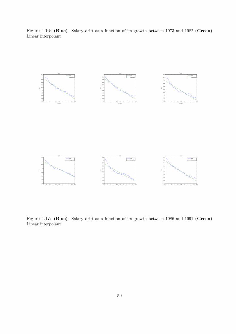
Figure 4.16: (Blue) Salary drift as a function of its growth between 1973 and 1982 (Green)Linear interpolant
0.7 0.8 0.9 1 1.1 1.2 1.3 1.4 1.5 1.6 1.7−0.08
−0.06
−0.04
−0.02
0
0.02
0.04
0.06
0.08
0.1
0.12
Growth
Drift
1986
DriftInterpolator
0.7 0.8 0.9 1 1.1 1.2 1.3 1.4 1.5 1.6 1.7−0.1
−0.08
−0.06
−0.04
−0.02
0
0.02
0.04
0.06
0.08
0.1
Growth
Drift
1987
DriftInterpolator
0.7 0.8 0.9 1 1.1 1.2 1.3 1.4 1.5 1.6 1.7−0.04
−0.02
0
0.02
0.04
0.06
0.08
0.1
0.12
0.14
Growth
Drift
1988
DriftInterpolator
0.7 0.8 0.9 1 1.1 1.2 1.3 1.4 1.5 1.6 1.7−0.2
−0.15
−0.1
−0.05
0
0.05
0.1
0.15
Growth
Drift
1989
DriftInterpolator
0.7 0.8 0.9 1 1.1 1.2 1.3 1.4 1.5 1.6 1.7−0.06
−0.04
−0.02
0
0.02
0.04
0.06
0.08
0.1
0.12
Growth
Drift
1990
DriftInterpolator
0.7 0.8 0.9 1 1.1 1.2 1.3 1.4 1.5 1.6 1.7−0.1
−0.08
−0.06
−0.04
−0.02
0
0.02
0.04
0.06
0.08
Growth
Drift
1991
DriftInterpolator
Figure 4.17: (Blue) Salary drift as a function of its growth between 1986 and 1991 (Green)Linear interpolant
59

0.7 0.8 0.9 1 1.1 1.2 1.3 1.40.1
0.2
0.3
0.4
0.5
0.6
0.7
0.8
0.9
Growth
Vola
tility
1973
VolatilityInterpolator
0.7 0.8 0.9 1 1.1 1.2 1.3 1.40.1
0.2
0.3
0.4
0.5
0.6
0.7
0.8
0.9
Growth
Vola
tility
1974
VolatilityInterpolator
0.7 0.8 0.9 1 1.1 1.2 1.3 1.40.2
0.3
0.4
0.5
0.6
0.7
0.8
0.9
1
Growth
Vola
tility
1976
VolatilityInterpolator
0.7 0.8 0.9 1 1.1 1.2 1.3 1.4 1.5 1.6 1.70.2
0.3
0.4
0.5
0.6
0.7
0.8
0.9
1
Growth
Vola
tility
1985
VolatilityInterpolator
0.7 0.8 0.9 1 1.1 1.2 1.3 1.4 1.5 1.6 1.70.2
0.4
0.6
0.8
1
1.2
1.4
1.6
Growth
Vola
tility
1986
VolatilityInterpolator
0.8 1 1.2 1.4 1.6 1.8 20
0.5
1
1.5
2
2.5
Growth
Vola
tility
1990
VolatilityInterpolator
Figure 4.18: (Blue) Salary volatility as a function of its growth between 1973 and 1990 (Green)Quadratic interpolant
60

0 5 10 15 20 25−14
−13
−12
−11
−10
−9
−8
−7
−6
x 10−4
0 5 10 15 20 25−0.1
−0.08
−0.06
−0.04
−0.02
0
0.02
0.04
0.06
0.08
0.1
Figure 4.19: (Left) Blue The slopes ξ(t) between 1970 and 1992 (Left) Green The average ofξ(t) (Right) Blue The constant terms ξ2(t) between 1970 and 1992 (Right) Black The averageof ξ2(t)
0 5 10 15 20 25
−0.5
0
0.5
1
1.5
0 5 10 15 20 25−40
−30
−20
−10
0
10
20
30
0 5 10 15 20 25−15
−10
−5
0
5
10
15
20
Figure 4.20: (Left) Blue The leading quadratic coefficient, η(t) , between 1970 and 1992 (Left)Green The avefage of η(t) (Middle) Blue The coefficient η2(t) between 1970 and 1992 (Middle)Green The average of η2(t) (Right) Blue The coefficient η3(t) between 1970 and 1992 (Right)Green The average of the constant terms η3(t)
61
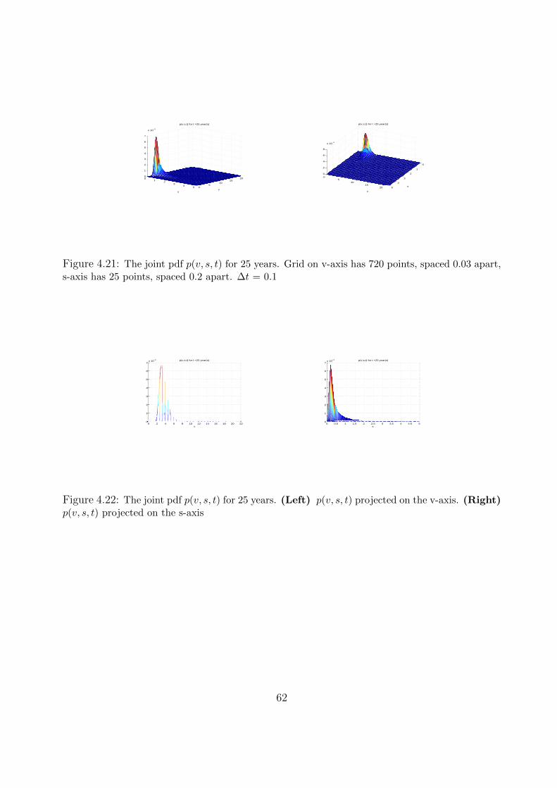
01
23
45 0
510
1520
0
1
2
3
4
5
6
7
x 10−3
v
p(v,s,t) for t =25 year(s)
s
0
1
2
3
4
5
05
1015
20
0
2
4
6
8
x 10−3
s
p(v,s,t) for t =25 year(s)
v
Figure 4.21: The joint pdf p(v, s, t) for 25 years. Grid on v-axis has 720 points, spaced 0.03 apart,s-axis has 25 points, spaced 0.2 apart. ∆t = 0.1
0 2 4 6 8 10 12 14 16 18 20 220
1
2
3
4
5
6
7x 10
−3
v
p(v,s,t) for t =25 year(s)
0 0.5 1 1.5 2 2.5 3 3.5 4 4.5 50
1
2
3
4
5
6
7x 10
−3 p(v,s,t) for t =25 year(s)
s
Figure 4.22: The joint pdf p(v, s, t) for 25 years. (Left) p(v, s, t) projected on the v-axis. (Right)p(v, s, t) projected on the s-axis
62

01
23
45 0
5
10
150
0.5
1
1.5
2
2.5
3
3.5
x 10−3
v
p(v,s,t) for t =50 year(s)
s
0
2
405
1015
0
0.5
1
1.5
2
2.5
3
3.5
x 10−3
s
v
p(v,s,t) for t =50 year(s)
Figure 4.23: The joint pdf p(v, s, t) for 50 years. Grid on v-axis has 720 points, spaced 0.03 apart,s-axis has 25 points, spaced 0.2 apart. ∆t = 0.1
0 2 4 6 8 10 12 14 16 180
0.5
1
1.5
2
2.5
3
3.5x 10
−3
v
p(v,s,t) for t =50 year(s)
0 0.5 1 1.5 2 2.5 3 3.5 4 4.5 50
0.5
1
1.5
2
2.5
3
3.5x 10
−3 p(v,s,t) for t =50 year(s)
s
Figure 4.24: The joint pdf p(v, s, t) for 50 years. (Left) p(v, s, t) projected on the v-axis. (Right)p(v, s, t) projected on the s-axis
63

0 20 40 60 80 100 1200
0.005
0.01
0.015
0.02
0.025
0.03
0.035
age
Distribution of the age of death, US 2003, CDC
Figure 4.25: The pdf of the age of death, US 2003
64

Age Probability of Number Number Person-years Total number Expec.
dying between surviving dying ages lived between of person-years of life
ages x to x+1 to age x between ages ages x to x+1 lived above at age x
x to x+1 age x
0-1 0.006865 100,000 687 99,394 7,743,016 77.4
1-2 0.000469 99,313 47 99,290 7,643,622 77.0
2-3 0.000337 99,267 33 99,250 7,544,332 76.0
3-4 0.000254 99,233 25 99,221 7,445,082 75.0
4-5 0.000194 99,208 19 99,199 7,345,861 74.0
5-6 0.000177 99,189 18 99,180 7,246,663 73.1
6-7 0.000160 99,171 16 99,163 7,147,482 72.1
7-8 0.000147 99,156 15 99,148 7,048,319 71.1
8-9 0.000132 99,141 13 99,134 6,949,171 70.1
9-10 0.000117 99,128 12 99,122 6,850,036 69.1
10-11 0.000109 99,116 11 99,111 6,750,914 68.1
11-12 0.000118 99,105 12 99,100 6,651,803 67.1
12-13 0.000157 99,094 16 99,086 6,552,704 66.1
13-14 0.000233 99,078 23 99,067 6,453,618 65.1
14-15 0.000339 99,055 34 99,038 6,354,551 64.2
15-16 0.000460 99,022 46 98,999 6,255,513 63.2
16-17 0.000577 98,976 57 98,947 6,156,514 62.2
17-18 0.000684 98,919 68 98,885 6,057,566 61.2
18-19 0.000769 98,851 76 98,813 5,958,681 60.3
19-20 0.000832 98,775 82 98,734 5,859,868 59.3
20-21 0.000894 98,693 88 98,649 5,761,134 58.4
21-22 0.000954 98,605 94 98,558 5,662,485 57.4
22-23 0.000990 98,511 98 98,462 5,563,928 56.5
23-24 0.000997 98,413 98 98,364 5,465,466 55.5
24-25 0.000982 98,315 97 98,267 5,367,101 54.6
25-26 0.000960 98,219 94 98,171 5,268,835 53.6
26-27 0.000942 98,124 92 98,078 5,170,663 52.7
27-28 0.000936 98,032 92 97,986 5,072,585 51.7
28-29 0.000947 97,940 93 97,894 4,974,599 50.8
29-30 0.000974 97,847 95 97,800 4,876,705 49.8
30-31 0.001008 97,752 98 97,703 4,778,906 48.9
65

Age Probability of Number Number Person-years Total number Expec.
dying between surviving dying ages lived between of person-years of life
ages x to x+1 to age x between ages ages x to x+1 lived above at age x
x to x+1 age x
31-32 0.001046 97,654 102 97,603 4,681,203 47.9
32-33 0.001097 97,551 107 97,498 4,583,600 47.0
33-34 0.001162 97,444 113 97,388 4,486,102 46.0
34-35 0.001244 97,331 121 97,271 4,388,715 45.1
35-36 0.001336 97,210 130 97,145 4,291,444 44.1
36-37 0.001441 97,080 140 97,010 4,194,299 43.2
37-38 0.001567 96,940 152 96,864 4,097,289 42.3
38-39 0.001714 96,788 166 96,705 4,000,424 41.3
39-40 0.001874 96,623 181 96,532 3,903,719 40.4
40-41 0.002038 96,442 197 96,343 3,807,187 39.5
41-42 0.002207 96,245 212 96,139 3,710,844 38.6
42-43 0.002389 96,033 229 95,918 3,614,705 37.6
43-44 0.002593 95,803 248 95,679 3,518,787 36.7
44-45 0.002819 95,555 269 95,420 3,423,108 35.8
45-46 0.003064 95,285 292 95,139 3,327,688 34.9
46-47 0.003322 94,993 316 94,836 3,232,548 34.0
47-48 0.003589 94,678 340 94,508 3,137,713 33.1
48-49 0.003863 94,338 364 94,156 3,043,205 32.3
49-50 0.004148 93,974 390 93,779 2,949,049 31.4
50-51 0.004458 93,584 417 93,375 2,855,270 30.5
51-52 0.004800 93,167 447 92,943 2,761,895 29.6
52-53 0.005165 92,719 479 92,480 2,668,952 28.8
53-54 0.005554 92,241 512 91,984 2,576,472 27.9
54-55 0.005971 91,728 548 91,454 2,484,487 27.1
55-56 0.006423 91,181 586 90,888 2,393,033 26.2
56-57 0.006925 90,595 627 90,281 2,302,145 25.4
57-58 0.007496 89,968 674 89,630 2,211,864 24.6
58-59 0.008160 89,293 729 88,929 2,122,234 23.8
59-60 0.008927 88,565 791 88,169 2,033,305 23.0
60-61 0.009827 87,774 863 87,343 1,945,136 22.2
61-62 0.010831 86,911 941 86,441 1,857,793 21.4
62-63 0.011872 85,970 1021 85,460 1,771,352 20.6
63-64 0.012891 84,949 1095 84,402 1,685,892 19.8
64-65 0.013908 83,854 1166 83,271 1,601,490 19.1
65-66 0.015003 82,688 1241 82,068 1,518,219 18.4
66-67 0.016267 81,448 1325 80,785 1,436,151 17.6
67-68 0.017699 80,123 1418 79,414 1,355,366 16.9
66
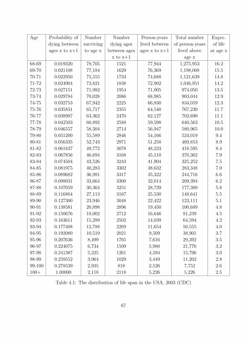
Age Probability of Number Number Person-years Total number Expec.
dying between surviving dying ages lived between of person-years of life
ages x to x+1 to age x between ages ages x to x+1 lived above at age x
x to x+1 age x
68-69 0.019320 78,705 1521 77,944 1,275,953 16.2
69-70 0.021108 77,184 1629 76,369 1,198,008 15.5
70-71 0.022950 75,555 1734 74,688 1,121,639 14.8
71-72 0.024904 73,821 1838 72,902 1,046,951 14.2
72-73 0.027151 71,982 1954 71,005 974,050 13.5
73-74 0.029784 70,028 2086 68,985 903,044 12.9
74-75 0.032753 67,942 2225 66,830 834,059 12.3
75-76 0.035831 65,717 2355 64,540 767,230 11.7
76-77 0.038987 63,362 2470 62,127 702,690 11.1
77-78 0.042503 60,892 2588 59,598 640,563 10.5
78-79 0.046557 58,304 2714 56,947 580,965 10.0
79-80 0.051200 55,589 2846 54,166 524,019 9.4
80-81 0.056335 52,743 2971 51,258 469,853 8.9
81-82 0.061837 49,772 3078 48,233 418,595 8.4
82-83 0.067856 46,694 3168 45,110 370,362 7.9
83-84 0.074504 43,526 3243 41,904 325,252 7.5
84-85 0.081975 40,283 3302 38,632 283,348 7.0
85-86 0.089682 36,981 3317 35,322 244,716 6.6
86-87 0.098031 33,664 3300 32,014 209,394 6.2
87-88 0.107059 30,364 3251 28,739 177,380 5.8
88-89 0.116804 27,113 3167 25,530 148,641 5.5
89-90 0.127300 23,946 3048 22,422 123,111 5.1
90-91 0.138581 20,898 2896 19,450 100,689 4.8
91-92 0.150676 18,002 2712 16,646 81,239 4.5
92-93 0.163611 15,289 2502 14,039 64,594 4.2
93-94 0.177408 12,788 2269 11,654 50,555 4.0
94-95 0.192080 10,519 2021 9,509 38,901 3.7
95-96 0.207636 8,499 1765 7,616 29,392 3.5
96-97 0.224075 6,734 1509 5,980 21,776 3.2
97-98 0.241387 5,225 1261 4,594 15,796 3.0
98-99 0.259552 3,964 1029 3,449 11,202 2.8
99-100 0.278539 2,935 818 2,526 7,752 2.6
100+ 1.00000 2,118 2118 5,226 5,226 2.5
Table 4.1: The distribution of life span in the USA, 2003 (CDC)
67

Bibliography
[1] Gerstenhaber, M. Have You Ever Seen A Retired Tiger In The Jungle, Retired TigersPublications, Switzerland 2009
[2] Clark, R.L., L.A. Craig, J.W. Wilson. A History of Public Sector Pensions in the UnitedStates., University of Pennsylvania Press, Philadelphia, PA 2003
[3] McDonnell, K., B.B. Burr History of Pension Plans, U.S Government Printing Office,EBRI Databook on Employee Benefits fourth edition, Washington, DC 1997
[4] Corbett, T. Local Government Law Library , Pennsylvania Department Community &Economic Development, 2011
[5] Keegan, B. The Trillion Dollar Gap, The PEW charitable trusts., Public SectorRetirement Systems, The Widening Gap, http://www.pewstates.org/research/data-visualizations/the-widening-gap-85899377237 , 2012
[6] ”Old Age, Survivors And Disability Insurance Program (OASDI), Trustees Re-port” The United States Social Security Administration, Office of the Chief Actuaryhttp://www.ssa.gov/OACT/TR/2013/tr2013.pdf (2010)
[7] Russek, F. The Underfunding of State and Local Pension Plans, Congressional BudgetOffice United States Government www.cbo.gov/sites/default/files/cbofiles/ ftpdocs/120xx/doc12084/05-04-pensions.pdf, , Washington, D.C. 2011
[8] Coggan, P. Falling Short, The Economist, http://www.economist.com/node/18502013 ,Apr 9th, 2011
[9] Monetary and Capital Markets Department, International Monetary Fund Global Fi-nancial Stability Report , http://www.imf.org/external/pubs/ft/gfsr/index.htm , 2012
[10] Browning, E.S., ”Exorcising Ghosts of Octobers Past,” The Wall Street Journal , pp.C1C2. (2007-10-15)
[11] Gramling W.R., Financial Audit - Resolution Trust Corporation’s 1995 and 1994 Fi-nancial Statements , United States General Accounting Office, Washington, D.C. 1996
[12] Feridun, M., ”Russian Financial Crisis of 1998: An Economic Investigation,”, Interna-tional Journal of Applied Econometrics and Quantitative Studies, 1-4 (2004)
68

[13] Greenspan, Alan. The Age of Turbulence: Adventures in a New World, pp. 193-195,The Penguin Press, London, UK 2007
[14] Federal Reserve Bank of St. Louis, Federal Reserve Economic Datahttp://research.stlouisfed.org/fred2/
[15] Phillips, M. Nasdaq: Heres Our Timeline of the Flash Crash, Wall Street Journal, May11. 2010
[16] Valetkevitch, C., C. Mikolajczak Error by Knight Capital rips through stock market,Reuters, Aug 1. 2012
[17] S&P Dow Jones Indices, McGraw Hill Financial S& P U.S Indices Methoodlogy 2013.
[18] Fama, E.F., ”Efficient Capital Markets,” The Journal of Finance, 46(5) (1991)
[19] Center for Research in Security Prices CRSP/COMPUSTAT Merged Database TheUniversity of Chicago, Booth School of Business.
[20] von Mises, L. ”Economic Calculation In The Socialist Commonwealth”, Archiv furSozialwissenschaften 47 (1920)
[21] Bellamy, R. The Cambridge History of Twentieth-Century Political Thought, pp.60,Cambridge University Press, Cambridge, UK 2003
[22] Riedl, M.B. Why Governments Spending Does Not Stimulate Economic Growt: An-swering the Critics, Wall Street Journal Jan 8. 2010
[23] Utt, R.D., ”More Transportation Spending: Fales Promises of Prosperity and Job Cre-ation,” The Heritage Foundation, 2121 (2008)
[24] Baily N. M. , K. Croxson , T. Dohrmann , L. Mendonca The public-sector productivityimperative. McKinsey & Company 2011
[25] Haskel J., Wallis G. ”Public support for innovation, intangible investment and produc-tivity growth in the UK market sector,” IZA 4772 (2010)
[26] Cont, R., P. Tankov, Financial Modelling With Jump Processes, Chapman & Hall,Financial Mathematics, London, UK 2009
[27] Heston, L. S. , ”A Closed-Form Solution for Options with Stochastic Volatility withApplications to Bond and Currency Options,” The Review of Financial Studies 6 (2)pp.327–343 (1993)
[28] Hagan S. P., K. Deep, S.A. Lesniewski, D.E. Woodward, ”Managing Smile Risk” ,WILLMOTT Magazine, http://www.wilmott.com/pdfs/021118 smile.pdf (2002)
[29] Chen, L. , ”Stochastic Mean and Stochastic Volatility A Three-Factor Model of theTerm Structure of Interest Rates and Its Application to the Pricing of Interest RateDerivatives”, Financial Markets, Institutions, and Instruments, 5 (1-88) (1996)
69

[30] Schuss, Z., Diffusion and Stochastic Processes: an Analytical Approach, Springer, Ap-plied Mathematical Sciences 170, NY,NY (2010)
[31] Senaratne D., Chintha T., ”Numerical computation of the lognormal sum distribution,”Global Telecommunications Conference, IEEE pp.1–6 (2009)
[32] Cobb R. B., A. Salmeron, R. Rumi, ”Approximating the Distribution of a Sum of aLog-normal Random Variables,” Statistics and Computing 16(3), pp. 293-308 (2012)
[33] Dufresne, D., ”The log-normal approximation in financial and other applications,” Adv.Applied Probability, 36 , pp.747–773 (2004)
[34] Skorokhod, A.V ”Stochastic equations for diffusion processes in a bounded region,”Theor: Probab. Appl., 6(3), pp.264–275 (1961)
[35] Panel Study of Income Dynamics, public use dataset. Survey Research Center, Institutefor Social Research, University of Michigan, Ann Arbor, MI (2013).
[36] Crank, J., The Mathematics of Diffusion, pp. 137–160, Oxford University Press, Ox-ford, UK, 1975
[37] Cohen, B. S., I. N. Kirschner ”Approximating the Dirac Distribution for Fourier Anal-ysis,” Journal of Computational Physics 93 pp.314-315 (1991)
[38] Zelen, M., Norman C. Severo Handbook of mathematical functions with formulas,graphs, and mathematical tables, Dover Pulications, Mineola, NY (1964)
[39] Hart, John F. Computer Approximations, John Wiley & Sons, NY, NY. (1968)
[40] Cody, William J., ”Rational Chebyshev Approximations for the Error Function,” Math-ematics of Computation, 23 (107) (1969)
[41] Saad Y., M.H. Schultzm ”GMRES: A generalized minimal residual algorithm for solvingnonsymmetric linear systems,” SIAM J. Sci. Stat. Comput., 7, pp.856–869 (1986)
[42] Arnoldi, W. E., ”The principle of minimized iterations in the solution of the matrixeigenvalue problem,” Quarterly of Applied Mathematics, 9, pp.17-29 (1951)
[43] Van Loan, C.F, Gene H. Golub Matrix Computations, JHU Press, Baltimore, MD(1996)
[44] Arias, E. ”United States Life Tables, 2003,” Center for Disease Control and Prevention,National Vital Statistics Reports, NVSS, 54(14) (2003)
[45] Coifman, R.R. ”Preface,” Have You Ever Seen A Retired Tiger In The Jugnle, pp.8–9(2009)
70