Stochastic Methods for ℓ1-regularized Loss Minimization ...jmlr.org/papers/volume12/shalev-shwartz11a/shalev-shwartz11a.pdf · convex optimization problem, and therefore can be

Journal of Machine Learning Research 12 (2011) 1865-1892 Submitted 12/10; Revised 5/11; Published 6/11

Stochastic Methods forℓ1-regularized Loss Minimization

Shai Shalev-Shwartz [email protected] of Computer Science and EngineeringThe Hebrew University of JerusalemGivat Ram, Jerusalem 91904, Israel

Ambuj Tewari [email protected]

Computer Science DepartmentThe University of Texas at AustinAustin, TX 78701, USA

Editor: Leon Bottou

AbstractWe describe and analyze two stochastic methods forℓ1 regularized loss minimization problems,such as the Lasso. The first method updates the weight of a single feature at each iteration whilethe second method updates the entire weight vector but only uses a single training example ateach iteration. In both methods, the choice of feature or example is uniformly at random. Ourtheoretical runtime analysis suggests that the stochasticmethods should outperform state-of-the-artdeterministic approaches, including their deterministiccounterparts, when the size of the problemis large. We demonstrate the advantage of stochastic methods by experimenting with synthetic andnatural data sets.1

Keywords: L1 regularization, optimization, coordinate descent, mirror descent, sparsity

1. Introduction

We present optimization procedures for solving problems of the form:

minw∈Rd

1m

m

∑i=1

L(〈w,xi〉,yi)+λ‖w‖1 , (1)

where(x1,y1), . . . ,(xm,ym) ∈ ([−1,+1]d×Y )m is a sequence of training examples,L : Rd×Y →[0,∞) is a non-negative loss function, andλ > 0 is a regularization parameter. This generic problemincludes as special cases the Lasso (Tibshirani, 1996), in whichL(a,y) = 1

2(a− y)2, and logisticregression, in whichL(a,y) = log(1+exp(−ya)).

Our methods can also be adapted to deal with additional boxed constraints ofthe formwi ∈[ai ,bi ], which enables us to use them for solving the dual problem of Support Vector Machine(Cristianini and Shawe-Taylor, 2000). For concreteness, we focuson the formulation given in (1).

Throughout the paper, we assume thatL is convex in its first argument. This implies that (1) is aconvex optimization problem, and therefore can be solved using standard optimization techniques,such as interior point methods. However, standard methods scale poorly with the size of the problem(i.e., m andd). In recent years, machine learning methods are proliferating in data-laden domainssuch as text and web processing in which data sets of millions of training examples or features are

1. An initial version of this work (Shalev-Shwartz and Tewari, 2009) appeared in ICML 2009.

c©2011 Shai Shalev-Shwartz and Ambuj Tewari.

SHALEV-SHWARTZ AND TEWARI

not uncommon. Since traditional methods for solving (1) generally scale very poorly with the sizeof the problem, their usage is inappropriate for data-laden domains. In this paper, we discuss how toovercome this difficulty using stochastic methods. We describe and analyze two practical methodsfor solving (1) even when the size of the problem is very large.

The first method we propose is a stochastic version of the familiar coordinatedescent approach.The coordinate descent approach for solvingℓ1 regularized problems is not new (as we survey belowin Section 1.1). At each iteration of coordinate descent, a single element ofw is updated. The onlytwist we propose here regarding the way one should choose the next feature to update. We suggestto choose features uniformly at random from the set[d] = 1, . . . ,d. This simple modificationenables us to show that the runtime required to achieveε (expected) accuracy is upper bounded by

mdβ‖w⋆‖22ε

, (2)

whereβ is a constant which only depends on the loss function (e.g.,β = 1 for the quadratic lossfunction) andw⋆ is the optimal solution. This bound tells us that the runtime grows only linearlywith the size of the problem. Furthermore, the stochastic method we propose is parameter free andvery simple to implement.

Another well known stochastic method that has been successfully applied for loss minimizationproblems, is stochastic gradient descent (e.g., Bottou and LeCunn, 2005; Shalev-Shwartz et al.,2007). In stochastic gradient descent, at each iteration, we pick one example from the training set,uniformly at random, and update the weight vector based on the chosen example. The attractivenessof stochastic gradient descent methods is that their runtime do not depend at all on the number ofexamples, and can even sometime decrease with the number of examples (see Bottou and Bousquet,2008; Shalev-Shwartz and Srebro, 2008). Unfortunately, the stochastic gradient descent methodfails to produce sparse solutions, which makes the algorithm both slower andless attractive assparsity is one of the major reasons to useℓ1 regularization. To overcome this problem, two variantswere recently proposed. First, Duchi et al. (2008) suggested to replace theℓ1 regularization termwith a constraint of the form‖w‖1 ≤ B, and then to use stochastic gradient projection procedure.Another solution, which uses the regularization form given in (1), has been proposed by Langfordet al. (2009) and is called truncated gradient descent. In this approach, the elements ofw that cross0 after the stochastic gradient step are truncated to 0, hence sparsity is achieved. The disadvantageof both Duchi et al. (2008) and Langford et al. (2009) methods is that, insome situations, theirruntime might grow quadratically with the dimensiond, even if the optimal predictorw⋆ is verysparse (see Section 1.1 below for details). This quadratic dependence on d can be avoided if oneuses mirror descent updates (Beck and Teboulle, 2003) such as the exponentiated gradient approach(Littlestone, 1988; Kivinen and Warmuth, 1997; Beck and Teboulle, 2003). However, this approachagain fails to produce sparse solutions. In this paper, we combine the idea of truncating the gradient(Langford et al., 2009) with another variant of stochastic mirror descent, which is based onp-normupdates (Grove et al., 2001; Gentile, 2003). The resulting algorithm both produces sparse solutionsand hasO(d) dependence on the dimension. We call the algorithm SMIDAS for “StochasticMIrrorDescent Algorithm made Sparse”.

We provide runtime guarantees for SMIDAS as well. In particular, for the logistic-loss and thesquared-loss we obtain the following upper bound on the runtime to achievingε expected accuracy:

O

(d log(d)‖w⋆‖21

ε2

)

. (3)

1866

STOCHASTIC METHODS FORℓ1-REGULARIZED LOSSM INIMIZATION

Comparing the above with the runtime bound of the stochastic coordinate descent method givenin (2) we note three major differences. First, while the bound in (2) depends on the number ofexamples,m, the runtime of SMIDAS does not depend onmat all. On the flip side, the dependenceof stochastic coordinate descent on the dimension is better both because thelack of the term log(d)and because‖w⋆‖22 is always smaller than‖w⋆‖21 (the ratio is at mostd). Last, the dependence on1

εis linear in (2) and quadratic in (3). Ifε is the same order as the objective value atw⋆, it is possibleto improve the dependence on 1/ε (Proposition 4). Finally, we would like to point out that while thestochastic coordinate descent method is parameter free, the success of SMIDAS and of the methodof Langford et al. (2009), depends on a careful tuning of a learningrate parameter.

1.1 Related Work

We now survey several existing methods and in particular show how our stochastic twist enables usto give superior runtime guarantees.

1.1.1 COORDINATE DESCENTMETHODSFOR ℓ1 REGULARIZATION

Following the Gauss-Siedel approach of Zhang and Oles (2001), Genkin et al. (2007) described acoordinate descent method (called BBR) for minimizingℓ1 regularized objectives. This approach issimilar to our method, with three main differences. First, and most important, at each iteration wechoose a coordinate uniformly at random. This allows us to provide theoretical runtime guarantees.We note that no theoretical guarantees are provided by Zhang and Oles (2001) and Genkin et al.(2007). Second, we solely use gradient information which makes our algorithm parameters-freeand extremely simple to implement. In contrast, the Gauss-Siedel approach is more complicatedand involves second order information, or a line search procedure, ora trusted region Newton step.Last, the generality of our derivation allows us to tackle a more general problem. For example, itis easy to deal with additional boxed constraints. Friedman et al. (2010) generalized the approachof Genkin et al. (2007) to include the case of elastic-net regularization. In a series of experiments,they observed that cyclic coordinate descent outperforms many alternative popular methods suchas LARS (Efron et al., 2004), an interior point method calledl1lognet (Koh et al., 2007), and theLasso Penalized Logistic (LPL) program (Wu and Lange, 2008). However, no theoretical guaranteesare provided in Friedman et al. (2010) as well. Our analysis can partially explain the experimentalresult of Friedman et al. (2010) since updating the coordinates in a cyclic order can in practice bevery similar to stochastic updates.

Luo and Tseng (1992) established a linear convergence result for coordinate descent algorithms.This convergence result tells us that after an unspecified number of iterations, the algorithm con-verges very fast to the optimal solution. However, this analysis is useless indata laden domains asit can be shown that the initial unspecified number of iterations depends at least quadratically on thenumber of training examples. In an attempt to improve the dependence on the size of the problem,Tseng and Yun (2009) recently studied other variants of block coordinate descent for optimizing‘smooth plus separable’ objectives. In particular,ℓ1 regularized loss minimization (1) is of thisform, provided that the loss function is smooth. The algorithm proposed by Tseng and Yun (2009)is not stochastic. Translated to our notation, the runtime bound given in Tseng and Yun (2009) is

1867


of order2 md2 β‖w⋆‖22ε . This bound is inferior to our runtime bound for stochastic coordinate descent

given in (2) by a factor of the dimensiond.

1.1.2 COORDINATE DESCENTMETHODSFOR ℓ1 DOMAIN CONSTRAINTS

A different, but related, optimization problem is to minimize the loss,1m ∑i L(〈w,xi〉,yi), subject

to a domain constraint of the form‖w‖1 ≤ B. Many authors presented a forward greedy selectionalgorithm (a.k.a. Boosting) for this problem. We refer the reader to Frank and Wolfe (1956), Zhang(2003), Clarkson (2008) and Shalev-Shwartz et al. (2010). Theseauthors derived the upper boundO(β‖w⋆‖21/ε

)on the number of iterations required by this algorithm to find anε-accurate solution.

Since at each iteration of the algorithm, one needs to calculate the gradient ofthe loss atw, theruntime of each iteration ismd. Therefore, the total runtime becomesO

(mdβ‖w⋆‖21/ε

). Note

that this bound is better than the bound given by Tseng and Yun (2009), since for any vector inRd

we have‖w‖1 ≤√

d‖w‖2. However, the boosting bound given above is still inferior to our boundgiven in (2) since‖w⋆‖1≥ ‖w⋆‖2. Furthermore, in the extreme case we have‖w⋆‖21 = d‖w⋆‖22, thusour bound can be better than the boosting bound by a factor ofd. Lemma 5 in Appendix A showsthat theiteration bound (not runtime) ofany algorithm cannot be smaller thanΩ(‖w⋆‖21/ε) (seealso the lower bounds in Shalev-Shwartz et al., 2010). This seems to imply thatanydeterministicmethod, which goes over the entire data at each iteration, will induce a runtime which is inferior tothe runtime we derive for stochastic coordinate descent.

1.1.3 STOCHASTIC GRADIENT DESCENT ANDM IRROR DESCENT

Stochastic gradient descent (SGD) is considered to be one of the best methods for large scale lossminimization, when we measure how fast a method achieves a certain generalization error. Thishas been observed in experiments (Bottou, Web Page) and also has beenanalyzed theoretically byBottou and Bousquet (2008) and Shalev-Shwartz and Srebro (2008).

As mentioned before, one can apply SGD for solving (1). However, SGDfails to produce sparsesolutions. Langford et al. (2009) proposed an elegant simple modificationof the SGD update rulethat yields a variant of SGD with sparse intermediate solutions. They also provide bounds on theruntime of the resulting algorithm. In the general case (i.e., without assuming lowobjective relativeto ε), their analysis implies the following runtime bound

O

(d‖w⋆‖22X2

2

ε2

)

, (4)

whereX22 = 1

m ∑i ‖xi‖22 is the average squared norm of an instance. Comparing this bound with ourbound in (3), we observe that none of the bounds dominates the other, and their relative performancedepends on properties of the training set and the optimal solutionw⋆. Specifically, ifw⋆ has onlyk≪ d non-zero elements and eachxi is dense (sayxi ∈ −1,+1d), then the ratio between theabove bound of SGD and the bound in (3) becomesdk log(d) ≫ 1. On the other hand, ifxi has only

k non-zeros whilew⋆ is dense, then the ratio between the bounds can bekd log(d) ≪ 1. Although the

relative performance is data dependent, in most applications if one prefers ℓ1 regularization overℓ2

2. To see this, note that the iterations bound in Equation (21) of Tseng and Yun (2009) is:β‖w⋆‖22

εν , and using Equation(25) in Section 6, we can set the value ofν to beν = 1/d (since in our case there are no linear constraints). Thecomplexity bound now follows from the fact that the cost of each iteration isO(d m).

1868


regularization, he should also believe thatw⋆ is sparse, and thus our runtime bound in (3) is likelyto be superior.3

The reader familiar with the online learning and mirror descent literature will not be surprisedby the above discussion. Bounds that involved‖w⋆‖1 and‖xi‖∞, as in (3), are well known and therelative performance discussed above was pointed out in the context ofadditive vs. multiplicativeupdates (see, e.g., Kivinen and Warmuth, 1997). However, the most popular algorithm for obtainingbounds of the form given in (3) is the EG approach (Kivinen and Warmuth, 1997), which involvesthe exponential potential, and this algorithm cannot yield intermediate sparse solutions. One of thecontributions of this paper is to show that with a different potential, which is called the p-normpotential, one can obtain the bound given in (3) while still enjoying sparse intermediate solutions.

1.1.4 RECENT WORKS DEALING WITH STOCHASTIC METHODS FORLARGE SCALE

REGULARIZED LOSSM INIMIZATION

Since the publication of the conference version (Shalev-Shwartz and Tewari, 2009) of this paper,several papers proposing stochastic algorithms for regularized loss minimization have appeared. Ofthese, we would like to mention a few that are especially connected to the themes pursued in thepresent paper. Regularized Dual Averaging (RDA) of Xiao (2010) uses a running average of allthe past subgradients of the loss function and the regularization term to generate its iterates. Hedevelops ap-norm RDA method that is closely related to SMIDAS. The theoretical boundsforSMIDAS andp-norm RDA are similar but the latter employs a more aggressive truncation schedulethat can potentially lead to sparser iterates.

SMIDAS deals withℓ1 regularization. The Composite Objective MIrror Descent (COMID) al-gorithm of Duchi et al. (2010) generalizes the idea behind SMIDAS to deal with general regularizersprovided a certain minimization problem involving a Bregman divergence and the regularizer is ef-ficiently solvable. Viewing the average loss in (1) leads to interesting connections with the areaof Stochastic Convex Optimization that deals with minimizing a convex function given access toan oracle that can return unbiased estimates of the gradient of the convexfunction at any querypoint. For various classes of convex functions, one can ask: What is the optimal number of queriesneeded to achieve a certain accuracy (in expectation)? For developmentsalong these lines, pleasesee Lan (2010) and Ghadimi and Lan (2011), especially the latter since it deals with functions thatare the sum of a smooth and a non-smooth but “simple” (likeℓ1-norm) part. Finally, Nesterov(2010) has analyzed randomized versions of coordinate descent forunconstrained and constrainedminimization of smooth convex functions.

2. Stochastic Coordinate Descent

To simplify the notation throughout this section, we rewrite the problem in (1) using the notation

minw∈Rd

≡P(w)︷︸︸︷

1m

m

∑i=1

L(〈w,xi〉,yi)

︸︷︷︸

≡C(w)

+λ‖w‖1 . (5)

3. One important exception is the large scale text processing application described in Langford et al. (2009) where thedimension is so large andℓ1 is used simply because we cannot store a dense weight vector in memory.

1869


We are now ready to present the stochastic coordinate descent algorithm.The algorithm ini-tializesw to be0. At each iteration, we pick a coordinatej uniformly at random from[d]. Then,the derivative ofC(w) w.r.t. the jth element ofw, g j = (∇C(w)) j , is calculated. That is,g j =1m ∑m

i=1L′(〈w,xi〉,yi)xi, j , whereL′ is the derivative of the loss function with respect to its first argu-ment. Simple calculus yields

L′(a,y) =

(a−y) for squared-loss−y

1+exp(ay) for logistic-loss. (6)

Next, a step size is determined based on the value ofg j and a parameter of the loss function denotedby β. This parameter is an upper bound on the second derivative of the loss.Again, for our runningexamples we have

β =

1 for squared-loss

1/4 for logistic-loss. (7)

If there was no regularization, we would just subtract the step sizeg j/β from the current value ofw j . However, to take into account the regularization term, we further add/subtract λ/β from w j

provided we do not cross 0 in the process. If we do, we let the new valueof w j be exactly 0. Thisis crucial for maintaining sparsity ofw. To describe the entire update succinctly, it is convenient todefine the following simple “thresholding” operation:

sτ(w) = sign(w)(|w|− τ)+ =

0 w∈ [−τ,τ]w− τ w> τw+ τ w<−τ

.

Algorithm 1 Stochastic Coordinate Descent (SCD)let w = 0for t = 1,2, . . . do

samplej uniformly at random from1, . . . ,dlet g j = (∇C(w)) j

w j ← sλ/β(w j −g j/β)end for

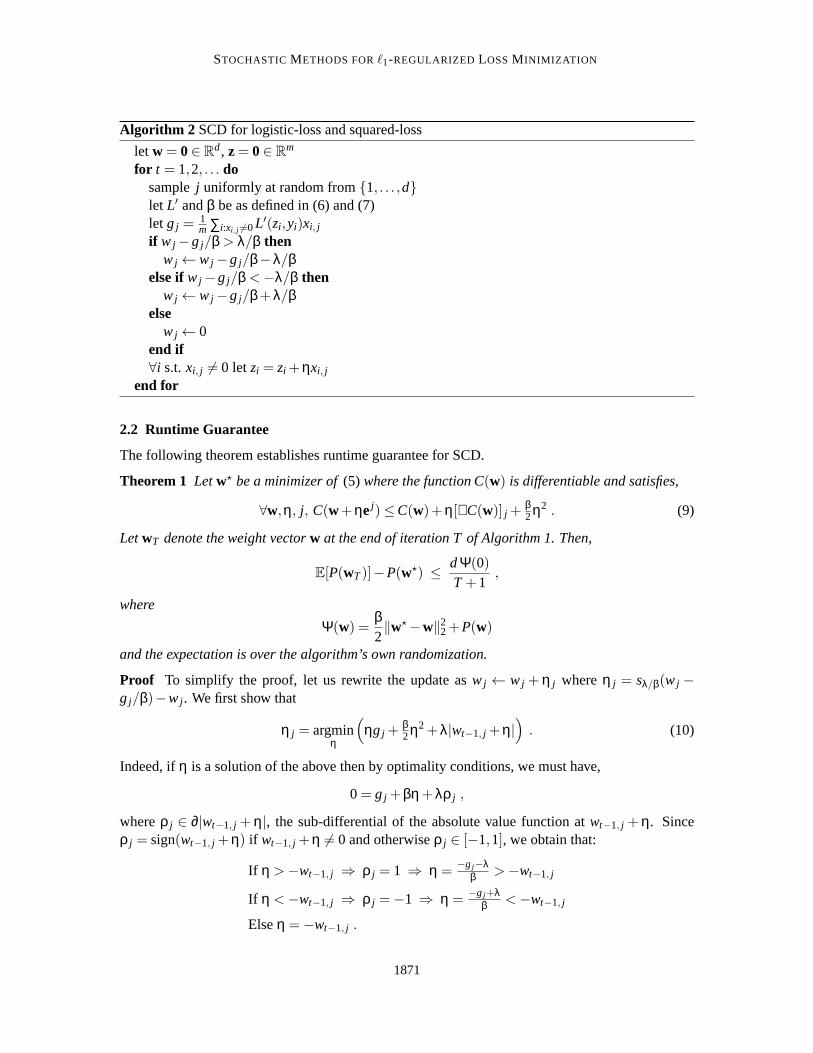
2.1 Efficient Implementation

We now present an efficient implementation of Algorithm 1. The simple idea is to maintain a vectorz∈ R

m such thatzi = 〈w,xi〉. Once we have this vector, calculatingg j on average requiresO(sm)iterations, where

s= |(i, j) : xi, j 6=0|md (8)

is the average number of non-zeros in our training set. Concretely, we obtain Algorithm 2 forlogistic-loss and squared-loss.

1870


Algorithm 2 SCD for logistic-loss and squared-loss

let w = 0∈ Rd, z= 0∈ R

m

for t = 1,2, . . . dosamplej uniformly at random from1, . . . ,dlet L′ andβ be as defined in (6) and (7)let g j =

1m ∑i:xi, j 6=0L′(zi ,yi)xi, j

if w j −g j/β > λ/β thenw j ← w j −g j/β−λ/β

else ifw j −g j/β <−λ/β thenw j ← w j −g j/β+λ/β

elsew j ← 0

end if∀i s.t. xi, j 6= 0 letzi = zi +ηxi, j

end for

2.2 Runtime Guarantee

The following theorem establishes runtime guarantee for SCD.

Theorem 1 Letw⋆ be a minimizer of(5) where the function C(w) is differentiable and satisfies,

∀w,η, j, C(w+ηej)≤C(w)+η[∇C(w)] j +β2η2 . (9)

LetwT denote the weight vectorw at the end of iteration T of Algorithm 1. Then,

E[P(wT)]−P(w⋆) ≤ dΨ(0)T +1

,

where

Ψ(w) =β2‖w⋆−w‖22+P(w)

and the expectation is over the algorithm’s own randomization.

Proof To simplify the proof, let us rewrite the update asw j ← w j + η j whereη j = sλ/β(w j −g j/β)−w j . We first show that

η j = argminη

(

ηg j +β2η2+λ|wt−1, j +η|

)

. (10)

Indeed, ifη is a solution of the above then by optimality conditions, we must have,

0= g j +βη+λρ j ,

whereρ j ∈ ∂|wt−1, j +η|, the sub-differential of the absolute value function atwt−1, j +η. Sinceρ j = sign(wt−1, j +η) if wt−1, j +η 6= 0 and otherwiseρ j ∈ [−1,1], we obtain that:

If η >−wt−1, j ⇒ ρ j = 1 ⇒ η =−g j−λ

β >−wt−1, j

If η <−wt−1, j ⇒ ρ j =−1 ⇒ η =−g j+λ

β <−wt−1, j

Elseη =−wt−1, j .

1871


But, this is equivalent to the definition ofη j and therefore (10) holds.Define the potential,

Φ(wt) =12‖w

⋆−wt‖22 ,

and let∆t, j = Φ(wt−1)−Φ(wt−1+η jej) be the change in the potential assuming we updatewt−1

using coordinatej. Since 0= g j +βη j +λρ j , we have that,

∆t, j =12‖w

⋆−wt−1‖22− 12‖w

⋆−wt−1−η jej‖22= 1

2(w⋆j −wt−1, j)

2− 12(w

⋆j −wt−1, j −η j)

2

= 12η2

j −η j(wt−1, j +η j −w⋆j )

= 12η2

j +g j

β(wt−1, j +η j −w⋆

j )+λρ j

β(wt−1, j +η j −w⋆

j ).

Next, we note that

ρ j(wt−1, j +η j −w⋆j )≥ |wt−1, j +η j |− |w⋆

j | ,

which yields

∆t, j ≥ 12η2

j +g j

β(wt−1, j +η j −w⋆

j )+λβ(|wt−1, j +η j |− |w⋆

j |) .

By (9), we have,

C(wt−1+η jej)−C(wt−1)≤ g jη j +β2

η2j ,

and thus

∆t, j ≥1β(C(wt−1+η jej)−C(wt−1))+

g j

β(wt−1, j −w⋆

j )+λβ(|wt−1, j +η j |− |w⋆

j |) .

Taking expectations (with respect to the choice ofj and conditional onwt−1) on both sides, we get,

E[Φ(wt−1)−Φ(wt) |wt−1] =1d

d

∑k=1

∆t,k

≥ 1βd

[d

∑k=1

(C(wt−1+ηkek)−C(wt−1))+d

∑k=1

gk(wt−1,k−w⋆k)+λ

d

∑k=1

(|wt−1,k+ηk|− |w⋆k|)]

=1

βd

[d

∑k=1

(C(wt−1+ηkek)−C(wt−1))+ 〈∇C(wt−1),wt−1−w⋆)〉+λd

∑k=1

(|wt−1,k+ηk|− |w⋆k|)]

≥ 1βd

[d

∑k=1

(C(wt−1+ηkek)−C(wt−1))+C(wt−1)−C(w⋆)+λd

∑k=1

(|wt−1,k+ηk|− |w⋆k|)]

=1β

[

E[C(wt) |wt−1]−C(wt−1)+C(wt−1)−C(w⋆)

d+

λd

d

∑k=1

|wt−1,k+ηk|−λ‖w⋆‖1

d

]

,

1872


where the second inequality follows from the convexity ofC. Note that, we have,

E[‖wt‖1 |wt−1] =1d

d

∑k=1

‖wt−1+ηkek‖1

=1d

d

∑k=1

(‖wt−1‖1−|wt−1,k|+ |wt−1,k+ηk|)

= ‖wt−1‖1−1d‖wt−1‖1+

1d

d

∑k=1

|wt−1,k+ηk| .

Plugging this above gives us,

βE[Φ(wt−1)−Φ(wt) |wt−1]

≥ E[C(wt)+λ‖wt‖1 |wt−1]−C(wt−1)−λ‖wt−1‖1+C(wt−1)+λ‖wt−1‖1−C(w⋆)−λ‖w⋆‖1

d

= E[P(wt) |wt−1]−P(wt−1)+P(wt−1)−P(w⋆)

d.

This is equivalent to,

E[βΦ(wt−1)+P(wt−1)−βΦ(wt)−P(wt) |wt−1]≥P(wt−1)−P(w⋆)

d.

Thus, defining the composite potential,

Ψ(w) = βΦ(w)+P(w) ,

and taking full expectations, we get,

E[Ψ(wt−1)−Ψ(wt)]≥1dE[P(wt−1)−P(w⋆)] .

Summing overt = 1, . . . ,T +1 and realizing thatP(wt) monotonically decreases gives,

E[

T+1d (P(wT)−P(w⋆))

]≤ E

[

1d

T+1

∑t=1

(P(wt−1)−P(w⋆))

]

≤ E

[T+1

∑t=1

(Ψ(wt−1)−Ψ(wt))

]

= E [Ψ(w0)−Ψ(wT+1)] ≤ E [Ψ(w0)] = Ψ(0) .

The above theorem bounds the expected performance of SCD. We nextgive bounds that holdwith high probability.

Theorem 2 Assume that the conditions of Theorem 1 holds. Then, with probability of atleast1/2we have that

P(wT)−P(w⋆) ≤ 2dΨ(0)T +1

.

1873


Furthermore, for anyδ∈ (0,1), suppose we run SCD r= ⌈log2(1/δ)⌉ times, each time T iterations,and letw be the best solution out of the r obtained solutions, then with probability of at least1−δ,

P(w)−P(w⋆) ≤ 2dΨ(0)T +1

.

Proof The random variableP(wT)−P(w⋆) is non-negative and therefore the first inequality followsfrom Markov’s inequality using Theorem 1. To prove the second result,note that the probabilitythat on allr rounds it holds thatP(wT)−P(w⋆) > 2dΨ(0)

T+1 is at most 2−r ≤ δ, which concludes ourproof.

Next, we specify the runtime bound for the case ofℓ1 regularized logistic-regression and squared-loss. First, Lemma 6 in Appendix B shows that forC as defined in (5), if the second derivative ofLis bounded byβ then the condition onC given in Theorem 1 holds. Additionally, for the logistic-losswe haveC(0)≤ 1. Therefore, for logistic-loss, after performing

d(14 ‖w⋆‖22+2)

ε

iterations of Algorithm 2 we achieve (expected)ε-accuracy in the objectiveP. Since the averagecost of each iteration issm, wheres is as defined in (8), we end up with the total runtime

smd(14 ‖w⋆‖22+2)

ε.

The above is the runtime required to achieve expectedε-accuracy. Using Theorem 2 the requiredruntime to achieveε-accuracy with a probability of at least 1−δ is

smd

(

(12 ‖w⋆‖22+4)

ε+ ⌈log(1/δ)⌉

)

.

For the squared-loss we haveC(0) = 1m ∑i y

2i . Assuming that the targets are normalized so that

C(0)≤ 1, and using similar derivation we obtain the total runtime bound

smd

((2‖w⋆‖22+4)

ε+ ⌈log(1/δ)⌉

)

.

3. Stochastic Mirror Descent Made Sparse

In this section, we describe our mirror descent approach forℓ1 regularized loss minimization thatmaintains intermediate sparse solutions. Recall that we rewrite the problem in (1) using the notation

minw∈Rd

≡P(w)︷︸︸︷

1m

m

∑i=1

L(〈w,xi〉,yi)

︸︷︷︸

≡C(w)

+λ‖w‖1 . (11)

1874


Mirror descent algorithms (Nemirovski and Yudin, 1978, Chapter 3) maintain two weight vec-tors: primalw and dualθ. The connection between the two vectors is via a link functionθ = f (w),where f : Rd→ R

d. The link function is always taken to be the gradient map∇F of some strictlyconvex functionF and is therefore invertible. We can thus also writew = f−1(θ). In our mirrordescent variant, we use thep-norm link function. That is, thejth element off is

f j(w) =sign(w j) |w j |q−1

‖w‖q−2q

,

where‖w‖q = (∑ j |w j |q)1/q. Note thatf is simply the gradient of the function12‖w‖2q. The inversefunction is (see, e.g., Gentile, 2003)

f−1j (θ) =

sign(θ j) |θ j |p−1

‖θ‖p−2p

, (12)

wherep= q/(q−1).We first describe how mirror descent algorithms can be applied to the objectiveC(w) without the

ℓ1 regularization term. At each iteration of the algorithm, we first sample a training examplei uni-formly at random from1, . . . ,m. We then estimate the gradient ofC(w) by calculating the vectorv = L′(〈w,xi〉,yi)xi . Note that the expectation ofv over the random choice ofi isE[v] = ∇C(w).That is,v is an unbiased estimator of the gradient ofC(w). Next, we update the dual vector accord-ing to θ = θ−ηv. If the link function is the identity mapping, this step is identical to the update ofstochastic gradient descent. However, in our casef is not the identity function and it is important todistinguish betweenθ andw. The above update ofθ translates to an update ofw by applying the linkfunctionw = f−1(θ). So far, we ignored the additionalℓ1 regularization term. The simplest wayto take this term into account is by also subtracting fromθ the gradient of the termλ‖w‖1. (Moreprecisely, since theℓ1 norm is not differentiable, we will use any subgradient of‖w‖1 instead, forexample, the vector whosejth element is sign(w j), where we interpret sign(0) = 0.) Therefore, wecould have redefined the update ofθ to beθ j = θ j −η(v j +λsign(w j)). Unfortunately, as noted inLangford et al. (2009), this update leads to a dense vectorθ, which in turn leads to a dense vectorw. The solution proposed in Langford et al. (2009) breaks the update intothree phases. First, welet θ = θ−ηv. Second, we letθ = θ−ηλsign(θ). Last, if in the second step we crossed the zerovalue, that is, sign(θ j) 6= sign(θ j), then we truncate thejth element to be zero. Intuitively, the goalof the first step is to decrease the value ofC(w) and this is done by a (mirror) gradient step, whilethe goal of the second and third steps is to decrease the value ofλ‖w‖1. So, by truncatingθ at zerowe make the value ofλ‖w‖1 even smaller.

3.1 Runtime Guarantee

We now provide runtime guarantees for Algorithm 3. We introduce two types of assumptions onthe loss function:

|L′(a,y)| ≤ ρ , (13)

|L′(a,y)|2 ≤ ρL(a,y) . (14)

In the above,L′ is the derivative w.r.t. the first argument and can also be a sub-gradientof L if L isnot differentiable. It is easy to verify that (14) holds for the squared-loss withρ = 4 and that (13)

1875


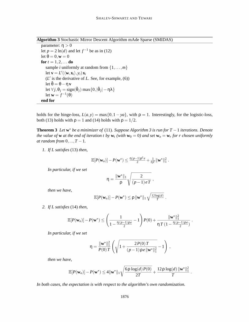
Algorithm 3 Stochastic Mirror Descent Algorithm mAde Sparse (SMIDAS)parameter:η > 0let p= 2 ln(d) and let f−1 be as in (12)let θ = 0,w = 0for t = 1,2, . . . do

samplei uniformly at random from1, . . . ,mlet v = L′(〈w,xi〉,yi)xi

(L′ is the derivative ofL. See, for example, (6))let θ = θ−ηvlet ∀ j,θ j = sign(θ j) max0, |θ j |−ηλlet w = f−1(θ)

end for

holds for the hinge-loss,L(a,y) = max0,1− ya, with ρ = 1. Interestingly, for the logistic-loss,both (13) holds withρ = 1 and (14) holds withρ = 1/2.

Theorem 3 Letw⋆ be a minimizer of(11). Suppose Algorithm 3 is run for T−1 iterations. Denotethe value ofw at the end of iteration t bywt (with w0 = 0) and setwo = wr for r chosen uniformlyat random from0, ...,T−1.

1. If L satisfies(13) then,

E[P(wo)]−P(w⋆)≤ η(p−1)ρ2 e2 + 1

ηT ‖w⋆‖21 .

In particular, if we set

η =‖w⋆‖1

ρ

√

2(p−1)eT

,

then we have,

E[P(wo)]−P(w⋆)≤ ρ‖w⋆‖1√

12log(d)T .

2. If L satisfies(14) then,

E[P(wo)]−P(w⋆)≤(

1

1− η(p−1)ρe2

−1

)

P(0)+‖w⋆‖21

ηT (1− η(p−1)ρe2 )

.

In particular, if we set

η =‖w⋆‖21P(0)T

(√

1+2P(0)T

(p−1)ρe‖w⋆‖21−1

)

,

then we have,

E[P(wo)]−P(w⋆)≤ 4‖w⋆‖1√

6ρ log(d)P(0)2T

+12ρ log(d)‖w⋆‖21

T.

In both cases, the expectation is with respect to the algorithm’s own randomization.

1876


Proof We first give the proof for the case when (13) holds. Letθt be the value ofθ at the beginningof iterationt of the algorithm, letvt be the value ofv, and letθt = θt −ηvt . Let wt = f−1(θt) andwt = f−1(θt) where f−1 is as defined in (12). Recall thatf (w) = ∇F(w) whereF(w) = 1

2‖w‖2q.Consider the Bregman divergence,

∆F(w,w′) = F(w)−F(w′)−〈∇F(w′),w−w′〉= F(w)−F(w′)−〈 f (w′),w−w′〉 ,

and define the potential,Ψ(w) = ∆F(w⋆,w) .

We first rewrite the change in potential as

Ψ(wt)−Ψ(wt+1) = (Ψ(wt)−Ψ(wt))+(Ψ(wt)−Ψ(wt+1)) , (15)

and bound each of the two summands separately.Definitions of∆F , Ψ and simple algebra yield,

Ψ(wt)−Ψ(wt) = ∆F(w⋆,wt)−∆F(w⋆, wt)

= F(wt)−F(wt)−〈 f (wt)− f (wt),w⋆〉+ 〈 f (wt),wt〉−〈 f (wt), wt〉= ∆F(wt ,wt)+ 〈 f (wt)− f (wt), wt−w⋆〉 (16)

= ∆F(wt ,wt)+ 〈θt − θt , wt −w⋆〉= ∆F(wt ,wt)+ 〈ηvt , wt−w⋆〉= ∆F(wt ,wt)+ 〈ηvt ,wt−w⋆〉+ 〈ηvt , wt−wt〉 . (17)

By strong convexity ofF with respect to theq-norm (see, e.g., Section A.4 of Shalev-Shwartz,2007), we have

∆F(wt ,wt)≥ q−12 ‖wt −wt‖2q .

Moreover, using Fenchel-Young inequality with the conjugate functionsg(x)= q−12 ‖x‖2q andg⋆(x)=

12(q−1)‖x‖2p we have

|〈ηvt , wt −w⋆〉| ≤ η2

2(q−1)‖vt‖2p+ q−12 ‖wt −w⋆‖2q .

Plugging these into (17), we get

Ψ(wt)−Ψ(wt)≥ η〈vt ,wt −w⋆〉− η2

2(q−1)‖vt‖2p= η〈vt ,wt −w⋆〉− η2(p−1)

2 ‖vt‖2p .

By convexity ofL, we have,

〈vt ,wt−w⋆〉 ≥ L(〈wt ,xi〉,yi)−L(〈w⋆,xi〉,yi) ,

and therefore

Ψ(wt)−Ψ(wt)≥ η(L(〈wt ,xi〉,yi)−L(〈w⋆,xi〉,yi))− η2(p−1)2 ‖vt‖2p .

1877


From (13), we obtain that

‖vt‖2p≤(

‖vt‖∞ d1/p)2≤ ρ2d2/p = ρ2e . (18)

Thus,Ψ(wt)−Ψ(wt)≥ η(L(〈wt ,xi〉,yi)−L(〈w⋆,xi〉,yi))− η2 (p−1)ρ2 e

2 . (19)

So far, our analysis has followed the standard analysis of mirror descent (see, e.g., Beck andTeboulle, 2003). It is a bit more tricky to show that

Ψ(wt)−Ψ(wt+1)≥ ηλ(‖wt+1‖1−‖w⋆‖1) . (20)

To show this, we begin the same way as we did to obtain (16),

Ψ(wt)−Ψ(wt+1) = ∆F(wt+1, wt)+ 〈 f (wt)− f (wt+1),wt+1−w⋆〉= ∆F(wt+1, wt)+ 〈θt −θt+1,wt+1−w⋆〉≥ 〈θt −θt+1,wt+1−w⋆〉= 〈θt −θt+1,wt+1〉−〈θt −θt+1,w⋆〉 . (21)

Note that sign(wt+1, j) = sign(θt+1, j). Moreover, whenθt+1, j 6= 0 then,

θt, j −θt+1, j = ηλsign(θt+1, j) .

Thus, we have,

〈θt −θt+1,wt+1〉= ∑j:wt+1, j 6=0

(θt, j −θt+1, j)wt+1, j

= ∑j:wt+1, j 6=0

ηλsign(θt+1, j)wt+1, j

= ηλ ∑j:wt+1, j 6=0

sign(wt+1, j)wt+1, j

= ηλ‖wt+1‖1 .

Note that this equality is crucial and does not hold for the Bregman potential corresponding to theexponentiated gradient algorithm. Plugging the above equality, along with the inequality,

|〈θt −θt+1,w⋆〉| ≤ ‖θt −θt+1‖∞‖w⋆‖1 = ηλ‖w⋆‖1

into (21), we get (20).Combining the lower bounds (19) and (20) and plugging them into (15), we get,

Ψ(wt)−Ψ(wt+1)≥ η(L(〈wt ,xi〉,yi)−L(〈w⋆,xi〉,yi))

− η2 (p−1)ρ2 e2 +ηλ(‖wt+1‖1−‖w⋆‖1) .

Taking expectation with respect toi drawn uniformly at random from1, . . . ,m, we get,

E[Ψ(wt)−Ψ(wt+1)]≥ ηE[C(wt)−C(w⋆)]− η2 (p−1)ρ2 e2 +ηλE[‖wt+1‖1−‖w⋆‖1]

= ηE[P(wt)−P(w⋆)]− η2 (p−1)ρ2 e2 +ηλE[‖wt+1‖1−‖wt‖1] .

1878


Summing overt = 0, . . . ,T−1, dividing byηT, and rearranging gives,

1T

T−1

∑t=0

E[P(wt)]−P(w⋆)≤ η(p−1)ρ2 e2 + λ

T E [‖w0‖1−‖wT‖1]+ 1ηT E [Ψ(w0)−Ψ(wT)]

≤ η(p−1)ρ2 e2 +0+ 1

ηT ∆F(w⋆,0)

= η(p−1)ρ2 e2 + 1

ηT ‖w⋆‖2q

≤ η(p−1)ρ2 e2 + 1

ηT ‖w⋆‖21 . (22)

Now, optimizing overη gives

1T

T−1

∑t=0

E[P(wt)]−P(w⋆)≤ ρ‖w⋆‖1√

2(p−1)eT

and this concludes our proof for the case when (13) holds, since for arandomr we haveE[P(wr)] =1T ∑T−1

t=0 E[P(wt)].When (14) holds, instead of the bound (18), we have,

‖vt‖2p≤(

‖vt‖∞ d1/p)2≤ ρL(〈wt ,xi〉,yi)d2/p = ρL(〈wt ,xi〉,yi)e .

As a result, the final bound (22) now becomes,

1T

T−1

∑t=0

E[P(wt)]−P(w⋆)≤ η(p−1)ρe2T

T−1

∑t=0

E[C(wt)]+1

ηT ‖w⋆‖21

≤ η(p−1)ρe2T

T−1

∑t=0

E[P(wt)]+1

ηT ‖w⋆‖21 .

For the sake of brevity, leta= (p−1)ρe/2 andb= ‖w⋆‖21, so that the above bound can be writtenas,

1T

T−1

∑t=0

E[P(wt)]−P(w⋆)≤(

11−aη

−1

)

P(w⋆)+b/(ηT)1−aη

(23)

≤(

11−aη

−1

)

P(0)+b/(ηT)1−aη

.

At this stage, we need to minimize the expression on the right hand side as a function of η. Thissomewhat tedious but straightforward minimization is done in Lemma 7 in Appendix B. UsingLemma 7 (withP= P(0)), we see that the right hand side is minimized by setting

η =‖w⋆‖21P(0)T

(√

1+2P(0)T

(p−1)ρe‖w⋆‖21−1

)

,

and the minimum value is upper bounded by

4‖w⋆‖1√

(p−1)ρeP(0)2T

+2(p−1)ρe‖w⋆‖21

T.

1879


This concludes the proof for the case when (14) holds.

The bound in the above theorem can be improved if (14) holds and the desired accuracy is thesame order asP(w⋆). This is the content of the next proposition.

Proposition 4 Let w⋆ be a minimizer of(11). Suppose Algorithm 3 is run for T− 1 iterations.Denote the value ofw at the beginning of iteration t bywt and setwo = wr for r chosen uniformlyat random from0, ...,T−1. If L satisfies(14)and we set

η =2

(p−1)ρe· K1+K

,

for some arbitrary K> 0, then we have,

E[P(wo)]≤ (1+K)P(w⋆)+(1+K)2

K· 3ρ log(d)‖w⋆‖21

T.

Proof Pluggingη = K/a(1+K) in (23) gives,

1T

T−1

∑t=0

E[P(wt)]−P(w⋆)≤ K P(w⋆)+(1+K)2

K· ab

T.

Recalling thatp= 2log(d), a= (p−1)ρe/2 andb= ‖w⋆‖21 concludes our proof.

4. Experiments

In this section, we provide experimental results for our algorithms on 4 data sets. We begin with adescription of the data sets following by a description of the algorithms we ran on them.

4.1 Data Sets

We consider 4 binary classification data sets for our experiments:DUKE, ARCENE, MAGIC04S, andMAGIC04D.

DUKE is a breast cancer data set from West et al. (2001). It has 44 examples with 7,129 fea-tures with a density level of 100%.ARCENE is a data set from the UCI Machine Learning repos-itory where the task is to distinguish cancer patterns from normal ones based on 10,000 mass-spectrometric features. Out of these, 3,000 features are synthetic features as this data set wasdesigned for the NIPS 2003 variable selection workshop. There are 100 examples in this data setand the example matrix contains 5.4× 105 non-zero entries corresponding to a density level of54%. The data setsMAGIC04S andMAGIC04D were obtained by adding 1,000 random features tothe MAGIC Gamma Telescope data set from the UCI Machine Learning repository. The originaldata set has 19,020 examples with 10 features. This is also a binary classification data set andthe task is to distinguish high-energy gamma particles from background usinga gamma telescope.Following the experimental setup of Langford et al. (2009), we added 1,000 random features, eachof which takes value 0 with probability 0.95 or 1 with probability 0.05, to create a sparse data set,MAGIC04S. We also created a dense data set,MAGIC04D, in which the random features took value−1 or+1, each with probability 0.5. MAGIC04S andMAGIC04D have density levels of 5.81% and100% respectively.

1880


4.2 Algorithms

We ran 4 algorithms on these data sets: SCD, GCD, SMIDAS, and TRUNCGRAD. SCD is thestochastic coordinate descent algorithm given in Section 2 above. GCD is the corresponding deter-ministic and “greedy” version of the same algorithm. The coordinate to be updated at each iterationis greedilychosen in a deterministic manner to maximize a lower bound on the guaranteed decreasein the objective function. This type of deterministic criterion for choosing features is common inBoosting approaches. Since choosing a coordinate (or feature in our case) in a deterministic mannerinvolves significant computation in case of large data sets, we expect that the deterministic algo-rithm will converge much slower than the stochastic algorithm. We also tried thecyclic version ofcoordinate descent that just cycles through the coordinates. We foundits performance to be indis-tinguishable from that of SCD and hence we do not report it here. SMIDAS is the mirror descentalgorithm given in Section 3 above. TRUNCGRAD is the truncated gradient algorithm of Langfordet al. (2009) (In fact, Langford et al., 2009 suggests another way to truncate the gradient. Here,we refer to the variant corresponding to SMIDAS.) Of these 4, the first two are parameter-freealgorithms while the latter two require a parameterη. In our experiments, we ran SMIDAS andTRUNCGRAD for a range of different values ofη and chose the one that yielded the minimum valueof the objective function (i.e., the regularized loss). We chose to minimize the (regularized) logisticloss in all our experiments.

4.3 Results

For each data set, we show two plots. One plot shows the regularized objective function plottedagainst the number ofdata accesses, that is, the number of times the algorithm accesses the datamatrix (xi, j). We choose to use this as opposed to, say CPU time, as this is an implementation inde-pendent quantity. Moreover, the actual time taken by these algorithms will be roughly proportionalto this quantity provided computing features is time consuming. The second plot shows the den-sity (or ℓ0-norm, the number of non-zero entries) of the iterate plotted against the number of dataaccesses. In the next subsection, we use mild regularization (λ = 10−6). Later on, we will showresults for stronger regularization (λ = 10−2).

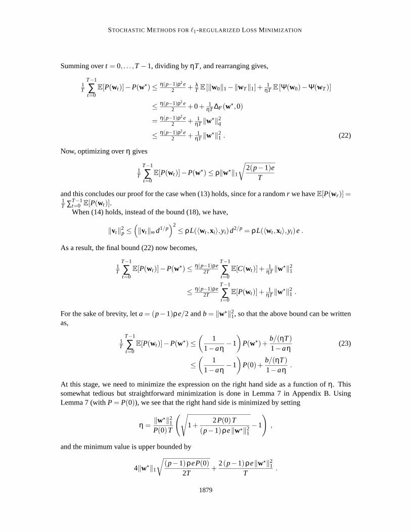
4.3.1 LESSREGULARIZATION

Figure 1 is for theDUKE data set. It is clear that GCD does much worse than the other threealgorithms. GCD is much slower because, as we mentioned above, it spends alot of time in findingthe best coordinate to update. The two algorithms having a tunable parameterη have roughly thesame performance as SCD. However, SCD has a definite edge if we add upthe time to performseveral runs of these algorithms for tuningη. Note, however, that SMIDAS has better sparsityproperties as compared to TRUNCGRAD and SCD even though their performance measured in theobjective is similar.

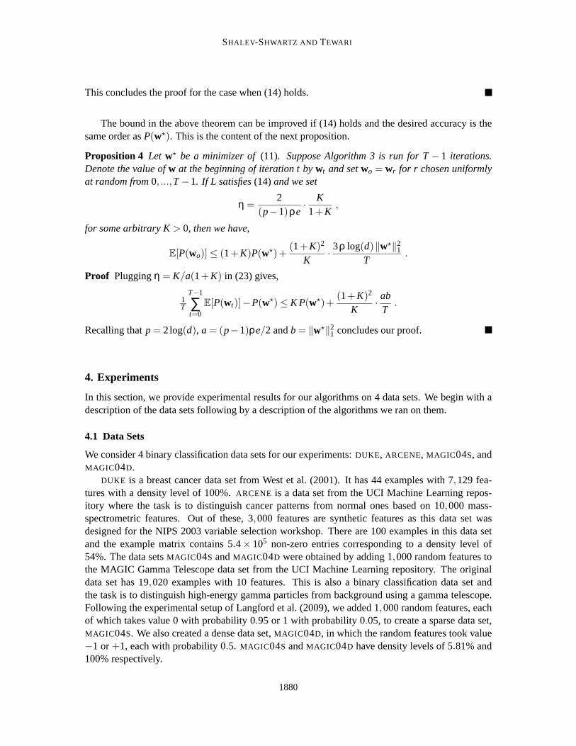
Figure 2 is for theARCENEdata set. The results are quite similar to those for theDUKE data set.SMIDAS is slow for a short while early on but quickly catches up. Again, itdisplays good sparsityproperties.

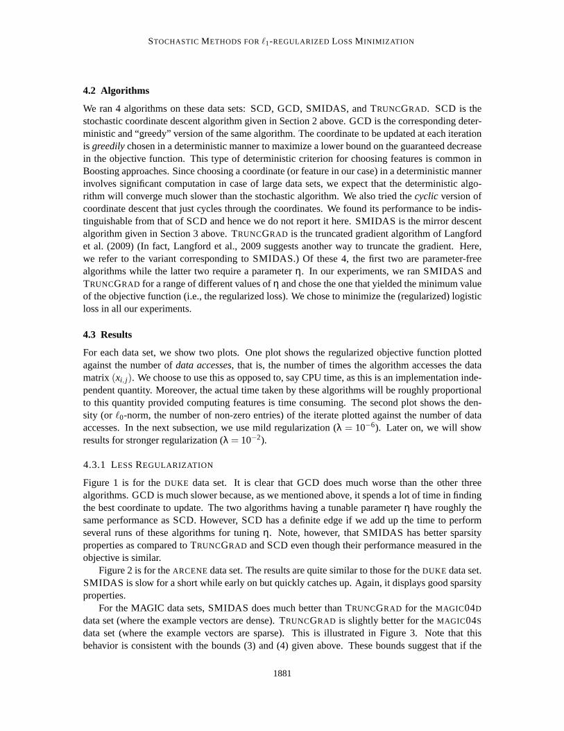
For the MAGIC data sets, SMIDAS does much better than TRUNCGRAD for the MAGIC04D

data set (where the example vectors are dense). TRUNCGRAD is slightly better for theMAGIC04S

data set (where the example vectors are sparse). This is illustrated in Figure 3. Note that thisbehavior is consistent with the bounds (3) and (4) given above. Thesebounds suggest that if the

1881


Figure 1:DUKE data set; less regularization

Figure 2:ARCENE data set; less regularization

Figure 3:MAGIC04S data set; less regularization

1882


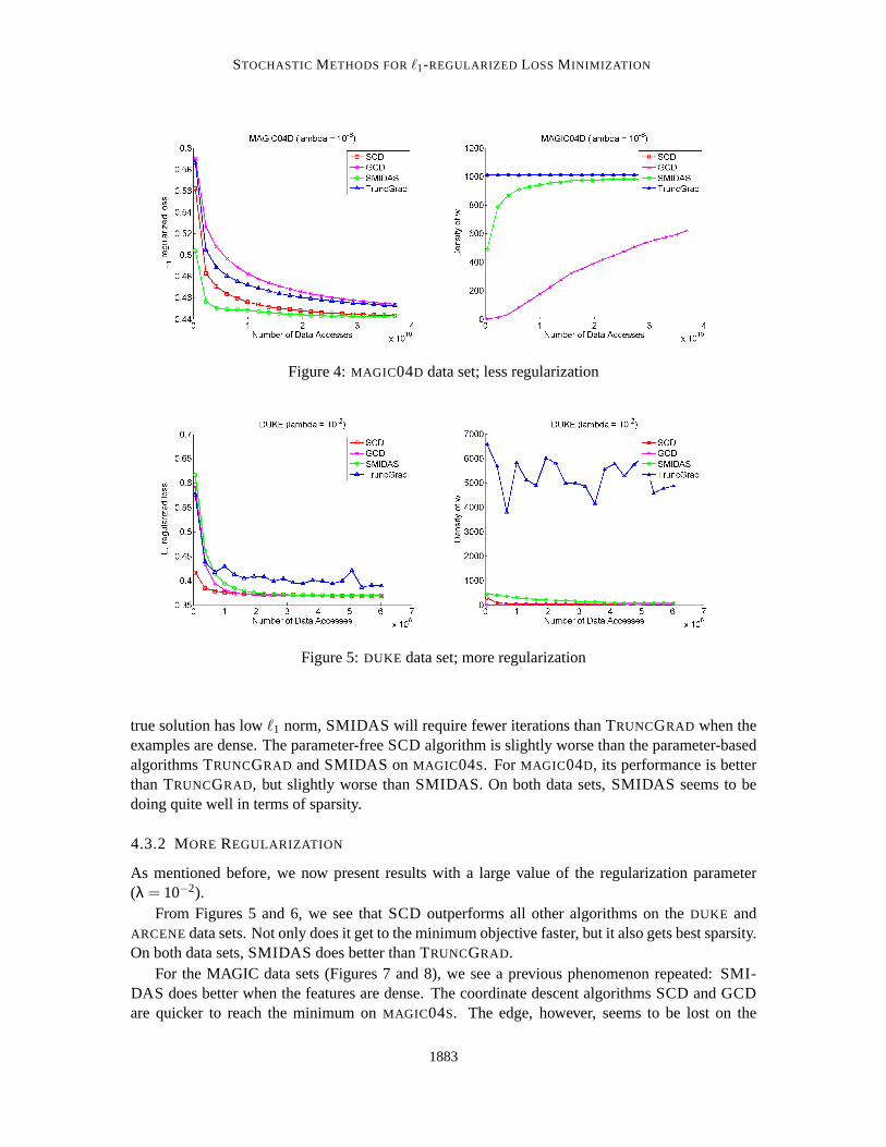
Figure 4:MAGIC04D data set; less regularization

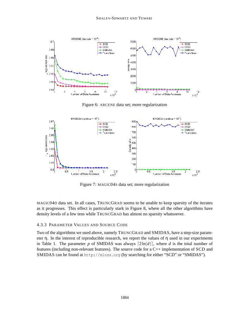
Figure 5:DUKE data set; more regularization

true solution has lowℓ1 norm, SMIDAS will require fewer iterations than TRUNCGRAD when theexamples are dense. The parameter-free SCD algorithm is slightly worse than the parameter-basedalgorithms TRUNCGRAD and SMIDAS onMAGIC04S. For MAGIC04D, its performance is betterthan TRUNCGRAD, but slightly worse than SMIDAS. On both data sets, SMIDAS seems to bedoing quite well in terms of sparsity.

4.3.2 MORE REGULARIZATION

As mentioned before, we now present results with a large value of the regularization parameter(λ = 10−2).

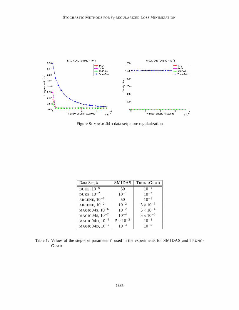
From Figures 5 and 6, we see that SCD outperforms all other algorithms on the DUKE andARCENEdata sets. Not only does it get to the minimum objective faster, but it also gets best sparsity.On both data sets, SMIDAS does better than TRUNCGRAD.

For the MAGIC data sets (Figures 7 and 8), we see a previous phenomenon repeated: SMI-DAS does better when the features are dense. The coordinate descentalgorithms SCD and GCDare quicker to reach the minimum onMAGIC04S. The edge, however, seems to be lost on the

1883


Figure 6:ARCENE data set; more regularization

Figure 7:MAGIC04S data set; more regularization

MAGIC04D data set. In all cases, TRUNCGRAD seems to be unable to keep sparsity of the iteratesas it progresses. This effect is particularly stark in Figure 8, where allthe other algorithms havedensity levels of a few tens while TRUNCGRAD has almost no sparsity whatsoever.

4.3.3 PARAMETER VALUES AND SOURCECODE

Two of the algorithms we used above, namely TRUNCGRAD and SMIDAS, have a step-size param-eterη. In the interest of reproducible research, we report the values ofη used in our experimentsin Table 1. The parameterp of SMIDAS was always⌈2ln(d)⌉, whered is the total number offeatures (including non-relevant features). The source code for aC++ implementation of SCD andSMIDAS can be found athttp://mloss.org (by searching for either “SCD” or “SMIDAS”).

1884


Figure 8:MAGIC04D data set; more regularization

Data Set,λ SMIDAS TRUNCGRAD

DUKE, 10−6 50 10−1

DUKE, 10−2 10−1 10−2

ARCENE, 10−6 50 10−1

ARCENE, 10−2 10−2 5×10−5

MAGIC04S, 10−6 10−2 5×10−4

MAGIC04S, 10−2 10−4 5×10−5

MAGIC04D, 10−6 5×10−3 10−4

MAGIC04D, 10−2 10−3 10−5

Table 1: Values of the step-size parameterη used in the experiments for SMIDAS and TRUNC-GRAD

1885


Acknowledgments

We thank Jonathan Chang for pointing out some errors in the preliminary conference version of thiswork. Most of the research reported in this paper was done while the authors were at the ToyotaTechnological Institute at Chicago (TTIC). We are grateful to TTIC forproviding a friendly andstimulating environment to work in.

Appendix A.

Lemma 5 Let ε≤ 0.12. There exists an optimization problem of the form:

minw∈Rd : ‖w‖1≤B

1m

m

∑i=1

L(〈w,xi〉,yi) ,

where L is the smooth loss function L(a,b) = (a− b)2, such that any algorithm which initializesw = 0 and updates a single element of the vectorw at each iteration, must perform at least B2/16εiterations to achieve anε accurate solution.

Proof We denote the number of non-zeros elements of a vectorw by ‖w‖0. Recall that we denotethe average loss byC(w) = 1

m ∑mi=1L(〈w,xi〉,yi). We show an optimization problem of the form

given above, for which the optimal solution, denotedw⋆, is dense (i.e.,‖w⋆‖0 = d), while anyw forwhich

C(w)≤C(w⋆)+ ε

must satisfy‖w‖0 ≥ Ω(B2/ε). This implies the statement given in the lemma since an iterationbound for the type of algorithms we consider is immediately translated into an upper bound on‖w‖0.

Let L(a,b) = (a−b)2 and consider the following joint distribution over random variables(X,Y).First, eachY is chosen at random according toP[Y = 1] = P[Y =−1] = 1

2. Next, each elementj ofX is chosen i.i.d. from+1,−1 according toP[Xj = y|y] = 1

2 +1

2B. This definition implies that:

EXj |Y=y[Xj ] =1B y

andVarXj |Y=y[Xj ] = 1− 1

B2 .

Consider the vectorw0 = (Bd , . . . ,

Bd ). We have

E[(〈w0,X〉−Y)2]= EYEX|Y=y

[(〈w0,X〉−y)2]

= EYVarX|Y=y [〈w0,X〉]

= EYB2

dVarX1|Y=y [X1]

= EYB2

d

(1− 1

B2

)

=B2−1

d.

1886


Now fix somew with ‖w‖0≤ s. We have

µy := EX|Y=y[〈w,X〉] = yB ∑

j

w j ,

and

E[(〈w,X〉−Y)2]= EYEX|Y=y

[(〈w,X〉−y)2]

= EYVarX|Y=y[〈w,X〉]+ (µy−y)2

If |∑ j w j | ≤ B/2 then(µy−y)2 ≥ 1/4 and thus we obtain from the above thatE[(〈w,X〉−Y)2

]≥

1/4. Otherwise,√

s∑j

w2j ≥∑

j

|w j | ≥ |∑j

w j | ≥ B/2 ,

and thus we have that

E[(〈w,X〉−Y)2]≥ EYVarX|Y=y [〈w,X〉]

= EY

d

∑j=1

w2j VarX1|Y=y [X1]

= EY

d

∑j=1

w2j

(1− 1

B2

)

=(1− 1

B2

) d

∑j=1

w2j

≥(1− 1

B2

)B2

4s =B2−1

4s.

ChooseB≥ 2 andd = 100(B2−1), we have shown that if‖w‖0≤ s then

E[(〈w,X〉−Y)2− (〈w0,X〉−Y)2]≥min

0.24, B2

8s

=: ε′ .

Now, consider the random variableZ = (〈w,X〉 −Y)2− (〈w0,X〉 −Y)2. This is a bounded ran-dom variable (because|〈w,x〉| ≤ B) and therefore using Hoeffding inequality we have that withprobability of at least 1−δ over a draw of a training set ofmexamples we have

C(w)−C(w0)≥ ε′−cB2

√

log(1/δ)m

,

for some universal constantc> 0.This is true if we first fixw and then draw them samples. We want to establish an inequality

true for anyw inW := w ∈ R

d : ‖w‖0≤ s, ‖w‖1≤ B .This set has infinitely many elements so we cannot trivially appeal to a union bound. Instead, wecreate anε′/16B-cover ofW in the ℓ1 metric. This has sizeN1(W ,ε′/16B) where we have thecrude estimate,

∀ε > 0, N1(W ,ε)≤ ds(

2Bdε

)s

.

1887


Moreover, if ‖w−w′‖1 ≤ ε′/16B then it is easy to see that|C(w)−C(w′)| ≤ ε′/4. Therefore,applying a union bound over all vectors in the cover, we obtain that with probability at least 1− δ,for all suchw ∈W we have

C(w)−C(w0)≥ ε′− ε′/4−cB2

√

logN1(W ,ε′/16B)+ log(1/δ)m

.

Takingm large enough, we can guarantee that, with high probability, for allw ∈W ,

C(w)−C(w0)≥ ε′/2 .

Finally, we clearly have thatC(w⋆)≤C(w0).Thus, we have proved the following. GivenB≥ 2 ands, there exist(xi ,yi)mi=1 in some dimen-

siond, such thatmin

‖w‖1≤B,‖w‖0≤sC(w)− min

‖w‖1≤BC(w)≥min

0.12, B2

16s

.

This concludes the proof of the lemma.

Appendix B.

Lemma 6 Let C be as defined in(5) and assume that the second derivative of L with respect to itsfirst argument is bounded byβ. Then, for any j∈ [d],

C(w+ηej)≤C(w)+η(∇C(w)) j +βη2

2 .

Proof Note that, by assumption onL, for anyi, j we have,

L(〈w+ηej ,xi〉,yi) = L(〈w,xi〉+ηxi, j ,yi)

≤ L(〈w,xi〉,yi)+ηL′(〈w,xi〉,yi)xi, j +βη2 x2

i, j

2

≤ L(〈w,xi〉,yi)+ηL′(〈w,xi〉,yi)xi, j +βη2

2 ,

where the last inequality follows becausexi, j ∈ [−1,+1]. Adding the above inequalities fori =1, . . . ,mand dividing bym, we get

C(w+ηej)≤C(w)+ηm

m

∑i=1

L′(〈w,xi〉,yi)xi, j +βη2

2

=C(w)+η(∇C(w)) j +βη2

2 .

Lemma 7 Let a,b,P,T > 0. The function f: (0,1/a)→ R defined as,

f (η) =(

11−aη

−1

)

P+b/(ηT)1−aη

1888


is minimized at

η⋆ =b

PT

(√

1+PTab−1

)

,

and the minimum value satisfies

f (η⋆)≤ 4

√

abPT

+4abT

.

Proof A little rearranging gives,

f (η) =1

1η −a

(

aP+b

η2T

)

.

This suggests the change of variableC= 1/η and we wish to minimizeg : (a,∞)→ R defined as,

g(C) =1

C−a

(

aP+bC2

T

)

.

The expression for the derivativeg′ is,

g′(C) =b

T(C−a)2

(

C2−2aC− aTPb

)

.

Settingg′(C) = 0 gives a quadratic equation whose roots are,

a±√

a2+aTP

b.

Choosing the larger root (the smaller one is smaller thana) gives us the minimizer,

C⋆ = a+

√

a2+aTP

b.

It is easy to see thatg′(C) is increasing atC⋆ and thus we have a local minima atC⋆ (which is alsoglobal in this case). The minimizerη⋆ of f (η) is therefore,

η⋆ =1

C⋆=

bPT

(√

1+PTab−1

)

.

Plugging in the value ofC⋆ into g(C), we get,

g(C⋆) =2

√

1+ PTab

(

P+abT

+

√

a2b2

T2 +abPT

)

≤ 2√

1+ PTab

(

2P+2abT

)

= 4

√

abPT

+a2b2

T2

≤ 4

√

abPT

+4abT

.

Sinceg(C⋆) = f (η⋆), this concludes the proof of the lemma.

1889


References

A. Beck and M. Teboulle. Mirror descent and nonlinear projected subgradient methods for convexoptimization.Operations Research Letters, 31:167–175, 2003.

L. Bottou. Stochastic gradient descent examples, Web Page.http://leon.bottou.org/projects/sgd.

L. Bottou and O. Bousquet. The tradeoffs of large scale learning. InAdvances in Neural InformationProcessing Systems 20, pages 161–168, 2008.

L. Bottou and Y. LeCunn. On-line learning for very large datasets.Applied Stochastic Models inBusiness and Industry, 21(2):137–151, 2005.

K.L. Clarkson. Coresets, sparse greedy approximation, and the Frank-Wolfe algorithm. InProceed-ings of the nineteenth annual ACM-SIAM symposium on Discrete algorithms, pages 922–931,2008.

N. Cristianini and J. Shawe-Taylor.An Introduction to Support Vector Machines. Cambridge Uni-versity Press, 2000.

J. Duchi, S. Shalev-Shwartz, Y. Singer, and T. Chandra. Efficient projections onto theℓ1-ball forlearning in high dimensions. InInternational Conference on Machine Learning, pages 272–279,2008.

J. Duchi, S. Shalev-Shwartz, Y. Singer, and A. Tewari. Composite objective mirror descent. InProceedings of the 23rd Annual Conference on Learning Theory, pages 14–26, 2010.

B. Efron, T. Hastie, I. Johnstone, and R. Tibshirani. Least angle regression.Annals of Statistics, 32(2):407–499, 2004.

M. Frank and P. Wolfe. An algorithm for quadratic programming.Naval Research Logistics Quar-terly, 3:95–110, 1956.

J. Friedman, T. Hastie, and R. Tibshirani. Regularized paths for generalized linear models viacoordinate descent.Journal of Statistical Software, 33(1):1–22, 2010.

A. Genkin, D. Lewis, and D. Madigan. Large-scale Bayesian logistic regression for text categoriza-tion. Technometrics, 49(3):291–304, 2007.

C. Gentile. The robustness of the p-norm algorithms.Machine Learning, 53(3):265–299, 2003.

S. Ghadimi and G. Lan. Optimal stochastic approximation algorithms for stronglyconvex stochas-tic composite optimization, 2011. available athttp://www.ise.ufl.edu/glan/papers/strongSCOSubmit.pdf.

A. J. Grove, N. Littlestone, and D. Schuurmans. General convergence results for linear discriminantupdates.Machine Learning, 43(3):173–210, 2001.

J. Kivinen and M. Warmuth. Exponentiated gradient versus gradient descent for linear predictors.Information and Computation, 132(1):1–64, January 1997.

1890


K. Koh, S.J. Kim, and S. Boyd. An interior-point method for large-scaleℓ1-regularized logisticregression.Journal of Machine Learning Research, 8:1519–1555, 2007.

G. Lan. An optimal method for stochastic composite optimization.Mathematical Programming,pages 1–33, 2010.

J. Langford, L. Li, and T. Zhang. Sparse online learning via truncatedgradient. InAdvances inNeural Information Processing Systems 21, pages 905–912, 2009.

N. Littlestone. Learning quickly when irrelevant attributes abound: A new linear-threshold algo-rithm. Machine Learning, 2:285–318, 1988.

Z. Q. Luo and P. Tseng. On the convergence of coordinate descent method for convex differentiableminimization.Journal of Optimization Theory and Applications, 72:7–35, 1992.

A. Nemirovski and D. Yudin.Problem complexity and method efficiency in optimization. NaukaPublishers, Moscow, 1978.

Y. Nesterov. Efficiency of coordinate descent methods on huge-scaleoptimization problems. Tech-nical Report CORE Discussion Paper 2010/02, Center for Operations Research and Economet-rics, UCL, Belgium, 2010.

S. Shalev-Shwartz.Online Learning: Theory, Algorithms, and Applications. PhD thesis, TheHebrew University, 2007.

S. Shalev-Shwartz and N. Srebro. SVM optimization: Inverse dependence on training set size. InInternational Conference on Machine Learning, pages 928–935, 2008.

S. Shalev-Shwartz and A. Tewari. Stochastic methods forℓ1 regularized loss minimization. InInternational Conference on Machine Learning, pages 929–936, 2009.

S. Shalev-Shwartz, Y. Singer, and N. Srebro. Pegasos: Primal Estimated sub-GrAdient SOlver forSVM. In International Conference on Machine Learning, pages 807–814, 2007.

S. Shalev-Shwartz, T. Zhang, and N. Srebro. Trading accuracy for sparsity in optimization problemswith sparsity constraints.SIAM Journal on Optimization, 20:2807–2832, 2010.

R. Tibshirani. Regression shrinkage and selection via the lasso.Journal of the Royal StatisticalSociety: Series B, 58(1):267–288, 1996.

P. Tseng and S. Yun. A block-coordinate gradient descent method forlinearly constrained nons-mooth separable optimization.Journal of Optimization Theory and Applications, 140:513–535,2009.

M. West, C. Blanchette, H. Dressman, E. Huang, S. Ishida, R. Spang, H. Zuzan, J. A. Olson, J. R.Marks, and J. R. Nevins. Predicting the clinical status of human breast cancer by using geneexpression profiles.Proceedings of the National Academy of Sciences USA, 98(20):11462–11467,2001.

T. T. Wu and K. Lange. Coordinate descent algorithms for lasso penalized regression.Annals ofApplied Statistics, 2(1):224–244, 2008.

1891


L. Xiao. Dual averaging method for regularized stochastic learning and online optimization.Journalof Machine Learning Research, 11:2543–2596, 2010.

T. Zhang. Sequential greedy approximation for certain convex optimizationproblems.IEEE Trans-action on Information Theory, 49:682–691, 2003.

T. Zhang and F. J. Oles. Text categorization based on regularized linear classification methods.Information Retrieval, 4:5–31, 2001.

1892

Documents

Stochastic Methods for ℓ1-regularized Loss Minimization ...jmlr.org/papers/volume12/shalev-shwartz11a/shalev-shwartz11a.pdf · convex optimization problem, and therefore can be