Embed Size (px)
Citation preview
Multistage stochastic programming Dynamic Programming Numerical aspects Discussion
Stochastic Dynamic Programming
V. Leclere (ENPC)F. Pacaud, T.Rigaut (Efficacity)
March 14, 2017
Leclere, Pacaud, Rigaut Dynamic Programming March 14, 2017 1 / 22

Multistage stochastic programming Dynamic Programming Numerical aspects Discussion
Contents
1 Multistage stochastic programmingFrom two-stage to multistage programmingCompressing information inside a state
2 Dynamic ProgrammingOptimization problemDynamic Programming principle
3 Numerical aspectsCurses of dimensionalityMarkov chain setting
4 Discussion
Leclere, Pacaud, Rigaut Dynamic Programming March 14, 2017 2 / 22
Multistage stochastic programming Dynamic Programming Numerical aspects Discussion
Where do we come from: two-stage programming
u0
(w 11 , π1)
u1,1
(w 21 , π2)
u1,2
(w 31 , π3)
u1,3
(w 41 , π4)
u1,4
(w 51 , π5) u1,5
(w 61 , π6)
u1,6
(w 71 , π7)
u1,7(w 8
1 , π8)
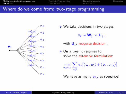
u1,8 We take decisions in two stages
u0 ; W1 ; U1 ,
with U1: recourse decision .
On a tree, it resumes tosolve the extensive formulation:
minu0,u1,s
∑s∈S
πs[⟨
cs , u0
⟩+⟨ps , u1,s
⟩].
We have as many u1,s as scenarios!
Leclere, Pacaud, Rigaut Dynamic Programming March 14, 2017 3 / 22

Multistage stochastic programming Dynamic Programming Numerical aspects Discussion
Extending two-stage to multistage programming
u0
(w 11 , π1)
u11
u1,12
u1,22
u1,32
u1,42
(w 21 , π2)u2
1
u2,12
u2,22
u2,32
u2,42
(w 31 , π3)
u31
u3,12
u3,22
u3,32
u3,42
(w 41 , π4)
u41
u4,12
u4,22
u4,32
u4,42 min
UE(j(U,W)
)U = (U0, · · · ,UT )
W = (W1, · · · ,WT )
We take decisions in T stages
W0 ; U0 ; W1 ; U1 ; · · ·; WT ; UT .
Leclere, Pacaud, Rigaut Dynamic Programming March 14, 2017 4 / 22

Multistage stochastic programming Dynamic Programming Numerical aspects Discussion
Introducing the non-anticipativity constraint
We do not know what holds behind the door.
Non-anticipativity
At time t, decisions are taken sequentially, only knowing the pastrealizations of the perturbations.
Mathematically, this is equivalent to say that at time t,the decision Ut is
1 a function of past noises
Ut = πt(W0, · · · ,Wt) ,
2 taken knowing the available information,
σ(Ut) ⊂ σ(W0, · · · ,Wt) .
Leclere, Pacaud, Rigaut Dynamic Programming March 14, 2017 5 / 22

Multistage stochastic programming Dynamic Programming Numerical aspects Discussion
Multistage extensive formulation approach
u0
(w 11 , π1)
u11
u1,12
u1,22
u1,32
u1,42
(w 21 , π2)u2
1
u2,12
u2,22
u2,32
u2,42
(w 31 , π3)
u31
u3,12
u3,22
u3,32
u3,42
(w 41 , π4)
u41
u4,12
u4,22
u4,32
u4,42
Assume that wt ∈ Rnw can take nw valuesand that Ut(x) can take nu values.
Then, considering the extensive formulationapproach, we have
nTw scenarios.
(nT+1w − 1)/(nw − 1) nodes in the tree.
Number of variables in the optimizationproblem is roughlynu × (nT+1
w − 1)/(nw − 1) ≈ nunTw .
The complexity grows exponentially with thenumber of stage. :-(A way to overcome this issue is to compressinformation!
Leclere, Pacaud, Rigaut Dynamic Programming March 14, 2017 6 / 22

Multistage stochastic programming Dynamic Programming Numerical aspects Discussion
Illustrating extensive formulation with the damsvalleyexample
SoulcemGnioure Izourt
Auzat
Sabart
5 interconnected dams
5 controls per timesteps
52 timesteps (one per week, over oneyear)
nw = 10 noises for each timestep
We obtain 1052 scenarios, and ≈ 5.1052
constraints in the extensive formulation ...Estimated storage capacity of the Internet:1024 bytes.
Leclere, Pacaud, Rigaut Dynamic Programming March 14, 2017 7 / 22

Multistage stochastic programming Dynamic Programming Numerical aspects Discussion
Contents
1 Multistage stochastic programmingFrom two-stage to multistage programmingCompressing information inside a state
2 Dynamic ProgrammingOptimization problemDynamic Programming principle
3 Numerical aspectsCurses of dimensionalityMarkov chain setting
4 Discussion
Leclere, Pacaud, Rigaut Dynamic Programming March 14, 2017 7 / 22
Multistage stochastic programming Dynamic Programming Numerical aspects Discussion
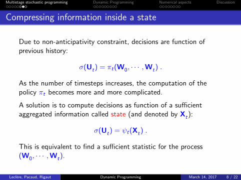
Compressing information inside a state
Due to non-anticipativity constraint, decisions are function ofprevious history:
σ(Ut) = πt(W0, · · · ,Wt) .
As the number of timesteps increases, the computation of thepolicy πt becomes more and more complicated.
A solution is to compute decisions as function of a sufficientaggregated information called state (and denoted by Xt):
σ(Ut) = ψt(Xt) .
This is equivalent to find a sufficient statistic for the process(W0, · · · ,Wt).
Leclere, Pacaud, Rigaut Dynamic Programming March 14, 2017 8 / 22

Multistage stochastic programming Dynamic Programming Numerical aspects Discussion
Contents
1 Multistage stochastic programmingFrom two-stage to multistage programmingCompressing information inside a state
2 Dynamic ProgrammingOptimization problemDynamic Programming principle
3 Numerical aspectsCurses of dimensionalityMarkov chain setting
4 Discussion
Leclere, Pacaud, Rigaut Dynamic Programming March 14, 2017 8 / 22

Multistage stochastic programming Dynamic Programming Numerical aspects Discussion
Stochastic Controlled Dynamic System
A discrete time controlled stochastic dynamic system is defined byits dynamic
Xt+1 = ft(Xt ,Ut ,Wt+1)
and initial stateX0 = W0
The variables
Xt is the state of the system,
Ut is the control applied to the system at time t,
Wt is an exogeneous noise.
Usually, Xt ∈ Xt and Ut beglongs to a set depending upon thestate: Ut ∈ Ut(Xt).
Leclere, Pacaud, Rigaut Dynamic Programming March 14, 2017 9 / 22

Multistage stochastic programming Dynamic Programming Numerical aspects Discussion
Examples
Stock of water in a dam:
Xt is the amount of water in the dam at time t,Ut is the amount of water turbined at time t,Wt+1 is the inflow of water in [t, t + 1[.
Boat in the ocean:
Xt is the position of the boat at time t,Ut is the direction and speed chosen for [t, t + 1[,Wt+1 is the wind and current for [t, t + 1[.
Subway network:
Xt is the position and speed of each train at time t,Ut is the acceleration chosen at time t,Wt+1 is the delay due to passengers and incident on thenetwork for [t, t + 1[.
Leclere, Pacaud, Rigaut Dynamic Programming March 14, 2017 10 / 22
Multistage stochastic programming Dynamic Programming Numerical aspects Discussion
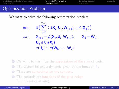
Optimization Problem
We want to solve the following optimization problem
min E( T−1∑
t=0
Lt
(Xt ,Ut ,Wt+1
)+ K
(XT
))s.t. Xt+1 = ft(Xt ,Ut ,Wt+1), X0 = W0
Ut ∈ Ut(Xt)
σ(Ut) ⊂ σ(W0, · · · ,Wt
)1 We want to minimize the expectation of the sum of costs.
2 The system follows a dynamic given by the function ft .
3 There are constraints on the controls.
4 The controls are functions of the past noises(= non-anticipativity).
Leclere, Pacaud, Rigaut Dynamic Programming March 14, 2017 11 / 22

Multistage stochastic programming Dynamic Programming Numerical aspects Discussion
Optimization Problem with independence of noises
If noises at time independent, the optimization problem isequivalent to
min E( T−1∑
t=0
Lt
(Xt ,Ut ,Wt+1
)+ K
(XT
))s.t. Xt+1 = ft(Xt ,Ut ,Wt+1), X0 = W0
Ut ∈ Ut(Xt)
Ut = ψt(Xt)
Leclere, Pacaud, Rigaut Dynamic Programming March 14, 2017 12 / 22

Multistage stochastic programming Dynamic Programming Numerical aspects Discussion
Contents
1 Multistage stochastic programmingFrom two-stage to multistage programmingCompressing information inside a state
2 Dynamic ProgrammingOptimization problemDynamic Programming principle
3 Numerical aspectsCurses of dimensionalityMarkov chain setting
4 Discussion
Leclere, Pacaud, Rigaut Dynamic Programming March 14, 2017 12 / 22
Multistage stochastic programming Dynamic Programming Numerical aspects Discussion
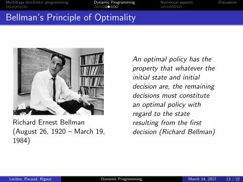
Bellman’s Principle of Optimality
Richard Ernest Bellman(August 26, 1920 – March 19,1984)
An optimal policy has theproperty that whatever theinitial state and initialdecision are, the remainingdecisions must constitutean optimal policy withregard to the stateresulting from the firstdecision (Richard Bellman)
Leclere, Pacaud, Rigaut Dynamic Programming March 14, 2017 13 / 22
Multistage stochastic programming Dynamic Programming Numerical aspects Discussion
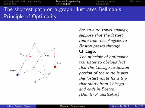
The shortest path on a graph illustrates Bellman’sPrinciple of Optimality
For an auto travel analogy,suppose that the fastestroute from Los Angeles toBoston passes throughChicago.The principle of optimalitytranslates to obvious factthat the Chicago to Bostonportion of the route is alsothe fastest route for a tripthat starts from Chicagoand ends in Boston.(Dimitri P. Bertsekas)
Leclere, Pacaud, Rigaut Dynamic Programming March 14, 2017 14 / 22
Multistage stochastic programming Dynamic Programming Numerical aspects Discussion
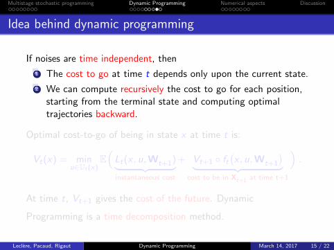
Idea behind dynamic programming
If noises are time independent, then
1 The cost to go at time t depends only upon the current state.
2 We can compute recursively the cost to go for each position,starting from the terminal state and computing optimaltrajectories backward.
Optimal cost-to-go of being in state x at time t is:
Vt(x) = minu∈Ut(x)
E(
Lt(x , u,Wt+1)︸ ︷︷ ︸instantaneous cost
+ Vt+1 ◦ ft(x , u,Wt+1
)︸ ︷︷ ︸cost to be in Xt+1 at time t+1
).
At time t, Vt+1 gives the cost of the future. Dynamic
Programming is a time decomposition method.
Leclere, Pacaud, Rigaut Dynamic Programming March 14, 2017 15 / 22

Multistage stochastic programming Dynamic Programming Numerical aspects Discussion
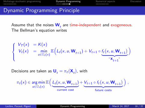
Dynamic Programming Principle
Assume that the noises Wt are time-independent and exogeneous.The Bellman’s equation writes
VT (x) = K (x)
Vt(x) = minu∈Ut(x)
E(
Lt(x , u,Wt+1) + Vt+1 ◦ ft(x , u,Wt+1
)︸ ︷︷ ︸”Xt+1”
)
Decisions are taken as Ut = πt(Xt
), with
πt(x) ∈ arg minu∈Ut(x)
E(
Lt(x , u,Wt+1)︸ ︷︷ ︸current cost
+ Vt+1 ◦ ft(x , u,Wt+1
)︸ ︷︷ ︸future costs
),
Leclere, Pacaud, Rigaut Dynamic Programming March 14, 2017 16 / 22
Multistage stochastic programming Dynamic Programming Numerical aspects Discussion
Dynamic Programming Principle
Assume that the noises Wt are time-independent and exogeneous.The Bellman’s equation writes
VT (x) = K (x)
Vt(x) = minu∈Ut(x)
E(
Lt(x , u,Wt+1) + Vt+1 ◦ ft(x , u,Wt+1
)︸ ︷︷ ︸”Xt+1”
)
Decisions are taken as Ut = πt(Xt
), with
πt(x) ∈ arg minu∈Ut(x)
E(
Lt(x , u,Wt+1)︸ ︷︷ ︸current cost
+ Vt+1 ◦ ft(x , u,Wt+1
)︸ ︷︷ ︸future costs
),
Leclere, Pacaud, Rigaut Dynamic Programming March 14, 2017 16 / 22

Multistage stochastic programming Dynamic Programming Numerical aspects Discussion
Interpretation of Bellman Value Function
The Bellman’s value function Vt0(x) can be interpreted as thevalue of the problem starting at time t0 from the state x .More precisely we have
Vt0(x) = min E( T−1∑
t=t0
Lt
(Xt ,Ut ,Wt+1
)+ K
(XT
))s.t. Xt+1 = ft(Xt ,Ut ,Wt+1), Xt0
= x
Ut ∈ Ut(Xt)
σ(Ut) ⊂ σ(W0, · · · ,Wt
)
Ex: Economists can view V as a way toevaluate a stock (= value of water for a dam)
Leclere, Pacaud, Rigaut Dynamic Programming March 14, 2017 17 / 22

Multistage stochastic programming Dynamic Programming Numerical aspects Discussion
Contents
1 Multistage stochastic programmingFrom two-stage to multistage programmingCompressing information inside a state
2 Dynamic ProgrammingOptimization problemDynamic Programming principle
3 Numerical aspectsCurses of dimensionalityMarkov chain setting
4 Discussion
Leclere, Pacaud, Rigaut Dynamic Programming March 14, 2017 17 / 22
Multistage stochastic programming Dynamic Programming Numerical aspects Discussion
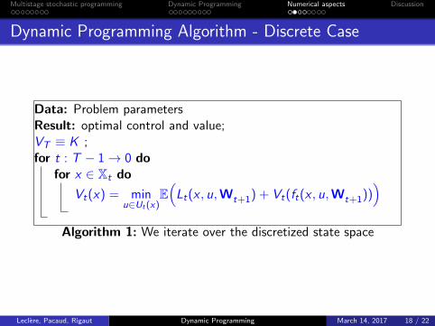
Dynamic Programming Algorithm - Discrete Case
Data: Problem parametersResult: optimal control and value;VT ≡ K ;for t : T − 1→ 0 do
for x ∈ Xt do
Vt(x) = minu∈Ut(x)
E(
Lt(x , u,Wt+1) + Vt(ft(x , u,Wt+1)))
Algorithm 1: We iterate over the discretized state space
Leclere, Pacaud, Rigaut Dynamic Programming March 14, 2017 18 / 22

Multistage stochastic programming Dynamic Programming Numerical aspects Discussion
Dynamic Programming Algorithm - Discrete Case
Data: Problem parametersResult: optimal control and value;VT ≡ K ;for t : T − 1→ 0 do
for x ∈ Xt doVt(x) =∞;for u ∈ Ut(x) do
vu = E(
Lt(x , u,Wt+1) + Vt(ft(x , u,Wt+1)))
if
vu < Vt(x) thenVt(x) = vu ;πt(x) = u ;
Algorithm 2: We iterate over the discretized control space
Leclere, Pacaud, Rigaut Dynamic Programming March 14, 2017 19 / 22

Multistage stochastic programming Dynamic Programming Numerical aspects Discussion
Dynamic Programming Algorithm - Discrete Case
Data: Problem parametersResult: optimal control and value;VT ≡ K ;for t : T − 1→ 0 do
for x ∈ Xt doVt(x) =∞;for u ∈ Ut(x) do
vu = 0;for w ∈Wt do
vu = vu + P{w}(Lt(x , u,w) + Vt+1(ft
(x , u,w
)));
if vu < Vt(x) thenVt(x) = vu ;πt(x) = u ;
Algorithm 3: Classical stochastic dynamic programming algorithm
Leclere, Pacaud, Rigaut Dynamic Programming March 14, 2017 20 / 22

Multistage stochastic programming Dynamic Programming Numerical aspects Discussion
3 curses of dimensionality
Complexity = O(T × |Xt | × |Ut | × |Wt |)
This is linear in the number of time steps :-)
But we have 3 curses of dimensionality :-( :
1 State. Complexity is exponential in the dimension of Xt
2 Decision. Complexity is exponential in the dimension of Ut
3 Expectation. Complexity is exponential in the dimension ofWt
Leclere, Pacaud, Rigaut Dynamic Programming March 14, 2017 21 / 22

Multistage stochastic programming Dynamic Programming Numerical aspects Discussion
Illustrating dynamic programming with the damsvalleyexample
SoulcemGnioure Izourt
Auzat
Sabart
Leclere, Pacaud, Rigaut Dynamic Programming March 14, 2017 22 / 22

Multistage stochastic programming Dynamic Programming Numerical aspects Discussion
Illustrating the curse of dimensionality
We are in dimension 5 (not so high in the world of big data!) with52 timesteps (common in energy management) plus 5 controls and5 independent noises.
1 We discretize each state’s dimension in 100 values:|Xt | = 1005 = 1010
2 We discretize each control’s dimension in 100 values:|Ut | = 1005 = 1010
3 We use optimal quantization to discretize the noises’ space in10 values: |Wt | = 10
Number of flops: O(52× 1010 × 1010 × 10) ≈ O(1023).In the TOP500, the best computer computes 1017 flops/s.Even with the most powerful computer, it takes at least 12 days tosolve this problem.
Leclere, Pacaud, Rigaut Dynamic Programming March 14, 2017 23 / 22

Multistage stochastic programming Dynamic Programming Numerical aspects Discussion
Contents
1 Multistage stochastic programmingFrom two-stage to multistage programmingCompressing information inside a state
2 Dynamic ProgrammingOptimization problemDynamic Programming principle
3 Numerical aspectsCurses of dimensionalityMarkov chain setting
4 Discussion
Leclere, Pacaud, Rigaut Dynamic Programming March 14, 2017 23 / 22

Multistage stochastic programming Dynamic Programming Numerical aspects Discussion
DP on a Markov Chain
Sometimes it is easier to represent a problem as a controlledMarkov Chain
Dynamic Programming equation can be computed directly,without expliciting the control.
Let’s work out an example...
Leclere, Pacaud, Rigaut Dynamic Programming March 14, 2017 24 / 22
Multistage stochastic programming Dynamic Programming Numerical aspects Discussion
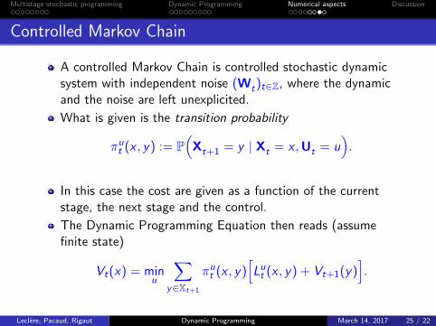
Controlled Markov Chain
A controlled Markov Chain is controlled stochastic dynamicsystem with independent noise (Wt)t∈Z, where the dynamicand the noise are left unexplicited.
What is given is the transition probability
πut (x , y) := P(
Xt+1 = y | Xt = x ,Ut = u).
In this case the cost are given as a function of the currentstage, the next stage and the control.
The Dynamic Programming Equation then reads (assumefinite state)
Vt(x) = minu
∑y∈Xt+1
πut (x , y)[Lut (x , y) + Vt+1(y)
].
Leclere, Pacaud, Rigaut Dynamic Programming March 14, 2017 25 / 22

Multistage stochastic programming Dynamic Programming Numerical aspects Discussion
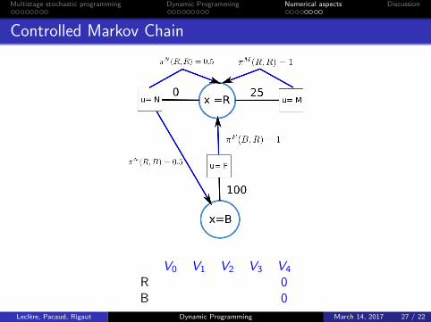
Example
Consider a machine that has two states : running (R) and broken(B). If it is broken we need to fix it (F) for a cost of 100. If it isrunning there are two choices: maintaining it (M), or notmaintaining (N). If we maintain, the cost is 25 and the machinestay running with probability πM(R,R) = 1; if we do not maintainthere is a probability of πN(R,B) = 0.5 of breaking it (or keep itrunning). We need to have it running for 3 periods.
Leclere, Pacaud, Rigaut Dynamic Programming March 14, 2017 26 / 22

Multistage stochastic programming Dynamic Programming Numerical aspects Discussion
Controlled Markov Chain
V0 V1 V2 V3 V4
R 0B 0
Leclere, Pacaud, Rigaut Dynamic Programming March 14, 2017 27 / 22
Multistage stochastic programming Dynamic Programming Numerical aspects Discussion
Controlled Markov Chain
V0 V1 V2 V3 V4
R 0B 0
Leclere, Pacaud, Rigaut Dynamic Programming March 14, 2017 27 / 22
Multistage stochastic programming Dynamic Programming Numerical aspects Discussion
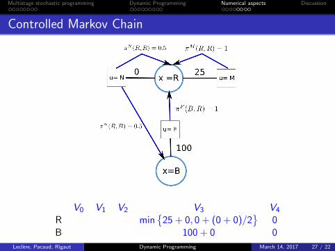
Controlled Markov Chain
V0 V1 V2 V3 V4
R min{
25 + 0, 0 + (0 + 0)/2}
0B 100 + 0 0
Leclere, Pacaud, Rigaut Dynamic Programming March 14, 2017 27 / 22

Multistage stochastic programming Dynamic Programming Numerical aspects Discussion
Controlled Markov Chain
V0 V1 V2 V3 V4
R min{
25 + 0, 0 + (0 + 100)/2}
0 0B 100 + 0 100 0
Leclere, Pacaud, Rigaut Dynamic Programming March 14, 2017 27 / 22

Multistage stochastic programming Dynamic Programming Numerical aspects Discussion
Controlled Markov Chain
V0 V1 V2 V3 V4
R min{
25 + 25, 0 + (25 + 100)/2}
25 0 0B 100 + 25 100 100 0
Leclere, Pacaud, Rigaut Dynamic Programming March 14, 2017 27 / 22

Multistage stochastic programming Dynamic Programming Numerical aspects Discussion
Controlled Markov Chain
V0 V1 V2 V3 V4
R min{
25 + 50, 0 + (50 + 125)/2}
50 25 0 0B 100 + 50 125 100 100 0
Leclere, Pacaud, Rigaut Dynamic Programming March 14, 2017 27 / 22

Multistage stochastic programming Dynamic Programming Numerical aspects Discussion
Controlled Markov Chain
V0 V1 V2 V3 V4
R 75 50 25 0 0B 150 125 100 100 0
Leclere, Pacaud, Rigaut Dynamic Programming March 14, 2017 27 / 22

Multistage stochastic programming Dynamic Programming Numerical aspects Discussion
Contents
1 Multistage stochastic programmingFrom two-stage to multistage programmingCompressing information inside a state
2 Dynamic ProgrammingOptimization problemDynamic Programming principle
3 Numerical aspectsCurses of dimensionalityMarkov chain setting
4 Discussion
Leclere, Pacaud, Rigaut Dynamic Programming March 14, 2017 27 / 22

Multistage stochastic programming Dynamic Programming Numerical aspects Discussion
Computing a decision online
Algorithm: Offline value functions precomputation + Online openloop reoptimization
Offline: We produce value functions with Bellman equation:
Vt(x) = minu∈Ut
E(
Lt(x , u,Wt+1) + Vt+1(ft(x , u,Wt+1)))
Online: At time t, knowing xt we plug the computed valuefunction Vt+1 as future cost
ut ∈ arg minu∈Ut
E(
Lt(xt , u,Wt+1) + Vt+1(ft(xt , u,Wt+1)))
Leclere, Pacaud, Rigaut Dynamic Programming March 14, 2017 28 / 22
Multistage stochastic programming Dynamic Programming Numerical aspects Discussion
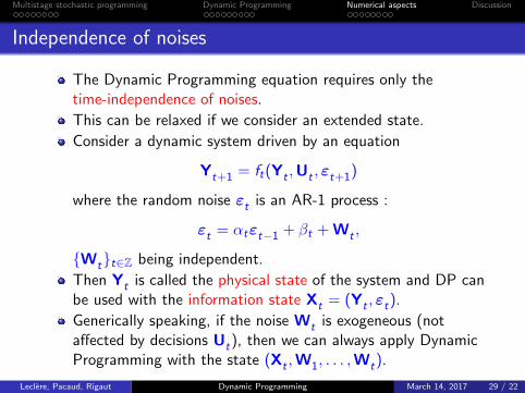
Independence of noises
The Dynamic Programming equation requires only thetime-independence of noises.
This can be relaxed if we consider an extended state.
Consider a dynamic system driven by an equation
Yt+1 = ft(Yt ,Ut , εt+1)
where the random noise εt is an AR-1 process :
εt = αtεt−1 + βt + Wt ,
{Wt}t∈Z being independent.
Then Yt is called the physical state of the system and DP canbe used with the information state Xt = (Yt , εt).
Generically speaking, if the noise Wt is exogeneous (notaffected by decisions Ut), then we can always apply DynamicProgramming with the state (Xt ,W1, . . . ,Wt).
Leclere, Pacaud, Rigaut Dynamic Programming March 14, 2017 29 / 22

Multistage stochastic programming Dynamic Programming Numerical aspects Discussion
State augmentation limits
Because of the curse of dimensionality it might be impossible totake into account correlation by augmenting the state variable.
Practitioners often ignore noise dependence for the value functionscomputation but use dependence information during onlinereoptimization.
We present this technique in a following industrial casepresentation
Leclere, Pacaud, Rigaut Dynamic Programming March 14, 2017 30 / 22

Multistage stochastic programming Dynamic Programming Numerical aspects Discussion
Conclusion
Multistage stochastic programming fails to handle largenumber of timesteps.
Dynamic Programming overcomes this difficulty whilecompressing information inside a state X.
Dynamic Programming computes backward a set of valuefunctions
{Vt
}, corresponding to the optimal cost of being at
a given position at time t.
Numerically, DP is limited by the curse of dimensionality andits performance are deeply related to the discretization of thelook-up table used.
Other methods exist to compute the value functions withoutlook-up table (Approximate Dynamic Programming, SDDP).
Leclere, Pacaud, Rigaut Dynamic Programming March 14, 2017 31 / 22

Independence of noises: AR-1 case
Consider a dynamic system driven by an equationYt+1 = ft(Yt ,Ut , εt+1) where the random noise εt is anAR-1 process : εt = αtεt−1 + βt + Wt+1, {Wt}t∈Z beingindependent.
Define the information state Xt = (Yt , εt).
Then we have
Xt+1 =
(ft(Yt ,Ut , αtεt + βt + Wt+1)
αtεt + βt + Wt+1
)= ft(Xt ,Ut ,Wt+1)
And we have the following DP equation
Vt(yε ) = min
u∈Ut(x)E(
Lt(y , u, αtε+ βt + Wt+1︸ ︷︷ ︸”εt+1”
)+Vt+1◦ft(x , u,Wt+1
)︸ ︷︷ ︸”Xt+1”
)
Leclere, Pacaud, Rigaut Dynamic Programming March 14, 2017 32 / 22
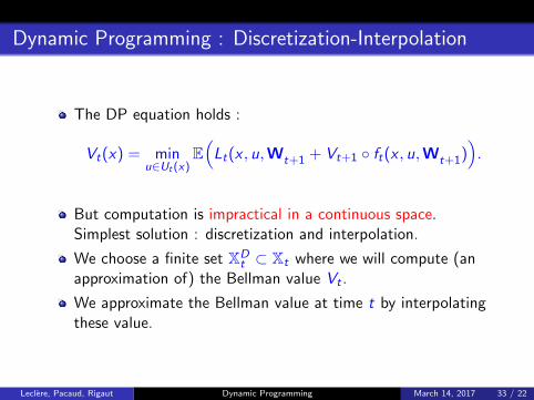
Dynamic Programming : Discretization-Interpolation
The DP equation holds :
Vt(x) = minu∈Ut(x)
E(
Lt(x , u,Wt+1 + Vt+1 ◦ ft(x , u,Wt+1)).
But computation is impractical in a continuous space.Simplest solution : discretization and interpolation.
We choose a finite set XDt ⊂ Xt where we will compute (an
approximation of) the Bellman value Vt .
We approximate the Bellman value at time t by interpolatingthese value.
Leclere, Pacaud, Rigaut Dynamic Programming March 14, 2017 33 / 22

Dynamic Programming : Discretization-Interpolation
Data: Problem parameters, discretization,one-stage solver, interpolation operator;
Result: approximation of optimal value;VT ≡ K ;for t : T − 1→ 0 do
for x ∈ XDt do
Vt(x) := minu∈Ut(x)
E(
Lt(x , u,Wt+1)+Vt+1◦ft(x , u,Wt+1
));
Define Vt by interpolating {Vt(x) | x ∈ XDt };
Algorithm 4: Dynamic Programming Algorithm (Continuous)
The strategy obtained is given by
πt(x) ∈ arg minu∈Ut(x)
E(
Lt(x , u,Wt+1) + Vt+1 ◦ ft(x , u,Wt+1
)).
Leclere, Pacaud, Rigaut Dynamic Programming March 14, 2017 34 / 22

Numerical considerations
The discrete case algorithm a look-up table of optimal controlfor every possible state offline.
In the continuous case we focus on computing offline anapproximation of the value function Vt and derive the optimalcontrol online by solving a one-step problem, solved only atthe current state :
πt(x) ∈ arg minu∈Ut(x)
E(
Lt(x , u,Wt+1) + Vt+1 ◦ ft(x , u,Wt+1
))
The field of Approximate DP gives methods for computingthose approximate value function (decomposed on a base offunctions).
The simpler one consisting in discretizing the state, and theninterpolating the value function.
Leclere, Pacaud, Rigaut Dynamic Programming March 14, 2017 35 / 22

Independence of noises
The Dynamic Programming equation requires only thetime-independence of noises.
This can be relaxed if we consider an extended state.
Consider a dynamic system driven by an equation
Yt+1 = ft(Yt ,Ut , εt+1)
where the random noise εt is an AR-1 process :
εt = αtεt−1 + βt + Wt ,
{Wt}t∈Z being independent.
Then Yt is called the physical state of the system and DP canbe used with the information state Xt = (Yt , εt).
Generically speaking, if the noise Wt is exogeneous (notaffected by decisions Ut), then we can always apply DynamicProgramming with the state (Xt ,W1, . . . ,Wt).
Leclere, Pacaud, Rigaut Dynamic Programming March 14, 2017 36 / 22


![Antony and Cleopatra [James F. Bellman, Kathryn Bellman]](https://img.pdfslide.us/doc/110x75/55cf9761550346d03391502a/antony-and-cleopatra-james-f-bellman-kathryn-bellman.jpg)