Stochastic Block Economic Value Modelling

R. Manjoo-Docrat1 Y. Bouchareb2 T. Motsepa3

T. Marote1 I. Denham-Dyson1

Supervisors: Montaz. Ali1

Industry Representative: Tinashe. Tholana

1University of the Witwatersrand2African institute for mathematical Sciences

3North West University

Mathematics in Industry Study Group, 2018

1 / 32

Introduction

Block Economic Value

Block Economic Value(BEV) = Block Revenue− Cost

BEVij = [(Tij ∗Gij ∗Rij ∗ Pt)− (MCt + PCt)]

2 / 32

Problem Description

Develop a model that accounts for the variability in the factorsused to calculate BEV

Block Economic Value

BEVij = [(Tij ∗Gij ∗Rij ∗ Pt)− (MCt + PCt)] (1)

where

Tij is the tonnage of block Bij ;

Gij is the grade of block Bij ;

Rij is the recovery of block Bij ;

Pt is the price of gold of the block Bij ;

MCt is the mining cost of block Bij at time t;

PCt is the cost of processing block Bij at time t.

3 / 32

Fitting Distributions for Parameters

Tonnage (Tij): Does not vary much between the observations:

Tij = t̄ =1

N

N∑i=1

Tij = 624.3

Recovery (Rij): Set as a constant as suggested by industry expert

Rij = r = 0.9

Cost of Mining (Ct): We model costs taking inflation intoconsideration

dC

dt= δC =⇒ Ct = C0e

δt

where

C(0) = C0 is the initial cost.

δ is the continuous inflation rate.

4 / 32

Visual representation of the dataGrade data

5 / 32

Visual representation of the dataPrice change

6 / 32

Visual representation of the dataPrice over time

7 / 32

Find possible models for the dataGrade

8 / 32

Parametric methodsWeibull distribution

9 / 32

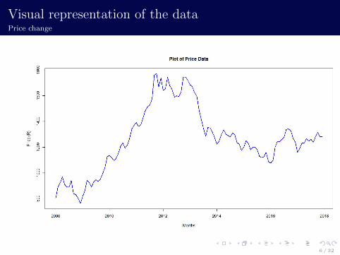
Parametric methodslog-normal distribution

10 / 32

Parametric methodsA comparison

11 / 32

Fitting Distributions for Parameters

Grade (Gij)We worked with gold data of 302 391 observations.We agree with that the lognormal is the best fits the data

f(g) =1

gσ√

2πexp

(− (ln g − µ)2

2σ2

)(2)

where

µ = −2.2366549 (0.001702716);σ = 0.9363237 (0.001203996).

12 / 32

Derivation of Stochastic process for Price of Gold

Define the ratio∆P

Ptwhere ∆P = Pt′ − Pt and ∆t = t′ − t

Expected annual increase:

µ∆t = E

[∆P

Pt

](3)

where µ is the increase per unit time.

Noise:

σ2∆t = V ar

(∆P

Pt

)(4)

where σ is the standard deviation.

13 / 32

Derivation of Stochastic process for Price of Gold

We can therefore construct a simple model.

∆P

Pt= µ∆t+ γ(σ) (5)

Where γ(σ) is the noise term.

To generate noise, we sample from a standard normaldistribution.

γ(σ) = σ√

∆tε, ε ∼ N(0, 1)

We must check that this satisfies the requirements of expectation andvariance for our model.

E[γ] = 0

V ar(γ) = σ2∆t

14 / 32

Derivation of Stochastic process for Price of Gold

So the model becomes,

∆P

Pt= µ∆t+ εσ

√∆t

Writing this as an SDE we have

dPt = Pt[µdt+ σdB(t)]

Where B(t) is standard Brownian Motion

We now let z = logPt and use Ito’s Lemma,

dFt = F ′(Xt)dXt +1

2F ′′(Xt)(dXt)

2

dz =1

PtdPt +

1

2

−1

P 2t

(dPt)2

15 / 32

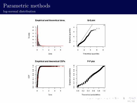
Derivation of Stochastic process for Price of Gold

Calculating these terms we have,

(dPt)2 = σ2P 2

t dt

Since dt2 = 0, dtdB(t) = 0 and dB(t)2 = dt. These fundamentalrelationships are known as quadratic variations.

So we arrive at,

dz =1

Pt(Pt[µdt+ σdB(t)])− 1

2P 2t

σ2P 2t dt

dz =

(µ− σ2

2

)dt+ σdB(t)

16 / 32

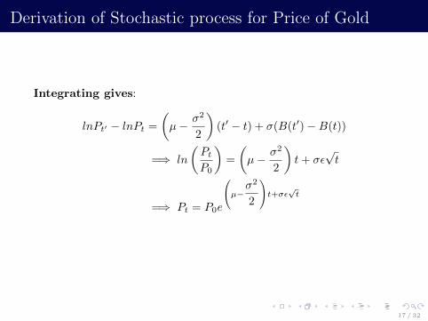
Derivation of Stochastic process for Price of Gold

Integrating gives:

lnPt′ − lnPt =

(µ− σ2

2

)(t′ − t) + σ(B(t′)−B(t))

=⇒ ln

(PtP0

)=

(µ− σ2

2

)t+ σε

√t

=⇒ Pt = P0e

µ−σ2

2

t+σε√t

17 / 32

Estimating volatility and drift

Volatility

Using 10 years of data sampled monthly we estimated thevolatility and drift of gold.Let P the list of all prices and ∆P their associated differences.

σ2 = Mean

(∆P 2

P 2dt

)= 0.0188871

18 / 32

Estimating volatility and drift

Drift

The log-rate is required in the calculation of the drift.

∆Pe∆t =PTP0

=⇒ log ∆P =log(PT )− log(P0)

∆T

=⇒ µ =σ2

2+ log ∆P

= 0.13743

19 / 32

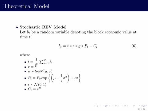
Theoretical Model

Stochastic BEV ModelLet bt be a random variable denoting the block economic value attime t

bt = t ∗ r ∗ g ∗ Pt − Ct (6)

where

t =1

N

∑Nn=1 ti

r = r̄g ∼ logN (µ, σ)

Pt = P0 exp

{(µ− 1

2σ2

)+ εσ

}ε ∼ N (0, 1)Ct = eδt

20 / 32

Conditional distribution

Conditional Stochastic BEV ModelTo calculate the BEV, we define the following conditionaldistribution:

f(bt|g) = P (bt < x|α < g < β) (7)

Applying Baye’s Theorem

f(bt|g) =P (bt < x ∩ α < g < β)

P (α < g < β)(8)

Taking the expectation yields the Block Economic Value at aparticular grade

21 / 32

Implementing the model

Conditional ProbabilitySuppose the mining company wishes to determine the probabilitythat a block value will be above x dollars if the grade is between0.5ppm and 1ppm i.e Pr(BEV > x|1 > g > 0.5).

x Dollars Probability1000 0.8377392000 0.6006093000 0.4306344000 0.3154985000 0.2364926000 0.1809697000 0.1410018000 0.1115969000 0.089539710000 0.0727107

22 / 32

Implementing the model

Conditional ExpectationThis may be useful for various forms of statistical analysis butthe company may want a more direct means of evaluatingpotential prospects.

Grade Expected BEV(0.1,0.2) 3398.79(0.2,0.3) 5823.56(0.3,0.4) 8246.05(0.4,0.5) 10662.8(0.5,0.6) 13075.5(0.6,0.7) 15485.4

23 / 32

Implementing the model

Time averagesThe time average is given by

1

T

∫ T

0

f(t)dt

Take the time average of P (t).Generate several values of the now time independent PT .Form a distribution over these values.Take the time average of C(t).Substitute these into the model and generate several values.Plot the BEV against g

24 / 32

0.1 0.2 0.3 0.4 0.5

2000

4000

6000

8000

10000

12000

25 / 32

26 / 32

27 / 32

28 / 32

29 / 32

Conclusion

Our model incorporates two tools parameter fitting and stockmodelling.

Incorporate kriging

30 / 32

References

Chance, Don M. ”The ABCs of Geometric Brownian Motion.”Derivatives Quarterly 41 (1994).

31 / 32

32 / 32