This article was downloaded by: [University of Nebraska, Lincoln]On: 17 October 2014, At: 09:55Publisher: Taylor & FrancisInforma Ltd Registered in England and Wales Registered Number: 1072954Registered office: Mortimer House, 37-41 Mortimer Street, London W1T 3JH,UK

Stochastic Analysis andApplicationsPublication details, including instructions forauthors and subscription information:http://www.tandfonline.com/loi/lsaa20

Stochastic ApproximationAlgorithms for ParameterEstimation in Option Pricingwith Regime SwitchingG. Yin a , Q. Zhang b & C. Zhuang ba Department of Mathematics , Wayne StateUniversity , Detroit, Michigan, USAb Department of Mathematics , University ofGeorgia , Athens, Georgia, USAPublished online: 30 Oct 2007.

To cite this article: G. Yin , Q. Zhang & C. Zhuang (2007) StochasticApproximation Algorithms for Parameter Estimation in Option Pricing withRegime Switching, Stochastic Analysis and Applications, 25:6, 1243-1261, DOI:10.1080/07362990701567322

To link to this article: http://dx.doi.org/10.1080/07362990701567322

PLEASE SCROLL DOWN FOR ARTICLE

Taylor & Francis makes every effort to ensure the accuracy of all theinformation (the “Content”) contained in the publications on our platform.However, Taylor & Francis, our agents, and our licensors make norepresentations or warranties whatsoever as to the accuracy, completeness,or suitability for any purpose of the Content. Any opinions and viewsexpressed in this publication are the opinions and views of the authors, andare not the views of or endorsed by Taylor & Francis. The accuracy of theContent should not be relied upon and should be independently verified withprimary sources of information. Taylor and Francis shall not be liable for anylosses, actions, claims, proceedings, demands, costs, expenses, damages,

and other liabilities whatsoever or howsoever caused arising directly orindirectly in connection with, in relation to or arising out of the use of theContent.

This article may be used for research, teaching, and private study purposes.Any substantial or systematic reproduction, redistribution, reselling, loan,sub-licensing, systematic supply, or distribution in any form to anyone isexpressly forbidden. Terms & Conditions of access and use can be found athttp://www.tandfonline.com/page/terms-and-conditions

Dow

nloa

ded

by [

Uni

vers

ity o

f N

ebra

ska,

Lin

coln

] at

09:

55 1

7 O

ctob

er 2

014

Stochastic Analysis and Applications, 25: 1243–1261, 2007Copyright © Taylor & Francis Group, LLCISSN 0736-2994 print/1532-9356 onlineDOI: 10.1080/07362990701567322

Stochastic Approximation Algorithms for ParameterEstimation in Option Pricing with Regime Switching

G. YinDepartment of Mathematics, Wayne State University,

Detroit, Michigan, USA

Q. Zhang and C. ZhuangDepartment of Mathematics, University of Georgia,

Athens, Georgia, USA

Abstract: This work is concerned with option pricing. Stochasticapproximation/optimization algorithms are proposed and analyzed. Theunderlying stock price evolves according to two geometric Brownian motionscoupled by a continuous-time finite state Markov chain. Recursive stochasticapproximation algorithms are developed to estimate the implied volatility.Convergence of the algorithm is proved. Rate of convergence is also ascertained.Then real market data are used to compare our algorithms with other schemes.

Keywords: Option pricing; Parameter estimation; Stochastic approximation.

Mathematics Subject Classification: 62L20; 91B28.

1. INTRODUCTION

This work is concerned with parameter estimations in option pricing.In the finance literature, the celebrated Black-Scholes model is widely

Received October 10, 2006; Accepted March 1, 2007We are very grateful to Dr. Reza Kamaly and Necessity and Chance LLC for

providing us with data derived from Berkeley Options Data Base. This researchwas supported in part by the National Science Foundation.

Address correspondence to George Yin, Department of Mathematics, WayneState University, Detroit, MI 48202, USA; E-mail: gyin@math.wayne.edu

Dow

nloa

ded

by [

Uni

vers

ity o

f N

ebra

ska,

Lin

coln

] at

09:

55 1

7 O

ctob

er 2

014

1244 Yin et al.

used in analysis of option and portfolio management. Traditionally ageometric Brownian motion (GBM) is used to capture the dynamicsof the stock market by using a stochastic differential equation witha deterministic expected return and a nonrandom volatility. It givesa reasonably good description of the market in a short time period.However, in the long run, it fails to describe the behavior of the stockprice. This is mainly due to insensitivity to random parameter changes.In fact, it is well understood that the stock prices are far away frombeing a “random walk” in a longer time horizon. Recognizing the needs,various modifications of the models have been made. One of the ideasis to use a secondary stochastic differential equation to model thestochastic volatility.

One of the main factors that affects the option prices in a market-place is the trend of the volatility. It is necessary to incorporate suchtrends in modeling to capture detailed stock price movements. In a recentarticle of Zhang [10], a hybrid switching GBMmodel, involving a numberof GBMs modulated by a finite-state Markov chain, is proposed. Suchswitching processes can be used to represent market trends or the trends ofan individual stock.

The above switching GBM model has been used in Yao et al. [8] forpricing European options; a closed-form solution is obtained assumingthe underlying Markov chain jumps only once. To use the result inpractice, it is necessary to estimate various parameters. To accomplishthis, it is natural to use market option prices to carry out estimationtasks. One of the parameters to be estimated is the implied volatility.Normally, a large number of observations are needed to derive ameaningful estimator of the parameter. More observations typicallybring better estimates. On the other hand, using more observations willtake longer time to reach the desired result. Thus, the time needed forsuccessfully estimating the parameter is a major concern in applications.

A standard approach is to use the least squares method, which givesa benchmark for comparison purposes. However, in view of real-timetrading, the least squares method is too slow to meet the practical needs.In this article, we aim to find an alternative feasible algorithm thatcan be easily implemented for pricing options in real time. Inspired bythe approach initiated in Yin et al. [9] for treating stock liquidation,we develop stochastic approximation algorithms to estimate impliedvolatility first. Then we use the estimated parameter to price options.

The rest of the article is arranged as follows. Section 2 begins withthe precise formulation of the problem. The model is given and then therecursive algorithm is proposed. The advantages include the simple formand systematic nature of the algorithms. In particular, it is useful foronline computation. Another nice feature of the proposed algorithm isthat only a few observations are needed. Section 3 then proceeds withthe study of the asymptotic properties of the underlying algorithm; the

Dow

nloa

ded

by [

Uni

vers

ity o

f N

ebra

ska,

Lin

coln

] at

09:

55 1

7 O

ctob

er 2

014

Stochastic Approximation for Option 1245

convergence of the algorithm is obtained. The rate of convergence isascertained in Section 4. To demonstrate the feasibility and efficiency ofthe algorithms, numerical experiments using real market data are givenin Section 5. The experiments indicate the stochastic approximationalgorithms indeed provide good estimates of the desired parameter witha reasonably fast convergence speed and predict more accurately theoption price than that of the traditional Black–Scholes model. Finally,we close the paper with some further remarks in Section 6.

2. FORMULATION

2.1. Hybrid GBM Model

In a regime-switching model, one typically uses a finite-state Markovchain ��·� = ���t� � t ≥ 0� to capture changes in the rate of return andthe volatility of a stock to reflect the market modes. Let X�t� denote theprice of the stock at time t, which is governed by the following stochasticdifferential equation,

dX�t� = X�t������t��dt + ���t��dw�t�� 0 ≤ t ≤ T� (2.1)

where X�0� = X0 is the initial stock price at t = 0; ��i� and �i� for eachi ∈ � with � = �1� 2�, represent the expected rate of return and volatilityof the stock price at regime i; w�·� is a standard one-dimensionalBrownian motion independent of the Markov chain ��·�.

In this article, we consider the case that the Markov chain jumpsat most once on �0� T. The corresponding generator is Q = ( −� �

0 0

). That

is, state 2 is an absorbing state. If we take ��0� = 1, then there exits astopping time such that is exponentially distributed with parameter �and

��t� ={1� if t < �

2� if t ≥ �(2.2)

Therefore, the volatility process ���t�� jumps at most once attime t = . Its jump size is ��2�− �1��, and the average sojourn timein state 1 (before jumping to state 2) is 1/�. A closed-form solutionfor European call option price has been obtained in Yao et al. [8].In practice, we may already know the market prices for some options.Thus, we may assume that �1� is the implied volatility given by Black–Scholes model and � is a known constant. We need only estimate thevalue of �2� to calculate the price of a call option. Our goal here isto estimate the true value of �2� given some real option prices. Forconvenience, we use instead of �2� throughout the rest of the articleif there is no confusion.

Dow

nloa

ded

by [

Uni

vers

ity o

f N

ebra

ska,

Lin

coln

] at

09:

55 1

7 O

ctob

er 2

014

1246 Yin et al.

2.2. Stochastic Recursive Algorithm

In what follows, we formulate the task of finding the optimal value of as a stochastic optimization problem. We aim to find the optimal value ∈ �0��� so that a suitable objective function (the expected error) isminimized. The problem can be written as:

Problem � � Find argmin ��� = E�c��− cn2/2� ∈ �0���� (2.3)

where c�� is the option price using model (2.1) and cn is thecorresponding market price observed at time n.

To obtain the desired estimate, we construct a recursive procedure

n+1 = �[n − �n�c�n�− cnc�n�

]� (2.4)

where ��n� is a sequence of nonnegative decreasing step sizes satisfying�n → 0 as n → �, and

∑n �n = �, c�·� denotes the derivative of c�·�,

and � = ��0�M for some M > 0 is a projection operator given by

�� =

0� if < 0�

M� if > M�

� otherwise.

We have used a projection device to make sure that the estimates arenonnegative. Moreover, we choose M to be a sufficiently large number sothe estimate of the volatility stays bounded. As explained in Kushner andYin [7], the projection algorithm may be written in an expanded form as

n+1 = n − �n�c�n�− cnc�n�+ �nRn� (2.5)

where �nRn = n+1 − n + �n�c�n�− cnc�n� is the real number withthe shortest distance needed to bring n − �n�c�n�− cnc�n� back tothe interval �0�M if it ever escapes from there.

3. CONVERGENCE

We proceed to prove the convergence of the algorithm. For simplicity,the step size ��n� is assumed to be of the form �n = O�1/n� henceforth.We will show that n defined in (2.4) is closely related to an ordinarydifferential equation. First, let us state a couple of conditions needed inwhat follows.

(A1) The derivative c�·� is continuous.

Dow

nloa

ded

by [

Uni

vers

ity o

f N

ebra

ska,

Lin

coln

] at

09:

55 1

7 O

ctob

er 2

014

Stochastic Approximation for Option 1247

(A2) There is a c such that

�n

n−1∑k=0

ck → c w.p.1 as n → �� (3.1)

Remark 3.1. Our objective here is to minimize the function ��� givenin (2.3). Condition (A1) is satisfied in the context of typical optionproblems. Next we show that (A1) is satisfied in the case that the Markovchain has only two states for the European call option. In particular,we show that for the European option c�� is twice continuouslydifferentiable. As in Yao et al. [8], given the risk-free rate r, the currentstock price x, the maturity T , the strike price K, and the volatility vector�0� � ��, the call option price can be given as follows. Suppose that theMarkov chain initially takes the value ��0� = 1. Then

c�� = x∫ T

0e−rT

(∫ �

−�eu�0�t� u+ log x� 2���u� �r − 0/2�t� 0t�du

)�e−�t dt

+ xe−�T�0�0� log x� 1�� (3.2)

where

�0�s� y� 1� = e−y−r�T−s�∫ �

−�h�ey+u���u� �r − 0/2��T − s�� 0�T − s��du�

�0�s� y� 2� = e−y−r�T−s�∫ �

−�h�ey+u���u� �r − /2��T − s�� �T − s��du�

��u�m��� is the Gaussian density function with mean m and variance �,

h�x� = �x − K�+�

It is then easy to see the twice continuously differentiability of c�� withrespect to .

Condition (A2) is essentially a law of large numbers condition.Take for instance, �n = 1/n. Then it is precisely the usual ergodicity ofthe sequence �cn�. Suppose that �cn� is a stationary �-mixing sequence.Then it is strongly ergodic. In such a case, (3.1) is readily verified.

To analyze the algorithm, we take a piecewise constant interpolationand work with a sequence of functions instead of the discrete iterates.To this end, define

t0 = 0� tn =n−1∑k=0

�k�

m�t� ={n� tn ≤ t < tn+1� for t ≥ 0�

0� for t < 0�

Dow

nloa

ded

by [

Uni

vers

ity o

f N

ebra

ska,

Lin

coln

] at

09:

55 1

7 O

ctob

er 2

014

1248 Yin et al.

Define the continuous time interpolation 0�·� on �−���� by

0�t� ={0� for t < 0�

n for t ≥ 0 and tn ≤ t < tn+1�

Define a shifted process n�·� byn�t� = 0�tn + t�� t ∈ �−�����

Moreover, define

Rn = 0 and �c�n�− cnc�n� = 0� for n < 0�

R0�t� =m�t�−1∑k=0

�kRk for t ≥ 0�

Rn�t� =

R0�tn + t�− R0�tn� =

m�tn+t�−1∑k=n

�kRk� t ≥ 0�

−n−1∑

k=m�tn+t�

�kRk� t < 0�

As in Kushner and Yin [7] (Section 4.3), define a set C�� as follows.For ∈ �0�M�, C�� contains only the zero element; for = 0 or =M , C�� is the infinite cone (interval �−�� 0� or �M���) pointing to thedirection away from �0�M.

Theorem 3.2. Assume conditions (A1) and (A2). Then w.p.1, �n�·�� Rn�·��is equicontinuous in the extended sense (see Kushner and Yin [7] (p. 102)).Let ��·�� R�·�� be the limit of a convergent subsequence of �n�·�� Rn�·��(still indexed by n for simplicity). Then it satisfies the projected ordinarydifferential equation

�t� = −�c��t��− cc��t��+ r�t�� r�t� ∈ −C��t��� (3.3)

where r is the minimal force needed to keep the solution in �0�M with

R�t� =∫ t

0r�s�ds�

Proof. Note that (2.5) can be written as

n+1 = n − �n�c�n�c�n�− cc�n�+ �n�cn − c�c�n�+ �nRn� (3.4)

Define

cn = −�c�n�− cc�n�� for n ≥ 0� and cn = 0 for n < 0�

cn = �cn − cc�n� for n ≥ 0� and cn = 0 for n < 0�

Dow

nloa

ded

by [

Uni

vers

ity o

f N

ebra

ska,

Lin

coln

] at

09:

55 1

7 O

ctob

er 2

014

Stochastic Approximation for Option 1249

Define the interpolations of cn and cn as c0�·�, cn�·�, c0�·�, and cn�·�similar to that of R0�·� and Rn�·�. Then

n�t� = n + cn�t�+ cn�t�� for t ∈ �−�����

To proceed, we use Kushner and Yin [7], (Theorem 6.1.1) to provethe theorem. In this process, we need only verify an asymptotic rate ofchange condition holds. For each , define

��t�def=

m�t�−1∑k=0

�k�ck − c�c���

Recall that the asymptotic rate of change of ��t� is said to go to 0 withprobability 1 if for some T > 0,

limn

supj≥n

max0≤t≤T

���jT + t�−��jT�� = 0 w.p.1.

To proceed, define

Dn

def=n∑

k=0

�ck − c�

Note that by means of a partial summation,

n∑k=m

�k�ck − cc��= �n�Dn+1 −Dmc��+n−1∑k=m

�Dk+1 −Dm��k − �k+1c���

Taking m = 0, n = m�t�− 1, we obtain

��t� = �m�t�−1Dm�t�c��+m�t�−2∑k=0

Dk+1�k − �k+1

�k

�kc���

Note that (A2) implies that �m�t�−1Dm�t�c�� → 0 as m�t� → �(or n→�) and

m�t�−2∑k=0

Dk+1�k − �k+1

�k

�kc�� =m�t�−2∑k=0

Dk+1O��2k�c�� → 0�

Thus, the asymptotic rate of changes of ��t� goes to 0 w.p.1. By usingKushner and Yin [7], (Theorem 6.1.1) the desired result then follows. �

Corollary 3.3. In addition to the conditions in Theorem 3.2, suppose thatc�� �= 0 for all , and that ∗ is the unique solution of c��− c = 0 with∗ ∈ �0�M� such that ∗ is in the set of locally asymptotic stable points ofthe projected ODE. Then n → ∗ w.p.1.

Dow

nloa

ded

by [

Uni

vers

ity o

f N

ebra

ska,

Lin

coln

] at

09:

55 1

7 O

ctob

er 2

014

1250 Yin et al.

Remark 3.4. In view of the definition of the cost function, ∗ is the uniqueminimizer of � defined in (2.3). Thus, the result indicates that the algorithmthat we constructed converges to the unique minimizer of the least squarescost function.

Proof. We merely indicate that by use of the asymptotic stability in thesense of Liapunov (see Kushner and Yin [7] (p. 104)), for any sn → �as n → �, using the argument as in Theorem 3.2, n�· + sn� → ∗ w.p.1.

�

4. RATE OF CONVERGENCE

This section is devoted to the rate of convergence of algorithm (2.4).To further simplicity the matters, we take �n = 1/�n+ 1�. We assumethat all the conditions of Corollary 3.3 hold. Since ∗ is strictly interiorto the constrained set �0�M, without loss of generality, we will dropthe reflection term �nRn throughout this section, and assume that thesequence of iterates �n� is nonnegative and uniformly bounded by M .

Define un =√n+ 1�n − ∗�. The rate of convergence study aims to

exploit the asymptotic properties of this scaled sequence. We shall showthat the interpolation of un converges to a diffusion limit. One of the keypoints here is to use linearization and local analysis. First note that from(2.5) with the reflection term dropped, we can write

un+1 =√n+ 2n+ 1

un −1

n+ 1

√n+ 2n+ 1

c2�∗�un

+√n+ 2n+ 1

1√n+ 1

�cn − c�c�∗�+√n+ 2n+ 1

1n+ 1

�cn − c�g�un�

+ 1n+ 1

o��un��� (4.1)

where g�·� is a continuous function and g�u� = O��u��. Since√n+ 2n+ 1

= 1+ 12�n+ 1�

+ O

(1

�n+ 1�2

)� (4.2)

to study the asymptotics of un, we need only consider an auxiliaryprocess vn defined by

v0 = u0�

vn+1 = vn −1

n+ 1

(c2�∗�−

12

)vn +

1√n+ 1

�cn − c�c�∗� (4.3)

+ 1n+ 1

�cn − c�g�vn�+1

n+ 1o��vn���

Dow

nloa

ded

by [

Uni

vers

ity o

f N

ebra

ska,

Lin

coln

] at

09:

55 1

7 O

ctob

er 2

014

Stochastic Approximation for Option 1251

(A3) The �cn − c� is a stationary �-mixing sequence with 0 meanand mixing rate �k satisfying

∑�k=0 �

1/2k < �. In addition, suppose

c2�∗� > 1/2.

Remark 4.1. Under (A3), it can be shown (see Kushner and Yin [7](Chapter 7)) that

∑m�t�−1k=0

1√k+1

�ck − c� converges weakly to a real-valuedstandard Brownian motion with variance �2t� where

�2 = E�c0 − c�2 + 2�∑k=1

E�ck − c��c0 − c��

Moreover, by using the well-known mixing inequality (see [1] (p. 166)),we obtain

E

∣∣∣∣ n−1∑k=0

1√k+ 1

�ck − c�

∣∣∣∣2 ≤ K

for some K > 0.

Lemma 4.2. In addition to the conditions of Corollary 3.3, assume (A3)holds. Then �vn� is tight.

Proof. We claim that supn E�vn� < �� To this end, define

Ank =

n∏

j=k+1

(1− c2�∗�− 1

2

j + 1

)� if k < n�

1� if k = n�

Then

vn+1 = An0v0 +

n∑k=0

1√k+ 1

Ank�ck − c�c�∗�

+n∑

k=0

1k+ 1

Ank�ck − c�g�vk�+n∑

k=0

1k+ 1

Anko��vk���

Note that in view of (A3), E�ck − c��g�vk�� ≤ KE�vk�. Thus, we obtain

E�vn+1� ≤ �An0�E�v0� + E

∣∣∣∣ n∑k=0

1√k+ 1

Ank�ck − c�c�∗�∣∣∣∣

+ Kn∑

k=0

1k+ 1

�Ank�E�vk�� (4.4)

It is easily verified that by (A3),

n∑k=0

1k+ 1

�Ank� =n∑

k=0

1k+ 1

Ank < ��

Dow

nloa

ded

by [

Uni

vers

ity o

f N

ebra

ska,

Lin

coln

] at

09:

55 1

7 O

ctob

er 2

014

1252 Yin et al.

Using the mixing inequality [1], we have

E

∣∣∣∣ n∑k=0

1√k+ 1

Ank�ck − c�c�∗�∣∣∣∣

≤ E12

∣∣∣∣ n∑k=0

1√k+ 1

Ank�ck − c�c�∗�∣∣∣∣2

=( n∑

k=0

n∑j=0

1√k+ 1

1√j + 1

AnkAnjE�ck − c��cj − c�c2�∗�) 1

2

≤ K

( n∑j=0

1j + 1

A2nj

n∑k>j

E�ck − c��cj − c�c2�∗�) 1

2

≤ K

( n∑j=0

1j + 1

A2nj

n∑k>j

�E�ck − c��cj − c�− E�ck − c�E�cj − c��) 1

2

≤ K

( n∑j=0

1j + 1

A2nj

n∑k<j

�k−j

) 12

≤ K < ��

Recall that we use K as a generic positive constant, whose value maychange for different appearances. Combining the above estimates, wearrive at

E�vn+1� ≤ K + Kn∑

k=0

1k+ 1

�Ank�E�vk�� (4.5)

An application of the Gronwall’s inequality leads to

E�vn+1� ≤ K < � and supn

E�vn� < ��

The desired tightness then follows from the well-knownMarkov inequality

P(�vn� ≥ K

) ≤ supn E�vn�K

�

The lemma is proved. �

Lemma 4.3. Under the conditions of Lemma 4.2, limn E�vn − un� = 0.

Proof. We merely use the expansions in (4.2), and the definitions ofun and vn in (4.1) and (4.3), respectively. Detailed calculation yields thedesired result. �

Dow

nloa

ded

by [

Uni

vers

ity o

f N

ebra

ska,

Lin

coln

] at

09:

55 1

7 O

ctob

er 2

014

Stochastic Approximation for Option 1253

Consider the sequence �vn�. Define a piecewise constant inter-polation v0�t� and its shift vn�t� as in the previous section. We then have

vn�t + s�− vn�t�

=m�tn+t+s�−1∑j=m�tn+t�

1j + 1

(c2�∗�−

12

)vj +

m�tn+t+s�−1∑j=m�tn+t�

1√j + 1

�cj − c�c�∗�

+m�tn+t+s�−1∑j=m�tn+t�

1j + 1

�cj − c�g�vj�+m�tn+t+s�−1∑j=m�tn+t�

1j + 1

hjvj� (4.6)

Our next result shows that the scaled sequence vn�·� converges weakly tov�·�, a diffusion process.

Theorem 4.4. The sequence of interpolated estimation errors �vn�·�� conver-ges weakly to v�·�, which is a solution of the stochastic differential equation

dv =(c2�∗�−

12

)v dt + �c�∗�dw� (4.7)

where w�·� is a real-valued standard Brownian motion.

Proof. The proof is naturally divided into two steps. The first step estab-lishes the tightness, whereas the second step characterizes the limit process.

Step 1) Show that the sequence �vn�·�� is tight in D�0��� thespace of functions that are right continuous, have left limits, endowedwith the Skorohod topology. To this end, we apply the tightnesscriterion in Kushner and Yin [7]. Without loss of generality and fornotational simplicity, assume that �vn� is bounded (otherwise, we can usea truncation device as in [7]).

Then we obtain that for any t > 0, � > 0, and any 0 < s ≤ �,

E�vn�t + s�− vn�t��2 ≤ I1 + I2 + I3 + I4� (4.8)

where Ii for i = 1� 2� 3� 4 are four terms on the right-hand side of (4.6).By virtue of the boundedness of �vk�,

I1 = E

∣∣∣∣ m�tn+t+s�−1∑j=m�tn+t�

1j + 1

(c2�∗�−

12

)vj

∣∣∣∣2

≤ Km�tn+t+s�−1∑j=m�tn+t�

m�tn+t+s�−1∑k=m�tn+t�

1j + 1

1k+ 1

≤ Ks2 ≤ K�2� (4.9)

Thus, taking lim supn followed by lim�→0, the limit is 0.

Dow

nloa

ded

by [

Uni

vers

ity o

f N

ebra

ska,

Lin

coln

] at

09:

55 1

7 O

ctob

er 2

014

1254 Yin et al.

The mixing inequality implies that

I2 = E

∣∣∣∣ m�tn+t+s�−1∑j=m�tn+t�

1√j + 1

�cj − c�c�∗�∣∣∣∣2

≤ Ks ≤ K�� (4.10)

Thus, the double limits of this term also goes to 0. Likewise,

I3 + I4 ≤ E

∣∣∣∣ m�tn+t+s�−1∑j=m�tn+t�

1√j + 1

�cj − c�g�vj�

∣∣∣∣2 + E

∣∣∣∣ m�tn+t+s�−1∑j=m�tn+t�

1√j + 1

hjvj

∣∣∣∣2≤ K�� (4.11)

Combining the estimates above, we arrive at

lim�→0

lim supn

E�vn�t + s�− vn�t��2 = 0� (4.12)

Therefore, �vn�·�� is tight.Step 2) Characterization of the limit process. By Prohorov’s

theorem, we can extract a convergent subsequence and still denote itby �vn�·�� for notational simplicity. Denote the limit by v�·�. By theSkorohod representation, without changing notation, we may assumethat the sequence vn�·� converges to v�·� w.p.1 and the convergence isuniform in any bounded time interval. We proceed to establish that thelimit is nothing but the desired diffusion process.

We shall show that v�·� is a solution of the martingale problem withoperator

�f�v� = 12�2c2�∗�

d2f�v�

dv2+

(c2�∗�−

12

)vdf�v�

dv� (4.13)

where f�·� is a C2 function with compact support. To this end, we showthat

f�v�t + s��− f�v�t��−∫ t+s

t�f�v� ��d is a martingale.

To do so, for any bounded and continuous function ��·�, any t� s > 0,any positive integer �, and 0 ≤ t1 ≤ t2 ≤ · · · ≤ t� ≤ t, we will show

E��v�ti� � i ≤ ��

[f�v�t + s��− f�v�t��−

∫ t+s

t�f�v� ��d

]= 0�

Dow

nloa

ded

by [

Uni

vers

ity o

f N

ebra

ska,

Lin

coln

] at

09:

55 1

7 O

ctob

er 2

014

Stochastic Approximation for Option 1255

First, by the weak convergence and the Skorohod representation, it isreadily seen that

E��vn�ti� � i ≤ ���f�vn�t + s��− f�vn�t��

→ ��v�ti� � i ≤ ���f�v�t + s��− f�v�t�� as n → �� (4.14)

Let �n be a sequence a positive real numbers satisfying �n → 0and select an increasing sequence �m��n�� such that m�tn + t� = m1�n� <

m2�n� < · · · ≤ m�tn + t + s�− 1, and that for m�tn + t� ≤ m� ≤ m�+1 ≤m�tn + t + s�− 1�

1�n

m�+1�n�−1∑j=m��n�

1j + 1

→ 1 as n → ��

In what follows, for notational simplicity, we suppress the n dependencein m��n� and write it as m� instead. Denote by Im the index set satisfyingm�tn + t� ≤ m� ≤ m�+1 ≤ m�tn + t + s�− 1. Using the notation definedabove, we have

f�vn�t + s��− f�vn�t��

= ∑�∈Im

�f�vm�+1�− f�vm�

� = ∑�∈Im

df�vm��

dv

[ m�+1−1∑j=m�

�vj+1 − vj�

]

+ ∑�∈Im

12

d2f�vm��

dv2

[ m�+1−1∑j=m�

�vj+1 − vj�

]2

+ o�1�� (4.15)

where o�1� → 0 in probability uniformly in t.It follows that

E��vn�ti� � i ≤ ��∑�∈Im

df�vm��

dv

[ m�+1−1∑j=m�

�vj+1 − vj�

]

= E��vn�ti� � i ≤ ��∑�∈Im

df�vm��

dvEm�

×[−

m�+1−1∑j=m�

1j + 1

(c2�∗�−

12

)vj +

m�+1−1∑j=m�

1√j + 1

�cj − c�c�∗�

+m�+1−1∑j=m�

1j + 1

�cj − c�g�vj�+m�+1−1∑j=m�

1j + 1

hjvj

]� (4.16)

Dow

nloa

ded

by [

Uni

vers

ity o

f N

ebra

ska,

Lin

coln

] at

09:

55 1

7 O

ctob

er 2

014

1256 Yin et al.

Then

limn

E��vn�ti� � i ≤ ��∑�∈Im

df�vm��

dv

[−

m�+1−1∑j=m�

1j + 1

(c2�∗�−

12

)vj

]

= limn

E��vn�ti� � i ≤ ��∑�∈Im

df�vm��

dv

[−

m�+1−1∑j=m�

1j + 1

(c2�∗�−

12

)vm�

]

= E��v�ti� � i ≤ ��

[−

∫ t+s

t

df�v� ��

d

(c2�∗�−

12

)v� �d

]� (4.17)

As for the next term, using the mixing property,

limn

E��vn�ti� � i ≤ ��∑�∈Im

df�vm��

dv

[−

m�+1−1∑j=m�

1√j + 1

�cj − c�c�∗�]

= limn

E��vn�ti� � i ≤ ��∑�∈Im

df�vm��

dv

×[−

m�+1−1∑j=m�

1√j + 1

Em��cj − c�c�∗�

]= 0� (4.18)

Using the continuity of g�·�, detailed calculation also shows that

limn

E��vn�ti� � i ≤ ��∑�∈Im

df�vm��

dv

[ m�+1−1∑j=m�

1j + 1

�cj − c�g�vj�

]= 0�

limn

E��vn�ti� � i ≤ ��∑�∈Im

df�vm��

dv

[ m�+1−1∑j=m�

1j + 1

hjvj

]= 0� (4.19)

Likewise, similar estimates lead to

limn

E��vn�ti� � i ≤ ��∑�∈Im

12

d2f�vm��

dv2

[ m�+1−1∑j=m�

�vj+1 − vj�

]2

= E��v�ti� � i ≤ ��

[12

∫ t+s

t

d2f�v� ��

dv2�2c2�∗�d

]� (4.20)

we omit the details for brevity. Thus, the desired result follows. �

Remark 4.5. Likewise, we can also construct an SA algorithm using aconstant step size

n+1 = ��n − ��c�n�− cnc�n�� (4.21)

Convergence of corresponding algorithm can also be obtained.

Dow

nloa

ded

by [

Uni

vers

ity o

f N

ebra

ska,

Lin

coln

] at

09:

55 1

7 O

ctob

er 2

014

Stochastic Approximation for Option 1257

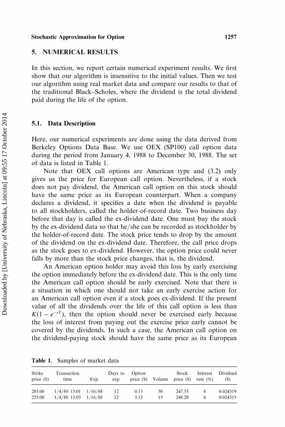
5. NUMERICAL RESULTS

In this section, we report certain numerical experiment results. We firstshow that our algorithm is insensitive to the initial values. Then we testour algorithm using real market data and compare our results to that ofthe traditional Black–Scholes, where the dividend is the total dividendpaid during the life of the option.

5.1. Data Description

Here, our numerical experiments are done using the data derived fromBerkeley Options Data Base. We use OEX (SP100) call option dataduring the period from January 4, 1988 to December 30, 1988. The setof data is listed in Table 1.

Note that OEX call options are American type and (3.2) onlygives us the price for European call option. Nevertheless, if a stockdoes not pay dividend, the American call option on this stock shouldhave the same price as its European counterpart. When a companydeclares a dividend, it specifies a date when the dividend is payableto all stockholders, called the holder-of-record date. Two business daybefore that day is called the ex-dividend date. One must buy the stockby the ex-dividend data so that he/she can be recorded as stockholder bythe holder-of-record date. The stock price tends to drop by the amountof the dividend on the ex-dividend date. Therefore, the call price dropsas the stock goes to ex-dividend. However, the option price could neverfalls by more than the stock price changes, that is, the dividend.

An American option holder may avoid this loss by early exercisingthe option immediately before the ex-dividend date. This is the only timethe American call option should be early exercised. Note that there isa situation in which one should not take an early exercise action foran American call option even if a stock goes ex-dividend. If the presentvalue of all the dividends over the life of this call option is less thanK�1− e−rT �, then the option should never be exercised early becausethe loss of interest from paying out the exercise price early cannot becovered by the dividends. In such a case, the American call option onthe dividend-paying stock should have the same price as its European

Table 1. Samples of market data

Strike Transaction Days to Option Stock Interest Dividendprice ($) time Exp. exp. price ($) Volume price ($) rate (%) ($)

285.00 1/4/88 13:01 1/16/88 12 0.13 50 247.55 6 0.024319255.00 1/4/88 13:03 1/16/88 12 3.13 15 248.20 6 0.024315

Dow

nloa

ded

by [

Uni

vers

ity o

f N

ebra

ska,

Lin

coln

] at

09:

55 1

7 O

ctob

er 2

014

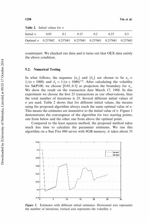
1258 Yin et al.

Table 2. Initial values for

Initial 0.05 0.1 0.15 0.2 0.25 0.3

Optimal 0.237682 0.237681 0.237681 0.237681 0.237681 0.237681

counterpart. We checked our data and it turns out that OEX data satisfythe above condition.

5.2. Numerical Testing

In what follows, the sequence ��n� and ��n� are chosen to be �n =1/�n+ 1000� and �n = 1/�n+ 1000�1/6. After calculating the volatilityfor S&P100, we choose �0�05� 0�5 as projection the boundary for n.We show the result on the transaction date March 17, 1988. In thisexperiment we choose the first 25 transactions as our observations, thusthe total number of iterations is 25. Several different initial values of are used. Table 2 shows that for different initial values, the iteratesusing the proposed algorithm always reach the same optimal value of .This means the estimates are insensitive to the initial value of . Figure 1demonstrates the convergence of the algorithm for two starting points,one from below and the other one from above the optimal point.

Compared to the least squares method, the proposed method takesmuch less time to calculate the parameter estimates. We run thisalgorithm on a Sun Fire 880 server with 8GB memory, it takes about 35

Figure 1. Estimates with different initial estimates. Horizontal axis representsthe number of iterations; vertical axis represents the volatility .

Dow

nloa

ded

by [

Uni

vers

ity o

f N

ebra

ska,

Lin

coln

] at

09:

55 1

7 O

ctob

er 2

014

Stochastic Approximation for Option 1259

Table 3. Mean and standard deviation of BS and RS

Strike Market RS BS RS BSprice Transaction Days to price price price error error($) time exp. Volume ($) ($) ($) (%) (%)

250.00 2/24/88 13:01 18 5 8�88 8.3515 8.4186 5.95 5.20260.00 2/24/88 13:01 18 5 3�5 3.6444 3.7112 4.13 6.03260.00 2/24/88 13:03 18 3 3�63 3.6481 3.7149 0.50 2.34

Mean 5.40% 6.09%Standard deviation 4.52% 3.08%

seconds to obtain the estimated value. With the least squares method,one can obtain a similar value but consumes at least two minutes for thecorresponding computation.

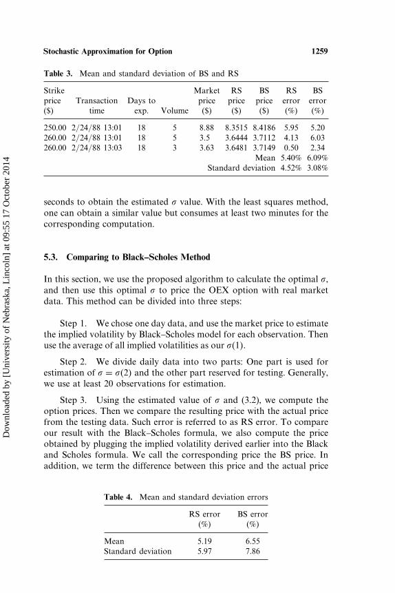
5.3. Comparing to Black–Scholes Method

In this section, we use the proposed algorithm to calculate the optimal ,and then use this optimal to price the OEX option with real marketdata. This method can be divided into three steps:

Step 1. We chose one day data, and use the market price to estimatethe implied volatility by Black–Scholes model for each observation. Thenuse the average of all implied volatilities as our �1�.

Step 2. We divide daily data into two parts: One part is used forestimation of = �2� and the other part reserved for testing. Generally,we use at least 20 observations for estimation.

Step 3. Using the estimated value of and (3.2), we compute theoption prices. Then we compare the resulting price with the actual pricefrom the testing data. Such error is referred to as RS error. To compareour result with the Black–Scholes formula, we also compute the priceobtained by plugging the implied volatility derived earlier into the Blackand Scholes formula. We call the corresponding price the BS price. Inaddition, we term the difference between this price and the actual price

Table 4. Mean and standard deviation errors

RS error BS error(%) (%)

Mean 5.19 6.55Standard deviation 5.97 7.86

Dow

nloa

ded

by [

Uni

vers

ity o

f N

ebra

ska,

Lin

coln

] at

09:

55 1

7 O

ctob

er 2

014

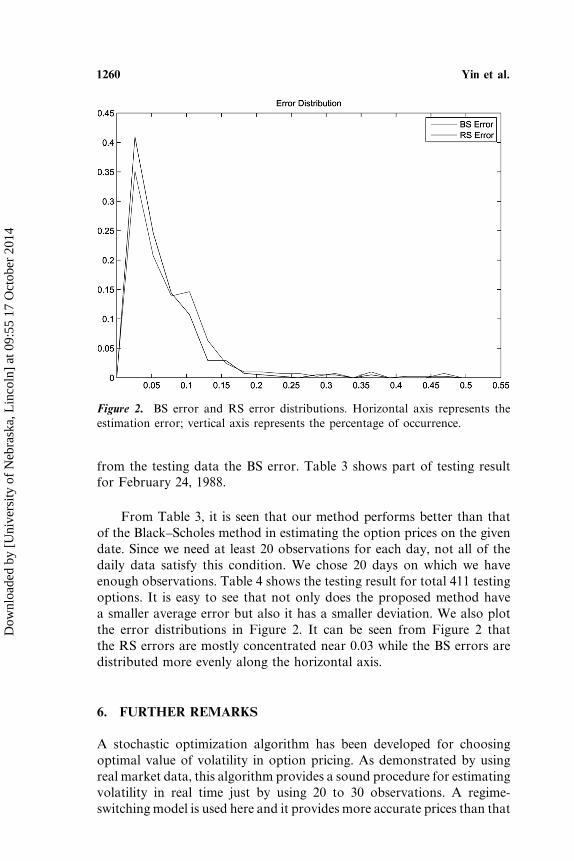
1260 Yin et al.

Figure 2. BS error and RS error distributions. Horizontal axis represents theestimation error; vertical axis represents the percentage of occurrence.

from the testing data the BS error. Table 3 shows part of testing resultfor February 24, 1988.

From Table 3, it is seen that our method performs better than thatof the Black–Scholes method in estimating the option prices on the givendate. Since we need at least 20 observations for each day, not all of thedaily data satisfy this condition. We chose 20 days on which we haveenough observations. Table 4 shows the testing result for total 411 testingoptions. It is easy to see that not only does the proposed method havea smaller average error but also it has a smaller deviation. We also plotthe error distributions in Figure 2. It can be seen from Figure 2 thatthe RS errors are mostly concentrated near 0.03 while the BS errors aredistributed more evenly along the horizontal axis.

6. FURTHER REMARKS

A stochastic optimization algorithm has been developed for choosingoptimal value of volatility in option pricing. As demonstrated by usingreal market data, this algorithm provides a sound procedure for estimatingvolatility in real time just by using 20 to 30 observations. A regime-switching model is used here and it provides more accurate prices than that

Dow

nloa

ded

by [

Uni

vers

ity o

f N

ebra

ska,

Lin

coln

] at

09:

55 1

7 O

ctob

er 2

014

Stochastic Approximation for Option 1261

of the usual Black–Scholes model. The approach developed is simple andsystematic. It can be used for online option pricing and provides usefulguideline for option transactions.

The advantage of the proposed method is its simple recursive form.Compared with the least squares method, it does not require as manyobservations. The simple recursive algorithm often takes only seconds toreach the optimal value. Further effort may be devoted to improve theefficiency and to reduce the variance and bias.

REFERENCES

1. Billingsley, P. 1968. Convergence of Probability Measures. J. Wiley, NewYork.

2. Chance, D.M. 2004. An Introduction to Derivative and Risk Management.South-western College Publisher.

3. Elliott, R.J., and Kopp, P.E. 1998. Mathematics of Financial Markets.Springer-Verlag, New York.

4. Ethier, S.N., and Kurtz, T.G. 1986. Markov Process: Characterization andConvergence. John Wiely, New York.

5. Hull, J.C. 1997. Options, Futures, and Other Derivatives. 3rd Ed.; Prentice-Hall, Upper Saddle River, NJ.

6. Kushner, H.J. 1984. Approximation and Weak Convergence Methods forRandom Processes, with Applications to Stochastic Systems Theory. MITPress, Cambridge, MA.

7. Kushner, H.J., and Yin, G. 2003. Stochastic Approximation and RecursiveAlgorithms and Applications. 2nd Ed.; Springer, New York.

8. Yao, D.D., Zhang, Q., and Zhou, X.Y. 2006. A regime-switching model forEuropean options. In Stochastic Processes, Optimization, and Control TheoryApplications in Financial Engineering, Queueing Networks, and ManufacturingSystems. Yan, H.M., Yin, G., and Zhang, Q. (eds.), Springer, New York,vol. 94, pp. 281–300.

9. Yin, G., Liu, R.H., and Zhang, Q. 2002. Recursive algorithms forstock liquidation: A stochastic optimization approach. SIAM Journal ofOptimization 13:240–263.

10. Zhang, Q. 2001. Stock trading: An optimal selling rule. SIAM Journal ofControl Optimization 40:64–87.

Dow

nloa

ded

by [

Uni

vers

ity o

f N

ebra

ska,

Lin

coln

] at

09:

55 1

7 O

ctob

er 2

014