IEEE TRANSACTIONS ON AUTOMATIC CONTROL, VOL. AC-13, NO. 5, OCTOBER 1968 515

Stochastic Approximation Algorithms for Linear Discrete-Time System Identification

Absiracf-The parameter identification problem in the theory of adaptive control systems is considered from the point af view of stochastic approximation. A generalized algorithm for on-line identi- fication of a stochastic linear discrete-time system using noisy input and output measurements is presented and shown to converge in the mean-square sense. The algorithm requires knowledge of the noise variances involved. It is shown that this requirement is a dis- advantage associated with on-line identification schemes based on minimum mean-squareerror criteria. The paper also presents two off-line identification schemes which utilize measurements obtained from repeated runs of the system's transient response and do not require explicit knowledge of the noise variances. These algorithms converge with probability one to the true parameter values.

I. IKTRODUCTION

T HIS PAPER presents several algorithms for the identification of parameters of linear discrete-time systems operating in a stochastic environment.

Suitable for adaptive control systems, these algorithms are based upon the method of stochastic approximation which has been used for system identification by several authors, e.g., see Ho and Lee [SI, Tsypkin [ l l ] , Sakrison [SI, Kirvaitis and Fu [j], or Saridis, Nikolic, and Fu [9].

First an algorithm is presented which accomplishes on-line identification of stochastic systems with noise contaminated input and output measurements. This algorithm generalizes the original least-square iden- tification schemes presented by Ho and Lee [SI, nhich were shown to converge in the mean-square sense under the restrictions that the transfer function between noise input and system output, have no numerator dynamics and that the output be exactly measurable. The algo- rithm presented here is shown to converge for arbitrary but known numerator dynamics and for noisy measure- ment conditions, provided that the noise variances are specified.

The second part of this paper proposes two stochastic approximation algorithms suited for off-line identifica- tion of linear discrete-time systems. I t is assumed that the transient response of the unknown plant can be cycled repetitively, such that the initial state for each cycle is a sample value from an unknown but stationary probability distribution, or that input-output records are available from which such data can be obtained. Both algorithms converge with probability one, yet no

and May 16, 1968. This work was supported by N.'ASA Institutional Manuscript received April 10, 1967; revised November 7, 1967,

Grant NGR 15-005-021. The authors are n-ith Purdue University, Lafayette, Ind.

knowledge of higher-order noise statistics is required for their implementation. Off-line identification problems of a similar type have been considered previously by Stieglitz and 3IcBride [lo], while analogous results for the case of memoryless systems mere recently obtained in 191.

I I. GEKERALIZED OK-LINE IDESTIFICXTION The problem considered here is the identification of

parameters aT = (al, a2, . . . , a,) and bT = (b l , b2, . . . , b,) in the following lzth order linear discrete-time system:

z(R + 1) = ax@) + bu(k) + dw(R) ; 1

1 aT 1

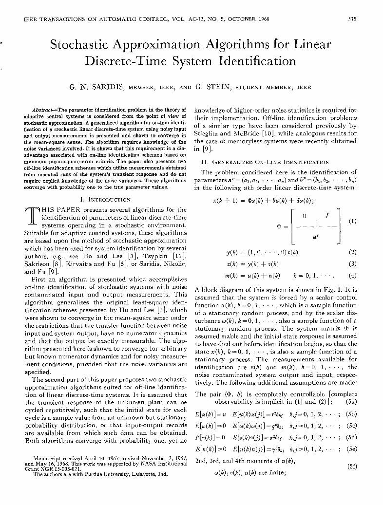
A block diagram of this system is shown in Fig. 1. I t is assumed that the system is forced by a scalar control function u ( k ) , k =0, 1, . . . , which is a sample function of a stationary random process, and by the scalar dis- turbance w ( k ) , k =0, 1, . . . , also a sample function of a stationary random process. The system matrix @ is assumed stable and the initial state response is assumed to have died out before identification begins, SO that the state x ( k ) , K = O , 1, . . . , is also a sample function of a stationary process. The measurements available for identification are e(K) and m ( k ) , k =0, 1, . . . , the noise contaminated system output and input, respec- tively. The following additional assumptions are made:

The pair (a, b ) is completely controllable [complete observability is implicit in (1) and (2) ] ; (5a)

E[u(K)]=u E [ ~ ( R ) . u ( j ) ] = r ~ 6 ~ ~ R , j = O , 1, 2, . . ; (5b)

E [ ~ ( R ) ] = O ~[w(k)w(j)] = q 2 6 k j R , ~ = o , I , 2, . . . ; (jc)

E[c(R)]=O E [ v ( R ) c ( j ) ] = u 2 & , ~ K , j = O , 1, 2, . . * ; (5d)

E [ H ( R ) ] = O ~ [ n ( k ) n C j ) ] = y % ~ ~ K , ~ = o , 1, 2, . . . ; (;e)

2nd, 3rd, and 4th moments of zt(R), (5f)

w ( K ) , ~ ( k ) , t t ( K ) are finite;

516 IEEE TRANSACTIONS ON AUTOMATIC CONTROL, OCTOBER 1968

Fig. 1. The system under consideration.

u ( ~ ) , w ( k ) , ~ ( k ) , n(K) are mutually independent ( j d

(jh)

sequences of independent random variables;

The vector dT = ( d l , d ? , * . , dn) and the noise variances p?, u2, y2 are horn.

As shown in Lee [ 6 ] , (1) and (2) are equivalent to the following difference equation :

y ( k + n ) - a,y(K + IZ - 1) - a,-ly(k + n - 2) - . * *

where

is a composite noise term with the following statistical properties:

E [ Z ( j - 1)50')] # 0 j = 1, 2, - . . (l lc)

3,Iotivated by (lo), the following algorithm is pro- posed for the recursive estimation of vector 4. Let &(k -1) be the estimate of 4 a t the (k -1)th stage of the process. Then

c$(k + .12) = d(K - 1) + p - { Z ( k + 12- 1) [Z(k + t t ) c 3 2

1 q2;

c$(k - 1) - ---

L .I

where the matrix D and the vector d* are defined by

Under the assumptions (5) and the following specifica- tion for the sequence p ( j )

algorithm (12) can be shown to converge in the mean- square sense to the true parameter vector 4. T h a t is, for arbitrary d(0)

where the norm of a vector x is defined as

SARIDIS AND STEIN: STOCHASTIC APPROXIMATION ALGORITHMS 517

The proof of convergence is given in the Appendix. If the last three terms in the braces are removed, algo-

rithm (12) has the same form as the specific identifica- tion algorithms presented by Ho and Lee [3]:

* [ z (k + $2) - ZT(k + 12 - 1)&(k - 111.

Further, if the weighting factor $ ( k -l!n+l) is re- placed by an appropriate matrix P(k+n) given recur- sively by

P ( k + 2 . ) = P(k - 1) - P ( k - l ) Z ( k + f2. - 1)

[ Z T ( k + 72, - 1)P(k - 1 ) z ( k + .7Z - 1) + 11-l

. Z T ( k + n - 1)P(k - 1) (16)

then a version of the least-square estimator [6] is ob- tained. I t has been shown that P ( k ) behaves asympto- tically as l / k [2]. Thus conditions (14) are satisfied in the limit and convergence can still be obtained for this least-square case.

The additional terms in algorithm (12) are introduced by the measurement noises and by the input distur- bance of the system. Their function is simply to correct the statistical bias produced when the above-mentioned specific algorithms are used t o solve the general problem considered here. The term

L I

serves to obtain convergence to the true parameter values under noisy measurement conditions [4], and the two additional terms are required to assure convergence in the presence of the disturbance o(K). I t is important to observe that for the particular circumstances of no measurement noise and vector dT = (0, 0, . . . , 0, d,) (;.e., the transfer function Y ( z ) / W ( z ) has no numerator dynamics), all three correction terms vanish. This is the case for which the specific algorithms were derived in Ho and Lee [SI.

Finally, it is useful to demonstrate that the correction terms of algorithm (12) do not merely act as mathe- matical devices to facilitate a convergence proof, but rather that their absence actually produces a biased estimate. This is pointed out in the Appendix and illus- trated in the following example.

111.. 'EXAMPLE 1

T h e performance of the identification algorithm (12) with weighting matrix (16) is demonstrated on a fourth- order system taken from Lee 161:

0 1 0

0 0 1 x ( k + 1) =

0 0 "I 1 z ( k ) (17) -0.656 0 . f 8 4 -0.18 1

+ d 4 k ) z ( k ) = Xl(k) + c ( k ) .

This application does not require the identification of the control vector b. Consequently, the identification algorithm reduces to the following form:

r$(k + TZ) = r$(k - 1) + P ( k + 1Z) { z (k + 'H - 1) + ( k + 12) - Z T ( k + f 2 - l )d(k - l ) ] (18)

+ cr2r$(k - 1) + q2DDTd(k - 1) - q2d*) .

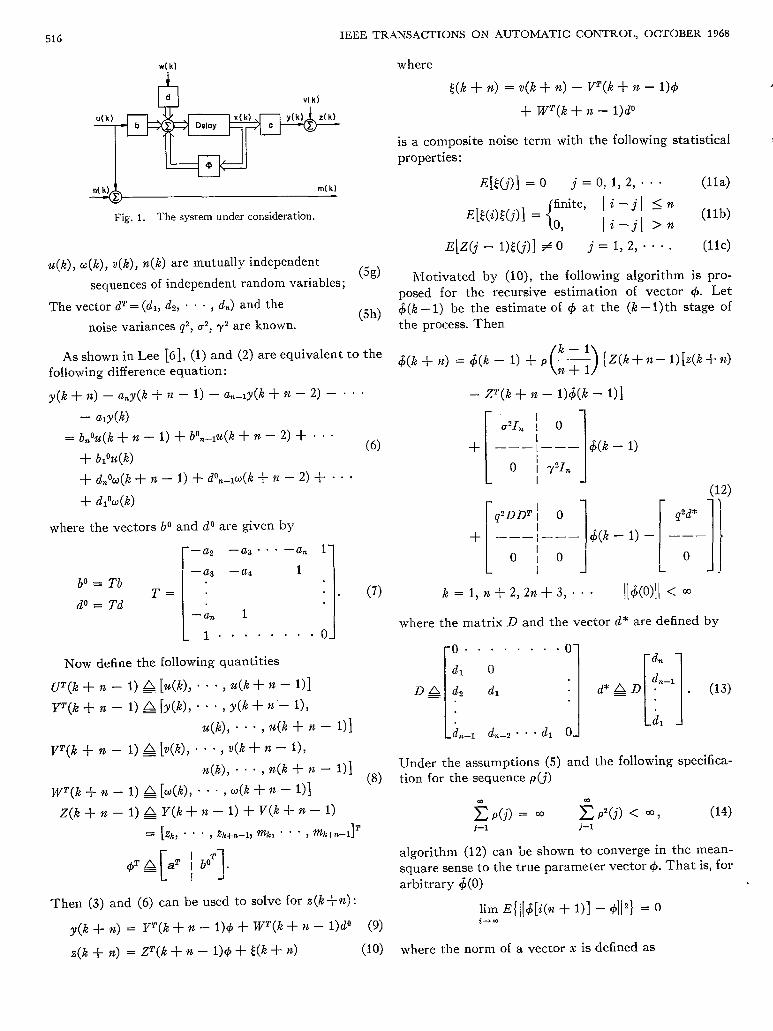
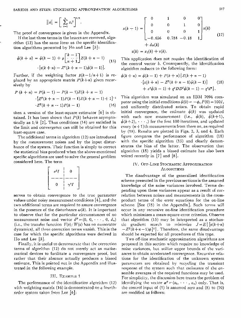
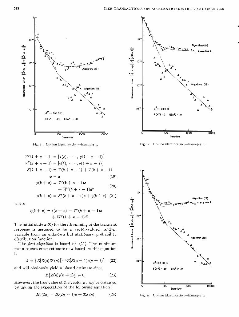
This algorithm was simulated on an IBM 7094 com- puter using the initial conditions $(O) = -4, P(0) = 1001, and uniformly distributed noises. To obtain rapid initial convergence, the estimate d ( k ) was updated with each ne117 measurement (i.e., & ( k ) , & ( k + l ) , &(k+2), . . ,) for the first 100 iterations, and updated every (n +l)th measurements from there on, as required by (18). Results are plotted in Figs. 2, 3, and 4. Each figure compares the performance of algorithm (18) with the specific algorithm (15) and clearly demon- strates the bias of the latter. The observation that algorithm (15) yields a biased estimate has also been voiced recently in [ 7 ] and [8].

IV. OFF-LINE STOCHASTIC APPROXIMATION ALGORITHMS

The disadvantage of the generalized identification scheme presented in the previous sections is the assumed knowledge of the noise variances involved. Terms de- pending upon these variances appear as a result of cor- relation between noises and measurements in the cross- product terms of the error equations for the on-line scheme [See (75) in the Appendix]. Such terms will occur in any recursive on-line identification procedure which minimizes a mean-square-error criterion. Observe that algorithm (15) may be interpreted as a stochas- tic gradient search to minimize J = E { [z (k+n) - Z T ( k +n - 1)412 1 . Therefore, the same disadvantage should be expected for all procedures of this type.

Two off-line stochastic approximation algorithms are proposed in this section which require no knowledge of noise variances, but utilize upper bounds of the vari- ances to obtain accelerated convergence. Recursive rela- tions for the identification of the unknown system parameters are obtained by recycling the transient response of the system such that estimates of the en- semble averages of the required functions may be used. For simplicity, the discussion here treats the problem of identifying the vector aT= (a l , . . . , a,) only. Tha t is, the control input of (1) is assumed zero and (8) to (10) are modified as follows:

51 8 IEEE TRXISACTIONS O N AUTOMATIC CONTROL, OCTOBER 1968

E(vt) = .25 E(w*) = 1.0 A

I 100 1000 10000

Iterations

Fig. 2. On-line identification-Example 1.

Y T ( k + I2 - 1 = [ y ( k ) , . . . , y ( k + 12 - l)]

V T ( k + 12 - 1) = ['d(k), . . . , f I ( K + n - l)]

Z ( k + I2 - 1) = Y ( k + ?Z - 1) + V ( k + n - 1)

+ = a (19) y ( k + E.) = YT(k + fz - 1)a

(20) + W ( k + I t - 1)dO

s(k + n) = ZT(k + ?Z. - 1). + E(k + 12) (21)

where

[ ( k + %) = C(k + 11.) - V T ( k + 72 - 1)a

+ T V ( k + n - l)#.

The initial state x i ( 0 ) for the ith running of the transient response is assumed to be a vector-valued random variable from an unknown but stationary probability distribution function.

The jirst algorithm is based on (21). The minimum mean-square-error estimate of a based on this equation is

ci = { E[Z(n)ZT(~Z)~)- 'E[Z(~z - l)Z(it + l)] (22)

E { Z(n)E(n + 111 f 0. (23)

and will obviously yield a biased estimate since

However, the true value of the vector a may be obtained by taking the expectation of the following equation:

Mi(2n) = B42n - 1)a + Z:i(2n> (24)

1.

A

A .

A

\ Algorithm (18)

d T = ( O I O I ) A A\* E(v*) = 0 E(wt) = 1.0

IO 100 1000 loo00 Iterations

Fig. 3 . On-line identification-Example 1.

E(ve) =.25 E(wP)=I.0

IO 100 1000 10000 Iterations

Fig. 4. On-line identification-Example I.

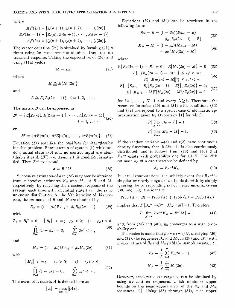
SARIDIS AND STEIN: STOCHASTIC APPROXIMATION ALGORITHMS 519

where

~ ~ ~ ( 2 n ) = [.zi(n + 11, z i ( n + 21, . . , zi(2n)]

BiT(2n - 1) = [Zi(n), Zi (n + l ) , . . . , Zi(212 - I ) ]

~ ( 2 n ) = [ti(% + 11, tdn + 21, - . , t d 2 1 2 ) I .

The vector equation (24) is obtained by forming (21) n times using 2n measurements obtained from the ,ith transient response. Taking the expectation of (24) and using ( l l a ) yields

M = Ba (25 )

where

and

The matrix B can be expressed as

or

BT = { (PE[x(O)], (P2E[.2:(0)], . . . , (P,"E[x(O)] } . (27 )

Equation (27) specifies the condit ion for identi$cation for this problem. Parameters a of system ( 1 ) with ran- dom initial state x ( 0 ) and no control input are iden- tifiable if rank ( B T ) =n. Assume this condition is satis- fied. Then B-l exists and

a = B-'M. (28)

Successive estimates of a in (28) may now be obtained from successive estimates BX and l l f A r of B and X , respectively, by recycling the transient response of the system, each time with an initial state from the same unknown distribution. At the Nth iteration of this pro- cess, the estimates of B and X are obtained by

BN = ( 1 - Px)Bx--1 + /3xBAv(21~ - 1 ) ( 2 9 )

wit 11

Bo = BoT > 0 ; I Bo1 < 00 ; ,8x > 0 ; ( 1 - 837) > 0 ;

The norm of a matrix A is defined here as

I A I = max IIAXII. I I 4 I=1

for i = 1 , . . . , N - 1 and every 1 V 2 l . Therefore, the recursive formulas (29) and (31) with conditions (30) and (32) correspond to a special case of stochastic ap- proximation given by Dvoretzky [ l ] for which

P [ lim BN = B ] = 1 (38)

P [ lim Mnr = M ] = I . (39)

AT-. m

N-. m

If the random variable w ( k ) and v ( k ) have continuous density functions, then Bi(2n - 1 ) is also continuously distributed, and it folloxys from (29) and (30) that Bs-l exists with probability one for all N . The Nth estimate & of a can therefore be defined by

SA- = BN-~MAT. (40)

In actual computations, the unlikely event that Bx-l is singular or nearly singular can be dealt with by simply ignoring the corresponding set of measurements. Given (38) and (39) , the identity

Prob ( A + B) = Prob ( A ) + Prob ( B ) - Prob ( A B )

implies that P [Bx-I4B-l, Ms+M] = 1. Therefore

P[ lim BN-~LM,V = B-lM] = 1 (41) x+ m

and, from ( 2 8 ) and (40), converges to a with prob- ability one.

If a choice is made that ON =PA- = l/N, satisfying (30) and (32), the sequences B N and M A - in (29) and (31) with proper values of Bo and ?!To yield the sample means, i.e.,

(42)

1 .%*

-1: i-1 M N = 7 Mi(2tZ). (43)

However, accelerated convergence can be obtained by using PT and p~ sequences which minimize upper bounds on the mean-square error of the B.v and M A -

sequences [9] . Using (33) through (37), such upper

520 IEEE TRANSACTIONS ON AUTOMATIC CONTROL, OCTOBER 1968

E { ~ ~ M N - M i l ? ) 5 pNT,2 s 2 I.

The inequalities (46) and (47) imply that the sequences E { I (BAT -B)'I 1 and E { 1 1 & - -141 2 } are monotonically decreasing. Therefore, assuming

bo 2 E { 1 (Bo - B)'I } (48)

mo 2 B{IIMo - M p } (49)

and iterating (46) and (47), the following is obtained:

These sequences BS and p~ satisfy (30) and (32) and thus qualify for the recursive algorithms (29) and (31), respectively. Such schemes are demonstrated in the example which follows.

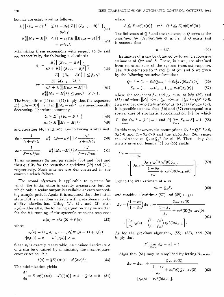
The second algorithm is applicable to systems for which the initial state is exactly measurable but for which only a scalar output is available at each succeed- ing sample period. Again it is assumed that the initial state x ( 0 ) is a random variable with a stationary prob- ability distribution. Using (l), (2), and (3) with ~ ( k ) = O for all k, the following equation may be written for the ith running of the system's transient response:

z f (n ) = aTxi(0) + O , ( I Z ) (52)

where

e,(.) = (dn, L ~ , . . . , dl)wi(?l - 1) + vi(.) E[&(n)] = 0 E[ei'(n)] < Q;.

Since x. is exactly measurable, an unbiased estimate S of a can be obtained by minimizing the mean-square- error criterion [9] :

J ( a ) = + ~ f ( z ( n ) - x~(0)a)2}. (53)

The minimization yields

dJ da - = E {x(O)(z(,z) - xT(0)a) 1 = s - Q 1, = 0 (54)

u-here

S E{x(O)z(n) j and Q-'& E(x (0 )xT(O) ) .

The finiteness of Q - l and the existence of Q serve as the conditions for identification of a ; i.e., if Q exists and is nonzero then

a = QS. ( 5 5 )

Estimates of a can be obtained by forming successive estimates of Q - l and S. These, in turn, are obtained from repeated runs of the system transient response. The Nth estimates Q-v-l and of p1 and S are given by the following recursive formulas:

QN-' = (1 - PN)QX-I-' + BN[xN(0)xNT(O) ] (56)

SN = (1 - PX)SN-l + P N [ x N ( O ) z N ( r z . ) ] (57)

where the sequences /3.~ and p . ~ must satisfy (30) and (32) and where (ISol( <=, I Q O I < x , and Q0-l = Q P 1 > O . In a manner completely analogous to (33) through (39), i t is possible to show that (56) and (57) correspond to a special case of stochastic approximation [l] for which

P[ lim Qx-l = Q-l] = 1 and P [ lim SAT = S ] = 1. (58)

In this case, however, the assumptions Qo-'= Q O T - l > 0, @.v>O and (1 -PAT) > O and the algorithm (56) assure the existence of Q N = QATT for all N. Then using the matrix inversion lemma [6] on (56) yields

x- = N + =

1 QN = ~

1 - O N

Q N - - I ~ N ( O ) ~ N ~ ( O ) Q N - - I I- (59) h'-1 -

1 - @N

PN x.?.'(o)gN-lxX(o>

Define the Nth estimate of a as

S N = QNSN (60)

and combine algorithms (57) and (59) to get

1 - P N Q N - I . T N ( ~ )

1 - PN ,, + ~ ~ ( O ) Q A ~ - ~ X N ( O ) PN

As for the previous algorithm, (55), (58), and (60) imply that

P[ Iim SX = a ] = I. x+ a

Algorithm (61) may be simplified by letting PN=PAT: Q N - I ~ N ( ~ )

+ ~ N ' ( O ) Q N - - ~ X N ( O ) (62)

S N = dN-1 + 1 - P N

PN

' [zN(?z) - xN'(O)si.N--l].

SARIDIS AND STEIN: STOCHASTIC APPROXIMATION ALGORITHMS

where

PX = L V + rq?/qo

E { I ( Q x - l - Q - 9 ' 1 f 5 Lj7 + r q 2 / q o TQ2

x + r,2jso

7 8 %

:I7 + T-s'/so

(66)

1 PM =

(67) E{IIsA- - S/i2f I

Tq2 2. E { I ( % v ( 0 ) X N T ( O ) - Q9q f r,2 2. Ef / (Xh- (O) .%v(H~) - SI/')

and

q o 2 E { I (Qo-' - Q-')'I 1 So 2 E(IISo - Si12}.

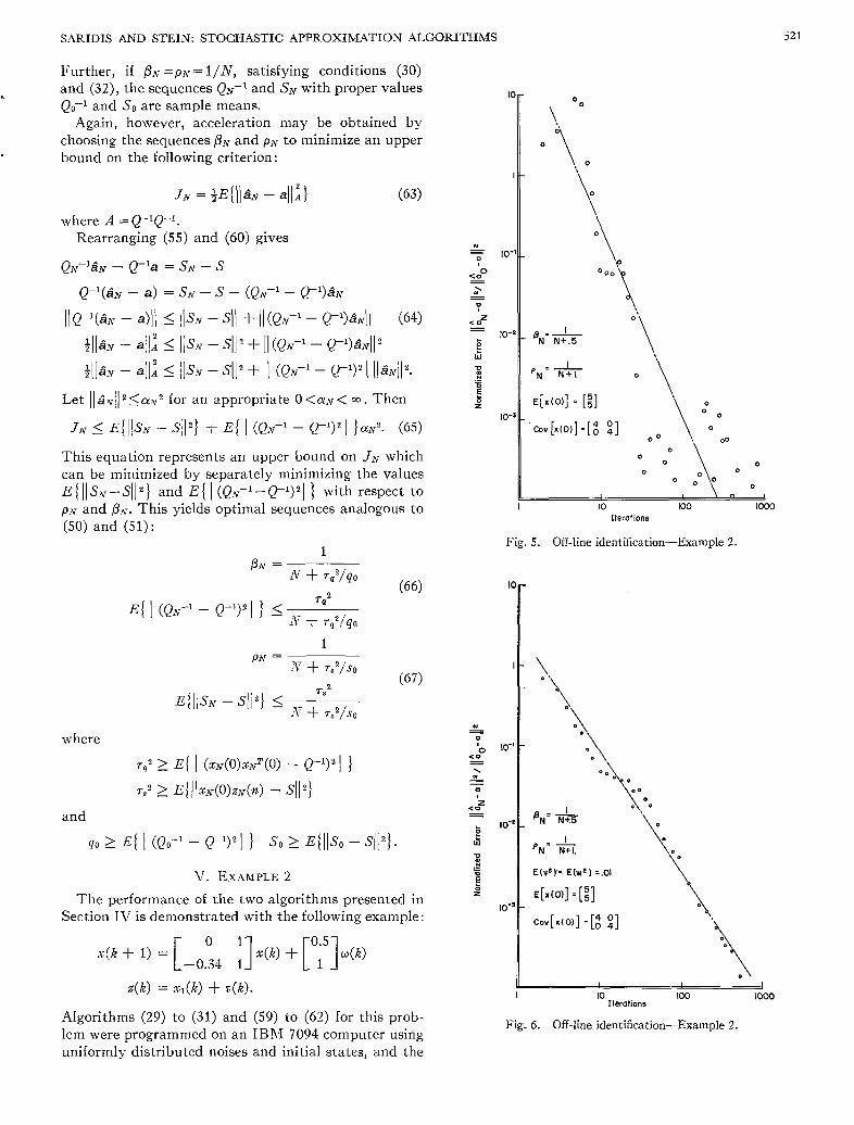
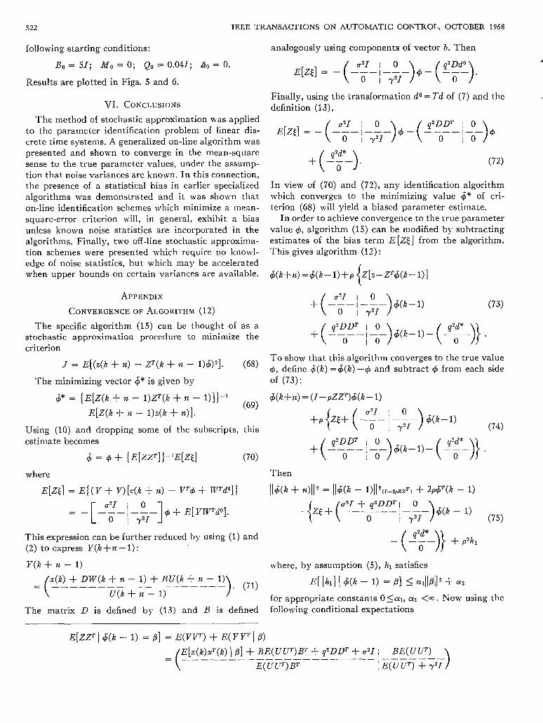
V. EXAMPLE 2

T h e performance of the two algorithnls presented in Section IV is demonstrated with the following example:

s(K 4- 1) = [ '1 r(K) + [ O ; ] u ( R ) 0

-0.34 1

z (k) = x,@) + o ( K ) . I 10 1 0 0 1000

Algorithms (29) to (31) and (59) to (62) for this prob- lem were programmed on an IBhl 7094 computer using uniformly distributed noises and initial states, and the

Iterations

Fig. 6 . Off-line identification-Example 2.

522 IEEE TRANSACTIONS ON AUTOMATIC CONTROL, OCTOBER 1968

following starting conditions:

Bo = 51; M o = 0; Qo = 0.041; do = 0.

Results are plotted in Figs. 5 and 6.

VI. COKCLUSIONS

The method of stochastic approximation was applied to the parameter identification problem of linear dis- crete time systems. A generalized on-line algorithm was presented and shown to converge in the mean-square sense to the true parameter values, under the assump- tion that noise variances are known. In this connection, the presence of a statistical bias in earlier specialized algorithms was demonstrated and i t was shown that on-line identification schemes which minimize a mean- square-error criterion d l , in general, exhibit a bias unless known noise statistics are incorporated in the algorithms. Finally, two off -line stochastic approxima- tion schemes were presented which require no knowl- edge of noise statistics, but which may be accelerated when upper bounds on certain variances are available.

APPENDIX

CONVERGENCE OF ALGORITHM (1 2)

The specific algorithm (15) can be thought of as a stochastic approximation procedure to minimize the criterion

J = E [ ( z ( k + H) - Z T ( k + W, - 1)&'] . (68)

The minimizing vector 6* is given by

rj* = { E [ Z ( k + 12 - 1 ) Z T ( K + 12 - 1)]}-1 (69)

E [ Z ( k + - l)a(k + ?&)I. Using (10) and dropping some of the subscripts, this estimate becomes

r j = C + { EIZZT])-lEIZEI (70)

where

E[Zt] = E ( ( I ' 4- V ) [ ~ ( k + 12) - VTQ + wTdO]}

This expression can be further reduced by using (1) and (2) to express Y(k +n - 1) :

Y(k + n - 1 )

~ ( k ) + DW(k + fi - 1) + B U ( k + ?Z - 1) U(k + n - 1)

The matrix D is defined by (13) and B is defined

analogously using components of vector b. Then

Finally, using the transformation do = Td of (7) and the definition (13),

+ (q-). In view of (70) and (72), any identification algorithm which converges to the minimizing value &* of cri- terion (68) will yield a biased parameter estimate.

In order to achieve convergence to the true parameter value 4, algorithm (15) can be modified by subtracting estimates of the bias term E [ Z t ] from the algorithm. This gives algorithm (12):

r j (k+n) = r j ( k - l ) + p Z [ B - F r j ( k - l ) ]

T o show that this algorithm converges to the true value 4, define B;(k) =$(k) -4 and subtract 4 from each side of (73):

$@+E) = ( I - p Z Z T ) B ; ( k - l )

where, by assumption (5), hl satisfies

E [ l J 2 l l I B;(k - 1) = PI 5 (111(811? + (12

for appropriate constants O<al, cy2 <a!. Now using the following conditional expectations

SARIDIS AND STEIN: STOCHASTIC APPROXIMATION PLGORITHMS 523

and [by assumption (5g)l

- W t I 4@ - 1) = PI = m 6 1 ,

the conditional expectation of (75) becomes

By assumption (Sb), the n X n matrix E(UUT) is posi- tive definite. Further, under the controllability condi- tion on the pair (a, b ) , the n X n matrix E [ x ( k ) ~ T ( k ) I &(k-1) = p ] is also positive definite. In the absence of a control input, this matrix will still be positive definite if (a, d ) is a controllable pair. In this case, the vector bo is deleted from r$ and simplified versions of the above steps are valid. See example in Section 111. With both E(UUT)>O and E[x(k)xT(k)I,3]>0, the entire 2 n X 2 7 2 matrix in the second term of (76) is positive definite. Let its minimum eigenvalue by Xa>O. Then

E[II4(K + 4 1 1 2 1 5 (1 - m o + P’.I).E[Ilm - 1)pl (77) + P?cr22.

Under conditions (14), this equation satisfies the re- quirements of a convergence proof due to Dvoretzky [l, sec. 81 from which the desired conclusion follows:

lim ~ [ l l 4 [ i ( n + l)]!i’] = 0. i+ (E

REFEREXCES [l] A . Dvoretzky, “On stochastic approximation,” Proc. 3rd Berke-

[2] Y . C. Ho, “On the stochastic approximation method and optimal ley Synp. on Matk. Stat. a.nd Probability, vol. 1, 1956.

filtering theory,‘’ J . Math. Anal. and Appl., vol. 6, pp. 152-154, 1963.

[3] Y . C. Ho and R. C. K. Lee, “Identification of linear dynamic systems,” Proc. 3rd Spnp. on Adaptive Pmcesses, 1964.

[ 4 Y . C. Ho and B. H. Whalen, “An approach to the identification and control of linear dynamic systems with unknown param- eters,” IEEE Trans. Automatic Control (Correspondence), vol. AC-8, pp. 255-256, July 1962.

[5] K. Kirvaitis and K. S. Fu, Identification of nonlinear systems by stochastic approximation,” J a C C Preprints, 1966.

[6] R. C. K. Lee, Optiwzal Estimation, Identz$cation and Cont~ol, Research Rlonograph 28. Cambridge, Mass.: 5I.I.T. Press, 1964.

[SI R. Roy and K. W. Je:kins, “Identification and control of a flexible launch vehicle, N’ASA Contractor Rept. NAS.3 CR-

[8] D. L. Sakrison, “An approach to the system identification prob- 551, August 1966.

lem,“ Electronics Research Lab., University of California, Berkeley, RIemo ERL-RIlil, July 1966.

[9] G. Saridis, Z. J. Kikolic, and K. S. Fu , “Stochastic approxima-

composition of mixtures,’’ Pmc. 5th. AlZerton Conf. on Circzd tion algorithms for system identification, estimation and de-

a.nd System Tlteorg, 1967. [lo] K. Stieglitz and L. E. McBride, “ A Technique for the identifica-

Papers), vol. AC-10, pp. 461-464, October 1965. tion of linear systems,” IEEE Trans. .424towzati‘ Control (Short

[ l l ] Ya. Z. Tsypkin, “-Adaptation, training and self-organization in automatic systems,”ilotolnatikai Telemekhanika. vol. 27, pp. 23- 61, January 1966.

George N. Saridis ($1’62) was born in Athens, Greece, on November 17, 1931. He received the diploma in mechanical and electrical engineering from the Na- tional Technical University of Athens in 1955, and the M.S.E.E. and Ph.D. degrees from Purdue University, Lafay- ette, Ind., in 1962 and 1965, respec- tively.

From 1955 to 1961, he was an In- structor in the Department of Mechani- cal and Electrical Engineering of the National Technical University of

Athens. From 1963 to 1965, he was an Instructor a t the School of Electrical Engineering, Purdue University, where he has been an Assistant Professor since 1965.

Dr. Saridis is a member of Sigma Xi, Tau Beta Pi, and Eta Kappa Nu.

Gunter Stein (S’67) was born in Bordes- holm, Germany, on July 16, 1941. He received the B.E.E. degree from General Motors Institute, Flint, Mich., in 1966, and the M S . degree from Purdue Uni- versity, Lafayette, Ind., also in 1966. He is currently working toward the Ph.D. degree in the general area of adaptive control systems a t Purdue University, where he is a Graduate Instructor.