Stochastic algorithms in nonlinear regression

Computational Statistics & Data Analysis 33 (2000) 277–290www.elsevier.com/locate/csda

Stochastic algorithms innonlinear regression

Ivan K�riv�ya ;∗, Josef Tvrd��kb, Radek Krpeca

aDepartment of Mathematics, University of Ostrava, Ostrava, Czech RepublicbDepartment of Computer Science, University of Ostrava, Ostrava, Czech Republic

Received 1 March 1998; received in revised form 1 May 1999

Abstract

Recently, the authors have described two stochastic algorithms, based on the controlled randomsearch, for the global optimization. This paper deals with the use of these algorithms in estimatingthe parameters of nonlinear regression models. Several criteria like residual sum of squares, sum ofabsolute deviations and sum of trimmed squares are chosen. The algorithms are experimentally testedon a set of the well-known tasks chosen in such way that most classical techniques based on objectivefunction derivatives fail while treating them. The basic features of the algorithms (rate of convergenceand reliability) as well as their applicability to nonlinear regression models are discussed in more detail.c© 2000 Elsevier Science B.V. All rights reserved.

Keywords: Stochastic algorithms; Controlled random search; Evolutionary search; Global optimization;Regression models

1. Introduction

We consider the following optimization problem: For a given objective functionf : → R; ⊂Rd, the point x∗ is to be found such that

f(x∗) = minx∈

f(x):

The space is de�ned as

=d∏

i=1

〈ai; bi〉; ai ¡bi; i = 1; 2; : : : ; d:

∗ Corresponding author.

0167-9473/00/$ - see front matter c© 2000 Elsevier Science B.V. All rights reserved.PII: S 0167-9473(99)00059-6

278 I. K�riv�y et al. / Computational Statistics & Data Analysis 33 (2000) 277–290

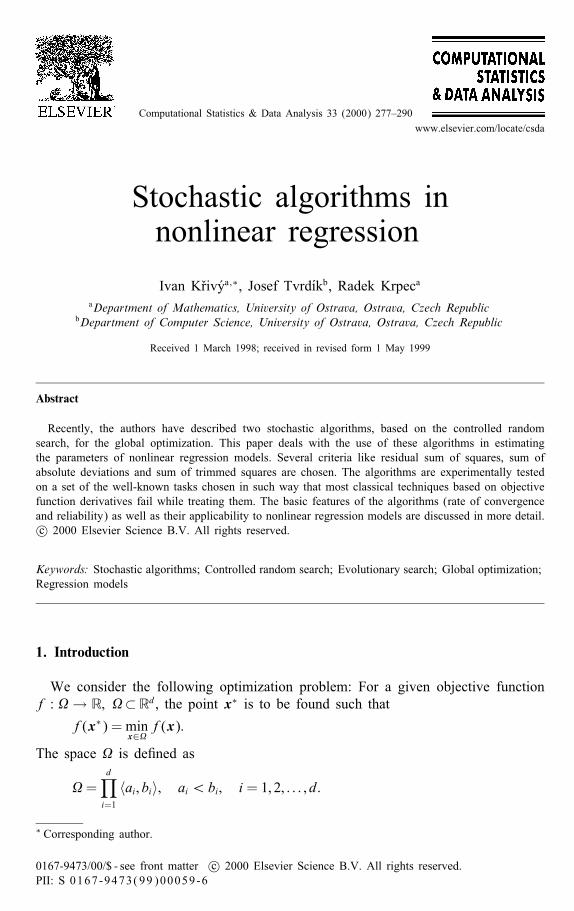
Fig. 1. Scheme of the re ection for d= 2.

We proposed some stochastic algorithms (K�riv�y and Tvrd��k, 1995, 1996; Tvrd��kand K�riv�y, 1995) based on the controlled random search (CRS) of Price (1976)and we applied them to estimate the parameters of nonlinear regression models. Inthis contribution we consider only two of the algorithms, namely the algorithm ofmodi�ed controlled random search (MCRS) and the evolutionary search (ES2).The algorithms are based on the procedure Re ection that serves for generating

the next trial point. Given a population, P, consisting of N randomly taken pointsin , the new trial point x is generated from a simplex (a set of d + 1 linearlyindependent points of a population P in ) by the relation

x= g − Y (z − g); (1)

where z is one (randomly taken) pole of the simplex S, g the centroid of the re-maining d poles of the simplex and Y a random multiplication factor. This point xmay be considered as resulting from the re ection of the point z with respect to thecentroid g (see Fig. 1).

2. MCRS algorithm

Starting from the procedure Re ection, our MCRS algorithm can be formallydescribed as follows:

procedure MCRS;begin P:= population of N uniformly distributed points in ,

repeatrepeat x:=Re ection(P; x) until x ∈ ;if f(x)¡f(xmax) then xmax:=x;

until stopping condition is true;end {MCRS};xmax being the point with the largest function value of the N points stored. In con-trast to some recent modi�cations of CRS algorithms (Ali et al., 1997), no localoptimization techniques are used.

I. K�riv�y et al. / Computational Statistics & Data Analysis 33 (2000) 277–290 279

The principal modi�cation of the original Price’s re ection (1976) consists inrandomizing the search for the next trial point. Regarding the multiplication factor Y ,three cases were tested in more detail:

• Y = � (constant),• Y is a random variable with uniform distribution on the interval (0; �),• Y is a random variable with normal distribution N(�; 1).

The best results were obtained when considering Y distributed uniformly with �ranging from 4 to 8 (K�riv�y and Tvrd��k, 1995).When treating regression models, the following functions f are considered as

optimization criteria:

• residual sum of squares (RSS),

RSS =n∑

i=1

r2i ;

• trimmed squares including 80% of the least-squared residuals (TS),

TS =h∑

i=1

(r2)i:n;

• sum of absolute deviations (SAD),

SAD =n∑

i=1

|ri|;

where ri (i = 1; 2; : : : ; n) denote the residuals, n the total number of observations(sample size), h the largest integer less or equal to 4n=5 + 1 and (r2)1:n ≤ (r2)2:n ≤· · · ≤ (r2)n:n the ordered squared residuals.The MCRS algorithm given above includes no particular stop condition. However,

it is clear that the condition has to be evaluated within each iteration of the algorithm.We propose (K�riv�y and Tvrd��k, 1995) to stop the optimization process, when

f(xmax)− f(xmin)f0

≤ �; (2)

where xmin and xmax denote the points with the least and the largest function values,respectively, � a positive input value and f0 an appropriate constant factor re ectingthe variability of the dependent model variable. For example, when using RSS or TSas the optimization criterion, the f0 factor can be equal to the total sum of squareddi�erences of the observed values from their average. Similarly, in case of SADcriterion f0 can give the total sum of absolute deviations from the average. The stopcondition (2) proves to be more useful than that de�ned by Conlon (1992) becauseof its independence on the objective function values.The inputs to MCRS algorithm consist of:

• number of points, N , to hold in the store,• value of �,• value of � in (2).


3. Evolutionary search

Evolutionary search simulates the mechanisms of natural selection and naturalgenetics, which in general tend to reach optimum (Michalewicz, 1992; Kvasni�ckaand Posp��chal, 1997). Our ES2 algorithm is based on the following principles:

• The initial population is generated randomly in .• The new population inherits the properties of the old one in two ways:

◦ directly by surviving the best individuals (with respect to f-values),◦ indirectly by applying the Re ection procedure to the old population.

• An individual with new properties (even with a larger f-value) is allowed toarise with a small probability p0, something like mutation probability in geneticalgorithms (Goldberg, 1989).ES2 algorithm can be described formally as follows (K�riv�y and Tvrd��k, 1996):

procedure ES2;begin P:= population of points x[1]; : : : ; x[N ] uniformly distributed in ;repeat

m:= random integer from 〈1; M 〉 {M is an input parameter}for j:=1 to m do y[j]:=x[j];i:=m;while i¡N dobegin repeat

repeat x:=Re ection(P; x) until x ∈ ;until f(x) ≤ f(xmax)i:=i + 1;y[i]:=x

end {while}if random¡p0 thenbegin j:= random integer from interval 〈1; N 〉;

replace y[j] with randomly taken point in end {if}P:= population of points y[1]; : : : ; y[N ];

until stopping condition is trueend {ES2}In this algorithm the simplex points are taken completely at random from a currentpopulation. There is, however, another possibility of constructing simplexes: each ofthe simplex points is taken with the probability proportional to its �tness given by(K�riv�y and Tvrd��k, 1997)

si =1

1− N [(1− �)i + �− N ];where i denotes the rank of xi when all points are ordered in a nondecreasingsequence with respect to their f-values and � is a small positive real number.Each of the optimization criteria listed in Section 2 can be applied. Regarding the

stopping condition, we recommend to use relation (2).


When compared with MCRS algorithm, there are two additional input parameters:

• mutation probability, p0,• number, M , of the best points surviving from the old population to the new one.

It is worth noting that ES2 algorithm almost coincides with the MCRS one whenp0 = 0 and M = 0.

4. Test problems

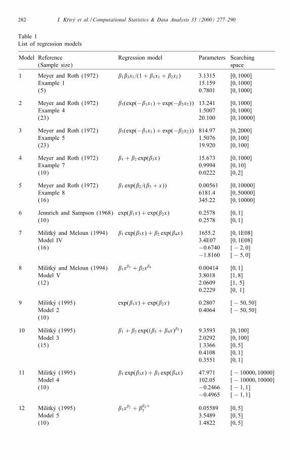
Both algorithms were tested when estimating the parameters of 14 nonlinear re-gression models whose list is given in Table 1.The original data whose references are given in the second column of Table 1 are

summarized in our paper (Tvrd��k and K�riv�y, 1995). The last two columns of thistable show the optimum values of parameters and the size of searching space .The estimate of parameters of these nonlinear regression models is a di�cult task

for classical algorithms of optimization built in a standard statistical software. Wetried to use several standard packages for least-squares estimation of parameters,namely NCSS 6.0, where Levenberg–Marquardt algorithm is used, S-PLUS 4.5 us-ing Gauss–Newton (GN) algorithm, SPSS 8.0 with modi�ed Levenberg–Marquardtalgorithm and SYSTAT 7.0 where both modi�ed GN algorithm and simplex methodare implemented. The starting values of parameters were chosen at random fromacceptable intervals, for each model 100 independent attempts were performed. As itcan be seen from Table 2, algorithms failed frequently in �nding the global minimumof residual sum of squares.

5. Experimental results

Both algorithms were implemented in TurboPascal, version 6.0, and the corre-sponding programs were tested on PC. All listed optimization criteria (objectivefunctions) were applied to each of the regression models, at least 100 independentruns for each model being carried out.The speci�cation of the search domain was always identical for both algorithms.

When estimating the regression model parameters, the common inputs were set asfollows:

• N = 5d,• �= 8,• �= 1E− 15 for RSS and TS criteria and 1E− 8 for SAD criterion.Additional tuning parameters for ES2 algorithm were adjusted to their default

values, namely:

• pm = 0:01,• M = bN=2c, i.e. the largest integer less than or equal to N=2.


Table 1List of regression models

Model Reference Regression model Parameters Searching(Sample size) space

1 Meyer and Roth (1972) �1�3x1=(1 + �1x1 + �2x2) 3.1315 [0; 1000]Example 1 15.159 [0; 1000](5) 0.7801 [0; 1000]

2 Meyer and Roth (1972) �3(exp(−�1x1) + exp(−�2x2)) 13.241 [0; 1000]Example 4 1.5007 [0; 1000](23) 20.100 [0; 10000]

3 Meyer and Roth (1972) �3(exp(−�1x1) + exp(−�2x2)) 814.97 [0; 2000]Example 5 1.5076 [0; 100](23) 19.920 [0; 100]

4 Meyer and Roth (1972) �1 + �2 exp(�3x) 15.673 [0; 1000]Example 7 0.9994 [0; 10](10) 0.0222 [0; 2]

5 Meyer and Roth (1972) �1 exp(�2=(�3 + x)) 0.00561 [0; 10000]Example 8 6181.4 [0; 50000](16) 345.22 [0; 10000]

6 Jennrich and Sampson (1968) exp(�1x) + exp(�2x) 0.2578 [0; 1](10) 0.2578 [0; 1]

7 Militk�y and Meloun (1994) �1 exp(�3x) + �2 exp(�4x) 1655.2 [0; 1E08]Model IV 3:4E07 [0; 1E08](16) −0:6740 [− 2; 0]

−1:8160 [− 5; 0]8 Militk�y and Meloun (1994) �1x�3 + �2x�4 0.00414 [0; 1]

Model V 3.8018 [1; 8](12) 2.0609 [1, 5]

0.2229 [0, 1]

9 Militk�y (1995) exp(�1x) + exp(�2x) 0.2807 [− 50; 50]Model 2 0.4064 [− 50; 50](10)

10 Militk�y (1995) �1 + �2 exp((�3 + �4x)�5 ) 9.3593 [0; 100]Model 3 2.0292 [0; 100](15) 1.3366 [0; 5]

0.4108 [0; 1]0.3551 [0; 1]

11 Militk�y (1995) �1 exp(�3x) + �2 exp(�4x) 47.971 [− 10000; 10000]Model 4 102.05 [− 10000; 10000](10) −0:2466 [− 1; 1]

−0:4965 [− 1; 1]

12 Militk�y (1995) �1x�2 + ��2=x3 0.05589 [0; 5]

Model 5 3.5489 [0; 5](10) 1.4822 [0; 5]


Table 1 (Continued.)

Model Reference Regression model Parameters Searching(Sample size) space

13 Militk�y (1995) �1 + �2x�31 + �4x

�52 + �6x

�73 1.9295 [− 5; 5]

Model 6 2.5784 [− 5; 5](24) 0.8017 [0; 10]

−1:2987 [− 5; 5]0.8990 [0; 10]0.01915 [− 5; 5]3.0184 [0; 10]

14 Militk�y (1995) �1 ln(�2 + �3x) 2.0484 [0; 100]Model 7 18.601 [0; 100](12) 1.8021 [0; 100]

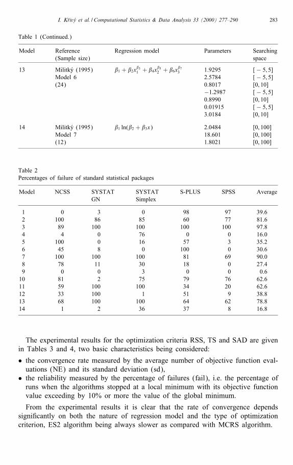
Table 2Percentages of failure of standard statistical packages

Model NCSS SYSTAT SYSTAT S-PLUS SPSS AverageGN Simplex

1 0 3 0 98 97 39.62 100 86 85 60 77 81.63 89 100 100 100 100 97.84 4 0 76 0 0 16.05 100 0 16 57 3 35.26 45 8 0 100 0 30.67 100 100 100 81 69 90.08 78 11 30 18 0 27.49 0 0 3 0 0 0.610 81 2 75 79 76 62.611 59 100 100 34 20 62.612 33 100 1 51 9 38.813 68 100 100 64 62 78.814 1 2 36 37 8 16.8

The experimental results for the optimization criteria RSS, TS and SAD are givenin Tables 3 and 4, two basic characteristics being considered:

• the convergence rate measured by the average number of objective function eval-uations (NE) and its standard deviation (sd),

• the reliability measured by the percentage of failures (fail), i.e. the percentage ofruns when the algorithms stopped at a local minimum with its objective functionvalue exceeding by 10% or more the value of the global minimum.

From the experimental results it is clear that the rate of convergence dependssigni�cantly on both the nature of regression model and the type of optimizationcriterion, ES2 algorithm being always slower as compared with MCRS algorithm.


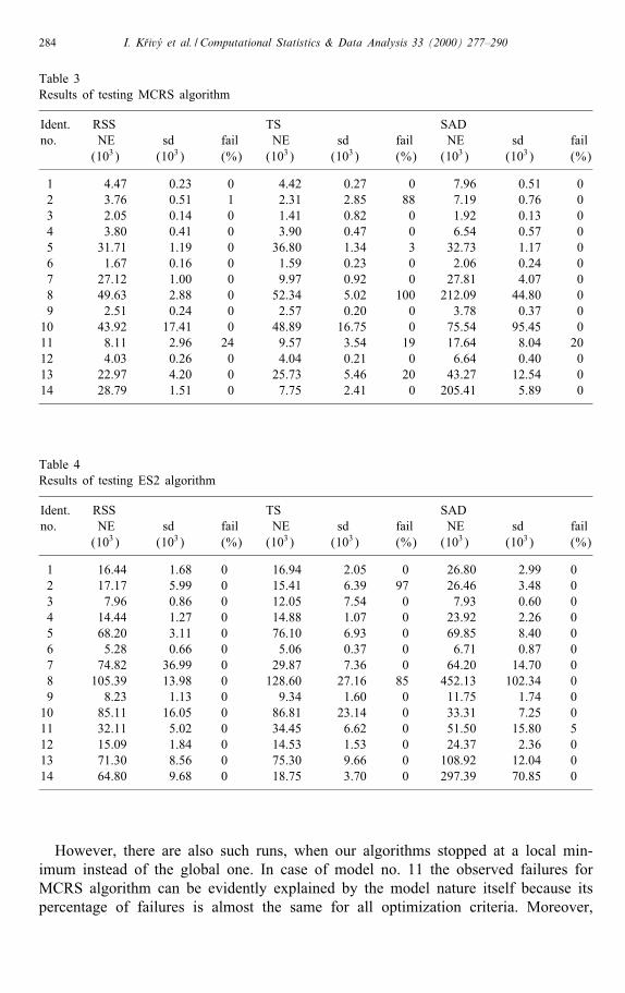
Table 3Results of testing MCRS algorithm

Ident. RSS TS SADno. NE sd fail NE sd fail NE sd fail

(103) (103) (%) (103) (103) (%) (103) (103) (%)

1 4.47 0.23 0 4.42 0.27 0 7.96 0.51 02 3.76 0.51 1 2.31 2.85 88 7.19 0.76 03 2.05 0.14 0 1.41 0.82 0 1.92 0.13 04 3.80 0.41 0 3.90 0.47 0 6.54 0.57 05 31.71 1.19 0 36.80 1.34 3 32.73 1.17 06 1.67 0.16 0 1.59 0.23 0 2.06 0.24 07 27.12 1.00 0 9.97 0.92 0 27.81 4.07 08 49.63 2.88 0 52.34 5.02 100 212.09 44.80 09 2.51 0.24 0 2.57 0.20 0 3.78 0.37 010 43.92 17.41 0 48.89 16.75 0 75.54 95.45 011 8.11 2.96 24 9.57 3.54 19 17.64 8.04 2012 4.03 0.26 0 4.04 0.21 0 6.64 0.40 013 22.97 4.20 0 25.73 5.46 20 43.27 12.54 014 28.79 1.51 0 7.75 2.41 0 205.41 5.89 0

Table 4Results of testing ES2 algorithm

Ident. RSS TS SADno. NE sd fail NE sd fail NE sd fail

(103) (103) (%) (103) (103) (%) (103) (103) (%)

1 16.44 1.68 0 16.94 2.05 0 26.80 2.99 02 17.17 5.99 0 15.41 6.39 97 26.46 3.48 03 7.96 0.86 0 12.05 7.54 0 7.93 0.60 04 14.44 1.27 0 14.88 1.07 0 23.92 2.26 05 68.20 3.11 0 76.10 6.93 0 69.85 8.40 06 5.28 0.66 0 5.06 0.37 0 6.71 0.87 07 74.82 36.99 0 29.87 7.36 0 64.20 14.70 08 105.39 13.98 0 128.60 27.16 85 452.13 102.34 09 8.23 1.13 0 9.34 1.60 0 11.75 1.74 010 85.11 16.05 0 86.81 23.14 0 33.31 7.25 011 32.11 5.02 0 34.45 6.62 0 51.50 15.80 512 15.09 1.84 0 14.53 1.53 0 24.37 2.36 013 71.30 8.56 0 75.30 9.66 0 108.92 12.04 014 64.80 9.68 0 18.75 3.70 0 297.39 70.85 0

However, there are also such runs, when our algorithms stopped at a local min-imum instead of the global one. In case of model no. 11 the observed failures forMCRS algorithm can be evidently explained by the model nature itself because itspercentage of failures is almost the same for all optimization criteria. Moreover,


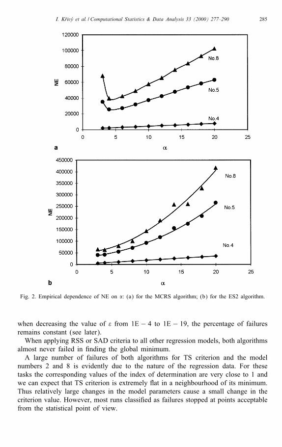
Fig. 2. Empirical dependence of NE on �: (a) for the MCRS algorithm; (b) for the ES2 algorithm.

when decreasing the value of � from 1E − 4 to 1E − 19, the percentage of failuresremains constant (see later).When applying RSS or SAD criteria to all other regression models, both algorithms

almost never failed in �nding the global minimum.A large number of failures of both algorithms for TS criterion and the model

numbers 2 and 8 is evidently due to the nature of the regression data. For thesetasks the corresponding values of the index of determination are very close to 1 andwe can expect that TS criterion is extremely at in a neighbourhood of its minimum.Thus relatively large changes in the model parameters cause a small change in thecriterion value. However, most runs classi�ed as failures stopped at points acceptablefrom the statistical point of view.


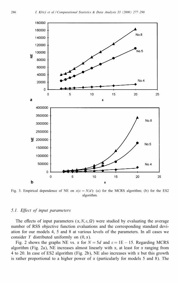
Fig. 3. Empirical dependence of NE on x(x = N=d): (a) for the MCRS algorithm; (b) for the ES2algorithm.

5.1. E�ect of input parameters

The e�ects of input parameters (�; N; �; ) were studied by evaluating the averagenumber of RSS objective function evaluations and the corresponding standard devi-ation for our models 4, 5 and 8 at various levels of the parameters. In all cases weconsider Y distributed uniformly on (0; �).Fig. 2 shows the graphs NE vs. � for N =5d and �=1E− 15. Regarding MCRS

algorithm (Fig. 2a), NE increases almost linearly with �, at least for � ranging from4 to 20. In case of ES2 algorithm (Fig. 2b), NE also increases with � but this growthis rather proportional to a higher power of � (particularly for models 5 and 8). The


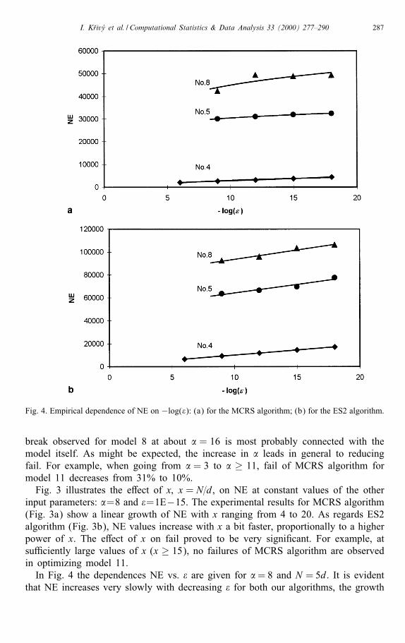
Fig. 4. Empirical dependence of NE on −log(�): (a) for the MCRS algorithm; (b) for the ES2 algorithm.

break observed for model 8 at about � = 16 is most probably connected with themodel itself. As might be expected, the increase in � leads in general to reducingfail. For example, when going from � = 3 to � ≥ 11, fail of MCRS algorithm formodel 11 decreases from 31% to 10%.Fig. 3 illustrates the e�ect of x; x = N=d, on NE at constant values of the other

input parameters: �=8 and �=1E−15. The experimental results for MCRS algorithm(Fig. 3a) show a linear growth of NE with x ranging from 4 to 20. As regards ES2algorithm (Fig. 3b), NE values increase with x a bit faster, proportionally to a higherpower of x. The e�ect of x on fail proved to be very signi�cant. For example, atsu�ciently large values of x (x ≥ 15), no failures of MCRS algorithm are observedin optimizing model 11.In Fig. 4 the dependences NE vs. � are given for �= 8 and N = 5d. It is evident

that NE increases very slowly with decreasing � for both our algorithms, the growth


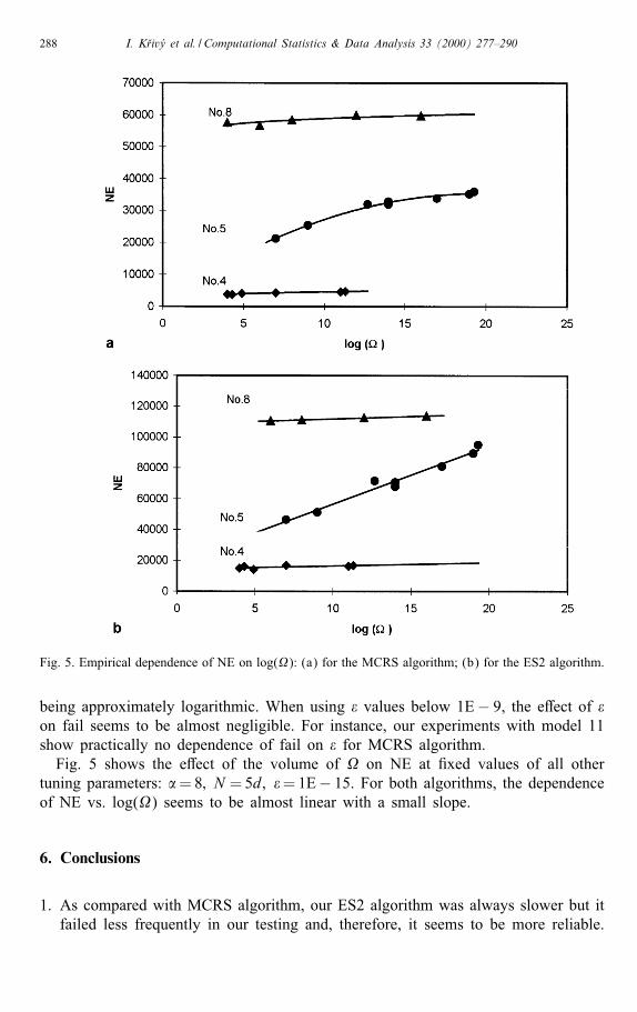
Fig. 5. Empirical dependence of NE on log(): (a) for the MCRS algorithm; (b) for the ES2 algorithm.

being approximately logarithmic. When using � values below 1E− 9, the e�ect of �on fail seems to be almost negligible. For instance, our experiments with model 11show practically no dependence of fail on � for MCRS algorithm.Fig. 5 shows the e�ect of the volume of on NE at �xed values of all other

tuning parameters: �=8; N =5d; �=1E− 15. For both algorithms, the dependenceof NE vs. log() seems to be almost linear with a small slope.

6. Conclusions

1. As compared with MCRS algorithm, our ES2 algorithm was always slower but itfailed less frequently in our testing and, therefore, it seems to be more reliable.


Our experiments (Tvrd��k and K�riv�y, 1995) proved that the relative robustnessof ES2 over MCRS cannot be attributed only to the larger NE performed byES2.

2. From the data in Table 2 it is evident that both our algorithms are signi�cantlymore reliable when compared with the optimizing algorithms built in standard sta-tistical packages. The algorithms can be also useful for solving more complicatedtasks in practice such as shape optimization (Haslinger et al., 1999), time-seriesanalysis, setting of knowledge networks, etc.

3. When using RSS or SAD optimization criteria, the algorithms are also su�cientlyreliable regarding the percentage of failures. The failure rate can be considerablyreduced by proper setting of its input parameters.

4. It is expected that a further increase in the reliability of the algorithms can beachieved by adding new points to increase N or by interchanging a few di�erentsearching algorithms during the optimization process.

Acknowledgements

This work was supported in part by a research grant No. 402=96=0823 from theGrant Agency of the Czech Republic.

References

Ali, M.M., T�orn, A., Viitanen, S., 1997. A numerical comparison of some controlled random searchalgorithms. J. Global Optim. 11, 377–385.

Conlon, M., 1992. The controlled random search procedure for function optimization. Commun.Statist.-Simula. Comput. 21, 919–923.

Goldberg, D.E., 1989. Genetic Algorithms in Search, Optimization, and Machine Learning.Addison-Wesley, Reading, MA.

Haslinger, J., Jedelsk�y, D., Kozubek, T., Tvrd��k, J., 1999. Genetic and random search methods inoptimal shape design problems. J. Global Optim., to appear in 1999.

Jennrich, R.I., Sampson, P.F., 1968. Application of stepwise regression to non-linear estimation.Technometrics 10 (1), 63–72.

K�riv�y, I., Tvrd��k, J., 1995. The controlled random search algorithm in optimizing regression models.Comput. Statist. and Data Anal. 20, 229–234.

K�riv�y, I., Tvrd��k, J., 1996. Stochastic algorithms in estimating regression models. In: Prat, A. (Ed.),Compstat 96, Proceedings in Computational Statistics. Physica-Verlag, Heidelberg, pp. 325–330.

K�riv�y, I., Tvrd��k, J., 1997. Some evolutionary algorithms for optimization. In: O�smera, P. (Ed.),Proceedings of 3rd International Mendel Conference on Genetic Algorithms, Fuzzy Logic, NeuralNetworks, Rough Sets. PC-DIR, Brno, pp. 65–70.

Kvasni�cka, V., Posp��chal, J., 1997. A hybrid of simplex method and simulated annealing. ChemometricsIntell. Lab. Systems 39, 161–173.

Price, W.L., 1976. A controlled random search procedure for global optimisation. Comput. J. 20,367–370.

Meyer, R.R., Roth, P.M., 1972. Modi�ed damped least squares: an algorithm for non-linear estimation.J. Inst. Math. Appl. 9, 218–233.


Michalewicz, Z., 1992. Genetic Algorithms+Data Structures = Evolutionary Program. Springer, Berlin.Militk�y, J., Meloun, M., 1994. Modus operandi of the least squares algorithm MINOPT. Talanta 40(2), 269–277.

Militk�y, J., 1995. Private communication.Tvrd��k, J., K�riv�y, I., 1995. Stochastic algorithms in estimating regression parameters. In: Han�clov�a,J. (Ed.), Proceedings of the MME’95 Symposium. AIMES Press, Ostrava, pp. 217–228.

Documents

Stochastic algorithms in nonlinear regression