Stiffness scaling laws and vibration isolators

Stiffness scaling laws and vibration isolators

Leif Kari*

MWL/Department of Vehicle Engineering, Royal Institute of Technology, 100 44 Stockholm, Sweden

Received 28 February 2001; received in revised form 12 October 2001; accepted 23 October 2001

Abstract

The variation in dynamic stiffness due to a geometrical shift of a cylindrical vibration iso-

lator is predicted by a scaling law and compared to the results of a waveguide solution. Thesimple scaling law fails to model satisfactorily the stiffness variation due to a single length orradius shift, while predicting successfully the results of an isolator shape invariant shift. The

small deviations arise from a disregarded material property shift. # 2002 Elsevier ScienceLtd. All rights reserved.

1. Introduction

The preparation of this paper is prompted by the appearance, among engineers, ofsimple models to convert scale-model tests and to predict the geometrical stiffnessshift of a vibration isolator from a laboriously determined stiffness; for example,from a measurement or a finite element method result. The applied scaling law isbased on simple principles; for example, the dynamic stiffness is proportional to theisolator cross-section area, to the inverse of its length and that ‘when doubling theisolator length, the stiffness (anti)resonance frequencies are halved’. How does onego about convincing an engineer, or anybody else for that matter, that this scalinglaw is seriously defective? To this end, the rubber material is modeled as nearlyincompressible, with viscoelasticity based on a fractional order derivative model [1].The main advantage of the viscoelastic model is the minimum parameter numberrequired to model the material properties successfully over a broad structure bornesound frequency domain. The dynamic stiffness of a cylindrical reference isolator iscalculated by a waveguide model [2,3], where the eigenvalues and eigenmodes of the

Applied Acoustics 63 (2002) 583–594

www.elsevier.com/locate/apacoust

0003-682X/02/$ - see front matter # 2002 Elsevier Science Ltd. All rights reserved.

PI I : S0003-682X(01 )00068 -8

* Tel.: +46-8-7907974; fax: +46-8-7906122.

E-mail address: [email protected]

cylinder cross-section are calculated. The total field is obtained by an eigenmodesuperposition, matched to the cylinder end boundary conditions. The stiffness varia-tion due to a geometrical shift of the reference isolator is then predicted by a scalinglaw and compared to the results of a waveguide solution for the altered isolator.

2. Method

2.1. Test object

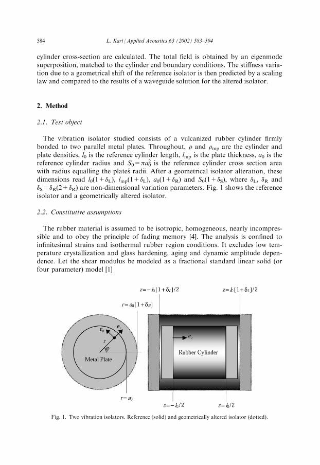
The vibration isolator studied consists of a vulcanized rubber cylinder firmlybonded to two parallel metal plates. Throughout, � and �mp are the cylinder andplate densities, l0 is the reference cylinder length, lmp is the plate thickness, a0 is thereference cylinder radius and S0=�a0

2 is the reference cylinder cross section areawith radius equalling the plates radii. After a geometrical isolator alteration, thesedimensions read l0(1+�L), lmp(1+�L), a0(1+�R) and S0(1+�S), where �L, �R and�S=�R(2+�R) are non-dimensional variation parameters. Fig. 1 shows the referenceisolator and a geometrically altered isolator.

2.2. Constitutive assumptions

The rubber material is assumed to be isotropic, homogeneous, nearly incompres-sible and to obey the principle of fading memory [4]. The analysis is confined toinfinitesimal strains and isothermal rubber region conditions. It excludes low tem-perature crystallization and glass hardening, aging and dynamic amplitude depen-dence. Let the shear modulus be modeled as a fractional standard linear solid (orfour parameter) model [1]

Fig. 1. Two vibration isolators. Reference (solid) and geometrically altered isolator (dotted).

584 L. Kari / Applied Acoustics 63 (2002) 583–594

�ð!Þ ¼ �1

1þ1þ�

�

�v

�1

i!

� ��

1þ1

�

�v

�1

i!

� �� ; ð1Þ

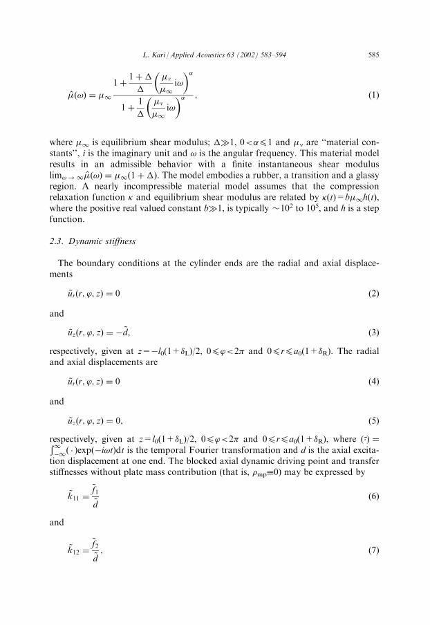
where �1 is equilibrium shear modulus; ��1, 0<�41 and �n are ‘‘material con-stants’’, i is the imaginary unit and ! is the angular frequency. This material modelresults in an admissible behavior with a finite instantaneous shear moduluslim! ! 1�ð!Þ ¼ �1ð1þ�Þ. The model embodies a rubber, a transition and a glassyregion. A nearly incompressible material model assumes that the compressionrelaxation function and equilibrium shear modulus are related by (t)=b�1h(t),where the positive real valued constant b�1, is typically �102 to 105, and h is a stepfunction.

2.3. Dynamic stiffness

The boundary conditions at the cylinder ends are the radial and axial displace-ments

u~rðr; ’; zÞ ¼ 0 ð2Þ

and

u~zðr; ’; zÞ ¼ d~; ð3Þ

respectively, given at z=l0(1+�L)/2, 04’<2� and 04r4a0(1+�R). The radialand axial displacements are

u~rðr; ’; zÞ ¼ 0 ð4Þ

and

u~zðr; ’; zÞ ¼ 0; ð5Þ

respectively, given at z=l0(1+�L)/2, 04’<2� and 04r4a0(1+�R), where ~ð Þ ¼Ð11

ð Þexpði!tÞdt is the temporal Fourier transformation and d is the axial excita-tion displacement at one end. The blocked axial dynamic driving point and transferstiffnesses without plate mass contribution (that is, �mp�0) may be expressed by

k~11 ¼f~1

d~ð6Þ

and

k~12 ¼f~2

d~; ð7Þ

L. Kari / Applied Acoustics 63 (2002) 583–594 585

where f1 and f2 are the axial tension force at the cylinder ends z=l0(1+�L)/2 andz=l0(1+�L)/2, respectively. To include the plate mass contribution, the drivingpoint stiffness in (6) is reduced by the plate mass times the square of the angularfrequency. The transfer stiffness, however, is independent of the plate mass.

2.4. Scaling law

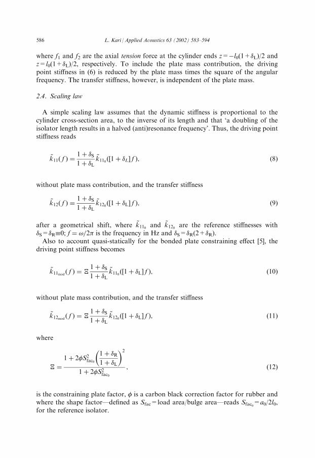
A simple scaling law assumes that the dynamic stiffness is proportional to thecylinder cross-section area, to the inverse of its length and that ‘a doubling of theisolator length results in a halved (anti)resonance frequency’. Thus, the driving pointstiffness reads

k~11ð f Þ ¼1þ �S1þ �L

k~110 ð½1þ �L f Þ; ð8Þ

without plate mass contribution, and the transfer stiffness

k~12ð f Þ ¼1þ �S1þ �L

k~120 ð½1þ �L f Þ; ð9Þ

after a geometrical shift, where k~110 and k~120 are the reference stiffnesses with�S=�R�0; f ¼ !=2� is the frequency in Hz and �S=�R(2+�R).Also to account quasi-statically for the bonded plate constraining effect [5], the

driving point stiffness becomes

k~11modð f Þ ¼ �

1þ �S1þ �L

k~110 ð½1þ �L f Þ; ð10Þ

without plate mass contribution, and the transfer stiffness

k~12modð f Þ ¼ �

1þ �S1þ �L

k~120 ð½1þ �L f Þ; ð11Þ

where

� ¼

1þ 2�S2fac01þ �R1þ �L

� �2

1þ 2�S2fac0; ð12Þ

is the constraining plate factor, � is a carbon black correction factor for rubber andwhere the shape factor—defined as Sfac=load area/bulge area—reads Sfac0=a0/2l0,for the reference isolator.


3. Results and discussion

3.1. Rubber material properties

The material parameters of Section 2.2 are: �=0.297, b=2.22 103, �1=5.94 105

N/m2, �n=5.99 Ns/m2 and �=1.05 103, kg/m3. The intensity � is undetermined as

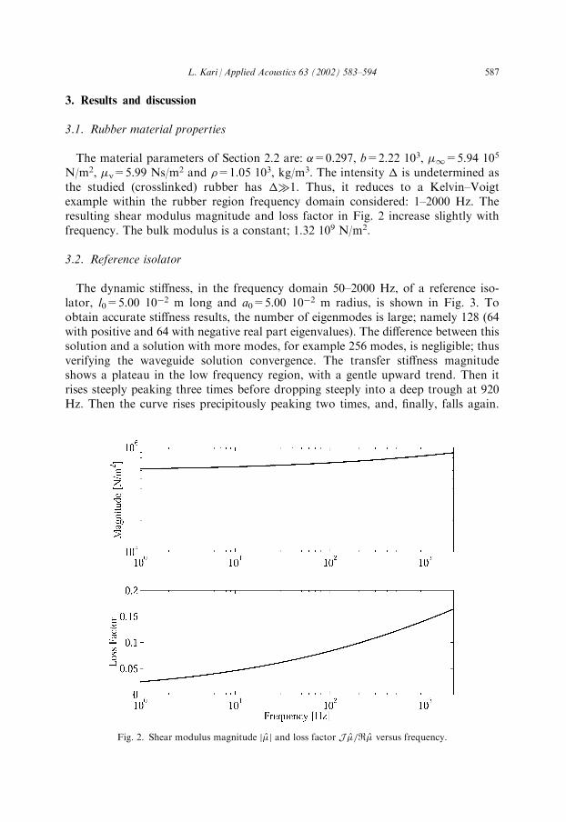
the studied (crosslinked) rubber has ��1. Thus, it reduces to a Kelvin–Voigtexample within the rubber region frequency domain considered: 1–2000 Hz. Theresulting shear modulus magnitude and loss factor in Fig. 2 increase slightly withfrequency. The bulk modulus is a constant; 1.32 109 N/m2.

3.2. Reference isolator

The dynamic stiffness, in the frequency domain 50–2000 Hz, of a reference iso-lator, l0=5.00 10

2 m long and a0=5.00 102 m radius, is shown in Fig. 3. To

obtain accurate stiffness results, the number of eigenmodes is large; namely 128 (64with positive and 64 with negative real part eigenvalues). The difference between thissolution and a solution with more modes, for example 256 modes, is negligible; thusverifying the waveguide solution convergence. The transfer stiffness magnitudeshows a plateau in the low frequency region, with a gentle upward trend. Then itrises steeply peaking three times before dropping steeply into a deep trough at 920Hz. Then the curve rises precipitously peaking two times, and, finally, falls again.

Fig. 2. Shear modulus magnitude �j j and loss factor J �=R� versus frequency.


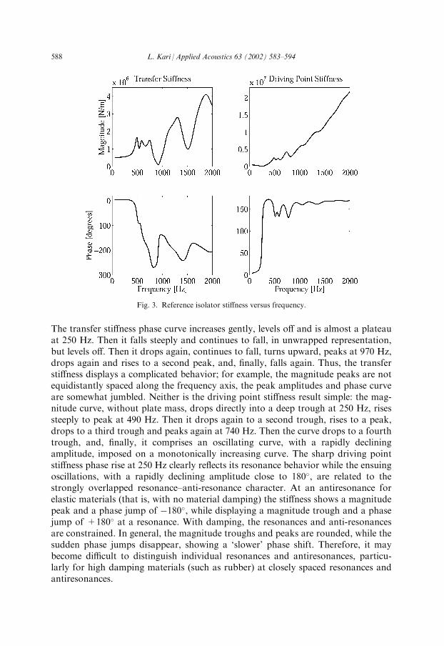
The transfer stiffness phase curve increases gently, levels off and is almost a plateauat 250 Hz. Then it falls steeply and continues to fall, in unwrapped representation,but levels off. Then it drops again, continues to fall, turns upward, peaks at 970 Hz,drops again and rises to a second peak, and, finally, falls again. Thus, the transferstiffness displays a complicated behavior; for example, the magnitude peaks are notequidistantly spaced along the frequency axis, the peak amplitudes and phase curveare somewhat jumbled. Neither is the driving point stiffness result simple: the mag-nitude curve, without plate mass, drops directly into a deep trough at 250 Hz, risessteeply to peak at 490 Hz. Then it drops again to a second trough, rises to a peak,drops to a third trough and peaks again at 740 Hz. Then the curve drops to a fourthtrough, and, finally, it comprises an oscillating curve, with a rapidly decliningamplitude, imposed on a monotonically increasing curve. The sharp driving pointstiffness phase rise at 250 Hz clearly reflects its resonance behavior while the ensuingoscillations, with a rapidly declining amplitude close to 180�, are related to thestrongly overlapped resonance–anti-resonance character. At an antiresonance forelastic materials (that is, with no material damping) the stiffness shows a magnitudepeak and a phase jump of 180�, while displaying a magnitude trough and a phasejump of +180� at a resonance. With damping, the resonances and anti-resonancesare constrained. In general, the magnitude troughs and peaks are rounded, while thesudden phase jumps disappear, showing a ‘slower’ phase shift. Therefore, it maybecome difficult to distinguish individual resonances and antiresonances, particu-larly for high damping materials (such as rubber) at closely spaced resonances andantiresonances.

Fig. 3. Reference isolator stiffness versus frequency.


3.3. Length variation results

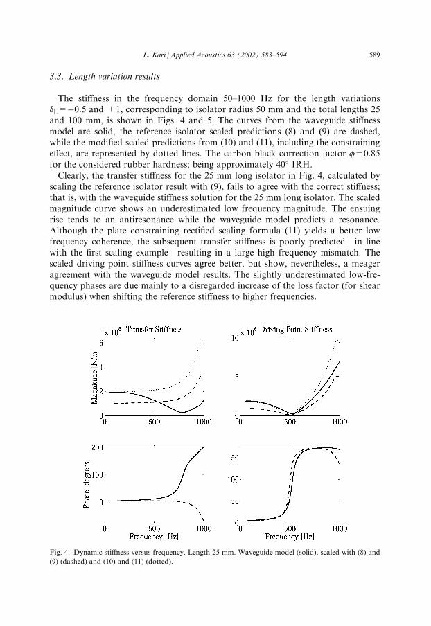
The stiffness in the frequency domain 50–1000 Hz for the length variations�L=0.5 and +1, corresponding to isolator radius 50 mm and the total lengths 25and 100 mm, is shown in Figs. 4 and 5. The curves from the waveguide stiffnessmodel are solid, the reference isolator scaled predictions (8) and (9) are dashed,while the modified scaled predictions from (10) and (11), including the constrainingeffect, are represented by dotted lines. The carbon black correction factor �=0.85for the considered rubber hardness; being approximately 40� IRH.Clearly, the transfer stiffness for the 25 mm long isolator in Fig. 4, calculated by

scaling the reference isolator result with (9), fails to agree with the correct stiffness;that is, with the waveguide stiffness solution for the 25 mm long isolator. The scaledmagnitude curve shows an underestimated low frequency magnitude. The ensuingrise tends to an antiresonance while the waveguide model predicts a resonance.Although the plate constraining rectified scaling formula (11) yields a better lowfrequency coherence, the subsequent transfer stiffness is poorly predicted—in linewith the first scaling example—resulting in a large high frequency mismatch. Thescaled driving point stiffness curves agree better, but show, nevertheless, a meageragreement with the waveguide model results. The slightly underestimated low-fre-quency phases are due mainly to a disregarded increase of the loss factor (for shearmodulus) when shifting the reference stiffness to higher frequencies.

Fig. 4. Dynamic stiffness versus frequency. Length 25 mm. Waveguide model (solid), scaled with (8) and

(9) (dashed) and (10) and (11) (dotted).


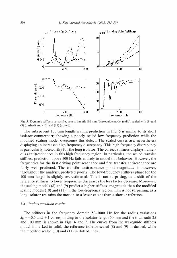
The subsequent 100 mm length scaling prediction in Fig. 5 is similar to its shortisolator counterpart; showing a poorly scaled low frequency prediction while themodified scaling model overcomes this defect. The scaled curves are, neverthelessdisplaying an increased high frequency discrepancy. This high frequency discrepancyis particularly noteworthy for the long isolator. The correct stiffness displays numer-ous (anti)resonances in this high frequency region. In particular, the scaled transferstiffness prediction above 500 Hz fails entirely to model this behavior. However, thefrequencies for the first driving point resonance and first transfer antiresonance arefairly well predicted. The transfer antiresonance point magnitude is however,throughout the analysis, predicted poorly. The low-frequency stiffness phase for the100 mm length is slightly overestimated. This is not surprising, as a shift of thereference stiffness to lower frequencies disregards the loss factor decrease. Moreover,the scaling models (8) and (9) predict a higher stiffness magnitude than the modifiedscaling models (10) and (11), in the low-frequency region. This is not surprising, as along isolator restrains the motion to a lesser extent than a shorter reference.

3.4. Radius variation results

The stiffness in the frequency domain 50–1000 Hz for the radius variations�R=0.5 and +1 corresponding to the isolator length 50 mm and the total radii 25and 100 mm, is shown in Figs. 6 and 7. The curves from the waveguide stiffnessmodel is marked in solid, the reference isolator scaled (8) and (9) in dashed, whilethe modified scaled (10) and (11) in dotted lines.

Fig. 5. Dynamic stiffness versus frequency. Length 100 mm. Waveguide model (solid), scaled with (8) and



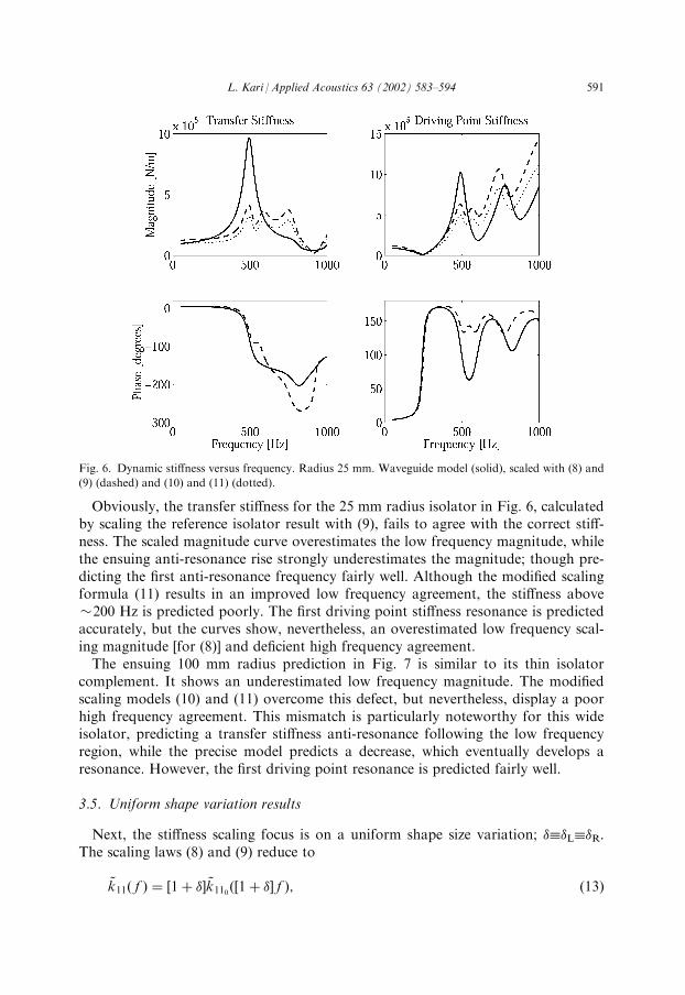
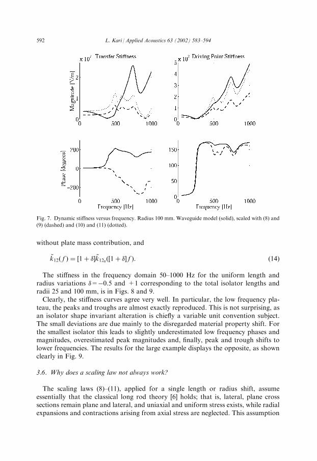
Obviously, the transfer stiffness for the 25 mm radius isolator in Fig. 6, calculatedby scaling the reference isolator result with (9), fails to agree with the correct stiff-ness. The scaled magnitude curve overestimates the low frequency magnitude, whilethe ensuing anti-resonance rise strongly underestimates the magnitude; though pre-dicting the first anti-resonance frequency fairly well. Although the modified scalingformula (11) results in an improved low frequency agreement, the stiffness above�200 Hz is predicted poorly. The first driving point stiffness resonance is predictedaccurately, but the curves show, nevertheless, an overestimated low frequency scal-ing magnitude [for (8)] and deficient high frequency agreement.The ensuing 100 mm radius prediction in Fig. 7 is similar to its thin isolator

complement. It shows an underestimated low frequency magnitude. The modifiedscaling models (10) and (11) overcome this defect, but nevertheless, display a poorhigh frequency agreement. This mismatch is particularly noteworthy for this wideisolator, predicting a transfer stiffness anti-resonance following the low frequencyregion, while the precise model predicts a decrease, which eventually develops aresonance. However, the first driving point resonance is predicted fairly well.

3.5. Uniform shape variation results

Next, the stiffness scaling focus is on a uniform shape size variation; ��L��R.The scaling laws (8) and (9) reduce to

k~11ð f Þ ¼ ½1þ � k~110ð½1þ � f Þ; ð13Þ

Fig. 6. Dynamic stiffness versus frequency. Radius 25 mm. Waveguide model (solid), scaled with (8) and



without plate mass contribution, and

k~12ð f Þ ¼ ½1þ � k~120ð½1þ � f Þ: ð14Þ

The stiffness in the frequency domain 50–1000 Hz for the uniform length andradius variations �=0.5 and +1 corresponding to the total isolator lengths andradii 25 and 100 mm, is in Figs. 8 and 9.Clearly, the stiffness curves agree very well. In particular, the low frequency pla-

teau, the peaks and troughs are almost exactly reproduced. This is not surprising, asan isolator shape invariant alteration is chiefly a variable unit convention subject.The small deviations are due mainly to the disregarded material property shift. Forthe smallest isolator this leads to slightly underestimated low frequency phases andmagnitudes, overestimated peak magnitudes and, finally, peak and trough shifts tolower frequencies. The results for the large example displays the opposite, as shownclearly in Fig. 9.

3.6. Why does a scaling law not always work?

The scaling laws (8)–(11), applied for a single length or radius shift, assumeessentially that the classical long rod theory [6] holds; that is, lateral, plane crosssections remain plane and lateral, and uniaxial and uniform stress exists, while radialexpansions and contractions arising from axial stress are neglected. This assumption

Fig. 7. Dynamic stiffness versus frequency. Radius 100 mm. Waveguide model (solid), scaled with (8) and



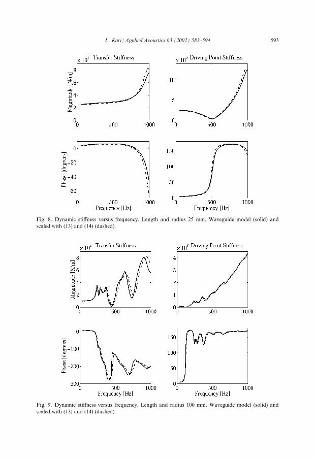
Fig. 8. Dynamic stiffness versus frequency. Length and radius 25 mm. Waveguide model (solid) and

scaled with (13) and (14) (dashed).

Fig. 9. Dynamic stiffness versus frequency. Length and radius 100 mm. Waveguide model (solid) and

scaled with (13) and (14) (dashed).


is not correct [3]—paricularly not for large diameter-to-length ratios (present case).The increased influence of dispersion and the increased influence of higher ordermodes, required for satisfaction of the boundary conditions (2)–(5), explain the dis-crepancies reported for the approximate theory. The scaling laws (13) and (14) foran isolator shape invariant shift is, however, mainly a variable unit conventionsubject—an observation fully consistent with Rayleigh [7]. The small deviationsarise from a disregarded material property shift.

4. Conclusions

It is found that a simple scaling law fails to predict the isolator stiffness alterationdue to a single length or radius shift, while successfully modeling the results of anisolator shape invariant shift. The small deviations for the latter case—for example,minor stiffness trough and peak shifts, slightly under- or overestimated low-fre-quency stiffness magnitudes and phases—arise from a disregarded material propertyshift. The large discrepancies reported for a single length or radius shift are duemainly to an incorrect scaling law hypothesis.Essentially this is the result of assuming that lateral, plane cross sections remain

plane and lateral, and uniaxial and uniform stress exists, while radial expansions andcontractions arising from axial stress are neglected. This classical long rod model isnot correct for ordinary rubber isolators. The increased influence of higher ordermodes, required for satisfaction of the displacement boundary conditions at thebonded ends of the isolator, and the increased influence of dispersion, explain thediscrepancies reported for the approximate theory.An interesting continuation of the work presented is to find a, not too laborious,

scaling law which is able to accurately predict the stiffness variation due to a singlelength or radius shift of the isolator.

References

[1] Bagley RL, Torvik PJ. Fractional calculus—a different approach to the analysis of viscoelastically

damped structures. AIAA Journal 1983;21:741–8.

[2] Kari L. On the waveguide modelling of dynamic stiffness of cylindrical vibration isolators. Part I: the

model, solution and experimental comparison. Journal of Sound and Vibration 2001;244:211–33.

[3] Kari L. On the waveguide modelling of dynamic stiffness of cylindrical vibration isolators. Part II:

the dispersion relation solution, convergence analysis and comparison with simple models. Journal of

Sound and Vibration 2001;244:235–57.

[4] Christensen RM. Theory of viscoelasticity. 2nd ed. New York: Academic Press, 1982.

[5] Gent AN. Engineering with rubber. Munich: Carl Hanser, 1992.

[6] Snowdon JC. Vibration and shock in damped mechanical systems. New York: John Wiley & Sons,

1968.

[7] Rayleigh JWS. The theory of sound. 2nd ed. New York: Dover Publications, 1945.


Documents

Stiffness scaling laws and vibration isolators