Embed Size (px)
Citation preview

StevenShreve: StochasticCalculusandFinance
PRASAD CHALASANI
CarnegieMellon [email protected]
SOMESH JHA
CarnegieMellon [email protected]
THIS IS A DRAFT: PLEASEDO NOT DISTRIBUTEc
Copyright;StevenE. Shreve,1996
October6, 1997
Contents
1 Intr oduction to Probability Theory 11
1.1 TheBinomialAssetPricingModel . . . . . . . . . . . . . . . . . . . . . . . . . . 11
1.2 FiniteProbabilitySpaces. . . . . . . . . . . . . . . . . . . . . . . . . . . . . . . 16
1.3 LebesgueMeasureandtheLebesgueIntegral . . . . . . . . . . . . . . . . . . . . 22
1.4 GeneralProbabilitySpaces. . . . . . . . . . . . . . . . . . . . . . . . . . . . . . 30
1.5 Independence. . . . . . . . . . . . . . . . . . . . . . . . . . . . . . . . . . . . . 40
1.5.1 Independenceof sets . . . . . . . . . . . . . . . . . . . . . . . . . . . . . 40
1.5.2 Independenceof -algebras . . . . . . . . . . . . . . . . . . . . . . . . . 41
1.5.3 Independenceof randomvariables. . . . . . . . . . . . . . . . . . . . . . 42
1.5.4 Correlationandindependence. . . . . . . . . . . . . . . . . . . . . . . . 44
1.5.5 Independenceandconditionalexpectation. . . . . . . . . . . . . . . . . . 45
1.5.6 Law of LargeNumbers. . . . . . . . . . . . . . . . . . . . . . . . . . . . 46
1.5.7 CentralLimit Theorem. . . . . . . . . . . . . . . . . . . . . . . . . . . . 47
2 Conditional Expectation 49
2.1 A BinomialModel for StockPriceDynamics . . . . . . . . . . . . . . . . . . . . 49
2.2 Information . . . . . . . . . . . . . . . . . . . . . . . . . . . . . . . . . . . . . . 50
2.3 ConditionalExpectation . . . . . . . . . . . . . . . . . . . . . . . . . . . . . . . 52
2.3.1 An example . . . . . . . . . . . . . . . . . . . . . . . . . . . . . . . . . . 52
2.3.2 Definitionof ConditionalExpectation . . . . . . . . . . . . . . . . . . . . 53
2.3.3 Furtherdiscussionof Partial Averaging . . . . . . . . . . . . . . . . . . . 54
2.3.4 Propertiesof ConditionalExpectation . . . . . . . . . . . . . . . . . . . . 55
2.3.5 Examplesfrom theBinomialModel . . . . . . . . . . . . . . . . . . . . . 57
2.4 Martingales . . . . . . . . . . . . . . . . . . . . . . . . . . . . . . . . . . . . . . 58
1
2
3 Arbitrage Pricing 59
3.1 BinomialPricing . . . . . . . . . . . . . . . . . . . . . . . . . . . . . . . . . . . 59
3.2 Generalone-stepAPT . . . . . . . . . . . . . . . . . . . . . . . . . . . . . . . . . 60
3.3 Risk-NeutralProbabilityMeasure . . . . . . . . . . . . . . . . . . . . . . . . . . 61
3.3.1 PortfolioProcess. . . . . . . . . . . . . . . . . . . . . . . . . . . . . . . 62
3.3.2 Self-financingValueof a PortfolioProcess . . . . . . . . . . . . . . . . 62
3.4 SimpleEuropeanDerivativeSecurities. . . . . . . . . . . . . . . . . . . . . . . . 63
3.5 TheBinomialModel is Complete. . . . . . . . . . . . . . . . . . . . . . . . . . . 64
4 The Mark ov Property 67
4.1 BinomialModelPricingandHedging . . . . . . . . . . . . . . . . . . . . . . . . 67
4.2 ComputationalIssues. . . . . . . . . . . . . . . . . . . . . . . . . . . . . . . . . 69
4.3 Markov Processes. . . . . . . . . . . . . . . . . . . . . . . . . . . . . . . . . . . 70
4.3.1 Differentwaysto write theMarkov property . . . . . . . . . . . . . . . . 70
4.4 Showing thata processis Markov . . . . . . . . . . . . . . . . . . . . . . . . . . 73
4.5 Applicationto ExoticOptions . . . . . . . . . . . . . . . . . . . . . . . . . . . . 74
5 StoppingTimesand American Options 77
5.1 AmericanPricing . . . . . . . . . . . . . . . . . . . . . . . . . . . . . . . . . . . 77
5.2 Valueof PortfolioHedginganAmericanOption . . . . . . . . . . . . . . . . . . . 79
5.3 Informationup to aStoppingTime . . . . . . . . . . . . . . . . . . . . . . . . . . 81
6 Propertiesof American Derivative Securities 85
6.1 Theproperties. . . . . . . . . . . . . . . . . . . . . . . . . . . . . . . . . . . . . 85
6.2 Proofsof theProperties. . . . . . . . . . . . . . . . . . . . . . . . . . . . . . . . 86
6.3 CompoundEuropeanDerivativeSecurities. . . . . . . . . . . . . . . . . . . . . . 88
6.4 OptimalExerciseof AmericanDerivativeSecurity. . . . . . . . . . . . . . . . . . 89
7 Jensen’s Inequality 91
7.1 Jensen’s Inequalityfor ConditionalExpectations. . . . . . . . . . . . . . . . . . . 91
7.2 OptimalExerciseof anAmericanCall . . . . . . . . . . . . . . . . . . . . . . . . 92
7.3 StoppedMartingales . . . . . . . . . . . . . . . . . . . . . . . . . . . . . . . . . 94
8 RandomWalks 97
8.1 FirstPassageTime . . . . . . . . . . . . . . . . . . . . . . . . . . . . . . . . . . 97
3
8.2 is almostsurelyfinite . . . . . . . . . . . . . . . . . . . . . . . . . . . . . . . . 97
8.3 Themomentgeneratingfunctionfor . . . . . . . . . . . . . . . . . . . . . . . . 99
8.4 Expectationof . . . . . . . . . . . . . . . . . . . . . . . . . . . . . . . . . . . . 100
8.5 TheStrongMarkov Property . . . . . . . . . . . . . . . . . . . . . . . . . . . . . 101
8.6 GeneralFirstPassageTimes . . . . . . . . . . . . . . . . . . . . . . . . . . . . . 101
8.7 Example:PerpetualAmericanPut . . . . . . . . . . . . . . . . . . . . . . . . . . 102
8.8 DifferenceEquation. . . . . . . . . . . . . . . . . . . . . . . . . . . . . . . . . . 106
8.9 Distributionof FirstPassageTimes . . . . . . . . . . . . . . . . . . . . . . . . . . 107
8.10 TheReflectionPrinciple . . . . . . . . . . . . . . . . . . . . . . . . . . . . . . . 109
9 Pricing in terms of Market Probabilities: The Radon-Nikodym Theorem. 111
9.1 Radon-NikodymTheorem . . . . . . . . . . . . . . . . . . . . . . . . . . . . . . 111
9.2 Radon-NikodymMartingales. . . . . . . . . . . . . . . . . . . . . . . . . . . . . 112
9.3 TheStatePriceDensityProcess . . . . . . . . . . . . . . . . . . . . . . . . . . . 113
9.4 StochasticVolatility BinomialModel . . . . . . . . . . . . . . . . . . . . . . . . . 116
9.5 AnotherApplicatonof theRadon-NikodymTheorem . . . . . . . . . . . . . . . . 118
10 Capital AssetPricing 119
10.1 An OptimizationProblem. . . . . . . . . . . . . . . . . . . . . . . . . . . . . . . 119
11 GeneralRandomVariables 123
11.1 Law of a RandomVariable . . . . . . . . . . . . . . . . . . . . . . . . . . . . . . 123
11.2 Densityof aRandomVariable . . . . . . . . . . . . . . . . . . . . . . . . . . . . 123
11.3 Expectation . . . . . . . . . . . . . . . . . . . . . . . . . . . . . . . . . . . . . . 124
11.4 Two randomvariables. . . . . . . . . . . . . . . . . . . . . . . . . . . . . . . . . 125
11.5 Marginal Density . . . . . . . . . . . . . . . . . . . . . . . . . . . . . . . . . . . 126
11.6 ConditionalExpectation . . . . . . . . . . . . . . . . . . . . . . . . . . . . . . . 126
11.7 ConditionalDensity . . . . . . . . . . . . . . . . . . . . . . . . . . . . . . . . . . 127
11.8 MultivariateNormalDistribution . . . . . . . . . . . . . . . . . . . . . . . . . . . 129
11.9 Bivariatenormaldistribution . . . . . . . . . . . . . . . . . . . . . . . . . . . . . 130
11.10MGF of jointly normalrandomvariables. . . . . . . . . . . . . . . . . . . . . . . 130
12 Semi-ContinuousModels 131
12.1 Discrete-timeBrownianMotion . . . . . . . . . . . . . . . . . . . . . . . . . . . 131
4
12.2 TheStockPriceProcess. . . . . . . . . . . . . . . . . . . . . . . . . . . . . . . . 132
12.3 Remainderof theMarket . . . . . . . . . . . . . . . . . . . . . . . . . . . . . . . 133
12.4 Risk-NeutralMeasure. . . . . . . . . . . . . . . . . . . . . . . . . . . . . . . . . 133
12.5 Risk-NeutralPricing . . . . . . . . . . . . . . . . . . . . . . . . . . . . . . . . . 134
12.6 Arbitrage . . . . . . . . . . . . . . . . . . . . . . . . . . . . . . . . . . . . . . . 134
12.7 StalkingtheRisk-NeutralMeasure. . . . . . . . . . . . . . . . . . . . . . . . . . 135
12.8 Pricinga EuropeanCall . . . . . . . . . . . . . . . . . . . . . . . . . . . . . . . . 138
13 Brownian Motion 139
13.1 SymmetricRandomWalk . . . . . . . . . . . . . . . . . . . . . . . . . . . . . . . 139
13.2 TheLaw of LargeNumbers. . . . . . . . . . . . . . . . . . . . . . . . . . . . . . 139
13.3 CentralLimit Theorem . . . . . . . . . . . . . . . . . . . . . . . . . . . . . . . . 140
13.4 BrownianMotion asaLimit of RandomWalks . . . . . . . . . . . . . . . . . . . 141
13.5 BrownianMotion . . . . . . . . . . . . . . . . . . . . . . . . . . . . . . . . . . . 142
13.6 Covarianceof BrownianMotion . . . . . . . . . . . . . . . . . . . . . . . . . . . 143
13.7 Finite-DimensionalDistributionsof BrownianMotion . . . . . . . . . . . . . . . . 144
13.8 Filtrationgeneratedby a BrownianMotion . . . . . . . . . . . . . . . . . . . . . . 144
13.9 MartingaleProperty. . . . . . . . . . . . . . . . . . . . . . . . . . . . . . . . . . 145
13.10TheLimit of a BinomialModel . . . . . . . . . . . . . . . . . . . . . . . . . . . . 145
13.11StartingatPointsOtherThan0 . . . . . . . . . . . . . . . . . . . . . . . . . . . . 147
13.12Markov Propertyfor BrownianMotion . . . . . . . . . . . . . . . . . . . . . . . . 147
13.13TransitionDensity. . . . . . . . . . . . . . . . . . . . . . . . . . . . . . . . . . . 149
13.14FirstPassageTime . . . . . . . . . . . . . . . . . . . . . . . . . . . . . . . . . . 149
14 The It o Integral 153
14.1 BrownianMotion . . . . . . . . . . . . . . . . . . . . . . . . . . . . . . . . . . . 153
14.2 FirstVariation . . . . . . . . . . . . . . . . . . . . . . . . . . . . . . . . . . . . . 153
14.3 QuadraticVariation . . . . . . . . . . . . . . . . . . . . . . . . . . . . . . . . . . 155
14.4 QuadraticVariationasAbsoluteVolatility . . . . . . . . . . . . . . . . . . . . . . 157
14.5 Constructionof theIto Integral . . . . . . . . . . . . . . . . . . . . . . . . . . . . 158
14.6 Ito integralof anelementaryintegrand . . . . . . . . . . . . . . . . . . . . . . . . 158
14.7 Propertiesof theIto integralof anelementaryprocess. . . . . . . . . . . . . . . . 159
14.8 Ito integralof a generalintegrand. . . . . . . . . . . . . . . . . . . . . . . . . . . 162
5
14.9 Propertiesof the(general)Ito integral . . . . . . . . . . . . . . . . . . . . . . . . 163
14.10Quadraticvariationof anIto integral . . . . . . . . . . . . . . . . . . . . . . . . . 165
15 It o’sFormula 167
15.1 Ito’s formulafor oneBrownianmotion . . . . . . . . . . . . . . . . . . . . . . . . 167
15.2 Derivationof Ito’s formula . . . . . . . . . . . . . . . . . . . . . . . . . . . . . . 168
15.3 GeometricBrownianmotion . . . . . . . . . . . . . . . . . . . . . . . . . . . . . 169
15.4 Quadraticvariationof geometricBrownianmotion . . . . . . . . . . . . . . . . . 170
15.5 Volatility of GeometricBrownianmotion . . . . . . . . . . . . . . . . . . . . . . 170
15.6 Firstderivationof theBlack-Scholesformula . . . . . . . . . . . . . . . . . . . . 170
15.7 Meanandvarianceof theCox-Ingersoll-Rossprocess. . . . . . . . . . . . . . . . 172
15.8 MultidimensionalBrownianMotion . . . . . . . . . . . . . . . . . . . . . . . . . 173
15.9 Cross-variationsof Brownianmotions . . . . . . . . . . . . . . . . . . . . . . . . 174
15.10Multi-dimensionalIto formula . . . . . . . . . . . . . . . . . . . . . . . . . . . . 175
16 Mark ov processesand the Kolmogorov equations 177
16.1 StochasticDif ferentialEquations. . . . . . . . . . . . . . . . . . . . . . . . . . . 177
16.2 Markov Property . . . . . . . . . . . . . . . . . . . . . . . . . . . . . . . . . . . 178
16.3 Transitiondensity . . . . . . . . . . . . . . . . . . . . . . . . . . . . . . . . . . . 179
16.4 TheKolmogorov BackwardEquation . . . . . . . . . . . . . . . . . . . . . . . . 180
16.5 ConnectionbetweenstochasticcalculusandKBE . . . . . . . . . . . . . . . . . . 181
16.6 Black-Scholes. . . . . . . . . . . . . . . . . . . . . . . . . . . . . . . . . . . . . 183
16.7 Black-Scholeswith price-dependentvolatility . . . . . . . . . . . . . . . . . . . . 186
17 Girsanov’s theorem and the risk-neutral measure 189
17.1 Conditionalexpectationsunder . . . . . . . . . . . . . . . . . . . . . . . . . . 191
17.2 Risk-neutralmeasure. . . . . . . . . . . . . . . . . . . . . . . . . . . . . . . . . 193
18 Martingale RepresentationTheorem 197
18.1 MartingaleRepresentationTheorem . . . . . . . . . . . . . . . . . . . . . . . . . 197
18.2 A hedgingapplication. . . . . . . . . . . . . . . . . . . . . . . . . . . . . . . . . 197
18.3 -dimensionalGirsanov Theorem . . . . . . . . . . . . . . . . . . . . . . . . . . 199
18.4 -dimensionalMartingaleRepresentationTheorem . . . . . . . . . . . . . . . . . 200
18.5 Multi-dimensionalmarketmodel . . . . . . . . . . . . . . . . . . . . . . . . . . . 200
6
19 A two-dimensionalmarket model 203
19.1 Hedgingwhen . . . . . . . . . . . . . . . . . . . . . . . . . . . . . . 204
19.2 Hedgingwhen . . . . . . . . . . . . . . . . . . . . . . . . . . . . . . . . . 205
20 Pricing Exotic Options 209
20.1 Reflectionprinciplefor Brownianmotion . . . . . . . . . . . . . . . . . . . . . . 209
20.2 Up andoutEuropeancall. . . . . . . . . . . . . . . . . . . . . . . . . . . . . . . 212
20.3 A practicalissue. . . . . . . . . . . . . . . . . . . . . . . . . . . . . . . . . . . . 218
21 Asian Options 219
21.1 Feynman-KacTheorem. . . . . . . . . . . . . . . . . . . . . . . . . . . . . . . . 220
21.2 Constructingthehedge . . . . . . . . . . . . . . . . . . . . . . . . . . . . . . . . 220
21.3 Partial averagepayoff Asianoption . . . . . . . . . . . . . . . . . . . . . . . . . . 221
22 Summary of Arbitrage Pricing Theory 223
22.1 Binomialmodel,HedgingPortfolio . . . . . . . . . . . . . . . . . . . . . . . . . 223
22.2 Settingup thecontinuousmodel . . . . . . . . . . . . . . . . . . . . . . . . . . . 225
22.3 Risk-neutralpricingandhedging . . . . . . . . . . . . . . . . . . . . . . . . . . . 227
22.4 Implementationof risk-neutralpricingandhedging . . . . . . . . . . . . . . . . . 229
23 Recognizinga Brownian Motion 233
23.1 Identifyingvolatility andcorrelation . . . . . . . . . . . . . . . . . . . . . . . . . 235
23.2 Reversingtheprocess. . . . . . . . . . . . . . . . . . . . . . . . . . . . . . . . . 236
24 An outsidebarrier option 239
24.1 Computingtheoptionvalue. . . . . . . . . . . . . . . . . . . . . . . . . . . . . . 242
24.2 ThePDEfor theoutsidebarrieroption . . . . . . . . . . . . . . . . . . . . . . . . 243
24.3 Thehedge. . . . . . . . . . . . . . . . . . . . . . . . . . . . . . . . . . . . . . . 245
25 American Options 247
25.1 Preview of perpetualAmericanput . . . . . . . . . . . . . . . . . . . . . . . . . . 247
25.2 Firstpassagetimesfor Brownianmotion:first method. . . . . . . . . . . . . . . . 247
25.3 Drift adjustment. . . . . . . . . . . . . . . . . . . . . . . . . . . . . . . . . . . . 249
25.4 Drift-adjustedLaplacetransform . . . . . . . . . . . . . . . . . . . . . . . . . . . 250
25.5 Firstpassagetimes:Secondmethod . . . . . . . . . . . . . . . . . . . . . . . . . 251
7
25.6 PerpetualAmericanput . . . . . . . . . . . . . . . . . . . . . . . . . . . . . . . . 252
25.7 Valueof theperpetualAmericanput . . . . . . . . . . . . . . . . . . . . . . . . . 256
25.8 Hedgingtheput . . . . . . . . . . . . . . . . . . . . . . . . . . . . . . . . . . . . 257
25.9 PerpetualAmericancontingentclaim . . . . . . . . . . . . . . . . . . . . . . . . . 259
25.10PerpetualAmericancall . . . . . . . . . . . . . . . . . . . . . . . . . . . . . . . . 259
25.11Putwith expiration . . . . . . . . . . . . . . . . . . . . . . . . . . . . . . . . . . 260
25.12Americancontingentclaimwith expiration . . . . . . . . . . . . . . . . . . . . . 261
26 Options on dividend-paying stocks 263
26.1 Americanoptionwith convex payoff function . . . . . . . . . . . . . . . . . . . . 263
26.2 Dividendpayingstock . . . . . . . . . . . . . . . . . . . . . . . . . . . . . . . . 264
26.3 Hedgingat time . . . . . . . . . . . . . . . . . . . . . . . . . . . . . . . . . . 266
27 Bonds,forward contractsand futur es 267
27.1 Forwardcontracts. . . . . . . . . . . . . . . . . . . . . . . . . . . . . . . . . . . 269
27.2 Hedginga forwardcontract. . . . . . . . . . . . . . . . . . . . . . . . . . . . . . 269
27.3 Futurecontracts. . . . . . . . . . . . . . . . . . . . . . . . . . . . . . . . . . . . 270
27.4 Cashflow from afuturecontract . . . . . . . . . . . . . . . . . . . . . . . . . . . 272
27.5 Forward-futurespread. . . . . . . . . . . . . . . . . . . . . . . . . . . . . . . . . 272
27.6 Backwardationandcontango. . . . . . . . . . . . . . . . . . . . . . . . . . . . . 273
28 Term-structure models 275
28.1 Computingarbitrage-freebondprices:first method . . . . . . . . . . . . . . . . . 276
28.2 Someinterest-ratedependentassets . . . . . . . . . . . . . . . . . . . . . . . . . 276
28.3 Terminology. . . . . . . . . . . . . . . . . . . . . . . . . . . . . . . . . . . . . . 277
28.4 Forwardrateagreement. . . . . . . . . . . . . . . . . . . . . . . . . . . . . . . . 277
28.5 Recoveringtheinterest from theforwardrate . . . . . . . . . . . . . . . . . . 278
28.6 Computingarbitrage-freebondprices:Heath-Jarrow-Mortonmethod. . . . . . . . 279
28.7 Checkingfor absenceof arbitrage . . . . . . . . . . . . . . . . . . . . . . . . . . 280
28.8 Implementationof theHeath-Jarrow-Mortonmodel . . . . . . . . . . . . . . . . . 281
29 Gaussianprocesses 285
29.1 An example:BrownianMotion . . . . . . . . . . . . . . . . . . . . . . . . . . . . 286
30 Hull and White model 293
8
30.1 Fiddlingwith theformulas . . . . . . . . . . . . . . . . . . . . . . . . . . . . . . 295
30.2 Dynamicsof thebondprice . . . . . . . . . . . . . . . . . . . . . . . . . . . . . . 296
30.3 Calibrationof theHull & Whitemodel . . . . . . . . . . . . . . . . . . . . . . . . 297
30.4 Optionona bond . . . . . . . . . . . . . . . . . . . . . . . . . . . . . . . . . . . 299
31 Cox-Ingersoll-Rossmodel 303
31.1 Equilibriumdistributionof . . . . . . . . . . . . . . . . . . . . . . . . . . . . 306
31.2 Kolmogorov forwardequation . . . . . . . . . . . . . . . . . . . . . . . . . . . . 306
31.3 Cox-Ingersoll-Rossequilibriumdensity . . . . . . . . . . . . . . . . . . . . . . . 309
31.4 Bondpricesin theCIR model . . . . . . . . . . . . . . . . . . . . . . . . . . . . 310
31.5 Optionona bond . . . . . . . . . . . . . . . . . . . . . . . . . . . . . . . . . . . 313
31.6 Deterministictimechangeof CIR model . . . . . . . . . . . . . . . . . . . . . . . 313
31.7 Calibration . . . . . . . . . . . . . . . . . . . . . . . . . . . . . . . . . . . . . . 315
31.8 Trackingdown "!##$% in thetimechangeof theCIR model . . . . . . . . . . . . . 316
32 A two-factor model (Duffie & Kan) 319
32.1 Non-negativity of & . . . . . . . . . . . . . . . . . . . . . . . . . . . . . . . . . . 320
32.2 Zero-couponbondprices . . . . . . . . . . . . . . . . . . . . . . . . . . . . . . . 321
32.3 Calibration . . . . . . . . . . . . . . . . . . . . . . . . . . . . . . . . . . . . . . 323
33 Changeof numeraire 325
33.1 Bondpriceasnumeraire . . . . . . . . . . . . . . . . . . . . . . . . . . . . . . . 327
33.2 Stockpriceasnumeraire . . . . . . . . . . . . . . . . . . . . . . . . . . . . . . . 328
33.3 Mertonoptionpricing formula . . . . . . . . . . . . . . . . . . . . . . . . . . . . 329
34 Brace-Gatarek-Musiela model 335
34.1 Review of HJM underrisk-neutral . . . . . . . . . . . . . . . . . . . . . . . . . 335
34.2 Brace-Gatarek-Musielamodel . . . . . . . . . . . . . . . . . . . . . . . . . . . . 336
34.3 LIBOR . . . . . . . . . . . . . . . . . . . . . . . . . . . . . . . . . . . . . . . . 337
34.4 ForwardLIBOR . . . . . . . . . . . . . . . . . . . . . . . . . . . . . . . . . . . . 338
34.5 Thedynamicsof '(*)* . . . . . . . . . . . . . . . . . . . . . . . . . . . . . . . 338
34.6 Implementationof BGM . . . . . . . . . . . . . . . . . . . . . . . . . . . . . . . 340
34.7 Bondprices . . . . . . . . . . . . . . . . . . . . . . . . . . . . . . . . . . . . . . 342
34.8 ForwardLIBOR undermoreforwardmeasure. . . . . . . . . . . . . . . . . . . . 343
9
34.9 Pricinganinterestratecaplet . . . . . . . . . . . . . . . . . . . . . . . . . . . . . 343
34.10Pricinganinterestratecap . . . . . . . . . . . . . . . . . . . . . . . . . . . . . . 345
34.11Calibrationof BGM . . . . . . . . . . . . . . . . . . . . . . . . . . . . . . . . . . 345
34.12Longrates. . . . . . . . . . . . . . . . . . . . . . . . . . . . . . . . . . . . . . . 346
34.13Pricinga swap. . . . . . . . . . . . . . . . . . . . . . . . . . . . . . . . . . . . . 346
35 Notesand References 349
35.1 Probabilitytheoryandmartingales.. . . . . . . . . . . . . . . . . . . . . . . . . . 349
35.2 Binomialassetpricingmodel. . . . . . . . . . . . . . . . . . . . . . . . . . . . . 349
35.3 Brownianmotion. . . . . . . . . . . . . . . . . . . . . . . . . . . . . . . . . . . . 350
35.4 Stochasticintegrals. . . . . . . . . . . . . . . . . . . . . . . . . . . . . . . . . . . 350
35.5 Stochasticcalculusandfinancialmarkets. . . . . . . . . . . . . . . . . . . . . . . 350
35.6 Markov processes. . . . . . . . . . . . . . . . . . . . . . . . . . . . . . . . . . . 351
35.7 Girsanov’stheorem,themartingalerepresentationtheorem,andrisk-neutralmeasures.351
35.8 Exoticoptions. . . . . . . . . . . . . . . . . . . . . . . . . . . . . . . . . . . . . 352
35.9 Americanoptions.. . . . . . . . . . . . . . . . . . . . . . . . . . . . . . . . . . . 352
35.10Forwardandfuturescontracts. . . . . . . . . . . . . . . . . . . . . . . . . . . . . 353
35.11Termstructuremodels. . . . . . . . . . . . . . . . . . . . . . . . . . . . . . . . . 353
35.12Changeof numeraire. . . . . . . . . . . . . . . . . . . . . . . . . . . . . . . . . . 353
35.13Foreignexchangemodels. . . . . . . . . . . . . . . . . . . . . . . . . . . . . . . 353
35.14REFERENCES . . . . . . . . . . . . . . . . . . . . . . . . . . . . . . . . . . . 354

10
Chapter 1
Intr oduction to Probability Theory
1.1 The Binomial AssetPricing Model
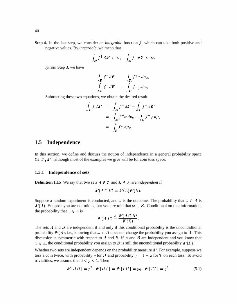
The binomialassetpricing modelprovidesa powerful tool to understandarbitragepricing theoryandprobabilitytheory. In thiscourse,weshalluseit for boththesepurposes.
In thebinomialassetpricing model,we modelstockpricesin discretetime,assumingthatat eachstep,thestockpricewill changeto oneof two possiblevalues.Let usbegin with aninitial positivestockprice +-, . Therearetwo positivenumbers, and . , with
$/01.2) (1.1)
suchthatat thenext period,thestockpricewill beeither 3+4, or .5+-, . Typically, we take and .to satisfy $676897. , so changeof the stockprice from +-, to :+-, representsa downwardmovement,andchangeof the stockprice from + , to .;+ , representsan upward movement. It iscommonto alsohave < = , andthis will be thecasein many of our examples.However, strictlyspeaking,for whatwe areaboutto doweneedto assumeonly (1.1)and(1.2)below.
Of course,stockpricemovementsaremuchmorecomplicatedthanindicatedby thebinomialassetpricing model.We considerthis simplemodelfor threereasons.First of all, within this modeltheconceptof arbitragepricingandits relationto risk-neutralpricing is clearlyilluminated.Secondly,themodelis usedin practicebecausewith a sufficientnumberof steps,it providesa good,compu-tationally tractableapproximationto continuous-timemodels.Thirdly, within thebinomialmodelwe candevelop the theoryof conditionalexpectationsandmartingaleswhich lies at the heartofcontinuous-timemodels.
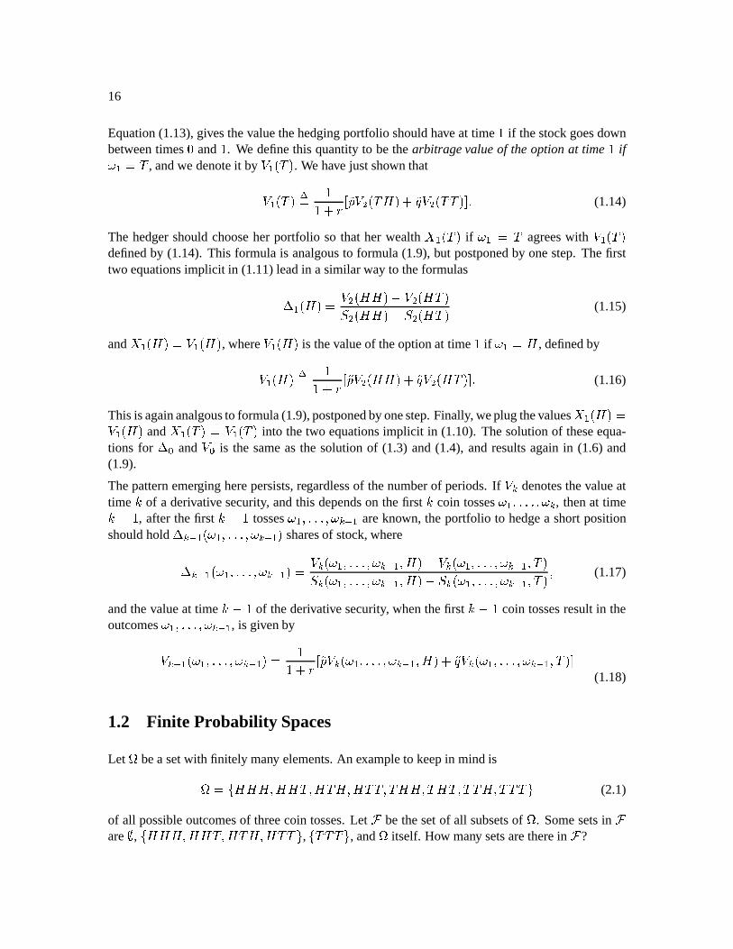
With this third motivation in mind, we develop notationfor the binomial model which is a bitdifferentfrom thatnormallyfoundin practice.Let usimaginethatwe aretossinga coin,andwhenwe geta “Head,” thestockpricemovesup, but whenwe get a “Tail,” thepricemovesdown. Wedenotethepriceat time by +">#?@".5+-, if thetossresultsin head(H), andby +">A(":+-, if it
11
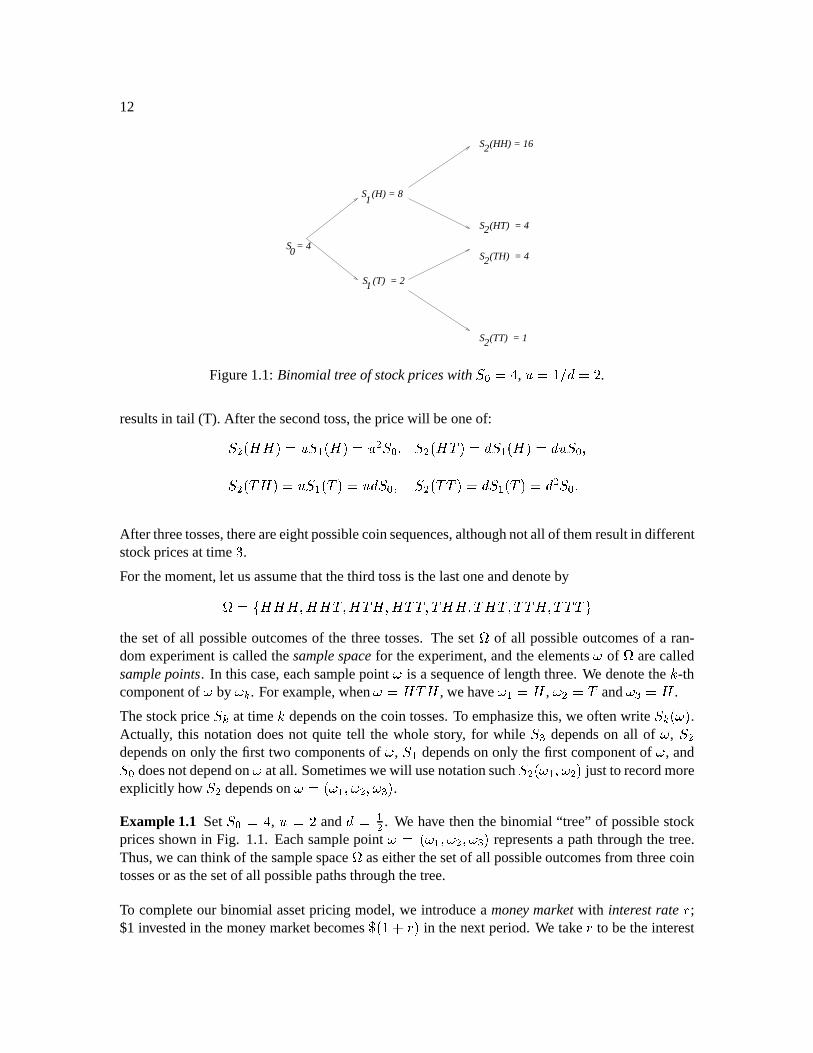
12
S = 40
S (H) = 8
S (T) = 2
S (HH) = 16
S (TT) = 1
S (HT) = 4
S (TH) = 4
1
1
2
2
2
2
Figure1.1: Binomialtreeof stock priceswith +-,(CB , .ED%F .resultsin tail (T). After thesecondtoss,thepricewill beoneof:+2G%#?@?@H.;+"I#?@J. G +-,K)L+2G%#?MA("3+NO#?@J:.5+4,>)+2G%A(?@".5+">A(J.5:+-,K) +2G%APA(JQ3+"IA(JQ G +-,%RAfter threetosses,thereareeightpossiblecoinsequences,althoughnotall of themresultin differentstockpricesat time S .For themoment,let usassumethatthethird tossis thelastoneanddenotebyT VUK?W?@?M)*?@?MAP)?MAX?M)*?YAPA()AP?@?M)A(?MAP)APA(?M)APAPA[Zthe setof all possibleoutcomesof the threetosses.The set
Tof all possibleoutcomesof a ran-
domexperimentis calledthesamplespacefor theexperiment,andtheelements\ ofT
arecalledsamplepoints. In this case,eachsamplepoint \ is a sequenceof lengththree.We denotethe ] -thcomponentof \ by \J^ . For example,when\_?MA(? , wehave \`a? , \NGPbA and \Hc(? .
Thestockprice + ^ at time ] dependson thecoin tosses.To emphasizethis,we oftenwrite + ^ d\a .Actually, this notationdoesnot quite tell the whole story, for while +-c dependson all of \ , +2Gdependson only thefirst two componentsof \ , +N dependson only thefirst componentof \ , and+ , doesnotdependon \ atall. Sometimeswewill usenotationsuch+ G d\ )e\ G just to recordmoreexplicitly how +fG dependson \_gd\hi)e\NGI)e\HcI .Example1.1 Set + , gB , .9LF and j G . We have thenthebinomial “tree” of possiblestockpricesshown in Fig. 1.1. Eachsamplepoint \Qkd\`l)\NGK)e\Hci representsa paththroughthe tree.Thus,we canthink of thesamplespace
Taseitherthesetof all possibleoutcomesfrom threecoin
tossesor asthesetof all possiblepathsthroughthetree.
To completeour binomialassetpricing model,we introducea money marketwith interestrate ;$1 investedin themoney marketbecomesm5hn0K in thenext period.We take to betheinterest
CHAPTER1. Introductionto ProbabilityTheory 13
ratefor bothborrowingandlending. (This is not asridiculousasit first seems,becausein a manyapplicationsof themodel,anagentis eitherborrowing or lending(not both)andknowsin advancewhich shewill bedoing; in suchanapplication,sheshouldtake to betherateof interestfor heractivity.) We assumethat o`n0p0.fR (1.2)
Themodelwouldnotmakesenseif wedid nothave thiscondition.For example,if "nqpr0. , thentherateof returnon themoney marketis alwaysat leastasgreatasandsometimesgreaterthanthereturnon thestock,andnoonewould investin thestock.Theinequality <r`n1 cannothappenunlesseither is negative(whichneverhappens,exceptmaybeonceuponatimein Switzerland)or9rL . In the lattercase,thestockdoesnot really go “down” if we geta tail; it just goesup lessthanif we hadgottena head.Oneshouldborrow money at interestrate andinvestin the stock,sinceevenin theworstcase,thestockpricerisesat leastasfastasthedebtusedto buy it.
With the stock as the underlyingasset,let us considera Europeancall option with strike priceskt $ andexpirationtime . Thisoptionconferstheright to buy thestockat time fors
dollars,andsois worth +"` s at time if +"` s is positiveandis otherwiseworthzero.We denotebyu Id\aJg#+NOd\a" s wv6xQyzKU>+NOd\a| s )*$:Zthevalue(payoff) of this optionat expiration. Of course,
u O\a actuallydependsonly on \h , andwecananddosometimeswrite
u >\`e ratherthanu Id\a . Ourfirst taskis to computethearbitrage
priceof thisoptionat timezero.
Supposeat time zeroyou sell thecall foru , dollars,where
u , is still to bedetermined.You nowhave anobligationto pay off #.;+-,( s v if \`~L? andto payoff #:+-,( s v if \`~A . Atthe time you sell theoption,you don’t yet know which value \` will take. You hedgeyour shortpositionin theoptionby buying , sharesof stock,where , is still to bedetermined.Youcanusetheproceeds
u , of thesaleof theoption for this purpose,andthenborrow if necessaryat interestrate to completethe purchase.If
u , is morethannecessaryto buy the /, sharesof stock,youinvesttheresidualmoney at interestrate . In eithercase,youwill have
u , , + , dollarsinvestedin themoney market,wherethisquantitymight benegative. Youwill alsoown /, sharesof stock.
If thestockgoesup,thevalueof yourportfolio (excludingtheshortpositionin theoption)is , + ?W-nVJn0KI u , 9 , + , l)andyou needto have
u I#?@ . Thus,you wantto chooseu , and , sothatu I#?@J/,l+">#?@-n`n6KI u ,9/,I+-,llR (1.3)
If thestockgoesdown, thevalueof yourportfolio is/,I+">A(-n`n6KI u ,9/,I+-,ll)andyou needto have
u A( . Thus,youwantto chooseu , and , to alsohaveu IA(J/,l+">A[nVJn0KI u ,`/,l+-,IlR (1.4)
14
Thesearetwo equationsin two unknowns,andwesolve thembelow
Subtracting(1.4)from (1.3),weobtainu #?@H u A(J , #+ #?@H9+ A(l) (1.5)
sothat /,P u I#?@" u OA(+ #?@"q+ A( R (1.6)
This is a discrete-timeversionof thefamous“delta-hedging”formulafor derivativesecurities,ac-cordingto which thenumberof sharesof anunderlyingasseta hedgeshouldhold is thederivative(in the senseof calculus)of the valueof the derivative securitywith respectto the price of theunderlyingasset.This formula is sopervasive thewhena practitionersays“delta”, shemeansthederivative (in thesenseof calculus)just described.Note,however, thatmy definitionof /, is thenumberof sharesof stockoneholdsat time zero,and(1.6) is a consequenceof this definition,notthe definition of , itself. Dependingon how uncertaintyentersthe model, therecan be casesin which thenumberof sharesof stocka hedgeshouldhold is not the(calculus)derivative of thederivativesecuritywith respectto thepriceof theunderlyingasset.
To completethesolutionof (1.3) and(1.4), we substitute(1.6) into either(1.3) or (1.4)andsolveforu , . After somesimplification,this leadsto theformulau ,P `n6 `n0[9.9 u O#?@-n .bJn0K.oq u >A(aR (1.7)
This is thearbitrageprice for theEuropeancall optionwith payoffu at time . To simplify this
formula,wedefine x `n0[9.q ) x .0e`n6K.o9 P ) (1.8)
sothat(1.7)becomes u ,P Jn1H u I#?@-n u OA[R (1.9)
Becausewe have taken 9g. , both
and
aredefined,i.e.,thedenominatorin (1.8) is not zero.Becauseof (1.2),both
and
arein the interval $)II , andbecausethey sumto , we canregardthemasprobabilitiesof ? and A , respectively. They arethe risk-neutral probabilites.They ap-pearedwhenwe solvedthe two equations(1.3) and(1.4), andhave nothingto do with the actualprobabilitiesof getting ? or A on thecoin tosses.In fact,at this point, they arenothingmorethana convenienttool for writing (1.7)as(1.9).
We now considera Europeancall which paysoffs
dollarsat time F . At expiration,thepayoff of
this option isu G x8#+ G s v , where
u G and + G dependon \ and \ G , thefirst andsecondcointosses.Wewantto determinethearbitragepricefor thisoptionat timezero.Supposeanagentsellstheoptionat time zerofor
u , dollars,whereu , is still to bedetermined.Shethenbuys , shares
CHAPTER1. Introductionto ProbabilityTheory 15
of stock,investingu ,P/,l+-, dollarsin themoney marketto financethis. At time , theagenthas
a portfolio (excludingtheshortpositionin theoption)valuedat (x/,I+NHn`n6KI u ,9/,I+-,llR (1.10)
Althoughwe do not indicateit in thenotation,+" andtherefore dependon \` , theoutcomeof
thefirst coin toss.Thus,therearereally two equationsimplicit in (1.10): O#?@x /,i+N>#?@ne`n6KI u ,a9,I+-,iO) IA(x /,i+N>A(-nJn6KI u ,9/,I+-,IlRAfter thefirst coin toss,theagenthas
dollarsandcanreadjustherhedge.Supposeshedecidestonow hold sharesof stock,where is allowedto dependon \ becausetheagentknowswhatvalue \` hastaken.Sheinveststheremainderof herwealth,
`6<+" in themoney market.Inthenext period,herwealthwill begivenby theright-handsideof thefollowing equation,andshewantsit to be
u G . Therefore,shewantsto haveu G<*+2GJnhn6>E J9<*+"lR (1.11)
Althoughwedonot indicateit in thenotation,+2G andu G dependon \` and \NG , theoutcomesof the
first two coin tosses.Consideringall four possibleoutcomes,wecanwrite (1.11)asfour equations:u G #?@?@ ?Ww+ G ?W?@;nJn0KI #?@"9 #?@+ #?@l)u G%?A[ <O?Ww+2G>?A[ne`n6KI i?W"<O?Ww+"O?Wwl)u G%A(?@ <OA(+2GKA(?@-n`n6KI OA[H<IA(+"IA(wl)u GKAPA( <OA(+2GKAPA(-nVJn0KI lA(J9<>A(+"iA(lRWe now havesix equations,thetwo representedby (1.10)andthefour representedby (1.11),in thesix unknowns
u , , /, , O#?@ , <>A( , >#?@ , and >A[ .
To solvetheseequations,andtherebydeterminethearbitragepriceu , at timezeroof theoptionand
thehedgingportfolio , , #?@ and A( , webegin with thelasttwou G>A[?W >A(+2GEA(?@-nJn0KI iA("<OA(+"IA(O)u G>APA( >A(+2GEAPA(2ne`n6KI iA(J9<>A[+"IA(lRSubtractingoneof thesefrom theotherandsolvingfor <OA( , we obtainthe“delta-hedgingfor-mula” <IA(J u G%A(?@" u GKAPA[+fG%A(?@"9+2G%APA( ) (1.12)
andsubstituting this into eitherequation,wecansolvefor A(" `n0 u G A(?@-n u G AA(R (1.13)
16
Equation(1.13),givesthevaluethehedgingportfolio shouldhave at time if thestockgoesdownbetweentimes $ and . We definethis quantityto bethearbitragevalueof theoptionat time if\`aCA , andwe denoteit by
u OA[ . We have justshown thatu OA[Px `n6" u G%A(?@5n u GKAPA(R (1.14)
The hedgershouldchooseher portfolio so that her wealth A( if \ A agreeswith
u A(definedby (1.14). This formula is analgousto formula(1.9),but postponedby onestep.Thefirsttwo equationsimplicit in (1.11)leadin a similarway to theformulas<>?W" u G%?W?@f u G>?A[+2G%?W?@fq+2GK#?MA( (1.15)
and I#?@J u O#?@ , where
u O?W is thevalueof theoptionat time if \`aQ? , definedbyu I#?@x `n0f u GK#?@?W-n u G>?A[R (1.16)
Thisisagainanalgousto formula(1.9),postponedbyonestep.Finally, weplugthevalues #?@Ju O?W and
IA(P u OA[ into thetwo equationsimplicit in (1.10). Thesolutionof theseequa-tions for /, and
u , is the sameasthe solutionof (1.3) and(1.4), andresultsagainin (1.6) and(1.9).
Thepatternemerging herepersists,regardlessof thenumberof periods.Ifu ^ denotesthevalueat
time ] of a derivative security, andthis dependson thefirst ] coin tosses\`I)ERIRER)\N^ , thenat time]<b , after thefirst ]< tosses\hI)IRIRER)\J^l- areknown, the portfolio to hedgea shortpositionshouldhold ^O- d\ )IRERIR)e\ ^O sharesof stock,where ^O- d\ )ERIRIRw)\ ^O- J u ^%\`I)IRERIR)e\N^l-I)?Wf u ^3\`i)ERIRER)\N^O-I)A(+2^3\`I)IRERIR)e\N^l-I)?Wfq+2^:d\`I)ERIRIR)e\N^l-I)wA( ) (1.17)
andthevalueat time ]ob of thederivative security, whenthefirst ]b coin tossesresultin theoutcomes\hI)IRIRER)\N^O- , is givenbyu ^l->d\`l)IRERIR)e\N^O*J `n6"
u ^3d\hi)ERIRIRw)\N^O-I)*?@5n u ^:d\`l)IRIRER)\J^l-I)A[(1.18)
1.2 Finite Probability Spaces
LetT
bea setwith finitely many elements.An exampleto keepin mindisT VUK?W?@?M)*?@?MAP)?MAX?M)*?YAPA()AP?@?M)A(?MAP)APA(?M)APAPA[Z (2.1)
of all possibleoutcomesof threecoin tosses.Let bethesetof all subsetsofT
. Somesetsin are , U>?@?@?)?W?MAP)?jA(?M)?MAaAZ , UIAPAPAZ , and
Titself. How many setsaretherein ?
CHAPTER1. Introductionto ProbabilityTheory 17
Definition 1.1 A probability measure is a function mapping into $)E with the followingproperties:
(i) T J ,(ii) If I)*[GI)ERIRIR is asequenceof disjoint setsin , then gY^* f [^l¡b¢^ 2 #[^KlRProbabilitymeasureshave the following interpretation.Let bea subsetof . Imaginethat
Tis
thesetof all possibleoutcomesof somerandomexperiment.Thereis acertainprobability, between$ and , that whenthat experimentis performed,the outcomewill lie in the set . We think of #[ asthisprobability.
Example1.2 Supposea coin hasprobability c for ? and Gc for A . For the individualelementsofTin (2.1),define pU>?@?@?£Z(¤ cK¥ c ) pU>?@?MAZ(¤ cK¥ G ¤ Gc%¥ ) pU>?MA(?£Z(¤ c¦¥ G ¤ Gc%¥ ) pU>?MAPAZ(§¤ c%¥ ¤ Gc>¥ G ) pUIA[?W?£Z(¤ c¦¥ G ¤ c%¥ ) pUIA(?MAZ(§¤ c%¥ ¤ Gc>¥ G ) pUIAA(?£Z~¤ c ¥ ¤ Gc ¥ G ) pUIAPAAZ~¤ Gc ¥ c R
For ¨< , we define #[` ¢©«ª>¬ pUl\PZ3R (2.2)
For example, pU>?@?@?)?@?A[)?jA(?M)?MAAZa8 S-® c n1F S;® G FS-® n7 S-® FS;® G S )which is anotherwayof sayingthattheprobabilityof ? on thefirst tossis c .As in theaboveexample,it is generallythecasethatwespecifyaprobabilitymeasureononly someof thesubsetsof
Tandthenuseproperty(ii) of Definition1.1to determine #[ for theremaining
setsV¨j . In theaboveexample,wespecifiedtheprobabilitymeasureonly for thesetscontainingasingleelement,andthenusedDefinition1.1(ii) in theform (2.2)(seeProblem1.4(ii)) to determine for all theothersetsin .
Definition 1.2 LetT
be a nonemptyset. A -algebrais a collection ¯ of subsetsofT
with thefollowing threeproperties:
(i) /¨M¯ ,
18
(ii) If V¨¯ , thenits complement(°¨M¯ ,
(iii) If i)(GE)*cK)IRIRER is a sequenceof setsin ¯ , then ± ^ 2 (^ is alsoin ¯ .
Herearesomeimportant -algebrasof subsetsof thesetT
in Example1.2: , ²J«) T³ )´ ²J«) T )OU>?@?W?M)?@?jAP)?jA(?M)?MAaAZ3)UIA(?M?)wAX?MAP)APA[?)APAAZ ³ )(Gµ ²J«) T )OU>?@?W?M)?@?jAZ:)U>?jA(?M)?MAAZ3)UIA(?M?)wAP?A[Z3)OUlAPA(?M)APAPAZ3)andall setswhich canbebuilt by takingunionsof these
³ )Pc¶ g Thesetof all subsetsofT R
To simplify notationa bit, let usdefineP·xVU>?@?@?)?W?MAP)?MAP?)?jAPAZ|¸U>? on thefirst tossZ:)P¹qxVUEA(?@?)wA(?MA()APAP?M)AAPAZa¸UIA on thefirst tossZ3)sothat `VU>) T )*·()P¹"Z3)andlet usdefine ··¸xVU>?@?@?M)*?@?jAZVU>?@? on thefirst two tossesZ3) ·¹ xVU>?MA(?M)*?MAPAZ`VU>?MA on thefirst two tossesZ3) ¹5· xVUIA(?@?M)A(?MAZ`VUIA[? on thefirst two tossesZ3) ¹5¹ xVUEAPA(?M)APAPAZaVUIAPA on thefirst two tossesZ3)sothat (Gº U>) T )*·a·[)*·¹H)*¹5·)P¹;¹N) · )* ¹ )* ·a· ±M ¹;· )* ·· ±M ¹;¹ )* ·a¹ ± ¹5· ) ·¹ ± ¹5¹ ) °·· ) °·¹ )* °¹5· )* °¹5¹ Z3RWe interpret -algebrasasarecordof information.Supposethecoin is tossedthreetimes,andyouarenot told theoutcome,but you aretold, for every setin whetheror not theoutcomeis in thatset.For example,you would betold thattheoutcomeis not in andis in
T. Moreover, you might
betold that theoutcomeis not in · but is in ¹ . In effect, you have beentold that thefirst tosswasa A , andnothingmore.The -algebra is saidto containthe“information of thefirst toss”,which is usuallycalledthe“information up to time ”. Similarly, [G containsthe“information of
CHAPTER1. Introductionto ProbabilityTheory 19
thefirst two tosses,” which is the“informationup to time F .” The -algebraPc(Q contains“fullinformation”abouttheoutcomeof all threetosses.Theso-called“tri vial” -algebra , containsnoinformation.Knowing whethertheoutcome\ of thethreetossesis in (it is not)andwhetherit isinT
(it is) tellsyounothingabout\Definition 1.3 Let
Tbeanonemptyfiniteset.A filtrationisasequenceof -algebrasP,%)*)(GE)IRERIR)wP»
suchthateach -algebrain thesequencecontainsall thesetscontainedby theprevious -algebra.
Definition 1.4 LetT
be a nonemptyfinite setandlet be the -algebraof all subsetsofT
. Arandomvariableis a functionmapping
Tinto ¼ .
Example1.3 LetT
begivenby (2.1)andconsiderthebinomialassetpricing Example1.1,where+-,9B , .VF and b G . Then +-, , +" , +2G and +4c areall randomvariables. For example,+2G%#?@?MA(JV. G +-,[LI½ . The“randomvariable” +-, is really not random,since +-,¾\a`VB for all\¿¨ T . Nonetheless,it is a functionmappingT
into ¼ , andthustechnicallya randomvariable,albeita degenerateone.
A randomvariablemapsT
into ¼ , andwe canlook at thepreimageundertherandomvariableofsetsin ¼ . Consider, for example,therandomvariable+2G of Example1.1. Wehave+2GK#?@?@?W"+2GK#?@?MA("I½)+2GK#?MA(?@HQ+2G%#?MAPA("+2G%A[?W?@2Q+2G%A(?MA("bB5)+2GKAPA(?@J+fG>AAPA(J%RLet usconsidertheinterval B5)F%ÀE . Thepreimageunder +2G of this interval is definedto beUO\¨ TÁ +2GKd\a¨ B5)*F%À>ÂZaVUl\0¨ TÁ B/Ã0+2G[Ã0F%À:Z(Q °¹;¹ RThecompletelist of subsetsof
Twe cangetaspreimagesof setsin ¼ is:) T )P··[)*·a¹±j¹5·)P¹;¹H)
andsetswhich canbebuilt by takingunionsof these.This collectionof setsis a -algebra,calledthe -algebra generatedby the randomvariable +2G , andis denotedby `+2G* . The informationcontentof this -algebrais exactly the information learnedby observing+2G . More specifically,supposethecoin is tossedthreetimesandyou do not know theoutcome\ , but someoneis willingto tell you, for eachsetin h#+2G , whether\ is in theset.Youmight betold, for example,that \ isnot in ·· , is in ·¹ ±j ¹5· , andis not in ¹;¹ . Thenyou know thatin thefirst two tosses,therewasa headanda tail, andyou know nothingmore. This informationis thesameyou would havegottenby beingtold thatthevalueof +fG>d\a is B .Note that (G definedearliercontainsall the setswhich arein `#+2G , andevenmore. This meansthattheinformationin thefirst two tossesis greaterthantheinformationin + G . In particular, if youseethefirst two tosses,you candistinguishP·¹ from ¹5· , but you cannotmakethis distinctionfrom knowing thevalueof +2G alone.
20
Definition 1.5 LetT
bea nonemtpyfinite setandlet bethe -algebraof all subsetsofT
. Let
bearandomvariableon T )w . The -algebra h generatedby
is definedto bethecollectionof all setsof theform Ul\b¨ TÁ d\aJ¨@Z , where is a subsetof ¼ . Let ¯ bea sub- -algebraof . Wesaythat
is ¯ -measurableif every setin ` is alsoin ¯ .
Note:We normallywrite simply U ¨Z ratherthan UO\¨ TÁ d\aJ¨MZ .Definition 1.6 Let
Tbea nonempty, finite set,let bethe -algebraof all subsetsof
T, let be
a probabiltymeasureon T )w , andlet
bea randomvariableonT
. Givenany set gÄV ¼ , wedefinethe inducedmeasureof to beÅhÆ ( x pU ¨Z3RIn otherwords,theinducedmeasureof a set tells ustheprobabilitythat
takesa valuein . In
thecaseof +2G abovewith theprobabilitymeasureof Example1.2,somesetsin ¼ andtheir inducedmeasuresare: ÅaÇlÈ %J #¦J$)Å ÇlÈ ¼J T `%)Å ÇlÈ $)*É6" T `%)Å ÇlÈ $)*SE5 pUK+2GKZ~b P¹;¹HJ8 FS ® G RIn fact,theinducedmeasureof + G placesamassof size ¤ c¦¥ G Ê at thenumber I½ , amassof sizeËÊ at the numberB , anda massof size ¤ Gc%¥ G ËÊ at the number . A commonway to recordthis
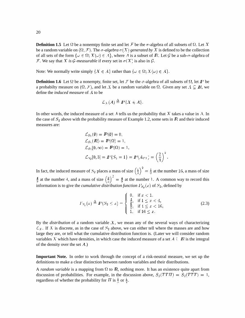
informationis to give thecumulativedistribution function Ì ÇlÈ #Í; of +2G , definedby
Ì ÇlÈ Í5Px +2GÃ0Í;JÎÏÏÏÐ ÏÏÏÑ$) if ÍM%)ËÊ ) if Ã1Íj6B5)ÒÊ ) if BÃ1ÍjI½)%) if I½/Ã0ÍfR (2.3)
By the distribution of a randomvariable
, we meanany of the several waysof characterizingÅ`Æ
. If
is discrete,asin thecaseof +fG above, we caneithertell wherethemassesareandhowlargethey are,or tell whatthecumulative distribution functionis. (Laterwe will considerrandomvariables
whichhavedensities,in whichcasetheinducedmeasureof aset QÄ0 ¼ is theintegral
of thedensityover theset .)
Important Note. In orderto work throughthe conceptof a risk-neutralmeasure,we setup thedefinitionsto makea cleardistinctionbetweenrandomvariablesandtheir distributions.
A randomvariable is a mappingfromT
to ¼ , nothingmore. It hasanexistencequiteapartfromdiscussionof probabilities. For example,in the discussionabove, +2G%APA(?@k+2G>APAPA(/ ,regardlessof whethertheprobabilityfor ? is c or G .
CHAPTER1. Introductionto ProbabilityTheory 21
Thedistributionof a randomvariableis a measure
Å`Æon ¼ , i.e.,a way of assigningprobabilities
to setsin ¼ . It dependsontherandomvariable
andtheprobabilitymeasure weuseinT
. If wesettheprobabilityof ? to be c , then
Å ÇlÈassignsmassÊ to thenumberI½ . If wesettheprobability
of ? to be G , then
Å ÇlÈassignsmass Ë to thenumber I½ . Thedistributionof +2G haschanged,but
therandomvariablehasnot. It is still definedby+2GK#?@?@?W"+2GK#?@?MA("I½)+2GK#?MA(?@HQ+2G%#?MAPA("+2G%A[?W?@2Q+2G%A(?MA("bB5)+2GKAPA(?@J+fG>AAPA(J%RThus,arandomvariablecanhavemorethanonedistribution(a“market”or “objective” distribution,anda “risk-neutral”distribution).
In a similar vein, two different randomvariablescanhave the samedistribution. Supposein thebinomial modelof Example1.1, the probability of ? andthe probability of A is G . ConsideraEuropeancall with strikeprice lB expiring at time F . Thepayoff of thecall at time F is therandomvariable #+ G 0lB: v , which takesthevalue F if \£Q?W?@? or \_?@?MA , andtakesthevalue $ ineveryothercase.Theprobabilitythepayoff is F is Ë , andtheprobabilityit is zerois cË . Consideralsoa Europeanput with strikeprice S expiring at time F . Thepayoff of theput at time F is #S+2G* v ,which takesthevalue F if \gAA(? or \gAAPA . Like thepayoff of thecall, thepayoff of theput is F with probability Ë and $ with probability cË . Thepayoffs of thecall andtheputaredifferentrandomvariableshaving thesamedistribution.
Definition 1.7 LetT
bea nonempty, finite set,let bethe -algebraof all subsetsofT
, let bea probabiltymeasureon T )w , andlet
bea randomvariableon
T. Theexpectedvalueof
is
definedto be Ó x ¢©ª>Ô \a pUl\PZ3R (2.4)
Noticethattheexpectedvaluein (2.4)is definedto beasumoverthesamplespaceT
. SinceT
is afinite set,
cantakeonly finitely many values,whichwelabel Í-l)IRERIR)Í» . We canpartition
Tinto
thesubsetsU JÍ-lZ:)IRIRER)lU »~QÍ»;Z , andthenrewrite (2.4)as Ó x ¢©ª>Ô d\a pUl\PZ »¢^* f ¢©«ª¾Õ ÆJÖ ;× ÖØ d\a pUO\PZ »¢^* f Í;^ ¢©ª%Õ ÆJÖ ;× ÖØ pUl\PZ »¢^* f Í ^ pU ^ QÍ ^ Z »¢^* f Í;^ ÅhÆ U>Í;^KZ3R
22
Thus,althoughtheexpectedvalueis definedasasumover thesamplespaceT
, wecanalsowrite itasa sumover ¼ .
To maketheabove setof equationsabsolutelyclear, we consider+2G with thedistributiongivenby(2.3). Thedefinitionof Ó/+2G is Ó/+2GÙ +2G%?W?@?@ pUK?W?@?£ZHn6+2G%#?@?MA( pU>?@?AZn+2G%#?MA(?@ pU>?MA(?£ZHn1+2G>?AA( pU>?MAPAZn+ G A(?@?@ pUIA[?W?£ZHn1+ G A(?MA( pUIA[?AZn+2G%APA(?@ pUIAPA(?£ZNn6+fG%APAPA(w pUIAPAPAZ I½ÚI #··(2n6BÚI #P·¹±j¹5·-nPÚl P¹;¹H I½ÚI pU>+2GE½:ZanBÚI pU>+2GbBZanbÚI pU>+2GKZ I½Ú ÅaÇOÈ U3I½:Z`nBÚ ÅÇlÈ UIB«Z|nQÚ ÅaÇOÈ U3KZ I½Ú Û n6BÚ BÛ nB~Ú BÛ B3ÜÛ RDefinition 1.8 Let
Tbeanonempty, finite set,let bethe -algebraof all subsetsof
T, let bea
probabiltymeasureon T )< , andlet
bea randomvariableonT
. Thevarianceof
is definedto betheexpectedvalueof 9 Ó G , i.e.,
Var Px ¢©ªKÔ d\a2 Ó G pUl\PZ3R (2.5)
Oneagain,we canrewrite (2.5)asa sumover ¼ ratherthanoverT
. Indeed,if
takesthevaluesÍ )ERIRER)*Í » , then
Var " »¢^* f #Í5^9 Ó G pU QÍ5^KZ »¢^ 2 #Í5^9 Ó G ÅhÆ #Í;^IlR1.3 LebesgueMeasureand the LebesgueIntegral
In thissection,we considerthesetof realnumbers ¼ , which is uncountablyinfinite. We definetheLebesguemeasureof intervalsin ¼ to betheir length.Thisdefinitionandthepropertiesof measuredeterminethe Lebesguemeasureof many, but not all, subsetsof ¼ . The collectionof subsetsof ¼ we consider, andfor which Lebesguemeasureis defined,is thecollectionof Borel setsdefinedbelow.
We useLebesguemeasureto constructthe Lebesgueintegral, a generalizationof the Riemannintegral. We needthis integral because,unlike theRiemannintegral, it canbedefinedon abstractspaces,suchas the spaceof infinite sequencesof coin tossesor the spaceof pathsof Brownianmotion. This sectionconcernsthe Lebesgueintegral on the space ¼ only; the generalizationtootherspaceswill begivenlater.
CHAPTER1. Introductionto ProbabilityTheory 23
Definition 1.9 TheBorel -algebra, denotedÝ# ¼ , is thesmallest -algebracontainingall openintervalsin ¼ . Thesetsin Ý# ¼ arecalledBorel sets.
Everysetwhichcanbewrittendown andjustabouteverysetimaginableis in Ý# ¼ . Thefollowingdiscussionof this factusesthe -algebrapropertiesdevelopedin Problem1.3.
By definition,everyopeninterval #Þ;)*ßl is in Ý~ ¼ , whereÞ and ß arerealnumbers.SinceÝ~# ¼ isa -algebra,every unionof openintervalsis alsoin Ý# ¼ . For example,for every realnumberÞ ,theopenhalf-line Þ5)É6H »K f #Þ;)*Þn6àis aBorel set,asis PÉb)*Þ:J »K 2 #Þ9à")Þ3lRFor realnumbersÞ and ß , theunion PÉb)*Þ:2±9#ßK)É6is Borel. SinceÝ~ ¼ is a -algebra,every complementof a Borelsetis Borel,so Ý# ¼ contains Þ;)*ßw§¤>PÉb)*Þ:2±9#ßK)É6 ¥ ° RThisshowsthateveryclosedinterval is Borel. In addition,theclosedhalf-lines
Þ;)*É6J »> f Þ;)*ÞPn1à«and ePÉb)*Þ¾ »> f Þp9à")*Þ¾areBorel. Half-openandhalf-closedintervalsarealsoBorel,sincethey canbewritten asintersec-tionsof openhalf-linesandclosedhalf-lines.For example,#Þ;)*ßw5gPÉb)ßw3á9#Þ5)É6lREverysetwhich containsonly onerealnumberis Borel. Indeed,if Þ is a realnumber, thenU>Þ«Z( â»> f 3Þp à )*ÞPn à ® RThis meansthatevery setcontainingfinitely many realnumbersis Borel; if ãU>Þ )Þ G )IRERIR)Þ » Z ,then 0 »^ f U>Þ:^KZ:R
24
In fact,everysetcontainingcountablyinfinitely many numbersis Borel; if bVU>Þ«i)Þ3GE)IRERIRZ , then0 »^ f U>Þ:^KZ:RThis meansthat the set of rational numbersis Borel, as is its complement,the setof irrationalnumbers.
Thereare,however, setswhich arenot Borel. We have just seenthatany non-Borelsetmusthaveuncountablymany points.
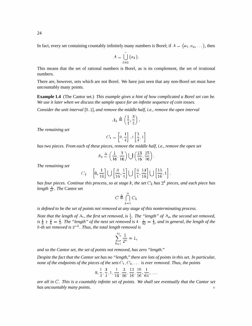
Example1.4 (TheCantorset.) Thisexamplegivesa hint of howcomplicateda Borel setcanbe.Weuseit later whenwediscussthesamplespacefor an infinitesequenceof coin tosses.
Considertheunit interval $)E , andremovethemiddlehalf, i.e., removetheopenintervalxä B ) SB2® RTheremainingset å ` $) B ± SB )E hastwo pieces.Fromeach of thesepieces,removethemiddlehalf, i.e., removetheopenset[Gx I½ ) SI½ ® ISI½ ) IæI½ ® RTheremainingset å G $) I½ SI½ ) B SB ) ISI½ IæI½ )EaRhasfour pieces.Continuethis process,soat stage] , theset
å ^ has F ^ pieces,andeach piecehaslength Ë Ö . TheCantorset å x â^ 2 å ^is definedto bethesetof pointsnot removedat anystageof thisnonterminatingprocess.
Notethat thelengthof , thefirst setremoved,isG . The“length” of (G , thesecondsetremoved,
is Ò n Ò Ë . The“length” of thenext setremovedis BÚ cG Ò , andin general, thelengthof the] -th setremovedis F «^ . Thus,thetotal lengthremovedis¢^* f F ^ ¦)andsotheCantorset,thesetof pointsnot removed,haszero “length.”
Despitethefact that theCantorsethasno“length,” thereare lotsof pointsin thisset.In particular,noneof theendpointsof thepiecesof thesets
å ) å G )ERIRIR is ever removed.Thus,thepoints$) B ) SB )E%) E½ ) SI½ ) ISI½ ) IæI½ ) ½KB )IRIRERare all in
å. This is a countablyinfinite setof points. We shall seeeventuallythat theCantorset
hasuncountablymanypoints. ç
CHAPTER1. Introductionto ProbabilityTheory 25
Definition 1.10 Let Ý~# ¼ bethe -algebraof Borel subsetsof ¼ . A measure on # ¼/)wÝ~# ¼ is afunction è mappingÝ into $)É£ with thefollowing properties:
(i) è`#¦J$ ,(ii) If I)*[GI)ERIRIR is asequenceof disjoint setsin Ý~# ¼ , thenè ^* f [^ ¡ ¢^ 2 è`#(^ElRLebesguemeasure is definedto bethemeasureon # ¼/)wÝ~# ¼ which assignsthemeasureof eachinterval to beits length.Following Williams’sbook,wedenoteLebesguemeasureby è , .A measurehasall thepropertiesof aprobabilitymeasuregivenin Problem1.4,exceptthatthetotalmeasureof thespaceis notnecessarily (in fact, è-,3# ¼JÉ ), oneno longerhastheequationè`# ° JP@è`#[in Problem1.4(iii), andproperty(v) in Problem1.4needsto bemodifiedto say:
(v) If I)(GE)IRERIR is a sequenceof setsin Ý~# ¼ with [é0(G[éÚEÚIÚ and è`#*0É , thenè â^* f [^ ¡ ºêìëíy»>î è|P»lRTo seethattheadditionalrequirmentè`#*0É is neededin (v), considera ¦)*É6l)(GJ F)*É6l)Pc` S)*É6O)IRIRERRThen á ^ 2 [^ , so è-,3#á ^ 2 [^KJ$ , but êìëíyo»>î è,3P»3JQÉ .
WespecifythattheLebesguemeasureof eachinterval is its length,andthatdeterminestheLebesguemeasureof all otherBorel sets.For example,theLebesguemeasureof theCantorsetin Example1.4mustbezero,becauseof the“length” computationgivenat theendof thatexample.
TheLebesguemeasureof asetcontainingonly onepointmustbezero.In fact,sinceU>Þ«ZïÄ Þp à )*Þn à ®for every positiveinteger à , we musthave$/Ã6è-,KU>Þ«ZÃ6è-, Þ/ à )*Þ[n à ® Fà RLetting àjðÉ , weobtain è,KUKÞZ($«R
26
The Lebesguemeasureof a setcontainingcountablymany pointsmustalsobe zero. Indeed,ifbVU>Þ )Þ G )IRERIRZ , then è-,3#[J ¢^ f è-,KU>Þ:^KZ~¢^ f $Q$RTheLebesguemeasureof asetcontaininguncountablymany pointscanbeeitherzero,positiveandfinite, or infinite. We maynot computetheLebesguemeasureof anuncountablesetby addingupthe Lebesguemeasureof its individual members,becausethereis no way to addup uncountablymany numbers.Theintegralwasinventedto getaroundthis problem.
In orderto think aboutLebesgueintegrals,wemustfirst considerthefunctionsto beintegrated.
Definition 1.11 Let ñ be a function from ¼ to ¼ . We saythat ñ is Borel-measurable if the setU>Í£¨q ¼ Á ñNÍ5¨Z is in Ý# ¼ whenever L¨9Ý# ¼ . In thelanguageof Section2, we wantthe -algebra generatedby ñ to becontainedin Ý~ ¼ .Definition 3.4 is purely technicalandhasnothingto do with keepingtrack of information. It isdifficult to conceive of a functionwhich is not Borel-measurable,andwe shallpretendsuchfunc-tions don’t exist. Hencefore,“function mapping ¼ to ¼ ” will mean“Borel-measurablefunctionmapping ¼ to ¼ ” and“subsetof ¼ ” will mean“Borel subsetof ¼ ”.
Definition 1.12 An indicator function ò from ¼ to ¼ is a functionwhich takesonly thevalues$and . We call xVU>ÍY¨ ¼ Á òH#Í;H¾Zthesetindicatedby ò . We definetheLebesgueintegral of ò to beó:ô õ òX¦è-, xCè,3(lRA simplefunction ö from ¼ to ¼ is a linearcombinationof indicators,i.e.,a functionof theformö"#Í5J »¢^* f÷ ^iò3^3#Í;l)whereeachò3^ is of theform ò3^3#Í;Jg² %) if ÍM¨[^:)$) if ÍD¨[^:)andeach÷ ^ is a realnumber. WedefinetheLebesgueintegral of ö to beó õ ö[%è-,x »¢^ 2÷ ^ ó ô õ ò3^E%è-,( »¢^ f÷ ^Oè,3(^ElRLet ñ be a nonnegative function definedon ¼ , possiblytaking the value É at somepoints. WedefinetheLebesgueintegral of ñ to beó%ô õ ñ%è-,xbø*ùúpû ó%ô õ ö[¦è, Á ö is simpleand öHÍ5Ã0ñJ#Í; for every ͨM ¼üR
CHAPTER1. Introductionto ProbabilityTheory 27
It is possiblethatthis integral is infinite. If it is finite, we saythat ñ is integrable.
Finally, let ñ bea functiondefinedon ¼ , possiblytakingthevalue É atsomepointsandthevaluePÉ atotherpoints.We definethepositiveandnegativepartsof ñ to beñ v #Í;PxyzKUKñNÍ5l)$:Z3)ñ #Í;PxyzK;U3PñJ#Í5O)*$:Z3)respectively, andwedefinetheLebesgueintegral of ñ to beó ô õ ñ(¦è-,ïx ó ô õ ñ v ¦è,0 ó ô õ ñ %è-,K)providedtheright-handsideis notof theform ÉýMÉ . If both þ ô õ ñ v %è-, and þ ô õ ñ %è-, arefinite(or equivalently, þ ô õÿ ñ ÿ ¦è,[0É , since
ÿ ñ ÿ ñ v n6ñ ), wesaythat ñ is integrable.
Let ñ beafunctiondefinedon ¼ , possiblytakingthevalue É atsomepointsandthevalue PÉ atotherpoints.Let bea subsetof ¼ . Wedefineó ¬ ñ[¦è , x ó ô õ ¬ ñ¦è , )where ¬ Í5Pxg² %) if ÍM¨p)$) if ÍD¨p)is the indicator functionof .
TheLebesgueintegral just definedis relatedto theRiemannintegral in onevery importantway: iftheRiemannintegral þ PñJ#Í5:Í is defined,thentheLebesgueintegral þ ñ[¦è, agreeswith theRiemannintegral. TheLebesgueintegralhastwo importantadvantagesover theRiemannintegral.The first is that the Lebesgueintegral is definedfor morefunctions,aswe show in the followingexamples.
Example1.5 Let bethesetof rationalnumbersin $«)I , andconsiderñWx . Beingacountableset, hasLebesguemeasurezero,andsotheLebesgueintegralof ñ over $)I isó , ñ¦è-,XQ$RTo computethe Riemannintegral þ , ñJ#Í5w3Í , we choosepartition points $8Í,M7Í-8ÚEÚIÚJÍ»b anddivide the interval $)E into subintervals Í,K)*Í4Â) Í4*)*Í;G)ERIRER) Í»¦-I)*Í»E . In eachsubinterval Í5^O-I)*Í5^i thereis a rationalpoint ^ , where ñN ^I[ , andthereis alsoan irrationalpoint ^ , where ñJ# ^ h$ . We approximatetheRiemannintegral from above by theuppersum»¢^* f ñJ ^ IÍ ^ qÍ ^l- h »¢^* f aÚ:#Í ^ qÍ ^O- J%)andwealsoapproximateit from below by the lowersum»¢^* f ñJ#E^IIÍ5^P9Í;^l-*h »¢^* f $(Ú:#Í5^qÍ5^O-*J$R
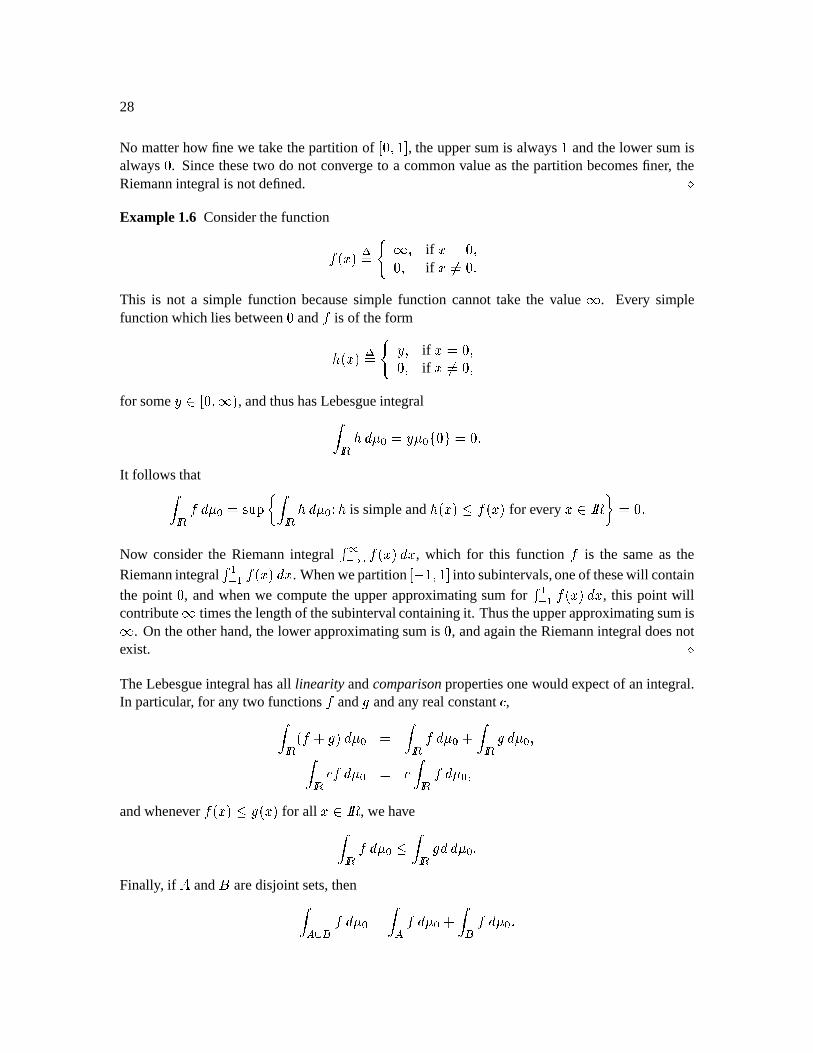
28
No matterhow fine we takethepartitionof $)I , theuppersumis always andthelower sumisalways $ . Sincethesetwo do not converge to a commonvalueasthepartitionbecomesfiner, theRiemannintegral is notdefined. çExample1.6 ConsiderthefunctionñJ#Í5x ² Éb) if ÍQ$)$) if Í Q$RThis is not a simple function becausesimple function cannottake the value É . Every simplefunctionwhich lies between$ and ñ is of theformö"#Í5[xg² ) if Í<$)$) if Í $)for some ¨ $)*É6 , andthushasLebesgueintegraló ô õ ö[%è-,P è-,KU>$:Z($RIt followstható ô õ ñ%è-,Pbø*ùú û ó ô õ ö[%è-, Á ö is simpleand öH#Í;Ã0ñJ#Í5 for every ͨ ¼ ü $«RNow considerthe Riemannintegral þ ñJ#Í;5:Í , which for this function ñ is the sameas the
Riemannintegral þ - ñJ#Í5;3Í . Whenwepartition ¦)I into subintervals,oneof thesewill contain
the point $ , andwhenwe computethe upperapproximatingsumfor þ - ñJ#Í5;3Í , this point willcontribute É timesthelengthof thesubintervalcontainingit. ThustheupperapproximatingsumisÉ . On theotherhand,thelowerapproximatingsumis $ , andagaintheRiemannintegraldoesnotexist. çTheLebesgueintegralhasall linearity andcomparisonpropertiesonewouldexpectof anintegral.In particular, for any two functions ñ and ò andany realconstant÷ ,ó%ô õ #ñ/n£ò55¦è-,µ ó¦ô õ ñ(¦è-,`n ó%ô õ òP%è-,%)ó ô õ ÷ ñ%è , ÷ ó ô õ ñ%è , )andwhenever ñJ#Í;ÃòfÍ5 for all ͨ ¼ , wehaveó%ô õ ñ¦è-,~à ó%ô õ ò5a¦è-,IRFinally, if and aredisjoint sets,thenó ¬ ñ¦è-,X ó ¬ ñ¦è-,`n ó ñ¦è,%R
CHAPTER1. Introductionto ProbabilityTheory 29
Therearethreeconvergencetheoremssatisfiedby the Lebesgueintegral. In eachof thesethe sit-uationis that thereis a sequenceof functions ñ » )*࣠¦)*F)ERIRlR converging pointwiseto a limitingfunction ñ . Pointwiseconvergencejustmeansthatê ëíy»>î ñ » Í5JñJ#Í; for every ͨM ¼/RThereareno suchtheoremsfor the Riemannintegral, becausethe Riemannintegral of the limit-ing function ñ is too oftennot defined. Beforewe statethe theorems,we giventwo examplesofpointwiseconvergencewhicharisein probabilitytheory.
Example1.7 Considera sequenceof normaldensities,eachwith variance andthe à -th havingmeanà : ñE»#Í;Px F ! #"
ÈÈ RTheseconvergepointwiseto thefunctionñJ#Í5J$ for every ÍM¨ ¼/RWe have þ ô õ ñI»:%è-,( for every à , so ê ëíy<»>î þ ô õ ñE»%è-,P , but þ ô õ ñ(¦è-,($ . çExample1.8 Considerasequenceof normaldensities,eachwith mean$ andthe à -th having vari-ance » : ñ » #Í5Px $ àF
ÈÈ RTheseconvergepointwiseto thefunctionñJ#Í5x² Éb) if ÍQ$)$) if Í Q$RWe have again þ ô õ ñE»%è-,@ for every à , so êìëíyo»>î þ ô õ ñE»%è-, , but þ ô õ ñ¦è,@ý$ . Thefunction ñ is nottheDiracdelta;theLebesgueintegralof this functionwasalreadyseenin Example1.6to bezero. çTheorem 3.1 (Fatou’s Lemma)Let ñE»-)*à@%)*F«)IRIRlR bea sequenceof nonnegativefunctionscon-verging pointwiseto a function ñ . Thenó ô õ ñ%è-,Ã6ê ëíy6ë&%'»>î ó ô õ ñE»a¦è,%RIf ê ë yo»>î þ ô õ ñI»%è-, is defined,thenFatou’sLemmahasthesimplerconclusionó%ô õ ñ%è-,Ãêìëíy»>î ó3ô õ ñE»a¦è-,%RThis is thecasein Examples1.7and1.8,whereê ë y»>î ó%ô õ ñE»a¦è-,P%)
30
while þ ô õ ñ¦è-,ï$ . We couldmodify eitherExample1.7 or 1.8 by setting ò¾»jgñE» if à is even,but ò » F%ñ » if à is odd. Now þ ô õ ò » %è , ä if à is even,but þ ô õ ò » ¦è , 7F if à is odd. ThesequenceU>þ ô õ ò%»a¦è-,KZ »> f hastwo clusterpoints, and F . By definition, the smallerone, , isê ëíy6ë&%'i»Kî þ ô õ ò%»a¦è-, andthelargerone, F , is êìëíyø*ùú »>î þ ô õ ò%»a¦è, . Fatou’sLemmaguaranteesthateventhesmallerclusterpointwill begreaterthanor equalto theintegralof thelimiting function.
Thekey assumptionin Fatou’sLemmais thatall thefunctionstakeonlynonnegativevalues.Fatou’sLemmadoesnotassumemuchbut it is is not verysatisfyingbecauseit doesnotconcludetható ô õ ñ%è-,Pºêìëíy»>î ó ô õ ñE»a¦è-,%RTherearetwo setsof assumptionswhich permitthisstrongerconclusion.
Theorem 3.2 (MonotoneConvergenceTheorem)Let ñE»5)*à@ %)*F)ERIRER bea sequenceof functionsconvergingpointwiseto a function ñ . Assumethat$/Ã1ñ%>Í5Ã0ñKG%#Í;Ã0ñEc3#Í5ÃÚEÚIÚ for every Íj¨ ¼/RThen ó%ô õ ñ%è-,Pºêìëíy»>î ó3ô õ ñE»a¦è-,%)where bothsidesareallowedto be É .
Theorem 3.3 (DominatedConvergenceTheorem)Let ñE»5)àã%)*F)ERIRER bea sequenceof functions,which maytakeeitherpositiveor negativevalues,converging pointwiseto a function ñ . Assumethat there is a nonnegativeintegrablefunction ò (i.e., þ ô õ òP%è-,0É ) such thatÿ ñE»#Í5 ÿ ÃòfÍ5 for every ÍM¨ ¼ for every à"RThen ó%ô õ ñ%è-,Pºêìëíy»>î ó3ô õ ñE»a¦è-,%)andbothsideswill befinite.
1.4 GeneralProbability Spaces
Definition 1.13 A probabilityspace T )) consistsof threeobjects:
(i)T
, a nonemptyset, called the samplespace, which containsall possibleoutcomesof somerandomexperiment;
(ii) , a -algebraof subsetsofT
;
(iii) , aprobabilitymeasureon T )< , i.e.,afunctionwhichassignsto eachset ¨j anumber #[¨ $«)I , which representstheprobabilitythat theoutcomeof therandomexperimentlies in theset .
CHAPTER1. Introductionto ProbabilityTheory 31
Remark 1.1 WerecallfromHomeworkProblem1.4thataprobabilitymeasure hasthefollowingproperties:
(a) #%J$ .(b) (Countableadditivity) If )* G )ERIRER is asequenceof disjoint setsin , then gY^* f [^l¡b¢^ 2 #[^KlR(c) (Finiteadditivity) If à is a positiveintegerand I)IRERIR)P» aredisjoint setsin , then # ±£ÚIÚEÚ*±j » J # -nÚIÚEÚ*n6 » lR(d) If and aresetsin and Ä( , then ) (2n1 )+*P[lR
In particular, )r0 #[lR(d) (Continuityfrom below.) If I)*[GI)ERIRER is asequenceof setsin with PÄ0[G(ÄQÚIÚIÚ , then ^* f [^ ¡ ºêìëíy»>î #»5lR(d) (Continuityfrom above.) If )* G )ERIRER is a sequenceof setsin with é0 G éÚIÚEÚ , then g â^* f [^l¡bºêìëíy»>î #»5lRWe have alreadyseensomeexamplesof finite probabilityspaces.We repeattheseandgive someexamplesof infinite probabilityspacesaswell.
Example1.9 Finitecoin tossspace.Tossa coin à times,so that
Tis the setof all sequencesof ? and A which have à components.
We will usethis spacequitea bit, andsogive it a name:T » . Let bethecollectionof all subsets
ofT » . Supposetheprobabilityof ? on eachtossis , a numberbetweenzeroandone. Thenthe
probabilityof A is xãa . For each\£d\`I)\JGI)ERIRIRw)\H»3 inT » , wedefine pUl\PZïx -, =/. )0)13254 ·6 » © Ú 7, =/. )0)18294 ¹6 » © R
For eachV¨j , wedefine #[ x ¢©«ª>¬ pUl\PZ3R (4.1)
Wecandefine #[ thiswaybecause hasonly finitely many elements,andsoonly finitely manytermsappearin thesumontheright-handsideof (4.1). ç
32
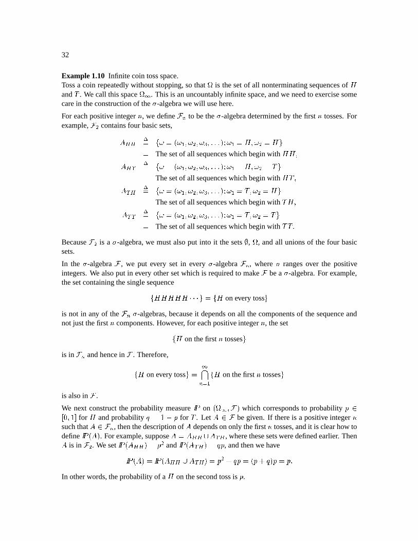
Example1.10 Infinite coin tossspace.Tossa coin repeatedlywithout stopping,sothat
Tis thesetof all nonterminatingsequencesof ?
and A . We call thisspaceT . This is anuncountablyinfinite space,andwe needto exercisesome
carein theconstructionof the -algebrawewill usehere.
For eachpositive integer à , we defineP» to bethe -algebradeterminedby thefirst à tosses.Forexample,[G containsfour basicsets,·a· x Ul\qg\`i)e\NGK)\"c>)ERIRIR Á \`J?M)\NG?£Z Thesetof all sequenceswhich begin with ?W?M)·¹ x Ul\qg\`i)e\NGK)\"c>)ERIRIR Á \`J?M)\NGbAZ Thesetof all sequenceswhich begin with ?A[)¹5· x Ul\qg\`i)e\NGK)\"c>)ERIRIR Á \`JbA()e\NG`Q?9Z Thesetof all sequenceswhich begin with A(?)P¹;¹ x Ul\qg\`i)e\NGK)\"c>)ERIRIR Á \`JbA()e\NG`CAZ Thesetof all sequenceswhich begin with APA(RBecause(G is a -algebra,we mustalsoput into it thesets , T , andall unionsof the four basicsets.
In the -algebra , we put every set in every -algebra » , where à rangesover the positiveintegers.We alsoput in every othersetwhich is requiredto make bea -algebra.For example,thesetcontainingthesinglesequenceUK?W?@?@?@?VÚIÚIÚeZ~VU>? onevery tossZis not in any of the » -algebras,becauseit dependson all thecomponentsof thesequenceandnot just thefirst à components.However, for eachpositiveinteger à , thesetU>? on thefirst à tossesZis in P» andhencein . Therefore,U>? onevery tossZ â»> f UK? onthefirst à tossesZis alsoin .
We next constructthe probability measure on T )< which correspondsto probability ¨ $)E for ? andprobability ( for A . Let L¨9 begiven. If thereis a positive integer àsuchthat Q¨jP» , thenthedescriptionof dependsononly thefirst à tosses,andit is clearhow todefine #[ . For example,supposeb ·· ±/ ¹;· , wherethesesetsweredefinedearlier. Then is in (G . We set #·a·` G and #¹5·J , andthenwehave (h #P··6±¹5·(J G n g n RIn otherwords,theprobabilityof a ? on thesecondtossis .
CHAPTER1. Introductionto ProbabilityTheory 33
Let usnow considera set ¨q for which thereis no positive integer à suchthat L¨ . Suchis thecasefor theset UK? onevery tossZ . To determinetheprobabilityof thesesets,we write themin termsof setswhich arein P» for positive integers à , andthenusethepropertiesof probabilitymeasureslistedin Remark1.1. For example,UK? on thefirst tossZ é U>? on thefirst two tossesZé U>? on thefirst threetossesZé ÚIÚIÚ;)and â»K f U>? on thefirst à tossesZVU>? onevery tossZ3RAccordingto Remark1.1(d)(continuityfrom above), pUK? onevery tossZ(ê ëíy»Kî pUK? on thefirst à tossesZ(ºê ëíy»>î » RIf , then pU>? onevery tossZ( ; otherwise, pU>? onevery tossZ($ .A similarargumentshowsthatif $/ sothat $/ , theneverysetin
T whichcontainsonly oneelement(nonterminatingsequenceof ? and A ) hasprobabilityzero,andhencevery setwhich containscountablymany elementsalsohasprobabiliyzero.We arein a casevery similar toLebesguemeasure:every point hasmeasurezero,but setscanhave positive measure.Of course,theonly setswhich canhave positiveprobabiltyin
T arethosewhich containuncountablymanyelements.
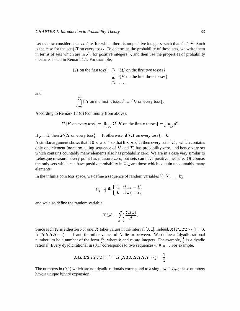
In theinfinite coin tossspace,wedefineasequenceof randomvariables&2I)w&GE)IRIRER by&-^3d\ax² if \ ^ ?)$ if \N^[bA()andwealsodefinetherandomvariable d\a" »¢^ 2 &^:d\aF ^ RSinceeach&-^ is eitherzeroor one,
takesvaluesin theinterval $)Ii . Indeed,
APAPAPA@ÚIÚEÚJ$ , #?@?@?W?QÚIÚEÚ@º and the other valuesof
lie in between. We definea “dyadic rationalnumber”to bea numberof the form
.G Ö , where ] and : areintegers. For example, cË is a dyadicrational.Every dyadicrationalin (0,1)correspondsto two sequences\¨ T . For example, #?@?AAPAPAPAÚEÚIÚJ #?MA(?@?@?W?M?ÚEÚIÚJ SB RThenumbersin (0,1)whicharenotdyadicrationalscorrespondto asingle \0¨ T ; thesenumbershave auniquebinaryexpansion.
34
Wheneverweplacea probabilitymeasure on T ) , wehaveacorrespondinginducedmeasureÅ Æ
on $«)I . For example,if weset G in theconstructionof thisexample,thenwe haveÅhÆ $«) F ïQ pU First tossis AZ( F )ÅhÆ F )I~Q pU First tossis ?9Z( F )ÅhÆ $«) B ïQ pU First two tossesare AAZ( B )ÅhÆ B ) F Q pU First two tossesare A[?9Z( B )Å Æ F ) SB Q pU First two tossesare ?MAZ( B )ÅhÆ SB )I~Q pU First two tossesare ?@?£Z( B RContinuingthisprocess,wecanverify thatfor any positiveintegers] and : satisfying$/à :L0F ^ :F ^ æ)wehave Å`Æ :L1F ^ ) :F ^ F ^ RIn otherwords,the
Å`Æ-measureof all intervalsin $)E whoseendpointsaredyadicrationalsis the
sameastheLebesguemeasureof theseintervals.Theonly waythiscanbeis for
ÅhÆto beLebesgue
measure.
It is interesingto considerwhat
Å Æwould look like if we takea valueof otherthan G whenwe
constructtheprobabilitymeasure onT
.
We concludethis examplewith anotherlook at theCantorsetof Example3.2. LetT<; 6 1>= be the
subsetofT
in which every even-numberedtossis thesameastheodd-numberedtossimmediatelyprecedingit. For example,?W?MAPAAPA(?@? is thebeginningof asequencein
T?; 6 1>= , but ?MA is not.Considernow thesetof realnumberså ! xVU \a Á \q¨ T?; 6 1>= Z3RThe numbersbetween Ë ) G canbewritten as
d\a , but the sequence\ mustbegin with eitherA(? or ?MA . Therefore,noneof thesenumbersis in
å ! . Similarly, thenumbersbetween A@ ) cA@ canbewritten as
d\a , but thesequence\ mustbegin with APAPA[? or APA(?MA , sononeof thesenumbersis in
å ! . Continuingthisprocess,weseethat
å ! will notcontainany of thenumberswhichwereremoved in the constructionof the Cantorset
åin Example3.2. In otherwords,
å ! Ä å .With a bit morework, onecanconvinceonselfthat in fact
å ! å , i.e., by requiringconsecutivecoin tossesto bepaired,we areremoving exactly thosepointsin $«)I which wereremovedin theCantorsetconstructionof Example3.2. ç
CHAPTER1. Introductionto ProbabilityTheory 35
In additionto tossinga coin, anothercommonrandomexperimentis to pick a number, perhapsusinga randomnumbergenerator. Herearesomeprobabilityspaceswhich correspondto differentwaysof pickinga numberat random.
Example1.11Supposewe choosea numberfrom ¼ in sucha way that we are sureto get either , B or I½ .Furthermore,weconstructtheexperimentsothattheprobabilityof getting is
ËÊ , theprobabilityofgetting B is
ËÊ andtheprobabilityof getting I½ is Ê . We describethis randomexperimentby takingTto be ¼ , to be Ý# ¼ , andsettingup theprobabilitymeasuresothat pU3KZ B Û )( pUIB«Z( B Û )P pU3E½:Z~ Û R
This determines #[ for every set ¨@Ý~ ¼ . For example,theprobabilityof theinterval #$)*æ>isÒÊ , becausethis interval containsthenumbers and B , but not thenumberI½ .
Theprobabilitymeasuredescribedin this exampleis
Å ÇOÈ, themeasureinducedby thestockprice+2G , whentheinitial stockprice +4,XCB andtheprobabilityof ? is c . Thisdistributionwasdiscussed
immediatelyfollowing Definition2.8. çExample1.12 Uniform distributionon $)E .Let
T $)I andlet §Ý~ $)Ii , thecollectionof all Borel subsetscontaininedin $)Ii . ForeachBorelset VÄ $«)I ,wedefine (hbè-,#[ tobetheLebesguemeasureof theset.Becauseè , $)E«ã , thisgivesusa probabilitymeasure.
This probabilityspacecorrespondsto therandomexperimentof choosinga numberfrom $)E sothateverynumberis “equallylikely” to bechosen.Sincethereareinfinitely meannumbersin $«)I ,thisrequiresthateverynumberhaveprobabiltyzeroof beingchosen.Nonetheless,wecanspeakoftheprobabilitythat thenumberchosenlies in a particularset,andif thesethasuncountablymanypoints,thenthis probabilitycanbepositive. çI know of no way to designa physicalexperimentwhich correspondsto choosinga numberatrandomfrom $«)I so thateachnumberis equallylikely to bechosen,just asI know of no way totossa coin infinitely many times. Nonetheless,bothExamples1.10and1.12provide probabilityspaceswhichareoftenusefulapproximationsto reality.
Example1.13 Standardnormaldistribution.Definethestandardnormaldensity
P#Í5x FB Í GF RLet
T ¼ , gCÝ~# ¼ andfor everyBorel set VÄ0 ¼ , define ([x ó ¬ o%è-,KR (4.2)
36
If in (4.2)is aninterval Þ;)*ßw , thenwecanwrite (4.2)asthelessmysteriousRiemannintegral:
Þ;)*ßwNx ó F Í GF 3ÍfRThiscorrespondsto choosingapointat randomontherealline,andeverysinglepointhasprobabil-ity zeroof beingchosen,but if a set is given,thentheprobabilitythepoint is in thatsetis givenby (4.2). çThe constructionof the integral in a generalprobabilityspacefollows the samestepsasthe con-structionof Lebesgueintegral. We repeatthisconstructionbelow.
Definition 1.14 Let T )) beaprobabilityspace,andlet
bearandomvariableonthisspace,i.e.,a mappingfrom
Tto ¼ , possiblyalsotakingthevaluesCÉ .D If
is an indicator, i.e, d\a" ¬ d\aJ ² if \ ¨M)$ if \ ¨M(°)
for someset V¨j , wedefine ó Ô : gx #(ORD If
is asimplefunction, i.e, \aJ »¢^* f ÷ ^ ¬ Ö \al)whereeach÷ ^ is a realnumberandeach[^ is a setin , we defineó Ô : Lx »¢^* f ÷ ^ ó Ô ¬ Ö 3 »¢^ 2 ÷ ^I (^KlRD If
is nonnegativebut otherwisegeneral,we defineó Ô 3 x ø*ùú û ó Ô &6: Á & is simpleand &d\aà \a for every \0¨ T ü RIn fact,we canalwaysconstructasequenceof simplefunctions&5»5)àj%)*F«)IRIRlR suchthat$oÃ6&2>d\aÃ&G%d\aÃ6&;c3d\aÃRERIR for every \ ¨ T )and &jd\aJbê ëíy»Kî &;»4d\a for every \ ¨ T . With thissequence,wecandefineó Ô : x êìëíy»>î ó Ô &5»3 R
CHAPTER1. Introductionto ProbabilityTheory 37D If
is integrable, i.e, ó Ô v 3 ã0Éb) ó Ô : 0Éb)where v d\aPxyozKU d\al)$:Z3) \aPxyzK;U3 d\al)$:Z3)thenwe define ó Ô 3 x ó Ô v 3 b1 ó Ô : R
If is asetin and
is a randomvariable,we defineó ¬ 3 x ó Ô ¬ Ú 3 RTheexpectationof a randomvariable
is definedto be Ó x ó Ô 3 R
Theabove integral hasall thelinearity andcomparisonpropertiesonewould expect. In particular,if
and & arerandomvariablesand ÷ is a realconstant,thenó Ô n&;3 ó Ô : 6n ó Ô &_: )ó Ô ÷ : ÷ ó Ô :)If d\a`Ã&d\a for every \0¨ T , thenó Ô : Ã ó Ô &_: R
In fact,wedon’t needto have d\a`Ã&d\a for every \¨ T in orderto reachthisconclusion;it is
enoughif thesetof \ for which d\aPÃQ&d\a hasprobabilityone.Whena conditionholdswith
probabilityone,we sayit holdsalmostsurely. Finally, if and aredisjoint subsetsofT
and
is a randomvariable,then ó ¬E : ó ¬ 3 1n ó 3 RWe restatetheLebesgueintegral convergencetheoremin this moregeneralcontext. We acknowl-edgein thesestatementsthatconditionsdon’t needto hold for every \ ; almostsurelyis enough.
Theorem 4.4 (Fatou’s Lemma)Let »5)àW%)F)IRERlR bea sequenceof almostsurely nonnegative
randomvariablesconvergingalmostsurelyto a randomvariable
. Thenó Ô 3 Ã6ê ëíy6ë&%'»>î ó Ô » : )or equivalently, Ó Ã6ê ë yë&%'»>î Ó »5R
38
Theorem 4.5 (MonotoneConvergenceTheorem)Let »;)*à ¦)*F)ERIRlR bea sequenceof random
variablesconvergingalmostsurely to a randomvariable
. Assumethat$/à Xà G[à cÃÚIÚEÚ almostsurelyRThen ó Ô 3 ºê ëíy»Kî ó Ô »:3 )or equivalently, Ó êìëíy»>î Ó »5RTheorem 4.6 (DominatedConvergenceTheorem)Let
»;)*à@L%)*F«)IRIRlR bea sequenceof randomvariables,converging almostsurely to a randomvariable
. Assumethat there existsa random
variable & such that ÿ » ÿ Ã6& almostsurelyfor every à"RThen ó Ô 3 Qµê ëíy»>î ó Ô »`: )or equivalently, Ó êìëíy»>î Ó »5RIn Example1.13,we constructeda probabilitymeasureon # ¼/)Ý~ ¼ by integratingthestandardnormaldensity. In fact,whenever isanonnegativefunctiondefinedon ¼ satisfyingþ ô õ ¦è,P ,wecall a densityandwe candefineanassociatedprobabilitymeasureby #[[x ó ¬ ¦è-, for every Q¨jÝ~# ¼lR (4.3)
We shalloftenhave a situationin which two measurearerelatedby anequationlike (4.3). In fact,themarketmeasureandtherisk-neutralmeasuresin financialmarketsarerelatedthisway. We saythat in (4.3) is theRadon-Nikodymderivativeof : with respectto è-, , andwewrite 9 : ¦è-, R (4.4)
Theprobabilitymeasure weightsdifferentpartsof therealline accordingto thedensity . Nowsupposeñ is a functionon #¼/)Ý# ¼l) . Definition1.14givesusa valuefor theabstractintegraló%ô õ ñ: RWe canalsoevaluate ó ô õ ñ o%è-,K)which is anintegralwith respecto Lebesguemeasureover therealline. We wantto show tható%ô õ ñ: ó¦ô õ ñ- %è-,K) (4.5)
CHAPTER1. Introductionto ProbabilityTheory 39
anequationwhich is suggestedby thenotationintroducedin (4.4)(substituteF ô GF>HI for in (4.5)and“cancel” the ¦è , ). We includea proof of this becauseit allows us to illustratethe conceptof thestandard machineexplainedin Williams’sbookin Section5.12,page5.
Thestandardmachineargumentproceedsin four steps.
Step1. Assumethat ñ is an indicator function, i.e., ñNÍ5P ¬ Í5 for someBorel set Ä ¼ . Inthatcase,(4.5)becomes #[` ó ¬ ¦è-,>RThis is truebecauseit is thedefinitionof #[ .
Step2. Now that we know that (4.5) holdswhen ñ is an indicator function, assumethat ñ is asimplefunction, i.e.,a linearcombinationof indicatorfunctions.In otherwords,ñJ#Í5J »¢^* f ÷ ^Eö5^#Í;l)whereeach÷ ^ is a realnumberandeachö;^ is anindicatorfunction.Thenó ô õ ñ3 ó ô õKJ »¢^ 2÷ ^Iö;^LW: »¢^ 2 ÷ ^ ó%ô õ ö;^H: »¢^ 2 ÷ ^ ó ô õ ö;^K %è-, ó ô õ J »¢^ 2÷ ^Iö;^ L ¦è, ó ô õ ñ- ¦è-,>R
Step3. Now that we know that (4.5) holdswhen ñ is a simple function, we considera generalnonnegativefunction ñ . Wecanalwaysconstructasequenceof nonnegativesimplefunctionsñ » )*à<%)*F«)IRIRER suchthat$Ã6ñ¦>#Í5Ã1ñ>G%Í5Ã0ñEc3#Í;ÃRIRER for every ͨ ¼/)and ñJ#Í;Jbê ëíy»Kî ñI»2#Í; for every Íj¨M ¼ . We havealreadyprovedtható:ô õ ñE»3 V ó%ô õ ñE» %è-, for every à"RWelet àjðÉ andusetheMonotoneConvergenceTheoremonbothsidesof thisequalitytoget ó¦ô õ ñ: ó%ô õ ñ- ¦è,KR
40
Step4. In the last step,we consideran integrable function ñ , which cantakeboth positive andnegativevalues.By integrable, we meantható%ô õ ñ v 3 ã0Éb) ó%ô õ ñ : 0ÉbR¿FromStep3, we have ó ô õ ñ v 3 ó ô õ ñ v ¦è,K)ó ô õ ñ 3 ó ô õ ñ ¦è,KRSubtractingthesetwo equations,we obtainthedesiredresult:ó ô õ ñ: ó ô õ ñ-v3 b ó ô õ ñ : ó%ô õ ñ v %è-, ó%ô õ ñ ¦è-, óKõ ñ- ¦è-,%R
1.5 Independence
In this section,we defineanddiscussthe notion of independencein a generalprobability space T )w)* , althoughmostof theexampleswegivewill befor coin tossspace.
1.5.1 Independenceof sets
Definition 1.15 Wesaythattwo sets¨j and g¨Y areindependentif 6áMh #[ NlRSupposea randomexperimentis conducted,and \ is theoutcome.Theprobability that \¸¨6 is #[ . Supposeyou arenot told \ , but you aretold that \¨O . Conditionalon this information,theprobabilitythat \ ¨ is # ÿ [x #6áBp )p RThesets and areindependentif andonly if this conditionalprobability is theuncondidtionalprobability #[ , i.e.,knowing that \C¨ doesnot changetheprobabilityyou assignto . Thisdiscussionis symmetricwith respectto and ; if and areindependentandyou know that\ ¨j , theconditionalprobabilityyou assignto is still theunconditionalprobability ) .Whethertwo setsareindependentdependsontheprobabilitymeasure . For example,supposewetossa coin twice, with probability for ? andprobability LP for A on eachtoss.To avoidtrivialities,weassumethat $/ . Then pU>?@?£Z( G )P pU>?MAZ( pUIA[?9Z 5 )P pUIAAZ~ G R (5.1)

CHAPTER1. Introductionto ProbabilityTheory 41
Let bVUK?W?M)*?MAZ and VUK?A[)A(?£Z . In words, is theset“ ? on thefirst toss”and is theset“one ? andone A .” Then áMVVU>?MAZ . We compute #(h G n 5 ) )F ; ) #(w )F G ) #6áBh 5 RThesesetsareindependentif andonly if F G 5 , which is thecaseif andonly if G .If G , then ) , theprobabilityof oneheadandonetail, is G . If you aretold that the cointossesresultedin a headon thefirst toss,theprobabilityof , which is now theprobabilityof a Aon thesecondtoss,is still G .Supposehowever that $«R $ . By far themostlikely outcomeof thetwo coin tossesis APA , andtheprobabilityof oneheadandonetail is quitesmall; in fact, )pL$R $ Û Ü . However, if youaretold thatthefirst tossresultedin ? , it becomesvery likely thatthetwo tossesresultin oneheadandonetail. In fact,conditionedon gettinga ? on thefirst toss,theprobabilityof one ? andoneA is theprobabilityof a A on thesecondtoss,which is $R Û%Û .1.5.2 Independenceof P -algebras
Definition 1.16 Let ¯ andQ besub- -algebrasof . Wesaythat ¯ andQ areindependentif everysetin ¯ is independentof every setin Q , i.e, #6áRh #[ )p for every V¨BQM)S¨¯RExample1.14 Tossa coin twice, and let be given by (5.1). Let ¯ be the -algebradeterminedby thefirst toss: ¯ containsthesets) T )OU>?@?)?MA[Z3)UIA[?)APAZ3RLet Q bethe -albegradeterminedby thesecondtoss: Q containsthesets) T )OU>?@?)A[?@Z3)U>?MAP)APAZ3RThesetwo -algebrasareindependent.For example,if we choosetheset U>?@?M)*?MAZ from ¯ andtheset U>?@?)wA(?£Z from Q , thenwe have pU>?@?M)*?MAZ> pUK?W?M)A[?9Z`g G n 5 I G n 5 J G ) ¤ UK?W?M)*?MAZHá U>?@?)wA(?£Z ¥ pU>?@?£Z( G RNo matterwhichsetwechoosein ¯ andwhichsetwechoosein Q , wewill find thattheproductoftheprobabiltiesis theprobabilityof theintersection.
42
Example1.14illustratesthegeneralprinciplethatwhentheprobabilityfor a sequenceof tossesisdefinedto be theproductof theprobabilitiesfor the individual tossesof thesequence,theneverysetdependingon a particulartosswill be independentof every setdependingon a differenttoss.We saythatthedifferenttossesareindependentwhenwe constructprobabilitiesthisway. It is alsopossibleto constructprobabilitiessuchthat the differenttossesarenot independent,asshown bythefollowing example.
Example1.15 Define for theindividualelementsofT VU>?@?M)*?MA()A(?M)APA[Z to be pU>?@?£Z( Û )( pUK?AZ( FÛ )P pUIA[?9Z( S )P pUIAPAZ~ S )
andfor everyset Ä T , define ( to bethesumof theprobabilitiesof theelementsin . Then T Pg , so is a probabilitymeasure.Notethat thesetsU>? onfirst tossZïU>?@?)?MAZ andU>? onsecondtossZ U>?@?)wA(?£Z have probabilities pU>?@?M)*?MAZ c and pU>?@?M)A(?£ZËÊ , so the productof the probabilitiesisËG>T . On the otherhand,the intersectionof U>?@?M)*?MAZ
and U>?@?M)A(?£Z containsthe singleelementU>?@?£Z , which hasprobability Ê . Thesesetsarenotindependent.
1.5.3 Independenceof random variables
Definition 1.17 We saythattwo randomvariables
and & areindependentif the -algebrastheygenerate` and `&ï areindependent.
In the probability spaceof threeindependentcoin tosses,the price +2G of the stock at time F isindependentof
Ç/UÇlÈ. This is because+2G dependson only the first two coin tosses,whereas
Ç/UÇlÈis
either . or , dependingonwhetherthethird coin tossis ? or A .
Definition 1.17saysthatfor independentrandomvariables
and & , every setdefinedin termsofis independentof everysetdefinedin termsof & . In thecaseof +2G and
ÇUÇOÈjustconsidered,for ex-
ample,thesetsU>+2G.5:+-,EZïU>?MA(?M)*?MAPAZ and V Ç/UÇlÈ Q.XWU>?@?@?M)*?MA(?M)AP?@?)APAP?£Zareindepedentsets.
Suppose
and & areindependentrandomvariables.Wedefinedearlierthemeasureinducedby
on ¼ to beÅ`Æ #(xQ pU ¨Z3)PVÄ0 ¼/R
Similarly, themeasureinducedby & isÅ3Y N[xQ pUI&7¨MZ3)ZLÄ0 ¼/RNow thepair )& takesvaluesin theplane ¼ G , andwe candefinethemeasureinducedby thepair
Å`Æ Y å J pU )&/¨ å Z:) å Ä0 ¼ G RTheset
åin this lastequationis a subsetof theplane ¼ G . In particular,
åcouldbea “rectangle”,
i.e,asetof theform \[] , where QÄ0 ¼ and gÄ0 ¼ . In thiscase,U )&¨\[M/ZVU ¨ZáMUI&¿¨R/Z3)
CHAPTER1. Introductionto ProbabilityTheory 43
and
and & areindependentif andonly ifÅ`Æ Y #\[]pÙ M¤EU ¨Z`á UI&¿¨R/Z ¥ pU ¨ZK pUI&L¨M/Z (5.2) ÅhÆ #[ Å?Y )plRIn otherwords,for independentrandomvariables
and & , thejoint distributionrepresentedby the
measure
Å Æ Y factorsinto the productof the marginal distributionsrepresentedby the measuresÅ`Æ
and
Å?Y.
A joint densityfor )& is a nonnegativefunction ñ Æ Y #Í2) suchthatÅ`Æ Y #\[Mh ó ¬ ó ñ Æ Y #Íf) 5:Í( RNot every pair of randomvariables )w& hasa joint density, but if a pair does,thentherandomvariables
and & havemarginal densitiesdefinedbyñ Æ #Í;J ó ñ
Æ Y #Í2)^5_^5)ºñ Y ó ñÆ Y a`«) ;b`5R
Thesehave theproperties Å`Æ #[ ó ¬ ñ Æ #Í;5:Í2)VÄ0 ¼/)Å?Y )Ù ó ñ Y ; )<LÄ1 ¼/RSuppose
and & have a joint density. Then
and & are independentvariablesif andonly if
the joint densityis the productof the marginal densities.This follows from the fact that (5.2) isequivalentto independenceof
and & . Take 0gPÉb)Í: and gPÉb) , write (5.1)in terms
of densities,anddifferentiatewith respectto both Í and .Theorem 5.7 Suppose
and & are independentrandomvariables.Let ò and ö befunctionsfrom ¼ to ¼ . Thenòf and ö"&ï arealsoindependentrandomvariables.
PROOF: Let usdenotec Còf and dQö"& . We mustconsidersetsin `Nc and `)d[ . Buta typicalsetin `)cV is of theformUl\ Á cLd\ah¨ZVUl\feEòH d\aJ¨Z3)which is definedin termsof the randomvariable
. Therefore,this set is in ` . (In general,
we have that every set in `)cV is also in ` , which meansthat
containsat leastasmuchinformationas c . In fact,
cancontainstrictly moreinformationthan c , whichmeansthat h
will containall thesetsin `)cV andothersbesides;this is thecase,for example,if c¶ G .)In the sameway that we just arguedthat every set in `)cV is also in ` , we can show thatevery setin `)d[ is alsoin `&ï . Sinceevery setin ` is independentof every setin `&ï , weconcludethateverysetin `)cV is independentof every setin h)d( . ç
44
Definition 1.18 Let l) GI)ERIRIR be a sequenceof randomvariables. We say that theserandom
variablesareindependentif for everysequenceof sets ¨M` l)* G ¨M` G l)IRERIR andfor everypositiveinteger à , #Há[GJá@ÚIÚEÚ»3J #l #[Gl2ÚEÚIÚÂ #P»lR1.5.4 Correlation and independence
Theorem 5.8 If two randomvariables
and & areindependent,andif ò and ö are functionsfrom ¼ to ¼ , then Ó òH öH&( ÓòH -ÚI Ó/öH&ïl)providedall theexpectationsare defined.
PROOF: Let òH#Í5p ¬ #Í5 and ö" be indicatorfunctions. Thenthe equationwe aretrying to provebecomes M¤IU ¨ZaáMUI&L¨M/Z ¥ pU ¨jZ> pUI&7¨MZ3)which is truebecause
and & areindependent.Now usethestandardmachineto gettheresultfor
generalfunctionsò and ö . çThevarianceof a randomvariable
is definedto be
Var x Ó Ó G RThecovarianceof two randomvariables
and & is definedto be
Cov )&x Óhg q Ó I& Óp&ï5i Ó &[9 Ó ÚE Óp&aRAccordingto Theorem5.8, for independentrandomvariables,thecovarianceis zero. If
and &
bothhave positivevariances,we definetheircorrelationcoefficient 2 )&Px Cov )&jVar Var&ï R
For independentrandomvariables,thecorrelationcoefficient is zero.
Unfortunately, two randomvariablescanhave zerocorrelationandstill not be independent.Con-siderthefollowing example.
Example1.16 Let
bea standardnormalrandomvariable,let d beindependentof
andhavethe distribution pUkd7 KZj pUkd kKZ$ . Define & d . We show that & is alsoastandardnormalrandomvariable,
and & areuncorrelated,but
and & arenot independent.
The lastclaim is easyto see.If
and & wereindependent,sowould be G and & G , but in fact, G b& G almostsurely.
CHAPTER1. Introductionto ProbabilityTheory 45
We next checkthat & is standardnormal.For ¨M ¼ , wehave pUI&7Ã Z pUI&7Ã and dbKZan6 pUI&7Ã and dbKZ pU Ã and dbKZ`n0 pU3 Ã and dbKZ pU Ã Z> pUkdb¾Z|n1 pU3 Ã Z> pUbd ãKZ F pU Ã Zan F pU3 Ã Z3RSince
is standardnormal, pU Ã Z( pU ÃQ Z , andwehave pUE&¿Ã Z~Q pU Ã Z ,
whichshowsthat & is alsostandardnormal.
Beingstandardnormal,both
and & have expectedvaluezero.Therefore,
Cov )w&J Ó &[ Ó G dQ Ó G Úl ÓdbPÚl$$«RWherein ¼ G doesthemeasure
Å Æ Y put its mass,i.e.,whatis thedistribution of )w& ?We concludethis sectionwith theobservationthat for independentrandomvariables,thevarianceof their sumis the sumof their variances.Indeed,if
and & areindependentand dg n1& ,
then
Var)d[x ÓOg#)d19 Ód( G i Ó9¤ n& Ó 9 Óp&ï G i Ó g 9 Ó G n6F5 9 Ó I&9 Óp&/2n&V9 Óp&ï G i Var 5n0F¦ Ó q Ó Ó &b9 Óp&n Var&/ Var 5n Var&ïlRThis argumentextendsto any finite numberof randomvariables. If we are given independentrandomvariables
l) GO)IRIRER) » , then
Var 2n G"nÚEÚIÚ*n »3` Var n Var G2nbÚEÚIÚ*n Var »:lR (5.3)
1.5.5 Independenceand conditional expectation.
We now returnto property(k) for conditionalexpectations,presentedin thelecturedatedOctober19, 1995.Thepropertyasstatedthereis takenfrom Williams’sbook,page88; we shallneedonlythesecondassertionof theproperty:
(k) If a randomvariable
is independentof a -algebraQ , then Ó ÿ Q/5 Ó RThepoint of this statementis that if
is independentof Q , thenthebestestimateof
basedon
theinformationin Q is Ó , thesameasthebestestimateof
basedonno information.
46
To show this equality, we observe first that Ó is Q -measurable,sinceit is not random.We mustalsocheckthepartialaveragingpropertyó ¬ Ó : ó ¬ 3 for every Q¨BQRIf
is anindicatorof someset , whichby assumptionmustbeindependentof Q , thenthepartialaveragingequationwemustcheckisó ¬ N5: V ó ¬ : RTheleft-handsideof thisequationis ( ) , andtheright handsideisó Ô ¬ 3 Q ó Ô ¬El : #6áBlRThe partial averagingequationholds because and are independent.The partial averagingequationfor general
independentof Q followsby thestandardmachine.
1.5.6 Law of Large Numbers
Therearetwo fundamentaltheoremsaboutsequencesof independentrandomvariables.Hereis thefirst one.
Theorem 5.9 (Law of Large Numbers)Let I) Gl)IRERIR bea sequenceof independent,identically
distributedrandomvariables,each with expectedvalue è andvariance G . Definethesequenceofaverages & » x n G nbÚIÚEÚ*n »à )Pàj%)F)IRERlRRThen& » convergesto è almostsurelyas àjðÉ .
Wearenotgoingto givetheproofof thistheorem,but hereis anargumentwhichmakesit plausible.Wewill usethisargumentlaterwhendevelopingstochasticcalculus.Theargumentproceedsin twosteps.We first checkthat Ó& » è for every à . We next checkthatVar& » [ð$ as àqð$ . Inotherwords,therandomvariables&5» areincreasinglytightly distributedaroundè as àjðÉ .
For thefirst step,wesimplycompute Óp&5»/ à[ Ó 2n6 Ó G"nÚIÚEÚ*n1 Ó »E à@ èn6ènÚEÚIÚnè5m no p» times
bèJRFor thesecondstep,we first recall from (5.3) that thevarianceof thesumof independentrandomvariablesis thesumof their variances.Therefore,
Var&5»J »¢^ f Var ^àb® »¢^ f Gà G Gà RAs àjðÉ , wehave Var&5»Jð$ .
CHAPTER1. Introductionto ProbabilityTheory 47
1.5.7 Central Limit Theorem
The Law of Large Numbersis a bit boring becausethe limit is nonrandom.This is becausethedenominatorin thedefinitionof &5» is solargethatthevarianceof &;» convergesto zero.If wewantto preventthis,weshoulddivideby
à ratherthan à . In particular, if we againhave a sequenceofindependent,identicallydistributedrandomvariables,eachwith expectedvalue è andvariance G ,but now weset d|»x £è22n G 9è22nbÚEÚIÚln » @è2 à )theneachd » hasexpectedvaluezeroand
Var)d|»J »¢^* f Var ^P@è à ® »¢^ 2 Gà G RAs àWðÉ , thedistributionsof all therandomvariablesdJ» have thesamedegreeof tightness,asmeasuredby their variance,aroundtheir expectedvalue $ . TheCentralLimit Theoremassertsthatas àjðÉ , thedistributionof d|» approachesthatof anormalrandomvariablewith mean(expectedvalue)zeroandvariance G . In otherwords,for every set rq0 ¼ ,êìëíy»>î pUkd » ¨Z~ F ó ¬
ÈÈAs È :Í2R

48
Chapter 2
Conditional Expectation
PleaseseeHull’ sbook(Section9.6.)
2.1 A Binomial Model for StockPrice Dynamics
Stockpricesareassumedto follow this simplebinomialmodel: The initial stockpriceduringtheperiodunderstudyis denoted+-, . At eachtime step,thestockpriceeithergoesup by a factorof .or down by a factorof . It will beusefulto visualizetossingacoinateachtimestep,andsaythatD thestockpricemovesupby a factorof . if thecoincomesoutheads( ? ), andD down by afactorof if it comesout tails ( A ).
Notethatwe arenot specifyingtheprobabilityof headshere.
Considera sequenceof 3 tossesof thecoin (SeeFig. 2.1) Thecollectionof all possibleoutcomes(i.e. sequencesof tossesof length3) isT VU>?@?@?M)*?@?MAP)?AP?M)*?YAPAP)AP?@?)A[?W?Y)AP?MAP)AA(?M)AAPAZ3RA typical sequenceof
Twill bedenoted\ , and \a^ will denotethe ] th elementin thesequence\ .
Wewrite +2^3d\a to denotethestockpriceat “time” ] (i.e. after ] tosses)undertheoutcome\ . Notethat +2^3d\a dependsonly on \PI)\`GI)ERIRER5)\`^ . Thusin the3-coin-tossexamplewewrite for instance,+">d\`Zt+"Id\PI)e\|GE)\`clZt+NOd\Pl)+2G%d\`Zt+2GKd\PI)e\|GK)e\NclZt+fG>d\PI)e\|GlREach + ^ is a randomvariabledefinedon theset
T. More precisely, let 8vu T . Then is a -algebraand T )wï is a measurablespace.Each +2^ is an -measurablefunction
T ð0 ¼ , that is,+ -^ is a function Ýð where Ý is the Borel -algebraon IR. We will seelater that +2^ is in fact
49
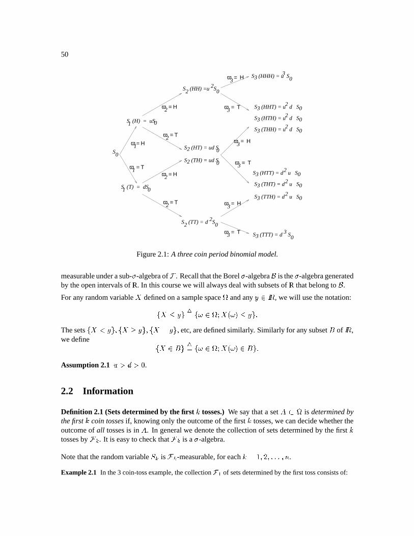
50
S3 (HHH) = u
S3
S3
S3 d S02(HHT) = u
S3
S3
S3
(HH) = u 22S S0
S0
1
1ω = Η
ω = Τ
2
2
2
2 3
3
3
3
3
3
ω = Η
ω = Τ
ω = Η
ω = Τ
ω = Η
ω = Τ
ω = Η
ω = Τ
ω = Η
ω = Τ
S (T) = dS1
S (H) = uS1
0
0
S3 S03(TTT) = d
S03
d S02
d S02
(HTH) = u
(THH) = u
S02
S02
(HTT) = d u
S02
(TTH) = d
(THT) = d u
u
22S S0(TT) = d
2S (TH) = ud S
(HT) = ud S2S
0
0
Figure2.1: A threecoinperiodbinomialmodel.
measurableunderasub- -algebraof . RecallthattheBorel -algebraÝ is the -algebrageneratedby theopenintervalsof IR. In thiscoursewewill alwaysdealwith subsetsof IR thatbelongto Ý .
For any randomvariable
definedonasamplespaceT
andany ¨ ¼ , wewill usethenotation:U Ã ZwtVUl\0¨ TÁ \NÃ Z3RThesetsU Z3)lU r Z3)OU Z:) etc,aredefinedsimilarly. Similarly for any subset of ¼ ,wedefine U ¨M/ZxtVUl\0¨ TÁ \N¨M/Z:RAssumption2.1 . t t $ .2.2 Information
Definition 2.1(Setsdeterminedby the first ] tosses.)We saythata set q T is determinedbythefirst ] coin tossesif, knowing only theoutcomeof thefirst ] tosses,we candecidewhethertheoutcomeof all tossesis in . In generalwe denotethecollectionof setsdeterminedby thefirst ]tossesby ^ . It is easyto checkthat ^ is a -algebra.
Notethattherandomvariable+2^ is ^ -measurable,for each]/%)F)IRERIR:)*à .
Example2.1 In the3 coin-tossexample,thecollection yz of setsdeterminedby thefirst tossconsistsof:
CHAPTER2. ConditionalExpectation 51
1. |3~589358 ,2. |8 ~3388388 ,3. ,
4. .
Thecollection y of setsdeterminedby thefirst two tossesconsistsof:
1. |3 ~/9 ,2. |3 ~/358 ,3. | ~33 ,4. |8_~h83A88 ,5. Thecomplementsof theabove sets,
6. Any unionof theabove sets(includingthecomplements),
7. and .
Definition 2.2(Information carried by a random variable.) Let
bearandomvariableT ð6 ¼ .
We saythata set rq T is determinedby therandomvariable
if, knowing only thevalue d\`
of therandomvariable,wecandecidewhetheror not \ ¨M . Anotherwayof sayingthis is thatforevery ¨W ¼ , either
- q or 2áMr . Thecollectionof susbetsof
Tdetermined
by
is a -algebra,whichwe call the -algebrageneratedby
, anddenoteby J .If therandomvariable
takesfinitely many differentvalues,then J is generatedby thecollec-
tion of sets U - \| ÿ \0¨ T Z Áthesesetsarecalledtheatomsof the -algebra` .In general,if
is a randomvariable
T ð0 ¼ , then h is givenbyh HVU - ) Á ¨jÝPZ3RExample2.2(Setsdeterminedby ) The -algebrageneratedby consistsof thefollowing sets:
1. |3 /9h#] 9 ¡ Xh¢ £ ,2. |8_ h83A883h h¤ £ b3. |3¥¦|§¨ h h¢©¤ £ b4. Complementsof theabove sets,
5. Any unionof theabove sets,
6. ¡ ,7. ¡ ª « .
52
2.3 Conditional Expectation
In orderto talk aboutconditionalexpectation,we needto introducea probabilitymeasureon ourcoin-tosssamplespace
T. Let usdefineD£ ¨q#$)EI is theprobabilityof ? ,D1 tgeP is theprobabilityof A ,D thecoin tossesareindependent,sothat,e.g., ?W?MA(J G ) etc.D #[Zt¬ \ ªK¬ d\a , ®rq T .
Definition 2.3(Expectation.) Ó t ¢\ ª T d\` \alRIf q T then ¬ d\`Zt ² if \ ¨M$ if \¯ ¨Mand Ój# ¬ @ ó ¬ 3 Ù ¢\ ª>¬ \| d\alRWe canthink of Ój# ¬ asapartial averageof
over theset .
2.3.1 An example
Let us estimate+" , given +2G . Denotethe estimateby Ó+" ÿ +2G* . From elementaryprobability, Ój#+" ÿ +2G is a randomvariable& whosevalueat \ is definedby&d\``Q Ój#+" ÿ +2G` l)where + G d\` . Propertiesof Ój#+ ÿ + G :D Ój#+" ÿ +fGl shoulddependon \ , i.e., it is a randomvariable.D If thevalueof +2G is known, thenthevalueof Ój#+" ÿ +2Gl shouldalsobeknown. In particular,
– If \q?@?@? or \£Q?W?MA , then +fG%d\aJ. G +4, . If weknow that +2GKd\aJ. G +-, , thenevenwithoutknowing \ , we know that +N>d\aJ.5+4, . We define Ój#+" ÿ +2GI#?@?@?@2 Ój#+N ÿ +fG*I?W?MA(".;+-,>R
– If \ VAAPA or \0APA[? , then +2GKd\ag G +4, . If we know that +2G>\aa G +-, , thenevenwithoutknowing \ , we know that +N>d\aJ:+-, . Wedefine Ój#+N ÿ +fG*IAPAPA(J Ó+" ÿ +2GllAA(?@J :+-,%R
CHAPTER2. ConditionalExpectation 53
– If \¨qVLU>?MA(?M)*?MAPA[)A(?@?j)AP?MAZ , then +2G%\aP.5:+-, . If we know +fG%d\aP.5:+ , , thenwe do not know whether+ V.5+ , or + :+ , . We thentakea weightedaverage: #[` G n ; G n G n ; G F 5 RFurthermore, ó ¬ +"*: G .;+-,Jn 5 G .5+-,`n G :+-,Jn 5 G 3+-, ; .n6:+-,For \ ¨ we define Ój#+" ÿ +2GId\`` þ ¬/+"*3 #[ G #.pn63w+-,>RThen ó ¬ Ój#+N ÿ +2Gl: ó ¬ +": R
In conclusion,wecanwrite Ó+" ÿ +2G*Ed\|h1òH#+2GId\awl)where òfÍ5" ÎÏÐ ÏÑ
.5+-, if Í. G +-,G #.n6:+ , if Í.;3+ ,3+-, if Í G +-,In otherwords, Ój#+" ÿ +2G is randomonly throughdependenceon +2G . We alsowrite Ój#+" ÿ +2GÍ5J òf#Í;l)whereò is thefunctiondefinedabove.
Therandomvariable Ój#+" ÿ +2G hastwo fundamentalproperties:D Ój#+ ÿ + G is `#+ G -measurable.D For every set V¨j`#+2G , ó ¬ Ój#+" ÿ +2G: Ù ó ¬ +"*: R2.3.2 Definition of Conditional Expectation
PleaseseeWilliams, p.83.
Let T )j) beaprobabilityspace,andlet ¯ beasub- -algebraof . Let
bearandomvariableon T )j)* . Then Ój ÿ ¯2 is definedto beany randomvariable& thatsatisfies:
(a) & is ¯ -measurable,
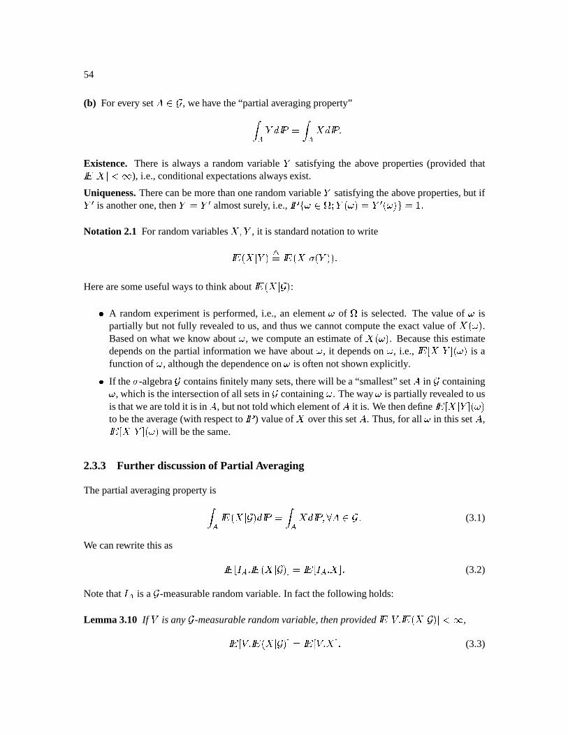
54
(b) For every set ¨M¯ , wehave the“partial averagingproperty”ó ¬ &: ó ¬ 3 RExistence. Thereis alwaysa randomvariable & satisfyingthe above properties(provided that Ó ÿ ÿ 0É ), i.e.,conditionalexpectationsalwaysexist.
Uniqueness.Therecanbemorethanonerandomvariable& satisfyingtheaboveproperties,but if& ! is anotherone,then &¸C& ! almostsurely, i.e., pUl\b¨ TÁ &jd\``b& ! \|Z(ã%RNotation 2.1 For randomvariables
)& , it is standardnotationto write Ój ÿ & t Ój ÿ 2&ïlRHerearesomeusefulwaysto think about Ój ÿ ¯- :D A randomexperimentis performed,i.e., an element\ of
Tis selected.The valueof \ is
partially but not fully revealedto us,andthuswe cannotcomputetheexact valueof d\| .
Basedon whatwe know about \ , we computeanestimateof \| . Becausethis estimate
dependson thepartial informationwe have about \ , it dependson \ , i.e., Ó ÿ &[ed\` is afunctionof \ , althoughthedependenceon \ is oftennot shown explicitly.D If the -algebra containsfinitely many sets,therewill bea“smallest”set in ¯ containing\ , which is theintersectionof all setsin ¯ containing\ . Theway \ is partiallyrevealedto usis thatwearetold it is in , but not told whichelementof it is. Wethendefine Ó ÿ &ed\`to betheaverage(with respectto ) valueof
over thisset . Thus,for all \ in thisset , Ó ÿ &Pd\| will bethesame.
2.3.3 Further discussionof Partial Averaging
Thepartialaveragingpropertyisó ¬ Ój ÿ ¯-3 ó ¬ : )°®¨¯R (3.1)
We canrewrite thisas Ó ¬ R Ój ÿ ¯- Ó ¬ R R (3.2)
Notethat ¬ is a ¯ -measurablerandomvariable.In fact thefollowing holds:
Lemma 3.10 Ifu
is any ¯ -measurablerandomvariable,thenprovided Ó ÿ u R Ój ÿ ¯- ÿ 0É , Ó u R Ó ÿ ¯- Ó u R R (3.3)
CHAPTER2. ConditionalExpectation 55
Proof: To seethis, first use(3.2) andlinearity of expectationsto prove (3.3) whenu
is a simple¯ -measurablerandomvariable,i.e.,u
is of theformu ¬ » ^ f ÷ ^ ¬E± , whereeach ^ is in ¯ and
each÷ ^ is constant.Next considerthecasethatu
is a nonnegative ¯ -measurablerandomvariable,but is not necessarilysimple. Sucha
ucan be written as the limit of an increasingsequence
of simplerandomvariablesu » ; we write (3.3) for each
u » and thenpassto the limit, usingtheMonotoneConvergenceTheorem(SeeWilliams), to obtain (3.3) for
u. Finally, the general -
measurablerandomvariableu
canbewrittenasthedifferenceof twononnegativerandom-variablesu u v u , andsince(3.3)holdsforu v and
u it musthold foru
aswell. Williams callsthisargumentthe“standardmachine”(p. 56).
Basedon this lemma,we canreplacethesecondconditionin thedefinitionof a conditionalexpec-tation(Section2.3.2)by:
(b’) For every ¯ -measurablerandom-variableu
, wehave Ó u R Ój ÿ ¯ Ó u R R (3.4)
2.3.4 Propertiesof Conditional Expectation
PleaseseeWillamsp. 88. Proofsketchesof someof thepropertiesareprovidedbelow.
(a) Ó Ój ÿ ¯-J Ój lRProof:Justtake in thepartialaveragingpropertyto be
T.
Theconditionalexpectationof
is thusanunbiasedestimatorof therandomvariable
.
(b) If
is ¯ -measurable,then Ój ÿ ¯2J RProof:Thepartialaveragingpropertyholdstrivially when & is replacedby
. And since
is ¯ -measurable,
satisfiestherequirement(a)of aconditionalexpectationaswell.
If theinformationcontentof ¯ is sufficientto determine
, thenthebestestimateof
basedon ¯ is
itself.
(c) (Linearity) Ój#Þ n0Þ G G ÿ ¯HhÞ Ój ÿ ¯"2n1Þ G Ój G ÿ ¯"lR(d) (Positivity) If
r0$ almostsurely, then Ój ÿ ¯2r0$«RProof:TakebVUO\¨ TÁ Ój ÿ ¯-ld\a0$Z . Thissetis in ¯ since Ój ÿ ¯2 is ¯ -measurable.Partial averagingimplies þ ¬ Ój ÿ ¯2w3 k þ ¬ : . The right-handsideis greaterthanor equalto zero,and the left-handside is strictly negative, unless (<ý$ . Therefore, #[`$ .
56
(h) (Jensen’s Inequality)If Me:¼ð6¼ is convex and Ó ÿ J ÿ 0É , then Ój)J ÿ ¯2rfJ# Ó ÿ ¯wlRRecalltheusualJensen’s Inequality: ÓN hrfJ# Ój OR
(i) (TowerProperty)If Q is asub- -algebraof ¯ , then Ó Ój ÿ ¯2 ÿ Q<J Ój ÿ QlRQ is asub- -algebraof ¯ meansthat ¯ containsmoreinformationthan Q . If we estimate
basedon theinformationin ¯ , andthenestimatetheestimatorbasedon thesmalleramountof informationin Q , thenwe getthesameresultasif we hadestimated
directly basedon
theinformationin Q .
(j) (Takingoutwhatis known) If d is ¯ -measurable,then Ój)d ÿ ¯2`d[R Ó ÿ ¯ORWhenconditioningon ¯ , the ¯ -measurablerandomvariabled actslike aconstant.
Proof: Let d bea ¯ -measurablerandomvariable.A randomvariable& is Ój)d ÿ ¯f if andonly if
(a) & is ¯ -measurable;
(b) þ ¬ &: Qþ ¬ d : )°®¨¯ .
Take &7²d[R Ój ÿ ¯- . Then & satisfies(a) (a productof ¯ -measurablerandomvariablesis¯ -measurable).& alsosatisfiesproperty(b), aswe cancheckbelow:ó ¬ &3 Ój# ¬ R &/ Ó ¬ d[ Ój ÿ ¯2 Ó ¬ d[R ((b’) withu ¬ d ó ¬ d : R
(k) (Roleof Independence)If Q is independentof `#J l)¯- , then Ó ÿ 2#¯)>QwJ Ój ÿ ¯2lRIn particular, if
is independentof Q , then Ój ÿ Qh Ój lR
If Q is independentof
and ¯ , thennothingis gainedby includingtheinformationcontentof Q in theestimationof
.
CHAPTER2. ConditionalExpectation 57
2.3.5 Examplesfr om the Binomial Model
Recallthat <aVUk")*·)*¹J) T Z . Noticethat Ój#+2G ÿ <* mustbeconstanton · and ¹ .
Now since Ój#+fG ÿ <* mustsatisfythepartialaveragingproperty,ó ¬E³ Ó+2G ÿ : ó ¬³ +2Gl3 )ó ¬E´ Ó+2G ÿ : ó ¬´ +2G3 RWe compute ó ¬ ³ Ój#+ G ÿ : # · lR Ój#+ G ÿ Ed\| Ój#+2G ÿ <Id\al)°®\_¨·ïROntheotherhand, ó ¬E³ +2Gl: G . G +-,`n 5 .5:+-,KRTherefore, Ój#+2G ÿ <*ld\aJ . G +-,`n .5:+-,>)°®\0¨P·/RWe canalsowrite Ó+ G ÿ ld\a . G + , n .;3+ , .pn :.;+-, .pn :+"Id\`l)5®\0¨·Similarly, Ój#+2G ÿ *Ed\|hg .n 3+NOd\`l)°®\¨MP¹`RThusin bothcaseswe have Ó+2G ÿ *ld\aJ .n :+"Id\al)°®\_¨ T RA similarargumentonetimesteplatershowsthat Ój#+4c ÿ GId\aJg .n :+2GKd\alRWe leave the verificationof this equalityasan exercise. We can verify the Tower Property, forinstance,from thepreviousequationswehave Ó Ój#+ c ÿ G ÿ ý Ó .[n 3w+ G ÿ G .n : Ój#+2G ÿ (linearity) .n : G +NiRThisfinal expressionis Ó+-c ÿ .
58
2.4 Martingales
Theingredientsare:D A probabilityspace T )<)* .D A sequenceof -algebras/,>)w<I)IRIRER)p» , with thepropertythat /,xqb<¦qRIRERµqb/»Mq . Suchasequenceof -algebrasis calleda filtration.D A sequenceof randomvariables¶£,>)¶6l)IRERIR5)¶9» . This is calledastochasticprocess.
Conditionsfor a martingale:
1. Each ¶q^ is <^ -measurable.If you know theinformationin ^ , thenyou know thevalueof¶ ^ . WesaythattheprocessUb¶ ^ Z is adaptedto thefiltration UE ^ Z .2. For each] , Ój)¶^ v ÿ /^KJ¶q^ . Martingalestendto goneitherupnordown.
A supermartingaletendstogodown, i.e. thesecondconditionaboveis replacedby Ój)¶^ v ÿ /^>ö ^ ; a submartingaletendsto goup, i.e. Ój)¶ ^ v ÿ ^ rf¶ ^ .Example2.3(Example from the binomial model.) For · (¸75¹ wealreadyshowedthatª º _»¼½z7¾ yS» À¿ ¢ZÁRÂ/¤k _»©ÃFor · Ä , we set y£ Å , the “tri vial -algebra”. This -algebracontainsno information,andanyy £ -measurablerandomvariablemustbeconstant(nonrandom).Therefore,by definition, ª º z ¾ y £ is thatconstantwhichsatisfiestheaveragingpropertyó ª º ½z7¾ y£ A¤bª Æh ó ½z ¤kª Æ ÃTheright handsideis ª º ½z Ç¿ ¢ZÁÈÂ/¤b £ , andsowehaveª º z ¾ y £ X À¿ ¢ZÁRÂ/¤b £ ÃIn conclusion,É
If Ç¿ ¢ZÁMÂ/¤b Ef¸ then _» yZ»_9· ĸ75¹5Êb is a martingale.É
If Ç¿ ¢ZÁMÂ/¤b Ë̸ then » y » 9· ĸ75¹5Êb is a submartingale.É
If Ç¿ ¢ZÁMÂ/¤b Í̸ then » y » 9· ĸ75¹5Êb is a supermartingale.
Chapter 3
Arbitrage Pricing
3.1 Binomial Pricing
Returnto thebinomialpricingmodel
Pleasesee:Î Cox,RossandRubinstein,J. FinancialEconomics, 7(1979),229–263,andÎ CoxandRubinstein(1985),Options Markets, Prentice-Hall.
Example3.1(Pricing a Call Option) SupposeÏÑÐ ¹Ò5Ó Ð Ä Ã Ô Ò9Õ Ð ¹ ÔÖ (interestrate), ×ئÐ+Ô Ä . (In thisandall examples,theinterestratequotedis perunit time,andthestockprices ×Ø Ò ×½Ù Ò ÃÃà areindexedby thesametimeperiods).We know that × Ù/ÚÜÛÝ Ð+Þ ¸Ä7Ä if Û8Ù Ðhß¹ Ô if Û8Ù ÐàFind thevalueat timezero of a call optionto buy oneshareof stockat time 1 for $50(i.e. thestrikeprice is$50).
Thevalueof thecall at time1 isá Ù ÚâÛÝ Ð Ú ×½Ù ÚÜÛ¡ÝEã Ô Ä Ý ¼ Ð+Þ Ô Ä if Û ÙÐßÄ if Û ÙÐÈàSupposetheoptionsellsfor $20at time0. Let usconstructa portfolio:
1. Sell 3 optionsfor $20each.Cashoutlayis ã§äå Ä Ã2. Buy 2 sharesof stockfor $50each.Cashoutlayis $100.
3. Borrow $40.Cashoutlayis ã3äæ Ä Ã59
60
Thisportfolio thusrequiresnoinitial investment.For this portfolio, thecashoutlayat time 1 is:Û Ù¡Ðhß Û Ù¡ÐàPay off option äç Ô Ä ä ÄSell stock ã3ä ¹Ä7Ä ã3ä Ô ÄPay off debt ä Ô Ä ä Ô ÄãMãÈãMãÈã ãÈãRã]ãRãä Ä ä Ä
Thearbitragepricing theory(APT)valueof theoptionat time 0 isá Ø8Ð ¹Ä .
AssumptionsunderlyingAPT:Î Unlimitedshortsellingof stock.Î Unlimitedborrowing.Î No transactioncosts.Î Agentis a “small investor”,i.e.,his/hertradingdoesnot move themarket.
Important Observation: TheAPT valueof theoptiondoesnot dependon theprobabilitiesof èand é .
3.2 Generalone-stepAPT
Supposea derivative securitypaysoff the amount êXë at time 1, where êë is an ìíë -measurablerandomvariable. (This measurabilityconditionis important;this is why it doesnot makesenseto usesomestockunrelatedto the derivative securityin valuing it, at leastin the straightforwardmethoddescribedbelow).Î Sell thesecurityfor ê½î at time0. ( êµî is to bedeterminedlater).Î Buy ïî sharesof stockat time 0. ( ïî is alsoto bedeterminedlater)Î Invest ê½î¦ðKïîñEî in the money market,at risk-free interestrate ò . ( ê½îð+ïî/ñEî might be
negative).Î Thenwealthat time1 is ó ëõôö ïî7ñë¡÷ø°ù÷(òbú7ø)ê½î3ðOïîñEî7úö ø5ù3÷òbú>ê½î8÷ïî©ø)ñë8ðKø°ù÷(òbú>ñEî/ú/ûÎ Wewantto chooseê î and ï î sothat ó ë ö êë
regardlessof whetherthestock goesupor down.
CHAPTER3. ArbitragePricing 61
Thelastconditionabove canbeexpressedby two equations(which is fortunatesincetherearetwounknowns): ø5ù8÷fòbú>ê½î¡÷(ïî!øNñëkø)èÈúðfø5ù3÷òbú>ñEî/ú ö êëkø)èÈú (2.1)ø5ù3÷òbú>ê½î8÷ïî©ø)ñë7øüéSú§ðfø5ù3÷òbú>ñEî/ú ö êëkøüéSú (2.2)
Note that this is wherewe usethe fact that the derivative securityvalue êEý is a function of ñXý ,i.e., when ñXý is known for a given þ , êEý is known (andthereforenon-random)at that þ aswell.Subtractingthesecondequationabove from thefirst givesïî ö êë7ø)èÈúðOêëøÿéSúñ ë ø)èÈúðOñ ë øüéSú û (2.3)
Plugtheformula(2.3)for ïî into (2.1):ø5ù3÷òbú>ê½î ö êëkø)èÈú¡ðïî©ø)ñë7ø)èÈú¡ðfø°ù3÷òbú>ñEî/úö ê ë ø)èÈú¡ð êë7ø)èÈúðOêëøÿéSúøð ú>ñEî øðùZðhòbú>ñ îö ùíð øð ú>êëø)èÈúðKø)êëø)èÈúðOêë7øüéSú>úøðùZðòbúö ù3÷fò ð Ñð êëø)èÈúE÷ ð(ùZðòíð êëøüé ú/ûWe have alreadyassumed . We now alsoassume
ù3÷(ò (otherwisetherewouldbeanarbitrageopportunity).Define ôö ù3÷ò ð ð ôö ðùðòð ûThen
and . Since
÷ ö ù , we have ù and ö ù ð . Thus,
arelikeprobabilities.We will returnto this later. Thusthepriceof thecall at time0 is givenbyê î ö ùù8÷(ò ê ë ø)èÈúE÷ ê ë øüé ú9û (2.4)
3.3 Risk-Neutral Probability Measure
Let bethesetof possibleoutcomesfrom coin tosses.Constructaprobabilitymeasure on by theformula ÑøaþZë þ û7û7û þ©úôö ! "$# þ%'&)(+* ,! "$# þ%'&)-.* is calledtherisk-neutral probabilitymeasure. We denoteby / theexpectationunder . Equa-tion 2.4says ê î ö / 0 ùù?÷fò ê ë21 û
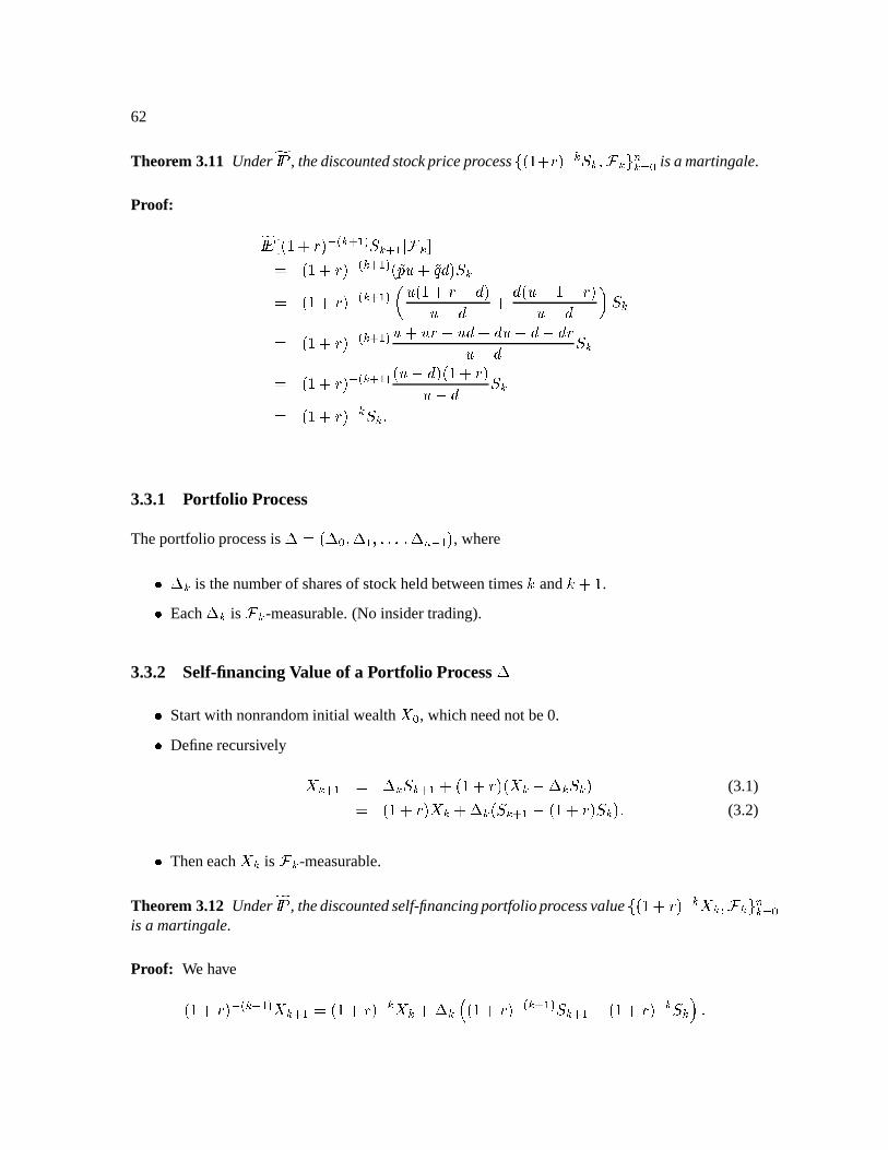
62
Theorem 3.11 Under , thediscountedstockpriceprocess3ø5ù÷òkú54 ý ñXý ìý76 ý & î is a martingale.
Proof: / ø5ù8÷òkú 4.8 ý$9Xë;: ñXý$9ë=< ìý>ö ø5ù8÷fòbú 4?8 ý@9ëA: ø ÷ ú>ñXýö ø5ù8÷fòbú 4?8 ý@9ëA: 0 ¡ø°ù÷(òZð úð ÷ øð(ù<ðhòbúíð 1 ñXýö ø5ù8÷fòbú 4?8 ý@9ëA: ÷B½òSðC ÷ ð ð òð ñýö ø5ù8÷fòbú 4?8 ý@9ëA: øð ú7ø5ù8÷òbúð ñXýö ø5ù8÷fòbú 4 ý ñXýû3.3.1 Portf olio Process
Theportfolio processis ï ö ø)ïî ïíë û7û7û ïD 4 ë°ú , whereÎ ïý is thenumberof sharesof stockheldbetweentimes E and E¦÷+ù .Î Eachïý is ìý -measurable.(No insidertrading).
3.3.2 Self-financingValue of a Portf olio ProcessFÎ Startwith nonrandominitial wealth
ó î , whichneednot be0.Î Definerecursively ó ý$9ë ö ïý7ñý@9ë÷ø°ù3÷òbú7ø ó ýðhïý7ñXýú (3.1)ö ø5ù3÷òbú ó ý ÷ï ý øNñ ý@9ë ð+ø5ù8÷fòbú>ñ ý ú/û (3.2)Î Theneach
ó ý is ìý -measurable.
Theorem 3.12 Under , thediscountedself-financingportfolioprocessvalue 3¨ø5ù8÷(òkú54 ý ó ý ì ý 6 ý & îis a martingale.
Proof: We haveø5ù8÷fòbú$4?8 ý@9ëA: ó ý$9ë ö ø5ù?÷òkú 4 ý ó ý3÷(ïýHGø5ù?÷òkú 4.8 ý$9Xë;: ñXý$9ë3ðKø5ù8÷fòbú 4 ý ñXý>Iû
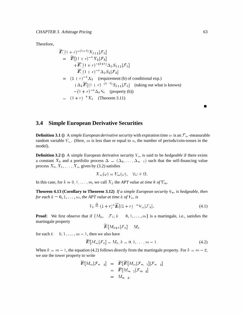
CHAPTER3. ArbitragePricing 63
Therefore, / ø5ù8÷òbú 4?8 ý$9ëA: ó ý@9ë,< ìý$ö / ø5ù8÷òbú 4 ý ó ýJ< ìý5÷H / ø°ù÷(òbú 4?8 ý$9ëA: ïýbñXý$9Xë,< ìý5ðK / ø°ù÷(òbú 4 ý ïýñXýJ< ìý5ö ø5ù3÷òbú 4 ý ó ý (requirement(b) of conditionalexp.)÷¦ïý / ø5ù8÷fòbú 4?8 ý@9ëA: ñXý$9Xë,< ìý5 (takingout whatis known)ðø5ù?÷fòbú 4 ý ïýñXý (property(b))ö ø5ù3÷òbú 4 ý ó ý (Theorem3.11)
3.4 SimpleEuropeanDerivativeSecurities
Definition 3.1() A simpleEuropeanderivativesecuritywith expirationtime L isan ìDM -measurablerandomvariable ê)M . (Here, L is lessthanor equalto , thenumberof periods/coin-tossesin themodel).
Definition 3.2() A simpleEuropeanderivative security ê)M is saidto behedgeableif thereexistsa constant
ó î anda portfolio processï ö ø)ïî ûû7û ïDM 4 ëú suchthat the self-financingvalueprocess
ó î ó ë û7û7û ó M givenby (3.2)satisfiesó M øþ<ú ö ê M øþ3ú ON þQPRwûIn thiscase,for E ö ù û7ûû L , we call
ó ý theAPTvalueat time E of ê M .
Theorem 4.13(Corollary to Theorem 3.12) If a simpleEuropeansecurity ê)M is hedgeable,thenfor each E ö ù û7û/û L , theAPTvalueat time E of ê M isêEý¦ôö ø°ù3÷òbú ý / ø5ù3÷òbú 4 M ê)MS< ìý59û (4.1)
Proof: We first observe that if 3,Thý ìýVU@E ö ù ûû/û L6 is a martingale,i.e., satisfiesthemartingaleproperty / TOý$9ë,< ìý$ ö Thýfor eachE ö ù ûû/û Lðù , thenwe alsohave / TWMS< ìý$ ö Thý E ö ù ûû/û Lðùû (4.2)
When E ö L²ðù , theequation(4.2)followsdirectly from themartingaleproperty. For E ö L²ðRX ,weusethetowerpropertyto write / T M < ì M 4 ö / / T M < ì M 4 ë '< ì M 4 ö / TWM 4 ë,< ìDM 4 Yö TWM 4 û
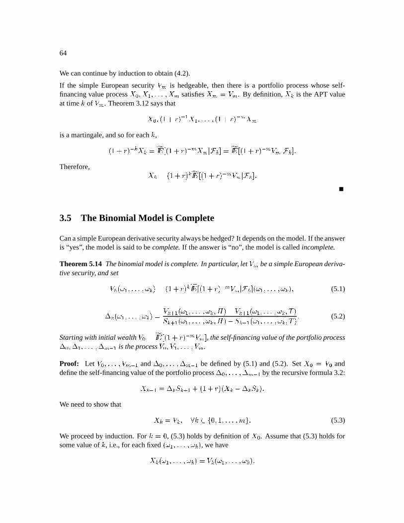
64
We cancontinueby inductionto obtain(4.2).
If the simple Europeansecurity ê M is hedgeable,then there is a portfolio processwhoseself-financingvalueprocess
ó î ó ë ûû7û ó M satisfies
ó M ö êM . By definition,
ó ý is theAPT valueat time E of ê)M . Theorem3.12saystható î ø5ù¡÷(òbú 4 ë ó ë û7ûû ø5ù8÷òbú 4 M ó Mis amartingale,andsofor eachE ,ø5ù3÷òbú$4 ý ó ý ö / ø5ù3÷òbú$4 M ó MS< ìý$ ö / ø5ù8÷fòbú$4 M ê)MS< ìý>5ûTherefore,
ó ý ö ø5ù8÷fòbú ý / ø°ù÷(òbú 4 M ê)MS< ìxýZ9û3.5 The Binomial Model is Complete
CanasimpleEuropeanderivativesecurityalwaysbehedged?It dependsonthemodel.If theansweris “yes”, themodelis saidto becomplete. If theansweris “no”, themodelis calledincomplete.
Theorem 5.14 Thebinomialmodelis complete. In particular, let ê)M bea simpleEuropeanderiva-tivesecurity, andsetêEý©øþ3ë û7ûû þýú ö ø5ù3÷òbú ý / ø5ù8÷òbú$4 M ê)MS< ìý$°øaþ3ë ûû7û þ8ý7ú (5.1)
ïý©øaþ3ë ûû7û þ8ý7ú ö ê ý@9ë øþ ë û7û7û þ ý èÈúXðê ý$9ë øþ ë ûû7û þ ý éSúñXý$9ë!øþ?ë û7û7û þý èÈúXðñý@9ë!øaþ3ë û7ûû þ8ý é ú û (5.2)
Startingwith initial wealth ê î ö / ø5ù8÷fòbú 4 M ê M , theself-financingvalueof theportfolio processïî ïíë ûû7û ïDM 4 ë is theprocessê½î êë û7ûû ê)M .
Proof: Let ê î û7û7û ê M 4 ë and ï î ûû7û ï M 4 ë be definedby (5.1) and(5.2). Set
ó î ö ê î anddefinetheself-financingvalueof theportfolio processïî û7ûû ïDM 4 ë by therecursiveformula3.2:ó ý$9ë ö ïýñXý@9ë¡÷rø5ù8÷fòbú7ø ó ýðïýkñý7ú/ûWe needto show that ó ý ö êý [N E\P]3, ù û7û/û L6_û (5.3)
We proceedby induction.For E ö , (5.3)holdsby definitionof
ó î . Assumethat(5.3)holdsforsomevalueof E , i.e., for eachfixed øþ3ë û7û7û þý7ú , we haveó ý_øþ3ë û7û7û þý7ú ö êEýøþ3ë û7û7û þý7úû
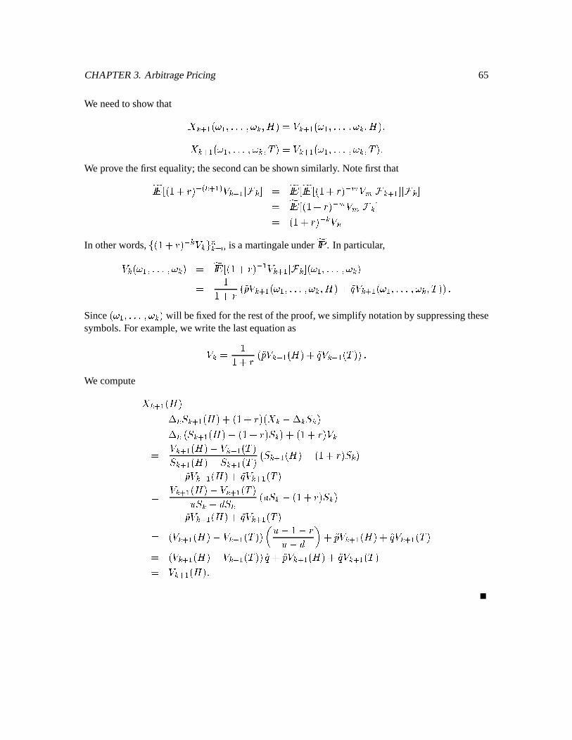
CHAPTER3. ArbitragePricing 65
We needto show that ó ý$9Xëkøaþ3ë û7ûû þ8ý èÈú ö êEý@9ë7øþ3ë û7û7û þý èÈú ó ý$9ëkøþ3ë ûû7û þý éSú ö êEý@9ë7øþ3ë û7û7û þý éSú/ûWe prove thefirst equality;thesecondcanbeshown similarly. Notefirst that / ø5ù8÷òbú$4?8 ý$9ëA: êEý$9Xë,< ìý5 ö / / ø5ù8÷òbú$4 M êM^< ìý$9ë2'< ìý$ö / ø°ù÷òbú$4 M ê)MS< ìý5ö ø5ù?÷òkú 4 ý êEýIn otherwords, 3¨ø5ù3÷òbú$4 ý êý=6 ý & î is a martingaleunder . In particular,êEý©øþ3ë û7ûû þýú ö / ø5ù8÷òbú 4 ë êEý@9ë,< ìý5°øþ3ë ûû7û þý7úö ùù3÷(ò ø êEý$9Xëkøaþ3ë ûû7û þ8ý èÈúE÷ êEý@9ëkøþ3ë û7ûû þý éSú>ú½ûSince øþ3ë ûû7û þý/ú will befixedfor therestof theproof,wesimplify notationby suppressingthesesymbols.For example,wewrite thelastequationasêý ö ùù3÷ò ø êEý@9ëkø)èÈúE÷ êEý@9ëkøüéSú#úEûWe compute ó ý@9ëkø)èÈúö ï ý ñ ý@9ë ø)èÈúE÷¯ø°ù÷(òbú7ø ó ý ðï ý ñ ý úö ïýøüñXý@9ëkø)èÈúðKø°ù÷(òbú>ñXý/úX÷rø5ù8÷fòbú>êEýö êEý$9ëkø)èÈú¡ðêEý$9ëkøüéSúñXý$9ëkø)èÈú¡ðñý@9ë!øÿéSú øNñXý@9ëkø)èÈúðKø°ù÷(òbú>ñXý/ú÷ ê ý$9ë ø)èÈú÷ ê ý$9Xë øÿéSúö êEý@9ëkø)èÈúðêEý@9ëkøüé ú½ñXýZð ñý ø_½ñXý ðfø5ù3÷òbú>ñXýú÷ êEý$9ëkø)èÈú÷ êEý$9XëkøÿéSúö øüêEý@9ëkø)èÈúðOêEý$9XëkøÿéSú>ú 0 ðùðOòð 1 ÷ êEý@9ëkø)èÈúE÷ êEý@9ëkøüéSúö øüêEý@9ëkø)èÈúðOêEý$9XëkøÿéSú>ú ÷ êý$9ëkø)èÈúE÷ êEý@9ëkøüéSúö êEý@9ëkø)èÈú/û

66
Chapter 4
The Mark ov Property
4.1 Binomial Model Pricing and Hedging
Recall that ê M is the givensimpleEuropeanderivative security, andthe valueandportfolio pro-cessesaregivenby:êEý ö ø5ù3÷òbú ý / ø5ù8÷òkú54 M êMD< ìý$ E ö ù û7û/û L ð(ùûïý_øþ3ë ûû7û þý7ú ö êEý$9Xëkøaþ3ë û7ûû þ8ý èÈúðOêEý@9ë7øþ3ë û7û7û þý éSúñý@9ë!øaþ3ë û7ûû þ8ý èÈúðOñXý$9ëkøþ3ë ûû7û þý éSú E ö ù ûû/û LðfùûExample4.1(Lookback Option) ÏÐ ¹Ò5Ó ÐB`VaÔ Ò9Õ ÐQ`ba ¹ Ô Ò × Ø Ð æ ÒZcd Ð ÙfehgYikjl ikj Ðm`VaÔ Ò$cn Ð ç8ã cd ÐB`VaÔbaConsidera simpleEuropeanderivativesecuritywith expiration2, with payoff givenby (SeeFig. 4.1):áVo ÐqpDr>sØYtJuvt o Ú × uZã Ô Ý e aNoticethat áVo Ú ßß Ý Ð çç Ò áVo Ú ßà Ý Ðxw^yÐ áVo Ú à3ß Ý Ðx` Ò áVo Ú à8à Ý Ðz`baThepayoff is thus“path dependent”.Workingbackwardin time,wehave:á Ù Ú ß Ý Ð çç| Õ? cd á o Ú ßß Ý~ cn á o Ú ßà Ý Ð æ Ô `VaÔK ç7ç| `ba ÔKSw ÐhÔVa å ` Òá Ù Ú à Ý Ð æ Ô `VaÔK` `VaÔK` Ðx` Òá Ø Ð æ Ô `ba ÔKxÔba å ` `baÔ+` Ð ¹ a ¹ æ aUsingthesevalues,wecannow compute: Ø Ð á ÙÚ ß Ý ã á ÙÚ à Ý×½Ù Ú ß Ý ã ×½Ù Ú à Ý Ðx`Vavw Ò ÙÚ ß Ý Ð á=o Ú ßß Ý½ã áVo Ú ßà Ý× o Ú ßß Ý½ã × o Ú ßà Ý Ðz`ba åv Ò
67
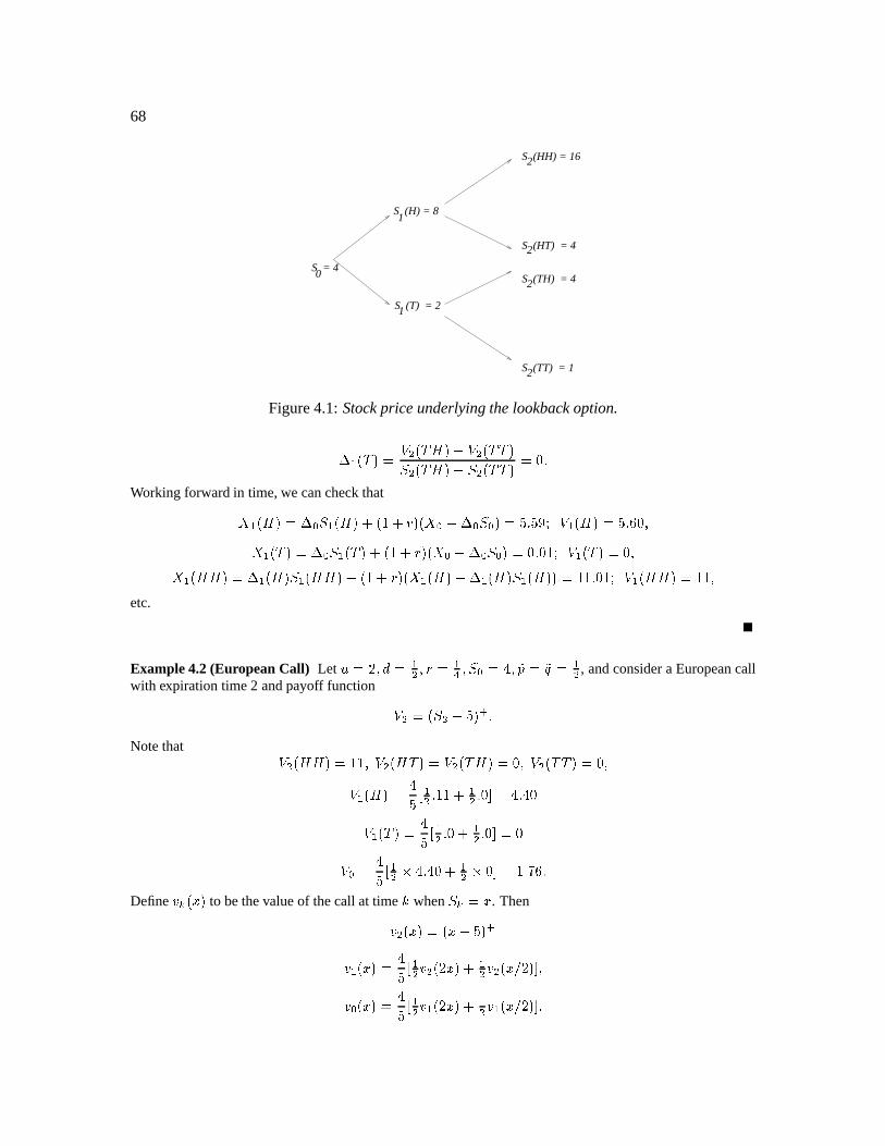
68
S = 40
S (H) = 8
S (T) = 2
S (HH) = 16
S (TT) = 1
S (HT) = 4
S (TH) = 4
1
1
2
2
2
2
Figure4.1: Stock priceunderlyingthelookback option. ÙÚ à Ý Ð á o Ú à3ß Ý½ã á o Ú à8à Ý× o Ú à3ß Ý½ã × o Ú à8à Ý Ðz`baWorking forwardin time,wecancheckthat Ù/Ú ß Ý Ð Ø × Ù/Ú ß Ý~hÚç| Õ Ý>Ú Ø§ã Ø × Ø/Ý ÐhÔVaÔvV á ÙÚ ß Ý ÐhÔVa å ` Ò Ù/Ú à Ý Ð Ø × Ù/Ú à Ý)ÚAç| Õ Ý#Ú Øã Ø × ØÝ Ðz`ba ` ç á ÙÚ à Ý ÐC` Ò ÙÚ ßß Ý Ð ÙÚ ß Ý × ÙÚ ßß ÝÚAç| Õ Ý>Ú Ù/Ú ß Ý½ã ÙÚ ß Ý × ÙÚ ß ÝAÝ Ð ç7ç a` ç á Ù/Ú ßß Ý Ð ç7ç Òetc.
Example4.2(EuropeanCall) Let ÏÐ ¹Ò9Ó Ð Ùo Ò5Õ Ð Ù Ò × Ø Ð æ Òvcd Ð cn Ð Ùo , andconsidera Europeancallwith expirationtime2 andpayoff function á=o Ð Ú × o ã Ô Ý e aNotethat á o Ú ßß Ý Ð ç7ç Ò á o Ú ßà Ý Ð á o Ú à3ß Ý ÐC` Ò á o Ú à8à Ý Ðx` Òá Ù Ú ß Ý Ð æ Ô Ùo a ç7ç? Ùo a` Ð æ a æ `á Ù Ú à Ý Ð æ Ô Ùo a` Ùo a ` Ðx`á Ø Ð æ Ô Ùo æ a æ ` Ùo S` Ð ç a 7å aDefine $u Ú__Ý to bethevalueof thecall at time when ×huZÐ . Then o Ú©Ý Ð Ú ã Ô Ý eÙ Ú©Ý Ð æ Ô Ùo o Ú ¹ ©Ý~ Ùo o Ú_h ¹ Ý Ò Ø/Ú©Ý Ð æ Ô Ùo Ù/Ú ¹ ©Ý~ Ùo Ù/Ú_h ¹ Ý a
CHAPTER4. TheMarkov Property 69
In particular, o ÚAçå7Ý Ð ç7ç Ò o Ú&æbÝ Ðz` Ò o ÚçÝ Ðz` ÒÙ Ú7Ý Ð æ Ô Ùo a çç. Ùo a` Ð æ a æ ` Ò ÙÚ ¹ Ý Ð æ Ô Ùo a` Ùo a` Ðz` Ò/Ø8Ð æ Ô Ùo æ a æ ` Ùo S` Ð ç a 7å a
Let u©Ú__Ý bethenumberof sharesin thehedgingportfolio at time when × u Ð . Then u©Ú©Ý Ð u5e½Ù/Ú ¹ ©Ý½ã u5e½Ù/Ú_h ¹ ݹ ã\J ¹ Ò ¦ÐW` Ò ç a4.2 Computational Issues
For a model with periods(coin tosses), has X elements.For period E , we must solve X ýequationsof theformêý_øþ3ë û7û7û þý7ú ö ùù3÷ò êEý@9ë7øþ3ë û7û7û þý èÈú÷ êEý$9Xëkøaþ3ë ûû7û þ8ý é ú9ûFor example,a three-monthoptionhas66 tradingdays.If eachdayis takento beoneperiod,then öV and X72DOùv ëf .Therearethreepossiblewaysto dealwith thisproblem:
1. Simulation.Wehave, for example,thatê½î ö ø5ù?÷òkú 4 /ê andso we could computeê î by simulation. More specifically, we could simulate cointossesþ ö øþ3ë ûû7û þ©ú underthe risk-neutralprobability measure.We could storethevalueof ê)øþ<ú . We could repeatthis several timesandtakethe averagevalueof ê) asanapproximationto /ê) .
2. Approximatea many-periodmodelby a continuous-timemodel. Thenwe canusecalculusandpartialdifferentialequations.We’ll getto that.
3. Look for Markov structure.Example4.2hasthis. In period2, theoptionin Example4.2hasthreepossiblevalues,ø°ù ú ,ø©ú ,ø5ù7ú , ratherthanfourpossiblevaluesê?køNè]èÈú ê?øNèMé ú ê?/øüéSèÈú ê./øüééSú .If therewere66periods,thenin period66therewouldbe67possiblestockpricevalues(sincethefinal pricedependsonly onthenumberof up-ticksof thestockprice– i.e.,heads– sofar)andhenceonly 67possibleoptionvalues,ratherthan X 2 Dhù ëf .
70
4.3 Mark ov Processes
Technicalcondition alwayspresent:Weconsideronly functionson IR andsubsetsof IR which areBorel-measurable,i.e.,weonly considersubsets of IR thatarein andfunctions Ñeh ¡£¢B ¡ suchthat ?4 ë is a function +¢x .
Definition 4.1() Let ø ì 2¤ ú bea probabilityspace.Let 37ìý=6 ý & î bea filtration under ì . Let3 ó ý=6 ý & î bea stochasticprocesson ø ì Y¤ ú . Thisprocessis saidto beMarkovif:Î Thestochasticprocess3 ó ý76 is adaptedto thefiltration 3ìý=6 , andÎ (TheMarkovProperty).For eachE ö ù ûû/û íðfù , thedistributionof
ó ý@9ë conditionedon ìÑý is thesameasthedistributionof
ó ý@9ë conditionedon
ó ý .4.3.1 Differ ent waysto write the Mark ov property
(a) (Agreementof distributions).For every P¥ ôö ¦ø ¡¦ú , wehave ø ó ý$9ë¦PRD< ìý7ú ö / $§3ø ó ý$9ëú< ìý>ö / $§3ø ó ý$9ëú< ó ýYö ó ý@9ë¦PRD< ó ýY5û(b) (Agreementof expectationsof all functions).For every(Borel-measurable)function ¨MeV ¡£¢m ¡
for which /\<¨ø ó ý$9Xëúv<hQ© , wehave / ¨ø ó ý$9ëú< ìxý5 ö / ¨¡ø ó ý$9ë°úv< ó ýY9û(c) (Agreementof Laplacetransforms.)For every PR ¡ for which /DªZ« ó ý@9ë Q© , wehave
/¬ª « ó ý$9ë®®®® ìý5¯ ö /¬_ª « ó ý$9Xë)®®®®ó ý$¯Sû
(If wefix anddefine¡ø°½ú ö ª «>± , thentheequationsin (b) and(c) arethesame.Howeverin(b) wehaveaconditionwhichholdsfor everyfunction ¨ , andin (c) weassumethisconditiononly for functions of theform ¨ø°µú ö ª «>± . A mainresultin thetheoryof Laplacetransformsis thatif theequationholdsfor every ¨ of thisspecialform, thenit holdsfor every ¨ , i.e., (c)implies(b).)
(d) (Agreementof characteristicfunctions)For every \PR ¡ , we have /³²´ªZµ « ó ý@9ë < ìýv¶ ö /·²´ª>µ « ó ý$9Xë < ó ý>¶ where ö¹ ð¦ù . (Since <ª µ «>± < ö <;º>»b¼k°?÷ ¼2½´¾¦°!< ù wedon’t needto assumethat /\<ª µ «>± <~© .)
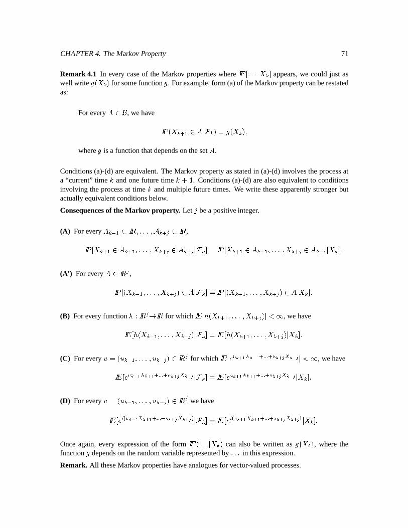
CHAPTER4. TheMarkov Property 71
Remark 4.1 In every caseof the Markov propertieswhere / û7ûû@< ó ý5 appears,we could just aswell write ¡ø ó ý ú for somefunction . For example,form (a)of theMarkov propertycanberestatedas:
For every ¿P\ , wehave ø ó ý@9ë¦PS< ìýú ö ø ó ý/ú where is a functionthatdependsontheset .
Conditions(a)-(d)areequivalent. TheMarkov propertyasstatedin (a)-(d) involvestheprocessata “current” time E andonefuture time E÷rù . Conditions(a)-(d)arealsoequivalentto conditionsinvolving theprocessat time E andmultiple future times. We write theseapparentlystrongerbutactuallyequivalentconditionsbelow.
Consequencesof the Mark ov property. Let À bea positiveinteger.
(A) For every ý@9ë¦ÁQ ¡ û7ûû Y ý@9 " ÁQ ¡ , ó ý$9ë¦PR ý@9ë ûû7û ó ý$9 " PRSý$9 " < ìý5 ö ó ý$9XëÃPRSý$9ë ûû7û ó ý$9 " PSý$9 " < ó ý$9û(A’) For every ¿PR ¡ " , ø ó ý$9ë û7û7û ó ý$9 " úPRS< ìý5 ö ø ó ý$9ë û7ûû ó ý$9 " úPRD< ó ý59û(B) For every function ¨ReJ ¡ " ¢m ¡ for which /\<¨ø ó ý$9ë û7û7û ó ý$9 " ú<hQ© , we have / ¨¡ø ó ý@9ë ûû7û ó ý$9 " ú< ìxý5 ö / ¨¡ø ó ý$9ë û7ûû ó ý$9 " ú< ó ýY5û(C) For every ö øµý$9ë ûû7û ½ý@9 " úKPR ¡ " for which /\<ª «Ä;ÅhÆfÇÄ;ÅhÆ 9ÉÈÈÈ 9 «Ä;Å % ÇÊÄ;Å % <hm© , wehave / ª « Ä;ÅhÆ Ç Ä;ÅhÆ 9ÉÈÈÈ 9 « Ä;Å % Ç Ä;Å % < ìý5 ö / ª « Ä;ÅhÆ Ç Ä;ÅhÆ 9|ÈÈÈ 9 « Ä;Å % Ç ÄAÅ % < ó ý59û(D) For every ö øµý$9ë ûû7û ½ý@9 " úKPR ¡ " wehave
/ ª µ 8 « Ä;ÅhÆ Ç Ä;ÅhÆ 9|ÈÈÈ 9 « Ä;Å % Ç ÄAÅ % : < ìý5 ö / ª µ 8 « Ä;ÅhÆ Ç Ä;ÅhÆ 9|ÈÈÈ 9 « Ä;Å % Ç Ä;Å % : < ó ýY9ûOnceagain,every expressionof the form /Bø5û7ûû@< ó ýú can also be written as ¡ø ó ý/ú , wherethefunction dependson therandomvariablerepresentedby ûû7û in thisexpression.
Remark. All theseMarkov propertieshave analoguesfor vector-valuedprocesses.
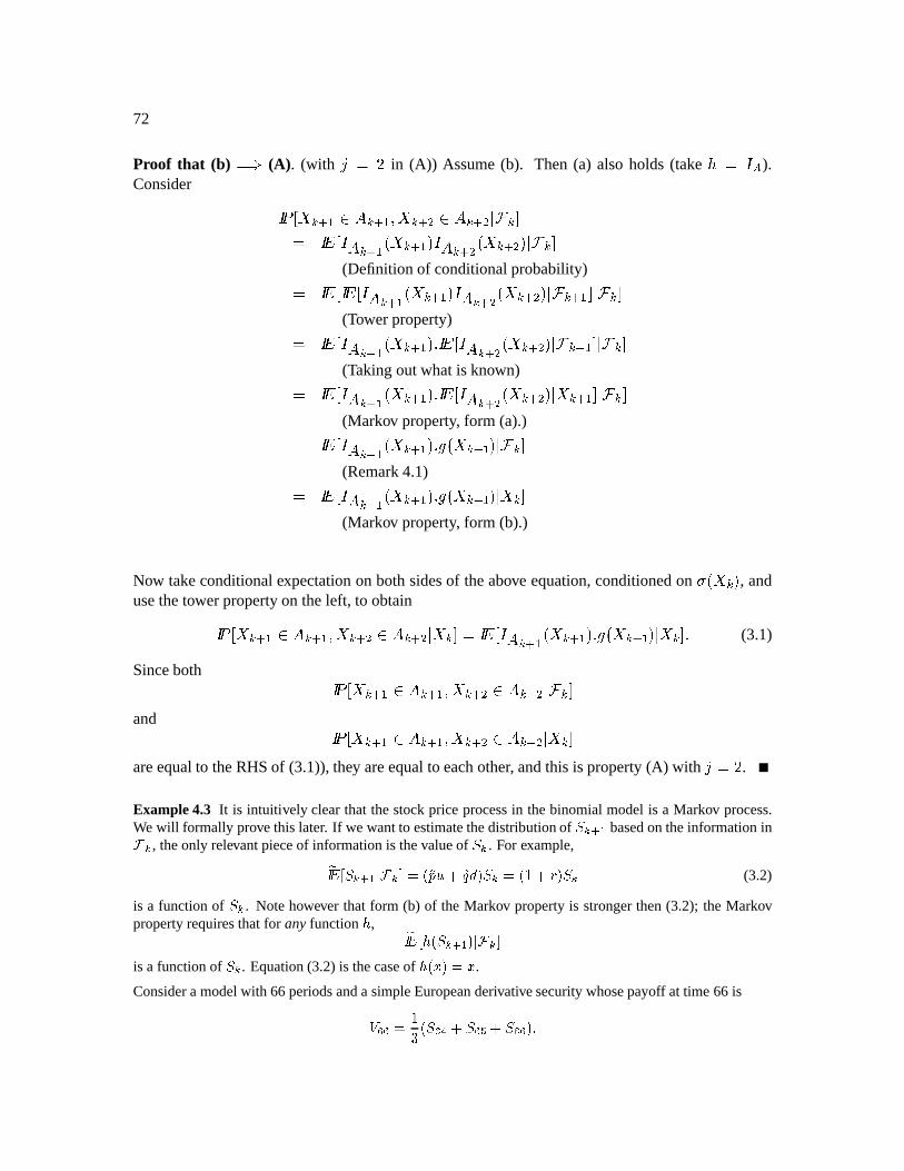
72
Proof that (b) ö?Ë (A). (with À ö X in (A)) Assume(b). Then(a) alsoholds (take ¨ ö $§ ).Consider ó ý$9ë¦PR ý@9ë ó ý@9?ÃPR ý@9?J< ìý5ö / ý@9ë ø ó ý$9ë ú2 ý$9? ø ó ý$9. úv< ì ý
(Definitionof conditionalprobability)ö / / ý@9ë ø ó ý$9XëúY Sý$9? ø ó ý@9?/ú< ìxý$9XëY'< ìý>(Towerproperty)ö / ý@9ë ø ó ý$9ë ú/ûÌ / ý@9? ø ó ý$9. ú< ì ý$9ë '< ì ý (Takingoutwhatis known)ö / ý@9ë ø ó ý$9ëú/ûÌ / ý@9? ø ó ý$9.ú< ó ý@9ë;'< ìýZ(Markov property, form (a).)ö / ý@9ë ø ó ý$9ëú/û ¡ø ó ý$9Xë5ú< ìý$(Remark4.1)ö / ý@9ë ø ó ý$9ëú/û ¡ø ó ý$9Xë5ú< ó ýY(Markov property, form (b).)
Now takeconditionalexpectationon bothsidesof theabove equation,conditionedon Í3ø ó ý/ú , andusethetowerpropertyon theleft, to obtain ó ý@9ë£PR ý@9ë ó ý@9?ÃPR ý@9?V< ó ý5 ö / ý@9ë ø ó ý$9ëú/û ¡ø ó ý$9ë9ú< ó ýY5û (3.1)
Sinceboth ó ý@9ë¦PR ý$9Xë ó ý$9.ÃPR ý$9.h< ìxýZand ó ý$9ëÎPR ý$9Xë ó ý$9.ÃPR ý$9.V< ó ý$areequalto theRHSof (3.1)),they areequalto eachother, andthis is property(A) with À ö X .Example4.3 It is intuitively clearthat thestockpriceprocessin thebinomialmodelis a Markov process.We will formally provethis later. If wewantto estimatethedistributionof × u>e½Ù basedontheinformationinÏ u , theonly relevantpieceof informationis thevalueof × u . For example,ÐÑ º × u>e½ÙÒ Ï u> Ð Ú cd Ï cn Ó Ý × u Ð ÚAç| Õ Ý × u (3.2)
is a functionof ×hu . Notehowever that form (b) of the Markov propertyis strongerthen(3.2); the Markovpropertyrequiresthatfor anyfunction Ó , ÐÑ º Ó Ú ×hu>e½Ù Ý$Ò Ï u is a functionof × u . Equation(3.2) is thecaseof Ó Ú__Ý Ð .Considera modelwith 66periodsanda simpleEuropeanderivativesecuritywhosepayoff at time 66 isá=Ô;Ô Ð çw Ú × Ô × Ô;Õ × Ô;Ô Ý a
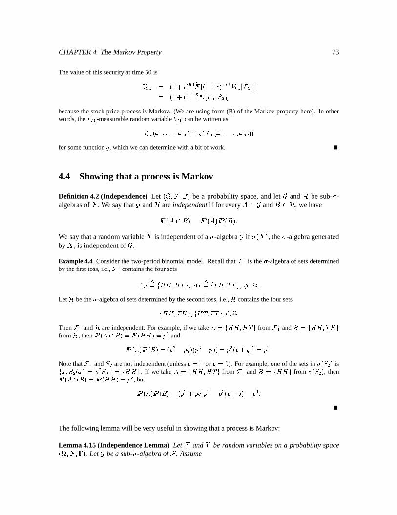
CHAPTER4. TheMarkov Property 73
Thevalueof thissecurityat time50 isá=Õ Ø Ð ÚAç| Õ Ý Õ Ø ÐÑ º ÚAç| Õ Ý i ÔAÔ á=Ô;Ô Ò ÏÃÕ Ø'Ð ÚAç| Õ Ý iµÙ Ô ÐÑ º á Ô;Ô Ò × Õ Ø Òbecausethestockpriceprocessis Markov. (We areusingform (B) of theMarkov propertyhere). In otherwords,the Ö Õ Ø -measurablerandomvariable
áVÕ Ø canbewrittenasá Õ Ø ÚÜÛ Ù Ò a$a$a Ò Û Õ Ø Ý ÐØ× Ú × Õ Ø ÚâÛ Ù Ò a@a$a Ò Û Õ Ø ÝAÝfor somefunction × , whichwecandeterminewith a bit of work.
4.4 Showing that a processis Mark ov
Definition 4.2(Independence)Let ø ì 2¤ ú be a probability space,andlet Ù and Ú be sub-Í -algebrasof ì . Wesaythat Ù and Ú areindependentif for every ÛPRÙ and ÜP\Ú , wehave øBÝRÜú ö ø ú2 øÜú/ûWe saythata randomvariable
óis independentof a Í -algebraÙ if Í8ø ó ú , the Í -algebragenerated
by
ó, is independentof Ù .
Example4.4 Considerthe two-periodbinomialmodel. RecallthatÏ Ù is the Þ -algebraof setsdetermined
by thefirst toss,i.e.,Ï Ù containsthefour setsßáàQâÐBã/ßß Ò ßàä Ò ßåæâÐçãà3ß Ò à8àä Ò.èEÒ?é a
Let ê bethe Þ -algebraof setsdeterminedby thesecondtoss,i.e., ê containsthefour setsã/ßß Ò à3ß ä Ò ã/ßà Ò à8àä ÒAè½ÒAé aThen
Ï Ù and ê areindependent.For example,if we takeß Ðmã/ßß Ò ßàä from
Ï Ù and ë+Ðìãßß Ò à3ß äfrom ê , then
Ñ í Ú ßæî ë Ý Ð Ñ í Ú ßß Ý Ð d o andÑ í Ú ß Ý Ñ í Ú ë Ý Ð Ú d o dhn Ý>Ú d o dJn Ý Ð d o Ú d n Ý o Ð d o aNotethat
Ï Ù and × o arenot independent(unlessd Ð ç or d Ðm` ). For example,oneof thesetsin Þ Ú × o Ý isã Û 5× o ÚâÛ¡Ý ÐrÏ o × Ø äÐïãßßðä . If we takeß Ðïãßß Ò ßàä from
Ï Ù and ë²Ðãßß ä from Þ Ú × o Ý , thenÑ í Ú ß]î ë Ý Ð Ñ í Ú ßß Ý Ð d o , butÑ í Ú ß Ý Ñ í Ú ë Ý Ð Ú d o dJn Ý d o Ð dVñ Ú d n Ý Ð dVñ aThefollowing lemmawill bevery usefulin showing thataprocessis Markov:
Lemma 4.15(IndependenceLemma) Let
óand ò be randomvariableson a probability spaceø ì Y¤ ú . Let Ù bea sub-Í -algebra of ì . Assume
74 Î ó is independentof Ù ;Î ò is Ù -measurable.
Let óø° @ô ú bea functionof twovariables,anddefine ø ô ú ôö /Dó8ø ó @ô ú/ûThen / óø ó òú<õÙ? ö ¡øòú/ûRemark. In this lemmaandthe following discussion,capitallettersdenoterandomvariablesandlowercaselettersdenotenonrandomvariables.
Example4.5(Showingthe stockprice processis Mark ov) Consideran ö -periodbinomial model. Fix a
time anddefine âÐ × u>e½Ù×hu and ÷ âÐ Ï u . Then
Ð(Ï if Û u>e½Ù3Ðfß and Ð Ó if Û u>e½Ù§Ðà . Since
dependsonly onthe Ú ÈçÝ st toss,
is independentof ÷ . Define ø âÐO×hu , sothat ø is ÷ -measurable.Let Ó
beany functionandset ù Ú_ ÒAú Ý âÐzÓ Ú_ ú Ý . Then× Ú ú Ý âÐ Ñ º ù Ú Ò;ú Ý Ð Ñ º Ó Ú ú Ý Ð d Ó Ú Ï ú Ý n Ó Ú Ó7ú Ý aTheIndependenceLemmaassertsthatÑ º Ó Ú × u>e½Ù>Ý@Ò Ï u> Ð Ñ º Ó 0 × u>e½Ù×hu a × u 1 Ò Ï u$Ð Ñ º ù Ú Ò ø Ý$Ò ÷ Ð × Ú ø ÝÐ d Ó Ú Ï©×hu Ý) n Ó Ú Ó ×hu Ý aThisshowsthestockpriceis Markov. Indeed,if weconditionbothsidesof theabove equationon Þ Ú ×hu Ý andusethetowerpropertyon theleft andthefact thattheright handsideis Þ Ú ×hu Ý -measurable,weobtainÑ º Ó Ú × u>e½ÙÝ@Ò × u$ Ð d Ó Ú Ï_× ukÝ~ n Ó Ú Ó × ubÝ aThus
Ñ º Ó Ú × u>e½ÙÝ@Ò Ï u> andÑ º Ó Ú × u>e½Ù°Ý$Ò u> areequalandform (b) of theMarkov propertyis proved.
Not only have we shown that the stockprice processis Markov, but we have alsoobtaineda formula forÑ º Ó Ú × u5e½Ù>Ý@Ò Ï u$ asa functionof × u . This is a specialcaseof Remark4.1.
4.5 Application to Exotic Options
Consideran -periodbinomialmodel.Definetherunningmaximumof thestockpriceto beThýôöüûý=þëYÿ " ÿµý ñ " ûConsidera simpleEuropeanderivativesecuritywith payoff at time of vø)ñ? TW©ú .Examples:
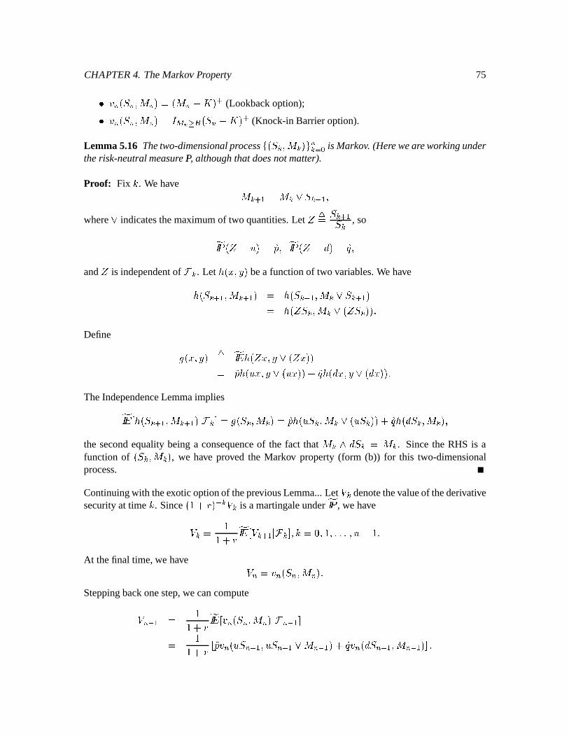
CHAPTER4. TheMarkov Property 75Î Eø)ñ? TC©ú ö øTCðÈú 9 (Lookbackoption);Î Eø)ñ? TC©ú ö ¦ø)ñ?ðÈú 9 (Knock-inBarrieroption).
Lemma 5.16 Thetwo-dimensionalprocess3¨ø)ñXý Thý7ú$6 ý & î is Markov. (Hereweareworkingundertherisk-neutral measure IP, althoughthatdoesnotmatter).
Proof: Fix E . We have Thý@9ë ö TOýBñXý$9ë where indicatesthemaximumof two quantities.Let d ôö ñ ý$9XëñXý , so
Ñø)d ö µú ö íø)d ö ú ö and d is independentof ìý . Let ¨ø° $ô ú bea functionof two variables.We have¨ø)ñXý$9ë Thý@9ëú ö ¨ø)ñXý$9ë Thý BñXý$9ëúö ¨ø)d ñXý TOýOø)d ñXý7ú#ú/ûDefine ø° @ô ú ôö /^¨ø)d¦° @ô ø)dðµú>úö ¨¡ø)° $ô ø°½ú>úE÷ ¨¡ø ° @ô ø °µú#ú/ûTheIndependenceLemmaimplies / ¨ø)ñ ý$9Xë T ý$9ë ú< ì ý ö ø)ñ ý T ý ú ö ¨øµñ ý T ý øµñ ý ú>úE÷ ¨¡ø ñ ý T ý ú the secondequalitybeinga consequenceof the fact that T ý ñ ý ö T ý . Sincethe RHS is afunction of ø)ñý Thý/ú , we have proved the Markov property(form (b)) for this two-dimensionalprocess.
Continuingwith theexotic optionof thepreviousLemma...Let êEý denotethevalueof thederivativesecurityat time E . Since ø5ù8÷fòbú 4 ý êý is amartingaleunder , we haveêEý ö ùù3÷ò / êEý$9ëZ< ìý5 E ö ù ûû/û íðùûAt thefinal time,we have ê) ö Xø)ñ? TW!úûSteppingbackonestep,wecancomputeê) 4 ë ö ùù÷(ò / vøNñ? TW©ú< ìS 4 ë;ö ùù÷(ò øµñ 4 ë ½ñ 4 ë \T 4 ë úX÷ ø ñ 4 ë T 4 ë ú©û
76
This leadsusto define v 4 ëø° $ô ú ôö ùù8÷fò vø)° ° ô úE÷ vø ° $ô úsothat ê) 4 ë ö 4 ë!ø)ñ? 4 ë TW 4 ë°úûThegeneralalgorithmisbý©ø° @ô ú ö ùù?÷fò ¬ bý$9ë!ø)° )° ô ú÷ bý$9ëkø ° @ô ú ¯Jandthe valueof the option at time E is bý©øNñXý TOýú . Sincethis is a simpleEuropeanoption, thehedgingportfolio is givenby theusualformula,which in thiscaseisïý ö bý$9Xëøµñý ø½ñXý7úRThý7ú§ðCký$9ë!ø ñXý TOýúøð ú>ñ ý
Chapter 5
StoppingTimesand American Options
5.1 American Pricing
Let us first review the Europeanpricing formula in a Mark ov model. Considerthe Binomialmodelwith periods.Let ê) ö ¡ø)ñ?_ú bethepayoff of a derivative security. Defineby backwardrecursion: Eø°µú ö ø°½úbý_ø°µú ö ùù3÷ò ký$9ë!ø)°µúE÷ bý$9Xëkø °½ú9ûThen ý ø)ñ ý ú is thevalueof theoptionat time E , andthehedgingportfolio is givenbyï ý ö ý$9ë øµñ ý ú8ðz ý$9ë ø ñ ý úøð ú>ñXý E ö ù X û7û/û íð(ùûNow consideran Americanoption. Again a function is specified. In any period E , the holderof the derivative securitycan“exercise”andreceive payment ø)ñý/ú . Thus,the hedgingportfolioshouldcreatea wealthprocesswhich satisfiesó ý ø)ñý/ú ;N E almostsurely.
This is becausethevalueof thederivativesecurityat time E is at least ¡ø)ñXý/ú , andthewealthprocessvalueat thattime mustequalthevalueof thederivativesecurity.
American algorithm.
Eø°µú ö ø°½úbý_ø°µú ö ûý7þ Þ ùù3÷fò ø bý$9Xëkø°µú÷ bý$9ë!ø °µú>ú ¡ø°µú Then bý©ø)ñý7ú is thevalueof theoptionat time E .
77
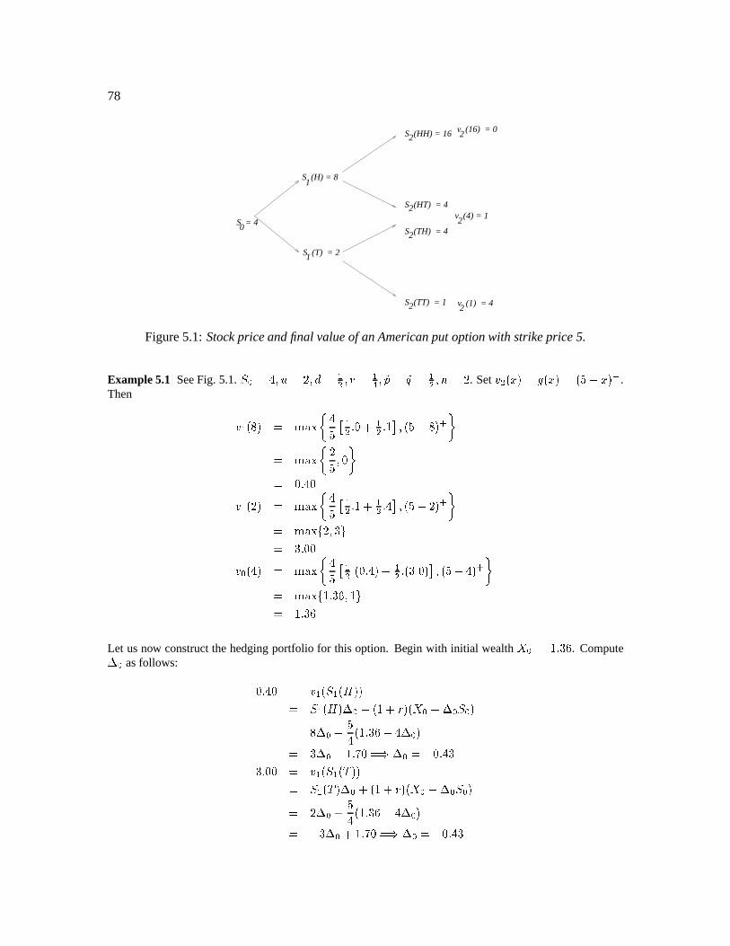
78
v (16) = 02
S = 40
S (H) = 8
S (T) = 2
S (HH) = 16
S (TT) = 1
S (HT) = 4
S (TH) = 4
1
1
2
2
2
2
v (4) = 1
v (1) = 4
2
2
Figure5.1: Stock priceandfinal valueof anAmericanput optionwith strikeprice5.
Example5.1 SeeFig. 5.1. ×Ø3Ð æ Ò Ï¦Ð ¹Ò9Ó Ð Ùo Ò5Õ Ð Ù Òvcd Ð cn Ð Ùo Ò öÐ ¹ . Set o Ú__Ý Ð]× Ú__Ý Ð Ú Ô ã\©Ý e .Then Ù Ú_Ý Ð pDr>s3Þ æÔ Ùo a` Ùo a ç Ò Ú Ô ã\7Ý e Ð pDr>s Þ ¹ Ô Ò ` Ð `ba æ ` Ù/Ú ¹ Ý Ð pDr>s Þ æ Ô Ùo a ç| Ùo a æ Ò Ú Ô ã ¹ Ý e Ð pDr>sVã ¹Ò w7äÐ wba `v` ØÚ&æbÝ Ð pDr>s3Þ æÔ Ùo a Ú `ba æbÝJ Ùo a Ú wVa` Ý Ò Ú Ô ãÑæbÝ e Ð pDr>sVã ç aw å Ò ç äÐ ç a w åLet usnow constructthehedgingportfolio for this option. Begin with initial wealth
Ø Ð ç aw å . Compute
Ø asfollows: `ba æ ` Ð ÙÚ × ÙÚ ß ÝAÝÐ × ÙÚ ß Ý ØÉÚAç| Õ Ý#Ú Øã Ø × ØÝÐ Ø? Ôæ ÚAç a w å?ãÑæ Ø>ÝÐ w Ø hç a `?Ð Ø8Ð ã `ba æ wwba `v` Ð ÙÚ × ÙÚ à ÝAÝÐ × ÙÚ à Ý Ø|ÚAç| Õ Ý>Ú Øã Ø × ØÝÐ ¹ Ø? Ôæ ÚAç a w å?ãÑæ Ø>ÝÐ ã w Ø?hç a `?Ð Ø Ð ã `ba æ w
CHAPTER5. StoppingTimesandAmericanOptions 79
Using
ØÐ ã `Va æ w resultsin Ù Ú ß Ý ÐzÙ Ú ×½Ù Ú ß ÝÝ Ðz`ba æ ` Ò Ù Ú à Ý ÐxÙ Ú ×½Ù Ú à ÝAÝ ÐxwVa``Now let uscompute
Ù (Recallthat × ÙÚ à Ý Ð ¹ ):ç Ð o Ú&æbÝÐ × o Ú à3ß Ý ÙÚ à ÝÚç| Õ Ý>Ú Ù/Ú à ÝEã ÙÚ à Ý × Ù7Ú à ÝÝÐ æ ÙÚ à Ý~ Ôæ Ú w ã ¹ ÙÚ à ÝÝÐ ç aÔ Ù Ú à Ý) wVa Ô3Ð Ù Ú à Ý Ð ãZç a wæ Ð o ÚAçÝÐ × o Ú à8à Ý Ù Ú à Ý)Úç Õ Ý#Ú Ù Ú à ÝEã Ù Ú à Ý ×½Ù Ú à ÝAÝÐ ÙÚ à Ý Ôæ Ú w ã ¹ ÙÚ à ÝAÝÐ ãZç a Ô Ù Ú à Ý wVa ÔÐ Ù Ú à Ý Ð ã `Va çåWe getdifferentanswersfor
ÙÚ à Ý ! If wehad ÙÚ à Ý Ð ¹ , thevalueof theEuropeanput,wewouldhaveç Ð ç aÔ Ù Ú à Ý) ¹ a ÔÐ Ù Ú à Ý Ð ãZç Òæ Ð ãZç aÔ ÙÚ à Ý~ ¹ aÔ?Ð ÙÚ à Ý Ð ãZç Ò
5.2 Valueof Portf olio Hedgingan American Optionó ý$9Xë ö ïýbñXý@9ë¡÷ø5ù?÷òkúø ó ýZð ýZðïýbñXýúö ø5ù3÷òbú ó ý?÷ïýø)ñXý$9Xë3ðfø°ù3÷òbú>ñXý7úð+ø5ù8÷fòbúSýHere, ý is theamount“consumed”at time E .Î Thediscountedvalueof theportfolio is asupermartingale.Î Thevaluesatisfies
ó ý ø)ñý/ú E ö ù ûû/û .Î Thevalueprocessis thesmallestprocesswith theseproperties.
Whendoyouconsume?If /Ñø#ø5ù3÷òbú 4?8 ý$9ëA: bý$9ëkø)ñXý$9Xëúv< ìý$¯ø5ù?÷òkú 4 ý bý©øNñXý7ú or, equivalently, /Ñø ùù?÷ò ý$9ë ø)ñ ý$9Xë úv< ì ý Q ý ø)ñ ý ú
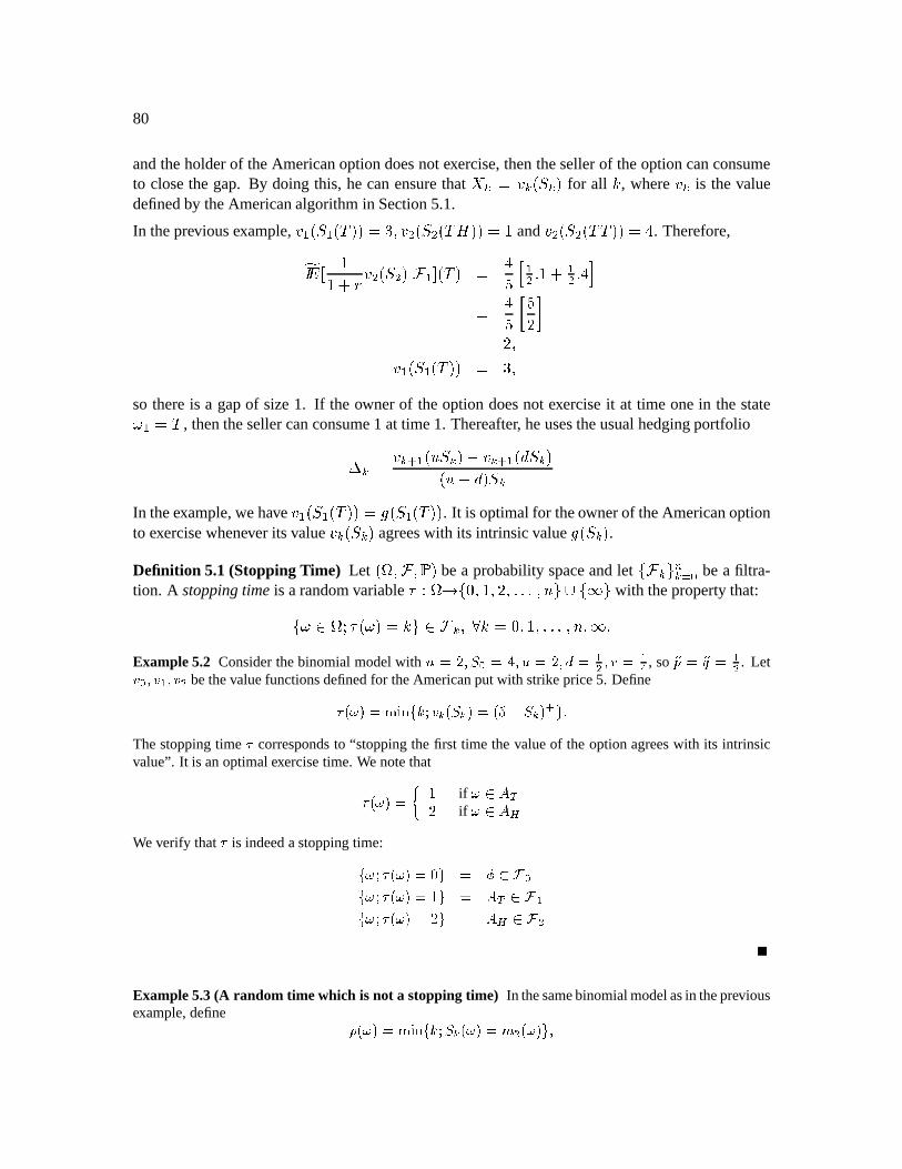
80
andtheholderof theAmericanoptiondoesnot exercise,thenthesellerof theoptioncanconsumeto closethe gap. By doing this, hecanensurethat
ó ý ö ý ø)ñ ý ú for all E , where ý is the valuedefinedby theAmericanalgorithmin Section5.1.
In thepreviousexample,ëkøNñëøÿéSú>ú ö 7bø)ñ|bøüéSèÈú>ú ö ù and 7kø)ñÉøüéZéSú>ú ö . Therefore, / ùù8÷fò 7bø)ñ|/ú< ìë;°øüéSú ö ! ² ë û&ù8÷ ë ûV¶ö ! ¬ !X ¯ö X ë ø)ñ ë øüéSú>ú ö so thereis a gapof size1. If the ownerof theoption doesnot exerciseit at time onein the stateþZë ö é , thenthesellercanconsume1 at time1. Thereafter, heusestheusualhedgingportfolioïý ö ký$9ë!ø½ñXý7úðxký$9ëkø ñXý7úøð ú>ñýIn theexample,wehave ëkø)ñë7øüéSú>ú ö ¡ø)ñë/øüéSú>ú . It is optimalfor theownerof theAmericanoptionto exercisewhenever its value ý ø)ñ ý ú agreeswith its intrinsicvalue øNñ ý ú .Definition 5.1(StoppingTime) Let ø ì 2¤ ú bea probabilityspaceandlet 3ìý=6 ý & î bea filtra-tion. A stoppingtime is a randomvariable"BeVK¢m3, ù X û/û/û É6 #]3,©m6 with thepropertythat:3þçP£U$"Xøþ3ú ö E)6DPBìý !N E ö ù û7û/û ©+ûExample5.2 Considerthebinomialmodelwith öBÐ ¹Ò × Ø Ð æ Ò ÏÐ ¹Ò5Ó Ð Ùo Ò5Õ Ð Ù , so cd Ð cn Ð Ùo . Let Ø Ò Ù Ò o bethevaluefunctionsdefinedfor theAmericanputwith strikeprice5. Define% ÚÜÛ¡Ý Ð]p'&)(Jã>~;$u Ú ×hu Ý Ð Ú Ô ã ×hu Ý e ä,aThestoppingtime % correspondsto “stoppingthe first time the valueof the optionagreeswith its intrinsicvalue”. It is anoptimalexercisetime. We notethat% ÚÜÛ¡Ý Ð Þ ç if Û* ßå¹ if Û* ßàWe verify that % is indeedastoppingtime:ã Û % ÚÜÛXÝ Ðz`=ä Ð è * Ï Øã Û % ÚÜÛXÝ Ð ç ä Ð ß å * Ï Ùã Û % ÚÜÛXÝ Ð ¹ ä Ð ß à * Ï£oExample5.3(A random time which is not a stopping time) In thesamebinomialmodelasin thepreviousexample,define + ÚâÛÝ ÐWp&)(Vã>~9× uÚâÛ¡Ý Ð-, o ÚâÛ¡Ý ä Ò
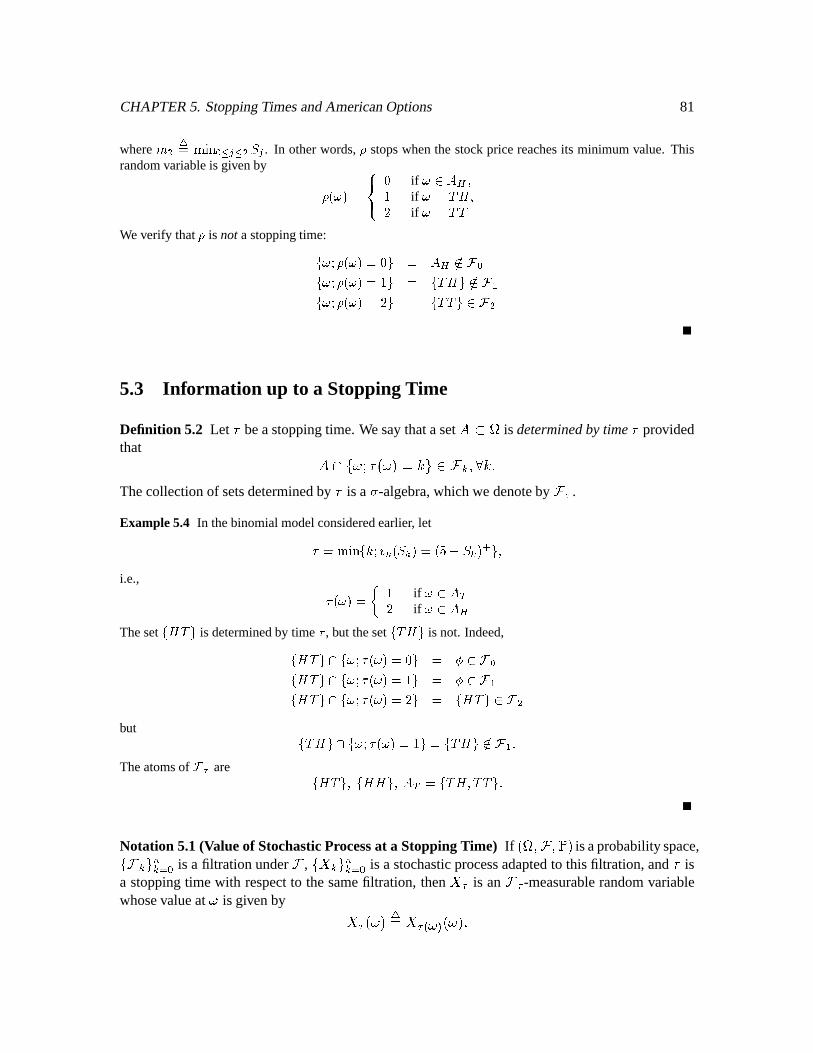
CHAPTER5. StoppingTimesandAmericanOptions 81
where , o âÐp&)( ØYt/.>t o × . . In otherwords,+
stopswhenthe stockpricereachesits minimumvalue. Thisrandomvariableis givenby + ÚÜÛ8Ý Ð102 3 ` if Û* ß à Òç if Û Ðà3ß Ò¹ if Û Ðà8àWe verify that
+is not a stoppingtime:ã Û + ÚÜÛ¡Ý Ðx`7ä Ð ß à y* Ï Øã Û + ÚÜÛ¡Ý Ð ç ä Ð ãà3ß äÃy* Ï Ùã Û + ÚÜÛ¡Ý Ð ¹ ä Ð ãà8àä * Ï£o
5.3 Information up to a StoppingTime
Definition 5.2 Let " beastoppingtime. Wesaythataset Ám is determinedby time " providedthat xÝ]3/þ¦U"øaþ§ú ö E)6^PBì ý ;N EEûThecollectionof setsdeterminedby " is a Í -algebra,whichwe denoteby ì4 .Example5.4 In thebinomialmodelconsideredearlier, let% ÐWp&)(Vã>~; uÚ × ukÝ Ð Ú Ô ã × ukÝ e ä Òi.e., % ÚÜÛ¡Ý Ð Þ ç if Û* ß å¹ if Û* ß àTheset ã/ßàä is determinedby time % , but theset ãà3ß ä is not. Indeed,ãßàä î ã Û % ÚâÛ¡Ý Ðx`7ä Ð è * Ï Øãßàä î ã Û % ÚâÛ¡Ý Ð ç ä Ð è * Ï Ùãßàä î ã Û % ÚâÛ¡Ý Ð ¹ ä Ð ãßàä * ÏÎobut ãà3ßðä î ã Û % ÚÜÛ¡Ý Ð ç ä3ÐBãà3ß ä£y* Ï Ù aTheatomsof
Ï5are ãßàä Ò ã/ßß ä Ò ß å ÐBãà3ß Ò à8àä,a
Notation 5.1(Valueof StochasticProcessat a StoppingTime) If ø ì Y¤ ú isaprobabilityspace,37ìý76 ý & î is a filtration underì , 3 ó ý76 ý & î is a stochasticprocessadaptedto thisfiltration, and " isa stoppingtime with respectto thesamefiltration, then
ó 4 is an ì 4 -measurablerandomvariablewhosevalueat þ is givenby
ó 4øþ<úôö ó 4 8 þ : øþ<ú/û
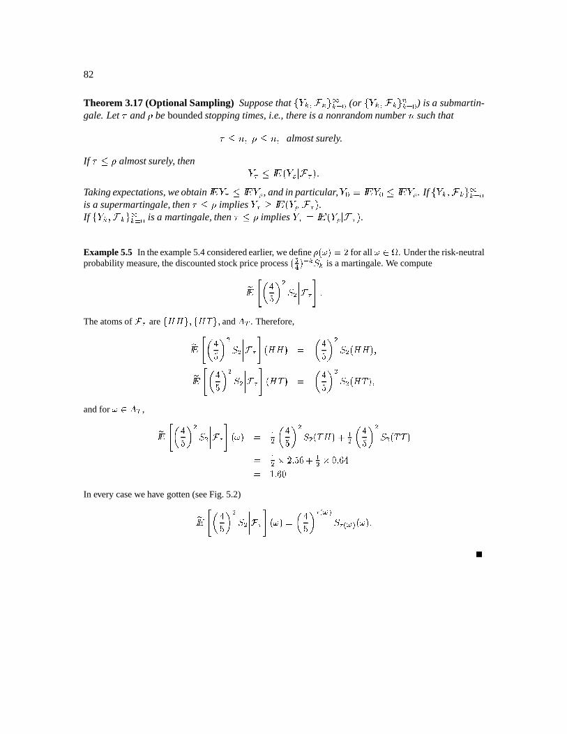
82
Theorem 3.17(Optional Sampling) Supposethat 3òý ìxýb676ý & î (or 3òEý ìxý=6 ý & î ) is a submartin-gale. Let " and 8 beboundedstoppingtimes,i.e., there is a nonrandomnumber such that" 8 almostsurely.
If " 8 almostsurely, then ò94 /Bøò;:V< ì<4bú/ûTakingexpectations,weobtain / ò 4 / ò : , andin particular, ò î ö / ò î / ò : . If 3ò ý ì ý 6/6ý & îis a supermartingale, then " 8 implies ò=4>Q /Bøò:V< ì4ú .If 3òý ìý76 6ý & î is a martingale,then " 8 implies ò94 ö /Bøò:,< ì4ú .Example5.5 In theexample5.4consideredearlier, wedefine
+ ÚÜÛ¡Ý Ð ¹ for all Û* é . Undertherisk-neutralprobabilitymeasure,thediscountedstockpriceprocessÚ Õ Ý ihu × u is a martingale.We computeÐÑ º@? 0 æ Ô 1 o × o ®®®® Ï5A aTheatomsof
Ï5are ã/ßß ä Ò ã/ßàä Ò and
ß å. Therefore,ÐÑ º ? 0 æ Ô 1 o × o ®®®® Ï5 A Ú ßß Ý Ð 0 æ Ô 1 o × o Ú ßß Ý ÒÐÑ º ? 0 æ Ô 1 o × o ®®®® Ï 5 A Ú ßà Ý Ð 0 æ Ô 1 o × o Ú ßà Ý Ò
andfor ÛB* ß å , ÐÑ º ? 0 æ Ô 1 o × o ®®®® Ï5 A ÚâÛÝ Ð Ùo 0 æ Ô 1 o × o Ú à3ß Ý) Ùo 0 æ Ô 1 o × o Ú à8à ÝÐ Ùo ¹ aÔ å Ùo S`ba å/æÐ ç a å `In every casewehave gotten(seeFig. 5.2)ÐÑ ºC? 0 æ Ô 1 o × o ®®®® Ï 5 A ÚÜÛÝ Ð 0 æ Ô 1 5D ÛFE × 5D ÛGE ÚÜÛ¡Ý a
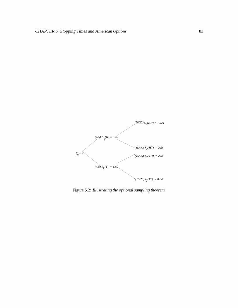
CHAPTER5. StoppingTimesandAmericanOptions 83
S = 40
1
2
2
2
2
S (HH) = 10.24
S (HT) = 2.56
S (TH) = 2.56
S (TT) = 0.64
1S (T) = 1.60(4/5)
S (H) = 6.40(4/5)
(16/25)
(16/25)
(16/25)
(16/25)
Figure5.2: Illustratingtheoptionalsamplingtheorem.

84
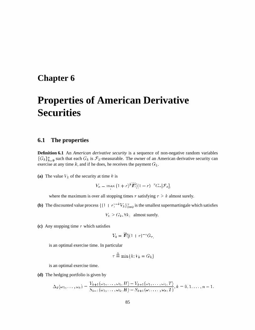
Chapter 6
Propertiesof American DerivativeSecurities
6.1 The properties
Definition 6.1 An Americanderivativesecurity is a sequenceof non-negative randomvariables3IHý76 ý & î suchthateachHý is ìý -measurable.Theownerof anAmericanderivative securitycanexerciseatany time E , andif hedoes,hereceivesthepaymentHý .(a) Thevalue êEý of thesecurityat time E isêEý öÛûý7þ4 ø°ù3÷òbú ý / ø5ù3÷òbú$4 4 H4< ìý$
wherethemaximumis over all stoppingtimes " satisfying"JQE almostsurely.
(b) Thediscountedvalueprocess3¨ø5ù8÷fòbú 4 ý êý=6 ý & î is thesmallestsupermartingalewhichsatisfiesêEýKHý 'N E almostsurely.
(c) Any stoppingtime " whichsatisfies ê½î ö / ø5ù8÷fòbú 4 4 H'4>is anoptimalexercisetime. In particular"BôöÛû ½´¾)3,E?UêEý ö Hý76is anoptimalexercisetime.
(d) Thehedgingportfolio is givenbyïý©øþ3ë û7ûû þýú ö ê ý$9ë øþ ë ûû7û þ ý èÈúXðê ý@9ë øþ ë û7ûû þ ý éSúñXý$9Xëøþ3ë ûû7û þý èÈúXðñXý$9ë!øþ3ë ûû7û þý éSú E ö ù ûû7û íðùû85
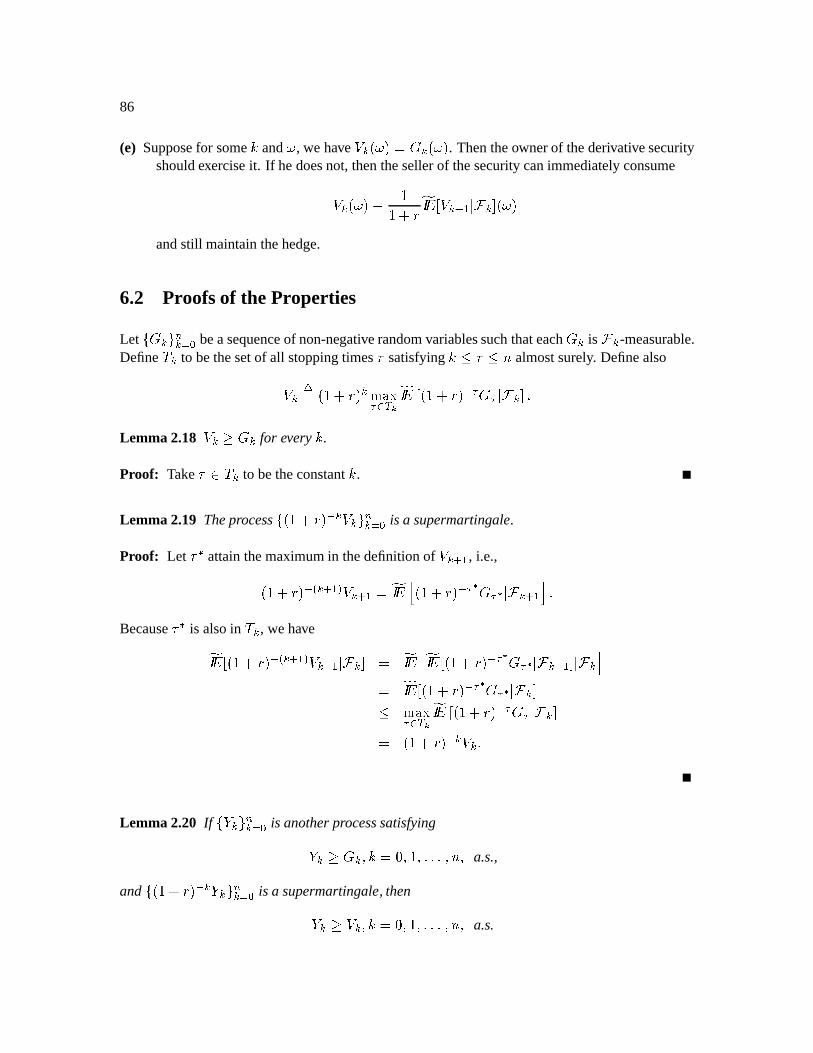
86
(e) Supposefor someE and þ , we have êEý©øþ3ú ö Hxý©øaþ§ú . Thentheownerof thederivativesecurityshouldexerciseit. If hedoesnot, thenthesellerof thesecuritycanimmediatelyconsumeê ý øaþ§ú8ð ùù8÷fò / ê ý$9ë < ì ý °øaþ§úandstill maintainthehedge.
6.2 Proofsof the Properties
Let 3LHxý76 ý & î beasequenceof non-negativerandomvariablessuchthateachHxý is ìý -measurable.Define éXý to bethesetof all stoppingtimes " satisfyingE " almostsurely. Definealsoê ýôö ø°ù÷(òbú ý ûý7þ4/M - Ä / ø5ù3÷òbú$4 4 H 4 < ì ý ©ûLemma 2.18 êEýKHý for every E .Proof: Take "¥PBéXý to betheconstantE .Lemma 2.19 Theprocess3¨ø5ù?÷òkú54 ý ê ý 6 ý & î is a supermartingale.
Proof: Let "N attainthemaximumin thedefinitionof êEý@9ë , i.e.,ø5ù3÷òbú 4?8 ý@9ëA: êý$9ë ö /²)ø5ù3÷òbú 4 4/O H4 O < ìý@9ë2¶8ûBecause"N is alsoin éXý , wehave / ø°ù÷(òbú$4?8 ý$9ëA: êEý$9Xë< ìýZ ö /·² / ø5ù8÷òbú$4 4 O H4 O < ìý@9ë;'< ìýZ¶ö / ø5ù8÷fòbú$4 4 O H 4 O < ì ý ûý=þ4/M - Ä / ø5ù8÷òbú 4 4 H4k< ìý5ö ø5ù8÷(òkú 4 ý êEýûLemma 2.20 If 3òý=6 ý & î is anotherprocesssatisfyingòý<KHý E ö ù û7û/û a.s.,
and 3¨ø5ù8÷òbú$4 ý òEýb6 ý & î is a supermartingale, thenòEý<fêEý E ö ù ûû7û a.s.
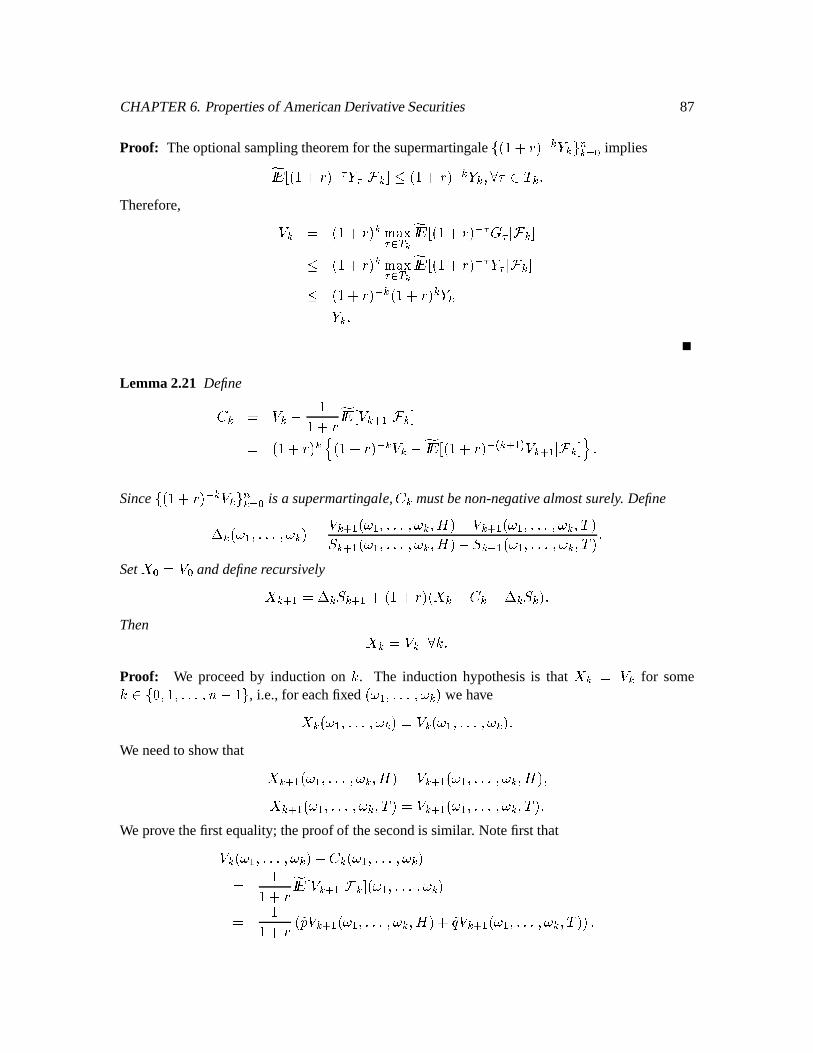
CHAPTER6. Propertiesof AmericanDerivativeSecurities 87
Proof: Theoptionalsamplingtheoremfor thesupermartingale3¨ø5ù3÷òbú$4 ý òEýb6 ý & î implies / ø°ù3÷òbú 4 4 ò94< ìýZ ø5ù8÷(òkú 4 ý òý ;N " PBéXýûTherefore, êEý ö ø5ù8÷òkú ý ûý=þ4/M - Ä / ø5ù8÷òbú 4 4 H4~< ìý$ ø5ù8÷òkú ý ûý=þ4/M - Ä / ø5ù8÷òbú 4 4 ò94< ìý> ø5ù8÷òkú 4 ý ø5ù8÷(òkú ý òýö òýûLemma 2.21 DefineSý ö êEýZð ùù3÷(ò / êEý$9Xë,< ìxýZö ø5ù3÷òbú ýGP ø5ù3÷òbú 4 ý êEýZðW / ø5ù8÷fòbú 4?8 ý$9ëA: êEý$9ëZ< ìýZRQ¦ûSince3¨ø5ù8÷(òkú 4 ý êEý76 ý & î is a supermartingale, Sý mustbenon-negativealmostsurely. Defineïý©øaþ3ë ûû7û þ8ý7ú ö êEý@9ëkøþ?ë û7û7û þý èÈúXðêEý$9ëkøþ3ë ûû7û þý éSúñXý$9ë!øþ?ë û7û7û þý èÈúXðñý@9ë!øaþ3ë û7ûû þ8ý é ú ûSet
ó î ö ê î anddefinerecursivelyó ý$9ë ö ïýñXý@9ë8÷ø5ù3÷òbú7ø ó ýðSSýZðïý7ñXýú/ûThen
ó ý ö êEý N EEûProof: We proceedby induction on E . The induction hypothesisis that
ó ý ö êEý for someE\P]37 ù û/û7û íðù76 , i.e., for eachfixed øþ?ë û7û7û þý/ú we haveó ý øþ ë û7û7û þ ý ú ö ê ý øþ ë û7û7û þ ý úûWe needto show that ó ý$9Xë øaþ ë û7ûû þ ý èÈú ö ê ý@9ë øþ ë û7û7û þ ý èÈú ó ý$9ëkøþ3ë ûû7û þý éSú ö êEý@9ë7øþ3ë û7û7û þý éSú/ûWe prove thefirst equality;theproofof thesecondis similar. Notefirst thatê ý øþ ë û7ûû þ ý ú8ð ý øaþ ë ûû7û þ ý úö ùù8÷(ò / êEý$9Xë,< ìý5°øþ3ë ûû7û þý/úö ùù8÷(ò ø ê ý$9ë øþ ë ûû7û þ ý èÈúµ÷ ê ý@9ë øþ ë û7ûû þ ý éSú>ú½û
88
Since øþ3ë û7û7û þý/ú will be fixed for the restof the proof, we will suppressthesesymbols. Forexample,thelastequationcanbewrittensimplyasêýðSý ö ùù3÷ò ø êEý@9ëkø)èÈúE÷ êEý@9ëkøüéSú#úµûWe compute ó ý$9ëkø)èÈú ö ïýbñXý@9ëkø)èÈúE÷ø5ù3÷òbú7ø ó ýðSýðïý7ñýkúö êEý$9ëkø)èÈú¡ðêEý$9ëkøüéSúñXý@9ëø)èÈú¡ðñý@9ëkøüéSú øNñXý@9ëkø)èÈúðfø5ù3÷òbú>ñý7ú÷ø5ù3÷(òkúø)êEýðSý7úö êý$9ëkø)èÈúðOêEý@9ëkøüé úøð ú#ñXý ø½ñXýZð+ø5ù8÷fòbú>ñXý/ú÷ êEý@9ëkø)èÈúE÷ êEý$9XëkøÿéSúö ø)êEý@9ëkø)èÈúðêEý@9ëkøüéSú#ú ÷ êEý@9ë7ø)èÈú÷ êý$9ëkøüéSúö êý$9ëkø)èÈú/û6.3 CompoundEuropeanDerivative Securities
In orderto derive theoptimalstoppingtime for anAmericanderivativesecurity, it will beusefultostudycompoundEuropeanderivativesecurities,which arealsointerestingin their own right.
A compoundEuropeanderivative securityconsistsof Ñ÷²ù differentsimpleEuropeanderivativesecurities(with the sameunderlyingstock)expiring at times ù û7û/û ; the securitythatexpiresat time À haspayoff " . Thusa compoundEuropeanderivativesecurityis specifiedby theprocess3I " 6 " & î , whereeach " is ì " -measurable,i.e., the process3L " 6 " & î is adaptedto the filtration37ìý76 ý & î .Hedging a short position (onepayment). Hereis how we canhedgea shortpositionin the À ’ thEuropeanderivativesecurity. Thevalueof EuropeanderivativesecurityÀ at time E is givenbyê 8 " :ý ö ø°ù3÷òbú ý / ø5ù8÷fòbú 4 " " < ìý$ E ö ûû7û À andthehedgingportfolio for thatsecurityis givenbyï 8 " :ý øþ3ë û7ûû þýú ö ê 8 " :ý$9Xë øaþ3ë ûû7û þ8ý èÈúðê 8 " :ý@9ë øþ?ë û7ûû þý éSúñ 8 " :ý$9Xë øaþ3ë ûû7û þ8ý èÈúðñ 8 " :ý$9ë øþ3ë ûû7û þý éSú E ö û7û7û ÀðùûThus,startingwith wealth ê 8 " :î , andusingthe portfolio ø)ï 8 " :î ûû7û ï 8 " :" 4 ë ú , we canensurethat attime À wehave wealth " .Hedging a short position (all payments). Superposethe hedgesfor the individual payments.Inotherwords,startwith wealth ê½î öUT " & î ê 8 " :î . At eachtime E P]3, ù ûû/û íðù76 , first makethepaymentSý andthenusetheportfolioïý ö ïý 8 ý$9Xë;: ÷fïý 8 ý@9?2: ÷+û7û7û÷fïý 8 7:
CHAPTER6. Propertiesof AmericanDerivativeSecurities 89
correspondingto all futurepayments.At the final time , aftermakingthefinal payment+ , wewill have exactly zerowealth.
Supposeyou own a compoundEuropeanderivativesecurity3I " 6 " & î . Compute
ê î ö V" & î ê 8 " :î ö /XWY V" & î ø5ù8÷fòbú 4 " "Z[andthehedgingportfolio is 3kïý=6 4 ëý & î . Youcanborrow ê½î andconsumeit immediately. This leavesyou with wealth \^]_a`cb=] . In eachperiod d , receivethepaymentegf andthenusetheportfolio`ch f . At thefinal time , afterreceiving thelastpaymenteci , yourwealthwill reachzero,i.e.,youwill no longerhave a debt.
6.4 Optimal Exerciseof American DerivativeSecurity
In thissectionwederivetheoptimalexercisetimefor theownerof anAmericanderivativesecurity.Let jLk f/l i f$m=] be an Americanderivative security. Let n be the stoppingtime the ownerplanstouse.(Weassumethateachk f is non-negative,sowemayassumewithout lossof generalitythattheownerstopsat expiration– time – if notbefore).Usingthestoppingtime n , in periodo theownerwill receive thepayment eqpr_tsvuw m pyx kzp7In otherwords,oncehechoosesa stoppingtime, theownerhaseffectively convertedtheAmericanderivativesecurityinto a compoundEuropeanderivativesecurity, whosevalueis
b^| wI] _ s ~X ip m=]FyF/ p ep_ s ~ ip m=] yF/ p svuw m pyx kp _ s ~ GK/ w k wv The ownerof the Americanderivative securitycanborrow this amountof money immediately, ifhechooses,andinvestin themarketsoasto exaclty payoff his debtasthepaymentsjIep l ip m=] are
received.Thus,his optimalbehavior is to useastoppingtime n whichmaximizesb<| wI] .
Lemma 4.22 b| wI] is maximizedby thestoppingtimen_t<j/d$b f _ k f/l Proof: Recallthedefinitionb ]_U>/w//I s ~ yFK/ w k w _t>/w/7L b | wI]
90
Let n beastoppingtimewhichmaximizesb | wI] , i.e., b ] _Ûs ~ yF/ wI¡ k w ¡)¢ Becausej y K/ f b f/l i fm=]is a supermartingale,wehave from theoptionalsamplingtheoremandtheinequality b f£ k f , thefollowing: b ] £ s ~ K/ w ¡ b w ¡¥¤ ¦ ] ¢_ s ~ K/ wI¡ b w ¡ ¢£ s ~ K/ w ¡ k w ¡§¢_ b=]/Therefore, b ] _Ûs ~ G/ w ¡ b w ¡¨¢ _Ûs ~ yF/ w ¡ k w ¡)¢G©and b w ¡ _ k w ¡ª© a.s.
We have justshown thatif n attainsthemaximumin theformulab ] _t>w//I s ~ G/ w k wv © (4.1)
then b w ¡ _ k w ¡ © a.s.
But wehave defined n _t<j/d$b f _ k f/l ©andsowemusthave n « n ;« almostsurely. Theoptionalsamplingtheoremimplies
K/ w/¬ k w ¬ _ yFK/ w/¬ b w ¬£ s ~ K/ wI¡ b w ¡¥¤ ¦ w ¬ ¢_ s ~ K/ w ¡ k w ¡ ¤ ¦ w ¬ ¢ Takingexpectationsonbothsides,weobtain s ~ K/ w ¬ k w ¬ ¢ £ s ~® K/ wI¡ k w ¡¨¢ _tb ] It follows that n alsoattainsthemaximumin (4.1), andis thereforeanoptimalexercisetime fortheAmericanderivativesecurity.
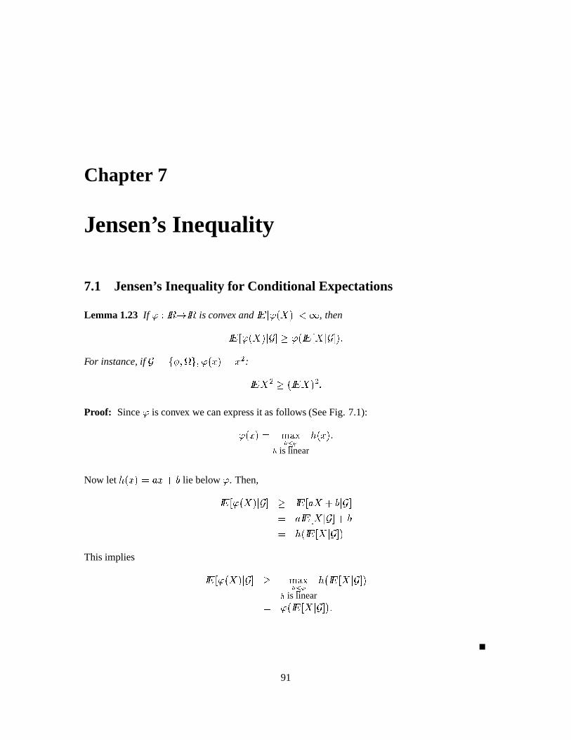
Chapter 7
Jensen’s Inequality
7.1 Jensen’s Inequality for Conditional Expectations
Lemma 1.23 If ¯he°s ±²s ± is convex and s ~ ¤ ¯ \ ¤L³´ , thens ~§¯ \ ¤¶µ £ ¯ s ~·\ ¤·µ For instance,if µ _@j/¸ ©¹ l © ¯ ¥º9 _ º=» : s ~'\ » £ s ~'\ » Proof: Since ¯ is convex wecanexpressit asfollows(SeeFig. 7.1):¯ ¥º9 _ >/¼¾½¿À
is linear Á ¥º9 Now let Á º9 _U º'Kà lie below ¯ . Then,s ~§¯ \ ¤¶µ £ s ~§ÂÄ\ Kà ¤·µ _ ÂÅs ~ƶ\ ¤¶µ KÃ_ Á s ~ƶ\ ¤¶µ This implies s ~§¯ \ ¤·µ £ >/¼¾½¿À is linear Á s ~·\ ¤·µ _ ¯ s ~·\ ¤·µ
91
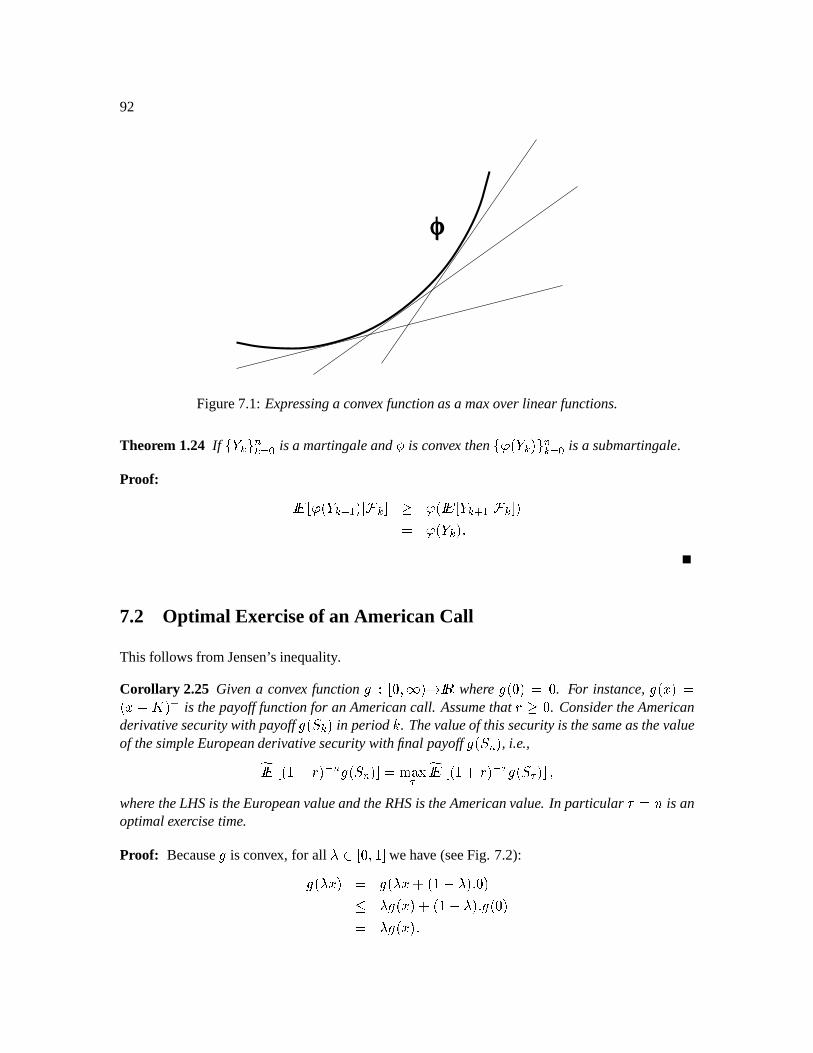
92
ϕ
Figure7.1: Expressinga convex functionasa maxoverlinear functions.
Theorem 1.24 If jIÇ fl i f$m=] is a martingaleand ¸ is convex then j7¯ Ç f l i f$m=] is a submartingale.
Proof: s ~§¯ Ç f$ÈÊÉ ¤ ¦ f £ ¯ s ~·Ç fÈÊÉ ¤ ¦ f _ ¯ Ç f 7.2 Optimal Exerciseof an American Call
This followsfrom Jensen’s inequality.
Corollary 2.25 Givena convex function Ë+er¨Ì ©$´ ²s ± where Ë Ì _ÍÌ . For instance,Ë ¥º9 _¥º `-Î È is thepayoff functionfor anAmericancall. Assumethat £ Ì . ConsidertheAmericanderivativesecuritywith payoff Ë ¥Ï f in period d . Thevalueof thissecurityis thesameasthevalueof thesimpleEuropeanderivativesecuritywith final payoff Ë Ï i , i.e., s ~ y K/ i Ë ¥Ï i _t^/w s ~ G7 w Ë Ï w ©where theLHSis theEuropeanvalueandtheRHSis theAmericanvalue. In particular n>_ is anoptimalexercisetime.
Proof: BecauseË is convex, for all ÐÒÑ§Ì © wehave (seeFig. 7.2):Ë Ð º9 _ Ë Ð ºt `Ð §Ì « ÐÅË ¥º=;ty `Ð Ë Ì _ ÐÅË ¥º=
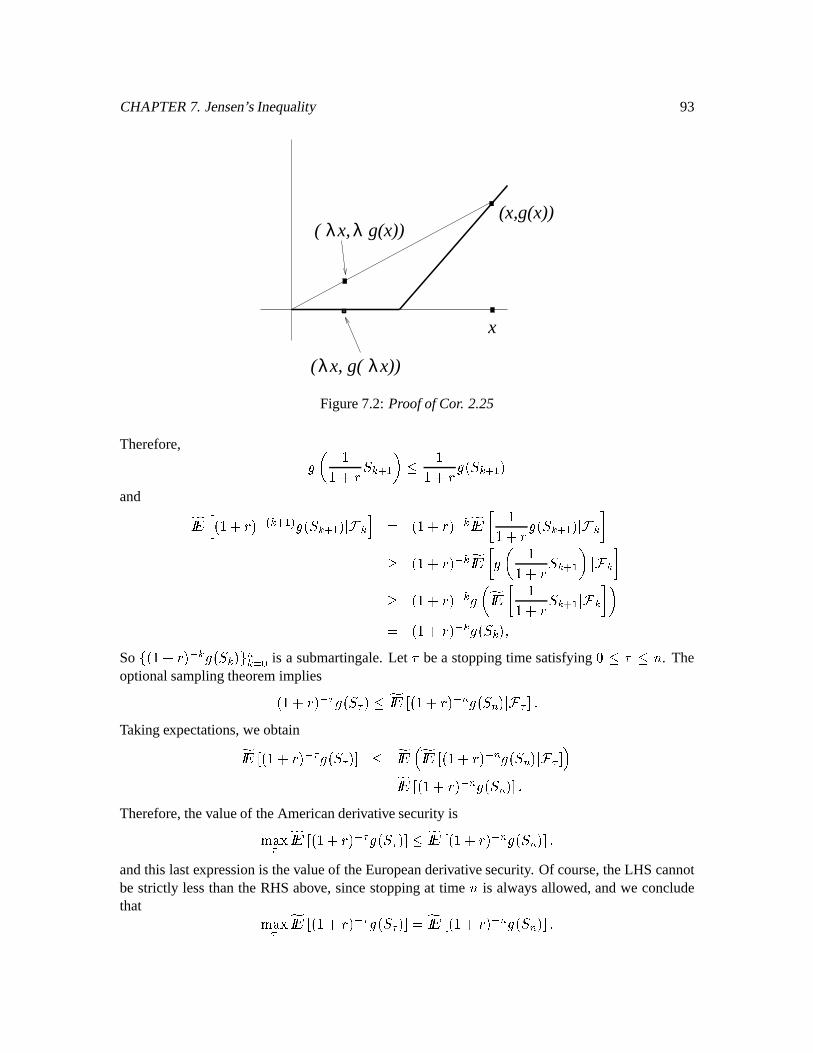
CHAPTER7. Jensen’sInequality 93
( x, g(x))λλ
( x, g( x))λ λ
(x,g(x))
x
Figure7.2: Proofof Cor. 2.25
Therefore, ËÔÓ Ï fÈÕÉÖ « K Ë Ï f$ÈÊÉ and s ~ K/ | f$ÈÊÉ Ë Ï f$ÈÊÉ ¤ ¦ f ¢ _ G/ f s ~®× K Ë Ï f$ÈÊÉ ¤ ¦ fØ£ G/ f s ~ × ËÔÓ F Ï f$ÈÊÉ Ö ¤ ¦ f Ø£ G/ f ËJÓV s ~ × F Ï f$ÈÊÉ ¤ ¦ f Ø Ö_ G/ f Ë ¥Ï f ©So j GK7 f Ë ¥Ï f l i f$m=] is a submartingale.Let n bea stoppingtime satisfying Ì « n « . TheoptionalsamplingtheoremimpliesyF/ w Ë ¥Ï w « s ~ G/ i Ë ¥Ï i ¤ ¦ wv Takingexpectations,weobtain s ~ K7¾ w Ë ¥Ï w « s ~CÙ2 s ~ G/ i Ë ¥Ï i ¤ ¦ wvªÚ_ s ~ G/ i Ë ¥Ï i Therefore,thevalueof theAmericanderivativesecurityis>/w s ~ G/ w Ë ¥Ï w « s ~ K/ i Ë ¥Ï i ©andthis lastexpressionis thevalueof theEuropeanderivativesecurity. Of course,theLHS cannotbestrictly lessthanthe RHSabove, sincestoppingat time Û is alwaysallowed,andwe concludethat >/w s ~ G/ w Ë ¥Ï w _Ûs ~ K/ i Ë ¥Ï i
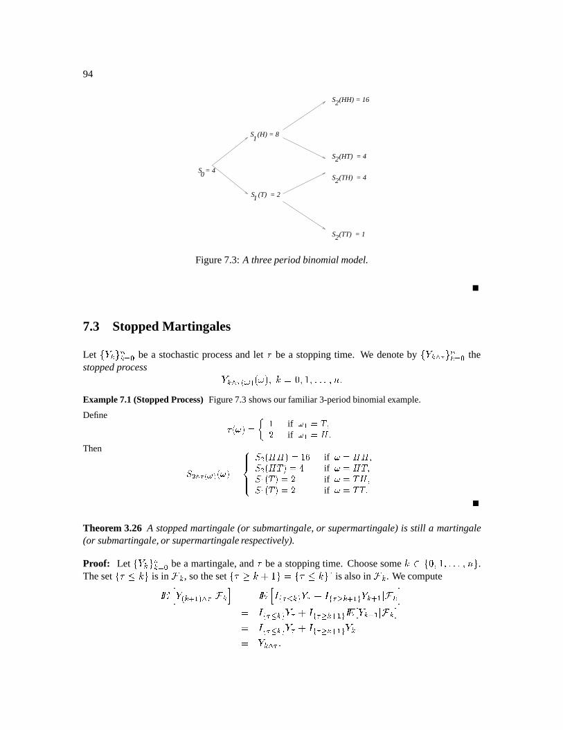
94
S = 40
S (H) = 8
S (T) = 2
S (HH) = 16
S (TT) = 1
S (HT) = 4
S (TH) = 4
1
1
2
2
2
2
Figure7.3: A threeperiodbinomialmodel.
7.3 StoppedMartingales
Let jLÇ f/l i f$m=] be a stochasticprocessandlet n be a stoppingtime. We denoteby jIÇ fÜ w l i fm=] thestoppedprocess Ç fÜ w |¨Ý Ý © d>_UÌ © © Iv © ÛÞExample7.1(StoppedProcess)Figure7.3showsour familiar 3-periodbinomialexample.
Define ßà)áGâ;ã äåif
áFæÞãSçGèéif
áFæÞãê>ëThen ìíî/ïð áFñ àòáFâã1óôôõ ôôö
ì í àªê>ê>âÕã å÷if
áÔã-ê^ê>èì í àªê<ç âÕãSøif
áÔã-êçFèì æ¾àùç âÕã éif
áÔãç ê^èì æ¾àùç âÕã éif
áÔãçGçGëTheorem 3.26 A stoppedmartingale(or submartingale,or supermartingale)is still a martingale(or submartingale,or supermartingale respectively).
Proof: Let jIÇ fÄl i fm=ú bea martingale,and n bea stoppingtime. ChoosesomeûÑj7Ì © © vL © Û l .Theset j7n « û l is in ¦ f , sotheset j7n £ û t lgü j7n « û l7ý is alsoin ¦ f . Wecomputes ~ Ç | fÈÕÉ Ü w ¤ ¦ f ¢ ü s ~ svuw/þ f x Ç w svuw/ÿ f$ÈÊÉ x Ç fÈÊÉ ¤ ¦ f ¢ü s uw/þ f x Ç w s uw/ÿ fÈÕÉ x s ~·Çf$ÈÊÉ ¤ ¦ f ü s uw/þ f x Ç w s uw/ÿ fÈÕÉ x Ç fü Ç f$Ü w

CHAPTER7. Jensen’sInequality 95

96
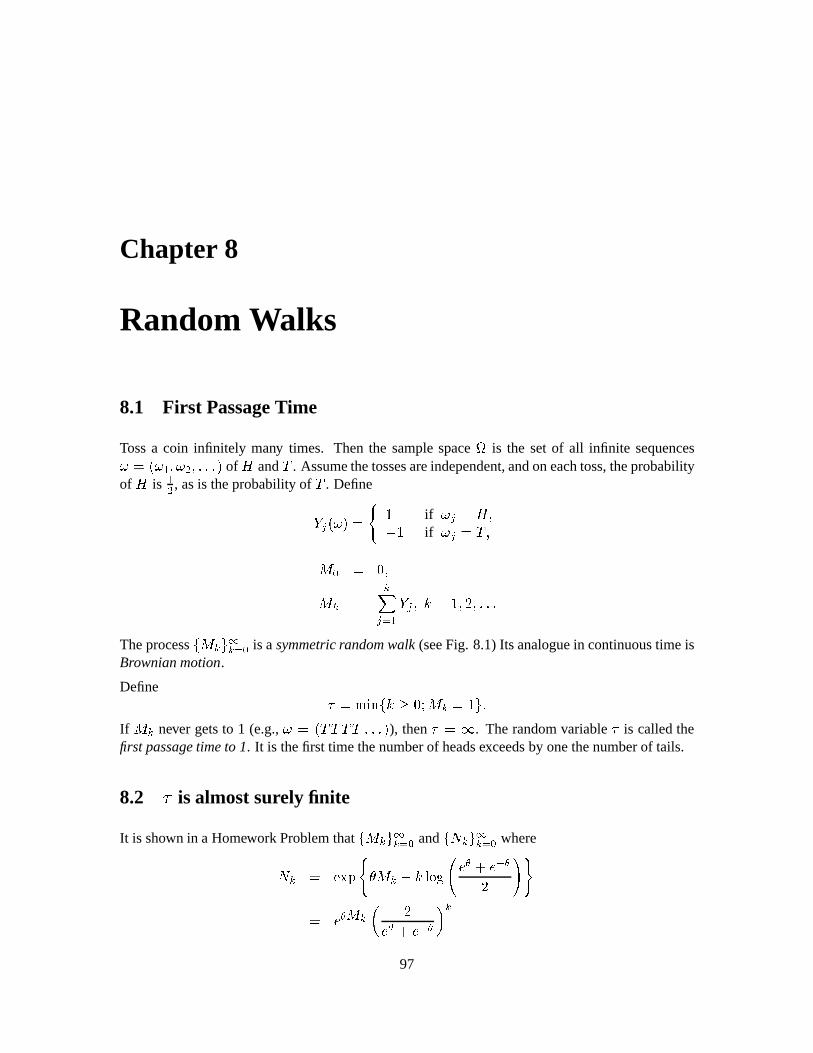
Chapter 8
RandomWalks
8.1 First PassageTime
Tossa coin infinitely many times. Then the samplespace¹ is the setof all infinite sequencesÝ ü Ý É © Ý » © IL of and . Assumethetossesareindependent,andoneachtoss,theprobabilityof is É» , asis theprobabilityof . DefineÇp Ý ü if Ý p ü © if Ý p ü © ú ü Ì © f ü fp mÊÉ Çp © û ü ©© LITheprocessj fl fm9ú is a symmetricrandomwalk (seeFig. 8.1)Its analoguein continuoustime isBrownianmotion.
Define n ü <j7û £ Ì fcü l If f never getsto 1 (e.g., Ý ü BLI ), then n ü ´ . Therandomvariable n is calledthe
first passagetimeto 1. It is thefirst time thenumberof headsexceedsby onethenumberof tails.
8.2 is almost surely finite
It is shown in a Homework Problemthat j f/l fm=ú and j fLl fm=ú where f ü f û ü f Ó Ö f97
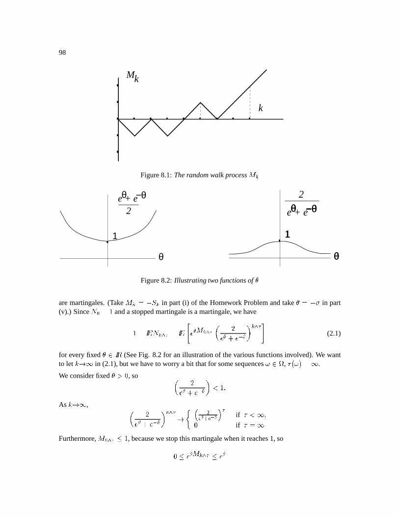
98
Mk
k
Figure8.1: Therandomwalkprocess f
e + e2
θ −θ
θ
1
θ
1
2
e + eθ −θ
Figure8.2: Illustratingtwo functionsof
aremartingales.(Take
f>ü Ï f in part (i) of theHomework Problemandtake
ü ! in part(v).) Since úcü andastoppedmartingaleis a martingale,wehave
ü s ~" fÜ w ü s ~$# fÜ w Ó Ö fÜ w&% (2.1)
for every fixed
Ñs ± (SeeFig. 8.2 for anillustrationof thevariousfunctionsinvolved). We wantto let û² ´ in (2.1),but wehave to worry a bit thatfor somesequencesÝ Ñ ¹ , n Ý ü ´ .
We considerfixed
' Ì , so Ó Ö ³ As û² ´ , Ó Ö fÜ w ² Ù »(*) È (,+) Ú w if n ³´ ©Ì if n ü ´Furthermore,
f$Ü w « , becausewestopthismartingalewhenit reaches1, soÌ « fÜ w «
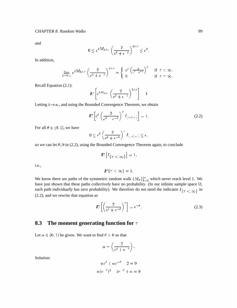
CHAPTER8. RandomWalks 99
and Ì « fÜ w Ó Ö f$Ü w « In addition, )f ² f$Ü w Ó Ö fÜ w ü Ù »( ) È ( +-) Ú w if n ³´ ©Ì if n ü ´ RecallEquation(2.1): s ~$# *.0/2143 Ó Ö fÜ w % ü Letting û² ´ , andusingtheBoundedConvergenceTheorem,we obtains ~ × Ó Ö w s uw65 x Øü (2.2)
For all
Ñ Ì © , we have Ì « Ó Ö w s uyw65 x « ©sowecanlet
87 Ì in (2.2),usingtheBoundedConvergenceTheoremagain,to concludes ~ s j7n ³´ l ¢ ü ©i.e., s 9'j7n ³´ lü We know therearepathsof thesymmetricrandomwalk j f/l fm=ú which never reachlevel 1. Wehave just shown that thesepathscollectivelyhave no probability. (In our infinite samplespace¹ ,eachpathindividually haszeroprobability). We thereforedo not needthe indicator s j7n ³´ l in
(2.2),andwerewrite thatequationass ~ × Ó Ö w Ø ü (2.3)
8.3 The momentgeneratingfunction for Let :Ñ Ì © I begiven.We wantto find
' Ì sothat: ü Ó ÖÒSolution: : : ü Ì: » : ü Ì
100
ü ;=< : »: We want
' Ì , sowemusthave ³ . Now Ì ³ : ³ , soÌ ³ : » ³ : ³ : » © : ³?> : » © > : » ³ : © < : »: ³ We takethenegativesquareroot: ü < : »: RecallEquation(2.3): s ~ × Ó Ö w Ø ü © ' Ì With :Ñ Ì © I and
' Ì relatedby ü < : »: ©: ü Ó Ö ©thisbecomes s ~ : w ü < : »: © Ì ³ : ³ (3.1)
We havecomputedthemomentgeneratingfunctionfor thefirst passagetime to 1.
8.4 Expectationof Recallthat s ~ : w ü < : »: © Ì ³ : ³ ©so @@ : s ~": w ü s ~ n: w É ü @@ : < : »: ü < : »: » < : »
CHAPTER8. RandomWalks 101
UsingtheMonotoneConvergenceTheorem,wecanlet :BA in theequations ~ n: w É ü < : »: » < : » ©to obtain s ~n ü ´ Thusin summary: n ü <j7û f ü l ©s 9'j7n ³´ lü ©s ~n ü ´ 8.5 The StrongMark ov Property
Therandomwalk processj fl fm9ú is aMarkov process,i.e.,s ~ randomvariabledependingonly on fÈÊÉ © fÈ » © LI ¤¦ f ü s ~ samerandomvariable ¤ f
In discretetime,this Markov propertyimpliestheStrongMarkovproperty:s ~ randomvariabledependingonly on w ÈÊÉ © w È » © II ¤ ¦ wIü s ~ samerandomvariable ¤ wv
for any almostsurelyfinite stoppingtime n .8.6 GeneralFirst PassageTimes
Define nC ü < j7û £ Ì fcü?D l © D ü ©E © IvThen n » nLÉ is thenumberof periodsbetweenthefirst arrival at level 1 andthefirst arrival at level2. Thedistributionof n » n É is thesameasthedistributionof n É (seeFig. 8.3),i.e.,s ~ : wGF wIH ü < : »: © :-Ñ Ì © L
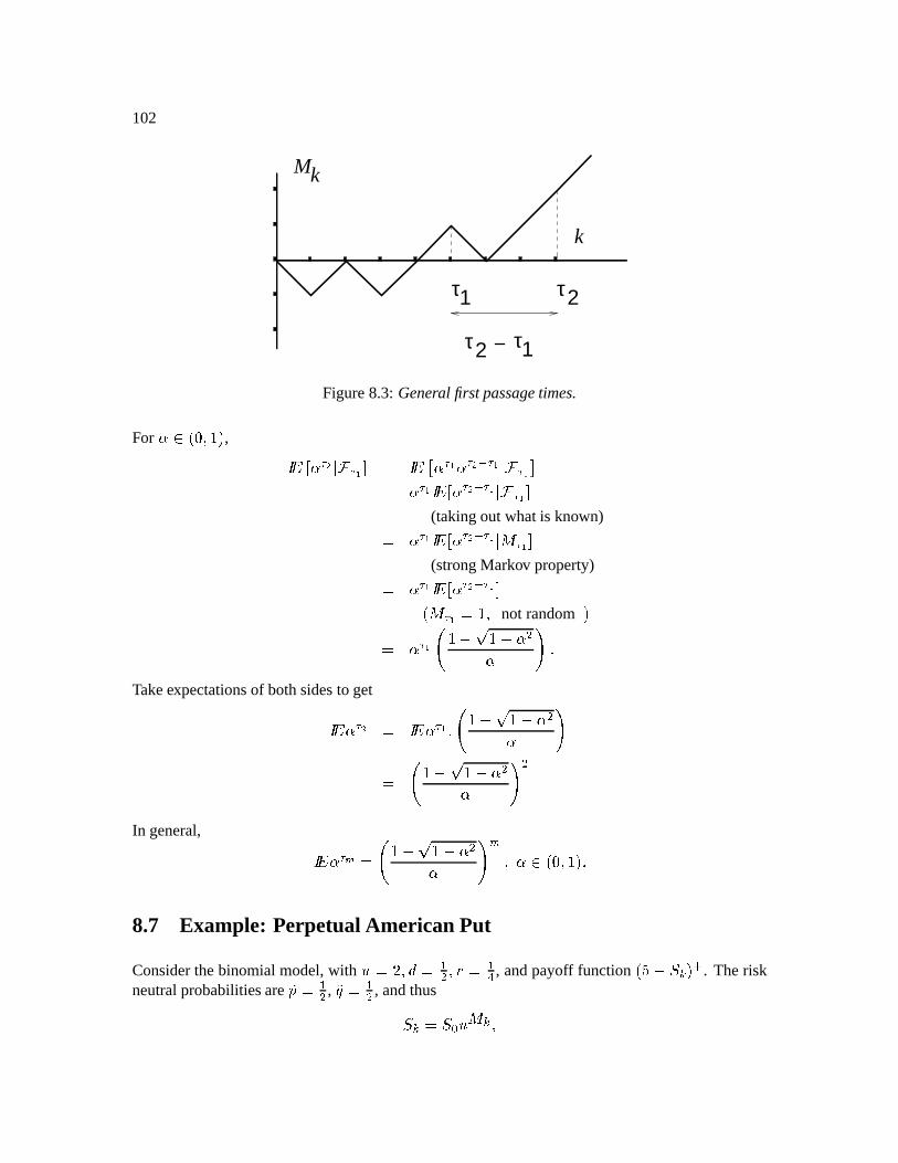
102
τ1
τ1
τ2
τ2
Mk
k
−
Figure8.3: General first passagetimes.
For :-Ñ Ì © L , s ~J: wGF ¤ ¦ wIH ü s ~LKM: wIH : w*F w2H ¤ ¦ w2HONü : wIH s ~J: w*F w2H ¤ ¦ w2H (takingout whatis known)ü : wIH s ~J: w*F w2H ¤ w2H (strongMarkov property)ü : wIH s ~J: w*F w2H wIH ü © not random ü : wIH < : »:
Takeexpectationsof bothsidesto gets ~ : w*F ü s ~": wIH P < : »: ü < : »: »In general, s ~ : w,Q ü < : »: C © :Ñ Ì © I 8.7 Example: Perpetual American Put
Considerthebinomialmodel,with R ü © @ ü É» © ü ÉS , andpayoff function UT Ï f È . Theriskneutralprobabilitiesare VW ü É» , VX ü É» , andthusÏ f ü Ï ú R f ©
CHAPTER8. RandomWalks 103
where f is a symmetricrandomwalk underthe risk-neutralmeasure,denotedby s 9 . SupposeÏ ú üZY . Herearesomepossibleexerciserules:
Rule 0: Stopimmediately. n úgü Ì ©[ | w ü .Rule 1: Stopassoonasstockpricefalls to 2, i.e.,at timen Égü <j7û fcü l Rule 2: Stopassoonasstockpricefalls to 1, i.e.,at timen » ü <j7û fcü l Becausethe randomwalk is symmetricunder s 9 , n C hasthe samedistribution under s 9 asthestoppingtime nC in theprevioussection.This observationleadsto thefollowing computationsofvalue.Valueof Rule 1: [ | w + H ü s ~ K K/ w + H UT Ï w + H È Nü UT È s ~ S \ w + H ¢ü ] _^ S \ »S \ü ] Valueof Rule 2: [ | w + F ü UT I È s ~ S \ w + F ¢ü Y É» »ü This suggeststhat theoptimalrule is Rule1, i.e., stop(exercisetheput) assoonasthestockpricefalls to 2, andthevalueof theput is ` » if Ï úgüZY .Supposeinsteadwe startwith Ï ú>üba , andstopthe first time the price falls to 2. This requires2down steps,sothevalueof this rule with this initial stockpriceis
UT È s ~ S \ w + F ¢ ü?] É» » ü ]Y In general,if Ï úcü p for someo £ , andwestopwhenthestockpricefalls to 2, theno downstepswill berequiredandthevalueof theoptionis
UT È s ~ S \ w +dc e,+ HMf ¢ üg] É» p É We define h p ü?] É» p É © o ü ©© ] © Iv
104
If Ï úKü p for some o « , then the initial price is at or below 2. In this case,we exerciseimmediately, andthevalueof theput ish p ü T p © o ü © Ì © © © vvProposedexerciserule: Exercisetheput whenever thestockprice is at or below 2. Thevalueofthis rule is givenby
h p aswe just definedit. Sincethe put is perpetual,the initial time is nodifferentfrom any othertime. This leadsusto makethefollowing:
Conjecture 1 Thevalueof theperpetualputat time û ish ¥Ï f .
How dowe recognizethevalueof anAmericanderivativesecuritywhenweseeit?
Therearethreepartsto theproofof theconjecture.Wemustshow:
(a)h ¥Ï f £ UT Ï f Èji û ©
(b) k S \ f h ¥Ï f ml fm=ú is asupermartingale,
(c) j h ¥Ï f lf$m=ú is thesmallestprocesswith properties(a)and(b).
Note: To simplify matters,weshallonly considerinitial stockpricesof theform Ï ú ü p , so Ï f isalwaysof theform p , with a possiblydifferento .Proof: (a). Justcheckthat h p ü?] É» p É £ UT p È for o £ ©h p ü T p £ UT p È for o « This is straightforward.
Proof: (b). We mustshow thath ¥Ï f £ s ~ S \ h Ï f$ÈÊÉ ¤ ¦ f ¢ü S \ É» h Ï f Õ S \ É» h É» Ï f By assumption,Ï fgü p for someo . We mustshow thath p £ »\ h p ÈÊÉ ; »\ h p É If o £ , then
h p üg] É» p É and»\ h p ÈÊÉ ; »\ h p É ü »\ ] É» p »\ ] É» p »ü ] × » \ Y »\ Ø É» p »ü ] É» É» p »ü h p
CHAPTER8. RandomWalks 105
If o ü , thenh p ü h ü?] and
»\ h p ÈÊÉ Õ »\ h p É ü »\ h Y ; » \ h Lü »\ ] É» »\ Yü ]on T an Tü É\ ³ h üg]Thereis a gapof size
S \.
If o « Ì , thenh p ü T p and
»\ h p ÈÕÉ Ê »\ h p É ü »\ UT p ÈÊÉ Õ »\ UT p É ü Y »\ Y tL p Éü Y p ³ h p ü T p Thereis a gapof size1. Thisconcludestheproofof (b).
Proof: (c). SupposejIÇ f/l i fm=ú is someotherprocesssatisfying:
(a’) Çf £ UT Ï f È i û ©(b’) j S \ f Ç fÄlfm=ú is a supermartingale.
We mustshow that Ç f'£ h Ï f i û (7.1)
Actually, sincetheput is perpetual,every time û is like everyothertime,soit will suffice to showÇ ú£ h ¥Ï ú © (7.2)
providedwelet Ï ú in (7.2)beany numberof theform p . With appropriate(but messy)conditioningon ¦ f , theproofwegiveof (7.2)canbemodifiedto prove (7.1).
For o « , h p ü T p ü UT p È ©soif Ï úqü p for someo « , then(a’) impliesÇ9ú £ pT p È ü h ¥Ï ú Supposenow that Ï ú ü p for someo £ , i.e., Ï ú£_Y . Letn ü <j7û Ï fcü lü <j7û fcü o l
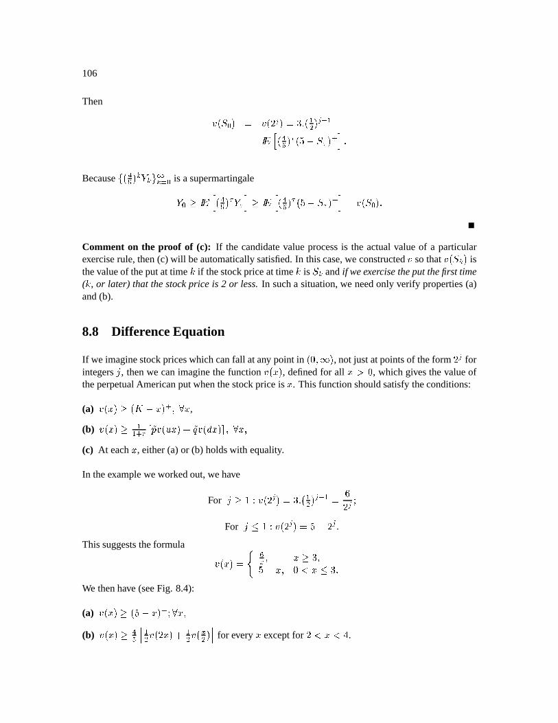
106
Then h ¥Ï ú ü h p üg] É» p Éü s ~ S \ w UT Ï w È ¢ Becausej S \ f Ç;f lfm=ú is asupermartingaleÇ ú'£ s ~ S \ w Ç w ¢ £ s ~® S \ w UT Ï w È ¢ ü h ¥Ï ú Comment on the proof of (c): If the candidatevalueprocessis the actualvalueof a particularexerciserule,then(c) will beautomaticallysatisfied.In thiscase,we constructed
hsothat
h ¥Ï f isthevalueof theputat time û if thestockpriceat time û is Ï f andif weexercisetheput thefirst time( û , or later) that thestock price is 2 or less.In sucha situation,we needonly verify properties(a)and(b).
8.8 Differ enceEquation
If we imaginestockpriceswhichcanfall atany point in Ì ©$´ , not justatpointsof theform p forintegerso , thenwe canimaginethe function
h ¥º= , definedfor all º ' Ì , which givesthevalueoftheperpetualAmericanputwhenthestockpriceis º . This functionshouldsatisfytheconditions:
(a)h ¥º= £ Î º= È © i º ,
(b)h ¥º9 £ ÉÉRÈrq ,VW h R º9 VX h @ º= © i º ©
(c) At eachº , either(a)or (b) holdswith equality.
In theexampleweworkedout,wehave
For o £ e h p üg] É» p É üts p For o « e h p ü T p
Thissuggeststheformula h ¥º9 ü vuw © º £=] ©T º © Ì ³ º « ] We thenhave (seeFig. 8.4):
(a)h ¥º= £ pT º9 È i º ©
(b)h ¥º9 £ S \ É» h º= É» h w » ¢ for every º exceptfor <³ º ³ Y .
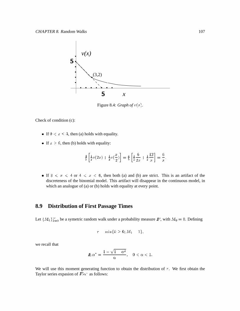
CHAPTER8. RandomWalks 107
5
5v(x)
x
(3,2)
Figure8.4: Graphofh º9 .
Checkof condition(c):x If Ì ³ º « ] , then(a)holdswith equality.x If º £ s , then(b) holdswith equality:S \ × É» h º=; É» h º Ø ü S \ × É» s º É» º Ø üysº x If ] ³ º ³ Y or Y ³ º ³ s , thenboth (a) and(b) arestrict. This is an artifact of thediscretenessof thebinomialmodel. This artifactwill disappearin thecontinuousmodel,inwhichananalogueof (a)or (b) holdswith equalityatevery point.
8.9 Distrib ution of First PassageTimes
Let j f/lfm=ú beasymetricrandomwalk underaprobabilitymeasures 9 , with úcü Ì . Definingn ü <j7û £ Ì fcü l ©
werecall that s ~ : w ü < : »: © Ì ³ : ³ We will usethis momentgeneratingfunction to obtainthe distribution of n . We first obtaintheTaylorseriesexpasionof s ~ : w asfollows:
108
z ¥º= ü < º © z Ì ü Ìz ¥º9 ü É» º9 É» © z Ì ü É»z · ¥º9 ü Y º9 ` » © z · Ì ü Yz · ¥º9 ü ] a º9 |F © z ·· Ì ü ]aLIz | p ¥º9 ü ~ ] LI - o ] p º9 c F e,+ HMfF ©z | p Ì ü ~ ] LI - o ] pü ~ ] LI - o ] p Y LI K o p É o I&ü Ù É» Ú » p É o & o ImTheTaylorseriesexpansionof
z ¥º9 is givenbyz º9 ü < ºü p m=ú o z | p Ì º pü p mÊÉ Ù É» Ú » p É o mo o I& º pü º p m » Ù É» Ú » p É o L o o º p Sowe have s ~ : w ü < : »:ü : z : » ü : p m » Ó : Ö » p É o I o o But also, s ~ : w ü p mÕÉ : » p É s 9'j/n ü o l
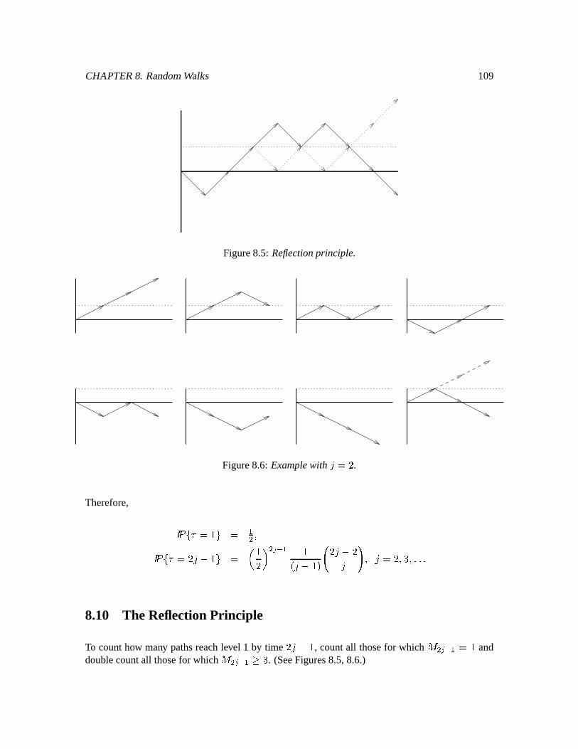
CHAPTER8. RandomWalks 109
Figure8.5: Reflectionprinciple.
Figure8.6: Examplewith o ü .Therefore, s 9'j7n ü l ü É» ©s 9'j7n ü o l ü Ó Ö » p É o I o o © o ü © ] © Lv8.10 The ReflectionPrinciple
To counthow many pathsreachlevel 1 by time o , countall thosefor which » p Éü and
doublecountall thosefor which » p Ég£] . (SeeFigures8.5,8.6.)
110
In otherwords,s 9'j7n « o l ü s 9'j » p Érü l s 9'j » p Ég£=]lü s 9'j » p É ü l s 9'j » p É £]l s 9'j » p É « ]lü s 9'j » p Éqü l For o £ , s 9'j7n ü o l ü s 9'j/n « o l s 9'j7n « o ]lü s 9'j » p Érü l s 9'j » p ` ü l ü s 9'j » p ` ü l s 9'j » p Éqü lü Ù É» Ú » p ` o ] m o Im o & Ù É» Ú » p É o Imo o Imü Ù É» Ú » p É o ] &o o I& Y o o I o II o ü Ù É» Ú » p É o ] &o o I& o o o II o ü Ù É» Ú » p É o &o o I&ü Ù É» Ú » p É o I o o
Chapter 9
Pricing in terms of Mark et Probabilities:The Radon-Nikodym Theorem.
9.1 Radon-Nikodym Theorem
Theorem 1.27(Radon-Nikodym) Let IP and s 9 be two probability measureson a space ¹z©¦ .Assumethat for every Ñ ¦ satisfying s 9 ü Ì , wealsohave s 9 ü Ì . Thenwe saythat s 9 is absolutelycontinuouswith respectto IP. Underthisassumption,there is a nonegativerandomvariable such that s 9 üg6 @ s 9 © i @Ñ ¦J© (1.1)
and is calledtheRadon-Nikodymderivativeof s 9 with respectto IP.
Remark 9.1 Equation(1.1) impliestheapparentlystrongerconditions ~ ü s ~Æ for every randomvariable for which s ~ ¤ ¤Ä³´ .
Remark 9.2 If s 9 is absolutelycontinuouswith respectto IP, andIP is absolutelycontinuouswithrespectto s 9 , we saythatIP and s 9 areequivalent.IPand s 9 areequivalentif andonly ifs 9 ü Ì exactly when s 9 ü Ì © i @Ñ ¦ If IP and s 9 areequivalentand is the Radon-Nikodymderivative of s 9 w.r.t. IP, then É is the
Radon-Nikodymderivativeof IPw.r.t. s 9 , i.e.,s ~ ü s ~ i © (1.2)s ~'Ç ü s ~·Ç i Ç (1.3)
(Let and Ç berelatedby theequationÇ ü to seethat(1.2)and(1.3)arethesame.)
111
112
Example9.1(Radon-Nikodym Theorem) Let ãvê>ê>èê<çGè ç ê>è çGç , the setof coin tosssequencesof length2. Let correspondto probability
æ for
êand
í for
ç, andlet correspondto probability
æíforê
and
æífor
ç. Then à)áFâÕã ð áÞñ ð áFñ , so à ê>ê^âÕãø è à ê<ç âÕãLÕè àùç ê>âÕãLÕè àùçGç âÕãå÷ ë
9.2 Radon-Nikodym Martingales
Let ¹ bethesetof all sequencesof Û coin tosses.Let IP bethemarketprobabilitymeasureandlet s 9 betherisk-neutralprobabilitymeasure.Assumes 9 Ý ' Ì © s 9 Ý ' Ì © i Ý Ñ ¹©sothatIP and s 9 areequivalent.TheRadon-Nikodymderivativeof s 9 with respectto IP is Ý ü s 9 Ý s 9 Ý DefinetheIP-martingale fü s ~Æ ¤ ¦ f © û ü Ì © © Lv © Û We cancheckthat f is indeeda martingale:s ~J f$ÈÊÉ ¤ ¦ f ü s ~§s ~J ¤ ¦ fÈÊÉ ¤ ¦ f ü s ~J ¤ ¦ f ü f Lemma 2.28 If is ¦ f -measurable,then s ~ ü s ~ f .Proof: s ~ ü s ~Æ ü s ~§s ~Æ ¤ ¦ f ü s ~§s ~J ¤ ¦ f ü s ~Æ f NotethatLemma2.28impliesthatif is ¦ f -measurable,thenfor any @Ñ ¦ f , s ~^§s ü s ~J f s ©or equivalently, @ s 9 ü f @ s 9
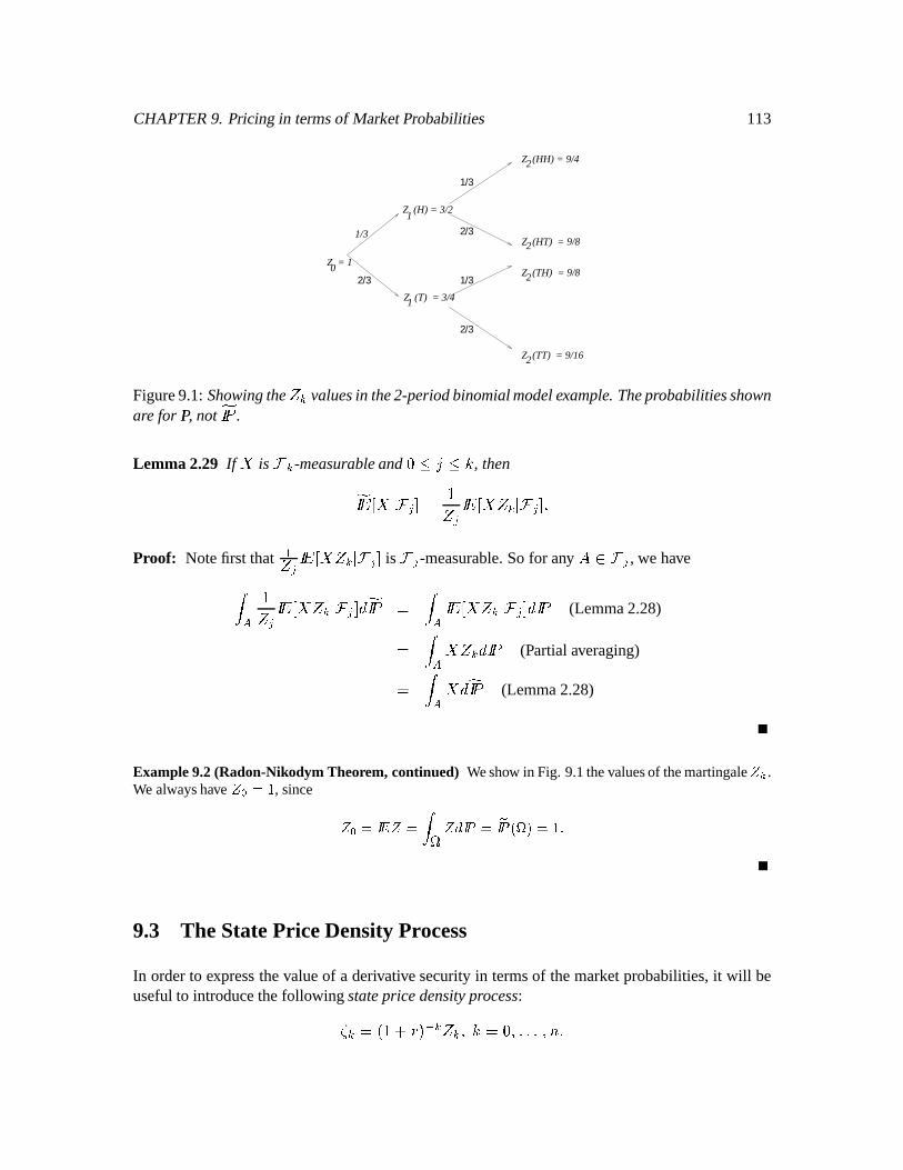
CHAPTER9. Pricingin termsof MarketProbabilities 113
0
1
1
2
2
2
2
Z = 1
Z (H) = 3/2
Z (T) = 3/4
Z (HH) = 9/4
Z (HT) = 9/8
Z (TH) = 9/8
Z (TT) = 9/16
2/3
1/3
1/3
2/3
1/3
2/3
Figure9.1:Showingthe f valuesin the2-periodbinomialmodelexample. Theprobabilitiesshownare for IP, not s 9 .
Lemma 2.29 If is ¦ f -measurableand Ì « o « û , thens ~ ¤ ¦ p ü Fp s ~ f ¤ ¦ p Proof: Notefirst that É p s ~ f ¤ ¦ p is ¦ p -measurable.Sofor any tÑ ¦ p , we have- Fp s ~ f ¤ ¦ p @ s 9 ü 6 s ~Æ f ¤ ¦ p @ s 9 (Lemma2.28)ü f @ s 9 (Partial averaging)ü @ s 9 (Lemma2.28)
Example9.2(Radon-Nikodym Theorem,continued) Weshow in Fig. 9.1thevaluesof themartingale .We alwayshave ã å , since ã ¡ ã £¢ ã à âÊã å ë9.3 The StatePrice DensityProcess
In orderto expressthevalueof a derivativesecurityin termsof themarketprobabilities,it will beusefulto introducethefollowing statepricedensityprocess:¤ f ü G7¾ f f © û ü Ì © IL © Û
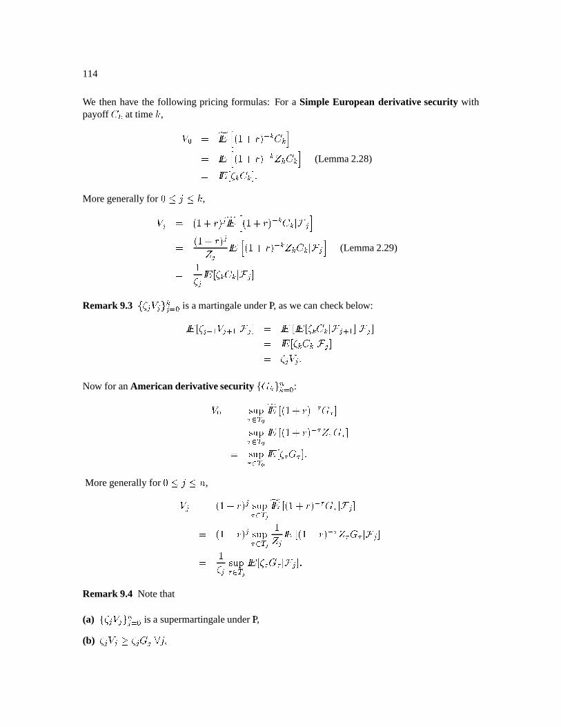
114
We thenhave the following pricing formulas: For a Simple Europeanderivative security withpayoff egf at time û , [ ú ü s ~ K/ f e f ¢ü s ~ K/ f f e f ¢ (Lemma2.28)ü s ~ ¤ f e f Moregenerallyfor Ì « o « û ,[ p ü G/ p s ~ K/ f e f ¤ ¦ p ¢ü G/ pFp s ~ K/ f f e f ¤ ¦ p ¢ (Lemma2.29)ü ¤ p s ~ ¤ f e f ¤ ¦ p Remark 9.3 j ¤ p [ p l fp m=ú is amartingaleunderIP, aswecancheckbelow:s ~ ¤ p ÈÕÉ [ p ÈÊÉ ¤ ¦ p ü s ~¨s ~ ¤ f e f ¤ ¦ p ÈÊÉ ¤ ¦ p ü s ~ ¤ f e f ¤ ¦ p ü ¤ p [ p Now for anAmerican derivative security jIk f/l i fm=ú :[ ú ü ¥E¦ w//I s ~ G/ w k wvü ¥E¦ w//I s ~ G/ w w k wvü ¥E¦ w//I s ~ ¤ w k wv Moregenerallyfor Ì « o « Û ,[ p ü G/ p ¥¦ w// e s ~ K/ w k w ¤ ¦ p ü G/ p ¥¦ w// e Fp s ~ G/ w w k w ¤ ¦ p ü ¤ p ¥E¦ w// e s ~ ¤ w k w ¤ ¦ p Remark 9.4 Notethat
(a) j ¤ p [ p l ip m=ú is a supermartingaleunderIP,
(b)¤ p [ p £ ¤ p$kp i o ©
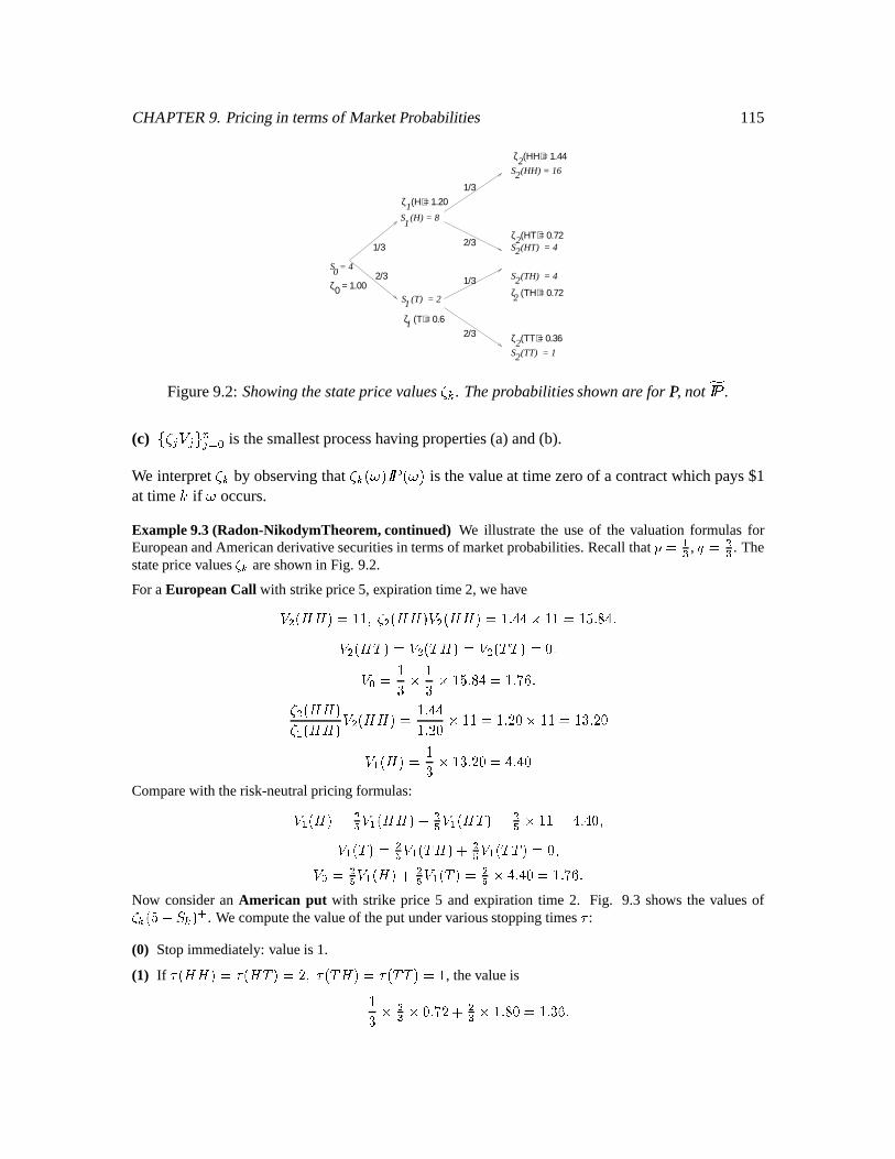
CHAPTER9. Pricingin termsof MarketProbabilities 115
S = 40
S (H) = 8
S (T) = 2
S (HH) = 16
S (TT) = 1
S (HT) = 4
S (TH) = 4
1
1
2
2
2
2
ζ = 1.00
ζ (Η) = 1.20
ζ (Τ) = 0.6
ζ (ΗΗ) = 1.44
ζ (ΗΤ) = 0.72
ζ (ΤΗ) = 0.72
ζ (ΤΤ) = 0.36
0
1
1
2
2
2
2
1/3
2/3
1/3
2/3
1/3
2/3
Figure9.2: Showingthestatepricevalues¤ f . Theprobabilitiesshownare for IP, not s 9 .
(c) j ¤ p [ p l ip m=ú is thesmallestprocesshaving properties(a)and(b).
We interpret¤ f by observingthat
¤ f Ý s 9 Ý is thevalueat time zeroof a contractwhich pays$1at time û if Ý occurs.
Example9.3(Radon-NikodymTheorem,continued) We illustrate the useof the valuationformulasforEuropeanandAmericanderivativesecuritiesin termsof marketprobabilities.Recallthat § ã æ , ¨ ã í . Thestatepricevalues© areshown in Fig. 9.2.
For a EuropeanCall with strikeprice5, expirationtime2, wehaveª í à ê^ê>âã åLå è © í àªê>ê>â ª í à ê>ê^âÕã å ë øIø¬« åIå ã åE ë øÅëª í àªê<ç âÕã ª í àùç ê>âÕã ª í àçGç âÊã®°ëª ã å¯ « å¯ « å ë øã å ë ° ÷ ë© í àªê>ê>â© æ àªê>ê>â ª í àªê>ê>âÕã å ë øIøå ë é ® « åLå ã å ë é ®« åLå ã å ¯ ë é ®ª æ àªê>âÕã å¯ « å ¯ ë é ®ãøë ø6®Comparewith therisk-neutralpricing formulas:ª æ$à ê>âÊã í± ª ævà ê>ê^â³² í± ª æ$à êç âÕã í ± « åLå ãSøÅë ø6®°èª æ¾àùç âÕã í± ª ævàç ê^â² í± ª ævàçGç âÊã´®Äèª ã í± ª ævà ê>â² í± ª ævàç âÕã í ± «'øÅë ø®ã å ë ° ÷ ëNow consideran American put with strike price 5 andexpiration time 2. Fig. 9.3 shows the valuesof©I à µ ì âG¶ . We computethevalueof theput undervariousstoppingtimes
ß:
(0) Stopimmediately:valueis 1.
(1) If
ßà ê>ê^âÕãßàªê<ç âÕã é èÕßàùç ê>âã-ßàùçGç âÕã å, thevalueiså¯ « í «"®Äë ° é ² í « å ë ® ã å ë ¯ ÷ ë
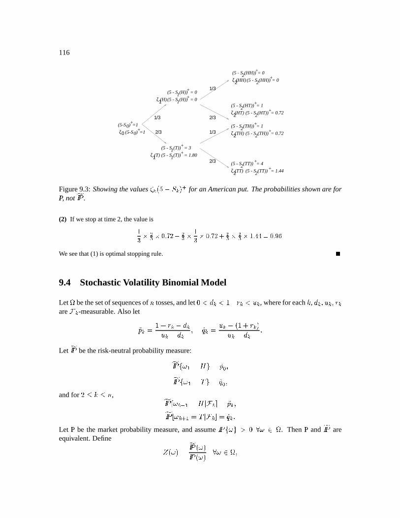
116
(5-S0)+=1ζ0
(5-S0)+=1
(5 - S1(H))+ = 0
(H)ζ1
(5 - S +(HH)) = 02(5 - S +(HH)) = 02ζ2(HH)
1/3
2/3
1/3
2/3
1/3
2/3
ζ1
(5 - S1+
(5 - S1+(T))
(T))
(T)
= 3
= 1.80
(5 - S1(H))+ = 0(5 - S +
2
(5 - S +2ζ2
(5 - S +2
(5 - S +2ζ2
(5 - S +2
(5 - S +2ζ2
(HT))
(HT) (HT))
= 1
= 0.72
(TH))
(TH) (TH))
= 1
= 0.72
(TT))
(TT) (TT))
= 4
= 1.44
Figure9.3: Showingthevalues¤ f UT Ï f È for anAmericanput. Theprobabilitiesshownare for
IP, not s 9 .
(2) If westopat time2, thevalueiså¯ « í «·®°ë° é ² í « å¯ «·®°ë° é ² í « í « å ë øIør㸮°ë ÷We seethat(1) is optimalstoppingrule.
9.4 StochasticVolatility Binomial Model
Let ¹ bethesetof sequencesof º tosses,andlet » ¼=½¿¾¼?ÀÁþ0¼Ä³¾ , wherefor eachÅ , ½¿¾ÆEÄr¾Æ¾are Ç ¾ -measurable.Also letÈÉ ¾¬Ê À£Á_Â8¾Ë´½¿¾Ä ¾ ˽ ¾ Æ ÈÌ ¾0Ê Ä³¾ËZÍ,ÀÁ=Â8¾&ÎÄ ¾ ˸½ ¾ ÏLet Ð Ñ betherisk-neutralprobabilitymeasure: Ð ÑÒ&ÓÔ£Ê?Õ×ÖØÊ ÈÉÙ ÆÐ Ñ Ò&ÓÔ£ÊZÚ0ÖØÊ ÈÌÙ Æandfor ÛÝÜ=ÅÃÜ=º , Ð Ñ·Þ Óß¾àBÔáÊ?Õ_â Ç·¾ãPÊ ÈÉ ¾Æ Ð Ñ Þ Ó ¾EàBÔ ÊZÚ â Ç ¾ ãPÊ ÈÌ ¾ ÏLet IP be the marketprobability measure,andassumeÐ ÑÒ&ÓÖ_äå»æÓèçL¹ . ThenIP and Ð Ñ areequivalent.Define é ÍêÓáÎ£Ê Ð ÑÃÍêÓáÎÐ Ñ·ÍëÓìÎ æÓíçî¹~Æ
CHAPTER9. Pricingin termsof MarketProbabilities 117é ¾ØÊ?Ð ïðÞ é â Ç ¾mãOÆÅ·Ê?»Æ8ÀÆ Ï8Ï&Ï ÆEº ÏWe definethemoney marketpriceprocessasfollows:ñ Ù ÊòÀÆñ ¾¬ÊóÍ,ÀÁ¾môPÔIÎ ñ ¾&ôõÔ6ƣŠÊòÀÆ Ï8ÏÏ Æº ÏNotethat
ñ ¾ is ö÷¾&ôõÔ -measurable.
We thendefinethestatepriceprocessto beø ¾ Ê Àñ ¾ é ¾ ƣŠÊ?»Æ ÏÏ8Ï ÆEº ÏAs beforethe portfolio processis Òùݾ6Öú ôPÔ¾û Ù . The self-financingvalue process(wealth process)consistsof ü Ù , thenon-randominitial wealth,andüð¾à ÔÊ?ù·¾ýB¾EàBÔ|Á?ÍþÀ|Á¾8ÎÍÿüð¾Ë¸ù·¾ý ¾8Î&ƣŠÊ?»Æ ÏÏ8Ï ÆEºÃË_À ÏThenthefollowing processesaremartingalesunder Ð Ñ : Àñ ¾ ý ¾ ú ¾Eû Ù and
Àñ ¾ üþ ú ¾û Ù Æandthefollowing processesaremartingalesunderIP:Ò ø ¾ý ¾oÖ ú ¾û Ù and Ò ø ¾&üð¾-Ö ú ¾Eû Ù ÏWe thushave thefollowing pricing formulas:
SimpleEuropeanderivative security with payoff ؾ at time Å : Ê ñ Ð ï ؾñ ¾ Ç Ê Àø Ð ï=Þ ø ¾Ø¾dâ Ç ãAmerican derivative security Ò"¾-Ö ú ¾Eû Ù : Ê ñ Ð ï ñ Ç Ê Àø Ð ïÞ ø â Ç ã ÏTheusualhedgingportfolio formulasstill work.
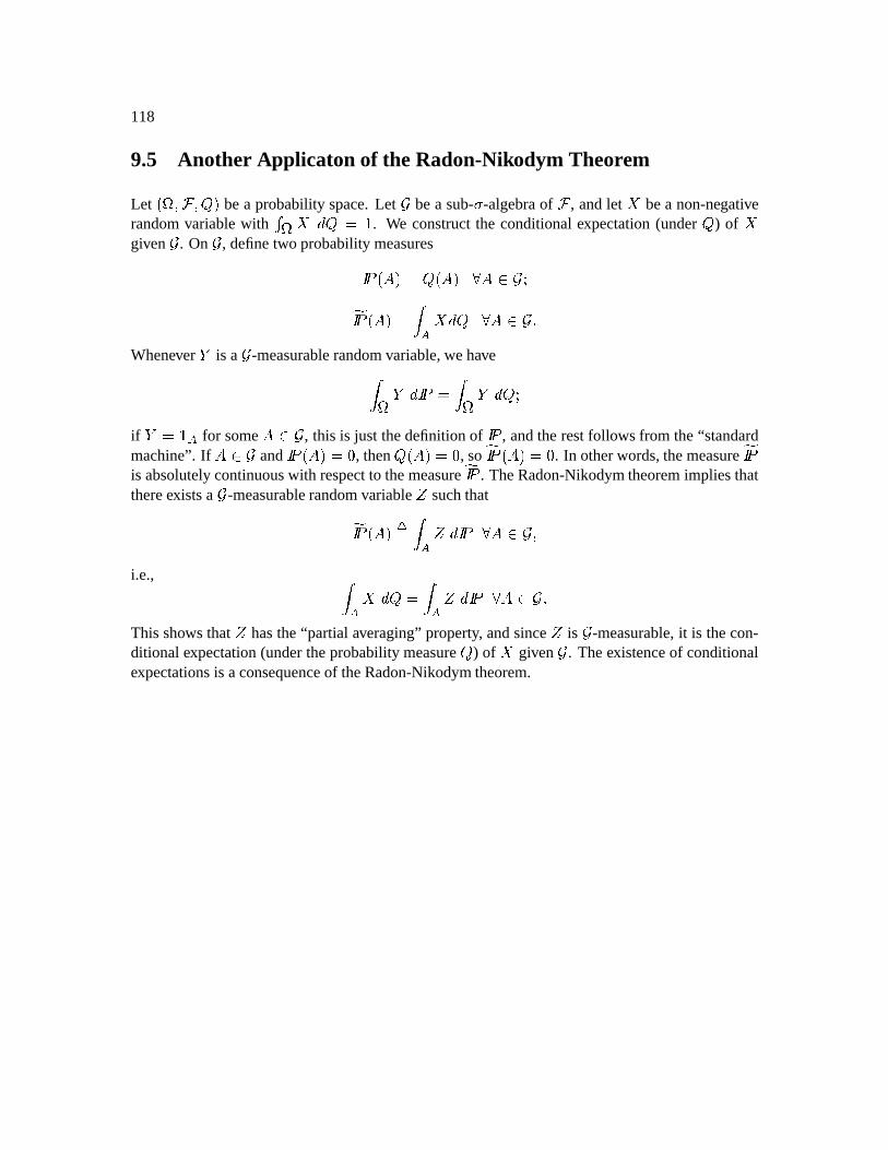
118
9.5 Another Applicaton of the Radon-Nikodym Theorem
Let ÍU¹~ÆIÇðÆ "Î bea probabilityspace.Let bea sub- -algebraof Ç , andlet ü bea non-negativerandomvariablewith ! ¹ ü ½" Ê À . We constructthe conditionalexpectation(under ) of ügiven . On , definetwo probabilitymeasuresÐ Ñ·Í$#ØÎÊ% Í&#¬Î æ'#Lç(*)Ð ÑÃÍ&#ØÎÊ,+- ü½" æ'#Lç( ÏWhenever . is a -measurablerandomvariable,wehave+ ¹ .ò½¿Ð Ñ?Ê + ¹ . ½"/)if .óÊ10 - for some#òç2 , this is just thedefinitionof Ð Ñ , andtherestfollowsfrom the“standardmachine”.If #Lç3 and Ð Ñ·Í$#ØÎÊ?» , then Í&#¬ÎÊ?» , so Ð ÑðÍ&#¬ÎÊ?» . In otherwords,themeasure Ð Ñis absolutelycontinuouswith respectto themeasure Ð Ñ . TheRadon-Nikodymtheoremimpliesthatthereexistsa -measurablerandomvariable
ésuchthat Ð ÑÃÍ&#ØÎ*4Ê + - é ½¿Ð Ñ æ'#Lç(Æ
i.e., +-üè½" Ê,+- é ½¿Ð Ñ æ'#Lç( ÏThis shows that
éhasthe“partial averaging”property, andsince
éis -measurable,it is thecon-
ditional expectation(undertheprobabilitymeasure ) of ü given . Theexistenceof conditionalexpectationsis aconsequenceof theRadon-Nikodymtheorem.
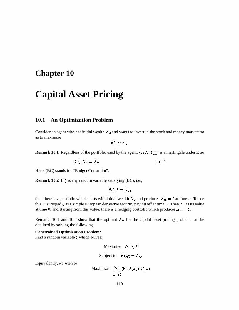
Chapter 10
Capital AssetPricing
10.1 An Optimization Problem
Consideranagentwhohasinitial wealth ü Ù andwantsto investin thestockandmoney marketssoasto maximize Ð ï6587:9ü ú ÏRemark 10.1 Regardlessof theportfolio usedby theagent,Ò ø ¾&üð¾-Ö<; ¾û Ù is amartingaleunderIP, soÐ ï ø ú ü ú ÊZü Ù Í&=>"ÎHere,(BC) standsfor “BudgetConstraint”.
Remark 10.2 If ? is any randomvariablesatisfying(BC), i.e.,Ð ï ø ú ?ÊZü Ù Æthenthereis a portfolio which startswith initial wealth ü Ù andproducesü ú Ê%? at time º . To seethis,just regard? asasimpleEuropeanderivativesecuritypayingoff at time º . Then ü Ù is its valueat time0, andstartingfrom thisvalue,thereis a hedgingportfolio which producesü ú Ê@? .Remarks10.1 and 10.2 show that the optimal ü ú for the capital assetpricing problemcan beobtainedby solvingthefollowing
ConstrainedOptimization Problem:Findarandomvariable? which solves:
Maximize Ð ïA5B7"9C?Subjectto Ð ï ø ú ?ÊZü Ù Ï
Equivalently, wewish toMaximize DÓ ¹ ÍE587:9F?rÍëÓáÎIÎÐ Ñ·ÍêÓáÎ
119
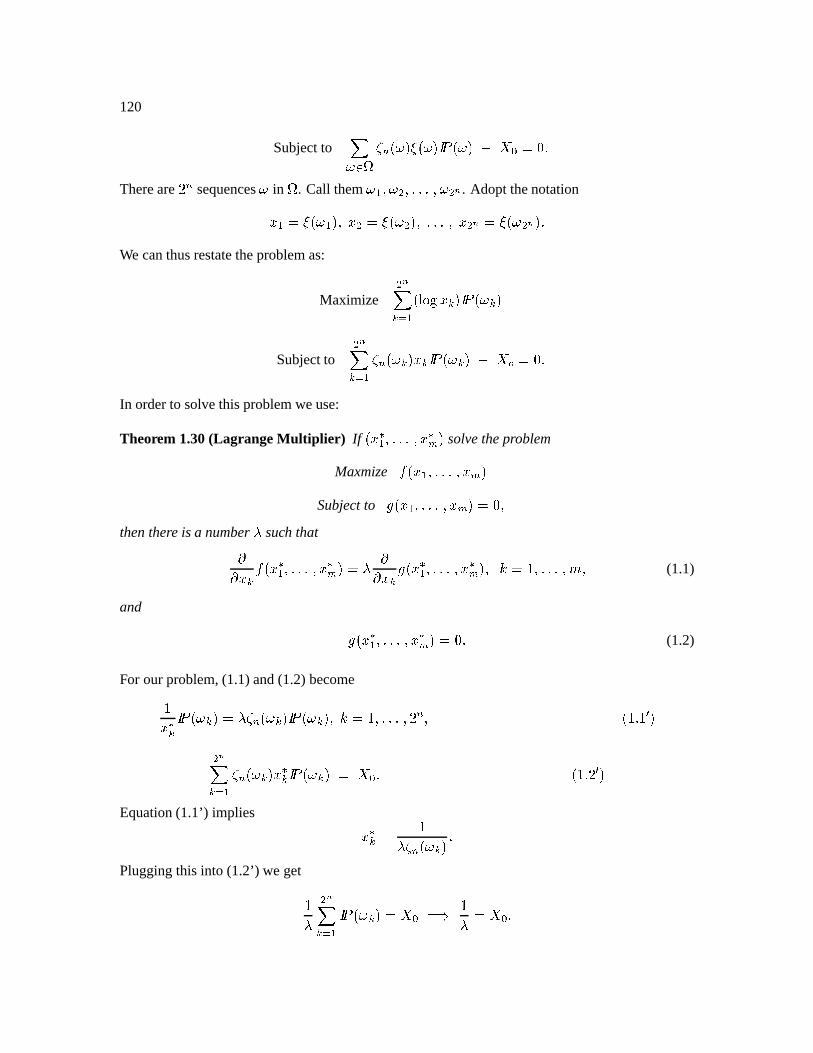
120
Subjectto DÓ ¹ ø ú ÍëÓáÎG?PÍêÓßÎ2Ð Ñ·ÍêÓáÎË ü Ù Ê?» ÏThereare Û ú sequencesÓ in ¹ . Call them ÓÔÆþÓFH6Æ ÏÏÏ ÆþÓFH I . Adopt thenotationJ ÔáÊK?PÍêÓÔEÎ&Æ J HÊ@?PÍêÓFH&ÎmÆ Ï8ÏÏ Æ J HLIÊ@?PÍêÓHLIÎ ÏWe canthusrestatetheproblemas:
MaximizeH ID¾EûBÔ ÍE587:9 J ¾ÎIÐ Ñ·ÍëÓá¾Î
SubjecttoH ID¾EûBÔ ø ú ÍêÓá¾Î J ¾Ð Ñ·ÍëÓì¾Î Ëvü/MÊ?» Ï
In orderto solve thisproblemweuse:
Theorem 1.30(LagrangeMultiplier) If Í JON Ô Æ ÏÏ8Ï Æ JONP Î solvetheproblem
Maxmize Q|Í J ÔÆ Ï8ÏÏ Æ J P ÎSubjectto R Í J Ô4Æ ÏÏÏ Æ J P ÎÊg»Æ
thenthere is a numberS such thatTT J ¾ QÍ J N Ô Æ Ï8ÏÏ Æ J NP ÎÊ1S TT J ¾ RBÍ J N Ô Æ ÏÏ8Ï Æ J NP ÎmÆ´Å ÊòÀÆ ÏÏÏ ÆU Æ (1.1)
and R Í J N Ô Æ ÏÏÏ Æ J NP ΣÊg» Ï (1.2)
For ourproblem,(1.1)and(1.2)becomeÀJ N¾ Ð Ñ·ÍêÓá¾6ÎÊ1S ø ú ÍêÓá¾8ÎIÐ Ñ·ÍêÓá¾8Î&ƣŷÊòÀoÆ ÏÏ8Ï ÆEÛ6úÆ Í,À Ï ÀV ÎH ID¾û Ô ø ú ÍêÓá¾8Î J N¾ Ð Ñ·ÍêÓá¾6ÎÊ ü Ù Ï Í,À Ï ÛVMÎEquation(1.1’) implies J N¾ Ê ÀS ø ú ÍêÓá¾Î ÏPluggingthis into (1.2’) we get ÀS H ID¾ûBÔ Ð Ñ·ÍëÓì¾ÎÊ ü Ù ÊXW ÀS ÊZü Ù Ï
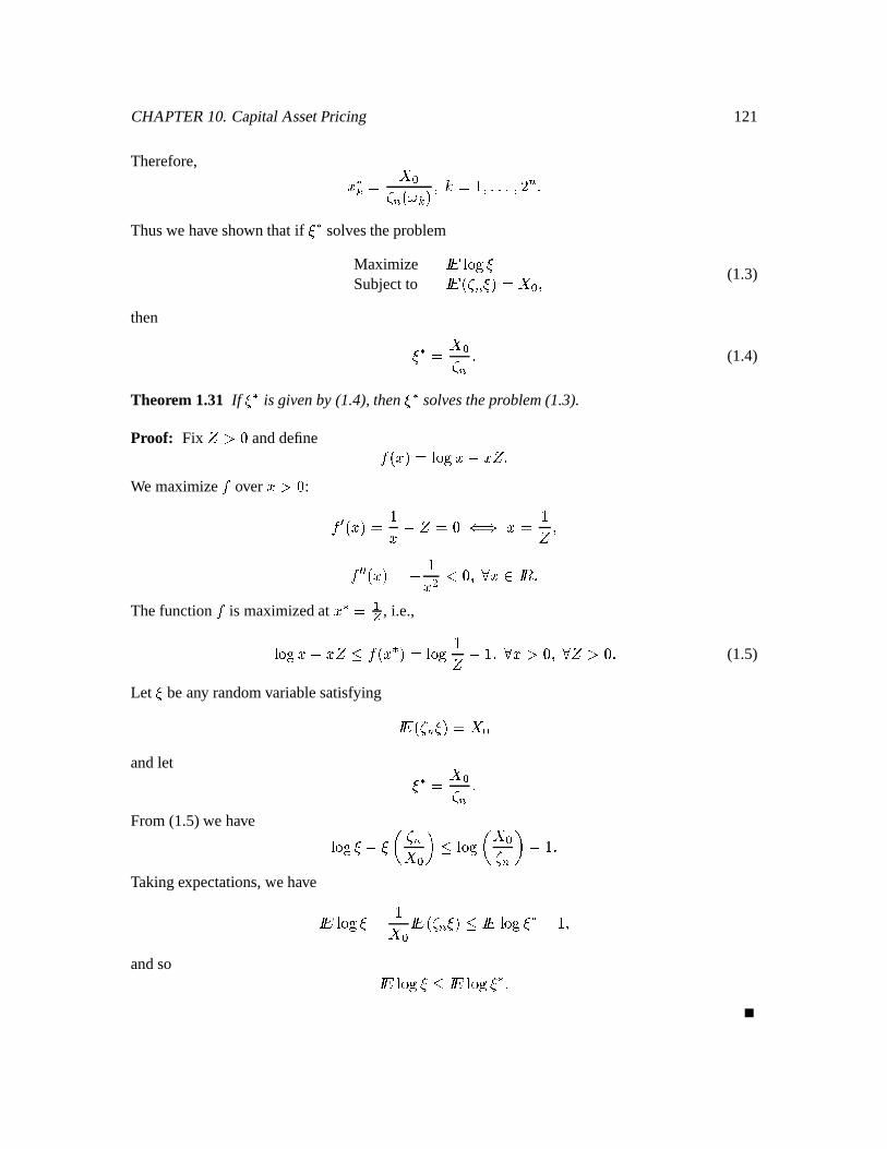
CHAPTER10. CapitalAssetPricing 121
Therefore, J N¾ Ê ü Ùø ú ÍêÓá¾8Î ÆÅ·ÊòÀÆ ÏÏ8Ï ÆEÛ ú ÏThuswe haveshown thatif ? N solvestheproblem
Maximize Ð ï6587:9F?Subjectto Ð ïÍ ø ú ?dÎÊZü Ù Æ (1.3)
then ? N Ê ü Ùø ú Ï (1.4)
Theorem 1.31 If ? N is givenby (1.4),then ? N solvestheproblem(1.3).
Proof: Fix
é ä=» anddefine QÍ J ÎÊ%587:9 J Ë J é ÏWe maximizeQ over J ä=» : QOVGÍ J ÎÊ ÀJ Ë é Êg»ZY[W J Ê Àé ÆQ V\V Í J ÎÊòË ÀJ H ¼=»ÆBæ J ç Ð ] ÏThefunction Q is maximizedat J N Ê Ô^ , i.e.,587:9 J Ë J é Ü_QÍ J N ÎÊ%587:9 Àé Ë_ÀoÆ÷æ J ä»ÆBæ é ä» Ï (1.5)
Let ? beany randomvariablesatisfying Ð ïÍ ø ú ?oÎÊ ü Ùandlet ? N Ê ü Ùø ú ÏFrom(1.5)we have 587:9F?Ë2?a` ø úü Ùcb Üd587:93` ü Ùø ú b ËÀ ÏTakingexpectations,wehave Ð ïA587:9?Ë Àü Ù Ð ïÍ ø ú ?oÎÜÐ ï6587:9e? N Ë=ÀÆandso Ð ïA587:9e? ÜÐ ï6587:9e? N Ï
122
In summary, capitalassetpricing worksasfollows: Consideran agentwho hasinitial wealth ü Ùandwantsto investin thestockandmoney marketsoasto maximizeÐ ï6587:9ü ú ÏTheoptimal ü ú is ü ú Êgfihø ú , i.e., ø ú ü ú ÊZü Ù ÏSince Ò ø ¾ ü ¾ Ö ú ¾û Ù is a martingaleunderIP, we haveø ¾müð¾ØÊgÐ ïÃÞ ø ú ü ú â Ç"¾mãPÊZü ٠ƣŷÊ?» Æ ÏÏ8Ï ÆEº÷Æso üð¾¬Ê ü Ùø ¾ Æandtheoptimalportfolio is givenbyù ¾ ÍëÓ Ô Æ Ï8ÏÏ Æ,Ó ¾ ÎÊ fihø ¾àBÔjÓ£Ô4Æ ÏÏ8Ï Æ,Ó¾k lnm Ë fihø ¾à ÔjÓ£ÔÆ ÏÏÏ Æ,Ó|¾ok mý ¾àBÔ-ÍêÓÔ4Æ ÏÏÏ Æ,Ó|¾oÆEÕ Î ËýB¾EàBÔ-ÍëÓ£Ô4Æ ÏÏ8Ï Æ,Ó¾ÆIÚ¬ÎÏ
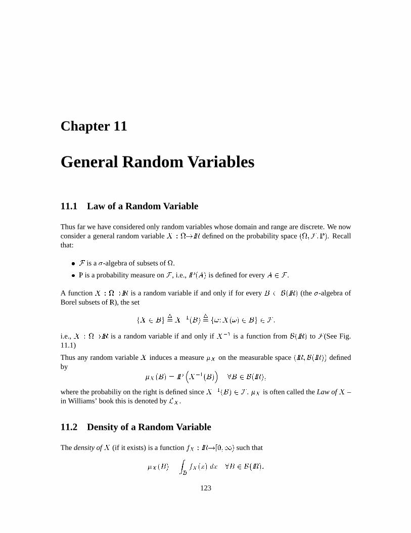
Chapter 11
GeneralRandomVariables
11.1 Law of a RandomVariable
Thusfar we have consideredonly randomvariableswhosedomainandrangearediscrete.We nowconsidera generalrandomvariable üqpõ¹rÐ ] definedon theprobabilityspaceÍU¹0ÆIÇÃÆLs£Î . Recallthat:t Ç is a -algebraof subsetsof ¹ .
tIP is aprobabilitymeasureon Ç , i.e., Ð Ñ·Í&#¬Î is definedfor every #?çÇ .
A function üup ¹nr_Ð ] is a randomvariableif andonly if for every = çKv ÍUÐ ]0Î (the -algebraofBorelsubsetsof IR), thesetÒü çw= Ö 4Ê ü ôõÔ Í&=Î 4ÊLÒ&Óx)2ü ÍëÓ|Îç(= Ö çÇîÆi.e., ü p¹nr_Ð ] is a randomvariableif andonly if ü ôPÔ is a function from v ÍpÐ ]0Î to Ç (SeeFig.11.1)
Thusany randomvariable ü inducesa measurey f on the measurablespaceÍUÐ ] ÆLvØÍpÐ ]0ÎIÎ definedby y f Í&=ÎÊ?Ð Ñ1zIü ôõÔ Í&=Î| æ'= ç3v ÍUÐ ]0Î&Æwheretheprobabiliyon theright is definedsinceü ôPÔ Í&=ÎçÇ . y f is oftencalledtheLawof ü –in Williams’ bookthis is denotedby f .
11.2 Densityof a RandomVariable
Thedensityof ü (if it exists) is a function Q f p¿Ð ]~rZÞJ»Æ_Î suchthaty f Í$=Î£Ê + Q f Í J ν J æ'=ç3vÍUÐ ]0Î Ï123
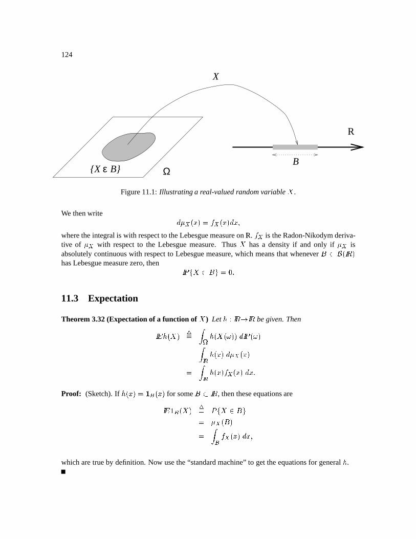
124
R
ΩBεB
X
X
Figure11.1: Illustratinga real-valuedrandomvariable ü .
We thenwrite ½:y f Í J ÎÊ,Q f Í J ÎI½ J Æwheretheintegral is with respectto theLebesguemeasureonIR. Q f is theRadon-Nikodymderiva-tive of y f with respectto the Lebesguemeasure. Thus ü hasa density if and only if y f isabsolutelycontinuouswith respectto Lebesguemeasure,which meansthatwhenever = çv ÍpÐ ]0ÎhasLebesguemeasurezero,then Ð ÑÒü çw= Ö Êg» Ï11.3 Expectation
Theorem 3.32(Expectationof a function of ü ) Let wpÐ ]~rÐ ] begiven.ThenÐ ï[÷ÍÿüÎ 4Ê + ¹ Íÿü=ÍêÓ£ÎIν¿Ð Ñ·ÍêÓáÎÊ +: Í J ν:y f Í J ÎÊ + Í J ÎLQ f Í J ν J ÏProof: (Sketch).If Í J ÎÊ10 Í J Î for some==Ð ] , thentheseequationsareÐ ï0 ÍÿüÎ 4Ê ÑÒü ç(= ÖÊ y f Í&=ÎÊ + Q f Í J ν J Æwhich aretrueby definition.Now usethe“standardmachine”to gettheequationsfor general .
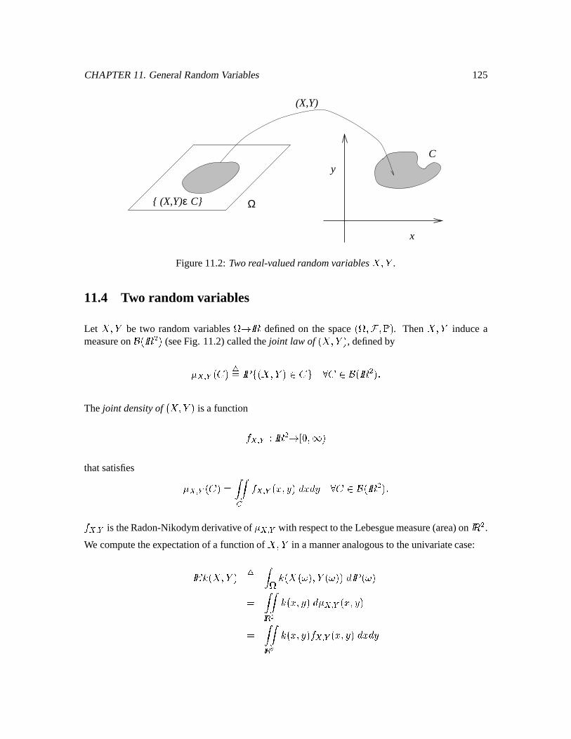
CHAPTER11. GeneralRandomVariables 125
Ωε
(X,Y)
(X,Y) C
C
x
y
Figure11.2:Tworeal-valuedrandomvariablesü Æ . .
11.4 Two random variables
Let ü Æ . be two randomvariables¹nr_Ð ] definedon the spaceÍp¹0ÆIÇÃÆLs£Î . Then ü ÆL. induceameasureon v ÍpÐ ] H Î (seeFig. 11.2)calledthe joint law of Íÿü ÆL.Î , definedbyy f k ÍE Î 4Ê?Ð ÑÒ Íÿü ÆL.Îç3·Ö æóç3v ÍpÐ ] H Î ÏThe joint densityof Íÿü Æ .Î is a functionQ f k pÐ ] H r?ÞJ»Æ_Îthatsatisfies y f k ÍE"ÎÊ +O+ Q f k Í J ƿν J ½ æ ç3v0ÍUÐ ] H Î ÏQ f k is theRadon-Nikodymderivativeof y f k with respectto theLebesguemeasure(area)on Ð ] H .We computetheexpectationof a functionof ü Æ . in a manneranalogousto theunivariatecase:Ð ï Å Íÿü Æ .Î 4Ê + ¹ Å Íÿü=ÍêÓ£Î&Æ .ðÍêÓáÎIν¿Ð Ñ·ÍêÓáÎÊ +O+ X Å Í J Æ¿Î ½"y f k Í J ÆdÎÊ +O+ Å Í J Æ¿ÎLQ f k Í J Æ¿Î÷½ J ½
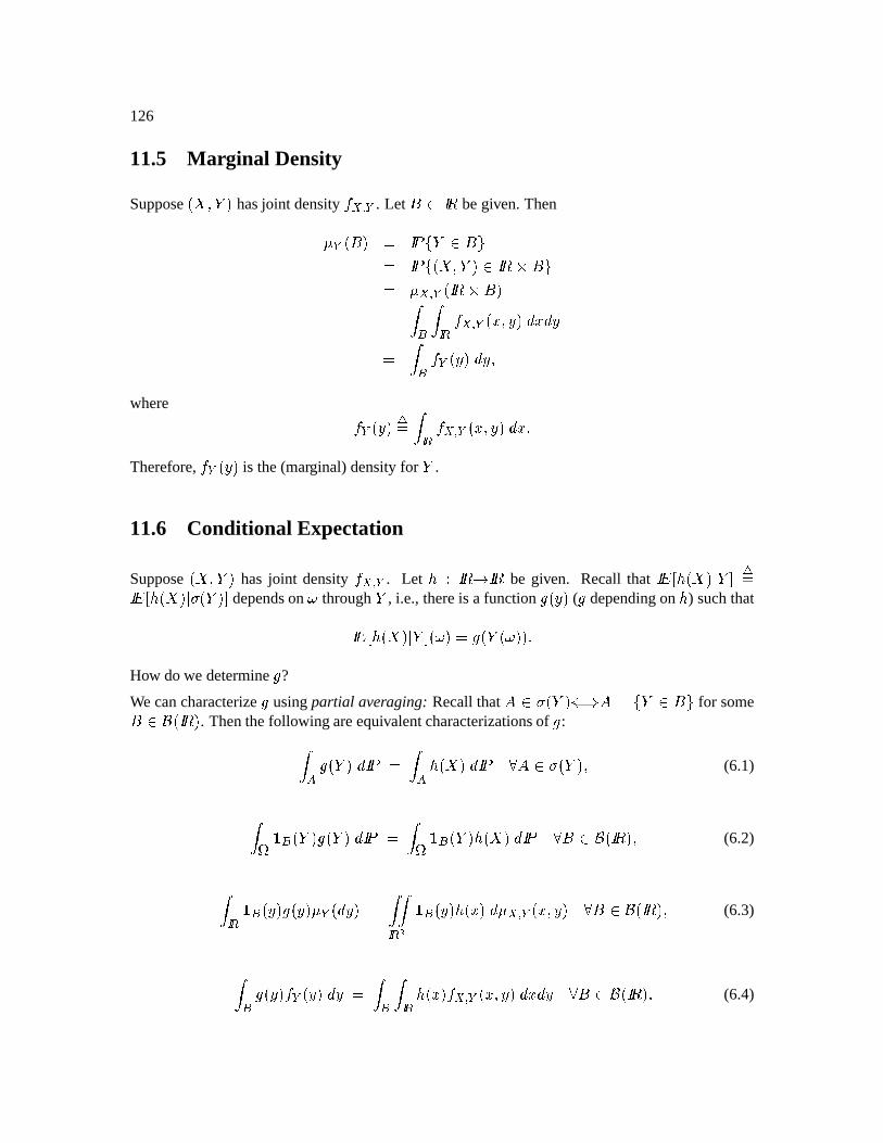
126
11.5 Mar ginal Density
SupposeÍÿü ÆL.Î hasjoint density Q f k . Let =gÐ ] begiven.Theny Í&=Î Ê Ð ÑÒ.bç(= ÖÊ Ð ÑÒ Íÿü ÆL. ÎçîÐ ]12= ÖÊ y f k ÍUÐ ]1=ÎÊ + + Q f k Í J Æ¿Î÷½ J ½Ê + Q Í$dνc³Æwhere Q Í&¿Î 4Ê +: Q f k Í J Æ¿Î ½ J ÏTherefore,Q Í&¿Î is the(marginal) densityfor . .
11.6 Conditional Expectation
SupposeÍ ü Æ ."Î hasjoint density Q f k . Let gp¬Ð ]~r=Ð ] be given. Recall that Ð ïÃÞ ÍÿüÎâ .ã 4ÊÐ ïÃÞ÷ÍÿüÎâ\ ÍE. Î*ã dependson Ó through. , i.e., thereis a function R Í&¿Î (R dependingon ) suchthatÐ ïÃÞ÷ÍÿüÎâ .ãþÍêÓ£ÎÊ@RBÍ. ÍêÓ£ÎIÎ ÏHow dowe determineR ?
We cancharacterizeR usingpartial averaging: Recallthat #òç2 ÍE.·ÎLY[W_#ZÊòÒo.bç= Ö for some=ç3vÍUÐ ]0Î . Thenthefollowing areequivalentcharacterizationsof R :+ ->RBÍ.Σ½¿Ð ÑÊ + -a Í üÎ÷½¿Ð Ñ æ'#Lç( ÍE.·Î&Æ (6.1)
+ ¹ 0 ÍE.·ÎGR ÍE.ν¿Ð Ñ Ê + ¹ 0 Í."ÎL÷ÍÿüÎ ½¿Ð Ñ æ'= çv ÍUÐ ]0ÎmÆ (6.2)
+: 0 Í&¿ÎGR Í&dÎy ÍU½cdÎ Ê +X+ X 0 Í&¿ÎL÷Í J ν"y f k Í J Æ¿Î æ'= ç3v ÍUÐ ]0Î&Æ (6.3)
+ RBÍ$dÎLQ Í&¿Î½ZÊ +/+" ÷Í J Î Q f k Í J Æ¿Î÷½ J ½ æ'=óçv~ÍpÐ ]0Î Ï (6.4)
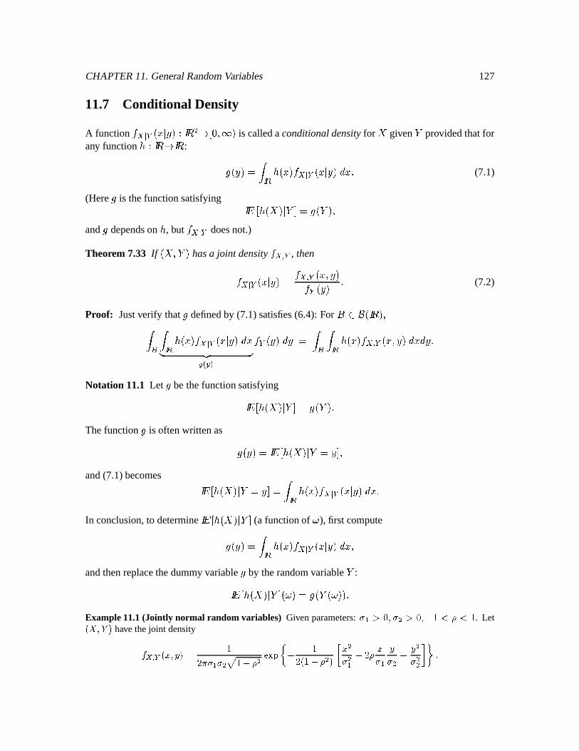
CHAPTER11. GeneralRandomVariables 127
11.7 Conditional Density
A function Q f~ Í J â\dÎ*pÐ ] H rZÞJ»Æ_Î is calledaconditionaldensityfor ü given . providedthatforany function (pÐ ]~rÐ ] : R Í&¿ÎÊ + Í J ÎLQ f~ Í J â\¿Î÷½ J Ï (7.1)
(Here R is thefunctionsatisfying Ð ï=Þ÷ÍÿüÎâ .¬ãPÊ@R ÍE. Î&Æand R dependson , but Q f~ doesnot.)
Theorem 7.33 If Íÿü Æ .Î hasa joint densityQ f k , thenQ f~ Í J â\¿Î Ê Q f k Í J Æ¿ÎQ Í&¿Î Ï (7.2)
Proof: Justverify that R definedby (7.1)satisfies(6.4): For = ç3v ÍpÐ ]0Î&Æ+/+: Í J ÎLQ f Í J â\dν J j8m Q Í$dνcZÊ +/+: Í J ÎLQ f k Í J Æ¿Î ½ J ½c ÏNotation 11.1 Let R bethefunctionsatisfyingÐ ïÃÞ÷ÍÿüÎâ .ãPÊ@RBÍ."Î ÏThefunction R is oftenwrittenas RBÍ&¿Î÷Ê?Ð ïÃÞ Í üÎ8â .?ÊZ6ã,Æand(7.1)becomes Ð ïÃÞ Í üÎ8â .íÊZ-ãPÊZ+ Í J ÎLQ f Í J â\¿Î ½ J ÏIn conclusion,to determineÐ ïÃÞ ÍÿüÎâ .ã (a functionof Ó ), first computeR Í&¿ÎÊ +: Í J ÎLQ f~ Í J â\¿Î÷½ J Æandthenreplacethedummyvariable by therandomvariable. :Ð ïÃÞ÷ÍÿüÎâ .ãþÍêÓ£ÎÊ@RBÍ. ÍêÓ£ÎIÎ ÏExample11.1(Jointly normal random variables) Givenparameters:n_ :¡|¢£_ :¡ ¤n¥£¦_§a¦Z¥ . Let¨ª© ¡G«x¬ have thejoint density®i¯ ° ¨²± ¡|³¬µ´ ¥¶· ¸c¢¹ ¥i¤/§ ¢FºL»¼ ¤ ¥¶ ¨ ¥i¤½§ ¢ ¬ ± ¢ ¢ ¤ ¶ § ± ³c¢n¾ ³ ¢ ¢¢ [¿
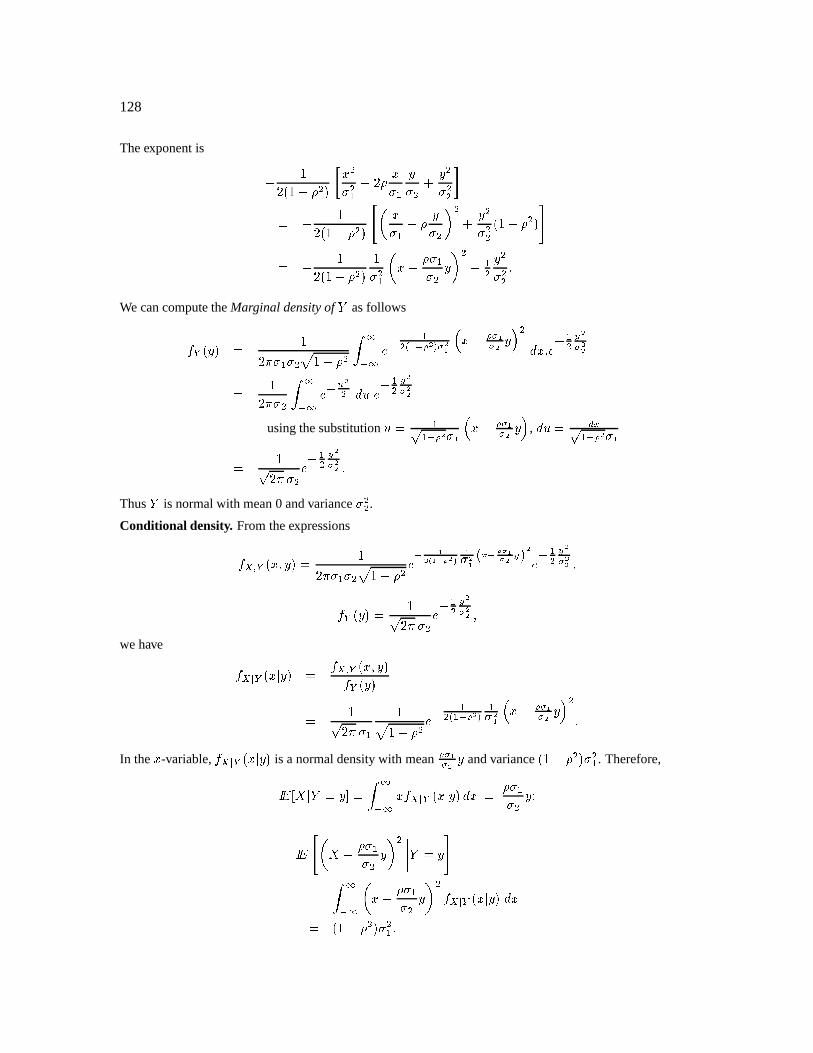
128
Theexponentis ¤ ¥¶ ¨ ¥i¤À§ ¢ ¬ ± ¢ ¢ ¤ ¶ § ± ³c¢ ¾ ³ ¢ ¢¢ ´ ¤ ¥¶ ¨ ¥i¤/§ ¢ ¬ÂÁ ` ± ¤½§ ³c¢ b ¢ ¾ ³ ¢ ¢¢ ¨ ¥i¤½§ ¢ ¬Eô ¤ ¥¶ ¨ ¥i¤/§ ¢ ¬ ¥ ¢ ` ± ¤ § ¢ ³ b ¢ ¤ ¢ ³ ¢ ¢¢ ¿We cancomputetheMarginal densityof « asfollows° ¨ ³o¬Ä´ ¥¶· c¢ ¹ ¥i¤/§ ¢ +2ÅÆ ÅÇ ¤ ¢ Ȫ ÆÊÉ|Ë&Ì8Í Ë Î z ± ¤ ÉÏÍ ÎÍ Ë ³ ¢*Ð ± ¿ Ç ¤ ¢Ñ ËÍ ËË´ ¥¶· ¢ +2ÅÆ Å2Ç ¤~Ò Ë¢
ÐÓ ¿ Ç ¤ ¢ Ñ ËÍ ËËusingthesubstitution
Ó ´ Ô ÆÉ Ë Î z ± ¤ ÉÏÍ ÎÍ Ë ³ ,
ÐÓ ´ ÕGÖÔ ÆÊÉ Ë Î´ ¥Ô ¶· ¢ Ç ¤ ¢Ñ ËÍ ËË ¿Thus « is normalwith mean0 andvariance ¢¢ .Conditional density. Fromtheexpressions®i¯ ° ¨²± ¡¸³o¬µ´ ¥¶· ¢ ¹ ¥i¤3§ ¢ Ç Æ ÎË$× ÎEØÙ Ë¸Ú Î Ë ÎcÛ Ö Æ ÙÏÜ ÎÜ Ë Ñ Ý Ë Ç ¤ ¢OÑ ËÍ ËË ¡ ° ¨ ³¬i´ ¥Ô ¶· c¢ Ç ¤ ¢OÑ ËÍ ËË ¡wehave ®eÞ ° ¨E±'ß ³o¬à´ ®i¯ ° ¨²± ¡¸³o¬° ¨ ³o¬´ ¥Ô ¶· ¥¹ ¥i¤/§ ¢ Ç ¤ ¢ Ȫ ÆÊÉ Ë Ì Ë Î z ± ¤ ÉGÍ ÎÍ Ë ³ ¢ ¿In the
±-variable,
®CÞ ° ¨²±Xß ³¬ is a normaldensitywith meanÉGÍ ÎÍ Ë ³ andvariance ¥i¤3§ ¢ ¬G ¢ . Therefore,á â~ã ©ß «_´³ä´ +2ÅÆ Å ± ®eÞ ° ¨²±Xß ³o¬
Ð ± ´ § ¢ ³:åá â Á ` © ¤ §< c¢ ³ b ¢ «_´æ³çô +2ÅÆ Å ` ± ¤ §c¢ ³ b ¢ ®CÞ ° ¨E±'ß ³¬ Ð ±´ ¨ ¥¤½§ ¢ ¬Ï ¢ ¿
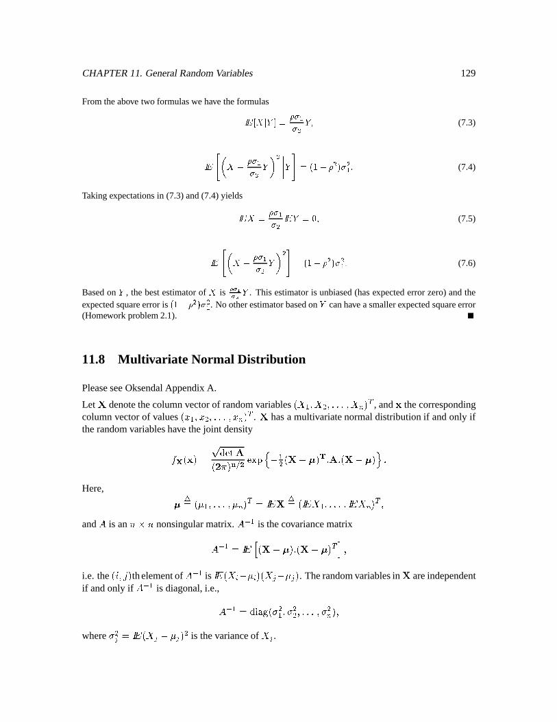
CHAPTER11. GeneralRandomVariables 129
Fromtheabove two formulaswehave theformulasá â~ã ©(ß «näÊ´ §< c¢ «è¡ (7.3)
á â Á ` © ¤ § ¢ « b ¢ « Ã ´ ¨ ¥i¤/§ ¢ ¬G ¢ ¿ (7.4)
Takingexpectationsin (7.3)and(7.4)yieldsá â © ´ §< ¢ á â «_´ :¡ (7.5)
á â Á ` © ¤ § ¢ « b ¢ ô ¨ ¥i¤/§ ¢ ¬G ¢ ¿ (7.6)
Basedon « , thebestestimatorof©
isÉÏÍ ÎÍ Ë « . This estimatoris unbiased(hasexpectederrorzero)andthe
expectedsquareerroris¨ ¥X¤a§ ¢ ¬Ï ¢ . No otherestimatorbasedon « canhave asmallerexpectedsquareerror
(Homework problem2.1).
11.8 Multi variate Normal Distrib ution
PleaseseeOksendalAppendixA.
Let é denotethecolumnvectorof randomvariablesÍÿü Ô ÆIü H Æ Ï8ÏÏ Æ2ü ú Î , and ê thecorrespondingcolumnvectorof values Í J ÔÆ J HÆ ÏÏ8Ï Æ J ú Î . é hasa multivariatenormaldistribution if andonly iftherandomvariableshave thejoint densityQoë"ÍEê÷ÎÊíì îïðXñÍ&òóBÎLô:õLö ï÷ ~ø Ë ÔH Í&éóË6ùÎ|ú Ïñ Ï Í&é Ë6ùáÎû ÏHere, ù 4ÊóÍEy Ô Æ ÏÏÏ Æ y ú Î Ê?Ð ï[é 4ÊóÍUÐ ïü Ô Æ ÏÏÏ ÆÐ ïü ú Î Æand # is an º2îº nonsingularmatrix. # ôPÔ is thecovariancematrix# ôõÔ Ê?Ð ïgüUÍ&é Ë6ùÎ Ï Í&éË6ùÎ µý Æi.e. the Í&þIÆGÿ Î thelementof # ôõÔ is Ð ïÍÿüË~y ÎÍ ü Ë~y Î . Therandomvariablesin é areindependentif andonly if # ôõÔ is diagonal,i.e.,# ôõÔ Ê î 9 Í& H Ô Æ HH Æ ÏÏ8Ï Æ Hú Î&Æwhere H Ê?Ð ïÍÿü Ë2y Î H is thevarianceof ü .
130
11.9 Bivariate normal distrib ution
Take ºÊ?Û in theabovedefinitions,andlet 4Ê Ð ïÍÿüjÔ|Ë2y÷ÔEÎÍÿü½H£ËAyH&Î ÷Ô XH ÏThus, # ôPÔ Ê Á H Ô BÔL µH BÔ XH HH à Æ
#ZÊ Ô j ÔIô m Ë j ÔIô mË j ÔIô m Ô j Ô2ô m Æì îïð #ZÊ À |Ô 'H ¹ ÀË H Æ
andwe have theformulafrom Example11.1,adjustedto accountfor thepossiblynon-zeroexpec-tations:Q f k f Í J Ô&Æ J HEÎÊ ÀÛ:óµ õÔL H ¹ ÀË H ï÷ Ë ÀÛ³Í,ÀË H Î Á Í J ÔË6y÷ÔEÎ H H Ô Ë Û Í J Ô Ë6y÷ÔEÎÍ J H£Ë2yµH8Î ÷ÔL µH Á Í J HË6yµH&Î H HH à Ï11.10 MGF of jointly normal random variables
Let Ê ÍUÄõÔ&ÆEÄOHÆ ÏÏÏ ÆÄ ú Î denotea column vector with componentsin Ð ] , and let é have amultivariatenormaldistributionwith covariancematrix # ôõÔ andmeanvector ù . Thenthemomentgeneratingfunctionis givenbyÐ ï Ï é Ê + ;ô ; Ï8ÏÏ + ;ô ; Ï é Q üÔ&ÆIü½HÆ ÏÏÏ Æ2ü ú Í J Ô4Æ J H8Æ ÏÏ8Ï Æ J ú ν J Ô ÏÏÏ ½ J úÊ ï÷ ø ÔH # ôõÔ Á ù û ÏIf any º randomvariablesüÔÆ2ü/H&Æ ÏÏÏ Æ2ü ú have this momentgeneratingfunction, thenthey arejointly normal,andwe canreadout themeansandcovariances.The randomvariablesarejointlynormalandindependentif andonly if for any realcolumnvector ÊóÍUÄÔÆ Ï8ÏÏ ÆEÄ ú Î Ð ï ë 4Ê?Ð ï ï÷ úD ûBÔ Ä ü ! "# Ê ï÷ úD ûBÔ Þ ÔH H Ä H Á_Ä y ã "# Ï
Chapter 12
Semi-ContinuousModels
12.1 Discrete-timeBrownian Motion
Let Ò. Ö ú ûBÔ beacollectionof independent,standardnormalrandomvariablesdefinedon Í%$0Æ2ÇðÆ s£Î ,whereIP is themarketmeasure. As beforewe denotethecolumnvector Í. ÔÆ Ï8ÏÏ Æ . ú Î by & . Wethereforehave for any realcolumvector îÊóÍUÄÔÆ ÏÏ8Ï ÆEÄ ú Î ,Ð ï('íÊ?Ð ï ï÷ ) úD ûBÔ Ä . "# Ê ï÷ ) úD ûBÔ ÔH Ä H "# ÏDefinethediscrete-timeBrownianmotion(SeeFig. 12.1):= Ù Ê » Æ=ؾ Ê ¾D ûBÔ . Æ ÅÝÊòÀÆ Ï8ÏÏ Æº ÏIf weknow . ÔÆL.XHÆ ÏÏ8Ï ÆL.õ¾ , thenweknow =~ÔÆ=£H8Æ ÏÏ8Ï Æ=¬¾ . Conversely, if weknow =0ÔÆ=xH8Æ Ï8ÏÏ Æ=¬¾ ,thenweknow . ÔÊZ=0ÔÆ .'HÊZ=£HËæ=~ÔÆ Ï8ÏÏ ÆL.õ¾ØÊ,=ؾ¬Ë6=¬¾&ôõÔ . DefinethefiltrationÇ Ù Ê Ò+*÷Æ,$ÖdÆÇ·¾ Ê £ÍE.BÔ4Æ .'H6Æ ÏÏÏ Æ .P¾8ÎÊZ £Í&=~ÔÆ=£HÆ ÏÏ8Ï Æ=¬¾ÎmÆ Å·ÊòÀoÆ ÏÏ8Ï ÆEº ÏTheorem 1.34 Ò<=¬¾6Ö ú ¾û Ù is a martingale(underIP).
Proof: Ð ï=Þ= ¾à Ô â Ç ¾ ã Ê Ð ï=Þ . ¾à Ô Á@= ¾ â Ç ¾ ãÊ Ð ï .P¾à Ô Á@=Ø¾Ê =ؾ Ï131
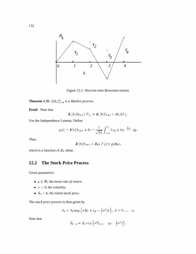
132
Y
Y
YY
1
2
34
k
Bk
0 1 2 3 4
Figure12.1:Discrete-timeBrownianmotion.
Theorem 1.35 Ò<= ¾ Ö ú ¾û Ù is a Markovprocess.
Proof: Notethat Ð ïÃÞ÷Í&=¬¾EàBÔEÎâ Ç·¾4ãPÊ?Ð ïÃÞ Í.P¾à Ô Á@=ؾ6Îâ Ç"¾ã ÏUsetheIndependenceLemma.DefineRBÍ%-&Î÷Ê?Ð ï[÷ÍE.P¾àBÔ Á.-&Î÷Ê Àì Û:ó + ;ô ; ÷Í&ØÁ/-&Î0 ô ÔH ½c ÏThen Ð ïÃÞ÷ÍE.P¾àBÔ Ád=ؾ6Îâ Ç ¾4ãPÊ@R Í&=ؾ8Î&Æwhich is a functionof =¬¾ alone.
12.2 The StockPrice Process
Givenparameters:t yçîÐ ] , themeanrateof return.t ä=» , thevolatility.t ý Ù ä=» , theinitial stockprice.
Thestock priceprocessis thengivenbyý ¾Êgý Ù ï÷ ø µ=ؾÁ?ÍEyË ÔH H ÎIÅ û Æ Å·Êg»Æ Ï8ÏÏ ÆEº ÏNotethat ý ¾àBÔáÊ?ý ¾ ï÷ ø O.P¾àBÔ|ÁÍy Ë ÔH H Î û Æ
CHAPTER12. Semi-ContinuousModels 133Ð ïðÞý ¾EàBÔâ Ç·¾mã Ê ý ¾8Ð ïÃÞ1 O.P¾àBÔ â Ç ¾&ã Ï 2 ô ÔH Ê ý ¾3 ÔH 2 ô ÔH Ê 2 ý ¾ ÏThus yîÊ%587:9 Ð ïÃÞJý ¾àBÔmâ Ç ¾4ãý ¾ Ê%587:9Ð ï ýB¾EàBÔý ¾ Ç ¾ Æand 4 (5 `:587:9 ýB¾EàBÔý ¾ b Ê 4 5 z O. ¾EàBÔ ÁLÍEyË ÔH H Î|·ÊZ H Ï12.3 Remainderof the Mark et
Theotherprocessesin themarketaredefinedasfollows.
Money marketprocess: ñ ¾¬Ê687 ¾ ÆÅ"Êg»ÆÀÆ ÏÏ8Ï Æº ÏPortfolioprocess:t ù Ù ÆùÃÔ&Æ ÏÏ8Ï ÆEù ú ôõÔÆt
Eachùݾ is Ç·¾ -measurable.
Wealthprocess:t ü Ù given,nonrandom.t
üð¾à Ô Ê ù·¾ý ¾àBÔ|Á9 7 Íÿüþ˴ùݾý ¾8ÎÊ ù·¾dÍUýB¾EàBÔáË: 7 ýB¾Î Á/ 7 üð¾tEachüþ is Ç·¾ -measurable.
Discountedwealthprocess: üþEàBÔñ ¾EàBÔ Êgù·¾ ` ý ¾àBÔñ ¾à Ô Ë ýB¾ñ ¾ b Á üð¾ñ ¾ Ï12.4 Risk-Neutral Measure
Definition 12.1 Let ; Ð Ñ bea probabilitymeasureon Í%$¬Æ2Ç Î , equivalentto themarketmeasureIP. Ifø ý ¾ñ ¾ û ú ¾û Ù is a martingaleunder; Ð Ñ , wesaythat ; Ð Ñ is a risk-neutral measure.
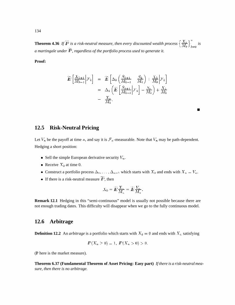
134
Theorem 4.36 If ; Ð Ñ is a risk-neutral measure, theneverydiscountedwealthprocessø üþñ ¾ û ú ¾û Ù is
a martingaleunder ;Ð Ñ , regardlessof theportfolio processusedto generateit.
Proof:
;Ð ïg üþEàBÔñ ¾àBÔ Ç·¾ Ê ; Ð ï ÿù·¾~` ý ¾àBÔñ ¾àBÔ Ë ý ¾ñ ¾ b Á ü ¾ñ ¾ Ç ¾ Ê ùݾ~` ; Ð ïg ý ¾àBÔñ ¾àBÔ Ç·¾ Ë ý ¾ñ ¾ b Á üð¾ñ ¾Ê üð¾ñ ¾ Ï12.5 Risk-Neutral Pricing
Let ú bethepayoff at time º , andsayit is Ç ú -measurable.Notethat
ú maybepath-dependent.
Hedgingashortposition:tSell thesimpleEuropeanderivativesecurity
ú .tReceive ü Ù at time0.
tConstructaportfolio processù Ù Æ ÏÏ8Ï ÆEù ú ôõÔ which startswith ü Ù andendswith ü ú Ê ú .tIf thereis a risk-neutralmeasure;Ð Ñ , thenü Ù Ê ;Ð ï ü úñ ú Ê ; Ð ï úñ ú Ï
Remark 12.1 Hedgingin this “semi-continuous”modelis usuallynot possiblebecausetherearenotenoughtradingdates.Thisdifficulty will disappearwhenwe goto thefully continuousmodel.
12.6 Arbitrage
Definition 12.2 An arbitrageis aportfolio whichstartswith ü Ù Ê?» andendswith ü ú satisfyingÐ Ñ·Íÿü ú=< »ÎÊòÀÆ÷Ð Ñ·Íÿü ú ä=»Îä» Ï(IP hereis themarketmeasure).
Theorem 6.37(FundamentalTheorem of AssetPricing: Easypart) If thereisarisk-neutral mea-sure,thenthere is noarbitrage.
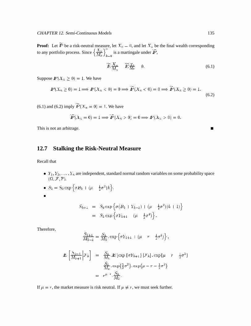
CHAPTER12. Semi-ContinuousModels 135
Proof: Let ; Ð Ñ bea risk-neutralmeasure,let ü Ù Ê» , andlet ü ú bethefinal wealthcorresponding
to any portfolio process.Sinceø ü ¾ñ ¾ û ú ¾û Ù is amartingaleunder; Ð Ñ ,; Ð ï ü úñ ú Ê; Ð ï6fih> h Ê?» Ï (6.1)
SupposeÐ Ñ·Íÿü ú?< »ÎÊòÀ . We haveÐ Ñ·Íÿü ú=< »ÎÊòÀÊ'W Ð Ñ·Íÿü ú ¼=»ÎÊ?»¬ÊXW ; Ð ÑðÍ ü ú ¼=»ÎÊ?»¬ÊXW ; Ð ÑÃÍÿü ú< »ÎÊ À Ï (6.2)
(6.1)and(6.2) imply ;Ð ÑðÍÿü ú Ê?»ÎÊòÀ . We have; Ð ÑðÍ ü ú Ê?»ÎÊòÀÊXW ; Ð ÑÃÍÿü ú ä=»ÎÊZ»0Ê'W Ð Ñ·Í ü ú ä »oΣÊ?» ÏThis is notanarbitrage.
12.7 Stalking the Risk-Neutral Measure
Recallthatt . ÔÆL.XHÆ ÏÏ8Ï ÆL. ú areindependent,standardnormalrandomvariablesonsomeprobabilityspaceÍ%$¬ÆIÇÆLs£Î .t ý ¾ Ê?ý Ù ï÷ ø µ= ¾ Á?ÍEyË ÔH H ÎIÅ û .týB¾EàBÔ Ê ý Ù ï÷ ø £Í$=ؾÁd.P¾àBÔ4ÎõÁÍy Ë ÔH H Î8ÍUÅ0ÁZÀÎ ûÊ ý ¾ ï÷ ~ø O.P¾àBÔ|ÁÍy Ë ÔH H Îû Ï
Therefore, ý ¾àBÔñ ¾àBÔ Ê ýB¾ñ ¾ ÏLï÷ ø X. ¾EàBÔ Á?ÍEyîËÂ¬Ë ÔH H Î û ÆÐ ï ýB¾EàBÔñ ¾EàBÔ Çð¾ Ê ý ¾ñ ¾ Ï Ð ï_Þ ï÷ Ò .õ¾EàBÔ8Öáâ Ç·¾&ã Ï ï÷ ÒyîËÂ¬Ë ÔH H ÖÊ ý ¾ñ ¾ ÏLï÷ Ò ÔH H Ö ÏLï÷ Òoy Ë¸Â¬Ë ÔH H ÖÊ 2 ô 7 Ï ýB¾ñ ¾ ÏIf yîÊ? , themarketmeasureis risk neutral.If y9@Êg , wemustseekfurther.
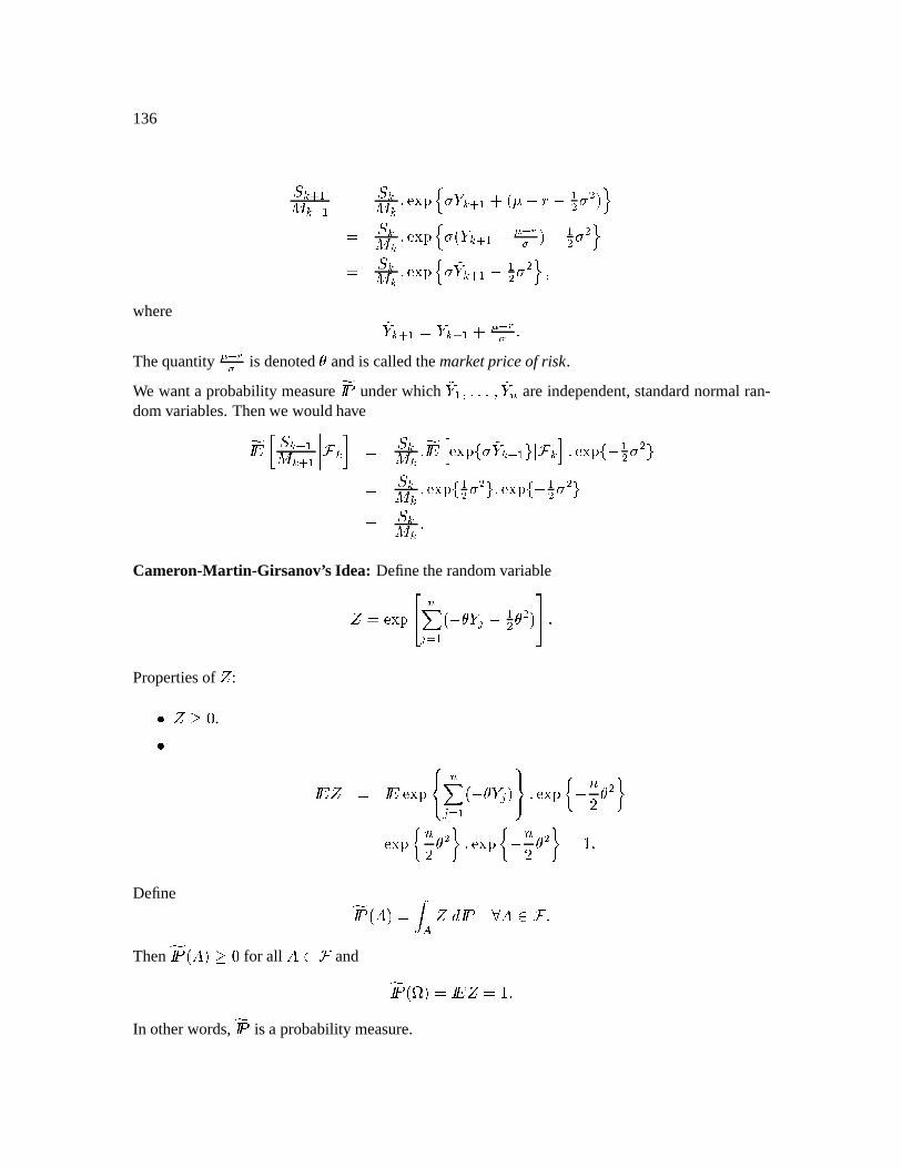
136
ý ¾àBÔñ ¾EàBÔ Ê ýB¾ñ ¾ ÏLï÷ xø .õ¾EàBÔÁÍEyËÂ¬Ë ÔH H ÎûÊ ýB¾ñ ¾ ÏLï÷ ø |Í.P¾à ÔÁA2 ô 7 ÎË ÔH H ûÊ ýB¾ñ ¾ ÏLï÷ ø È.õ¾EàBÔË ÔH H û Æwhere
È.P¾àBÔáÊ%.õ¾EàBÔ|ÁB2 ô 7 ÏThequantity 2 ô 7 is denotedC andis calledthemarketpriceof risk.
We wanta probabilitymeasure; Ð Ñ underwhich
È.BÔÆ Ï8ÏÏ Æ È. ú areindependent,standardnormalran-domvariables.Thenwe wouldhave;Ð ï ý ¾EàBÔñ ¾à Ô Ç ¾ Ê ý ¾ñ ¾ Ï ;Ð ï ü ï÷ Ò< È. ¾à Ô Ö â Ç ¾ ý Ï ï÷ ÒdË ÔH H ÖÊ ý ¾ñ ¾ ÏLï÷ Ò ÔH H Ö ÏLï÷ ÒdË ÔH H ÖÊ ý ¾ñ ¾ ÏCameron-Martin-Girsanov’ s Idea: Definetherandomvariableé Ê ï÷ úD û Ô Í,ËDCo. Ë ÔH C H Î ÏPropertiesof
é:t é < » .t
Ð ï é Ê Ð ï ï÷ úD ûBÔ Í,ËDC. Î "# ÏLï÷ Ë º Û C H Ê ï÷ º Û C H Ï ï÷ Ë º Û C H ÊòÀ ÏDefine ; Ð ÑðÍ&#¬ÎÊZ+- é ½¿Ð Ñ æ'#çjÇ ÏThen ; Ð ÑÃÍ&#ØÎ < » for all #çjÇ and ; Ð ÑðÍ%$ÎÊgÐ ï é ÊòÀ ÏIn otherwords, ;Ð Ñ is a probabilitymeasure.
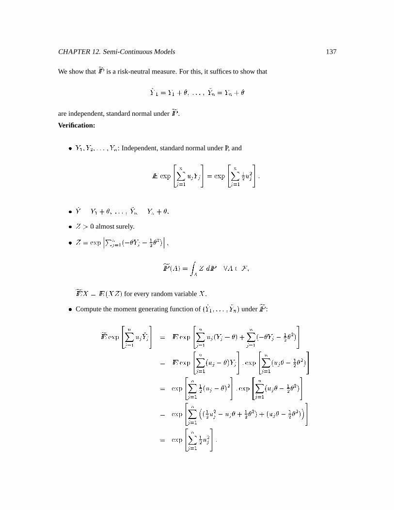
CHAPTER12. Semi-ContinuousModels 137
We show that ; Ð Ñ is a risk-neutralmeasure.For this, it sufficesto show thatÈ. Ô Ê%. Ô Á9CÆ ÏÏ8Ï Æ È. ú Ê%. ú Á.Careindependent,standardnormalunder; Ð Ñ .
Verification:t . ÔÆL.XHÆ ÏÏ8Ï ÆL. ú : Independent,standardnormalunderIP, andÐ ï ï÷ úD ûBÔ Ä . Ê ï÷ úD ûBÔ ÔH Ä H Ït È. Ê%.BÔ Á9CÆ ÏÏ8Ï Æ È. ú Ê%. ú Á9C Ït é ä» almostsurely.t é Ê ï÷ üFE ú ûBÔ Í,ËDC. Ë ÔH C H Î ý Æ; Ð ÑÃÍ&#¬ÎÊ + - é ½¿Ð Ñ æ'#LçÇÆ; Ð ï0üyÊ?Ð ïÍÿü é Î for every randomvariableü .tComputethemomentgeneratingfunctionof Í È. Ô Æ ÏÏÏ Æ È. ú Î under;Ð Ñ :
;Ð ï ï÷ úD ûBÔ Ä È. Ê Ð ï ï÷ úD ûBÔ Ä ÍE. Á.C6Î Á úD û Ô Í,ËDCo. Ë ÔH C H Î Ê Ð ï ï÷ úD ûBÔ ÍUÄ Ë:CÎ|. ÏLï÷ úD ûBÔ ÍUÄ CØË ÔH C H Î Ê ï÷ úD ûBÔ ÔH ÍpÄ Ë:CÎ H ÏLï÷ úD û Ô ÍUÄ C¬Ë ÔH C H Î Ê ï÷ úD ûBÔ zÍ ÔH Ä H Ë´Ä CÁ ÔH C H Î Á?ÍUÄ C0Ë ÔH C H Î| Ê ï÷ úD ûBÔ ÔH Ä H Ï
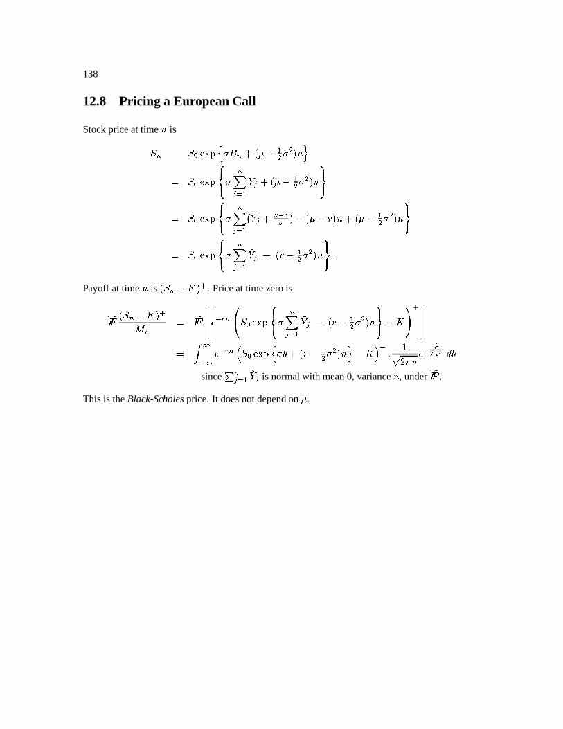
138
12.8 Pricing a EuropeanCall
Stockpriceat time º isý ú Ê ý Ù ï÷ ø X= ú ÁÍy Ë ÔH H Î2º ûÊ ý Ù ï÷ ) úD ûBÔ . Á?ÍEyË ÔH H ÎIº "#Ê ý Ù ï÷ úD ûBÔ ÍE. ÁA2 ô 7 ÎË=ÍEyË´Â6ÎIºÁÍEyË ÔH H ÎIº "#Ê ý Ù ï÷ ) úD ûBÔ È. Á ÍpÂË ÔH H Î2º "# ÏPayoff at time º is ÍUý ú Ë:G Î à . Priceat time zerois
;Ð ï ÍUý ú Ë:G Î àñ ú Ê ; Ð ï ô 7 úIHJrý Ù ï÷ úD ûBÔ È. ÁÍUÂ¬Ë ÔH H ÎIº "# ËKGMLN à Ê + ;ô ; ô 7 ú z ý Ù ï÷ >ø O- ÁLÍUÂË ÔH H ÎIºiû·Ë:G à Ï Àì Û"ó º ôQP I ½R-since E ú ûBÔ È. is normalwith mean0, varianceº , under; Ð Ñ .
This is theBlack-Scholesprice.It doesnot dependon y .
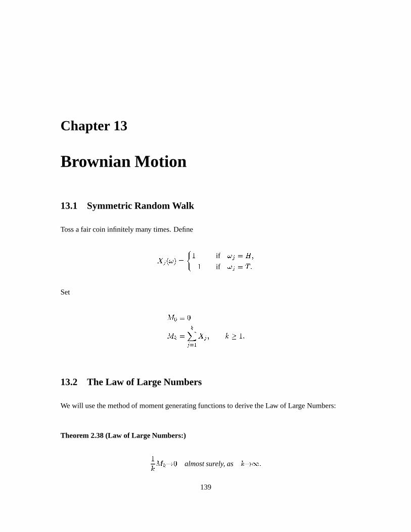
Chapter 13
Brownian Motion
13.1 Symmetric RandomWalk
Tossa fair coin infinitely many times.Define
ü ÍêÓ£ÎÊ À if Ó Ê?Õ ÆË0À if Ó ÊZÚ ÏSet ñ Ù Ê?»ñ ¾ Ê ¾D ûBÔ ü Æ Å < À Ï13.2 The Law of Lar geNumbers
We will usethemethodof momentgeneratingfunctionsto derive theLaw of LargeNumbers:
Theorem 2.38(Law of Large Numbers:)ÀÅ ñ ¾r=» almostsurely, as Ård Ï139
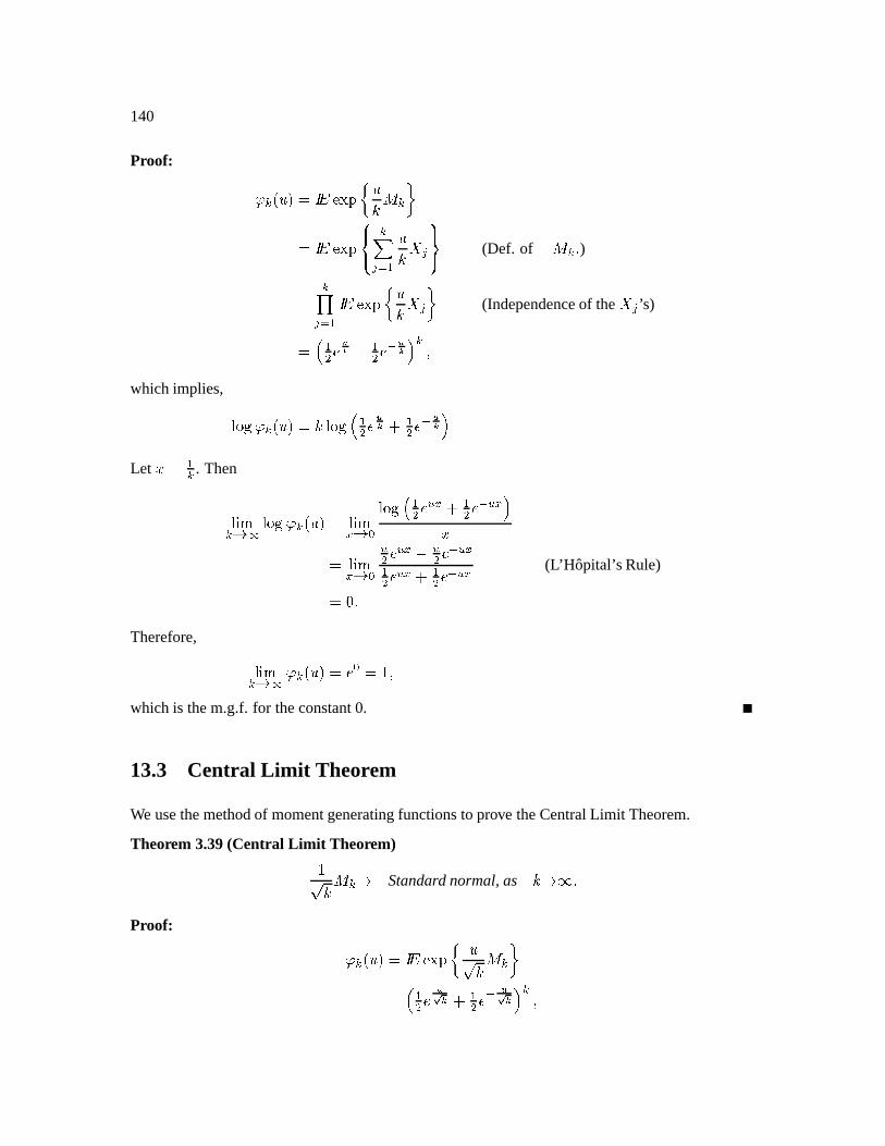
140
Proof: S ¾ ÍUijÎÊ?Ð ï ï÷ ÄÅ ñ ¾ Ê?Ð ï ï÷ ¾D ûBÔ ÄÅ ü "# (Def. ofñ ¾ Ï )Ê ¾T ûBÔ Ð ï ï÷ ÄÅ ü (Independenceof the ü ’s)Ê z ÔH VU W¬Á ÔH ô U W" ¾ Æ
which implies, 587:9 S ¾¿ÍUijÎÊ?Å 5B7"9az ÔH U W¬Á ÔH ô U W:Let J Ê Ô¾ . Then5 YX¾ r ; 587:9 S ¾¿ÍUijÎÊ 5 XZ r Ù 587:9½z ÔH \[ Z Á ÔH ô [ Z JÊ 5 XZ r Ù [ H [ Z Ë [ H ô [ ZÔH [ Z Á ÔH ô [ Z (L’Hopital’sRule)Ê?» ÏTherefore, 5 X¾ r ; S ¾¿ÍUijÎÊ6 Ù ÊòÀÆwhich is them.g.f. for theconstant0.
13.3 Central Limit Theorem
We usethemethodof momentgeneratingfunctionsto prove theCentralLimit Theorem.
Theorem 3.39(Central Limit Theorem)Àì Å ñ ¾r Standard normal,as År@ ÏProof: S ¾¿ÍUijÎÊ?Ð ï ï÷ Äì Å ñ ¾ Ê z ÔH U] W Á ÔH ô U] W ¾ Æ
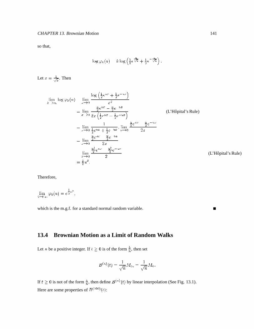
CHAPTER13. BrownianMotion 141
sothat, 587:9 S ¾¿ÍUijÎÊ?Å 5B7"9az ÔH U] W Á ÔH ô U] W ÏLet J Ê Ô^ ¾ . Then
5 X¾ r ; 587:9 S ¾dÍUÄrÎÊ 5 YXZ r Ù 587:9z ÔH [ Z Á ÔH ô [ Z J HÊ 5 YXZ r Ù [ H [ Z Ë [ H ô [ ZÛ J z ÔH [ Z Á ÔH ô [ Z (L’Hopital’sRule)Ê 5 YXZ r Ù ÀÔH [ Z Á ÔH ô [ Z Ï 5 XZ r Ù [ H [ Z Ë [ H ô [ ZÛ JÊ 5 YXZ r Ù [ H [ Z Ë [ H ô [ ZÛ JÊ 5 YXZ r Ù [ H 8[ Z Ë [ H ô [ ZÛ (L’Hopital’sRule)Ê ÔH Ä H ÏTherefore,
5 X¾ r ; S ¾¿ÍUijÎÊ6 ÔH [ Æwhich is them.g.f. for astandardnormalrandomvariable.
13.4 Brownian Motion asa Limit of RandomWalks
Let º beapositiveinteger. If _ < » is of theform ¾ú , thenset
= j ú m Í`_,ÎÊ Àì º ñba ú Ê Àì º ñ ¾ ÏIf _ < » is not of theform ¾ú , thendefine = j ú m Í`_OÎ by linearinterpolation(SeeFig. 13.1).
Herearesomepropertiesof = j Ô ÙIÙ m Í`_,Î :
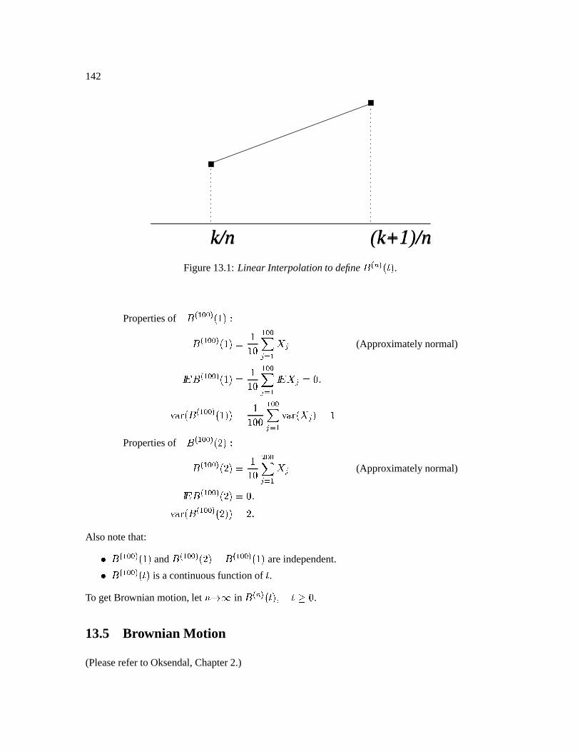
142
k/n (k+1)/nFigure13.1:Linear Interpolationto define= j ú m Íc_OÎ .
Propertiesof = j Ô ÙIÙ m Í,À8Î*p= j Ô ÙIÙ m Í,ÀÎ÷Ê ÀÀ» Ô ÙIÙD ûBÔ ü (Approximatelynormal)Ð ï[= j Ô ÙIÙ m Í,ÀÎ÷Ê ÀÀ» Ô ÙIÙD ûBÔ Ð ïü Ê?» Ï4 5 Í&= j Ô ÙIÙ m ÍþÀÎIÎ÷Ê ÀÀ»» Ô ÙIÙD û Ô 4 5 Íÿü ΣÊòÀPropertiesof = j Ô ÙIÙ m ÍUÛoÎ*p= j Ô ÙIÙ m ÍUÛÎ÷Ê ÀÀ» H ÙIÙD ûBÔ ü (Approximatelynormal)Ð ï[= j Ô ÙIÙ m ÍUÛÎ÷Ê?» Ï4 5 Í&= j Ô ÙIÙ m ÍpÛÎIÎ÷Ê?Û Ï
Also notethat:t = j Ô ÙIÙ m Í,À8Î and = j Ô ÙIÙ m ÍUÛoÎË6= j Ô ÙIÙ m ÍþÀÎ areindependent.t = j Ô ÙIÙ m Í`_,Î is acontinuousfunctionof _ .
To getBrownianmotion,let ºXr_ in = j ú m Í`_OÎmÆd_ < » .13.5 Brownian Motion
(Pleasereferto Oksendal,Chapter2.)
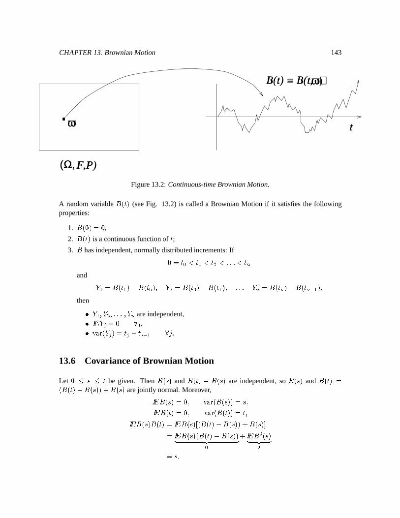
CHAPTER13. BrownianMotion 143
t
(Ω, F,P)
ω
B(t) = B(t,ω)
Figure13.2:Continuous-timeBrownianMotion.
A randomvariable =ÃÍ`_OÎ (seeFig. 13.2) is calleda Brownian Motion if it satisfiesthe followingproperties:
1. =ðÍU»ÎÊg» ,2. =ðÍ`_,Î is a continuousfunctionof _ ;3. = hasindependent,normallydistributedincrements:If»Ê)_ Ù ¼9_2Ôؼ9_¸H~¼ ÏÏ8Ï ¼9_ ú
and . ÔÊZ=ðÍ`_2Ô4ÎË6=ÃÍ`_ Ù Î&Æ .'HÊZ=ðÍ`_|H&ÎË6=ðÍc_IÔ4ÎmÆ ÏÏÏ . ú ÊZ=ÃÍ`_ ú ÎË6=ÃÍ`_ ú ôPÔÎ&Æthent . ÔÆL.XHÆ ÏÏ8Ï ÆL. ú areindependent,t Ð ï . Ê?» æÿdÆt 4 5 Í. ÎÊ)_ Ëe_ ôõÔ æÿ Ï
13.6 Covarianceof Brownian Motion
Let »?ÜgfÜg_ be given. Then =ÃÍ%fÎ and =ÃÍ`_OÎ0Ë%=ðÍhfÎ are independent,so =ÃÍ%fÎ and =ðÍ`_,ÎîÊÍ&=ÃÍ`_OÎË=ðÍ%f8ÎIÎ Ád=ÃÍ%fÎ arejointly normal.Moreover,Ð ï[=ðÍhfΣÊg»Æ 4 (5 Í&=ðÍhfÎIÎÊ6foÆÐ ï[=ðÍc_OΣÊg»Æ 4 (5 Í&=ðÍc_OÎIÎÊ)_ÆÐ ï[=ðÍ%f8ÎL=ðÍc_OΣÊgÐ ï[=ðÍ%f8Î&ÞëÍ&=ÃÍ`_OÎË6=ÃÍ%fÎ2Î Ád=ÃÍ%fÎ*ãÊgÐ ï[=ðÍ%f8ÎÍ&=ðÍc_OÎË=ðÍ%f8ÎIÎ Ù ÁÐ ï[= H ÍhfÎ iÊjf Ï
144
Thusfor any f < » , _ < » (not necessarilyfÜ9_ ), wehaveÐ ï =ÃÍ%fÎ =ðÍ`_,ΣÊ6flkm_ Ï13.7 Finite-DimensionalDistrib utions of Brownian Motion
Let » ¼9_2Ôؼ9_¸H~¼ ÏÏ8Ï ¼9_ úbegiven.Then Í&=ðÍ`_ Ô Î&Æ=ÃÍ`_ H Î&Æ ÏÏÏ Æ=ðÍ`_ ú Î2Îis jointly normalwith covariancematrix
LÊ nnn Ð ï = H Í`_IÔEÎ Ð ï[=ÃÍ`_IÔEÎL=ÃÍ`_¸H&Î ÏÏ8Ï Ð ï[=ðÍ`_2Ô4ÎL=ÃÍ`_ ú ÎÐ ï =ÃÍ`_ H ÎL=ðÍc_ Ô Î Ð ï[= H Í`_ H Î ÏÏ8Ï Ð ï[=ðÍ`_ H ÎL=ÃÍ`_ ú ÎÏÏ&Ï8Ï&ÏÏ&Ï8ÏÏ&ÏÏ&Ï8Ï&ÏÏ8Ï&ÏÏ&ÏÏ&Ï8Ï&ÏÏ8Ï&ÏÏ&ÏÏ&Ï8Ï&ÏÏ8Ï&ÏÏ&ÏÏ&Ï8ÏÏ&Ï8Ï&ÏÏ&ÏÏ&ÏÐ ï[=ðÍc_ ú ÎL=ÃÍ`_IÔ&ÎÐ ï =ÃÍ`_ ú ÎL=ÃÍ`_¸H&Î ÏÏ8Ï Ð ï[= H Í`_ ú Î1ooo
Ê nnn _IÔp_IÔ ÏÏ8Ï _IÔ_IÔp_¸H ÏÏ8Ï _¸HÏ&ÏÏ&Ï&Ï&Ï8Ï&Ï&ÏÏ&Ï&Ï8Ï&Ï&Ï_ Ô _ H ÏÏ8Ï _ ú1ooo
13.8 Filtration generatedby a Brownian MotionÒÇîÍ`_,ÎÖ a%q ÙRequiredproperties:t
For each_ , =ÃÍ`_OÎ is ÇîÍ`_,Î -measurable,t
For each_ andfor _¼9_2Ôؼ9_¸H~¼6rr3r¼9_ ú , theBrownianmotionincrements=ðÍ`_ Ô ÎË6=ðÍ`_,ÎÆ =ÃÍ`_ H ÎË6=ðÍc_ Ô ÎmÆ ÏÏÏ Æ =ðÍc_ ú ÎË6=ÃÍ`_ ú ôPÔ Îareindependentof ÇîÍ`_,Î .
Hereis oneway to constructÇîÍ`_OÎ . First fix _ . Let fç×ÞJ»Æ0_pã and óç3v0ÍUÐ ]0Î begiven.PutthesetÒ=ðÍ%f8Îç3·ÖØÊLÒmÓ p:=ðÍ%foÆ,ÓáÎç3ÝÖin ÇîÍ`_OÎ . Do this for all possiblenumbersf çÞJ» Æ0_Uã and ç@v ÍUÐ ]0Î . Thenput in every othersetrequiredby the -algebraproperties.
This ÇîÍ`_,Î containsexactly theinformationlearnedby observingtheBrownianmotionuptotime _ .ÒÇîÍ`_,ÎÖ a%q Ù is calledthefiltrationgeneratedby theBrownianmotion.
CHAPTER13. BrownianMotion 145
13.9 Martingale Property
Theorem 9.40 Brownianmotionis a martingale.
Proof: Let »·Ü/fÜ9_ begiven.ThenÐ ïÃÞ=ÃÍ`_OÎ8â ÇîÍ%fÎpãÊgÐ ïÃÞëÍ&=ðÍc_OÎ÷Ëæ=ÃÍ%fÎIÎBÁd=ðÍ%f8Îâ ÇîÍ%fÎOãÊgÐ ïÃÞ=ðÍ`_,Î÷Ëæ=ðÍhfÎ*ã Á@=ðÍ%f8ÎÊ,=ðÍ%f8Î ÏTheorem 9.41 Let C çîÐ ] begiven.Thené Í`_,Î£Ê ï÷ ø ËDC=ðÍc_OÎË ÔH C H _ ûis a martingale.
Proof: Let »·Ü/fÜ9_ begiven.ThenÐ ïÃÞ é Í`_OÎâ Ç Í%f8Î*ãPÊ?Ð ï ï÷ ÒdËDCÍ&=ðÍ`_,ΣË6=ÃÍ%fÎ÷Ád=ðÍhfÎIÎË ÔH C H ÍIÍ`_÷Ë:fÎ Á/fÎÖ ÇjÍhfÎ Ê?Ð ï é Í%f8Î ï÷ ÒdËDCÍ&=ðÍc_OÎËæ=ðÍhfÎIÎË ÔH C H Íc_|Ë:f8ÎÖ ÇîÍ%fÎ Ê é Í%fÎIÐ ï ü ï÷ ÒdËDCÍ&=ðÍc_OÎËæ=ðÍhfÎIÎË ÔH C H Í`_ Ë:f8ÎÖ ýÊ é Í%fÎ ï÷ ~ø ÔH ÍþËDCÎ H 4 5 Í&=ðÍ`_,ÎËæ=ÃÍ%fÎ2ÎË ÔH C H Í`_ ËsfÎûÊ é Í%fÎ Ï13.10 The Limit of a Binomial Model
Considerthe º ’ th Binomialmodelwith thefollowing parameters:t Ä ú Ê À£Á ^ ú Ï “Up” factor. ( ä=» ).t ½ ú ÊòÀË ^ ú Ï “Down” factor.t ÂØÊ?» .t ÈÉ ú Ê ÔIôt I[ I ôt I Ê õ ^ úH õ ^ ú Ê ÔH .t ÈÌ ú Ê ÔH .
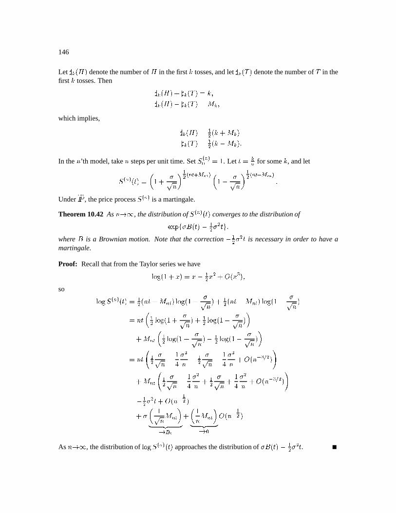
146
Let u2¾dÍUÕ Î denotethenumberof Õ in thefirst Å tosses,andlet uI¾¿ÍÿÚØÎ denotethenumberof Ú in thefirst Å tosses.Then uI¾¿ÍUÕ Î³Á.u2¾dÍÿÚØÎÊgÅõÆu ¾ ÍUÕ Î ËKu ¾ ÍÿÚØÎÊ ñ ¾ Æwhich implies, u ¾ ÍpÕ ÎÊ ÔH ÍpÅ0Á ñ ¾ Îu2¾dÍÿÚØÎÊ ÔH ÍpÅ Ë ñ ¾Î ÏIn the º ’ th model,take º stepsperunit time. Set ý j ú mÙ ÊòÀ . Let _Ê ¾ú for someÅ , andletý j ú m Í`_,Î£Ê `À£Á ì º b ÔH j ú a à > I,v m `ÀË ì º b ÔH j ú a ô > I,v m ÏUnder ; Ð Ñ , thepriceprocessý j ú m is amartingale.
Theorem 10.42 As º'r@ , thedistribution of ý j ú m Í`_,Î convergesto thedistributionofï÷ Ò< X=ðÍ`_,Î£Ë ÔH H _IÖdÆwhere = is a Brownianmotion. Notethat the correction Ë ÔH H _ is necessaryin order to haveamartingale.
Proof: Recallthatfrom theTaylorserieswehave587:9õÍ,À£Á J ÎÊ J Ë ÔH J H Á9w Í Jyx Î&Æso 587:9áý j ú m Í`_OÎÊ ÔH ÍUºV_ Á ñ ú a Î587:9õÍ,ÀÁ ì º ÎõÁ ÔH ÍUºV_Ë ñ ú a Î5B7"9PÍ,ÀË ì º ÎÊ?ºV_ ` ÔH 587:9PÍ,À£Á ì º ÎBÁ ÔH 587:9 Í,ÀË ì º Î bÁ ñ ú a ` ÔH 5B7"9PÍ,À£Á ì º Î Ë ÔH 587:9ÍþÀáË ì º Î bÊ?ºV_z ÔH ì º Ë À| Hº Ë ÔH ì º Ë À| Hº ÁswÍUº ô x õ H Î~Á ñ ú a z ÔH ì º Ë À| Hº Á ÔH ì º Á À| Hº ÁswÍUº ô x õ H Î~ÊòË ÔH H _PÁw ÍUº ô ÔH ÎÁd 2` Àì º ñ ú a b r v Á ` Àº ñ ú a b r Ù w ÍUº ô ÔH ÎAs ºXr_ , thedistributionof 5B7"9áý j ú m Í`_OÎ approachesthedistributionof X=ðÍ`_,Î£Ë ÔH H _ .
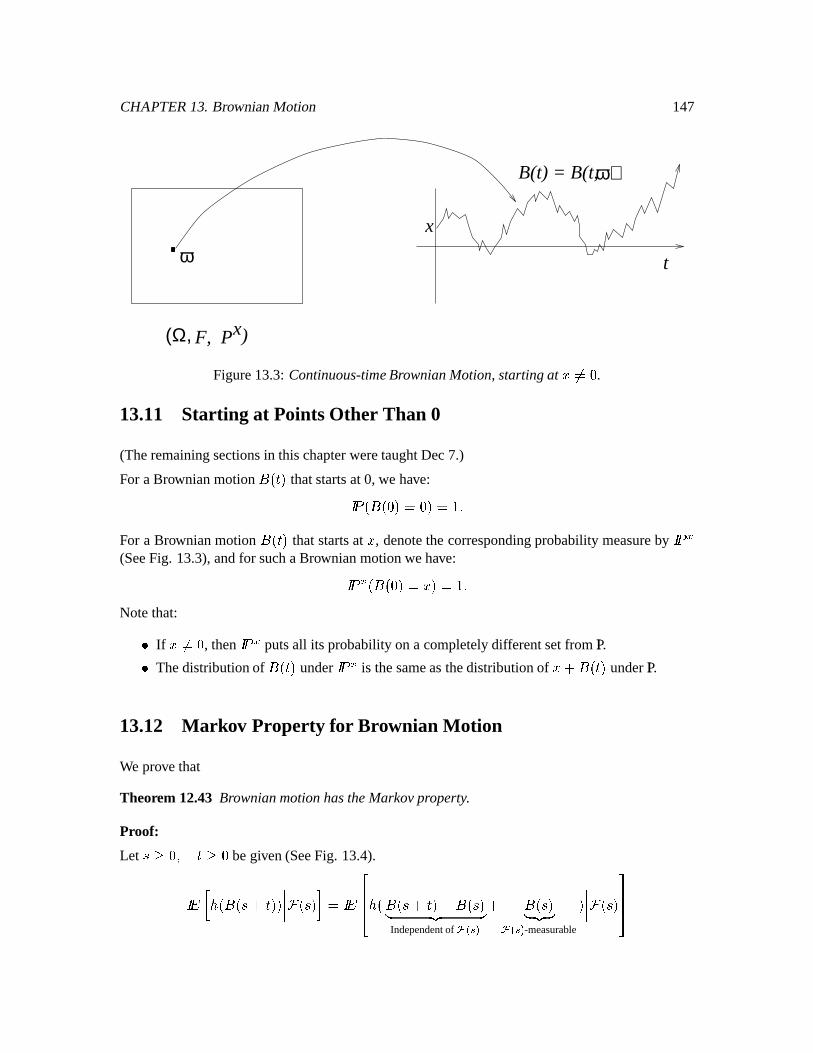
CHAPTER13. BrownianMotion 147
B(t) = B(t,ω)
tωx
(Ω, F, P )x
Figure13.3:Continuous-timeBrownianMotion,startingat b6 .13.11 Starting at Points Other Than 0
(Theremainingsectionsin thischapterweretaughtDec7.)
For aBrownianmotion =c thatstartsat0, we have: h= 6 A(For a Brownianmotion =c thatstartsat , denotethecorrespondingprobabilitymeasureby
(SeeFig. 13.3),andfor suchaBrownianmotionwehave: %= Notethat: If b6 , then
putsall its probabilityona completelydifferentsetfrom IP. Thedistributionof =c under
is thesameasthedistributionof 9=`~ underIP.
13.12 Mark ov Property for Brownian Motion
We prove that
Theorem 12.43 BrownianmotionhastheMarkovproperty.
Proof:
Let y begiven(SeeFig. 13.4). ` %=%ls~0 h ¡ (=%¢9~¤£:=%3¥ ¦¨§ ©Independentof ªl«¬® =%3¥ ¦¨§ ©ªl«¬® -measurable
%¯1°°±
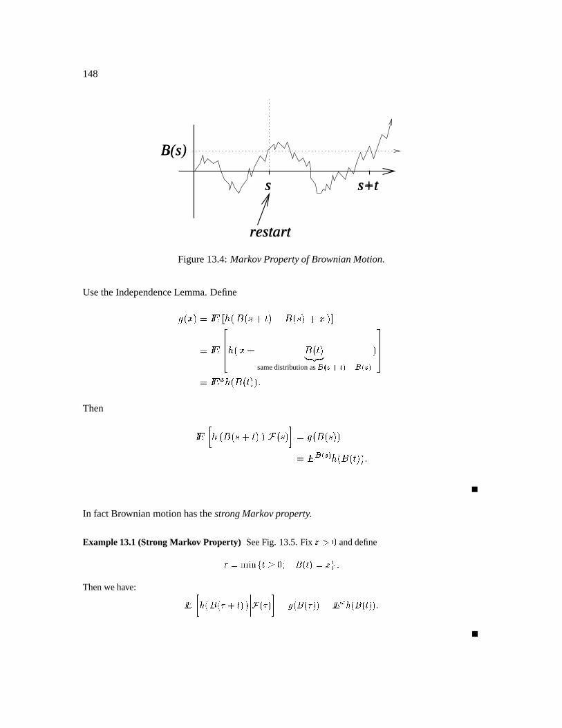
148
s s+t
restart
B(s)
Figure13.4:MarkovPropertyof BrownianMotion.
UsetheIndependenceLemma.Define² % /³1 =h´s¢£:=h/µ¶ ¡ · =c¥ ¦¨§ ©samedistribution as ¸´«¬¹º»(¼D¸¢«Y¬½ ¯ °°± %m`0
Then %m%lsV %3h¾ ² h=%30 ¸´«¬® %m`¿ In factBrownianmotionhasthestrongMarkovproperty.
Example13.1(Strong Mark ov Property) SeeFig. 13.5.Fix ÀÂÁQà anddefineÄ·Å:ÆÇFȤÉ~Ê¤Ë Ã(ÌÎÍ·Ï ÊÐÅ À ÑÓÒThenwehave: Ô Õ `Ö ÏÍ×Ï ÄlØÙÊÐÐ Ú Ï ÄÐ ¾ ÅeÛ Ï»Í·Ï ÄЮÐÜÅ
Ô ÕlÝ Ö Ï`Í·Ï ÊнРÒ
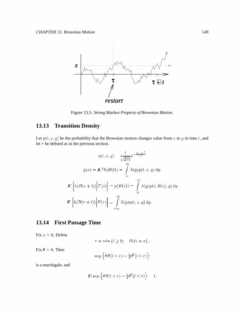
CHAPTER13. BrownianMotion 149
τ + t
restart
τ
x
Figure13.5:StrongMarkovPropertyof BrownianMotion.
13.13 Transition Density
Let Þc ,ß betheprobabilitythat theBrownianmotionchangesvaluefrom to ß in time , andlet à bedefinedasin theprevioussection.Þ` ,ß á âã +ä ¼lå1æ¿ç+è~éFêê®ë² % %=c0 ìí¼ ì ß %Þc ,ß î ß %m%´0 %3 ¾ ² %m%¿ ìí¼ ì ß %Þc m% ,ß î ß %m%às~0 hày ¾ ìí¼ ì ß %Þ` ,ß î ß13.14 First PassageTime
Fix ðï . Define à 6ñòóô õ =c ö Fix ÷ï . Then ø\ù!ú·û ÷+m`ýüðày¤£ÿþ ÷ c üðày is amartingale,and ø\ù!ú û ÷=`ýüðày £ÿþ ÷ ` üMày A
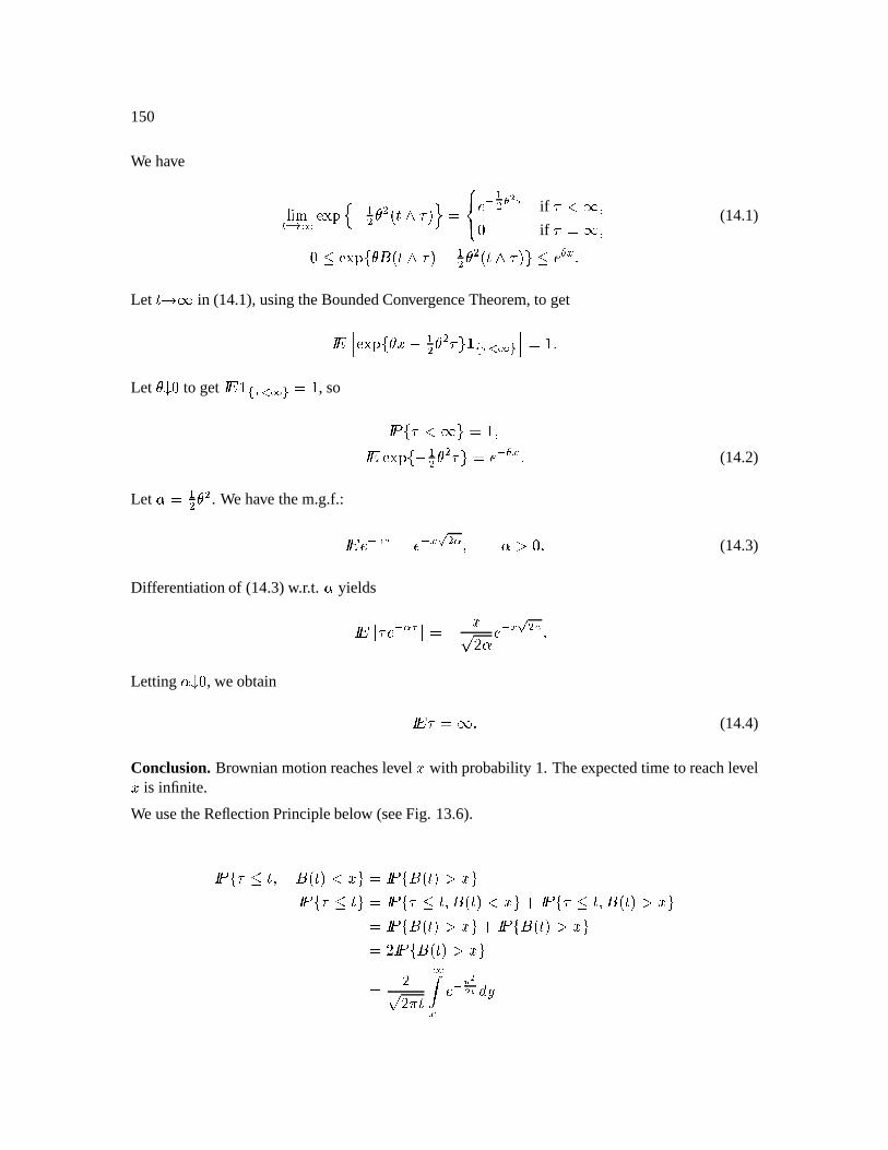
150
We have òYñº ì ø\ùyú û £mþ ÷ `ü ày ä ¼lþ ê if à if à (14.1) ø\ùyú ô ÷=`ýüMày¤£ þ ÷ ` üMày¨ö ä Let in (14.1),usingtheBoundedConvergenceTheorem,to get ø\ùyú ô ÷ £Aþ ÷ àVö ì ALet ÷ to get
ì A , so ô à /ö ø\ùyú ô £mþ ÷ àVö ä ¼ (14.2)
Let ! þ ÷ . We have them.g.f.: ä ¼#" ä ¼ %$ " !sï y (14.3)
Dif ferentiationof (14.3)w.r.t. ! yields£ '& à ä ¼(" ) £ á â ! ä ¼ %$ " Letting !* , weobtain à (14.4)
Conclusion.Brownianmotionreacheslevel with probability1. Theexpectedtime to reachlevel is infinite.
We usetheReflectionPrinciplebelow (seeFig. 13.6).
ô à m`+ .Óö ô m`ï.Óö ô à 0ö ô à m`, .öl ô à m` ï.ö ô m`ï.Óö ô m`ï.Óö â ô m` ï.ö âá âã ìí ä ¼ æ êê®ë î ß
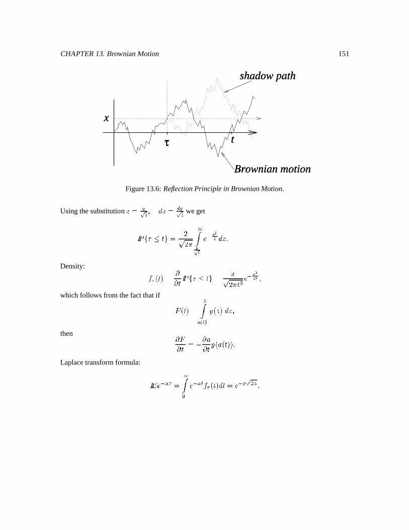
CHAPTER13. BrownianMotion 151
τ
x
shadow path
Brownian motion
t
Figure13.6:ReflectionPrinciple in BrownianMotion.
Usingthesubstitution - .$ º î/- 102.$ º weget ô à 0ö âá âã ìí è3 ë ä ¼54 êê î6- Density: 7 ` 988 ô à 0ö á âã ;: ä ¼ è êê®ë whichfollowsfrom thefact thatif < c =í> «Fº» ² ?-¤î6- then 8 <8 £ 8A@8 ² @ `¿ Laplacetransformformula: ä ¼(" ìí B ä ¼("º 7 c0î( ä ¼ %$ "

152
Chapter 14
The It o Integral
Thefollowing chaptersdealwith StochasticDifferentialEquationsin Finance. References:
1. B. Oksendal,StochasticDifferentialEquations, Springer-Verlag,1995
2. J.Hull, Options,FuturesandotherDerivativeSecurities,PrenticeHall, 1993.
14.1 Brownian Motion
(SeeFig. 13.3.) ?C ED is given,alwaysin thebackground,evenwhennot explicitly mentioned.Brownian motion, m` GF IH ³ 9KJLCM N , hasthefollowing properties:
1. = jyõ Technically, ô%F·õ = y2F j ö A ,
2. =`~ is a continuousfunctionof ,3. If B þ 63/ ;O , thentheincrements=` þ ¤£:=c B 3 =`;O¤£:=cPO ¼ þ
areindependent,normal,and m³ =cQ ¹ þ £K=cQh¶ 6y m³ =cQ ¹ þ Ü£K=cQ½¶ 2Q ¹ þ £e2Q 14.2 First Variation
Quadraticvariationis a measureof volatility. First we will considerfirst variation,
<R 7 , of afunction
7 `~ .153
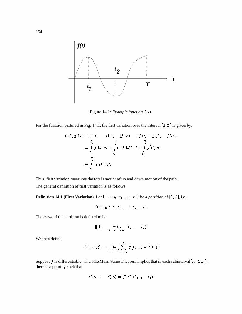
154
t
t
1
2t
f(t)
T
Figure14.1:Examplefunction
7 `~ .For thefunctionpicturedin Fig. 14.1,thefirst variationover theinterval
³ yES ¶ is givenby:<R*T B%U V#W 7 ³ 7 c þ ¤£ 7 ½¶£ ³ 7 c ¤£ 7 ` þ ½¶R ³ 7 S Ü£ 7 ` ½¶ º í B 7YX `~´î( º êíº ~£ 7YX `¿¤îVíº ê7(X `¢î
Ví B[Z 7YX c Z î( Thus,first variationmeasuresthetotalamountof upanddown motionof thepath.
Thegeneraldefinitionof first variationis asfollows:
Definition 14.1(First Variation) Let \ ÿô B þ 3y O ö bea partition of³ yES ¶ , i.e.,· B þ 63/ O ]Sµ
Themeshof thepartitionis definedto be
Z^Z \ Z^Z ñ_ ùQa` B%Ucbcbcb?U O ¼ þ ` Q ¹ þ £e Q We thendefine <R T B%U VdW 7 òñece fgece B O ¼ þhQa` B Z 7 cQ ¹ þ £ 7 cQ Z Suppose
7isdifferentiable.ThentheMeanValueTheoremimpliesthatin eachsubinterval
³ Q Q ¹ þ ¶ ,thereis apoint iQ suchthat 7 `2Q ¹ þ ¤£ 7 `Q 7 X ` iQ `2Q ¹ þ £:2Q
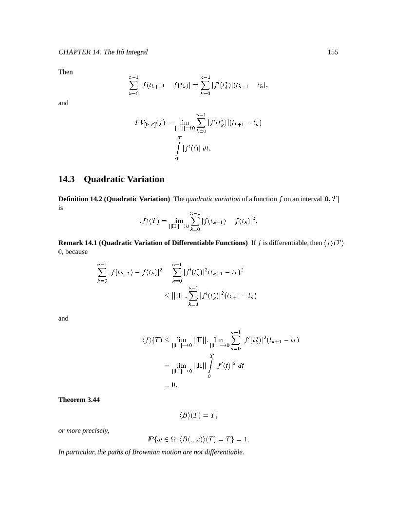
CHAPTER14. TheIto Integral 155
Then O ¼ þhQa` B Z 7 cQ ¹ þ £ 7 cQ Z O ¼ þhQj` B Z 7 X ` iQ Z `2Q ¹ þ £eQ and <R T B%U V#W 7 òñece fgece B O ¼ þhQa` B Z 7 X ` iQ Z `Q ¹ þ £bQ Ví BkZ 7YX c Z î( 14.3 Quadratic Variation
Definition 14.2(Quadratic Variation) Thequadraticvariationof afunction
7onaninterval
³ S ¶is l 7Am S òñece fnece B O ¼ þhQa` B Z 7 cQ ¹ þ ¤£ 7 `Q Z Remark 14.1(Quadratic Variation of DifferentiableFunctions) If
7isdifferentiable,then
l 7om S , because O ¼ þhQa` B Z 7 `Q ¹ þ ¤£ 7 `Q Z O ¼ þhQj` B Z 7YX c iQ Z cQ ¹ þ £eQ Z^Z \ Z^Z O ¼ þhQa` B Z 7 X c iQ Z cQ ¹ þ £eQand l 7Am S òñece fgece B Z^Z \ Z^Z òñece fgece B O ¼ þhQj` B Z 7 X ` iQ Z `Q ¹ þ £:Q òñece fgece B Z^Z \ Z^Z Ví B Z 7 X ` Z î(6yTheorem 3.44 l m S ]Sµor moreprecisely, ô%Fqp C õ l m GF m S rS ö AIn particular, thepathsof Brownianmotionarenot differentiable.
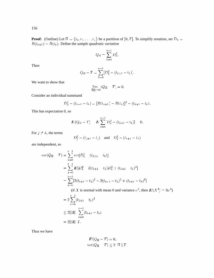
156
Proof: (Outline)Let \ Bô B þ 33y POVö bea partitionof³ yS ¶ . To simplify notation,set stQ =c Q ¹ þ ¤£:=c Q . Definethesamplequadratic variationu f O ¼ þhQa` B s Q
Then u f £ S) O ¼ þhQa` B ³ s Q £.`2Q ¹ þ £e2Q½¶ We wantto show that òñece fgece B u f £ S 6 Consideranindividualsummands Q £)`Q ¹ þ £:Q ³ =`2Q ¹ þ Ü£s=`2Q+¶ £)`Q ¹ þ £:2Q+ Thishasexpectation0, so u f £ S O ¼ þhQj` B ³ s Q £ ` Q ¹ þ £: Q ½¶ jyFor vðxw , theterms s y £.` y ¹ þ £e y and s Q £ ` Q ¹ þ £: Q areindependent,soz _ u f £ S O ¼ þhQa` B z _ ³ s Q £)`Q ¹ þ £:2Q½¶ O ¼ þhQa` B m³ st|Q £ â `Q ¹ þ £e2Q+Es Q 6`2Q ¹ þ £eQ ¶ O ¼ þhQa` B ³~ c Q ¹ þ £e Q £ â ` Q ¹ þ £: Q ÿ` Q ¹ þ £: Q ¶
(if is normalwith mean0 andvariance , then | | ) â O ¼ þhQa` B ` Q ¹ þ £e Q â ZZ \ ZZ O ¼ þhQj` B `Q ¹ þ £bQ â ZZ \ ZZ S
Thuswe have u f £ S jyz _ u f £ S â Z^Z \ Z^Z cS
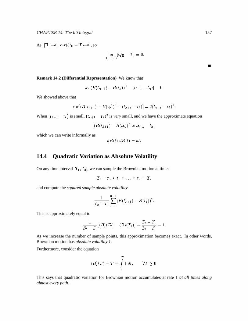
CHAPTER14. TheIto Integral 157
As Z^Z \ Z^Z , z _ u f £ S , so òñece fgece B u f £ S 6 Remark 14.2(Differential Representation) We know that =³ %=`2Q ¹ þ ¤£:m`Q0 £.`Q ¹ þ £eQ½¶ jyWe showedabove thatz _ ³ %=cQ ¹ þ £:=`2Q~ £.`Q ¹ þ £e2Q+¶ â `2Q ¹ þ £:2Q When ` Q ¹ þ £e Q is small, c Q ¹ þ £b Q is verysmall,andwehave theapproximateequation%m`Q ¹ þ Ü£Km`Q0 Q ¹ þ £eQ whichwe canwrite informally as î =`~´î =`~ î 14.4 Quadratic Variation asAbsoluteVolatility
Onany time interval³ S þ ES ¶ , we cansampletheBrownianmotionat timesS þ B þ 63/ PO ]S
andcomputethesquaredsampleabsolutevolatilityS £ S þ O ¼ þhQj` B %=cQ ¹ þ ¤£:=cQ0 This is approximatelyequaltoS £ S þ ³ l m S £ l m S þ ¶ S £ S þS £ S þ AAs we increasethe numberof samplepoints,this approximationbecomesexact. In otherwords,Brownianmotionhasabsolutevolatility 1.
Furthermore,considertheequationl m S ]S. Ví B î (S yThis saysthat quadraticvariation for Brownian motion accumulatesat rate 1 at all timesalongalmosteverypath.
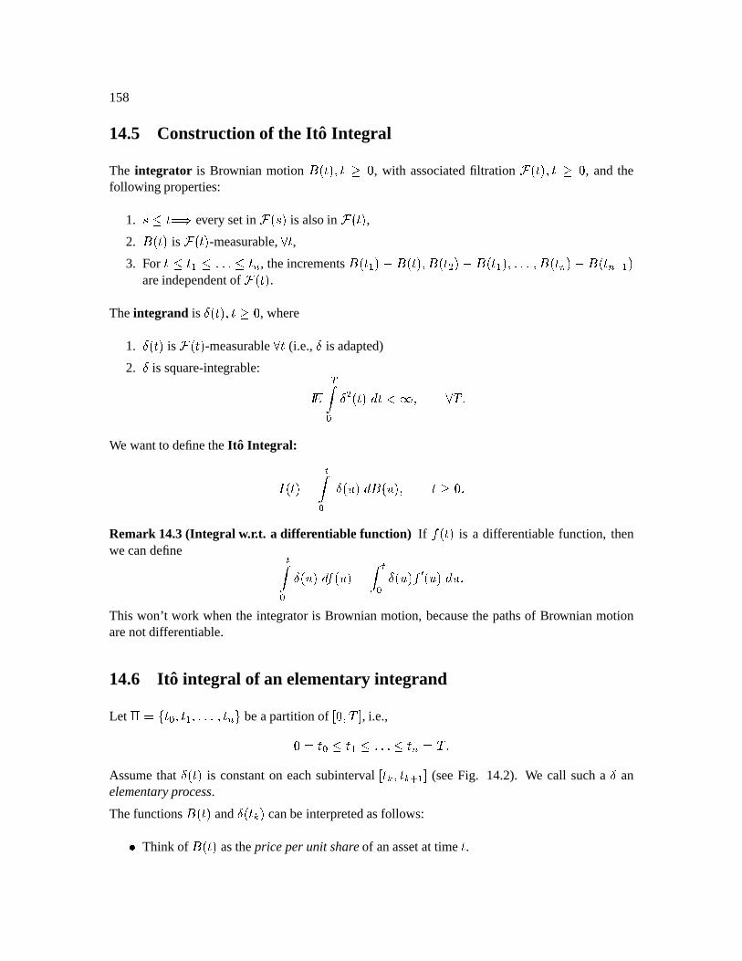
158
14.5 Construction of the It o Integral
The integrator is Brownian motion =`~ , with associatedfiltration c ? , andthefollowing properties:
1. A everysetin %3 is alsoin c ,2. =`~ is ` -measurable, ,3. For þ j6 PO , theincrementsm` þ £K=c =` ¤£Km` þ 3y m`PO ¤£Km`PO ¼ þ
areindependentof `~ .The integrand is !c ´ , where
1. !c is `~ -measurable (i.e., is adapted)
2. is square-integrable: Ví B `~´î(5 (SµWe wantto definetheIt o Integral: `~ ºí B y?V¤îRm? yRemark 14.3(Integral w.r.t. a differentiable function) If
7 `~ is a differentiablefunction, thenwecandefine ºí B y?V¤î 7 ? í ºB y?V 7YX ?V¤î/ This won’t work whenthe integratoris Brownianmotion, becausethe pathsof Brownianmotionarenotdifferentiable.
14.6 It o integral of an elementaryintegrand
Let \ ÿô B þ 3y O ö beapartitionof³ yES ¶ , i.e.,· B þ 63/ ;O ]Sµ
Assumethat y`~ is constanton eachsubinterval³ 2Q Q ¹ þ ¶ (seeFig. 14.2). We call sucha an
elementaryprocess.
Thefunctionsm` and !c Q canbeinterpretedasfollows: Think of m` asthepriceperunit shareof anassetat time .
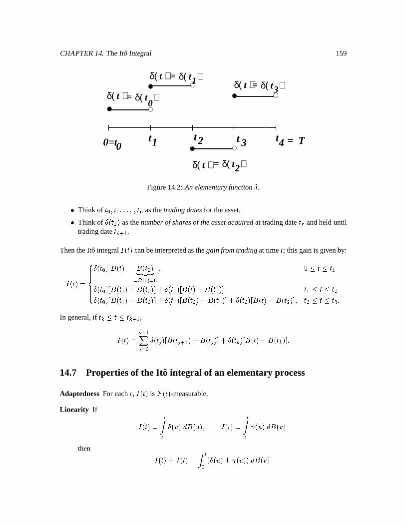
CHAPTER14. TheIto Integral 159
t )δ(
t )δ(δ( ) δ( t )=t
)tδ(
0=t0t t t = T2 3 4t1
0
δ( t )= 1
δ( t )= 2
δ( t )= 3
Figure14.2:Anelementaryfunction . Think of B þ 3V PO asthetradingdatesfor theasset. Think of !cQ asthenumberof sharesof theassetacquiredat tradingdate Q andhelduntiltradingdate2Q ¹ þ .
ThentheIto integral `~ canbeinterpretedasthegainfromtradingat time ; thisgainis givenby:
`~ y` B ³ =`~¤£ m` B ¥ ¦,§ ©` ¸´« B ` B ¶ t þy` B ³ =` þ ¤£s=` B ½¶!y` þ ³ =c¤£:m` þ ½¶ þ y` B ³ =` þ ¤£s=` B ½¶!y` þ ³ =c ¤£:m` þ ½¶R!c ³ m` £K=c ½¶ :
In general,if Q Q ¹ þ , `~ Q ¼ þhy ` B y` y ³ =` y ¹ þ £:=` y ½¶y!cQ ³ =`~¤£Km`Q½¶ 14.7 Propertiesof the It o integral of an elementaryprocess
AdaptednessFor each `~ is `~ -measurable.
Linearity If ` ºí B y?V¤îRm? c ºí B ?Vî =?Vthen `~ ` í ºB ?y?VA ?¿î =?V
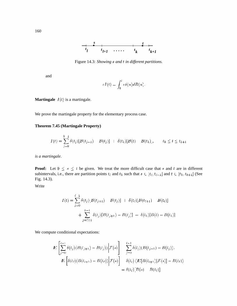
160
t tttl+1l k k+1
s t
. . . . .
Figure14.3:Showing and in differentpartitions.
and ` í ºB y?V0îRm? Martingale
` is a martingale.
We prove themartingalepropertyfor theelementaryprocesscase.
Theorem 7.45(Martingale Property) ` Q ¼ þhy ` B y` y ³ m` y ¹ þ ¤£:m` y ½¶ y`2Q+ ³ =`~¤£:=cQ½¶ Q Q ¹ þis a martingale.
Proof: Let r be given. We treat the moredifficult casethat and are in differentsubintervals,i.e., therearepartitionpoints ? and Q suchthat p ³ ? ¹ þ ¶ and p ³ Q Q ¹ þ ¶ (SeeFig. 14.3).
Write `~ ¼ þhy ` B y` y ³ m` y ¹ þ ¤£:=` y ¶ y` ³ m`? ¹ þ ¤£:m`?,½¶ Q ¼ þhy ` ¹ þ y` y ³ m` y ¹ þ ¤£:=c y ½¶ y`Q ³ =`~¤£:=`2Q½¶We computeconditionalexpectations: ¡ ¼ þhy ` B y` y 3%=` y ¹ þ Ü£s=` y 0 % ¯± ¼ þhy ` B y` y %m` y ¹ þ ¤£:=c y 0 y` %m` ¹ þ ¤£:m` %3½¾ !c m³ m` ¹ þ Z %h¶ £s=` 0 !c ³ m%¤£:m` ½¶
CHAPTER14. TheIto Integral 161
Thesefirst two termsaddup to %3 . Weshow thatthethird andfourth termsarezero. ¡ Q ¼ þhy ` ¹ þ y` y %m` y ¹ þ ¤£Km` y ~ %3 ¯± Q ¼ þhy ` ¹ þ ` y` y 3%=` y ¹ þ Ü£s=` y 0 ` y ¾ %3 ¾ Q ¼ þhy ` ¹ þ ¡ !c y Ü =³ =` y ¹ þ Z ` y ½¶£Km` y 0¥ ¦¨§ ©` B h ¯ °± y`2Q+3%=`~¤£:=cQ0 % ¾ ¡ y`2Q m³ m` Z `Q3½¶£K=cQ0¥ ¦,§ ©` B h ¯1°±
Theorem 7.46(It o Isometry) c í ºB ¤î6 Proof: To simplify notation,assume Q , so c Qhy ` B y` y ³ =` y ¹ þ ¤£s=` y ¥ ¦¨§ ©* ¶Eachs y hasexpectation0, anddifferent s y areindependent. `~ Qhy ` B y` y s yj
Qhy ` B ` y s y â h y y` y` y s s y
Sincethecrosstermshave expectationzero, `~ Qhy ` B m³ ` y s y ¶ Qhy ` B ` y %=` y ¹ þ ¤£s=` y ~ ` y ¾+¾ Qhy ` B ` y ` y ¹ þ £e y Qhy ` B º Píº ?V¤î/ í ºB ?V¤î/
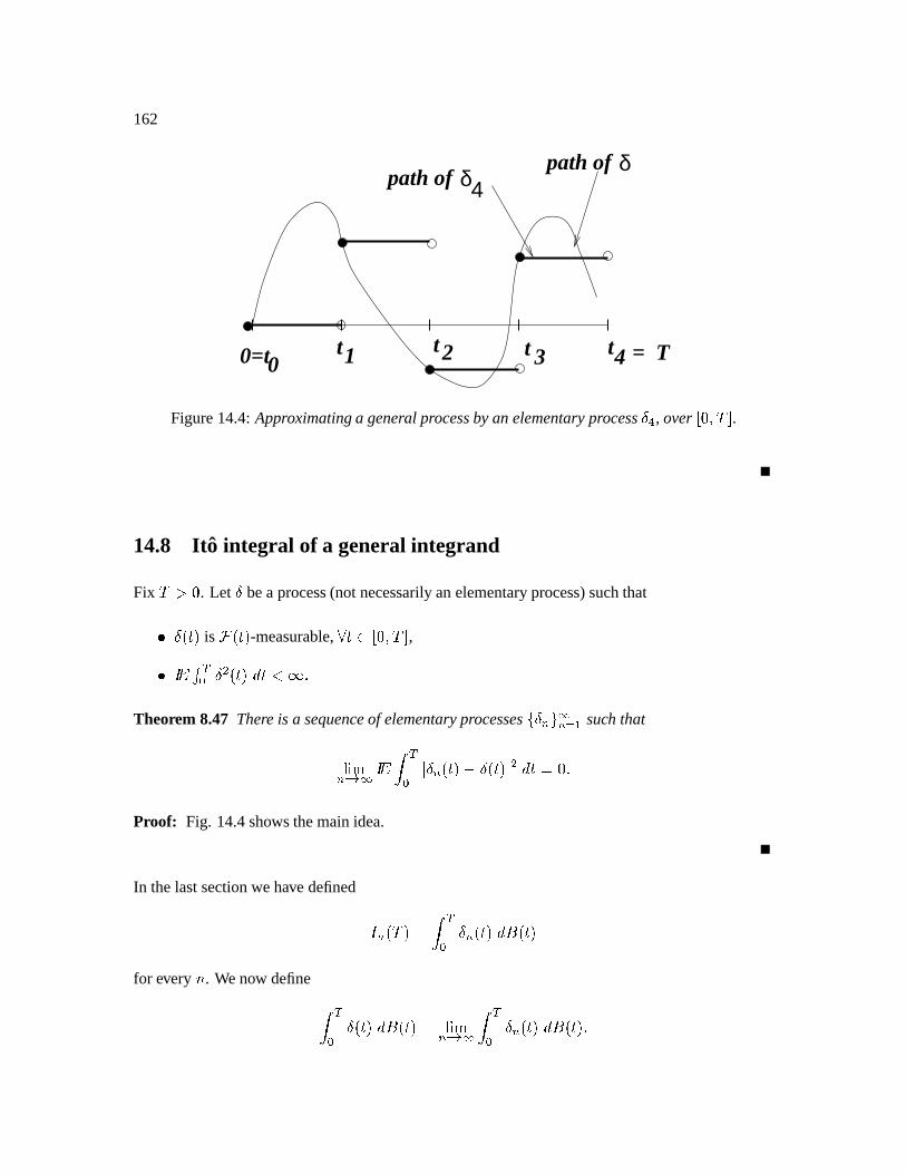
162
0=t0t t t = T2 3 4t1
path of path of
δδ4
Figure14.4:Approximatinga general processbyanelementaryprocess | , over³ yES ¶ .
14.8 It o integral of a generalintegrand
Fix S ï . Let bea process(not necessarilyanelementaryprocess)suchthat !c is `~ -measurable, p ³ yS ¶ , VB `~´î(5 Theorem 8.47 There is a sequenceof elementaryprocessesô aOyö ìO` þ such that òñO ì í VB Z aO c¤£!c Z î 6yProof: Fig. 14.4showsthemainidea.
In thelastsectionwehave defined Oý S í VB aOÓ`~¤îRm`for every . Wenow define í VB !c¤î =`~ òñO ì í VB aO `~´î =`~
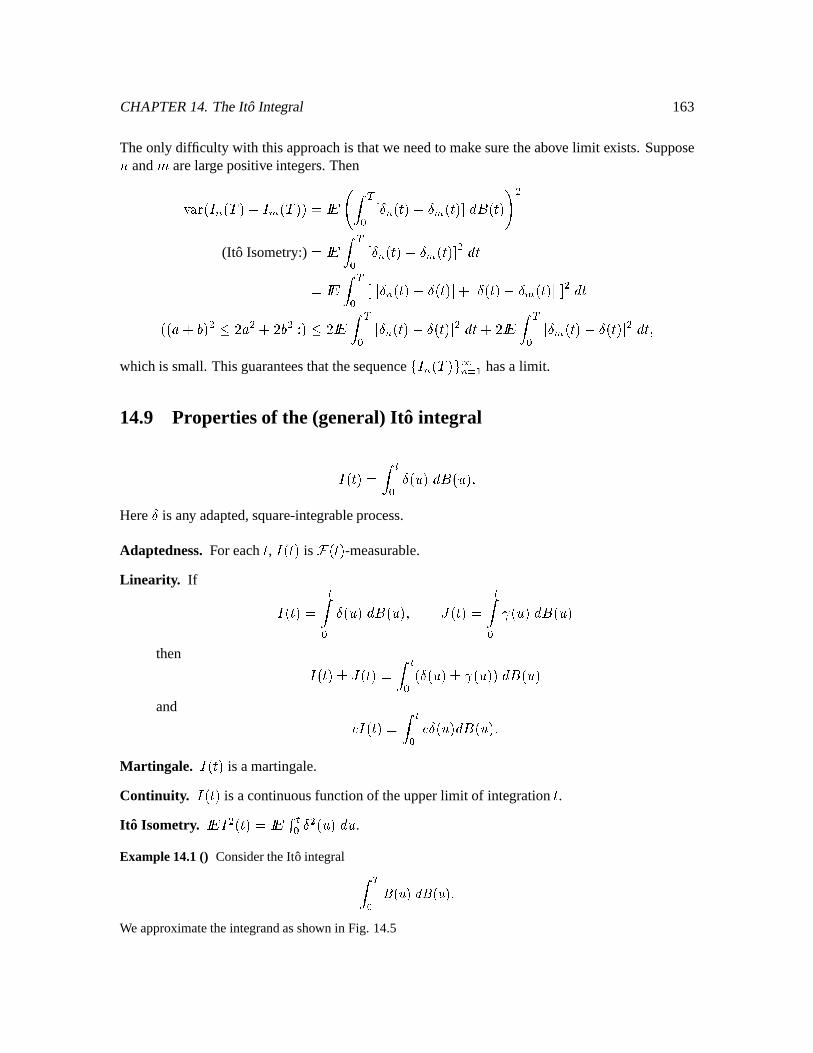
CHAPTER14. TheIto Integral 163
Theonly difficulty with thisapproachis thatwe needto makesuretheabove limit exists. Suppose and ¡ arelargepositiveintegers.Thenz _¢ Oý S Ü£ a£ S 0 ¤ í VB ³ aO ` £ £ `~½¶ î =`~2¥ (Ito Isometry:) í VB ³ aO ` £ £ `~½¶ î( í VB ³ Z aO ` £y` Z Z y`Ü£ £ ` Z ¶ î0 @ ¦\ â @ â ¦ H â í VB Z aO `~¤£§y` Z î( â í VB Z £ `¤£§y`~ Z î(
which is small.Thisguaranteesthatthesequenceô Oý S ¨ö ìO` þ hasa limit.
14.9 Propertiesof the (general)It o integral
` í ºB y?¤î = Here is any adapted,square-integrableprocess.
Adaptedness.For each , `~ is `~ -measurable.
Linearity . If ` ºí B y?V¤îRm? c ºí B ?Vî =?Vthen `~ ` í ºB ?y?VA ?¿î =?Vand ` í ºB y?V0îRm?
Martingale. `~ is amartingale.
Continuity. `~ is acontinuousfunctionof theupperlimit of integration .
It o Isometry. `~ ºB ¤î6 .
Example14.1() ConsidertheIto integral í©¨ª ͷϬ« РͷϬ« Ð ÒWe approximatetheintegrandasshown in Fig. 14.5
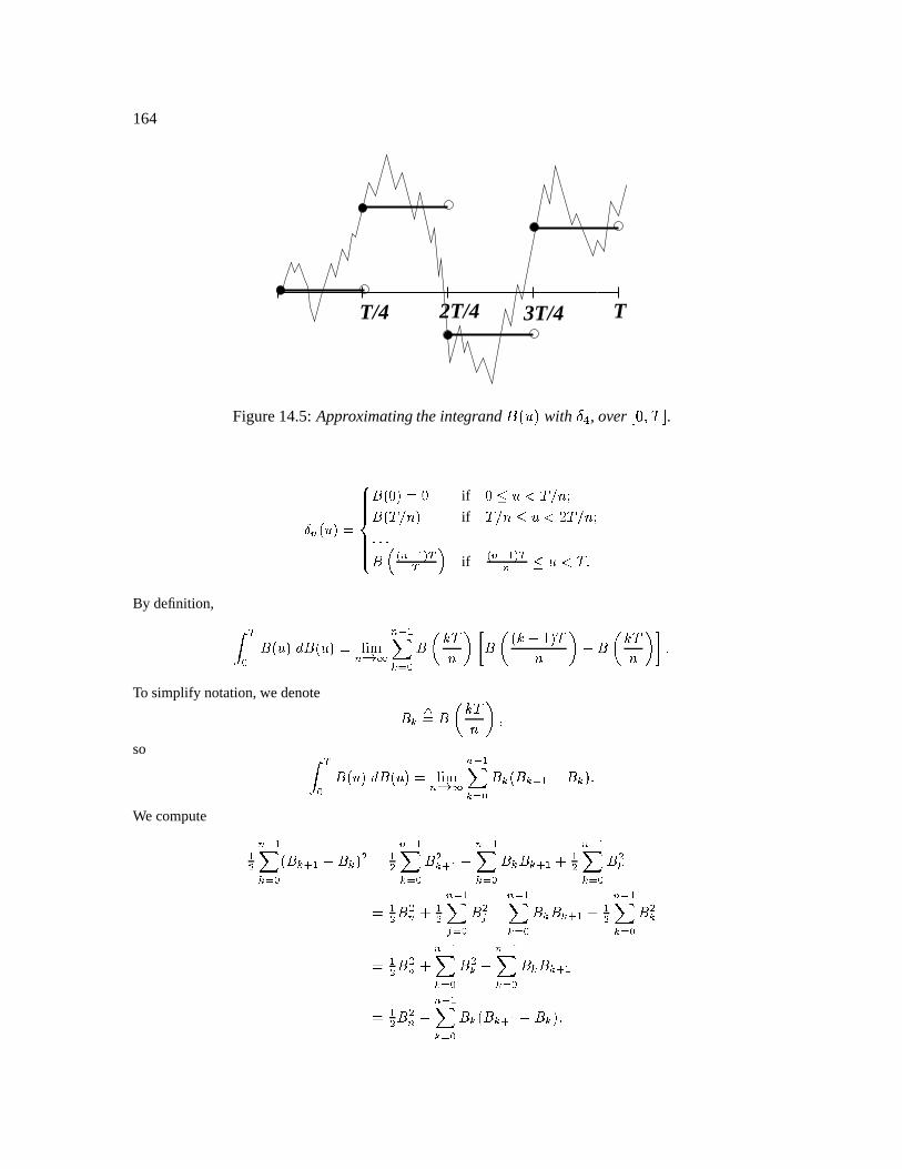
164
T/4 2T/4 3T/4 T
Figure14.5:Approximatingtheintegrand =?V with | , over³ yS ¶ .
®¯ Ï« ÐýŠͷϻà ÐýÅ Ã if Ã,°±«³²L´Kµ·¶ÌÍ·Ï^´Kµ·¶ Ð if ´Kµ·¶¸°§«³²§¹%´Kµ·¶ÌÒ,Ò¨Òͺd» ¯¼Y½¾ ¨¨ ¿ if » ¯¢¼(½P¾ ¨¯ °À«Á²Â´¤Ò
By definition, í¨ª Í·Ï« Ð Í·Ï« ÐýÅÄÃFÇFƯÅÇÆ ¯¼(½hÈ%É ª ÍrÊgË ´¶LÌ ÍrÊ Ï Ë ØͨР´¶ ÌÇÎ ÍrÊnË ´¶ÏÌ ¾ ÒTo simplify notation,wedenote Í ÈÐÅ ÍxÊË ´¶ ÌÇÑso íÒ¨ª Í×Ï« Ð Í·Ï« ÐýÅÃFÇFƯÅÂÆ ¯¢¼(½hÈÓÉ ª Í È Ï`Í È%Ô ½ Î Í È Ð ÒWe compute ½Õ ¯¼(½hÈ%É ª Ï»Í ÈÓÔ ½ Î Í È Ð Õ Å ½Õ ¯¢¼(½hÈ%É ª Í ÕÈÓÔ ½ Î ¯¢¼(½hÈÓÉ ª Í È Í È%Ô ½ Ø ½Õ ¯¢¼(½hÈÓÉ ª Í ÕÈÅ ½Õ Í Õ¯ Ø ½Õ ¯¼Y½hÖjÉ ª Í ÕÖ Î ¯¼Y½hÈÓÉ ª Í È Í È%Ô ½ Ø ½Õ ¯¼Y½hÈÓÉ ª Í ÕÈÅ ½Õ Í Õ¯ Ø ¯¢¼(½hÈÓÉ ª Í ÕÈ Î ¯¼(½hÈ%É ª Í È Í ÈÓÔ ½Å ½Õ Í Õ¯ Î ¯¢¼(½hÈÓÉ ª Í È Ï`Í È%Ô ½ Î Í È Ð Ò
CHAPTER14. TheIto Integral 165
Therefore, ¯¼(½hÈ%É ª Í È Ï»Í ÈÓÔ ½ Î Í È ÐýÅ ½Õ Í Õ¯ Î ½Õ ¯¼(½hÈ%É ª Ï»Í ÈÓÔ ½ Î Í È Ð Õ Ñor equivalently¯¼Y½hÈ%É ª ÍrÊgË ´¶§Ì ÍxÊ Ï Ë ØͨР´¶ ÌLÎ ÍxÊË ´¶§Ì ¾ Å ½Õ Í Õ Ï^´ Ð Î ½Õ ¯¢¼(½hÈÓÉ ª ÍrÊ Ï Ë ØÍ,Ð ´¶ Ì ÊIË´Ì ¾ Õ ÒLet ¶ ÅÇ×
andusethedefinitionof quadraticvariationto getíبª ͷϬ« РͷϬ« ÐOÅ ½Õ Í Õ Ï´ Ð Î ½Õ ´¤ÒRemark 14.4(Reasonfor the þ S term) If
7is differentiablewith
7 6 , thení VB 7 ?V¤î 7 ?V í VB 7 7YX ?¤î6 þ 7 ? VB þ 7 S
In contrast,for Brownianmotion,we haveí VB =?V0îRm? þ S ¤£ÿþ SµThe extra term þ S comesfrom thenonzeroquadraticvariationof Brownian motion. It hasto bethere,because í VB m?¢îRm? 6 (Ito integral is a martingale)
but þ S þ S14.10 Quadratic variation of an It o integral
Theorem 10.48(Quadratic variation of It o integral) Let ` í ºB y?¤î = Then l m `~ í ºB ?V¤î/
166
Thisholdsevenif is notanelementaryprocess.Thequadraticvariationformulasaysthatat eachtime , the instantaneousabsolutevolatility of
is ?V . This is the absolutevolatility of the
Brownianmotionscaledby thesizeof theposition(i.e. y` ) in theBrownianmotion. Informally,wecanwrite thequadraticvariationformulain differentialform asfollows:î `~¤î `~ `~¤î Comparethiswith î =`~´î =`~ î Proof: (For anelementaryprocess ). Let \ Bô B þ 3 POyö bethepartitionfor , i.e., y`~ y`Q3 for 2Q 2Q ¹ þ . To simplify notation,assume PO . We havel m ` O ¼ þhQa` B ³ l m `2Q ¹ þ Ü£ l m `2Q\½¶ Let uscompute
l m `Q ¹ þ £ l m `Q3 . Let Ù ÿô B þ 3y £ ö bea partitionQ B þ j¢ £ Q ¹ þ Then % y ¹ þ £ % y ¬ P í¬ y`Q3¤îRm? y`2Q ³ m% y ¹ þ ¤£Km% y ½¶ so l m cQ ¹ þ ¤£ l m `Q\ £ ¼ þhy ` B ³1 % y ¹ þ £ h y ½¶ `2Q £ ¼ þhy ` B ³ =h y ¹ þ ¤£:=% y ¶ Z^Z Ù Z^Z £V£y££y£6 `Q3`2Q ¹ þ £:2Q It followsthat l m ` O ¼ þhQj` B cQ`2Q ¹ þ £eQ O ¼ þhQj` B ºÚ
íº Ú ?¤î6Z^Z \ Z^Z £®£y£y£y£V£^ í ºB ¤î6
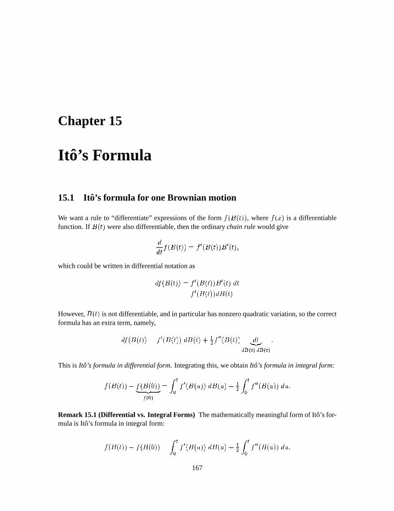
Chapter 15
It o’s Formula
15.1 It o’s formula for oneBrownian motion
We wanta rule to “dif ferentiate”expressionsof the form
7 %m`¿ , where
7 h is a differentiablefunction.If =`~ werealsodifferentiable,thentheordinarychain rule wouldgiveîî( 7 %m`¿ 7 X %=c00 X ` whichcouldbewritten in differentialnotationasî 7 h=`~0 7 X %m`0¿ X `¢î 7YX %m`0¿îRm`However, =`~ is notdifferentiable,andin particularhasnonzeroquadraticvariation,sothecorrectformulahasanextra term,namely,î 7 %=c0 7YX h=`~0¤îRm`ÜBþ 7YX X h=`~0 î¥,¦¨§¨©0 ¸¢« º» 0 ¸´«Fº» This is Ito’s formulain differential form. Integratingthis,weobtainIto’s formulain integral form:7 %=`~0¤£ 7 %m 0¥ ¦,§ ©Û « B í ºB 7YX %=?V0¤î =?VýBþ í ºB 7YXcX %m?0¤î6 Remark 15.1(Differential vs. Integral Forms) Themathematicallymeaningfulform of Ito’sfor-mulais Ito’s formulain integral form:7 %=`~0¤£ 7 %m 0 í ºB 7YX %=?V0¤î =?VýBþ í ºB 7YXcX %m?0¤î6
167
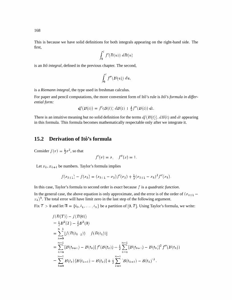
168
This is becausewe have solid definitionsfor both integralsappearingon the right-handside. Thefirst, í ºB 7 X %=0¢îRm?is anIto integral, definedin thepreviouschapter. Thesecond,í ºB 7(X X %=0¤î6 is aRiemannintegral, thetypeusedin freshmancalculus.
For paperandpencilcomputations,themoreconvenientform of Ito’s rule is Ito’s formulain differ-ential form: î 7 %m`0 7 X %=`~0¤î =`~ý þ 7 XcX %=`~0¤î( Thereis anintuitivemeaningbut nosoliddefinitionfor thetermsî 7 %m`¿ î =`~ and î( appearingin this formula.This formulabecomesmathematicallyrespectableonly afterwe integrateit.
15.2 Derivation of It o’s formula
Consider
7 % þ , sothat 7YX %V 7YXcX % Let (Q YQ ¹ þ benumbers.Taylor’s formulaimplies7 %(Q ¹ þ ¤£ 7 %(Q h(Q ¹ þ £:YQ 7YX %YQýBþ h(Q ¹ þ £s(Q3 7YXcX %YQ
In thiscase,Taylor’s formulato secondorderis exactbecause
7is aquadratic function.
In thegeneralcase,theaboveequationis only approximate,andtheerroris of theorderof %(Q ¹ þ £ Q : . Thetotalerrorwill have limit zeroin thelaststepof thefollowing argument.
Fix S ï andlet \ ÿô B þ 3V ;Oyö bea partitionof³ yS ¶ . UsingTaylor’s formula,wewrite:7 %m S 0¤£ 7 %m 0 þ S £ þ O ¼ þhQa` B ³ 7 %m`Q ¹ þ 0Ü£ 7 h=`2Q+¿½¶ O ¼ þhQa` B ³ m`Q ¹ þ ¤£:m`Q½¶ 7YX %m`Q0 þ O ¼ þhQj` B ³ m`Q ¹ þ ¤£:m`Q½¶ 7YXcX h=`2Q+¿ O ¼ þhQa` B m`Q ³ m`Q ¹ þ ¤£s=`2Q+¶( þ O ¼ þhQa` B ³ =`2Q ¹ þ £:=`2Q+¶
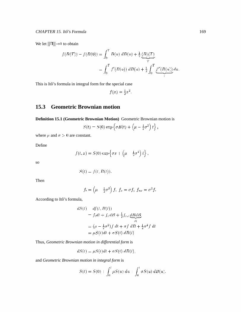
CHAPTER15. Ito’sFormula 169
We let Z^Z \ Z^Z to obtain7 %m S 0¤£ 7 %m 0 í VB m?¢îRm?OBþ l m S ¥ ¦¨§ ©V í VB 7YX %m?0¤î =ýBþ í VB 7YXcX %m?¿¥ ¦¨§ ©þ î/ This is Ito’s formulain integral form for thespecialcase7 % þ 15.3 GeometricBrownian motion
Definition 15.1(GeometricBrownian Motion) GeometricBrownianmotionisÜ ` Ü ø\ù!ú û O=`~ÝºÞ £Aþ ¿ whereÞ and eï areconstant.
Define 7 c V Ü ø\ùyú û OÝºÞ £Aþ ¿ so Ü `~ 7 ` =`~0 Then 7 º º Þ £Aþ ¿ 7 7 7 7 \ 7 Accordingto Ito’s formula,î Ü ` î 7 ` m`0 7 º î 7 îR/ þ 7 \ îRîR¥ ¦¨§ ©0 º ¬Þ £ þ 7 î( 7 î ) þ 7 î Þ Ü `~0î( Ü `¤î =`~Thus,GeometricBrownianmotionin differential form isî Ü ` Þ Ü `~0î( Ü `¤î =`~ andGeometricBrownianmotionin integral form isÜ `~ Ü í ºB Þ Ü ¤î6 í ºB Ü ?Vî =
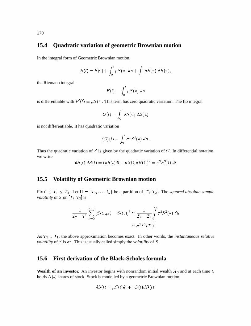
170
15.4 Quadratic variation of geometricBrownian motion
In theintegral form of GeometricBrownianmotion,Ü ` Ü V í ºB Þ Ü ?V¤î/· í ºB Ü ¤î =?V theRiemannintegral < `~ í ºB Þ Ü ?V¤î/is differentiablewith
< X c Þ Ü ` . This termhaszeroquadraticvariation.TheIto integralß `~ í ºB Ü ?Vî =is notdifferentiable.It hasquadraticvariationl ß m c í ºB Ü ?¤î6 Thusthequadraticvariationof
Üis givenby thequadraticvariationof
ß. In differentialnotation,
wewrite î Ü `~¤î Ü ` ¬Þ Ü c0î( Ü `¿îRm`0 Ü c¤î(15.5 Volatility of GeometricBrownian motion
Fix L'S þ 'S . Let \ ô B 33 ;Oyö bea partitionof³ S þ S ¶ . Thesquaredabsolutesample
volatility ofÜ
on³ S þ S ¶ isS £ S þ O ¼ þhQj` B ³ Ü `Q ¹ þ ¤£ Ü `2Q½¶ S £ S þ V êíV Ü ¤î6 Ü S þ
As S S þ , the above approximationbecomesexact. In otherwords,the instantaneousrelativevolatility of
Üis . This is usuallycalledsimply thevolatility of
Ü.
15.6 First derivation of the Black-Scholesformula
Wealth of an investor. An investorbeginswith nonrandominitial wealth B andat eachtime ,holds àð`~ sharesof stock.Stockis modelledby a geometricBrownianmotion:î Ü ` Þ Ü c0î( Ü `¿îRm`
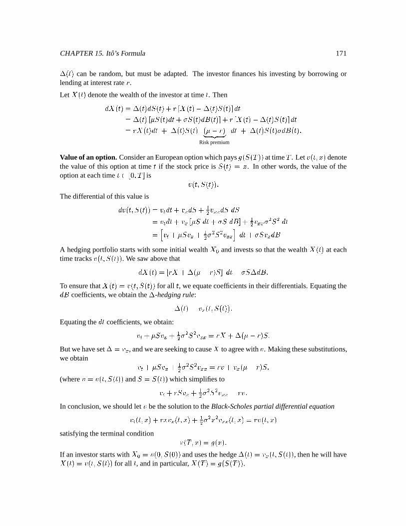
CHAPTER15. Ito’sFormula 171àð`~ can be random,but mustbe adapted.The investorfinanceshis investingby borrowing orlendingat interestrate á .Let .` denotethewealthof theinvestorat time . Thenî¢.` àð`~0î Ü `~ á ³ .`~£àð`~ Ü `~½¶î àð`~ ³ Þ Ü `~0î( Ü `0î =c½¶Rá ³ .`¤£§àM` Ü `¶8î( á .`0î(=àM` Ü ` ¬Þ £§á¥ ¦,§ ©
Riskpremium
î àðc Ü `VîRm` Valueof an option. ConsideranEuropeanoptionwhichpays² Ü S 0 attime S . Let â` denotethe valueof this option at time if the stockprice is
Ü `~ . In otherwords,the valueof theoptionateachtime p ³ yS ¶ is â` Ü `~0 Thedifferentialof thisvalueisî/â` Ü c0 â º î( â î Ü Bþ â \ î Ü î Ü â º î( â ³ Þ Ü î(ý Ü î ¶!Bþ â \ Ü î( â º Þ Ü â þ Ü â \ îý Ü â î A hedgingportfolio startswith someinitial wealth B andinvestssothat thewealth .` at eachtime tracks â c Ü `¿ . We saw abovethatî¢.` ³ á àM¬Þ £á Ü ¶µî( Ü àî To ensurethat .` â` Ü c0 for all , weequatecoefficientsin theirdifferentials.Equatingtheî coefficients,weobtainthe à -hedgingrule:àð` â ` Ü `~0 Equatingthe î coefficients,weobtain:â º Þ Ü â þ Ü â \ á àð¬Þ £§á Ü But wehaveset à â , andweareseekingto cause to agreewith â . Makingthesesubstitutions,weobtain â º Þ Ü â Bþ Ü â \ áâDâ ¬Þ £§á Ü (where â â c Ü `¿ and
Ü Ü `~ ) whichsimplifiestoâ º á Ü â þ Ü â \ áâ In conclusion,weshouldlet â bethesolutionto theBlack-Scholespartial differentialequationâ º c Vá+Yâ c V þ â \ ` áâ` satisfyingtheterminalcondition â Sµ ² %V If aninvestorstartswith B â y Ü 0 andusesthehedgeàð`~ â ` Ü `~0 , thenhewill have.` â ` Ü `0 for all , andin particular, . S ² Ü S ¿ .
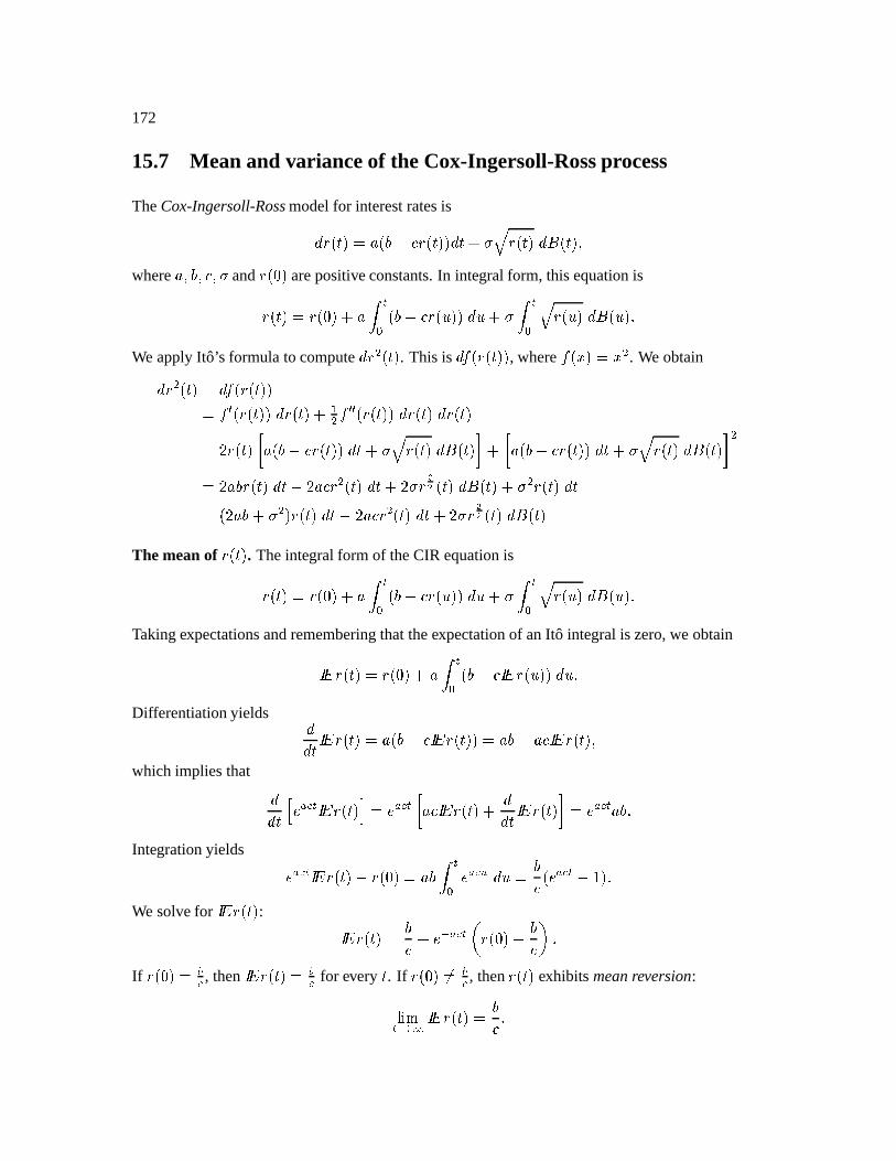
172
15.7 Mean and varianceof the Cox-Ingersoll-Rossprocess
TheCox-Ingersoll-Rossmodelfor interestratesisî/áy`~ @ ¦l£ á!c00î(Kã áy`¤î =c where@ ¦ and áy arepositiveconstants.In integral form, thisequationisáy` á! @ í ºB ?¦¢£ áy?V0Üî/· í ºB ã á!¤î =?V We applyIto’s formulato computeî6á `~ . This is î 7 ?áy`0 , where
7 h . We obtainî6á c î 7 á!c0 7YX ?áy`¿¤î/áy`~ Bþ 7(XcX ?áy`¿¤î/áy`~¤î/áy`~ â áy`~ @ ?¦¢£ áy`~0Üînã á!c¤î =`~ ¾ @ ¦´£ áy`~0¤înã áy`¤î =`~ ¾ â @ ¦%áy`¤î(£ â @ á `¢î â áYäê `¤î =`~ý áy`~¤î â @ ¦Ü áy`~¤îÜ£ â @ á `¢î â áYäê `¤î =cThe meanof á!c . Theintegral form of theCIR equationisáy` á! @ í ºB ?¦¢£ áy?V0Üî/· í ºB ã á!¤î =?V Takingexpectationsandrememberingthattheexpectationof anIto integral is zero,we obtain áy`~ áy @ í ºB ?¦¢£ áy?0Üî6 Differentiationyields îî áy` @ ?¦l£ áy`~0 @ ¦l£ @ áy` which impliesthat îî( ä >jå º áy`~ ä >jå º @ á!c îî( áy`~ ¾ ä >jå º @ ¦ Integrationyields ä >aå º áy`Ü£áy @ ¦ í ºB ä >jå¬æ î/ ¦ ä >aå º £ We solvefor
áy` : áy` ¦ ä ¼ >jå º Ê áy Ü£ ¦ Ì If áy =å , then
áy` = å for every . If áy =å , then áy`~ exhibits meanreversion: òñº ì áy` ¦
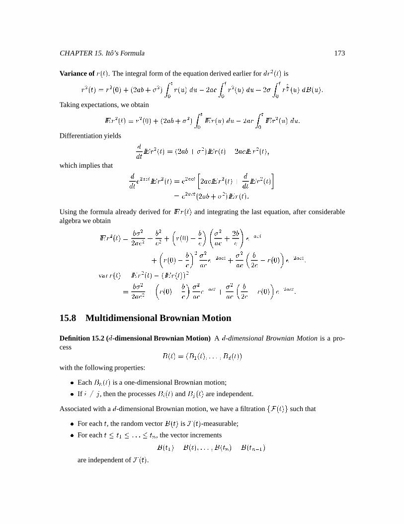
CHAPTER15. Ito’sFormula 173
Varianceof áy`~ . Theintegral form of theequationderivedearlierfor î6á `~ isá `~ á ý6 â @ ¦ í ºB áy?V¤î/ £ â @ í ºB á ?V¤î/ â í ºB á(äê ?¤î =?V Takingexpectations,weobtain á `~ á â @ ¦Ü í ºB áy?Üî/ £ â @ í ºB á ¤î6 Differentiationyields îî( á ` â @ ¦ áy`O£ â @ á ` which impliesthat îî( ä >jå º á ` ä >aå º â @ á c îî( á ` ¾ ä >aå º â @ ¦ áy`~ Using the formula alreadyderived for
áy` andintegratingthe last equation,after considerablealgebraweobtain á c ¦% â @ ¦ Ê áy Ü£ ¦ Ì ¤ @ â ¦ ¥ ä ¼ >aå º Ê áy £ ¦ Ì @ ä ¼ >jå º @ Ê ¦â £áy Ì ä ¼ >jå º z _¢ á!c á `¤£) áy`¿ ¦% â @ Ê áy Ü£ ¦ Ì @ ä ¼ >jå º @ Ê ¦â £§áy Ì ä ¼ >aå º 15.8 Multidimensional Brownian Motion
Definition 15.2( î -dimensionalBrownian Motion) A î -dimensionalBrownianMotion is a pro-cess =`~ h þ `~ 3y 0 `~0with thefollowing properties: Each+Qy` is a one-dimensionalBrownianmotion; If ç v , thentheprocesses c and y ` areindependent.
Associatedwith a î -dimensionalBrownianmotion,wehave afiltration ô ` ö suchthat For each , therandomvector m` is c -measurable; For each þ 636 O , thevectorincrements=` þ Ü£Km` 33 m`PO ¤£Km`PO ¼ þ areindependentof `~ .
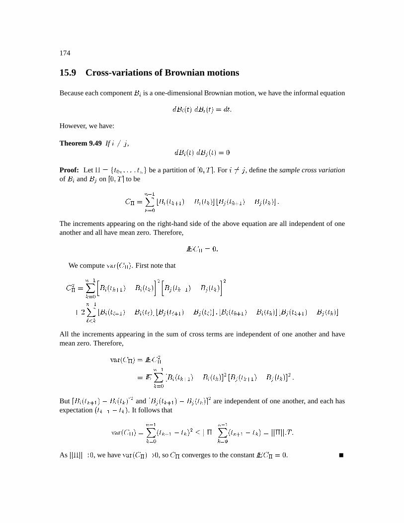
174
15.9 Cross-variations of Brownian motions
Becauseeachcomponent is aone-dimensionalBrownianmotion,wehavetheinformalequationî `~´î ` î However, wehave:
Theorem 9.49 If çl v , î `~´î y ` 6Proof: Let \ Aô B 3V PO ö bea partitionof
³ yES ¶ . For ç v , definethesamplecrossvariationof and y on
³ yES ¶ to beè f O ¼ þhQa` B ³ `Q ¹ þ ¤£: `Q3½¶ ³ y `2Q ¹ þ ¤£: y `Q½¶ Theincrementsappearingon theright-handsideof theabove equationareall independentof oneanotherandall have meanzero.Therefore, è f 6y
We computez _ è f . First notethatè f O ¼ þhQj` B `2Q ¹ þ Ü£s `Q ¾ y `Q ¹ þ ¤£K y `2Q ¾ â O ¼ þh Q ³ ` ¹ þ ¤£: ` ¶ ³ y ` ¹ þ ¤£K y ` ¶ ³ `2Q ¹ þ £: `2Q½¶ ³ y cQ ¹ þ ¤£: y `2Q½¶
All the incrementsappearingin the sumof crosstermsare independentof oneanotherandhavemeanzero.Therefore,z _¢ è f è f O ¼ þhQa` B ³ `Q ¹ þ ¤£K `Q½¶ ³ y `Q ¹ þ ¤£: y `Q3½¶ But
³ `2Q ¹ þ Ü£s `Q½¶ and³ y `2Q ¹ þ £: y `Q3½¶ areindependentof oneanother, andeachhas
expectation`2Q ¹ þ £e2Q . It followsthatz _ è f O ¼ þhQa` B cQ ¹ þ £eQ Z^Z \ Z^Z O ¼ þhQa` B `Q ¹ þ £:2Q+ Z^Z \ Z^Z cSAs Z^Z \ Z^Z , we have z _ è f , so
è f convergesto theconstant è f 6 .
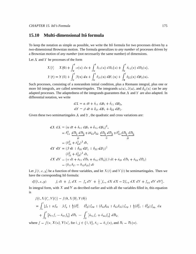
CHAPTER15. Ito’sFormula 175
15.10 Multi-dimensional It o formula
To keepthenotationassimpleaspossible,we write the Ito formulafor two processesdrivenby atwo-dimensionalBrownianmotion. Theformulageneralizesto anynumberof processesdrivenbya Brownianmotionof anynumber(notnecessarilythesamenumber)of dimensions.
Let and é beprocessesof theform.` . í ºB !?V´î6· í ºB þ0þ ?¤î þ ý í ºB þ ?V¤îR éð`~ é? ý í ºBÇê ?¤î6 í ºB þ ?V¤îR þ ?V í ºB ?V¤îR ?V Suchprocesses,consistingof a nonrandominitial condition,plusa Riemannintegral, plusoneormoreIto integrals,arecalledsemimartingales. The integrands!l? ê ?V and y ?V canbeanyadaptedprocesses.Theadaptednessof theintegrandsguaranteesthat and é arealsoadapted.Indifferentialnotation,wewrite î¢ !eî( þ¿þ î þ þ îR îYé ê î þ î þ E î Giventhesetwo semimartingales and é , thequadraticandcrossvariationsare:
î¢ î ?!Mî þ0þ î þ þ îR þ0þ î þ î þ¥ ¦¨§ ©0 º â þ0þ þ î þ î ¥ ¦¨§ ©B þ î îR ¥ ¦,§ ©0 º ? þ¿þ þ î( î(éÿî(é ê î( þ îR þ î ? þ î( î î(é ?!Mî þ0þ î þ þ îR ê î(Ó þ î þ î ? þ¿þ þ þ ¤î(Let
7 ` ¨ß bea functionof threevariables,andlet c and éð`~ besemimartingales.Thenwehave thecorrespondingIto formula:î 7 ` ¨ß 7 º î(= 7 î¢ 7 . îYé þ ³ 7 \ î î â 7 . î¢ îYé 7 .. îYé îYé·¶ In integral form, with and é asdecribedearlierandwith all thevariablesfilled in, thisequationis 7 ` .` éÂc0Ü£ 7 . é 0 í ºB ³ 7 º ! 7 ê 7 . Bþ ? þ0þ þ 7 \ þ0þ þ þ 7 . Bþ ? þ 7 .E. ¶Óî6 í ºB ³ þ0þ 7 þ 7 . ¶ î þ í ºB ³ þ 7 7 . ¶·îR where
7 7 ? .? é ?V , for ç v peôR â ö , y y ? , and .

176
Chapter 16
Mark ov processesand the Kolmogorovequations
16.1 StochasticDiffer ential Equations
Considerthestochasticdifferentialequation:î¢.` @ ` c0Üî´` .`¿ýîRm` (SDE)
Here @ c V and ¢` aregivenfunctions,usuallyassumedto becontinuousin ` V andLips-chitzcontinuousin ,i.e.,thereis aconstantë suchthatZ @ ` V£ @ ` ,ß Z ë Z £ ß Z Z ¤` Ü£¤` ,ß Z ë Z £ ß Zfor all ,ß .Let ` B V begiven. A solutionto (SDE)with the initial condition ` B is a processô .`¨ö º?ìyº^ísatisfying .` B .`~ c B ý ºíº^í @ h .%30ýî ´ ºíº^í ¤% .%¿î =%3 l9 BThesolutionprocessô .`~¨ö º?ìyº^í will beadaptedto thefiltration ô c¨ö ºì B generatedby theBrow-nian motion. If you know the pathof the Brownian motion up to time , thenyou canevaluate.` .Example16.1(Drifted Brownian motion) Let î bea constantand ï ÅÍ , so ð Ï ÊÐýÅ î 8Ê ØÇ Í×Ï ÊÐ ÒIf Ï Ê ª Ñ À Ð is givenandwestartwith theinitial conditionð Ï Ê ª ÐýÅ À Ñ
177
178
then ð Ï ÊÐÜÅ À Ø î Ï Ê Î Ê ª ÐØ Ï»Í·Ï ÊÐ Î Í·Ï Ê ª Ð®Ð Ñ Ê ËMÊ ª ÒTo computethedifferentialw.r.t. Ê , treat Ê ª and Í·Ï Ê ª Ð asconstants: ð Ï ÊÐýÅ î 8Ê ØÇ Í×Ï ÊÐ ÒExample16.2(GeometricBrownian motion) Let ñ and ï beconstants.Consider·ð Ï ÊÐýÅ ñ ð Ï ÊÐg8Ê!Ø ï ð Ï ÊÐn Í·Ï ÊÐ ÒGiventheinitial condition ð Ï Ê ª ÐýÅ À Ñthesolutionis ð Ï ÊÐýÅ ÀKòóôöõ ïýÏ»Í×Ï ÊÐ Î Í·Ï Ê ª нÐyØ Ïñ Î ½Õ ï Õ Ð Ï Ê Î Ê ª Ðj÷ ÒAgain,to computethedifferentialw.r.t. Ê , treat Ê ª and Í×Ï Ê ª Ð asconstants: ð Ï ÊÐOŠϬñ Î ½Õ ï Õ Ð?ð Ï ÊÐg8ÊØ ï ð Ï ÊÐ Í·Ï ÊÐVØ ½Õ ï Õ ð Ï ÊÐ8ÊÅ ñ ð Ï ÊÐn8Ê!Ø ï ð Ï ÊÐn Í×Ï ÊÐ Ò16.2 Mark ov Property
Let ¸ B 9 þ begivenandlet ß bea function.Denoteby º^í U ¬.` þ 0
theexpectationof ¬.` þ 0 , giventhat c B . Now let ø p N begiven,andstartwith initial
condition . ø We havetheMarkovproperty B%U ù ` ¬.` þ 0 ` B ¾ º^í U ú «Fº^í ¬.` þ 0 In otherwords,if you observe thepathof thedriving Brownianmotionfrom time 0 to time B , andbasedonthis information,youwantto estimate
c þ 0 , theonly relevantinformationis thevalueof .` B . You imaginestartingthe Ü s at time B at value .` B , andcomputethe expectedvalueof
¬.` þ 0 .
CHAPTER16. Markov processesandtheKolmogorov equations 179
16.3 Transition density
Denoteby ûgüýPþÿý ÿ thedensity(in the variable)of ü¬ý , conditionedon ü¬ý;þ . In otherwords, ü ü¬ý ü ûgüýPþÿý ÿ TheMarkov propertysaysthatfor ! ý;þ ý
andfor every " , þ #%$& ü ü¬ý ('''' ) ü¬ýPþ +* ü ûgü¬ýPþÿý ü¬ýPþ ÿ Example16.3(Drifted Brownian motion) ConsidertheSDE,.-0/214365879,:1<;=,?>@/A143BConditionedon
-C/A14DE3F5HG, the randomvariable
-C/A1IJ3is normalwith mean
G%;K7/A1ILM14DJ3andvariance/A1 I LN1 D 3
, i.e., O /A14DEPQ1IJR6GP4S.365 TU VXW /21 I LY1 D 3[Z\(]_^ L /`SaLb/cG9;d7/A1 I LY1 D 3+3e3efV /A1 I Lg1 D 3 h BNotethat
Odependson
14Dand
1Ionly throughtheir difference
1I6LY14D. This is alwaysthecasewhen
7/21JP4G3and i /21JP4G3 don’t dependon
1.
Example16.4(GeometricBrownian motion) Recallthatthesolutionto theSDE,X-C/214365Kjk-C/2143l,:1m; i -C/A143,(>%/A143Pwith initial condition
-0/21 D 3[5KG, is GeometricBrownianmotion:-C/21In3658G Z\?]_o i /`>@/A1IJ3Lp>%/A14Dk3e3q;8/cjL If i f 3/21I6LY14D3JrB
Therandomvariable>%/21 I 3sL0>%/21 D 3
hasdensityt u=v >@/A1I3wL0>@/A14DE3[xy,(zk|5 TU V.W /A1 I LY1 D 3wZ\?] ^ L zfV /21 I LN1 D 3 h ,(zEPandwearemakingthechangeof variableS958G Z\?] o i zw;/`j~L If.i f 3/A1I6LY14Dk3 ror equivalently, z5 Ti. SG Ld/`j~L If i f 3/A1 I LY1 D 3QBThederivative is ,(S,(z 5 i SP or equivalently,
,(z5 ,(Si S B
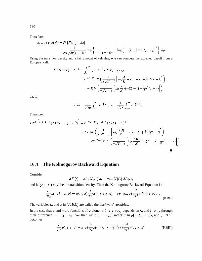
180
Therefore,O /214DXPQ1IJRGPSX3w,(S95 t u=v -C/A1I3xN,?S5 Ti S U VXW /21I6LY14D3 Z\(] ^ L TV /21I6LN14Dk3 i f A. SG L/cjL If(i f 3/A1 I Lg1 D 3Q f h ,(SBUsing the transitiondensityand a fair amountof calculus,onecan computethe expectedpayoff from aEuropeancall: t a /-0/|3[L0N3+C5 dD /`SLpN3+ O /21JPe9RGP4S.3,(S5w`+G Tiq dLN1 AX G ;=j(/&=L¡143q; If.i f /dLN143 E¢LMg Ti pLY1 £A. G ;j(/pLY143L If?i f /&=LY143 ¢where C/c¤?3[5 T VXW C¥
If E¦ ,(G%5 T V.W ¥ If E¦ ,(GB
Therefore,t D § $ w` /-C/&|3[L0N3+ '''' ¨ /2143 * 5 wcet ©£` /-0/|3wLCN3e5d-C/A143eª Ti dLN1 $ AX -C/A143 ;pj(/pLY143q; If i f /&dLg143 * ¢LM w` « Ti =LY1 $ AX -C/A143 ;dj(/&=LN143wL If(i f /pLg143 * ¢
16.4 The Kolmogorov Backward Equation
Consider ü¬ý ¬ ü¬ýjÿ üý ýw ü¬ýaÿ ü¬ý 6® ü¬ý ÿandlet
ûgü¬ýPþÿý J ÿ bethetransitiondensity. ThentheKolmogorov BackwardEquationis:¯±°° ýPþ ûgü¬ý;þÿEý ÿ ²¬ ü¬ý;þÿ °° ûgüýPþÿý ÿ ³ ³ ü¬ýPþÿ ° ³° ³ ûgü¬ý;þÿý | ÿ E (KBE)
Thevariablesý;þ
and inü´ ® arecalledthebackward variables.
In thecasethat ¬ and arefunctionsof alone,ûgü¬ýPþÿý µ ÿ dependson
ý;þand
ýonly through
their difference¶ ý ¯ ý þ. We thenwrite
ûgü ¶ Y ÿ ratherthanûgüý þ ÿý Y ÿ , and
ü´ ® becomes °° ¶ ûgü ¶ ÿ ¬ ü °° ûgü ¶ ÿ ³ ³ ü ° ³° ³ ûgü ¶ ÿ E (KBE’)
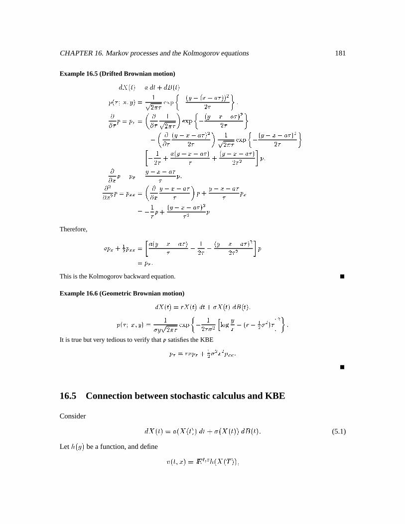
CHAPTER16. Markov processesandtheKolmogorov equations 181
Example16.5(Drifted Brownian motion),.-0/214365879,:1<;d,(>%/A143O /`·<R¸GP4S.365 T V.W · Z\(] ^ L /cSL/`G9;=7(·3e3+fV · h B¹¹ · O 5 Oº 5 ¹¹ · T V.W · ¢ Z\(] ^ L /cSLpG»LC7?·¼3efV · hL ¹¹ · /`SaLpG»L07(·3+fV · ¢ T VXW · Z\(] ^ L /`SLpG»LC7(·3efV · h5 $ L«TV · ; 7/`SFL0G»Lp7(·3· ; /`SLpG»LC7(·3V · f * O B¹¹ G O 5 O 5 SL0G½LM7(·· O B¹ f¹ G f O 5 O J 5 ¹¹ G SFL0G»Lp7(·· ¢ O ; SaLMG½L07(·· O 5¾L T· O ; /cSLCG»Lp7?·¼3ef· f O BTherefore, 7 O ; If O J 5 $ 7/cSL0G½LM7(·3· L TV · ; /`SaLMG½L07(·3efV · f * O5 O º BThis is theKolmogorov backwardequation.
Example16.6(GeometricBrownian motion),X-C/214365Kjk-C/2143l,:1m; i -C/A143,(>%/A143BO /c·qR6GP4S.365 Ti S VXW · Z\(] ^ L TV · i f AA. SG Lb/cjL If(i f 3+·( f h BIt is truebut very tediousto verify that
OsatisfiestheKBEOº 5KjEG O ; If i f G f O k B
16.5 Connectionbetweenstochasticcalculusand KBE
Consider ü¬ý ¬ ü üý ýw ü ü¬ý l® üý E (5.1)
Let ü bea function,anddefine ¿ ü¬ýjÿ ü ücÀ ÿ
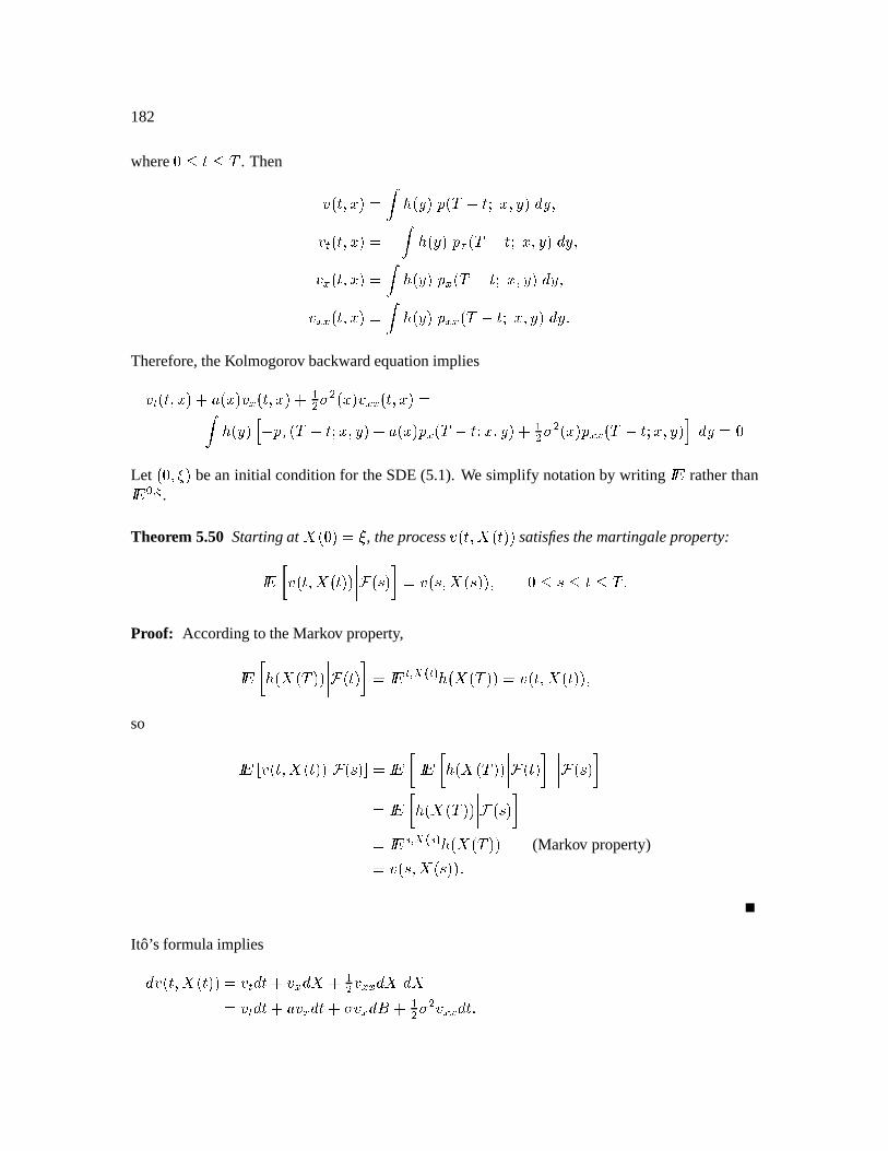
182
whereN ý À . Then ¿ ü¬ýjÿ ü ûgücÀ ¯ ý µ ÿ l ÿ¿ ü¬ýjÿ ¯ ü û ücÀ ¯ ý | ÿ ÿ¿ ü¬ýjÿ ü û ücÀ ¯ ý ÿ ÿ¿ E ü¬ýjÿ ü û E ücÀ ¯ ý ÿ Therefore,theKolmogorov backwardequationimplies¿ ü¬ýaÿ ¬ ü ¿ üýjÿ ³ ³ ü ¿ E ü¬ýaÿ ü ¯ û ücÀ ¯ ý k ÿ ¬ ü û ücÀ ¯ ý J ÿ ³ ³ ü û E ücÀ ¯ ý J ÿ Let
ü ÿ " beaninitial conditionfor theSDE(5.1). We simplify notationby writing
ratherthan þ #.
Theorem 5.50 Startingat ü l " , theprocess
¿ ü¬ýaÿ ü¬ý satisfiesthemartingaleproperty: $ ¿ ü¬ýjÿ üý ('''' ) üÁ * ¿ üÁ¢ÿ üÁ ÿ ! Á ý À Proof: Accordingto theMarkov property, $ ü ücÀ '''' ) ü¬ý * Â Ã»Ä ü ücÀ ¿ ü¬ýjÿ üý ÿso ÆÅ ¿ ü¬ýaÿ ü¬ý XÇ ) üÁ 4ȸ $ $ ü ücÀ '''' ) ü¬ý *'''' ) üÁ * $ ü ücÀ '''' ) üÁ * ¬ Ã»Ä ¬® ü üÉÀ (Markov property) ¿ üQÁÿ üÁ EIto’s formulaimplies ¿ üýjÿ ü¬ý w ¿ ýw ¿ ³ ¿ E ¿ ýw ¬ ¿ ý¸ ¿ ® ³ ³ ¿ E ý
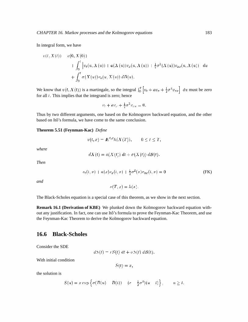
CHAPTER16. Markov processesandtheKolmogorov equations 183
In integral form, wehave¿ ü¬ýaÿ ü¬ý 6 ¿ ü ÿ ü þ ¿ üÊÿ üÊ ¬ ü üÊ ¿ üÊÿ üÊ ³ ³ ü üÊ ¿ E üÊÿ üQÊ Ê þ ü üÊ ¿ üÊ*ÿ üÊ 6® üÊ :We know that
¿ ü¬ýaÿ ü¬ý is a martingale,sotheintegral Ë þ ¿ ¬ ¿ ³ ³ ¿ E Ê mustbezerofor all
ý. This impliesthattheintegrandis zero;hence¿ ¬ ¿ ³ ³ ¿ E
Thusby two differentarguments,onebasedon theKolmogorov backwardequation,andtheotherbasedon Ito’s formula,we havecometo thesameconclusion.
Theorem 5.51(Feynman-Kac) Define¿ üýjÿ l  ? ü ücÀ ÿ ! ý Àöÿwhere ü¬ý ¬ ü üý ýw ü ü¬ý l® üý EThen ¿ ü¬ýaÿ ¬ ü ¿ ü¬ýjÿ ³ ³ ü ¿ E üýjÿ (FK)
and¿ üÉÀöÿ 6 ü E
TheBlack-Scholesequationis aspecialcaseof this theorem,aswe show in thenext section.
Remark 16.1(Derivation of KBE) We plunkeddown the Kolmogorov backwardequationwith-outany justification.In fact,onecanuseIto’sformulato prove theFeynman-KacTheorem,andusetheFeynman-KacTheoremto derive theKolmogorov backwardequation.
16.6 Black-Scholes
ConsidertheSDE Ì ü¬ý Í(Ì üý ý¸ Ì ü¬ý ® ü¬ý EWith initial condition Ì ü¬ý ÿthesolutionis Ì üÊ FÎEÏmÐ%Ñ ü ® üÊ ¯ ® ü¬ý xü Í ¯ ³ ³ üÊ ¯ ý EÒ ÿ ÊCÓý
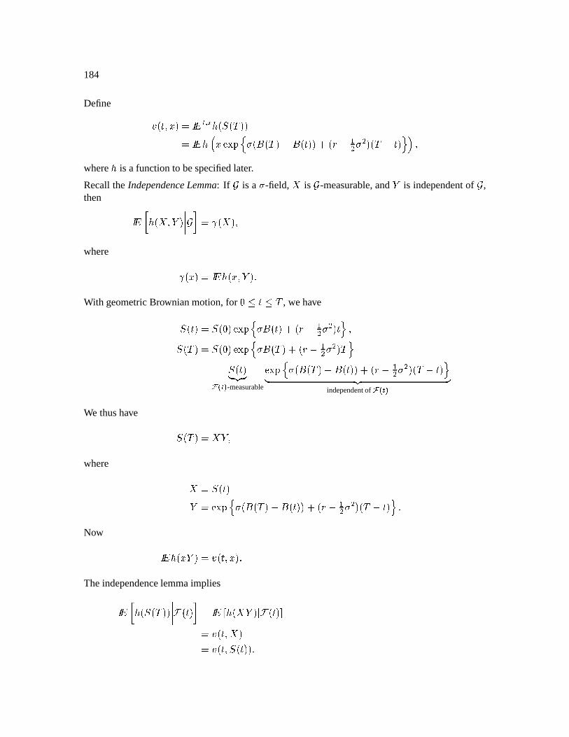
184
Define ¿ ü¬ýaÿ l Q ? ü Ì ücÀ ÔMÕ FÎEÏmÐ Ñ ü ® ücÀ ¯ ® ü¬ý xü Í ¯ ³ ³ ücÀ ¯ ý ÒqÖ ÿwhere
is a functionto bespecifiedlater.
Recallthe IndependenceLemma: If × is a -field, is × -measurable,and Ø is independentof × ,then $ ü ÿ Ø '''' × * ÚÙ ü ÿwhere Ù ü ! ü ÿ Ø EWith geometricBrownianmotion,for ! ý À , wehaveÌ üý Ì ü qÎEÏqÐ9Ñ ® ü¬ý xü Í ¯ ³ ³ ý Ò ÿ
Ì ücÀ Ì ü qÎEÏqÐ9Ñ ® ücÀ ü Í ¯ ³ ³ À Ò Ì ü¬ý Û ÜkÝ Þß ÄA -measurable
ÎEÏqÐ Ñ ü ® ücÀ ¯ ® ü¬ý ü Í ¯ ³ ³ ücÀ ¯ ý ÒÛ ÜJÝ Þindependentof
ß ÄA We thushave Ì ücÀ dØ ÿwhere Ì ü¬ý Ø ÚÎEÏqÐ Ñ ü ® ücÀ ¯ ® ü¬ý xü Í ¯ ³ ³ ücÀ ¯ ý Ò Now ! ü Ø ¿ ü¬ýjÿ ETheindependencelemmaimplies $ ü Ì ücÀ '''' ) ü¬ý * àÅ£ ü dØ XÇ ) ü¬ý QÈ ¿ ü¬ýjÿ ¿ ü¬ýjÿ Ì ü¬ý E
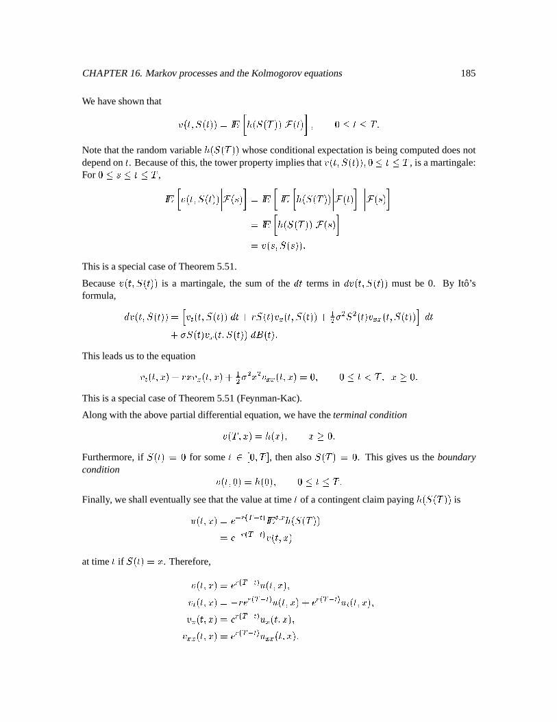
CHAPTER16. Markov processesandtheKolmogorov equations 185
We haveshown that ¿ ü¬ýjÿ Ì ü¬ý l á$c ü Ì ücÀ ('''' ) ü¬ý +* ÿ g ý À Notethattherandomvariable
ü Ì ücÀ whoseconditionalexpectationis beingcomputeddoesnotdependon
ý. Becauseof this, thetowerpropertyimpliesthat
¿ üýjÿ Ì ü¬ý ÿ % ý À , is amartingale:For ! Á ý À , $ ¿ ü¬ýaÿ Ì üý '''' ) üÁ * $ $ ü Ì ücÀ '''' ) ü¬ý * '''' ) üQÁ * â$c ü Ì ücÀ ('''' ) üÁ +* ¿ üÁÿ Ì üÁ EThis is aspecialcaseof Theorem5.51.
Because
¿ ü¬ýaÿ Ì ü¬ý is a martingale,the sum of the ý termsin ¿ ü¬ýaÿ Ì üý must be 0. By Ito’sformula, ¿ üýjÿ Ì ü¬ý 6 ¿ ü¬ýjÿ Ì ü¬ý ýw Í?Ì ü¬ý ¿ ü¬ýjÿ Ì ü¬ý ³ ³ Ì ³ ü¬ý ¿ E ü¬ýaÿ Ì ü¬ý ý Ì ü¬ý ¿ ü¬ýjÿ Ì ü¬ý l® üý EThis leadsusto theequation¿ ü¬ýjÿ Í( ¿ ü¬ýjÿ ³ ³ ³ ¿ E ü¬ýaÿ ÿ N ý9ãÀ+ÿ Ó This is aspecialcaseof Theorem5.51(Feynman-Kac).
Along with theabove partialdifferentialequation,wehave theterminalcondition¿ üÉÀöÿ 6 ü ÿ Ó Furthermore,if Ì ü¬ý for some
ý¡ä Å ÿÀ È , thenalso Ì ücÀ Â . This givesus the boundarycondition
¿ ü¬ýaÿ ü ÿ ! ý À Finally, weshalleventuallyseethatthevalueat time
ýof a contingentclaimpaying
ü Ì ücÀ isÊnü¬ýjÿ å(æqç ÄAè æ Q ? ü Ì ücÀ å(æqç ÄAè æ ¿ ü¬ýaÿ at time
ýif Ì ü¬ý . Therefore,¿ ü¬ýjÿ å ç ÄAè æ Ênü¬ýjÿ ÿ¿ ü¬ýjÿ ¯ Í(å ç ÄAè æ Êgüýjÿ å ç ÄAè æ Ê ü¬ýjÿ ÿ¿ ü¬ýjÿ åEç ÄAè æ Ê üýjÿ ÿ¿ E ü¬ýjÿ åEç ÄAè æ Ê E üýjÿ E
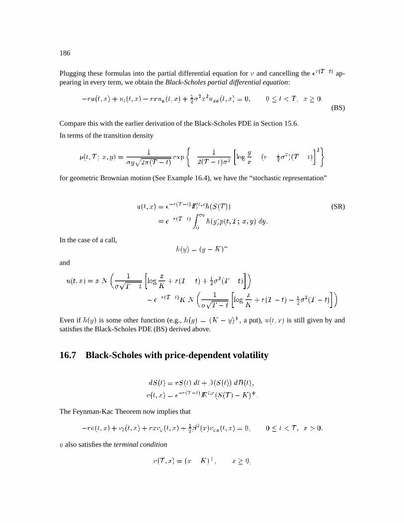
186
Pluggingtheseformulasinto the partialdifferentialequationfor
¿andcancellingthe å ç Äè æ ap-
pearingin every term,weobtaintheBlack-Scholespartial differentialequation:¯ Í Êgü¬ýaÿ Ê ü¬ýaÿ Í( Ê ü¬ýjÿ ³ ³ ³ Ê E ü¬ýjÿ ÿ g ýãÀöÿ Ó (BS)
Comparethiswith theearlierderivationof theBlack-ScholesPDEin Section15.6.
In termsof thetransitiondensityûnü¬ýjÿÀ ÿ é U êë üÉÀ ¯ ý ÎEÏqÐì ¯ éê ücÀ ¯ ý ³ $íî¼ï ¯ ü Í ¯ ³ ³ ücÀ ¯ ý * ³ðfor geometricBrownianmotion(SeeExample16.4),wehave the“stochasticrepresentation”Ênü¬ýjÿ Úå æqç ÄAè æ Q ü Ì ücÀ (SR)Úå(æqç ÄAè æ pñþ ü ûnü¬ýjÿÀ l ÿ In thecaseof acall, ü ü ¯ ´ òandÊgü¬ýaÿ lYó é6ô À ¯ ý $íî¼ï ´ Í ücÀ ¯ ý ³ ³ ücÀ ¯ ý * ¢
¯ å(æqç ÄAè æ ´ ó é ô À ¯ ý $íAîï ´ Í ücÀ ¯ ý ¯ ³ ³ üÉÀ ¯ ý * ¢Even if
ü is someotherfunction (e.g., ü % ü´ ¯ ò , a put),
Êgüýjÿ is still givenby andsatisfiestheBlack-ScholesPDE(BS) derivedabove.
16.7 Black-Scholeswith price-dependentvolatility
Ì ü¬ý l²Í?Ì ü¬ý ý¸¾õü Ì ü¬ý ® ü¬ý ÿ¿ üýjÿ l²å æqç Äè æ ü Ì ücÀ ¯ ´ ò TheFeynman-KacTheoremnow impliesthat¯ Í ¿ üýjÿ ¿ üýjÿ Í? ¿ üýjÿ ³ õ ³ ü ¿ E ü¬ýaÿ ÿ N ýãÀ+ÿ Cö ¿
alsosatisfiestheterminalcondition¿ ücÀ+ÿ [ ü ¯ ´ ò ÿ Ó ÿ
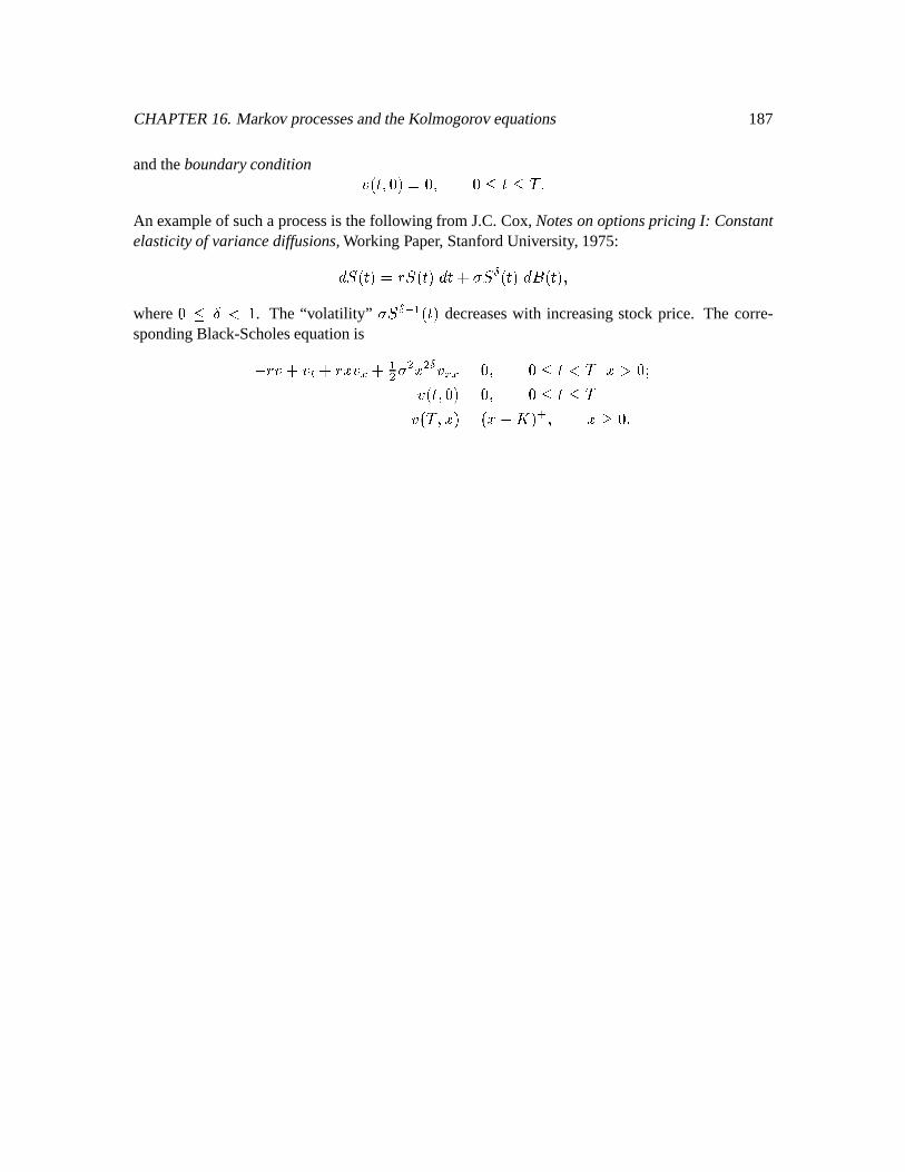
CHAPTER16. Markov processesandtheKolmogorov equations 187
andtheboundarycondition¿ üýjÿ l ÿ ! ý À
An exampleof sucha processis thefollowing from J.C.Cox,Notesonoptionspricing I: Constantelasticityof variancediffusions,Working Paper, StanfordUniversity, 1975:Ì ü¬ý ²Í?Ì ü¬ý ý¸ Ì|÷ ü¬ý |® ü¬ý ÿwhere ¾ ùø ã é . The “volatility” Ì ÷ æ ü¬ý decreaseswith increasingstockprice. The corre-spondingBlack-Scholesequationis¯ Í ¿ ¿ Í? ¿ ³ ³ ³ ÷ ¿ E ÿ ! ýãÀ =ö ¿ ü¬ýaÿ ÿ ! ý À¿ üÉÀöÿ 6 ü ¯ ´ ò ÿ Ó

188
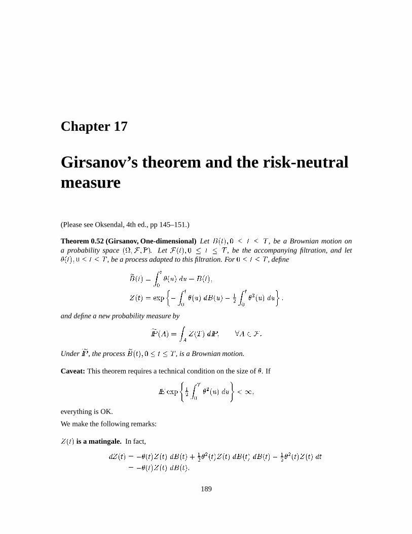
Chapter 17
Girsanov’s theoremand the risk-neutralmeasure
(PleaseseeOksendal,4th ed.,pp145–151.)
Theorem 0.52(Girsanov, One-dimensional) Let ® ü¬ý ÿ ² ý À, be a Brownian motion on
a probability spaceüQúöÿ ) ÿû . Let ) ü¬ý ÿ ü ý À
, be the accompanyingfiltration, and letý ü¬ý ÿ ! ý À , bea processadaptedto thisfiltration. For N ý À , defineþ® ü¬ý þ ý üÊ Ê ® ü¬ý ÿÿ ü¬ý ÚÎEÏmÐ ^ ¯ þ ý üÊ ® üÊ ¯ ³ þ ý ³ üÊ Ê h ÿanddefinea new probabilitymeasureby ü ÿ ücÀ ÿ Hä ) Under
, theprocess
þ® üý ÿ ý À , is a Brownianmotion.
Caveat: This theoremrequiresa technicalconditionon thesizeofý. If ÎEÏqÐì ³ èþ ý ³ üÊ Ê ð ãrÿ
everythingis OK.
We makethefollowing remarks:ÿ ü¬ý is a matingale. In fact, ÿ ü¬ý | ¯ ý ü¬ý ÿ ü¬ý ® ü¬ý ³ ý ³ ü¬ý ÿ ü¬ý ® ü¬ý ® ü¬ý ¯ ³ ý ³ ü¬ý ÿ üý ý ¯ ý ü¬ý ÿ ü¬ý ® ü¬ý E189
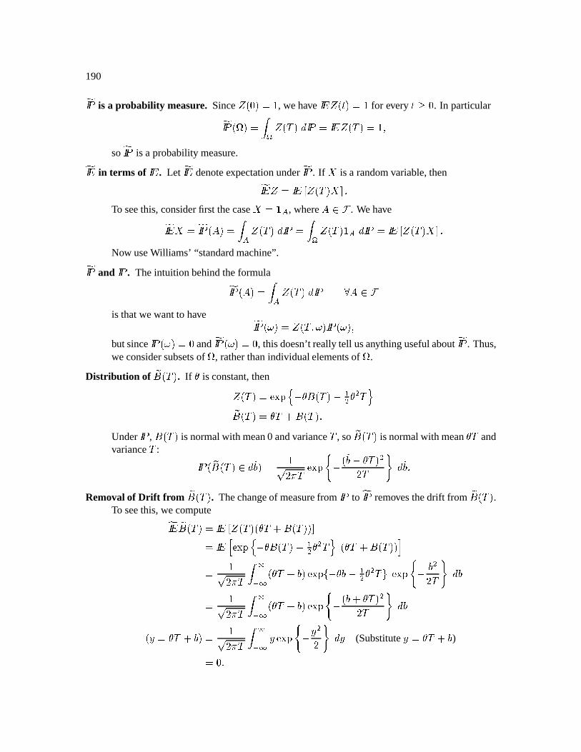
190 is a probability measure. Since
ÿ ü é , wehave !ÿ üý é for every
ýµÓ . In particular üú ÿ ücÀ !ÿ üÉÀ é ÿso
is a probabilitymeasure. in terms of
. Let
denoteexpectationunder
. If is a randomvariable,then Ôÿ ÆÅ£ÿ ücÀ È
To seethis,considerfirst thecase , where ä ) . Wehave ü ÿ ücÀ ² ÿ ücÀ ÆÅÿ ücÀ È
Now useWilliams’ “standardmachine”. and
. Theintuition behindtheformula ü ÿ ücÀ Hä )
is thatwewantto have ü | ÿ ücÀ+ÿ ü ÿbut since
ü and ü | , thisdoesn’t reallytell usanythingusefulabout
. Thus,
weconsidersubsetsofú
, ratherthanindividualelementsofú
.
Distrib ution ofþ® ücÀ . If
ýis constant,thenÿ ücÀ ÎEÏmÐ Ñ ¯ ý ® ücÀ ¯ ³ ý ³ À Òþ® ücÀ ý À ® üÉÀ E
Under
, ® ücÀ is normalwith mean0 andvarianceÀ
, soþ® üÉÀ is normalwith mean
ý Àand
varianceÀ
: ü þ® ücÀ ä éô êë À ÎEÏmÐ ì ¯ ü ¯ ý À ³ê À ð Removalof Drift fr om
þ® ücÀ . Thechangeof measurefrom
to
removesthedrift fromþ® ücÀ .
To seethis,wecompute þ® ücÀ àÅ£ÿ ücÀ ü ý À ® ücÀ +È ÎEÏqÐ Ñ ¯ ý ® ücÀ ¯ ³ ý ³ À Ò ü ý À ® ücÀ éô ê¼ë À ñæ ñ ü ý À <ÎEÏmÐ ¯ ý ¯ ³ ý ³ À ÎEÏmÐì ¯ ³ê À ð éô ê¼ë À ñæ ñ ü ý À <ÎEÏmÐ%ì ¯ ü ý À ³ê À ð ü ý À éô ê¼ë À dñæ ñ ÎEÏqÐì ¯
³ê ð (Substitute ý À )
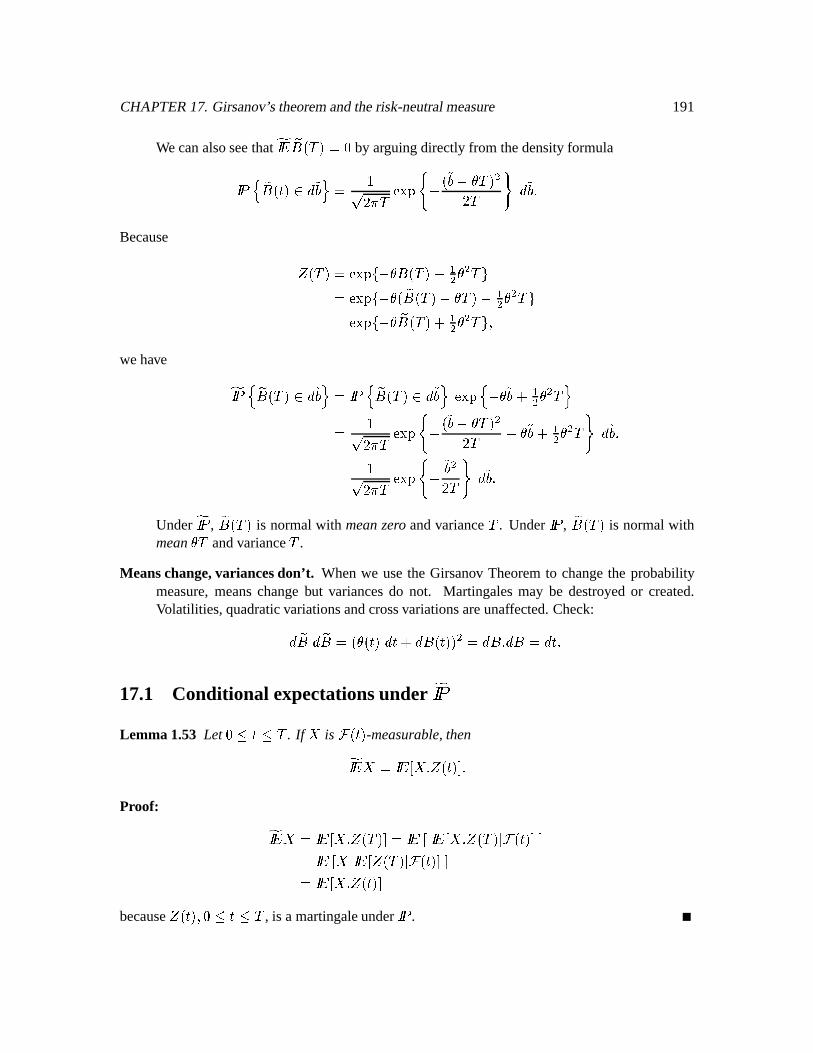
CHAPTER17. Girsanov’s theoremandtherisk-neutralmeasure 191
Wecanalsoseethat þ® ücÀ by arguingdirectly from thedensityformula Ñ þ® üý ä ÒY éô êë À ÎEÏqÐì ¯ ü ¯ ý À ³ê À ð
Because ÿ üÉÀ ÚÎEÏqÐ ¯ ý ® ücÀ ¯ ³ ý ³ ÀÚÎEÏqÐ ¯ ý ü þ® ücÀ ¯ ý À ¯ ³ ý ³ ÀÚÎEÏqÐ ¯ ý þ® ücÀ ³ ý ³ À/ÿwehave Ñ þ® ücÀ ä ÒY Ñ þ® üÉÀ ä Ò8ÎEÏqÐ%Ñ ¯ ý ³ ý ³ À Ò éô êë À ÎEÏqÐì ¯ ü ¯ ý À ³ê À ¯ ý ³ ý ³ À ð
éô êë À ÎEÏqÐì ¯ ³ê À ð Under
,þ® üÉÀ is normalwith meanzero andvariance
À. Under
,þ® ücÀ is normalwith
meaný À
andvarianceÀ
.
Meanschange,variancesdon’t. Whenwe usethe Girsanov Theoremto changethe probabilitymeasure,meanschangebut variancesdo not. Martingalesmay be destroyedor created.Volatilities,quadraticvariationsandcrossvariationsareunaffected.Check: þ® þ® ü ý ü¬ý | ý¸ ® üý ³ ®N® ý
17.1 Conditional expectationsunder
Lemma 1.53 Let ! ý À . If is ) üý -measurable,then YÅ ÿ ü¬ý 4È4Proof: YÅ ÿ ücÀ +È àÅ YÅ ÿ ücÀ XÇ ) üý +ÈqÈ àÅ YÅ£ÿ ücÀ XÇ ) üý +ÈqÈ YÅ ÿ ü¬ý 4Èbecause
ÿ ü¬ý ÿ ! ý À , is a martingaleunder
.
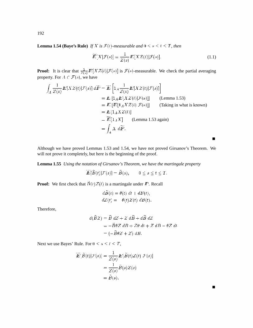
192
Lemma 1.54(Baye’sRule) If is ) ü¬ý -measurableand ! Á ý À , then YÅ Ç ) üQÁ +ȸ éÿ üÁ ¡Å ÿ ü¬ý XÇ ) üQÁ +È4 (1.1)
Proof: It is clearthat
Ä ¬® YÅ ÿ üý XÇ ) üQÁ +È is ) üÁ -measurable.We checkthe partialaveragingproperty. For
ä ) üÁ , wehave éÿ üÁ YÅ ÿ üý XÇ ) üQÁ +ȸ $ éÿ üÁ ¡Å ÿ ü¬ý XÇ ) üÁ +È * ÚÅ ¡Å ÿ ü¬ý XÇ ) üÁ +È&È (Lemma1.53) ÚÅ ¡Å ÿ ü¬ý XÇ ) üÁ +È&È (Takingin whatis known) ¡Å ÿ ü¬ý +È ¡Å È (Lemma1.53again) Although we have proved Lemmas1.53and1.54,we have not proved Girsanov’s Theorem.Wewill not prove it completely, but hereis thebeginningof theproof.
Lemma 1.55 Usingthenotationof Girsanov’sTheorem,wehavethemartingaleproperty YÅ þ® üý XÇ ) üÁ +ȸ þ® üÁ ÿ N Á ý À Proof: We first checkthat
þ® ü¬ý ÿ üý is amartingaleunder
. Recall þ® ü¬ý ý üý | ý¸ ® ü¬ý ÿ ÿ ü¬ý ¯ ý ü¬ý ÿ ü¬ý µ® üý ETherefore, ü þ® ÿ þ®« ÿ ÿ þ® þ®H ÿ ¯ þ® ý ÿ ® ÿ ý ýw ÿ ® ¯ ý ÿ ý ü ¯ þ® ý ÿ ÿ ®gNext weuseBayes’Rule.For ! Á ý À , gÅ þ® ü¬ý XÇ ) üÁ +ȸ éÿ üÁ ¡Å þ® ü¬ý ÿ üý XÇ ) üÁ QÈ éÿ üÁ þ® üÁ ÿ üÁ þ® üÁ :
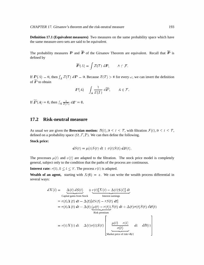
CHAPTER17. Girsanov’s theoremandtherisk-neutralmeasure 193
Definition 17.1(Equivalent measures) Two measureson thesameprobabilityspacewhich havethesamemeasure-zerosetsaresaidto beequivalent.
The probability measures
and
of the Girsanov Theoremareequivalent. Recall that
isdefinedby ü ÿ üÉÀ | ÿ ä ) If ü 9 , then Ë ÿ üÉÀ Because
ÿ ücÀ Fö for every
, we caninvert thedefinitionof
to obtain ü | éÿ ücÀ ÿ ä ) If ü , then Ë Äè
17.2 Risk-neutral measure
As usualwe aregiventheBrownian motion: ® ü¬ý ÿ = ý À, with filtration ) ü¬ý ÿ M ý À
,definedona probabilityspace
üú+ÿ ) ÿû . We canthendefinethefollowing.
Stockprice: Ì ü¬ý üý Ì ü¬ý ý¸"! üý Ì ü¬ý ® ü¬ý EThe processes üý and
!5üý are adaptedto the filtration. The stock price model is completelygeneral,subjectonly to theconditionthatthepathsof theprocessarecontinuous.
Interestrate: Í üý ÿ ! ý À . TheprocessÍ ü¬ý is adapted.
Wealth of an agent, startingwith ü N . We can write the wealthprocessdifferential inseveralways: ü¬ý # ü¬ý Ì ü¬ý Û ÜkÝ Þ
Capitalgainsfrom Stock
Í ü¬ý Å ü¬ý ¯ # ü¬ý Ì üý +È ýÛ ÜkÝ ÞInterestearnings²Í üý ü¬ý l ý¸ # ü¬ý Å Ì ü¬ý ¯ Í(Ì ü¬ý ý È²Í üý ü¬ý l ý¸ # ü¬ý ü ü¬ý ¯ Í ü¬ý Û ÜkÝ Þ
Riskpremium
Ì ü¬ý ýw # ü¬ý !5ü¬ý Ì ü¬ý l® üý ²Í üý ü¬ý l ý¸ # ü¬ý ! üý Ì ü¬ý $%%%%& ü¬ý ¯ Í ü¬ý !Kü¬ý Û ÜJÝ Þ
Marketpriceof risk= ÄA ý¸ ® ü¬ý '(((()
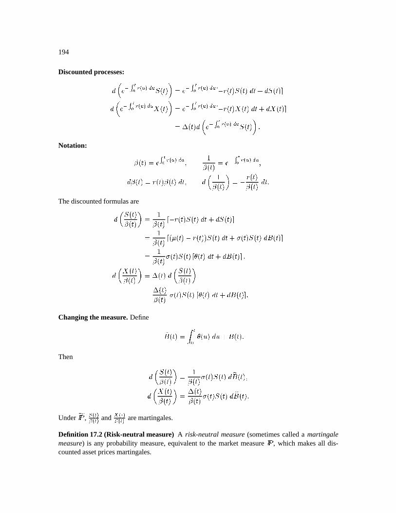
194
Discountedprocesses: å æ Ë+* ç Ä-, /. , Ì ü¬ý ¢ å æ Ë0* ç Ä-, . , Å ¯ Í ü¬ý Ì ü¬ý ý¸ Ì üý +È å æ Ë1* ç Ä-, 2. , ü¬ý ¢ å æ Ë0* ç Ä-, . , Å ¯ Í ü¬ý ü¬ý l ý¸ ü¬ý +È3# ü¬ý å æ Ë1* ç Ä4, . , Ì ü¬ý ¢ Notation: õüý |²å Ë1* ç Ä4, . , ÿ éõü¬ý ²å æ Ë* ç Ä-, /. , ÿ õü¬ý Í ü¬ý õIü¬ý ýjÿ éõIü¬ý ¢ ¯ Í ü¬ý õü¬ý ý Thediscountedformulasare Ì ü¬ý õü¬ý ¢ éõüý Å ¯ Í ü¬ý Ì ü¬ý l ý6 Ì ü¬ý 4È éõüý Å ü ü¬ý ¯ Í ü¬ý Ì ü¬ý l ý¸"!Kü¬ý Ì ü¬ý ® üý +È éõüý !5ü¬ý Ì ü¬ý Å ý üý | ý¸ ® ü¬ý 4È ÿ ü¬ý õü¬ý ¢ 3# üý Ì ü¬ý õüý ¢ # üý õüý !Kü¬ý Ì ü¬ý Å ý ü¬ý ýw ® ü¬ý +ÈChanging the measure. Define þ® üý |² þ ý üÊ Ê ® ü¬ý EThen Ì üý õIü¬ý ¢ éõü¬ý !5üý Ì ü¬ý þ® ü¬ý ÿ üý õIü¬ý ¢ # ü¬ý õü¬ý !5üý Ì ü¬ý þ® ü¬ý EUnder
, 5 ÄA 6 ÄA and
ûÄA 6 ÄA aremartingales.
Definition 17.2(Risk-neutral measure) A risk-neutral measure (sometimescalleda martingalemeasure) is any probability measure,equivalentto the marketmeasure
, which makesall dis-
countedassetpricesmartingales.
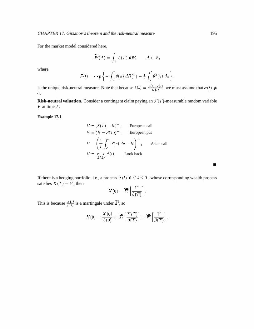
CHAPTER17. Girsanov’s theoremandtherisk-neutralmeasure 195
For themarketmodelconsideredhere, ü ÿ üÉÀ | ÿ ä ) ÿwhere ÿ ü¬ý |ÚÎEÏqÐ ^ ¯ þ ý üÊ ® üÊ ¯ ³ þ ý ³ üQÊ Ê h ÿis theuniquerisk-neutralmeasure.Notethatbecause
ý ü¬ý 87 ÄA æmç ÄA ! ÄA ÿwemustassumethat
!Kü¬ý 9 .Risk-neutral valuation. Consideracontingentclaimpayingan ) ücÀ -measurablerandomvariable:
at timeÀ
.
Example17.1 ; 5¾/=</&|3[L0g3ePEuropeancall
; 5¾/` L><l/|3e3+|PEuropeanput; 5@?!T D <l/BA3[,CA½L0ED P Asiancall; 5GFEH \DJI I </2143P Look back
If thereis ahedgingportfolio, i.e.,aprocess# ü¬ý ÿ  ý À , whosecorrespondingwealthprocesssatisfies ücÀ : , then ü l á$ :õüÉÀ *_This is because
Ã_ÄA 6 ÄA is amartingaleunder
, so
ü l ü õü $ ücÀ õücÀ * $ :õIücÀ *

196
Chapter 18
Martingale RepresentationTheorem
18.1 Martingale RepresentationTheorem
SeeOksendal,4th ed.,Theorem4.11,p.50.
Theorem 1.56 Let ® ü¬ý ÿ ! ý À+ÿbea Brownianmotionon
üúÿ ) ÿû . Let ) üý ÿ ! ý À , bethefiltrationgeneratedby thisBrownianmotion. Let ü¬ý ÿ ! ý À , bea martingale(under
)
relativeto thisfiltration. Thenthere is anadaptedprocessø ü¬ý ÿ  ý À , such that ü¬ý l ü þ ø üÊ ® üQÊ ÿ ! ý À In particular, thepathsof are continuous.
Remark 18.1 Wealreadyknow thatif üý is aprocesssatisfying ü¬ý ø ü¬ý ® ü¬ý ÿthen ü¬ý is amartingale.Now weseethatif ü¬ý is amartingaleadaptedto thefiltrationgeneratedby theBrownianmotion ® ü¬ý , i.e, theBrownianmotionis theonly sourceof randomnessin , then ü¬ý l ø üý |® üý for someø ü¬ý .18.2 A hedgingapplication
Homework Problem 4.5. In thecontext of Girsanov’sTheorem,suppsethat ) ü¬ý ÿ Y ý Àöÿis
thefiltration generatedby theBrownianmotion ® (under
). Supposethat Ø is a
-martingale.Thenthereis anadaptedprocessÙ ü¬ý ÿ  ý À , suchthatØ ü¬ý Ø ü þ Ù üÊ l þ® üÊ ÿ g ý À
197
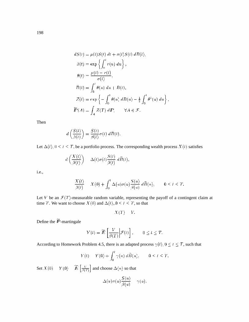
198
Ì ü¬ý l üý Ì ü¬ý ý¸"! üý Ì ü¬ý ® ü¬ý ÿõü¬ý ÎEÏmÐ ^ þ Í üÊ Ê h ÿý üý | üý ¯ Í üý ! üý ÿþ® ü¬ý þ ý üÊ | Ê% ® üý ÿÿ üý | ÎEÏmÐ ^ ¯ þ ý üQÊ |® üQÊ ¯ ³ þ ý ³ üÊ Ê h ÿ ü ÿ ücÀ ÿ ä )
Then Ì ü¬ý õü¬ý ¢ Ì ü¬ý õü¬ý ! ü¬ý þ® ü¬ý ELet # ü¬ý ÿ  ý Àöÿ
beaportfolio process.Thecorrespondingwealthprocess ü¬ý satisfies ü¬ý õü¬ý ¢ K# ü¬ý ! üý Ì ü¬ý õü¬ý þ® ü¬ý ÿi.e., ü¬ý õüý ü þ # üQÊ !KüÊ Ì üÊ õüQÊ þ® üQÊ ÿ g ý À Let:
be an ) üÉÀ -measurablerandomvariable,representingthe payoff of a contingentclaim attime
À. Wewantto choose ü and # üý ÿ ý À , sothat üÉÀ l :
Definethe
-martingale Ø ü¬ý á$ :õücÀ '''' ) ü¬ý 4* ÿ ! ý À Accordingto Homework Problem4.5,thereis anadaptedprocessÙ ü¬ý ÿ % ý À , suchthatØ ü¬ý Ø ü þ Ù üÊ l þ® üÊ ÿ g ý À Set ü l Ø ü >L6 ÄAè andchoose# üÊ sothat# üÊ !güQÊ Ì üÊ õüÊ ÚÙ üÊ :
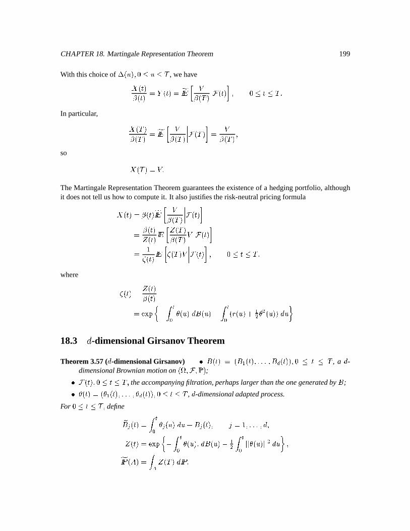
CHAPTER18. MartingaleRepresentationTheorem 199
With thischoiceof # üÊ ÿ Â Ê À , wehave ü¬ý õü¬ý Ø ü¬ý $ :õücÀ '''' ) ü¬ý * ÿ ! ý À In particular, ücÀ õücÀ $ :õIücÀ '''' ) ücÀ * :õücÀ ÿso ücÀ : TheMartingaleRepresentationTheoremguaranteestheexistenceof a hedgingportfolio, althoughit doesnot tell ushow to computeit. It alsojustifiestherisk-neutralpricing formula ü¬ý õü¬ý $ :õücÀ '''' ) üý * õüý ÿ ü¬ý $ ÿ ücÀ õüÉÀ : '''' ) ü¬ý * éM ü¬ý â$ M ücÀ : '''' ) ü¬ý +* ÿ N ý À+ÿwhere M ü¬ý ÿ ü¬ý õüý ÚÎEÏqÐ ^ ¯ þ ý üÊ ® üQÊ ¯ þ ü Í üÊ ³ ý ³ üQÊ Ê h18.3 N -dimensionalGirsanov Theorem
Theorem 3.57( -dimensionalGirsanov) O ® ü¬ý ü ® üý ÿ XX ÿ ® . üý ÿ Ú ý À, a -
dimensionalBrownianmotiononüúÿ ) ÿû ;O ) üý ÿ ý À+ÿ
theaccompanyingfiltration,perhapslarger thantheonegeneratedby ® ;O ý üý | ü ý ü¬ý ÿ X. ÿ ý . ü¬ý ÿ  ý À , -dimensionaladaptedprocess.
For ! ý Àöÿdefineþ®QP ü¬ý ² þ ý P üÊ Ê ®QP ü¬ý ÿ R é ÿ .X ÿ ÿÿ üý | ÎEÏmÐ ^ ¯ þ ý üQÊ E® üÊ ¯ ³ þ Ç&Ç ý üÊ XÇ&Ç ³ Ê h ÿ ü ÿ ücÀ
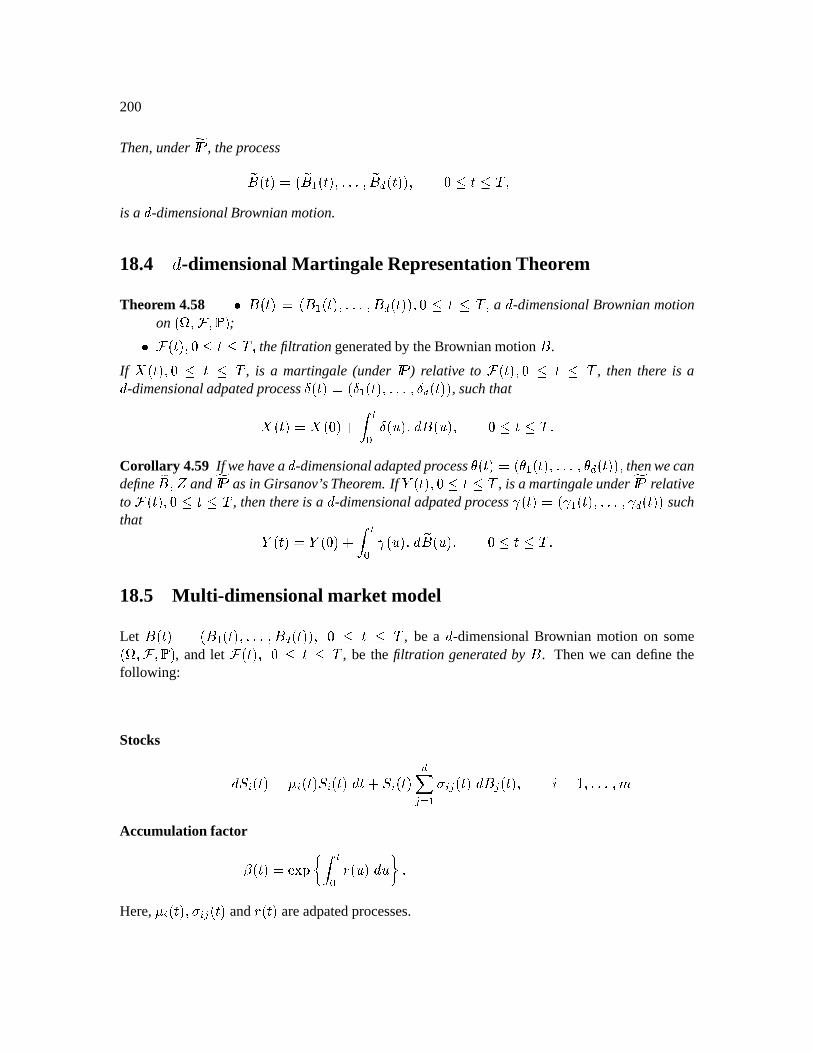
200
Then,under
, theprocessþ® ü¬ý ü þ® üý ÿ XX ÿ þ® . üý ÿ g ý Àöÿis a -dimensionalBrownianmotion.
18.4 N -dimensionalMartingale RepresentationTheorem
Theorem 4.58 O ® ü¬ý  ü ® ü¬ý ÿ .X ÿ ® . ü¬ý ÿ C ý Àöÿa -dimensionalBrownianmotion
onüúÿ ) ÿû ;O ) üý ÿ ý À+ÿ
thefiltrationgeneratedby theBrownianmotion ® .
If ü¬ý ÿ à ý À, is a martingale(under
) relative to ) ü¬ý ÿ Ú ý À
, then there is a -dimensionaladpatedprocessø ü¬ý | ü ø ·ü¬ý ÿ .X ÿ ø . üý , such that ü¬ý ü þ ø üQÊ E(® üÊ ÿ N ý À Corollary 4.59 If wehavea -dimensionaladaptedprocess
ý ü¬ý ü ý ü¬ý ÿ .X ÿ ý . ü¬ý ÿ thenwecandefine
þ® ÿ ÿand
asin Girsanov’sTheorem.If Ø ü¬ý ÿ ! ý À , is a martingaleunder
relativeto ) ü¬ý ÿ N ý À , thenthere is a -dimensionaladpatedprocessÙ ü¬ý ü Ù ·ü¬ý ÿ X. ÿ Ù . üý suchthat Ø üý Ø ü þ Ù üÊ E( þ® üÊ ÿ ! ý À 18.5 Multi-dimensional market model
Let ® ü¬ý ü ® ü¬ý ÿ X. ÿ ® . ü¬ý ÿ ý À, be a -dimensionalBrownian motion on someüúÿ ) ÿû , andlet ) üý ÿ ý À
, be the filtration generatedby ® . Thenwe candefinethefollowing:
Stocks Ì+S üý T+S ü¬ý Ì+S ü¬ý | ý¸ Ì+S ü¬ý .UPWV ! SXP üý |®YP ü¬ý ÿ Z é ÿ X. ÿ\[Accumulation factorõüý ÚÎEÏqÐ ^ þ Í üÊ Ê h Here, +S ü¬ý ÿ\! SXP ü¬ý and Í ü¬ý areadpatedprocesses.
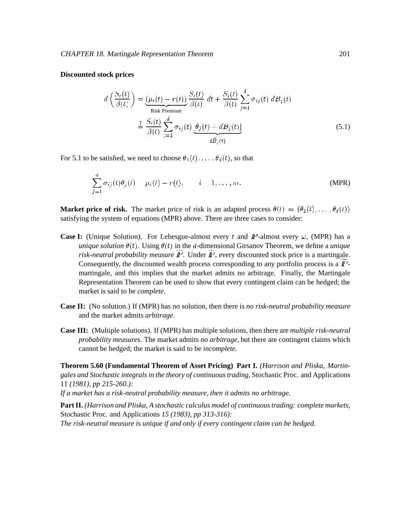
CHAPTER18. MartingaleRepresentationTheorem 201
Discountedstockprices
Ì S ü¬ý õü¬ý ¢ ü +S ü¬ý ¯ Í ü¬ý Û ÜJÝ ÞRisk Premium
Ì S ü¬ý õü¬ý ý¸ Ì S ü¬ý õü¬ý .UPWV ! SXP ü¬ý |®QP ü¬ý ] Ì+S ü¬ý õü¬ý .UPWV ! SXP üý Å ý P ü¬ý ®QP üý +ÈÛ ÜkÝ Þ. þ^_ ÄA (5.1)
For 5.1to besatisfied,weneedto chooseý ü¬ý ÿ X. ÿ ý . ü¬ý , sothat.UPJV ! SP ü¬ý ý P üý T+S ü¬ý ¯ Í ü¬ý ÿ Z é ÿ X. ÿ\[ (MPR)
Market price of risk. The marketprice of risk is an adaptedprocessý ü¬ý N ü ý ü¬ý ÿ X. ÿ ý . üý
satisfyingthesystemof equations(MPR)above. Therearethreecasesto consider:
CaseI: (Unique Solution). For Lebesgue-almosteveryý
and
-almostevery
, (MPR) hasauniquesolution
ý ü¬ý . Usingý ü¬ý in the -dimensionalGirsanov Theorem,wedefineaunique
risk-neutral probability measure
. Under
, every discountedstockprice is a martingale.Consequently, thediscountedwealthprocesscorrespondingto any portfolio processis a
-
martingale,and this implies that the marketadmitsno arbitrage. Finally, the MartingaleRepresentationTheoremcanbeusedto show thatevery contingentclaim canbehedged;themarketis saidto becomplete.
CaseII: (No solution.)If (MPR)hasnosolution,thenthereis no risk-neutral probabilitymeasureandthemarketadmitsarbitrage.
CaseIII: (Multiple solutions).If (MPR)hasmultiplesolutions,thentherearemultiplerisk-neutralprobabilitymeasures. Themarketadmitsnoarbitrage, but therearecontingentclaimswhichcannotbehedged;themarketis saidto be incomplete.
Theorem 5.60(FundamentalTheorem of AssetPricing) Part I. (Harrison and Pliska, Martin-galesandStochasticintegralsin thetheoryof continuoustrading,StochasticProc.andApplications11 (1981),pp215-260.):If a markethasa risk-neutral probabilitymeasure,thenit admitsnoarbitrage.
Part II. (HarrisonandPliska,Astochasticcalculusmodelofcontinuoustrading: completemarkets,StochasticProc.andApplications15(1983),pp313-316):Therisk-neutral measure is uniqueif andonly if everycontingentclaimcanbehedged.

202
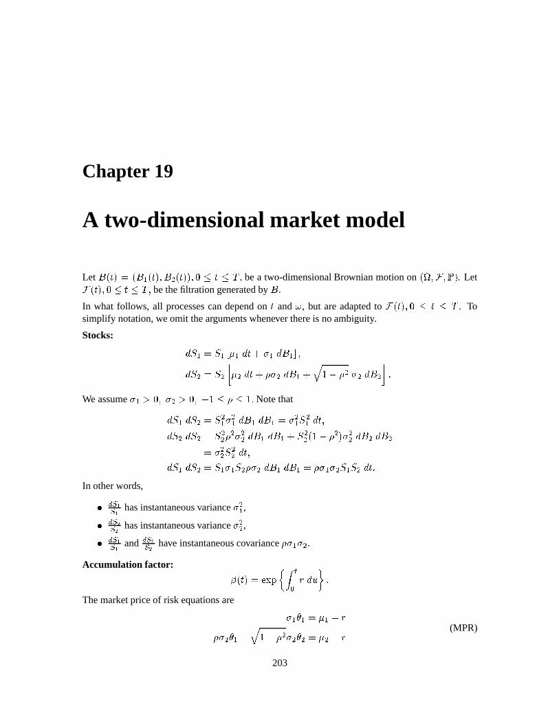
Chapter 19
A two-dimensionalmarket model
Let ® ü¬ý » ü ® ü¬ý ÿ ® ³ ü¬ý ÿ g ý Àöÿbea two-dimensionalBrownianmotionon
üú+ÿ ) ÿû . Let) ü¬ý ÿ ! ý Àöÿbethefiltration generatedby ® .
In what follows, all processescandependoný
and
, but areadaptedto ) ü¬ý ÿ ¾ ý À. To
simplify notation,weomit theargumentswhenever thereis noambiguity.
Stocks: Ì Ì Å ýw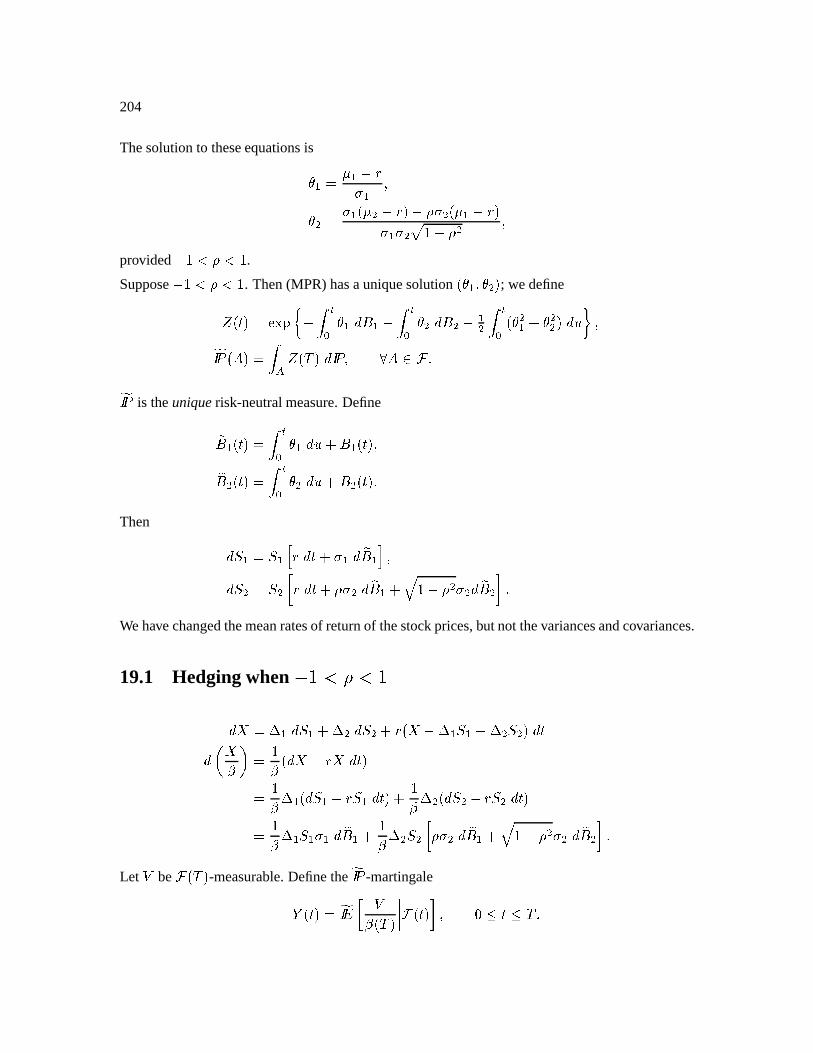
204
Thesolutionto theseequationsisý ¯ Í! ÿý ³ 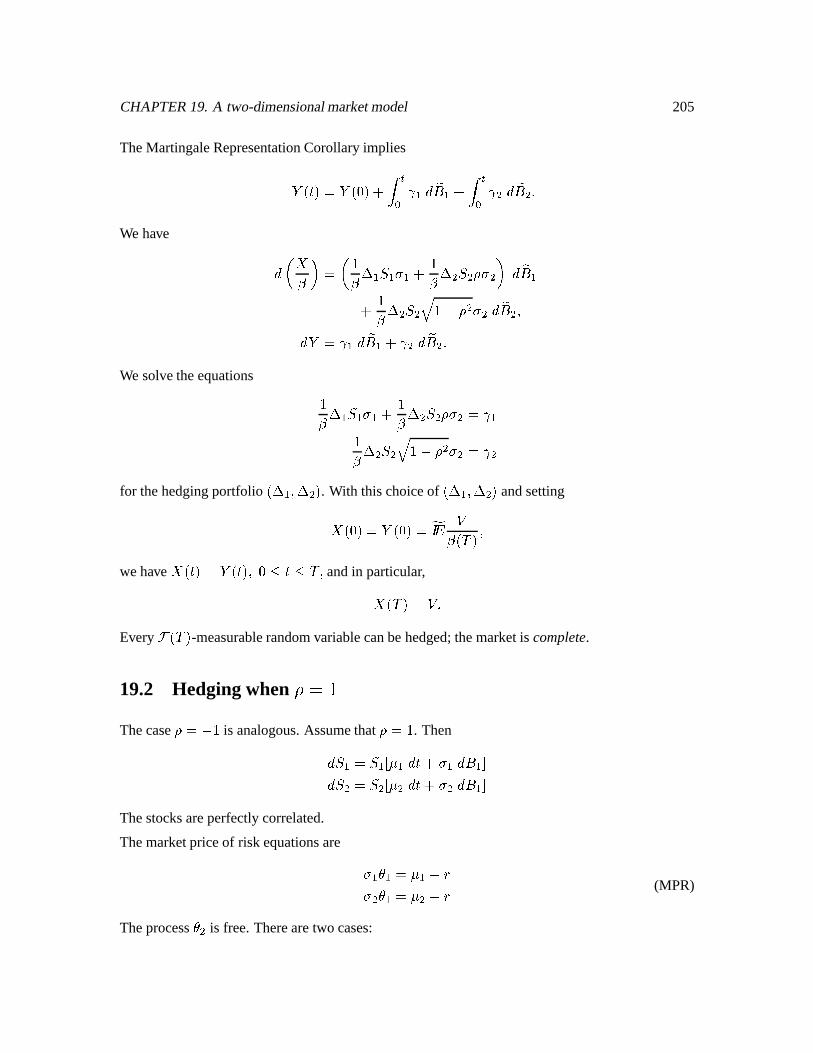
CHAPTER19. A two-dimensionalmarketmodel 205
TheMartingaleRepresentationCorollaryimplies
Ø üý | Ø ü þ Ù þ® l þ Ù ³ þ® ³ We have õ ¢ éõ # Ì J!l éõ # ³ Ì ³ `e! ³ ¢ þ® éõ # ³ Ì ³ c é ¯ ` ³ ! ³ þ® ³ ÿ Ø Ù þ® Ù ³ þ® ³ We solvetheequations éõ # Ì W! l éõ # ³ Ì ³ `b! ³ Ù éõ # ³ Ì ³ c é ¯ ` ³ ! ³ Ù ³for thehedgingportfolio
ü # ÿ # ³ . With thischoiceofü # ÿ # ³ andsetting ü l Ø ü :õücÀ ÿ
wehave ü¬ý Ø ü¬ý ÿ ! ý Àöÿandin particular, üÉÀ l :
Every ) üÉÀ -measurablerandomvariablecanbehedged;themarketis complete.
19.2 Hedgingwhen oKs mThecase ¯ é is analogous.Assumethat
` é . ThenÌ Ì Å ý¸"!6 ® ÈÌ ³ Ì ³ Å ³ ý¸"! ³ ® ÈThestocksareperfectlycorrelated.
Themarketpriceof risk equationsare ! ý T ¯ Í! ³ ý T ³ ¯ Í (MPR)
Theprocessý ³ is free.Therearetwo cases:
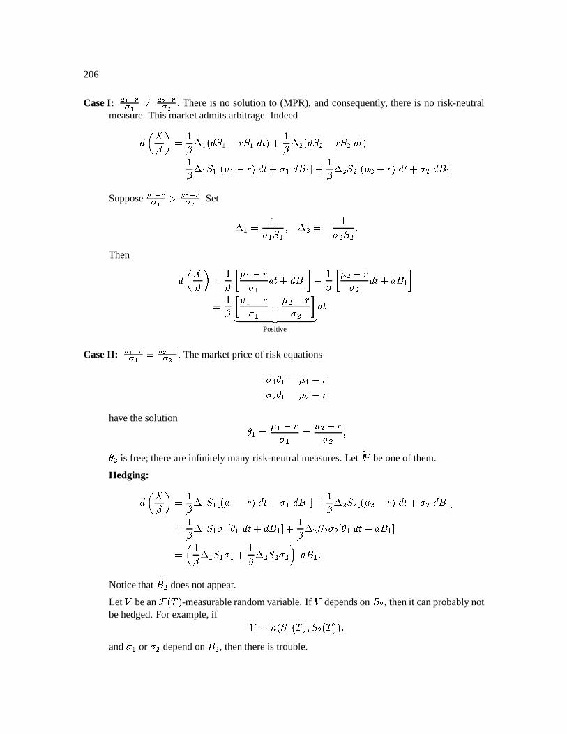
206
CaseI: 7 f æmç! f 9 7 g æqç! g Thereis no solutionto (MPR), andconsequently, thereis no risk-neutralmeasure.Thismarketadmitsarbitrage.Indeed õ ¢ éõ # ·ü Ì ¯ Í(Ì ý éõ # ³ ü Ì ³ ¯ Í(Ì ³ ý éõ # Ì Å ü ¯ Í( ý¸
CHAPTER19. A two-dimensionalmarketmodel 207
Moreprecisely, we definethe
-martingaleØ ü¬ý | â$ :õücÀ '''' ) ü¬ý +* ÿ g ý À We canwrite
Ø ü¬ý | Ø ü þ Ù þ® l þ Ù ³ þ® ³ ÿso Ø ÚÙ þ® l Ù ³ þ® ³ To get Õ Ã 6 Ö to match Ø , we musthaveÙ ³

208
Chapter 20
Pricing Exotic Options
20.1 Reflectionprinciple for Brownian motion
Without drift.
Define t ücÀ vuxw(Ïþhy y è ® ü¬ý EThenwehave: t ücÀ Fö [Lÿ ® ücÀ ã (® ücÀ »ö ê [ ¯ éô ê¼ë À ñ³z æ ÎEÏqÐì ¯ ³ê À ð ÿ [ ö ÿ ã[Sothejoint densityis
t ücÀ ä [Lÿ ® ücÀ ä ¯ ° ³° [ ° ? éô êë À ñ³Wz æ| ÎEÏmÐÂì ¯ ³ê À ð D [ ¯ °° [? éô êë À ÎEÏmÐ ì ¯ ü ê [ ¯ ³ê À ð D [ ÿ ê ü ê [ ¯ À ô êë À ÎEÏqÐì ¯ ü ê [ ¯ ³ê À ð [ ÿ [ ö ÿ ã[
With drift. Let þ® ü¬ý ý ýs ® ü¬ý ÿ209
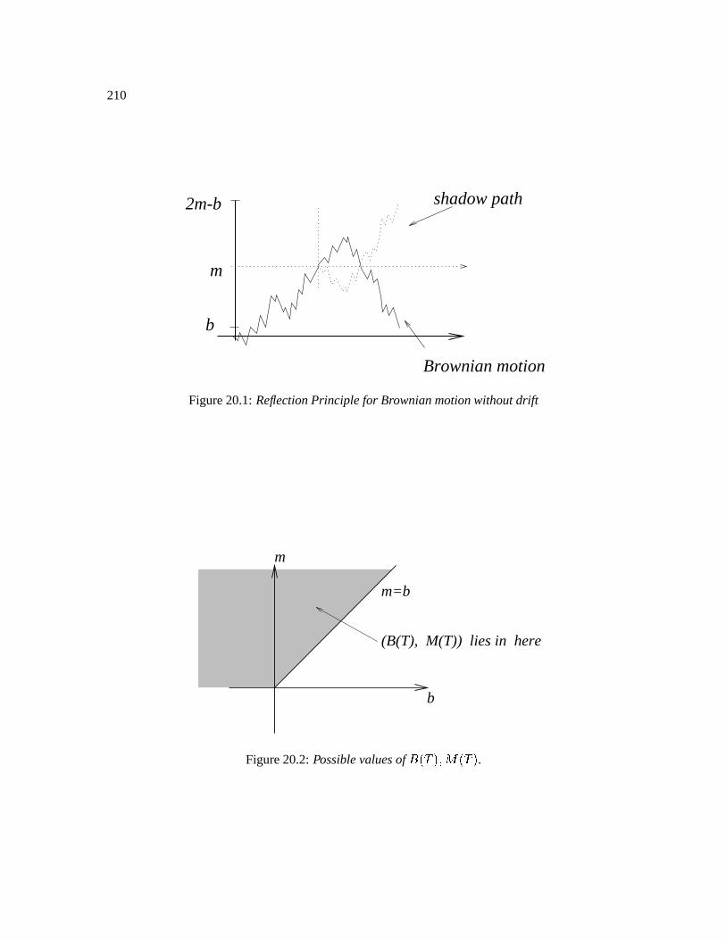
210
shadow path
m
Brownian motion
2m-b
b
Figure20.1:ReflectionPrinciple for Brownianmotionwithoutdrift
m=b
b
m
(B(T), M(T)) lies in here
Figure20.2:Possiblevaluesof ® ücÀ ÿ t ücÀ .
CHAPTER20. PricingExoticOptions 211
where® ü¬ý ÿ ! ý À , is a Brownianmotion(withoutdrift) onüú+ÿ ) ÿû . Defineÿ ücÀ ÚÎEÏqÐ+ ¯ ý ® ücÀ ¯ ³ ý ³ ÀÚÎEÏqÐ+ ¯ ý ü ® ücÀ ý À ³ ý ³ ÀÚÎEÏqÐ+ ¯ ý þ® ü¬ý ³ ý ³ À/ÿ ü ÿ üÉÀ ÿ ä )
Sett ücÀ 3u~w(Ï þiy y è þ® ücÀ E
Under ÿ þ® is aBrownianmotion(withoutdrift), so t üÉÀ ä [Âÿ þ® ücÀ ä ê ü ê [ ¯ À ô êë À ÎEÏqÐì ¯ ü ê [ ¯ ³ê À ð [ ÿ [ ö ÿ ã [
Let ü [Lÿ beafunctionof two variables.Then Ô ü t ücÀ ÿ þ® ücÀ ü t ücÀ ÿ þ® ücÀ ÿ ücÀ ü t ücÀ ÿ þ® ücÀ qÎEÏqÐe ý þ® ücÀ ¯ ³ ý ³ À
z V ñz V þ V z V æ ñ ü [Âÿ !ÎEÏqÐ ý ¯ ³ ý ³ À t ücÀ ä [Lÿ þ® ücÀ ä But also,
Ô ü t ücÀ ÿ þ® ücÀ z V ñz V þ V z V æ ñ ü [Âÿ t ücÀ ä [Âÿ þ® üÉÀ ä Since
is arbitrary, weconcludethat
(MPR)
t ücÀ ä [Lÿ þ® üÉÀ ä ÎEÏmÐ ý ¯ ³ ý ³ À t ücÀ ä [Çÿ þ® ücÀ ä ê ü ê [ ¯ À ô ê¼ë À ÎEÏqÐ ì ¯ ü ê [ ¯ ³ê À ð ÎEÏqÐ ý ¯ ³ ý ³ À [ / ÿ [ ö ÿ ã [
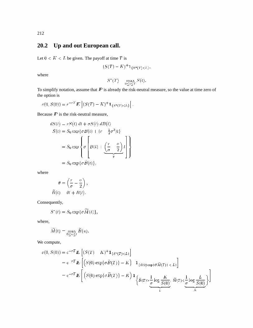
212
20.2 Up and out Europeancall.
Let ãÆ´ ãbegiven.Thepayoff at time
Àisü Ì ücÀ ¯ ´ òb 5 ÄAè be ÿ
where Ì ücÀ u~w(Ïþhy y è Ì ü¬ý :To simplify notation,assumethat
is alreadytherisk-neutralmeasure,sothevalueat timezeroof
theoptionis¿ ü ÿ Ì ü 6åæqç è ü Ì ücÀ ¯ ´ òd 5 ÄAè eb Because
is therisk-neutralmeasure,Ì ü¬ý Í(Ì ü¬ý ýw! Ì üý ® ü¬ý Ì ü¬ý Ì þ ÎEÏqÐ ! ® ü¬ý 'ü Í ¯ ³ ! ³ ýÌ þ ÎEÏqÐT
! $%%%& ® ü¬ý Í! ¯ ! ê ¢Û ÜkÝ Þý '((() Ì þ ÎEÏqÐ ! þ® ü¬ý /ÿ
where ý Í! ¯ ! ê ¢ ÿþ® ü¬ý | ý ý6 ® üý EConsequently,Ì ü¬ý |Ì þ ÎEÏqÐ ! t ü¬ý /ÿwhere, t ü¬ý |u~w(Ïþiy , y þ® üQÊ EWe compute,¿ ü ÿ Ì ü 6å æqç è ü Ì ücÀ ¯ ´ ò 5 ÄAè eb åæqç è á$ Õ Ì ü qÎEÏqÐe ! þ® ücÀ ¯ ´ Ö ò 5 Ä þ \ ! þ ÄAè B+e *å æqç è "6Õ Ì ü qÎEÏqÐ ! þ® ücÀ ¯ ´ Ö ^ þ^ Äè é! íî¼ï ´Ì ü Û ÜJÝ Þ þ Äè é! íAîï Ì ü Û ÜkÝ Þ h0
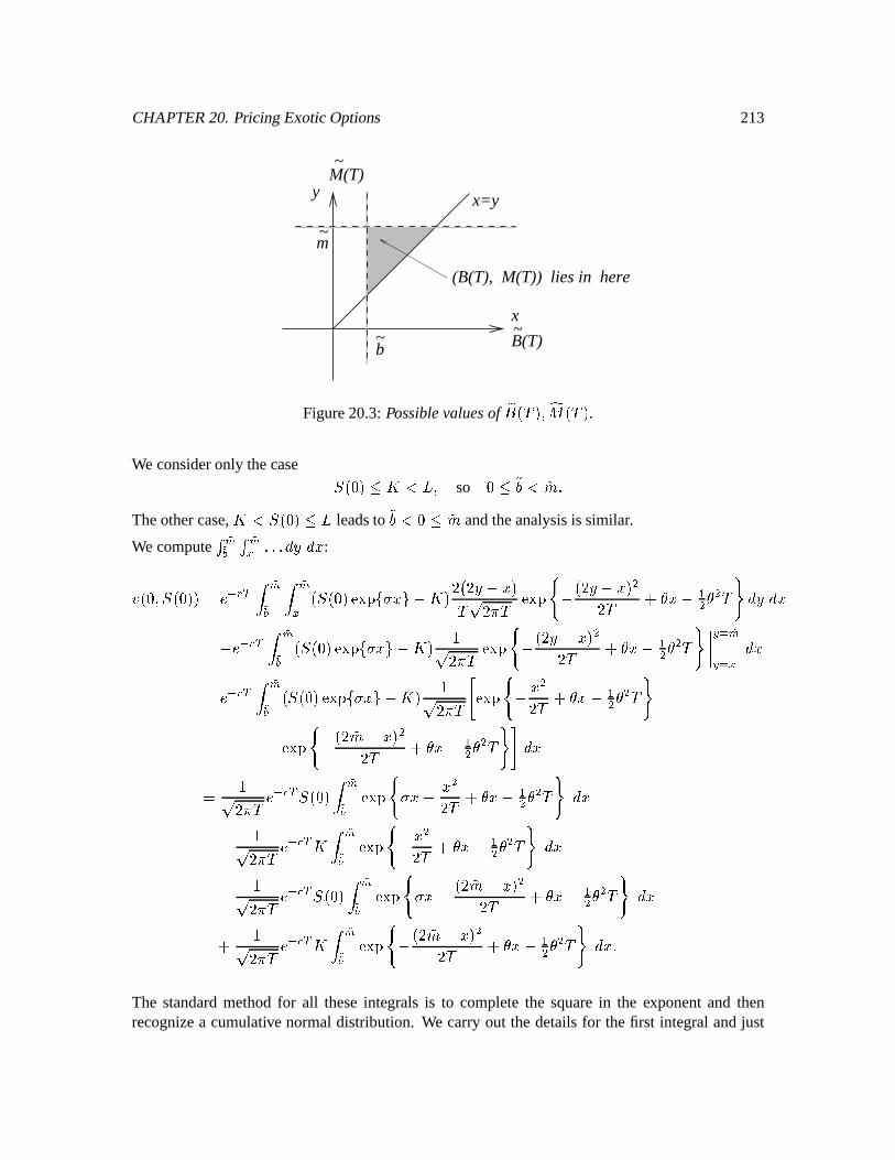
CHAPTER20. PricingExoticOptions 213
(B(T), M(T)) lies in here
M(T)
B(T)
x
y
b
m
~
~
~
~
x=y
Figure20.3:Possiblevaluesofþ® üÉÀ ÿ t ücÀ .
We consideronly thecase Ì ü ´ ãMÿso ! ã [
Theothercase,ã Ì ü leadsto ã g [ andtheanalysisis similar.
We computeË z Ë z .Xe! :¿ ü ÿ Ì ü wå æqç è z z ü Ì ü qÎEÏqÐ ! ¯ ´ ê ü ê ¯ À ô êë À ÎEÏqÐì ¯ ü ê ¯ ³ê À ý ¯ ³ ý ³ À ð ¯ å æqç è z ü Ì ü qÎEÏqÐ ! ¯ ´ éô êë À ÎEÏqÐì ¯ ü ê ¯ ³ê À ý ¯ ³ ý ³ À ð '''' ¡ V z¡ V
å æqç è z ü Ì ü <ÎEÏmÐ ! ¯ ´ éô êë À ÎEÏmÐ ì ¯ ³ê À ý ¯ ³ ý ³ À ð¯ ÎEÏqÐì ¯ ü ê [ ¯ ³ê À ý ¯ ³ ý ³ À ð éô êë À å æqç è Ì ü z ÎEÏmÐì ! ¯ ³ê À ý ¯ ³ ý ³ À ð
¯ éô êë À åæmç è ´ z ÎEÏmÐÂì ¯ ³ê À ý ¯ ³ ý ³ À ð ¯ éô êë À åæmç è Ì ü z ÎEÏmÐì ! ¯ ü ê [ ¯ ³ê À ý ¯ ³ ý ³ À ð éô êë À å æmç è ´ z ÎEÏmÐ ì ¯ ü ê [ ¯ ³ê À ý ¯ ³ ý ³ À ð 6
The standardmethodfor all theseintegrals is to completethe squarein the exponentand thenrecognizea cumulative normaldistribution. We carry out the detailsfor thefirst integral andjust
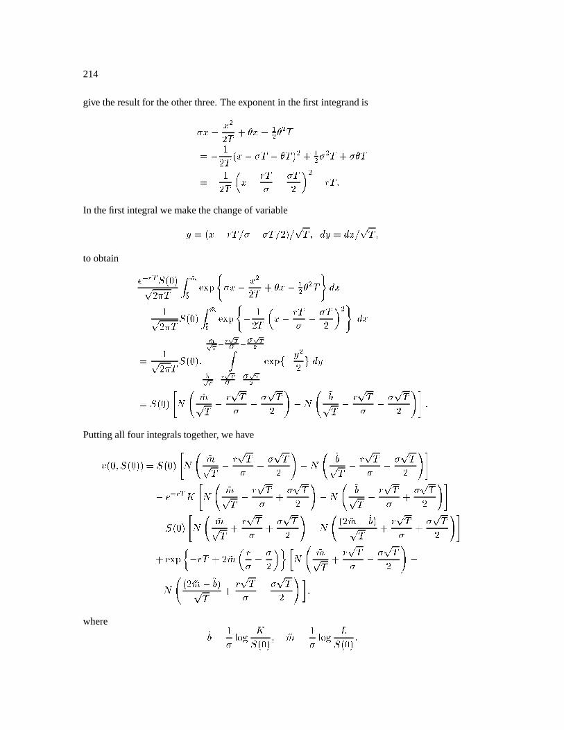
214
give theresultfor theotherthree.Theexponentin thefirst integrandis! ¯ ³ê À ý ¯ ³ ý ³ À ¯ éê À ü ¯ !wÀ ¯ ý À ³ ³ ! ³ ÀK! ý À ¯ éê À ¯ Í À! ¯ !Àê ¢ ³ Í À In thefirst integralwemakethechangeof variable ü ¯ Í À£¢2! ¯ !wÀ£¢ ê ¢ ô À ÿ ¢ ô À ÿto obtain å æqç è Ì ü ô êë À z ÎEÏmÐì ! ¯ ³ê À ý ¯ ³ ý ³ À ð éô ê¼ë À Ì ü z ÎEÏmÐÂì ¯ éê À ¯ Í À! ¯ !wÀê ¢ ³ð
éô ê¼ë À Ì ü :¤ ¥ æ¦ ¤ ¥! æ ! ¤ ¥g ¤ ¥ æ ¦ ¤ ¥! æ ! ¤ ¥g ÎEÏmÐ ¯ ³ê
Ì ü ó ? [ô À ¯ Í ô À! ¯ ! ô Àê D ¯ ó ? ô À ¯ Í ô À! ¯ ! ô Àê D Puttingall four integralstogether, wehave¿ ü ÿ Ì ü wÌ ü ó ? [ô À ¯ Í ô À! ¯ ! ô Àê D ¯ ó ? ô À ¯ Í ô À! ¯ ! ô Àê D ¯ å æmç è ´ ó ? [ô À ¯ Í ô À! ! ô Àê D ¯ ó ? ô À ¯ Í ô À! ! ô Àê D ¯ Ì ü ó ? [ô À Í ô À! ! ô Àê D ¯ ó ? ü ê [ ¯ ô À Í ô À! ! ô Àê D ÎEÏqÐ ^ ¯ Í À ê [ Í! ¯ ! ê ¢ h $ ó ? [ô À Í ô À! ¯ ! ô Àê D ¯
ó ? ü ê [ ¯ ô À Í ô À! ¯ ! ô Àê D * ÿwhere é! íAîï ´Ì ü ÿ [ é! íAîï Ì ü
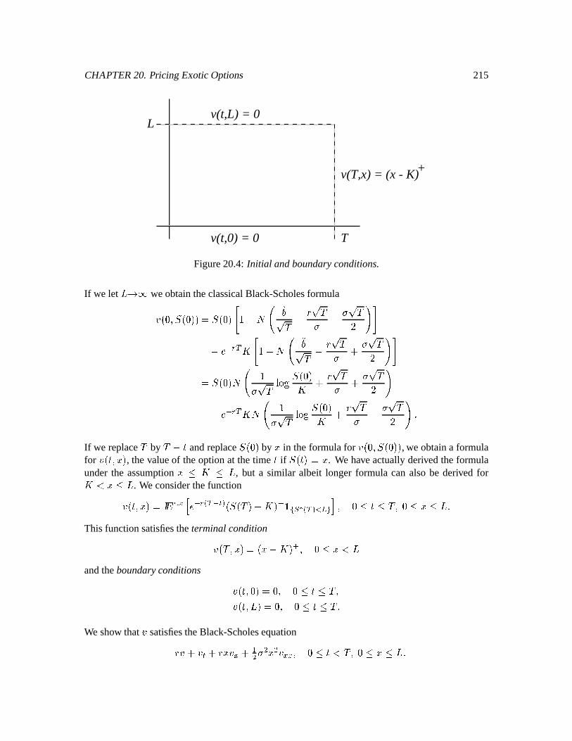
CHAPTER20. PricingExoticOptions 215
T
Lv(t,L) = 0
v(T,x) = (x - K)
v(t,0) = 0
+
Figure20.4: Initial andboundaryconditions.
If we let §©¨jª weobtaintheclassicalBlack-Scholesformula«+¬ e®¯°¬ 2±±²K¯°¬ 2±³ ´£µ·¶¹¸Gº»¼ ½ µ¿¾ ¼ ½À µ À ¼ ½Á ÂQõ·ÄÅeÆÇÉÈʳ˴̵Ͷ¸ º»¼ ½ µ ¾ ¼ ½À Î À ¼ ½Á ÂQòK¯°¬ 2±¶Ï¸ ´À ¼ ½jÐ-Ñ2Ò ¯°¬ Ó±È Î ¾ ¼ ½À Î À ¼ ½Á µ·Ä ÅeÆÇ ÈÔ¶ ¸ ´À ¼ ½jÐ-Ñ2Ò ¯Õ¬ 2±È Î ¾ ¼ ½À µ À ¼ ½Á ÂÍÖIf we replace
½by½ µÍ× andreplace°¬2± by Ø in theformulafor «+¬ e®\¯Õ¬ 2±J± , we obtaina formula
for «+¬B×® Ø ± , thevalueof theoptionat thetime × if ¯Õ¬B×˱Q² Ø . We have actuallyderivedtheformulaunderthe assumptionØÚÙ È ÙÛ§ , but a similar albeit longer formula can alsobe derived forÈGÜ ØÝÙ"§ . We considerthefunction«+¬B×\® Ø ±d²3Þ ßáà â ãáäåÄÅeÆæ4Ç0Åbà ¬ ¯Õ¬ ½ ±1µaÈÔ±JçdèeéJêë æ-Ç ìeíbîï ® Ù × Ù ½ ®ð Ù"ØÝÙ§ ÖThis functionsatisfiestheterminalcondition«+¬ ½ ® Ø ±1²ñ¬ Ø µ·ÈÔ± ç ® ÙØ Ü §andtheboundaryconditions «+¬B×®\2±ò²3e® Ù × Ù ½ ®«+¬B×® § ±ò²3e® Ù × Ù ½ ÖWe show that « satisfiestheBlack-Scholesequationµ ¾ « Î « à Îj¾ Ø « ã Î@óô À ô Ø ô « ãhã ® Ù ×QÜ ½ ®d ÙØõÙ§ Ö
216
Let ¯°¬ Ó±ö begivenanddefinethestoppingtime÷x²3øEùåúûü×Qýeþ©¯°¬B×±d² §Qÿ ÖTheorem 2.61 Theprocess Ä ÅeÆæ4à «+¬B×>÷®\¯°¬ ×õ÷e±J±h® Ù × Ù ½ ®is a martingale.
Proof: First notethat ¯2¬ ½ ±©Ü § ÷>ö ½ ÖLet begiven,andchoose× e® ½ . If ÷1¬ ± Ù × , thenÞ ß=Ä ÅeÆËÇ ¬ ¯°¬ ½ ±ÉµÍÈÔ± ç è éêë æ-Ç ìbíeî ¬B×±¬ ±Í² ÖBut when ÷1¬ ± Ù × , wehave«+¬B×>÷1¬ ±h®\¯Õ¬B×>÷1¬ ±h® ±J±d²3«+¬B×õ÷1¬ ±h® § ±É²3®sowemaywriteÞ ßBÄÅeÆÇ ¬ ¯Õ¬ ½ ±òµÍÈÔ±Jçdè éJê ë æ-Ç ìeíbî ¬ ×˱¬ ±Í²vÄÅeÆæ4à æ » «°¬B×Ý÷1¬ ±h®|¯Õ¬B×Ý÷1¬ ±h® ±± ÖOntheotherhand,if ÷1¬ ±Ìöj× , thentheMarkov propertyimpliesÞ ß Ä ÅeÆÇ ¬ ¯°¬ ½ ±1µaÈ ± ç èeéJêë æ-Ç ìeíbî ¬B×± ¬ ±²3Þ ß à â ê æ-à â ´ ä Ä ÅeÆÇ ¬ ¯Õ¬ ½ ±0µ·ÈÔ± ç è éJêë æ4Ç ìeíeîJï²3ÄÅeÆàË«+¬B×®\¯°¬ ×\® ±J±²3ÄÅeÆæ-à æ ´» «¬×>÷e®¯°¬ ×Ý÷1¬ ±h® ±J± ÖIn bothcases,wehaveÄÅeÆæ-à «+¬B×>÷e®\¯Õ¬B×õ÷e±J±d²3Þ ß ÄÅeÆÇ ¬ ¯Õ¬ ½ ±1µaÈÔ±Jçdè éJê ë æ-Ç ìeíbî ¬ ×˱ ÖSuppose Ù >Ù × Ù ½ . ThenÞ ß Ä ÅeÆ\æ-à «¬ ×>÷e®¯°¬B×!Ý÷e±J± ¬ ± ²3Þ ßBÞ ß=ÄÅeÆËÇQ¬ ¯°¬ ½ ±1µ·ÈÔ±Jçè éê ë æ-Ç ìbíeî ¬B×± ¬ ±"²3Þ ß Ä ÅeÆÇ ¬ ¯Õ¬ ½ ±1µaÈÔ± ç è éJêë æ-Ç ìeíbî ¬ ± ²3ÄÅbÆæ$#% «Õ¬ õ÷e®d¯°¬ õ÷e±J± Ö
CHAPTER20. PricingExoticOptions 217
For Ù × Ù ½ , wecomputethedifferential&(' ÄÅeÆàË«+¬B×®\¯°¬ ×˱J±*)²KÄÅeÆà\¬µ ¾ « Î « à ξ ¯©« ã Î óô À ô ¯ ô « ãhã ± & × Î ÄÅbÆà À+¯« ã &,+ ÖIntegratefrom to ×Ý÷ :Ä ÅeÆæ4à %- «¬å×>÷e®¯°¬B×>÷e±±d²3«¬e®\¯Õ¬ 2±J±Î . à / Ä ÅeÆ*# ¬µ ¾ « Î « à Îj¾ ¯« ã Î óô À ô ¯ ô « ãhã ± & Î . à / Ä ÅeÆ*# À1¯« ã &0+ Ö1 243 5
A stoppedmartingaleis still amartingale
BecauseÄ ÅbÆæ-à %- «°¬B×>÷e®\¯Õ¬B×>÷e±J± is alsoa martingale,theRiemannintegral. à / Ä ÅeÆ"# ¬µ ¾ « Î « à Îj¾ ¯« ã Î@óô À ô ¯ ô « ãhã ± & is amartingale.Therefore,µ ¾ «¬ ®\¯Õ¬ ±± Î « à ¬ ®\¯°¬ ±J± Îa¾ ¯°¬ ±J« ã ¬ ®\¯°¬ ±J± Î óô À ô ¯ ô ¬ ±« ãhã ¬ ®¯°¬ ±J±1²3® Ù6õÙ ×>÷ ÖThePDE µ ¾ « Î « à ξ Ø « ã Î óô À ô Ø ô « ãhã ²3e® Ù × Ù ½ ®d ÙØõÙ§ ®thenfollows.
The Hedge & ' Ä ÅeÆà «¬B×®\¯Õ¬B×˱J± ) ²3Ä ÅbÆà À1¯Õ¬B×˱« ã ¬B×\®¯°¬B×±J± &0+ ¬B×˱h® Ù × Ù ÷ ÖLet 7 ¬B×˱ bethewealthprocesscorrespondingto someportfolio 8 ¬B×˱ . Then& ¬ Ä ÅeÆà 7 ¬B×˱J±ò²3Ä ÅbÆà 8 ¬ ×˱JÀ+¯°¬ ×˱ &,+ ¬B×± ÖWe shouldtake 7 ¬ 2±ò²3«+¬ e®\¯Õ¬ 2±J±and 8 ¬B×˱d²K« ã ¬B×®\¯Õ¬B×˱J±i® Ù × Ù ½ >÷ ÖThen 7 ¬ ½ >÷e±²K«¬ ½ >÷e®¯°¬ ½ Ý÷e±J±²:9 «¬ ½ ®\¯Õ¬ ½ ±J±+²ñ¬¯°¬ ½ ±òµÍÈÔ± ç if ÷>ö ½«¬÷e® § ±1²3 if ÷ Ù ½ .
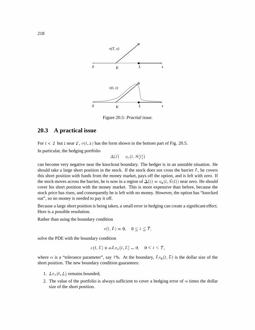
218
K L x
v(T, x)
0
0 K L x
v(t, x)
Figure20.5:Practial issue.
20.3 A practical issue
For × Ü ½ but × near½
, «¬ ×\® Ø ± hastheform shown in thebottompartof Fig. 20.5.
In particular, thehedgingportfolio 8 ¬B×˱d²3« ã ¬B×®\¯°¬ ×˱J±canbecomevery negative neartheknockoutboundary. Thehedgeris in anunstablesituation.Heshouldtakea largeshortpositionin thestock. If thestockdoesnot crossthebarrier § , hecoversthis shortpositionwith fundsfrom themoney market,paysoff theoption,andis left with zero. Ifthestockmovesacrossthebarrier, heis now in aregionof 8 ¬B×˱©²3« ã ¬B×®\¯Õ¬B×˱J± nearzero.Heshouldcover his shortpositionwith themoney market. This is moreexpensive thanbefore,becausethestockpricehasrisen,andconsequentlyheis left with nomoney. However, theoptionhas“knockedout”, sonomoney is neededto payit off.
Becausealargeshortpositionis beingtaken,asmallerrorin hedgingcancreateasignificanteffect.Hereis a possibleresolution.
Ratherthanusingtheboundarycondition«+¬B×® § ±ò²3e® Ù × Ù ½ ®solve thePDEwith theboundarycondition«¬B×® § ± Î<; § « ã ¬ ×\® § ±É²Ke® Ù × Ù ½ ®where ; is a “toleranceparameter”,say ´ %. At the boundary, § « ã ¬B×® § ± is the dollar sizeof theshortposition.Thenew boundaryconditionguarantees:
1. § « ã ¬B×\® § ± remainsbounded;
2. Thevalueof theportfolio is alwayssufficient to cover a hedgingerrorof ; timesthedollarsizeof theshortposition.
Chapter 21
Asian Options
Stock: & ¯Õ¬B×˱ò² ¾ ¯°¬ ×˱ & × Î À+¯Õ¬B×˱ &,+ ¬B×± ÖPayoff: = ²?>Ô¸ . Ç/ ¯Õ¬B×˱ & × ÂValueof thepayoff at timezero:7 ¬ 2±ò²3Þ ß ³ Ä ÅeÆÇ > ¸ . Ç/ ¯°¬ ×˱ & × ÂQà ÖIntroduceanauxiliary process@ ¬B×± by specifying& @ ¬ ×˱²K¯°¬B×± & × ÖWith theinitial conditions ¯°¬ ×˱d² Ø ® @ ¬ ×˱d²?A®wehave thesolutions¯°¬ ½ ±ò² ØCBEDFHG À©¬ + ¬ ½ ±dµ + ¬B×±J± Î ¬ ¾ µ óô À ô ±ü¬ ½ µÍ×±EI®@ ¬ ½ ±d²?A Î . Çà ¯°¬ ± & ÖDefinetheundiscountedexpectedpayoff ¬ ×\® Ø ®JA±É²KÞ ß à â ãâ K >ɬ @ ¬ ½ ±J±i® Ù × Ù ½ ® Ø ý"e®LA Þ M Ö
219
220
21.1 Feynman-KacTheorem
Thefunction satisfiesthePDE à Îj¾ ØN ã Î@óô À ô Ø ô ãhã Î Ø K ²3e® Ù × Ù ½ ® Ø ý®OA Þ ME®theterminalcondition ¬ ½ ® Ø ®4A/±0²?>ɬPA±h® Ø ýe®LA Þ ME®andtheboundarycondition ¬B×®\e®4A/±ò²?>ò¬PA/±i® Ù × Ù ½ ®LA Þ M ÖOnecansolvethisequation.Then «(QÓ×\®¯°¬B×±h® . à/ ¯°¬ ± & !Ris theoptionvalueat time × , where«+¬B×® Ø ®4A/±ò²TÄ ÅeÆæ4Ç0Åeà - ¬B×\® Ø ®JA± ÖThePDEfor « is µ ¾ « Î « à ξ Ø « ã Î óô À ô Ø ô « ãhã Î Ø « K ²3® (1.1)«¬ ½ ® Ø ®JA±+²?>ɬPA±h®«¬B×®\e®4A/±0²3ÄÅeÆæ4Ç0Åeà - >ò¬PA/± ÖOnecansolvethisequationratherthantheequationfor .21.2 Constructing the hedge
Startwith thestockprice ¯Õ¬ 2± . Thedifferentialof thevalue 7 ¬ ×˱ of aportfolio 8 ¬B×± is& 7 ² 8 & ¯ Î"¾ ¬ 7 µ 8 ¯©± & ײ 8 ¯Õ¬ ¾ & × Î À &,+ ± Îj¾ 7 & ×òµ ¾ 8 ¯ & ײ 8 À0¯ &0+ ξ 7 & × ÖWe wantto have 7 ¬B×˱ò²3«SQ×\®¯°¬B×±h® . à/ ¯Õ¬ ± & !R ®sothat 7 ¬ ½ ±ò²3«>¸ ½ ®¯°¬ 2±i® . Ç/ ¯Õ¬ ± &  ®²?> ¸ . Ç/ ¯°¬ ± & ÂÍÖ
CHAPTER21. AsianOptions 221
Thedifferentialof thevalueof theoptionis& «TQ2×\®¯°¬B×±h® . à/ ¯Õ¬ ± & !R ²3« à & × Î « ã & ¯ Î « K ¯ & × Î óô « ãhã & ¯ & ¯²ñ¬ « à Îj¾ ¯« ã Î ¯« K Î óô À ô ¯ ô « ãhã ± & × Î À1¯« ã &0+² ¾ «+¬B×\®¯°¬B×±J± & × Î « ã ¬B×®\¯°¬ ×˱J±òÀ>¯°¬B×± &0+ ¬B×˱ Ö (FromEq. 1.1)
Comparethiswith & 7 ¬B×˱ò² ¾ 7 ¬B×˱ & × Î 8 ¬B×˱©À>¯°¬B×± &0+ ¬B×˱ ÖTake 8 ¬ ×˱d²3« ã ¬B×\®¯°¬B×±J± Ö If 7 ¬ 2±ò²3«¬e®\¯Õ¬ 2±h®J2± , then7 ¬B×˱ò²3« Q ×\®¯°¬B×±h® . à/ ¯Õ¬ ± & R ® Ù × Ù ½ ®becauseboththeseprocessessatisfythesamestochasticdifferentialequation,startingfromthesameinitial condition.
21.3 Partial averagepayoff Asian option
Now supposethepayoff is = ²?>Ô¸ . Ç ¯Õ¬B×˱ & × Â ®wherexÜ÷ Ü ½ . We compute«+¬ ÷e® Ø ®4A/±+²3Þ ß â ãâ K Ä ÅeÆ\æ-Ç1Å %- >ò¬ @ ¬ ½ ±J±justasbefore.For Ù × Ù ÷ , wecomputenext thevalueof aderivativesecuritywhichpaysoff«¬÷e®\¯Õ¬ ÷e±h®J2±at time ÷ . Thisvalueis U ¬B×\® Ø ±ò²3Þ ßáà â ãÄÅeÆæ Åeà - «¬ ÷®\¯°¬÷e±h®J2± ÖThefunction
UsatisfiestheBlack-ScholesPDEµ ¾ U Î U à Îj¾ Ø U ã Î óô À ô Ø ô U ãhã ²3e® Ù × Ù ÷e® Ø ý"e®
with terminalcondition U ¬÷e® Ø ±1²3«+¬ ÷e® Ø ®\2±i® Ø ýe®andboundarycondition U ¬B×®\2±ò²3ÄÅbÆæ-Ç1Åeà - >ò¬ 2±h® Ù × Ù ½ ÖThehedgeis givenby 8 ¬ ×˱²WVX Y U ã ¬B×®\¯°¬ ×˱J±h® Ù × Ù ÷®« ã ' ×\®¯°¬B×±h®JZ à ¯Õ¬ ± & ) ® ÷ Üj× Ù ½ Ö
222
Remark 21.1 While noclosed-formfor theAsianoptionpriceis known, theLaplacetransform(inthe variable
À[\ ¬ ½ µa×˱ ) hasbeencomputed.SeeH. GemanandM. Yor, Besselprocesses,Asianoptions,andperpetuities,Math. Finance3 (1993),349–375.
Chapter 22
Summary of Arbitrage Pricing Theory
A simpleEuropeanderivativesecuritymakesa randompaymentat a time fixed in advance.Thevalueat time × of sucha securityis theamountof wealthneededat time × in orderto replicatethesecurityby tradingin themarket.Thehedgingportfolio is a specificationof how to do this trading.
22.1 Binomial model,HedgingPortf olio
Let bethesetof all possiblesequencesof ] coin-tosses.We have no probabilitiesat this point.Let ¾ ý"e® ö ¾Î ´2® & ²Ú´%^ begiven.(SeeFig. 2.1)
Evolutionof thevalueof aportfolio:7`_ ç ó ² 8(_ ¯ _ ç ó Î ¬´ ξ ±ü¬ 7`_ µ 8a_ ¯ _ ± ÖGivenasimpleEuropeanderivativesecurity
= ¬ ó ® ô ± , wewantto startwith anonrandom7 / anduseaportfolio processes 8 / ® 8 ó ¬cb ±i® 8 ó ¬ ½ ±sothat 7 ô ¬ ó ® ô ±d² = ¬ ó ® ô ±ed ó ® ô Ö (four equations)
Therearefour unknowns: 7 / ® 8 / ® 8 ó ¬PbÔ±h® 8 ó ¬ ½ ± . Solvingtheequations,weobtain:
223
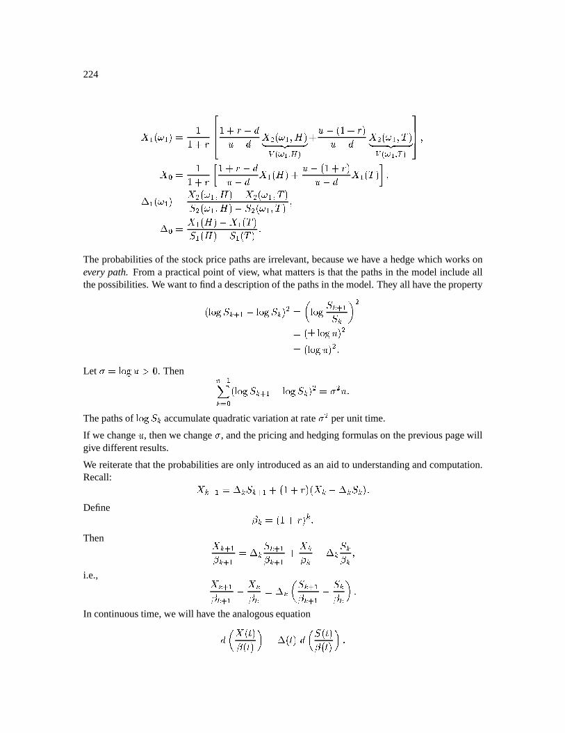
224
7 ó ¬ ó ±d² ´´ ξgfhhi ´ ξ µ & µ & 7 ô ¬ ó ®4bÔ±1 243 5j æ lk â m - Î µ¬´ ξ ± µ & 7 ô ¬ ó ® ½ ±1 243 5j æ nk â Ç -oqppr ®7 / ² ´´ ξ ´ Îj¾ µ & µ & 7 ó ¬PbÔ± Î µ¬´ Îj¾ ± µ & 7 ó ¬ ½ ±£®8 ó ¬ ó ±d² 7 ô ¬ ó ®JbÔ±1µ 7 ô ¬ ó ® ½ ±¯ ô ¬ ó ®JbÔ±1µa¯ ô ¬ ó ® ½ ± ®8 / ² 7 ó ¬PbÔ±òµ 7 ó ¬ ½ ±¯ ó ¬PbÔ±òµÍ¯ ó ¬ ½ ± Ö
Theprobabilitiesof thestockpricepathsareirrelevant,becausewe have a hedgewhich worksoneverypath. Froma practicalpoint of view, whatmattersis that thepathsin themodelincludeallthepossibilities.Wewantto find adescriptionof thepathsin themodel.They all have theproperty¬ Ð-Ñ2Ò ¯ _ ç ó µ Ð-Ñ2Ò ¯ _ ± ô ²sQ Ð-Ñ2Ò ¯ _ ç ó¯ _ R ô²@¬Pt Ð-Ñ2Ò ± ô²@¬ Ð-Ñ2Ò ± ô ÖLet À>² Ð-Ñ2Ò ö . Then u Å óv_4w / ¬ Ð4ÑÓÒ ¯ _ ç ó µ Ð-Ñ2Ò ¯ _ ± ô ²3À ô ] ÖThepathsof Ð4ÑÓÒ ¯ _ accumulatequadraticvariationat rate À ô perunit time.
If we change , thenwe changeÀ , andthepricing andhedgingformulason thepreviouspagewillgivedifferentresults.
We reiteratethattheprobabilitiesareonly introducedasanaid to understandingandcomputation.Recall: 7`_ ç ó ² 8(_ ¯ _ ç ó Î ¬´ ξ ±ü¬ 7`_ µ 8a_ ¯ _ ± ÖDefine x _ ²@¬´ Îj¾ ± _ ÖThen 7`_ ç óx _ ç ó ² 8(_ ¯ _ ç óx _ ç ó Î 7`_x _ µ 8(_ ¯ _x _ ®i.e., 7`_ ç óx _ ç ó µ 7S_x _ ² 8a_ Q ¯ _ ç óx _ ç ó µ ¯ _x _ R ÖIn continuoustime,wewill have theanalogousequation& Q 7 ¬B×˱x ¬B×± R ² 8 ¬B×˱ & Q ¯Õ¬B×˱x ¬B×˱ R Ö
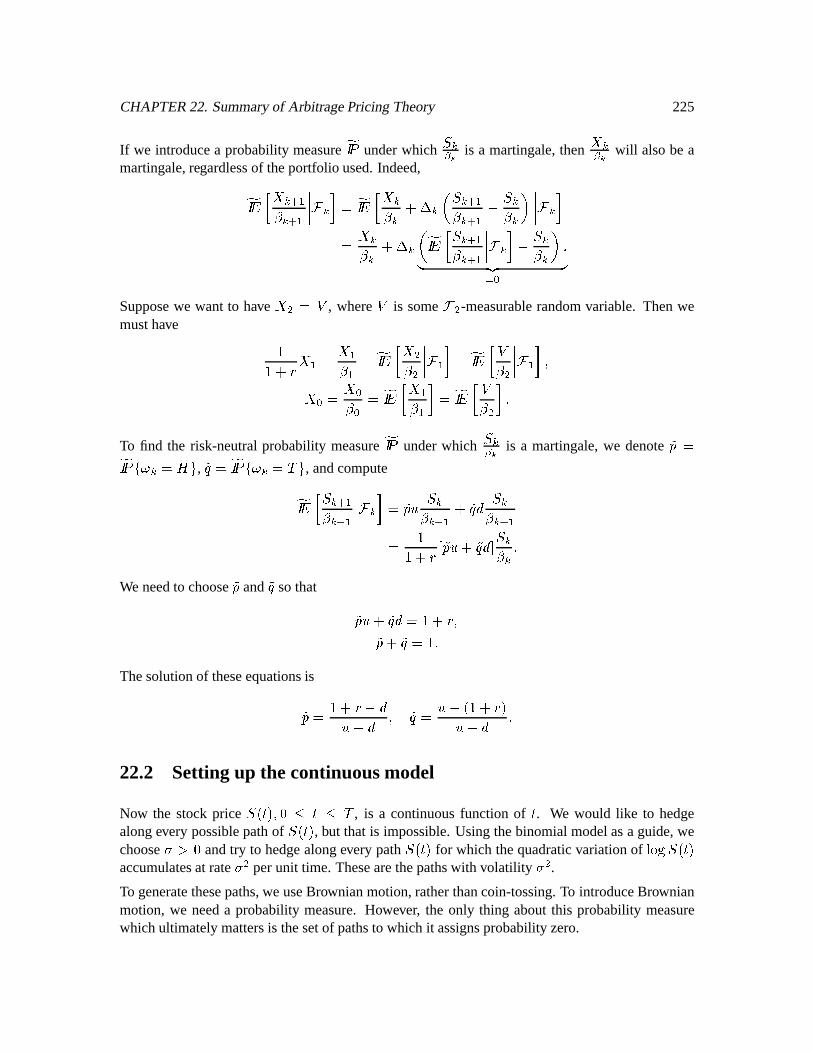
CHAPTER22. Summaryof ArbitragePricingTheory 225
If we introducea probabilitymeasurey Þ z underwhich¯ _%| is a martingale,then 7`_%| will alsobea
martingale,regardlessof theportfolio used.Indeed,y Þ ß 7`_ ç óx _ ç ó _ ² y Þ ß 7S_x _ Î 8(_ Q ¯ _ ç óx _ ç ó µ ¯ _x _ R _ ² 7`_x _ Î 8a_ Q yÞ ß ¯ _ ç óx _ ç ó _ µ ¯ _x _ R Ö1 2J3 5w /Supposewe want to have 7 ô ² = , where
=is some ô -measurablerandomvariable. Thenwe
musthave ´´ Îj¾ 7 ó ² 7 óx ó ² y Þ ß 7 ôx ô ó ² yÞ ß =x ô ó ®7 / ² 7 /x / ² yÞ ß 7 óx ó ² yÞ ß
=x ô ÖTo find the risk-neutralprobability measurey Þ z underwhich
¯ _ | is a martingale,we denote ºT²y Þ z û l_ ²~b ÿ , º² y Þ z û O_ ² ½ ÿ , andcomputey Þ ß ¯ _ ç óx _ ç ó _ ² º ¯ _x _ ç ó Î º & ¯ _x _ ç ó² ´´ Îj¾ º Î º & ¯ _x _ ÖWe needto chooseº and º sothat º Î º & ²q´ ξ ®º Î º²q´ ÖThesolutionof theseequationsisºx² ´ Î"¾ µ & µ & ® º² µ¬´ Îj¾ ± µ & Ö22.2 Settingup the continuousmodel
Now the stock price ¯Õ¬B×˱h® Ù × Ù ½ , is a continuousfunction of × . We would like to hedgealongevery possiblepathof ¯°¬B×± , but that is impossible.Usingthebinomialmodelasa guide,wechooseÀ·ö andtry to hedgealongevery path ¯°¬B×± for which thequadraticvariationof Ð-Ñ2Ò ¯Õ¬B×˱accumulatesat rate À ô perunit time. Thesearethepathswith volatility À ô .To generatethesepaths,we useBrownianmotion,ratherthancoin-tossing.To introduceBrownianmotion, we needa probability measure.However, the only thing aboutthis probability measurewhichultimatelymattersis thesetof pathsto which it assignsprobabilityzero.
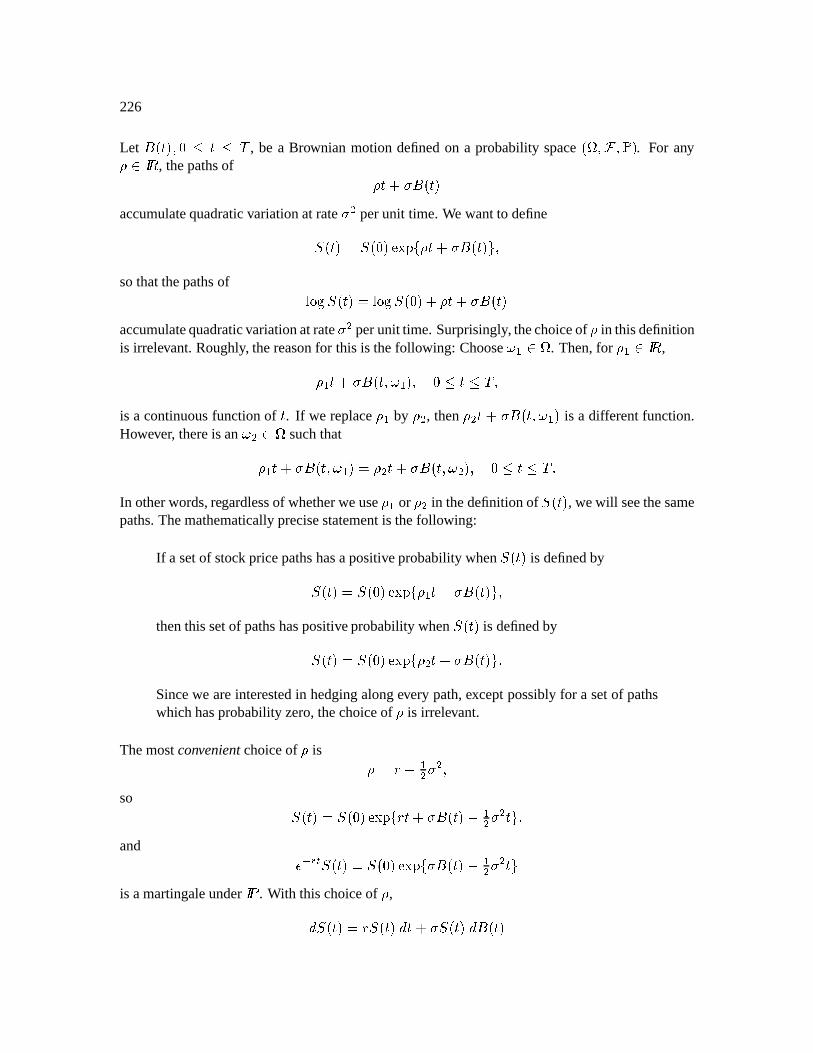
226
Let+ ¬B×˱ ®\ Ù × Ù ½ , be a Brownian motion definedon a probability space¬ ® ®± . For any Þ M , thepathsof /× Î À + ¬B×±
accumulatequadraticvariationat rate À ô perunit time. We wantto define¯Õ¬B×˱d²K¯°¬ 2± BEDF û%/× Î À + ¬ ×˱ ÿ ®sothatthepathsof Ð4ÑÓÒ ¯Õ¬B×˱d² Ð4ÑÓÒ ¯°¬2± Î /× Î À + ¬B×±accumulatequadraticvariationatrateÀ ô perunit time. Surprisingly, thechoiceof in thisdefinitionis irrelevant.Roughly, thereasonfor this is thefollowing: Choose ó . Then,for ó Þ M , ó × Î À + ¬B×\® ó ±h® Ù × Ù ½ ®is a continuousfunctionof × . If we replace ó by ô , then ô × Î À + ¬B×\® ó ± is a differentfunction.However, thereis an ô suchthat ó × Î À + ¬B×® ó ±d²~ ô × Î À + ¬B×® ô ±h® Ù × Ù ½ ÖIn otherwords,regardlessof whetherweuse ó or ô in thedefinitionof ¯°¬B×± , wewill seethesamepaths.Themathematicallyprecisestatementis thefollowing:
If a setof stockpricepathshasapositiveprobabilitywhen ¯°¬B×± is definedby¯Õ¬B×˱d²K¯°¬ 2± BEDF û% ó × Î À + ¬ ×˱ ÿ ®thenthissetof pathshaspositiveprobabilitywhen ¯°¬ ×˱ is definedby¯Õ¬B×˱d²K¯°¬ 2± BEDF û% ô × Î À + ¬ ×˱ ÿ ÖSincewe areinterestedin hedgingalongevery path,exceptpossiblyfor a setof pathswhichhasprobabilityzero,thechoiceof is irrelevant.
Themostconvenientchoiceof is E² ¾ µ óô À ô ®so ¯Õ¬B×˱d²3¯Õ¬ 2± BEDF û ¾ × Î À + ¬B×˱©µ óô À ô × ÿ ®and ÄÅeÆË௰¬B×±d²3¯°¬2± BED!F ûCÀ + ¬ ×˱©µ óô À ô × ÿis amartingaleunder Þ z . With thischoiceof ,& ¯°¬B×±d² ¾ ¯°¬B×± & × Î À1¯°¬ ×˱ &,+ ¬B×±
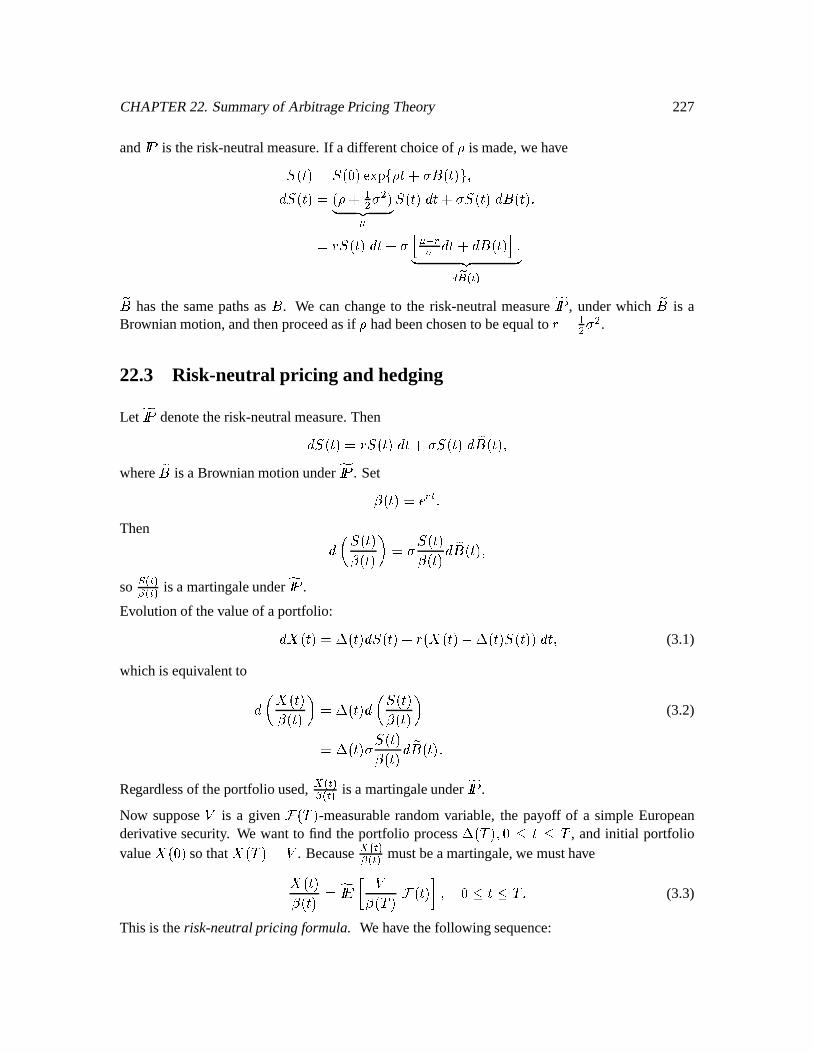
CHAPTER22. Summaryof ArbitragePricingTheory 227
and Þ z is therisk-neutralmeasure.If a differentchoiceof is made,wehave¯Õ¬B×˱d²3¯Õ¬ 2± BEDF û/× Î À + ¬B×± ÿ ®& ¯Õ¬B×˱d²ñ¬ Î óô À ô ±1 243 5 ¯Õ¬B×˱ & × Î À1¯Õ¬B×˱ &,+ ¬ ×˱ Ö² ¾ ¯Õ¬B×˱ & × Î À ä ÅbÆ & × Î &0+ ¬B×˱ ï Ö1 2J3 5 æ-à -+hasthe samepathsas
+. We canchangeto the risk-neutralmeasurey Þ z , underwhich
+is a
Brownianmotion,andthenproceedasif hadbeenchosento beequalto ¾ µ óô À ô .22.3 Risk-neutral pricing and hedging
Let y Þ z denotetherisk-neutralmeasure.Then& ¯Õ¬B×˱ò² ¾ ¯°¬ ×˱ & × Î À+¯Õ¬B×˱ & + ¬B×˱h®where
+is a Brownianmotionundery Þ z . Setx ¬B×±²TÄhÆà Ö
Then & Q ¯°¬B×±x ¬ ×˱ R ²3À ¯Õ¬B×˱x ¬B×˱ & + ¬ ×˱h®soê æ-à - æ-à - is a martingaleundery Þ z .
Evolutionof thevalueof aportfolio:& 7 ¬ ×˱ò² 8 ¬B×± & ¯Õ¬B×˱ Îj¾ ¬ 7 ¬Bױɵ 8 ¬B×˱J¯Õ¬B×˱± & ×\® (3.1)
which is equivalentto & Q 7 ¬B×±x ¬B×± R ² 8 ¬B×± & Q ¯°¬B×±x ¬B×± R (3.2)² 8 ¬B×±JÀ ¯°¬B×±x ¬B×± & + ¬B×˱ ÖRegardlessof theportfolio used, æ-à - æ-à - is a martingaleundery Þ z .
Now suppose
=is a given ¬ ½ ± -measurablerandomvariable,the payoff of a simpleEuropean
derivative security. We want to find the portfolio process8 ¬ ½ ±i®\ Ù × Ù ½ , andinitial portfoliovalue 7 ¬2± sothat 7 ¬ ½ ±É² = . Because æ-à - æ-à - mustbeamartingale,we musthave7 ¬B×˱x ¬B×˱ ² yÞ ß =x ¬ ½ ± ¬B×˱ ® Ù × Ù ½ Ö (3.3)
This is therisk-neutral pricing formula. We have thefollowing sequence:
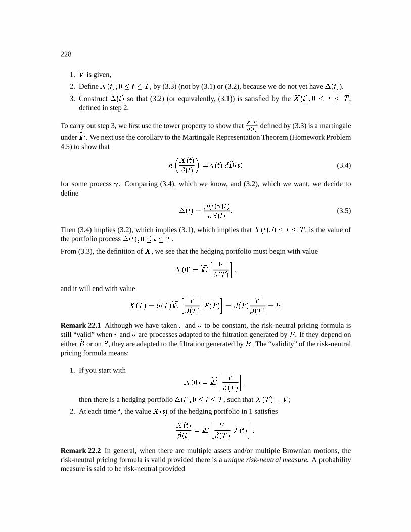
228
1.
=is given,
2. Define 7 ¬B×±h®\ Ù × Ù ½ , by (3.3) (notby (3.1)or (3.2),becausewedonotyethave 8 ¬ ×˱ ).3. Construct8 ¬B×± so that (3.2) (or equivalently, (3.1)) is satisfiedby the 7 ¬B×±h®\ Ù × Ù ½ ,
definedin step2.
To carryoutstep3, wefirst usethetowerpropertyto show that æ4à - æ4à - definedby (3.3)is amartingale
undery Þ z . Wenext usethecorollaryto theMartingaleRepresentationTheorem(HomeworkProblem4.5)to show that & Q 7 ¬B×˱x ¬B×˱ R ²~¬B×˱ & + ¬B×± (3.4)
for someproecss . Comparing(3.4), which we know, and(3.2), which we want, we decidetodefine 8 ¬B×±d² x ¬B×±*¬B×˱À¯Õ¬B×˱ Ö (3.5)
Then(3.4) implies(3.2),which implies(3.1),which impliesthat 7 ¬B×±h®\ Ù × Ù ½ , is thevalueoftheportfolio process8 ¬B×±h®\ Ù × Ù ½ .
From(3.3),thedefinitionof 7 , we seethatthehedgingportfolio mustbegin with value7 ¬2±É² y Þ ß =x ¬ ½ ± ®andit will endwith value7 ¬ ½ ±ò² x ¬ ½ ± yÞ ß =x ¬ ½ ± ¬ ½ ±c ² x ¬ ½ ±
=x ¬ ½ ± ² = ÖRemark 22.1 Althoughwe have taken ¾ and À to beconstant,the risk-neutralpricing formula isstill “valid” when ¾ and À areprocessesadaptedto thefiltration generatedby
+. If they dependon
either+
or on ¯ , they areadaptedto thefiltration generatedby+
. The“validity” of therisk-neutralpricing formulameans:
1. If you startwith 7 ¬ ӱɲ y Þ ß =x ¬ ½ ± £®thenthereis a hedgingportfolio 8 ¬B×±h®\ Ù × Ù ½ , suchthat 7 ¬ ½ ±ò² = ;
2. At eachtime × , thevalue 7 ¬B×˱ of thehedgingportfolio in 1 satisfies7 ¬B×˱x ¬B×˱ ² yÞ ß =x ¬ ½ ± ¬B×˱ ÖRemark 22.2 In general,when therearemultiple assetsand/ormultiple Brownian motions,therisk-neutralpricing formulais valid providedthereis a uniquerisk-neutral measure. A probabilitymeasureis saidto berisk-neutralprovided
CHAPTER22. Summaryof ArbitragePricingTheory 229 it hasthesameprobability-zerosetsastheoriginalmeasure; it makesall thediscountedassetpricesbemartingales.
To seeif therisk-neutralmeasureis unique,computethedifferentialof all discountedassetpricesandcheckif thereis morethanoneway to define
+so that all thesedifferentialshave only
& +terms.
22.4 Implementation of risk-neutral pricing and hedging
To geta computableresultfrom thegeneralrisk-neutralpricing formula7 ¬B×±x ¬ ×˱ ² yÞ ß =x ¬ ½ ± ¬ ×˱ ®oneusestheMarkov property. Weneedto identifysomestatevariables,thestockpriceandpossiblyothervariables,sothat 7 ¬Bױɲ x ¬B×˱ yÞ ß =x ¬ ½ ± ¬ ×˱ is a functionof thesevariables.
Example22.1 Assume and areconstant,and <<O . We cantakethestockpriceto bethestatevariable.Define $J*0 ¡£¢P¤ ¥ ä$¦¨§0©ª¬«§ ¢ ®¯O ïO°Then ± ²" ¦ © ¢ ¡ ¦ §0©c« O ´³ ²" $J*®$"µand ¶ ª ¢· ª ¢ ¦ §,© ¢ ²J"®²" is a martingaleunder
¸.
Example22.2 Assume and areconstant.¹ ¸ . «º ®»,¼½»  °Take ®$" and ¾T$" Z ¢º ®»0¼½» to bethestatevariables.Define $J**¿%À ¡C¢P¤ ¥%¤ Á 䦨§0©µª´«§ ¢ ¾Ã¯O ï where ¾ÃO¹¿Ä . «¢ ®»,¼½» °
230
Then ± $"® ¦ © ¢ ¡ ¦ §,©P« N®¯O ³ $" ²J"®²"¾($"and
± ²"Å $" ¦ §0© ¢ ²J"®$"µ¾(²"is a martingaleunder
¸.
Example22.3 (Homework problem4.2)¼Æ®²"ǽ²J¾È$"À²"¼¨ÄÉ$J¾Ã$"®$"®¼ Ê $"µ¼¾Ã$"À¹Ë®$J¾Ì$"¼¨ÍÄÏβJ¾Ã²"¼ Ê ²"¹ÇN®¯O °Take ®$" and ¾T$" to bethestatevariables.Define ²J"N*¿% ¡ ¢P¤ ¥¤ Á fhhhhhhiPÐÑ½Ò 9Ó . «¢ ½»¾Ì»,¼½»Ô1 243 5ÕµÖ ×$ØÕÖ ÙÆØ ®¯O oqppppppr °Then ± $" Å $" ¡ OÅ ¯O ³ ²" ¡ ³ ÐÑ½Ò 9Ó . «¢ ½»¾Ã»0¼½»ÔÈ®¯O ³ ²" à ²J"®$"µ¾T$"and
± $"Å ²" ÐѽÒÚ Ó . ¢º ½»¾Ì»,¼½»Û $J*®$"µ¾T$"
is a martingaleunder ¸
.
In every case,we get an expressioninvolving « to be a martingale.We takethe differentialandsetthe
& × term to zero. This givesus a partial differentialequationfor « , andthis equationmusthold wherever the stateprocessescanbe. The
&£+term in the differentialof the equationis the
differentialof a martingale,andsincethemartingaleis7 ¬ ×˱x ¬B×˱ ² 7 ¬ 2± Î . à/ 8 ¬ ±JÀ ¯Õ¬ ±x ¬ ± & + ¬ ±wecansolvefor 8 ¬B×± . This is theargumentwhichuses(3.4)to obtain(3.5).
CHAPTER22. Summaryof ArbitragePricingTheory 231
Example22.4(Continuation of Example22.3)± $"Å $" ÐѽÒÚ Ó . ¢º ½»N¾Ì»0¼½»Û1 243 5ÜÝ · ª ¢ $J*®$"¾T$"
is a martingaleunder ¸
. Wehave¼ Q ± $"Å $" R ÞÅ ²" Ó ½$J¾Ã²" $J*®$"¾($"¼¨Ä ¢ ¼¨Ä ¥ ¼½TÄ Á ¼¾Ä Üß ¥4¥ ¼½S¼½Ä ¥JÁ ¼½S¼à¾Ä Üß ÁÁ ¼¾á¼¾ ÞÅ ²" Ó Ä ¢ ÄÏE ¥ ÄÉË Á Ä Üß ß ß ¥4¥ ÄÉ,Î0 ¥JÁ Ä Üß Î ß ÁÁ ¼¨Ä! ¥ ÄÎ Á ¼ Ê Thepartialdifferentialequationsatisfiedby
isÓ Ä ¢ ÄÏE ¥ ÄÉË Á Ä Üß ß ß ¥4¥ Ä!Î, ¥4Á Ä Üß Î ß ÁÁ â
whereit shouldbenotedthat $J**¿% , andall othervariablesarefunctionsof ²J"¿ . We have¼ Q ± ²"Å $" R ÞÅ $",ã ! ¥ ÄäÎ ÁEå ¼ Ê ²"
where T<$J¾Ã$" , ÎTÎ$J¾Ã²" , $J*®$"¾T$" , and <²" . We wantto chooseæT²" sothat(see(3.2)) ¼ Q ± $"Å ²" R ¹æT²"$J¾Ã²" ®²"Å $" ¼ Ê ²" °Therefore,weshouldtake æT²" to beæT²" ¥ $J*²"¾Ã$"Ä Î$J¾Ã$"$J¾Ã²"®$" Á ²J"®$"µ¾È$" °

232
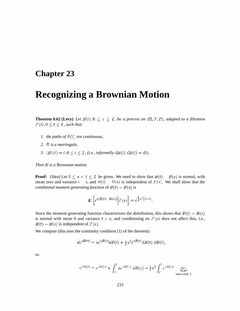
Chapter 23
Recognizinga Brownian Motion
Theorem 0.62(Levy) Let+ ¬B×˱ ®\ Ù × Ù ½ ® be a processon ¬ ® ®± , adaptedto a filtration ¬B×˱i®\ Ù × Ù ½ , such that:
1. thepathsof+ ¬B×± arecontinuous,
2.+
is a martingale,
3. ç +Ãè ¬ ×˱d²T×®\ Ù × Ù ½ , (i.e., informally&0+ ¬B×˱ &0+ ¬B×˱©² & × ).
Then+
is a Brownianmotion.
Proof: (Idea)Let Ù:é Ü× Ù ½ begiven. We needto show that+ ¬B×˱̵ + ¬ é ± is normal,with
meanzeroandvariance×Qµ é , and+ ¬B×˱̵ + ¬ é ± is independentof ¬ é ± . We shall show that the
conditionalmomentgeneratingfunctionof+ ¬ ×˱©µ + ¬ é ± isÞ ß ÄE#æ æ4à - Å æ¯ê -- ¬ é ± ²KÄ óô # [ æ-à Åê - Ö
Sincethemomentgeneratingfunctioncharacterizesthedistribution, this shows that+ ¬B×±Qµ + ¬ é ±
is normal with mean0 and variance ×Õµ é , and conditioningon ¬ é ± doesnot affect this, i.e.,+ ¬ ×˱©µ + ¬ é ± is independentof ¬ é ± .We compute(thisusesthecontinuitycondition(1) of thetheorem)& Ĩ# æ-à - ² ÄE# æ4à - &0+ ¬B×˱ Î@óô ô ÄE# æ-à - &0+ ¬B×˱ &0+ ¬B×˱i®so Ä # æ-à - ²3Ä # æ¯ê - Î . àê Ä # æÂë - &0+ ¬ «± Î@óô ô . àê Ä # æÂë - & « Ö142J345
usescond.3
233
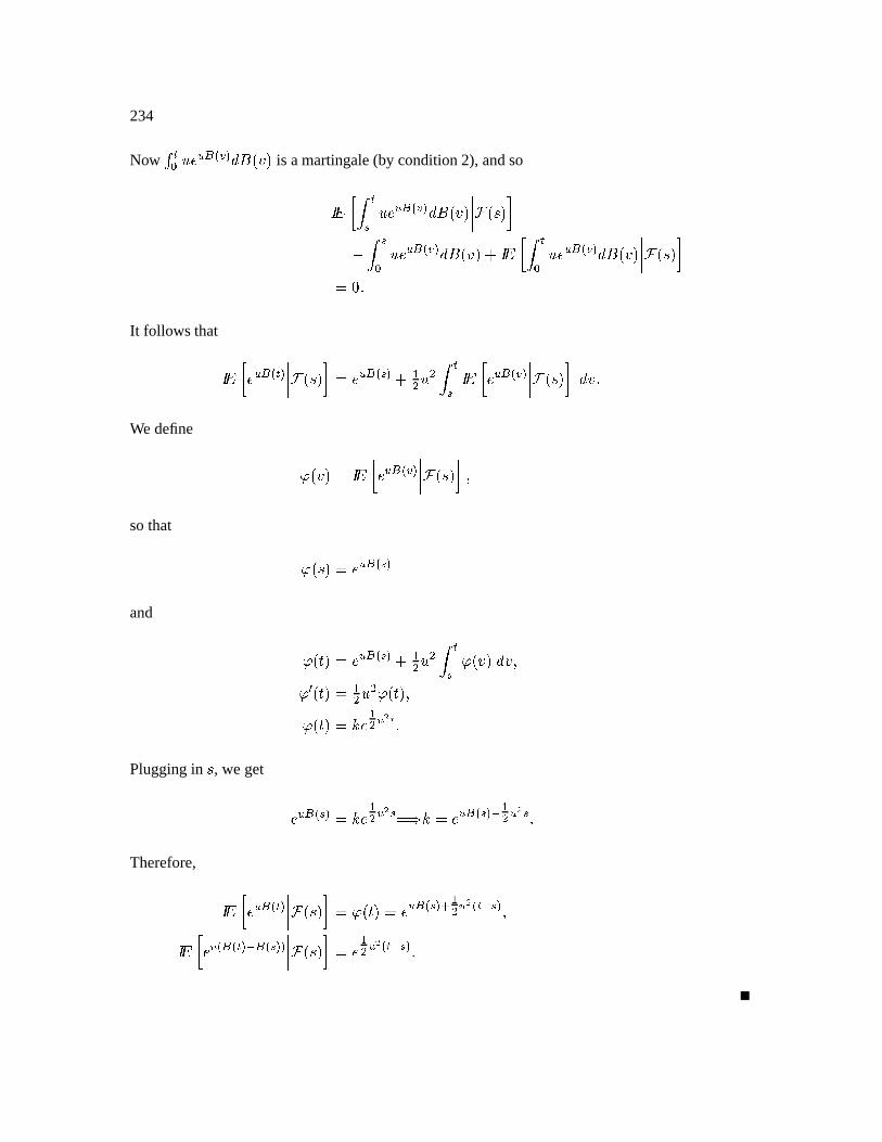
234
Now Z à/ Ä # æ$ë - &0+ ¬ «± is amartingale(by condition2), andsoÞ ß . àê Ä # æÂë - &0+ ¬ «± ¬ é ±"²qµ . ê/ ÄE# æÂë - &,+ ¬ «± Î Þ ß . à/ ÄE# æÂë - &,+ ¬«/± ¬ é ±"²3 ÖIt followsthat Þ ßBĨ# æ-à - ¬ é ± ²3Ĩ# æ¯ê - Î óô ô . àê Þ ß=Ĩ# æ$ë - ¬ é ± & « ÖWe define ì ¬«/±d²3Þ ßBÄE# æ$ë - ¬ é ±°®sothat ì ¬ é ±d²3Ĩ# æ¯ê -and ì ¬B×±²3Ĩ# æ¯ê - Î óô ô . àê ì ¬ «± & «|®ì®í ¬B×±² óô ô ì ¬B×˱h®ì ¬B×±²?îeÄ óô # [ à ÖPluggingin é , we get Ä # æ²ê - ²?îeÄ óô # [ ê ² îx²TÄ # æ²ê - Å óô # [ ê ÖTherefore, Þ ß Ä¨# æ-à - ¬ é ± ²
ì ¬ ×˱d²3Ä # æ¯ê - ç óô # [ æ4à Åê - ®Þ ß Ä¨#æ æ-à - Å æ²ê -- ¬ é ± ²3Ä óô # [ æ4àÅÍê - Ö
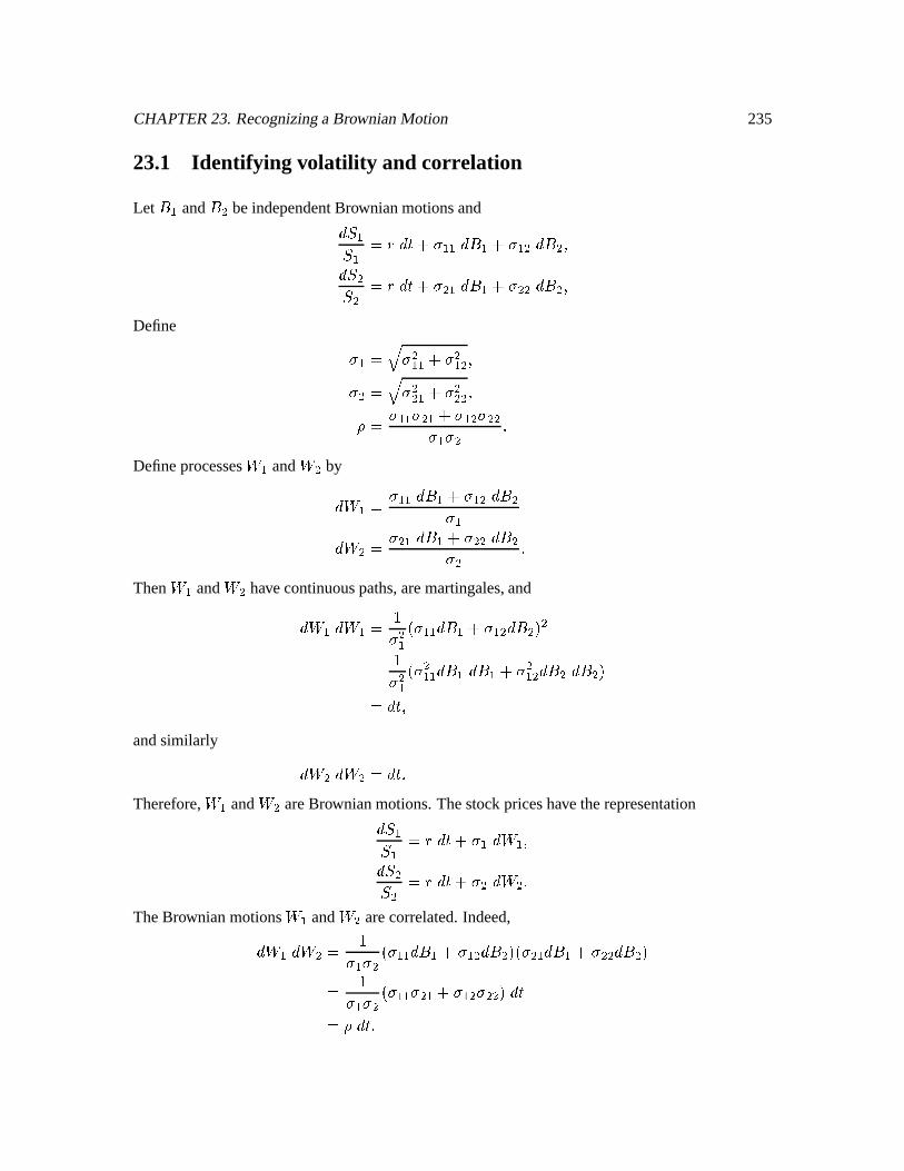
CHAPTER23. Recognizinga BrownianMotion 235
23.1 Identifying volatility and correlation
Let+ ó and
+ ô beindependentBrownianmotionsand& ¯ ó¯ ó ² ¾ & × Î À óJó &,+ ó Î À ó ô &0+ ô ®& ¯ ô¯ ô ² ¾ & × Î À ô ó &,+ ó Î À ôJô &0+ ô ®Define À ó ²ðï À ô óJó Î À ô ó ô ®À ô ² ï À ôô ó Î À ôôJô ®x² À óJó À ô ó Î À ó ô À ôJôÀ ó À ô ÖDefineprocessesñ ó and ñ ô by& ñ ó ² À óJó &,+ ó Î À ó ô &0+ ôÀ ó& ñ ô ² À ô ó &,+ ó Î À ôJô &0+ ôÀ ô ÖThen ñ ó and ñ ô havecontinuouspaths,aremartingales,and& ñ ó & ñ ó ² ´À ô ó ¬ À óJó &,+ ó Î À ó ô &0+ ô ± ô² ´À ô ó ¬ À ô óJó &,+ ó &,+ ó Î À ô ó ô &0+ ô &,+ ô ±² & ×\®andsimilarly & ñ ô & ñ ô ² & × ÖTherefore,ñ ó and ñ ô areBrownianmotions.Thestockpriceshave therepresentation& ¯ ó¯ ó ² ¾ & × Î À ó & ñ ó ®& ¯ ô¯ ô ² ¾ & × Î À ô & ñ ô ÖTheBrownianmotionsñ ó and ñ ô arecorrelated.Indeed,& ñ ó & ñ ô ² ´À ó À ô ¬ À óJó &,+ ó Î À ó ô &,+ ô ±ü¬À ô ó &,+ ó Î À ôJô &,+ ô ±² ´À ó À ô ¬ À óJó À ô ó Î À ó ô À ôJô ± & ײò & × Ö
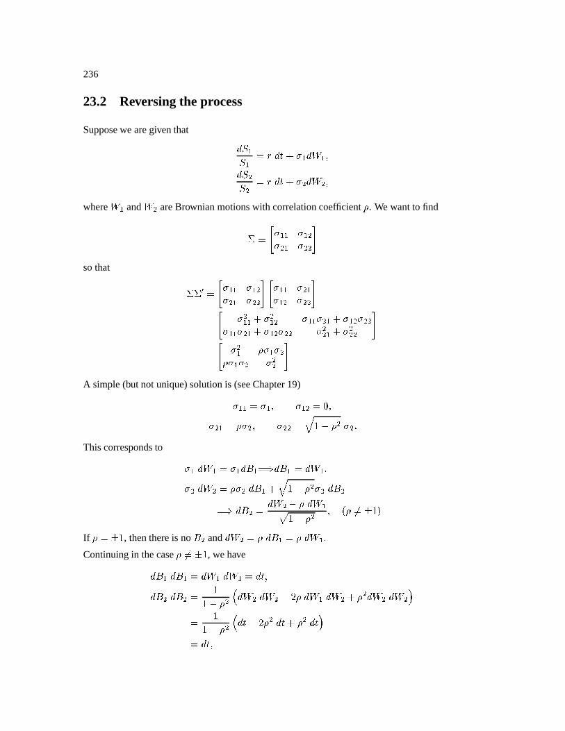
236
23.2 Reversing the process
Supposewe aregiventhat & ¯ ó¯ ó ² ¾ & × Î À ó & ñ ó ®& ¯ ô¯ ô ² ¾ & × Î À ô & ñ ô ®whereñ ó and ñ ô areBrownianmotionswith correlationcoefficient . We wantto findó ² ³ À óJó À ó ôÀ ô ó À ôJô Ãsothat ónó í ² ³ À óJó À ó ôÀ ô ó À ôJô à ³ À óJó À ô óÀ ó ô À ôô ò¹³ À ô óJó Î À ô ó ô À óJó À ô ó Î À ó ô À ôJôÀ óJó À ô ó Î À ó ô À ôJô À ôô ó Î À ôôJô ò¹³ À ô ó bÀ ó À ôbÀ ó À ô À ôô ÃA simple(but not unique)solutionis (seeChapter19)À óó ²KÀ ó ® À ó ô ²3e®À ô ó ²~eÀ ô ® À ôô ² ï ´£µ ô À ô ÖThiscorrespondsto À ó & ñ ó ²3À ó &,+ ó ² &,+ ó ² & ñ ó ®À ô & ñ ô ²~eÀ ô &,+ ó Î ï ´ÌµÉ ô À ô &,+ ô² &,+ ô ² & ñ ô µÉ & ñ óô ´£µÉ ô ® ¬õ²?tE´ü±If ²?tE´ , thenthereis no
+ ô and& ñ ô ²~ &,+ ó ²~ & ñ ó Ö
Continuingin thecaseõ²?tE´ , wehave&,+ ó &,+ ó ² & ñ ó & ñ ó ² & ×\®&,+ ô &,+ ô ² ´´£µÉ ô ' & ñ ô & ñ ô µ Á & ñ ó & ñ ô Î ô & ñ ô & ñ ô )² ´´£µÉ ô ' & ×ɵ Á ô & × Î ô & × )² & ×®
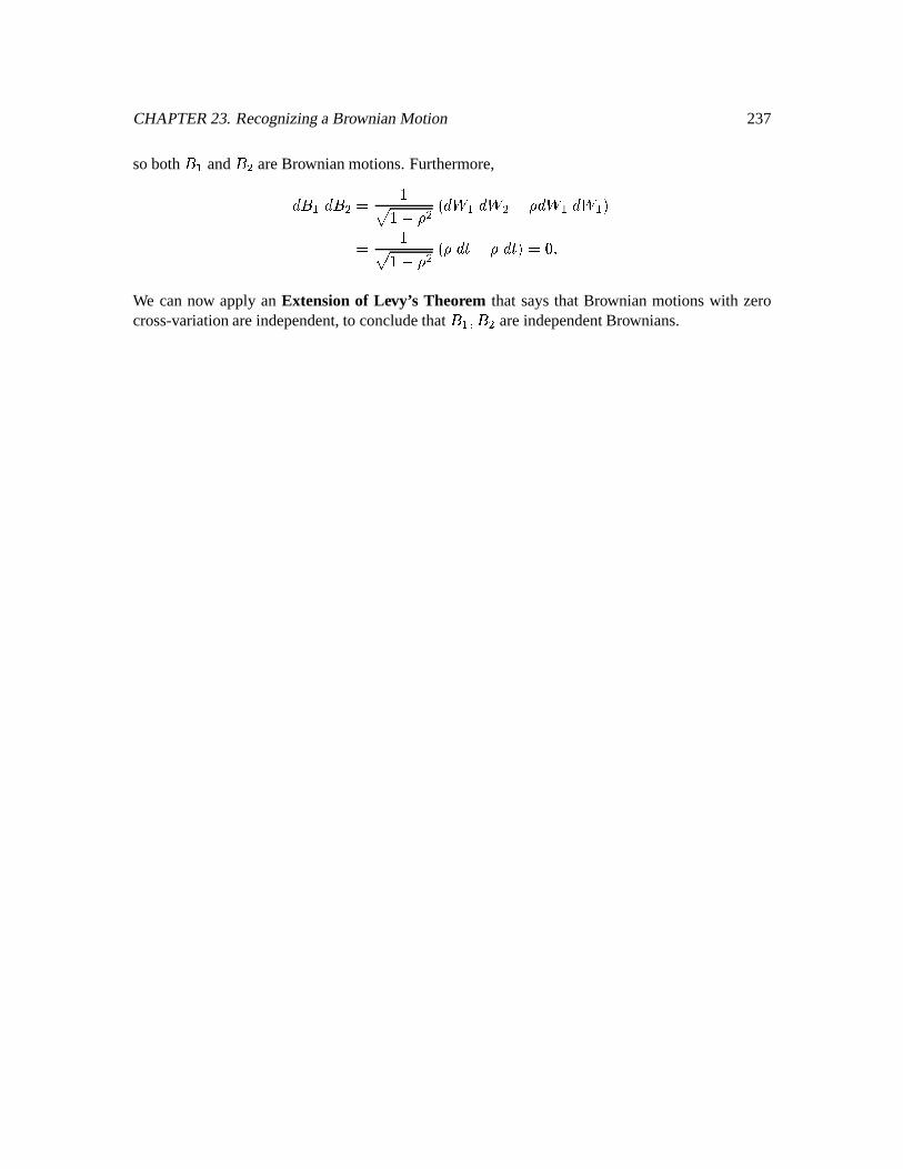
CHAPTER23. Recognizinga BrownianMotion 237
soboth+ ó and
+ ô areBrownianmotions.Furthermore,&0+ ó &,+ ô ² ´ô ´£µÇ ô ¬ & ñ ó & ñ ô µÉ & ñ ó & ñ ó ±² ´ô ´£µÇ ô ¬¯ & ×òµÇ & ×±d²3 ÖWe cannow apply an Extension of Levy’s Theorem that saysthat Brownian motionswith zerocross-variationareindependent,to concludethat
+ ó ® + ô areindependentBrownians.

238
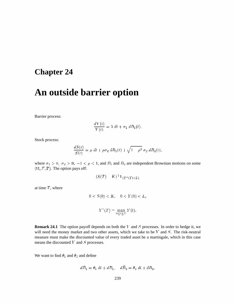
Chapter 24
An outsidebarrier option
Barrierprocess: & @ ¬B×˱@ ¬B×˱ ²÷ö & × Î À ó &0+ ó ¬B×˱ ÖStockprocess: & ¯°¬ ×˱¯Õ¬B×˱ ²~ø & × Î eÀ ô &,+ ó ¬B×˱ Î ï ´£µÉ ô À ô &0+ ô ¬B×±h®where À ó ö e®QÀ ô öTe®£µ´EÜ >Ü¿´ , and
+ ó and+ ô areindependentBrownianmotionsonsome¬ ® ®µ± . Theoptionpaysoff: ¬ ¯°¬ ½ ±òµÍÈ ± ç è é*ùdë æ4Ç - ìeíeî
at time½
, where xÜ"¯°¬ 2±©ÜÈÔ® EÜ @ ¬  § ®@ 2¬ ½ ±d²øaú D/Eû à û Ç @ ¬B×± ÖRemark 24.1 Theoptionpayoff dependson boththe @ and ¯ processes.In orderto hedgeit, wewill needthemoney marketandtwo otherassets,which we taketo be @ and ¯ . Therisk-neutralmeasuremustmakethediscountedvalueof every tradedassetbea martingale,which in this casemeansthediscounted@ and ¯ processes.
We wantto find ü ó and ü ô anddefine& + ó ² ü ó & × Î &,+ ó ® & + ô ² ü ô & × Î &0+ ô ®239
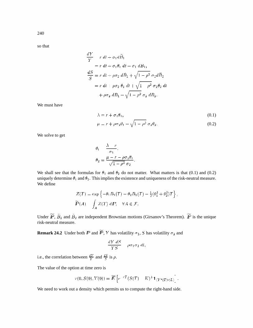
240
sothat & @@ ² ¾ & × Î À ó & + ó² ¾ & × Î À ó ü ó & × Î À ó &,+ ó ®& ¯¯ ² ¾ & × Î bÀ ô & + ó Î ï ´£µ ô À ô & + ô² ¾ & × Î bÀ ô ü ó & × Î ï ´ÌµÉ ô À ô ü ô & ×Î bÀ ô &,+ ó Î ï ´Qµ ô À ô &,+ ô ÖWe musthave öx² ¾QÎ À ó ü ó ® (0.1)øݲ ¾QÎ bÀ ô ü ó Î ï ´ÌµÇ ô À ô ü ô Ö (0.2)
We solveto get ü ó ² öxµ ¾À ó ®ü ô ² øݵ ¾ µÉeÀ ô ü óô ´ÌµÉ ô À ô ÖWe shall seethat the formulasfor ü ó and ü ô do not matter. What mattersis that (0.1) and(0.2)uniquelydetermineü ó and ü ô . Thisimpliestheexistenceanduniquenessof therisk-neutralmeasure.We define ý ¬ ½ ±d² BEDF G µ ü ó + ó ¬ ½ ±dµ ü ô + ô ¬ ½ ±òµ óô ¬ ü ô ó Î ü ôô ± ½ I ®y Þ z ¬PþÕ±d² .½ÿ ý ¬ ½ ± & Þ zQ® dþ ÖUnder y Þ z ,
+ ó and+ ô areindependentBrownianmotions(Girsanov’s Theorem). y Þ z is theunique
risk-neutralmeasure.
Remark 24.2 Underboth Þ z and y Þ z , @ hasvolatility À ó , ¯ hasvolatility À ô and& @ & ¯@ ¯ ²~eÀ ó À ô & ×®i.e., thecorrelationbetween
ùù and êê is .
Thevalueof theoptionat timezerois«¬e®\¯Õ¬ 2±h® @ ¬ 2±J±ò² yÞ ß ä Ä ÅeÆÇ ¬ ¯Õ¬ ½ ±0µ·ÈÔ± ç è é*ùdë æ4Ç - ìeíeî ï ÖWe needto work outa densitywhichpermitsusto computetheright-handside.
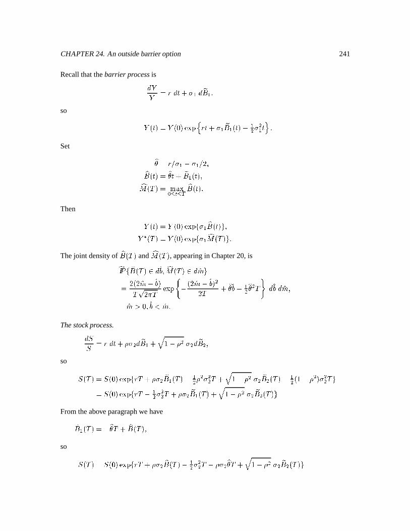
CHAPTER24. An outsidebarrieroption 241
Recallthatthebarrier processis& @@ ² ¾ & × Î À ó & + ó ®so @ ¬ ×˱d² @ ¬ 2± BEDFCG ¾ × Î À ó + ó ¬B×±dµ óô À ô ó ×4I ÖSet ü ² ¾ ^2À ó µ·À ó ^ Á ®+ ¬ ×˱d² ü × Î + ó ¬B×˱i® ¬ ½ ±d²øaú D/Eû à û Ç + ¬B×± ÖThen @ ¬ ×˱d² @ ¬ 2± BEDF ûCÀ ó + ¬B×˱ ÿ ®@ ¬ ½ ±d² @ ¬ 2± BEDF ûCÀ ó ¬ ½ ± ÿ ÖThejoint densityof
+ ¬ ½ ± and ¬ ½ ± , appearingin Chapter20, isy Þ zEû + ¬ ½ ± &» ® ¬ ½ ± & ÿ² Á ¬ Á ñµ » ±½ ¼ Á ½ BED!F 9 µ ¬ Á @µ » ± ôÁ ½ Î ü » µ óô ü ô ½ Ô &»£& Ô® öe® » Ü Ö
Thestock process.& ¯¯ ² ¾ & × Î eÀ ô & + ó Î ï ´ÌµÉ ô À ô & + ô ®so ¯Õ¬ ½ ±ò²3¯°¬2± BED!F û ¾ ½ Î bÀ ô + ó ¬ ½ ±òµ óô ô À ôô ½ Î ï ´ÌµÉ ô À ô + ô ¬ ½ ±dµ óô ¬´Qµ ô ±JÀ ôô ½ ÿ²3¯°¬2± BED!F û ¾ ½ µ óô À ôô ½ Î bÀ ô + ó ¬ ½ ± Î ï ´QµÇ ô À ô + ô ¬ ½ ± ÿFromtheaboveparagraphwe have+ ó ¬ ½ ±ò²qµ ü ½ Î + ¬ ½ ±h®so ¯Õ¬ ½ ±ò²3¯°¬2± BED!F û ¾ ½ Î bÀ ô + ¬ ½ ±òµ óô À ôô ½ µbÀ ô ü ½ Î ï ´£µÉ ô À ô + ô ¬ ½ ± ÿ
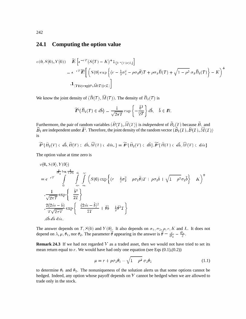
242
24.1 Computing the option value«+¬ e®\¯Õ¬ 2±h® @ ¬ 2±±É² y Þ ß ä Ä ÅbÆÇ ¬¯°¬ ½ ±0µ·ÈÔ± ç èbé*ùë æ4Ç - ìeíeî ï²3Ä ÅeÆËÇ y Þ ß Q ¯°¬ 2± BEDF Ú ¬ ¾ µ óô À ôô µÉeÀ ô ü ± ½ Î eÀ ô + ¬ ½ ± Î ï ´ÌµÉ ô À ô + ô ¬ ½ ± Û µÍÈ R çÖ è é*ù æ / - À k æ4Ç - ìeíeî We know thejoint densityof ¬ + ¬ ½ ±i® ¬ ½ ±J± . Thedensityof
+ ô ¬ ½ ± isy Þ zEû + ô ¬ ½ ± & º» ÿ ² ´¼ Á ½ BEDF 9Yµ º» ôÁ ½ Ô & º» ® º» Þ M ÖFurthermore,thepairof randomvariables¬ + ¬ ½ ±h® ¬ ½ ±J± is independentof
+ ô ¬ ½ ± because+ ó and+ ô areindependentundery Þ z . Therefore,thejoint densityof therandomvector ¬ + ô ¬ ½ ±h® + ¬ ½ ±h® ¬ ½ ±J±
isy Þ z û + ô ¬ ½ ± & º» ® + ¬ ½ ± & » ® ¬ ½ ± & Ô® ÿ ² y Þ záû + ô ¬ ½ ± & º» ÿ Ö y Þ z û + ¬ ½ ± & » ® ¬ ½ ± & ÿTheoptionvalueat time zerois«+¬ e®¯°¬ Ó±h® @ ¬2±J±²3ÄÅeÆÇ kÀ k . / !.Å#" ".Å#" Q2¯°¬ Ó± BED!F Ú ¬ ¾ µ óô À ôô µÉbÀ ô ü ± ½ Î bÀ ô » Î ï ´£µÉ ô À ô º» Û µÍÈ R çÖ ´¼ Á ½ BED!F 9 µº» ôÁ ½ ÔÖ Á ¬ Á ñµ » ±½ ¼ Á ½ BED!F 9 µ ¬ Á µ » ± ôÁ ½ Î ü » µ óô ü ô ½ ÔÖ & º»O&»l& ÖThe answerdependson
½ ®\¯Õ¬ 2± and @ ¬2± . It alsodependson À ó ®\À ô ®+® ¾ ®JÈ and § . It doesnotdependon ö®µød® ü ó ® nor ü ô . Theparameter
ü appearingin theansweris
ü ² ÆÀ k µ À kô ÖRemark 24.3 If we hadnot regarded@ asa tradedasset,thenwe would not have tried to setitsmeanreturnequalto ¾ . We wouldhavehadonly oneequation(seeEqs(0.1),(0.2))øݲ ¾Î bÀ ô ü ó Î ï ´ÌµÉ ô À ô ü ô (1.1)
to determineü ó and ü ô . The nonuniquenessof the solutionalertsus thatsomeoptionscannotbehedged.Indeed,any optionwhosepayoff dependson @ cannotbehedgedwhenwe areallowedtotradeonly in thestock.
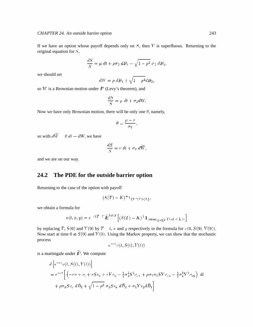
CHAPTER24. An outsidebarrieroption 243
If we have an option whosepayoff dependsonly on ¯ , then @ is superfluous.Returningto theoriginalequationfor ¯ , & ¯¯ ²~ø & × Î bÀ ô &0+ ó Î ï ´£µÉ ô À ô &,+ ô ®weshouldset & ñ ²~ &,+ ó Î ï ´ÌµÇ ô &,+ ô ®so ñ is a BrownianmotionunderÞ z (Levy’s theorem),and& ¯¯ ²~ø & × Î À ô & ñ ÖNow wehave only Brownianmotion,therewill beonly one ü , namely,ü ² ø>µ ¾À ô ®sowith
& yñ ² ü & × Î & ñ ® wehave & ¯¯ ² ¾ & × Î À ô & yñ ®andweareonourway.
24.2 The PDE for the outsidebarrier option
Returningto thecaseof theoptionwith payoff¬¯°¬ ½ ±òµÍÈÔ±Jçèbé*ù ë æ4Ç - ìeíeî ®weobtaina formulafor«+¬B×® Ø ®4A/±ò²3ÄÅbÆæ-Ç1Åeà - yÞ ß à â ãâ K ä ¬ ¯Õ¬ ½ ±òµÍÈÔ±Jçè é%$'& (*)+,).- ù æ$# - ìíeî ® ïby replacing
½, ¯°¬2± and @ ¬ 2± by
½ µÔ× , Ø and A respectively in theformulafor «+¬ e®¯°¬ 2±i® @ ¬ Ó±J± .Now startat time0 at ¯°¬ Ó± and @ ¬ 2± . UsingtheMarkov property, we canshow thatthestochasticprocess ÄÅeÆà «¬ ×\®\¯Õ¬B×˱i® @ ¬B×˱J±is amartingaleundery Þ z . We compute& ä Ä ÅeÆà «¬ ×\®\¯Õ¬B×˱i® @ ¬B×˱J± ï²3ÄÅeÆà0 ' µ ¾ « Î « à Îj¾ ¯« ã Î"¾ @ « K Î óô À ôô ¯ ô « ãhã Î eÀ ó À ô ¯ @ « ãEK Î óô À ô ó @ ô « KK ) & ×Î bÀ ô ¯©« ã & + ó Î ï ´£µÉ ô À ô ¯©« ã & + ô Î À ó @ « K & + ó
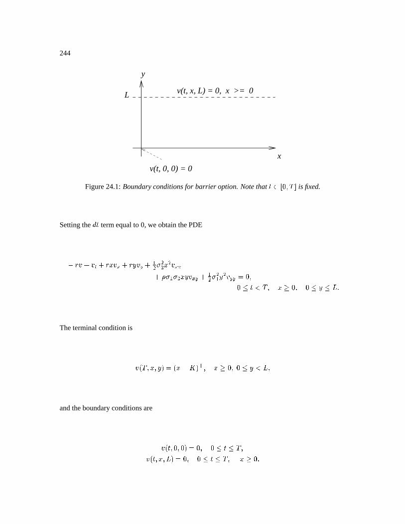
244
L
v(t, 0, 0) = 0
x
y
v(t, x, L) = 0, x >= 0
Figure24.1:Boundaryconditionsfor barrier option.Notethat × Ç ® ½£ is fixed.
Settingthe& × termequalto 0, we obtainthePDE
µ ¾ « Î « à Îj¾ Ø « ã ξ A« K Î óô À ôô Ø ô « ãhãÎ eÀ ó À ô Ø A/« ãEK Î@óô À ô ó A ô « KK ²3e® Ù × Ü ½ ® Ø ý"e® Ù A Ù§ ÖTheterminalconditionis
«+¬ ½ ® Ø ®4A/±+²ñ¬ Ø µ·ÈÔ± ç ® Ø ýe®d Ù A~Ü § ®andtheboundaryconditionsare
«¬B×®\e®2±1²3® Ù × Ù ½ ®«¬B×® Ø ® § ±0²3e® Ù × Ù ½ ® Ø ý Ö
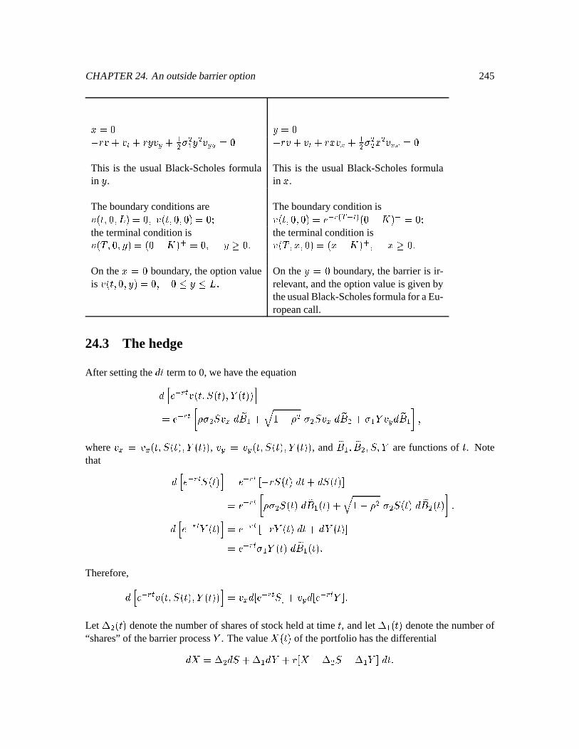
CHAPTER24. An outsidebarrieroption 245
Ø ² A²Kµ ¾ « Î « à Î"¾ A« K Î óô À ô ó A ô « KK ²3 µ ¾ « Î « à Îj¾ Ø « ã Î óô À ôô Ø ô « ãhã ²3This is the usualBlack-Scholesformulain A . This is the usualBlack-Scholesformula
in Ø .Theboundaryconditionsare Theboundaryconditionis«+¬B×\®e® § ±1²3e®«+¬B×®\e®2±+²3eþ «+¬B×\®e®\2±0²3Ä ÅeÆæ4Ç0Åeà - ¬ µÍÈÔ± ç ²3eþtheterminalconditionis theterminalconditionis«+¬ ½ ®e®JA±+²ñ¬ Õµ·ÈÔ± ç ²3e® Axý Ö «+¬ ½ ® Ø ®\Ó±²@¬ Ø µÍÈÔ± ç ® Ø ý ÖOn the Ø ²q boundary, theoptionvalueis «¬ ×\®\®JA±1²3e® Ù A Ù§ Ö On the A>² boundary, thebarrieris ir-
relevant,andtheoptionvalueis givenbytheusualBlack-Scholesformulafor aEu-ropeancall.
24.3 The hedge
After settingthe& × termto 0, wehave theequation& ä-Ä ÅeÆà «+¬B×\®¯°¬B×±h® @ ¬B×˱± ï²3Ä ÅeÆà eÀ ô ¯« ã & + ó Î ï ´£µÇ ô À ô ¯« ã & + ô Î À ó @ « K & + ó ®
where « ã ² « ã ¬B×\®¯°¬B×±h® @ ¬B×±J± , « K ² « K ¬B×®\¯°¬ ×˱h® @ ¬B×±J± , and+ ó ® + ô ®¯d® @ arefunctionsof × . Note
that & ä Ä ÅeÆËà ¯Õ¬B×˱ ï ²KÄ ÅeÆà µ ¾ ¯Õ¬B×˱ & × Î & ¯Õ¬B×˱ ²KÄÅeÆà bÀ ô ¯°¬B×± & + ó ¬B×˱ Î ï ´ÌµÉ ô À ô ¯°¬B×± & + ô ¬B×± Ö& ä Ä ÅeÆà @ ¬B×˱ ï ²KÄ ÅeÆà µ ¾ @ ¬B×± & × Î & @ ¬ ×˱ ²KÄ ÅeÆà À ó @ ¬B×± & + ó ¬B×± ÖTherefore,& ä Ä ÅeÆà «¬ ×\®\¯Õ¬B×˱i® @ ¬B×˱J± ï ²K« ã & Ä ÅeÆà ¯ Î « K & Ä ÅbÆà @ ÖLet 8 ô ¬ ×˱ denotethenumberof sharesof stockheldat time × , andlet 8 ó ¬B×± denotethenumberof“shares”of thebarrierprocess@ . Thevalue 7 ¬ ×˱ of theportfolio hasthedifferential& 7 ² 8 ô & ¯ Î 8 ó & @ ξ ´7 µ 8 ô ¯Ôµ 8 ó @ & × Ö
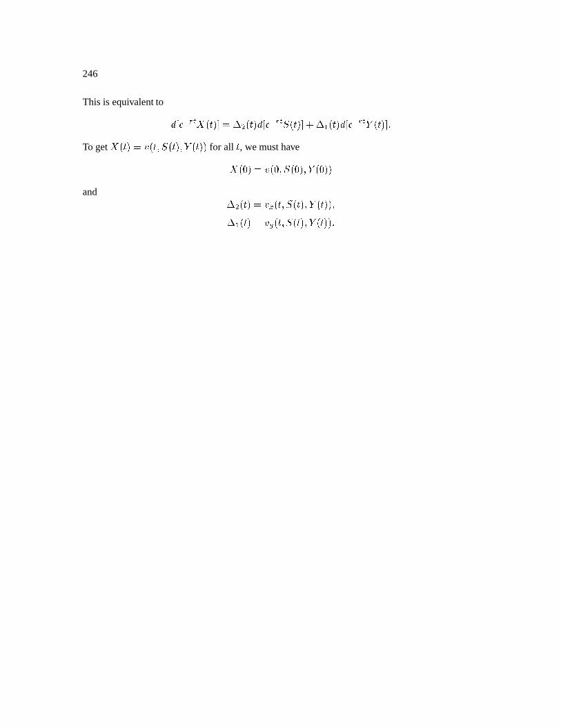
246
This is equivalentto & ÄÅbÆà 7 ¬B×˱ ² 8 ô ¬ ×˱ & ÄÅeÆà ¯°¬B×± Î 8 ó ¬B×˱ & ÄÅeÆËà @ ¬B×˱ ÖTo get 7 ¬B×˱d²K«¬B×®\¯Õ¬B×˱h® @ ¬ ×˱J± for all × , wemusthave7 ¬ 2±ò²3«¬e®\¯Õ¬ 2±h® @ ¬ 2±J±and 8 ô ¬B×±d²3« ã ¬B×\®¯°¬B×±h® @ ¬B×±J±h®8 ó ¬B×˱d²3« K ¬B×\®¯°¬B×±h® @ ¬B×˱± Ö
Chapter 25
American Options
This andthe following chaptersform part of the courseStochasticDifferential Equationsfor Fi-nanceII.
25.1 Preview of perpetual American put& ¯ ² ¾ ¯ & × Î À1¯ &,+Intrinsicvalueat time ×0/|¬ È µÍ¯°¬B×±J± ç ÖLet §<Ç ®\È begiven.Supposeweexercisethefirst time thestockpriceis § or lower. We define÷ í ²3øEùåúûü× ý"eþ\¯Õ¬B×˱ Ù§Qÿ ®« í ¬ Ø ±d²3Þ ßEÄÅbÆ%1 ¬ È µÍ¯°¬ ÷ í ±J±Jç² 9 È µ Ø if Ø>Ù§ ,¬ È8µ § ±JÞ ß Ä ÅeÆ21 if Ø ö § ÖTheplanis to comute« í ¬ Ø ± andthenmaximizeover § to find theoptimalexerciseprice.We needto know thedistributionof ÷ í .25.2 First passagetimes for Brownian motion: first method
(Basedonthereflectionprinciple)
Let+
bea BrownianmotionunderÞ z , let Ø ö begiven,anddefine÷E²3øEùåúûü× ý"eþ + ¬B×˱d² Øÿ Ö÷ is calledthefirst passagetimeto Ø . We computethedistributionof ÷ .247
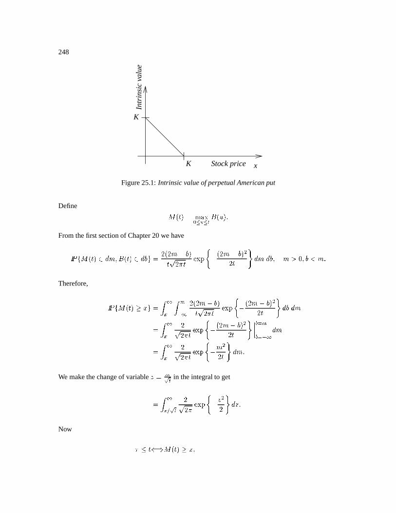
248
K
K
x
Intr
insi
c va
lue
Stock price
Figure25.1: Intrinsic valueof perpetualAmericanput
Define ¬ ×˱²Êø(ú D/Eû # û à + ¬ ± ÖFromthefirst sectionof Chapter20we haveÞ záû ¬B×˱ & Ô® + ¬B×± &» ÿ ² Á ¬ Á @µ » ±× ¼ Á × BED!F 9 µ ¬ Á µ » ± ôÁ × Ô & &» ® öe® » Ü3 ÖTherefore, Þ záû ¬B×˱Ìý Ø+ÿ ² . "ã . !Å#" Á ¬ Á @µ » ±× ¼ Á × BEDF 9Qµ ¬ Á µ » ± ôÁ × Ô &»£& ² . "ã Á¼ Á × BED!F 9 µ ¬ Á ñµ » ± ôÁ × Ô 4 w !4 w Å#" & ² . "ã Á¼ Á × BED!F 9 µ ôÁ × Ô & ÖWe makethechangeof variable5 ² !6 à in theintegral to get² . "ã87 6 à Á¼ Á BED!F 9Qµ 5 ôÁ Ô & 5 ÖNow ÷ Ù × T ¬B×±£ý Ø ®
CHAPTER25. AmericanOptions 249
so Þ záûC÷ & × ÿ ² 99 × Þ záûC÷ Ù × ÿ & ײ 99 × Þ zaû ¬B×±Qý Ø+ÿ & ײ¹³ 99 ×L. "ã87 6 à Á¼ Á BED!F 9 µ 5 ôÁ Ô & 5 à & ײqµ Á¼ Á BED!F 9Qµ Ø ôÁ × Ô Ö 99 × Q ؼ × R & ײ Ø× ¼ Á × BED!F 9 µ Ø ôÁ × Ô & × ÖWe alsohave theLaplacetransformformulaÞ ßEÄ Å#:;1 ² . "/ Ä Å<:à Þ záûC÷ & × ÿ²3Ä Åeã 6 ô : ® ; ö Ö (SeeHomework)
Reference:KaratzasandShreve,BrownianMotion andStochasticCalculus,pp95-96.
25.3 Drift adjustment
Reference:Karatzas/Shreve,BrownianmotionandStochasticCalculus, pp196–197.
For Ù × Ü ª , define + ¬B×±d² ü × Î + ¬ ×˱h®ý ¬B×˱©² BED!F û/µ ü + ¬ ×˱©µ óô ü ô × ÿ ®² BED!F û/µ ü + ¬B×˱ Î óô ü ô × ÿ ®Define º÷x²3øEùåú+û × ýþ + ¬B×±² Øÿ ÖWe fix a finite time
½andchangetheprobabilitymeasure“only up to
½”. More specifically, with½
fixed,define y Þ z ¬cþ°±d² . ÿ ý ¬ ½ ± & zQ® þ ¬ ½ ± ÖUnder y Þ z , theprocess+ ¬B×±h®\ Ù × Ù ½ , is a (nondrifted)Brownianmotion,soy Þ zEû º÷ & × ÿ ²KÞ záûC÷ & × ÿ² Ø× ¼ Á × BED!F 9Qµ Ø ôÁ × Ô & ×\® EÜj× Ù ½ Ö
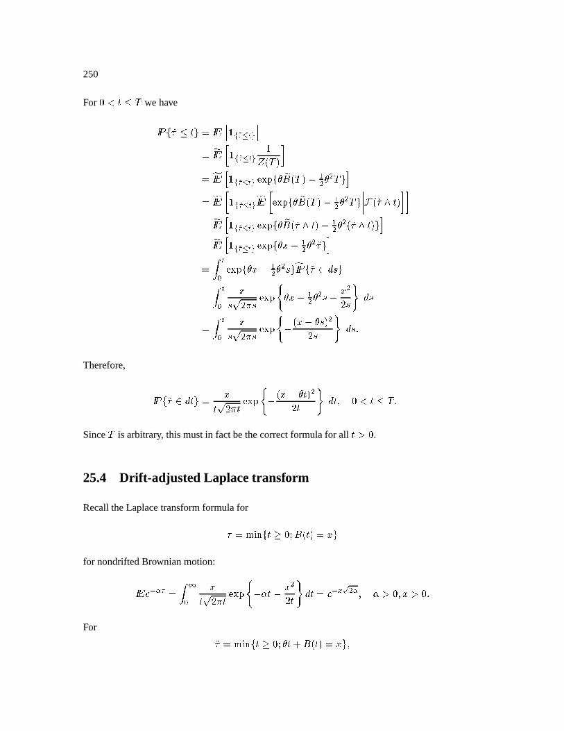
250
For EÜj× Ù ½ we haveÞ záû º÷ Ù × ÿ ²KÞ ß ä èeé>=1 û à î ï² yÞ ß è é>=1 û à î ´ý ¬ ½ ± ² yÞ ß ä è é>=1 û à î BEDF û ü + ¬ ½ ±dµ óô ü ô ½ ÿ ï² yÞ ß è|é>=1 û à î y Þ ß BED!F û ü + ¬ ½ ±dµ óô ü ô ½ ÿ ¬ º÷ >×± ½² yÞ ß ä è é>=1 û à î BEDF û ü + ¬ º÷Ì ×˱dµ óô ü ô ¬ º÷Ì ×˱ ÿ ï² yÞ ß ä èeé>=1 û à î BEDF û üCØ µ óô ü ô º÷ ÿ ï² . à/ BED!F û üØ µ óô ü ô éÿ y Þ záû º÷ & éÿ² . à/ Øé ¼ Á é BEDF 9 üØ µ óô ü ô é µ Ø ôÁ é Ô & é² . à/ Øé ¼ Á é BEDF 9 µ ¬ Ø µ ü½é ± ôÁ é Ô & é ÖTherefore, Þ záû º÷ & × ÿ ² Ø× ¼ Á × BED!F 9 µ ¬ Ø µ ü ×˱ ôÁ × Ô & ×\® EÜj× Ù ½ ÖSince
½is arbitrary, thismustin factbethecorrectformulafor all × ö" .
25.4 Drift-adjusted Laplacetransform
RecalltheLaplacetransformformulafor÷x²3øEùåúûü×Qýeþ + ¬B×±d² Ø+ÿfor nondriftedBrownianmotion:Þ ß ÄÅ#:;1² . "/ Ø× ¼ Á × BEDF 9 µ ; ×µ Ø ôÁ × Ô & ×ɲ3ÄÅbã 6 ô :+® ; ö"e® Ø ö" ÖFor º÷x²3ø ù úûü×Qýeþ ü × Î + ¬B×±² Øÿ ®
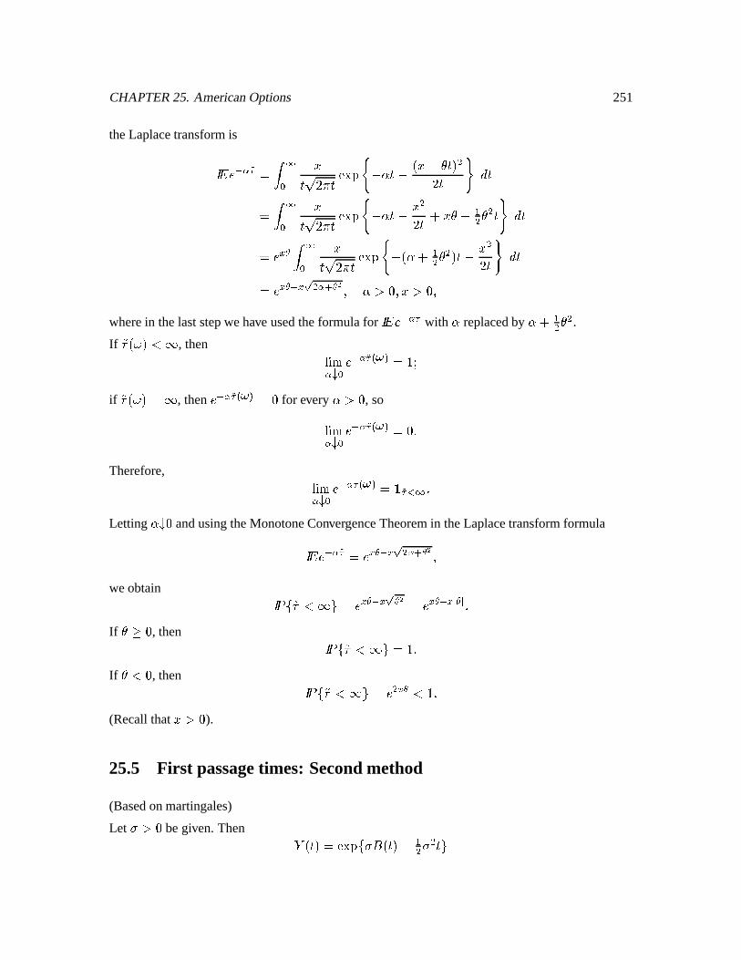
CHAPTER25. AmericanOptions 251
theLaplacetransformisÞ ßEÄ Å#: =1 ² . "/ Ø× ¼ Á × BED!F 9£µ ; ×dµ ¬ Ø µ ü ×± ôÁ × Ô & ײ . "/ Ø× ¼ Á × BED!F 9 µ ; ×dµ Ø ôÁ ×Î Øü µ óô ü ô × Ô & ײ3Ä ã8? . "/ Ø× ¼ Á × BED!F 9 µ¬ ; Î óô ü ô ±×ɵ Ø ôÁ × Ô & ײ3Ä ã8?Åeã 6 ô :2ç@? [ ® ; ö® Ø öe®wherein thelaststepwehave usedtheformulafor Þ ß Ä Å#:;1 with ; replacedby ; Î óô ü ô .If º÷1¬ ±£Ü ª , then Ð ù ø:;A / ÄÅ#: =1æ - ²q´2þif º÷1¬ ±d² ª , then Ä Å<: =1æ - ²K for every ; ö , soÐ ù ø:;A / Ä Å#: =1æ - ²3 ÖTherefore, Ð ùåø:;A / ÄÅ<: =1æ - ² è =1 ì " ÖLetting ; A andusingtheMonotoneConvergenceTheoremin theLaplacetransformformulaÞ ßEÄÅ#: =1²3Äiã8?JÅeã 6 ô :Óç? [ ®weobtain Þ záû º÷õÜ ª"ÿ ²3Ähã8?Åeã 6 ? [ ²3Äiã8?JÅeãB ?,B ÖIf ü ý , then Þ záû º÷>Ü ª"ÿ ²q´ ÖIf ü Ü , then Þ záû º÷õÜ ª"ÿ ²3Ä ô ã8? Ü3´ Ö(Recallthat Ø ö" ).25.5 First passagetimes: Secondmethod
(Basedonmartingales)
Let ÀÔö begiven.Then @ ¬B×±d² BED!F ûCÀ + ¬ ×˱©µ óô À ô × ÿ
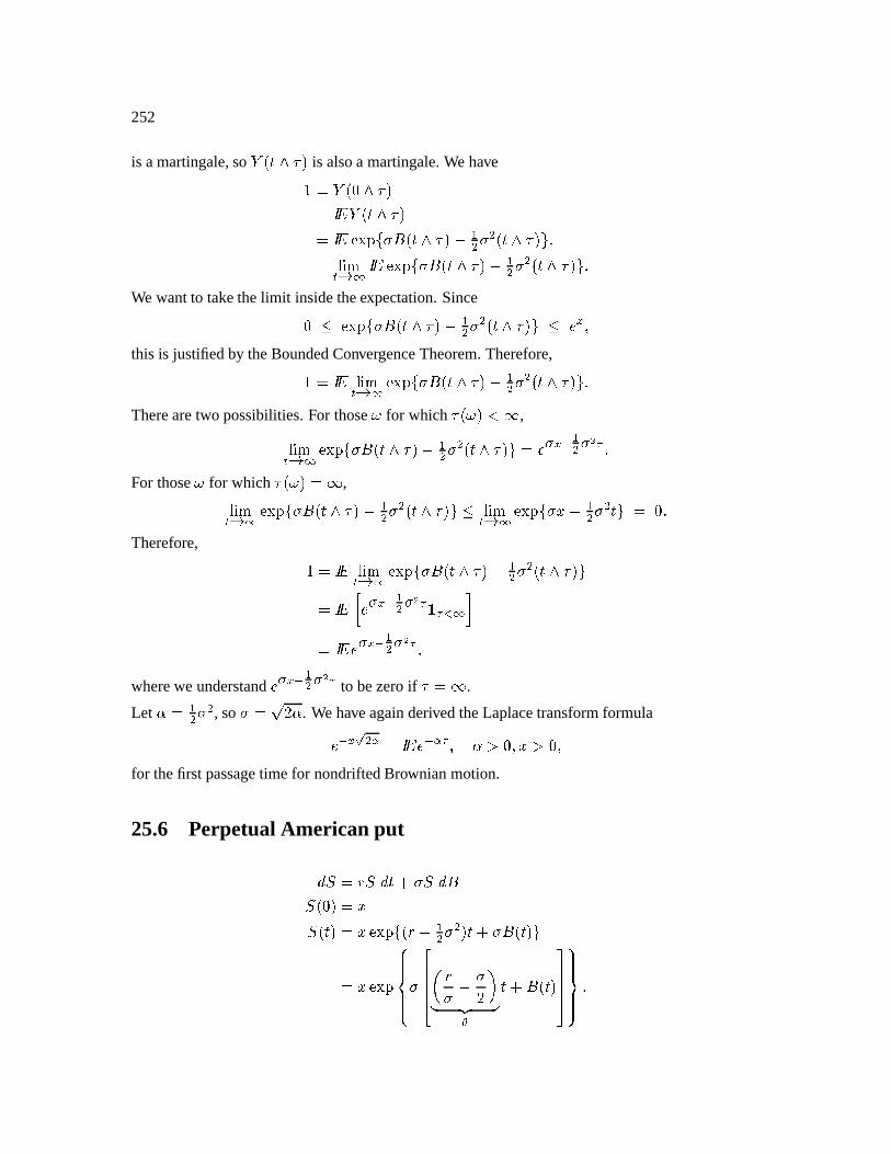
252
is amartingale,so @ ¬B×>÷e± is alsoa martingale.We have´Õ² @ ¬ C>÷e±²3Þ ß @ ¬B×>÷e±²3Þ ß BEDF ûCÀ + ¬B×Ý÷e±dµ óô À ô ¬B×Ý÷e± ÿ Ö² Ð ù øà ¨ " Þ ß BED!F ûCÀ + ¬ × >÷e±µ óô À ô ¬B×õ÷e± ÿ ÖWe wantto takethelimit insidetheexpectation.Since Ù BED!F ûÀ + ¬B×>÷e±dµ óô À ô ¬ ×>÷e± ÿ¿Ù Ähãe®this is justifiedby theBoundedConvergenceTheorem.Therefore,´Õ²3Þ ß Ð ùåøà ¨ " BED!F ûCÀ + ¬ × >÷e±µ óô À ô ¬B×õ÷e± ÿ ÖTherearetwo possibilities.For those for which ÷1¬ ±QÜ ª ,Ð ùåøà ¨ " BEDF ûÀ + ¬B×Ý÷e±dµ óô À ô ¬ ×Ý÷e± ÿ ²3Ä À ãÅ óô À [ 1 ÖFor those for which ÷1¬ ±d² ª ,Ð ùåøà ¨ " BEDF ûCÀ + ¬B×>÷e±dµ óô À ô ¬B×>÷e± ÿÙ Ð ùåøà ¨ " BED!F ûCÀ Ø µ óô À ô × ÿ ² ÖTherefore, ´£²3Þ ß Ð ùåøà ¨ " BED!F ûÀ + ¬B×>÷e±dµ óô À ô ¬B×>÷e± ÿ²3Þ ß Ä À ãÅ óô À [ 1 è 1 ì " ²3Þ ßEÄ À ãÅ óô À [ 1 ®wherewe understandÄ À ãÅ óô À [ 1 to bezeroif ÷ ² ª .
Let ; ² óô À ô , so À>² ¼ Á ; . We haveagainderivedtheLaplacetransformformulaÄÅeã 6 ô :E²3Þ ßEÄÅ#:;1® ; ö"e® Ø ö"e®for thefirst passagetime for nondriftedBrownianmotion.
25.6 Perpetual American put& ¯ ² ¾ ¯ & × Î À+¯ &,+¯Õ¬ 2±ò² د°¬B×±d² ØnBED!F ûb¬ ¾ µ óô À ô ±× Î À + ¬ ×˱ ÿ² ØnBED!F VCCCX CCCY À fhhhi Q ¾À µ À Á R1 243 5? × Î + ¬B×± oqpppr D CCCECCCF Ö
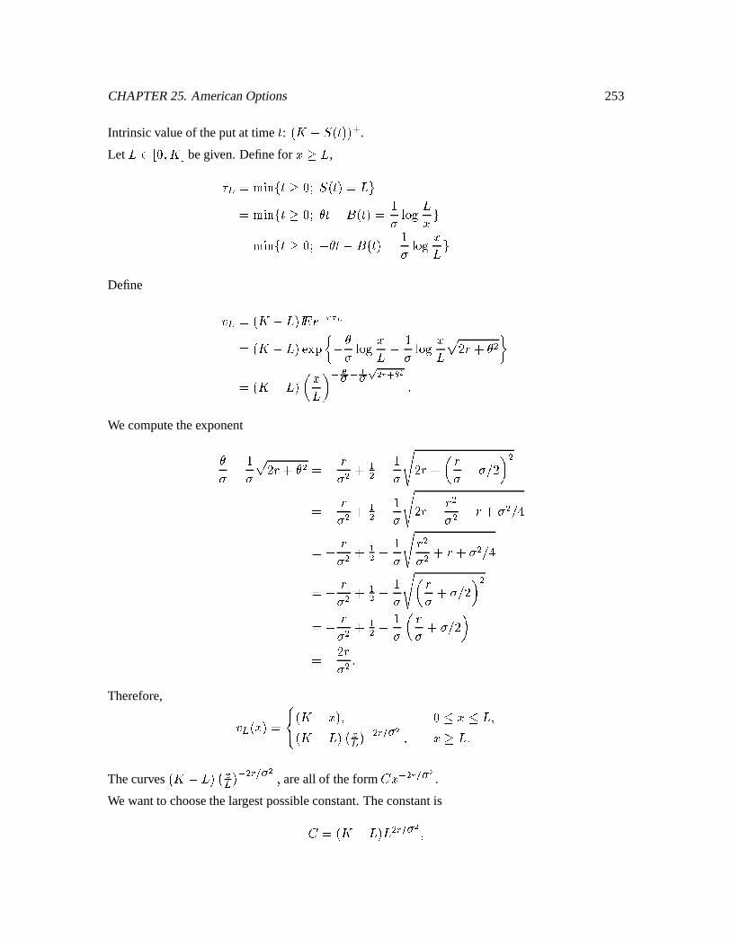
CHAPTER25. AmericanOptions 253
Intrinsicvalueof theputat time × : ¬ È8µa¯°¬B×±J± ç .Let §6É ®\È begiven.Definefor Ø ý § ,÷ í ²3ø ù úû × ýþ¯°¬B×±d² §Qÿ²3ø ù úû × ýþ ü × Î + ¬B×˱©² ´À Ð-Ñ2Ò § Ø ÿ²3ø ù úû × ýþ£µ ü ×ðµ + ¬B×±² ´À Ð-Ñ2Ò Ø§ ÿDefine « í ²ñ¬È8µ § ±JÞ ßEÄ ÅeÆ%1 ²ñ¬È8µ § ± BED!F Ú µ üÀ Ð-Ñ2Ò Ø§ µ ´À Ð-Ñ2Ò Ø§ ô Á ¾QÎ ü ô Û²ñ¬È8µ § ± Q ا R ÅHGÀ Å kÀ 6 ô ÆJç@? [ ÖWe computetheexponentµ üÀ µ ´À ô Á ¾Î ü ô ²Úµ ¾À ô Î óô µ ´ÀJI Á ¾QÎ Q ¾À µ·À^ Á R ô²Úµ ¾À ô Î óô µ ´À I Á ¾QÎ ¾ ôÀ ô µ ¾QÎ À ô ^;K²Úµñ¾À ô Î óô µ ´À I ¾ ôÀ ô Î"¾QÎ À ô ^.K²Úµ ¾À ô Î óô µ ´ÀJI Q¾ÀÔÎ À^ Á R ô²Úµñ¾À ô Î óô µ ´À QQ¾À Î À^ Á R²Úµ Á ¾À ô ÖTherefore, « í ¬ Ø ±d² VX Y ¬ È8µ Ø ±h® ÙØõÙ§ ®¬ È8µ § ±'L ãíNM Å ô Æ7 À [ ® Ø ý § ÖThecurves ¬È µ § ±'L ãíNM Å ô Æ7 À [ ® areall of theform O Ø Å ô ÆP7 À[ .We wantto choosethelargestpossibleconstant.TheconstantisO ²ñ¬ È µ § ± § ô Æ7 ÀÍ[ ®
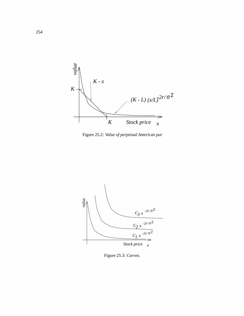
254
σ2-2r/
K
K
xStock price
K - x
(K - L) (x/L)
valu
e
Figure25.2:Valueof perpetualAmericanput
σ 2-2r/C1 x
σ 2-2r/xC2
σ 2-2r/xC3
xStock price
valu
e
Figure25.3:Curves.
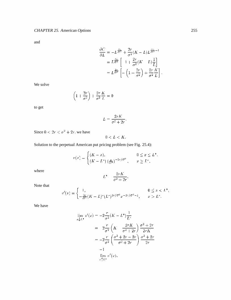
CHAPTER25. AmericanOptions 255
and 9 O9 § ²qµ § [RQÀ [ Î Á ¾À ô ¬ È8µ § ± § [RQÀ [ Å ó² § [RQÀ [ µ´ Î Á ¾À ô ¬ È8µ § ± ´§ ² § [RQÀ [ µ?Qe´ Î Á ¾À ô R Î Á ¾À ô È § ÖWe solve µ Q ´ Î Á ¾À ô R Î Á ¾À ô È § ²3to get § ² Á ¾ ÈÀ ô Î Á ¾ ÖSincexÜ Á ¾ ÜÀ ô Î Á ¾ ® wehave EÜ § ÜÈ ÖSolutionto theperpetualAmericanput pricingproblem(seeFig. 25.4):«+¬ Ø ±d² VX Y ¬ È µ Ø ±h® ÙØ>Ù§ ®¬ È µ § ±'L ãí ë M Å ô ÆP7 À[ ® Ø ý § ®where § £² Á ¾ ÈÀ ô Î Á ¾ ÖNotethat « í ¬ Ø ±d² 9 µ´Ó® ÙØ Ü § ®µ ô ÆÀ [ ¬È µ § ± ¬ § ± ô ÆP7 À[ Ø Å ô Æ7 ÀN[ Å ó ® Ø ö § ÖWe have Ð ùåøãSA í ë «
í ¬ Ø ±d²Úµ Á ¾À ô ¬ È µ § ± ´§ ²Úµ Á ¾À ô Q È µ Á ¾ ÈÀ ô Î Á ¾ R À ô Î Á ¾Á ¾ Ȳڵ Á ¾À ô ¸ À ô Î Á ¾ µ Á ¾À ô Î Á ¾  À ô Î Á ¾Á ¾²Úµ´² Ð ùåøãST í ë «í ¬ Ø ± Ö
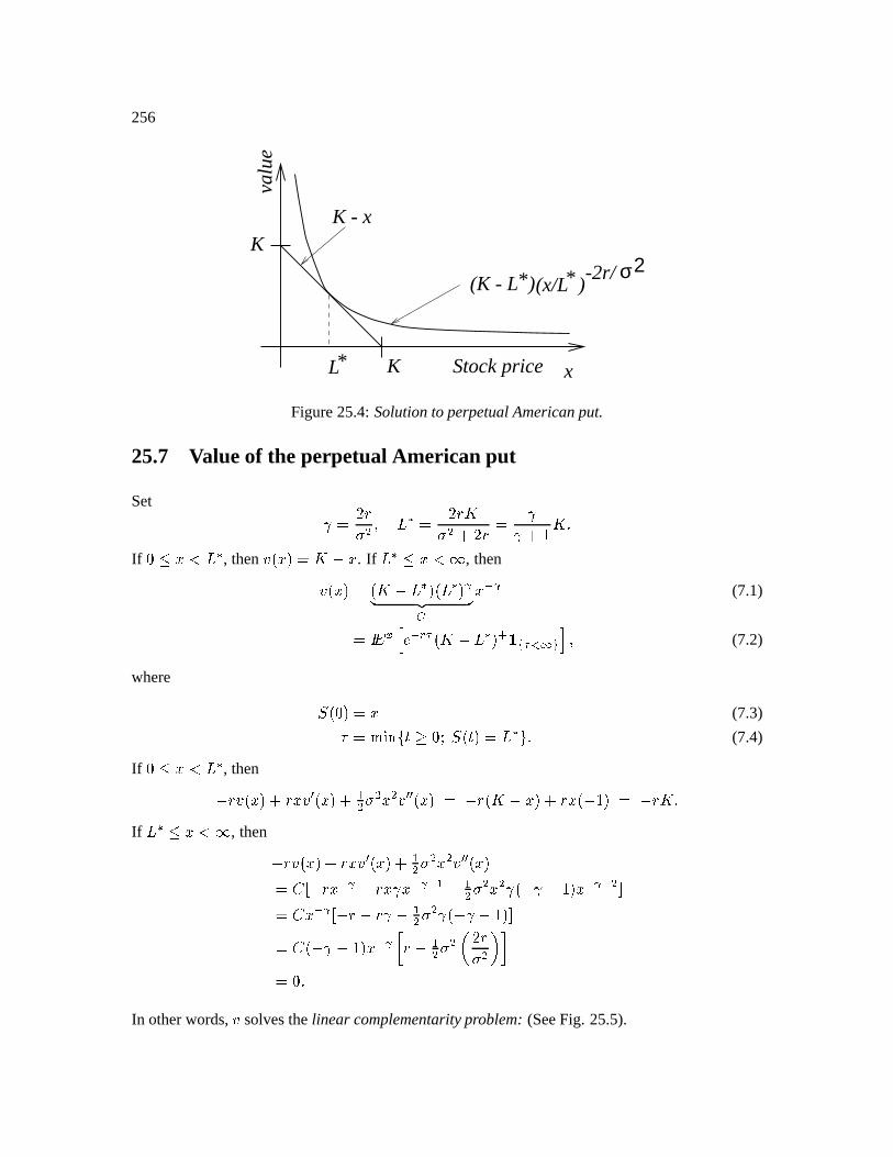
256
σ2-2r/
K
K
xStock price
K - x
valu
e(K - L )(x/L )**
*L
Figure25.4:Solutionto perpetualAmericanput.
25.7 Valueof the perpetual American put
Set UWVYXZ[]\#^ _a` V XZ;b[]\'c XZ V UU ced bgfIf hji3kml _ ` , then n@ok#p V brq k . If _ ` i3kslut , thenn@okp V o bvq _w` p8o _w` pxy z | k@~x (7.1)Ve j ~% o brq _ ` p ;<, ^ (7.2)
where ohp V k (7.3) Ve80 h o p V _ `> f (7.4)
If hji3kml _ ` , thenq Z n@ok#p c Z kn¡ok#p c£¢\ [ \ k \ n¡¡ok#p V q Z o brq k#p c Z kNo q d p V q Z;bgfIf _ ` i3k¤l¥t , then q Z n@okp c Z kn ¡ okp c¦¢\ [ \ k \ n ¡ ¡ ok#pV¨§ª© q Z k@~x q«Z k U k~x~ ¢ q ¢\ [ \ k \ U o q U q d pk~¬x~ \®V¨§ k@~x © q Z¯q«Z U q ¢\ [ \ U o q U q d p V¨§ o q U q d pk ~x±° ZJq ¢\ [ \J² XZ[ \³´V h fIn otherwords, n solvesthe linear complementarityproblem:(SeeFig. 25.5).
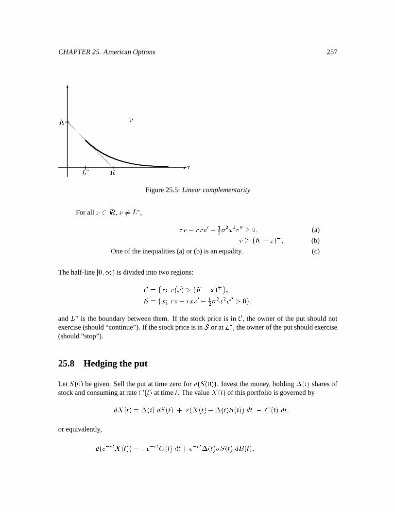
CHAPTER25. AmericanOptions 257
µ k
¶nb
b_ `· · · · · · · ·· · ·
Figure25.5:Linearcomplementarity
For all ks¸ ¹ , kgºV _ ` , Z n q»Z k#n ¡ q ¢\ [ \ k \ n ¡ ¡ h ^ (a)n o bvq kp ^ (b)
Oneof theinequalities(a)or (b) is anequality. (c)
Thehalf-line
© h ^ tup is dividedinto two regions:¼ V½ k¾an@ok#pw¿Ào brq k#p ^Á V½ k¾ Z n qÂZ kn ¡ q ¢\ [ \ k \ n ¡ ¡ ¿3h ^and _ ` is the boundarybetweenthem. If the stockprice is in
¼, the ownerof the put shouldnot
exercise(should“continue”). If thestockpriceis inÁ
or at _ ` , theownerof theputshouldexercise(should“stop”).
25.8 Hedging the put
Let
ohp begiven. Sell theput at time zerofor n@o oÃhpp . Investthemoney, holding Äso p sharesofstockandconsumingat rate
§ o p at time
. Thevalue Å3o p of thisportfolio is governedbyÆ Å3o p V Äso p Æ o p c Z oÇÅÈo p q Äso p o pp Æ q § o p Æ ^
or equivalently,Æ o ~%É ÅÈo pp V q ~%É § o p Æ c ~2É Äso p [ o p Æ¬Ê o p f
258
Thediscountedvalueof theput satisfiesÆ±Ë ~%É n@o o pp%Ì Ve ~%É q Z no o pÍp c Z o pn ¡ o o pp c£¢\ [ \ \ o pn ¡ ¡ o o pp Æ c ~%É [ o pn ¡ o o pp ÆÊ o pV q Z;b ~%É% ÎÏ ÉÑÐÃÒ#Ó2 Æ c ~2É [ o pn¡o o pp Æ¬Ê o p fWe shouldset § o p V Z;b ÎÏ ÉÑÐÃÒ Ó ^Äso p V n¡Ço o pp fRemark 25.1 If
o p0l _ ` , thenno o pÍp V brq o p ^ Ämo p V n¡o o pp V q d fTo hedgetheput when
o pl _ ` , shortoneshareof stockandholdb
in themoney market.Aslongastheownerdoesnot exercise,youcanconsumetheinterestfrom themoney marketposition,i.e., § o p V Z;b ¬ÎÏ ÉÑÐÃÒ Ó fPropertiesof
~%É n@o o pp :1.
~%É no o pÍp is a supermartingale(seeits differentialabove).
2.
~%É no o pÍp 3 ~2É o bvq o pÍp , hji l3t ;
3.
~%É no o pÍp is thesmallestprocesswith properties1 and2.
Explanation of property 3. Let Ô beasupermartingalesatisfyingÔso p 3 ~%É o brq o pp ^ hÕi l3t f (8.1)
Thenproperty3 saysthat Ô¤o p 3 ~%ÉRno o pp ^ hji l¥t f (8.2)
We use(8.1)to prove(8.2) for
ÖV h , i.e.,Ôsohp no ohpÍp f (8.3)
If
is not zero,we cantake
to bethe initial time and
o p to be the initial stockprice,andthenadapttheargumentbelow to proveproperty(8.2).
Proof of (8.3),assumingÔ is a supermartingalesatisfying (8.1):
CaseI:
ohpwi _ ` f We have Ô¤ohp yz,|ÏØ×SÙ ¢ Ð o bÚq ohpp V no ohpp f
CHAPTER25. AmericanOptions 259
CaseII:
ohpa¿ _ ` : For ÛÀ¿uh , wehaveÔsohp 3 ÔWo Ü ÛJp (Stoppedsupermartingaleis asupermartingale)3 ¦ ÔWo Ü Û¯p, ;# f (SinceÔ h )Now let ۯݥt to getÔsohp ÞØß Ý à Ô¤o Ü Û¯p, ;# 3 ¦ ÔWo p, ;# (Fatou’sLemma)3 âáãä2 ~% o brq o py z |Ò Ó p ;#Íåçæè (by 8.1)V no ohpÍp f (Seeeq.7.2)
25.9 Perpetual American contingentclaim
Intinsicvalue: éNo o pÍp .Valueof theAmericancontingentclaim:n@ok#p Vëê,ìí ïî ~% éNo o ppPð ^wherethesupremumis over all stoppingtimes.
Optimalexerciserule: Any stoppingtime which attainsthesupremum.
Characterization of n :1.
~%É no o pÍp is a supermartingale;
2.
~%É no o pÍp 3 ~2É éño o pp ^ hjl l3t ;
3.
~%É no o pÍp is thesmallestprocesswith properties1 and2.
25.10 Perpetual American call
n@ok#p Vëêìí î ~%#o o p q»b p ðTheorem 10.63 n@ok#p V k òk h f
260
Proof: For every
, n@ok#p 3 j ~%É o o p q«b p 3 ~%É o o p q«b p Ve ~%É o p q ~%É bV k q ~%É bgf
Let
Ý¥t to get nokp k .
Now startwith
oÃhp V k anddefine Ô¤o p Ve ~%É o p fThen:
1. Ô is a supermartingale(in fact, Ô is amartingale);
2. ÔWo p 3 ~%É o o p q«b p ^ hji l3t .
Therefore,ÔWohp no ohpÍp , i.e., k nokp fRemark 25.2 No matterwhat we choose, î ~%#o o p q«b p ð3l î ~% o p%ðÂik V n@okp fThereis nooptimalexercisetime.
25.11 Put with expiration
Expirationtime: Ûe¿¥h .Intrinsicvalue: o brq o pp .
Valueof theput: n@o ^ k#p V (valueof theput at time
if
o p V k )V êìíÉó;ó ßy z, |;ô stoppingtime
~ Ï ;~ÉÑÐ o brq o pp fSeeFig. 25.6. It canbeshown that n ^ n É ^ n arecontinuousacrossthe boundary, while n S hasajump.
Let
ohp begiven.Then
CHAPTER25. AmericanOptions 261
¶
µ
k
_ `
Û
bnÕ¿ brq kq Z n c n É c Z kn c¦¢\ [ \ k \ n S V h noõÛ ^ kp V h ^ k b
n V brq kn É V h ^ n V q d ^ n S V hq Z n c n É c Z kn c¦¢\ [ \ k \ n S V q Z;b noõÛ ^ kp V brq k ^ hji3ksi bFigure25.6:Valueof putwith expiration
1.
~%É no ^ o pp ^ hÕi iuÛ ^ is asupermartingale;
2.
~%É no ^ o pp 3 ~%É o bÚq o pp ^ hji iuÛ ;
3.
~%É no ^ o pp is thesmallestprocesswith properties1 and2.
25.12 American contingentclaim with expiration
Expirationtime: Ûe¿¥h .Intrinsicvalue: éNo o pÍp .Valueof thecontingentclaim: n@o ^ k#p V êìíÉó;ó ß ~ Ï ;~ÉõÐéNo
o pp fThen
Z n q n É q«Z kn q ¢\ [ \ k \ n S h ^ (a)n éNokp ^ (b)
At every point o ^ kpa¸ © h ^ Û ö © h ^ tup , either(a)or (b) is anequality. (c)
Characterization of n : Let
ohp begiven.Then
262
1.
~%É no ^ o pp ^ hÕi iuÛ ^ is asupermartingale;
2.
~%É no ^ o pp 3 ~%É éño o pp ;3.
~%É no ^ o pp is thesmallestprocesswith properties1 and2.
Theoptimalexercisetime is Vej@>a han@o ^ o pp V éNo o pp If o*÷ap V t , thenthereis nooptimalexercisetimealongtheparticularpath ÷ .
Chapter 26
Options on dividend-payingstocks
26.1 American option with convexpayoff function
Theorem 1.64 Considerthestock priceprocessÆ o p V Z o p o p Æ c3[ o p o p ÆÊ o p ^where
Zand [ are processesand
Z o p h ^ høi iYÛ ^ a.s. This stock paysno dividends.Let éñok#p be a convex functionof k h , and assumeéñohp V h . (E.g., éNokp V ok qëb p ). AnAmericancontingentclaim paying éño o pp if exercisedat time
doesnot needto be exercised
beforeexpiration,i.e., waitinguntil expirationto decidewhetherto exerciseentailsnolossof value.
Proof: For hji3ù»i d and k h , we haveéNoùñk#p V éNoo d q ùNph c ùNkpi½o d q ùñpéNohp c ùNéñok#pV ùNéñok#p fLet Û bethetime of expirationof thecontingentclaim. For h±i iÈÛ ,hjiûú o pú oõÛ¯p V¨üSýíþ qsÿ ßÉ Z o#p Æ i dand
oõÛJp h , so é ² ú o pú oõÛ¯p oõÛ¯p ³ i ú o pú oõÛ¯p éNo
oõÛ¯pp f (*)
Considera Europeancontingentclaim paying éNo oõÛ¯pÍp at time Û . Thevalueof this claim at time ¸ © h ^ Û is ÅÈo p V ú o p ° dú oõÛ¯p éño oÇÛ¯pp o p ´ f
263
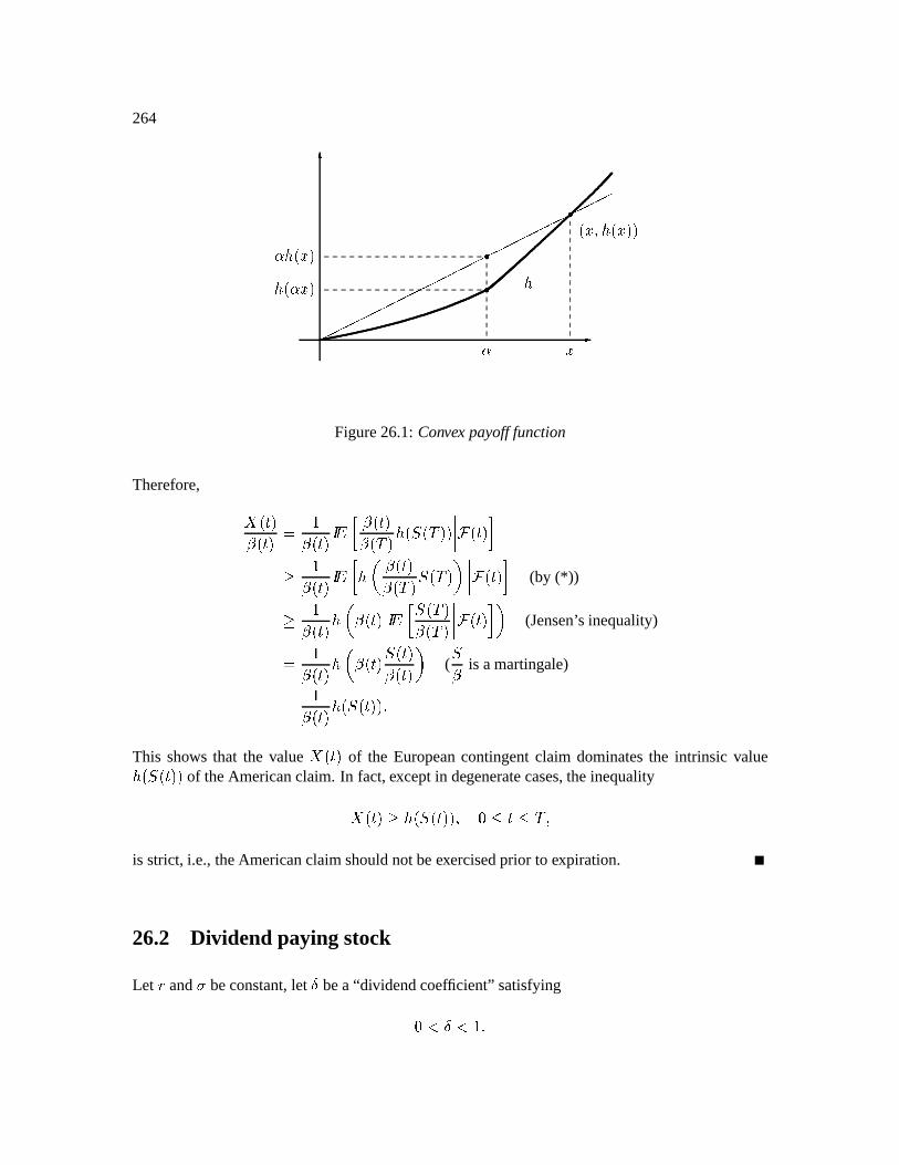
264
µ
¶
.........................................................................................................................................
...............................................................................................................
.....................................................................................................................................................
.....................................................................................
.........................................................
...............................................
.............................................
.........................................................
..................................
......... ......... ......... ......... ......... ......... ......... ......... ......... ......... ......... ......... ......... ......... ......... ......... ......... ......... ......... ...
......... ......... ......... ......... ......... ......... ......... ......... ......... ......... ......... ......... ......... ......... ......... ......... ......... ......... ......... ...
.........
.........
.........
.........
........
.
........
.
........
.
........
.
........
.
......
.........
.........
.........
.........
.........
.........
.........
.........
.........
.........
.........
.........
.........
.........
..... ok ^ éNokppkù
ééNoùñk#pùNéñok#p
Figure26.1:Convex payoff function
Therefore, Å3o pú o p V dú o p ° ú o pú oõÛ¯p éño oÇÛ¯pp o p ´ dú o p °õé ² ú o pú oõÛ¯p oÇÛ¯p ³ o p ´ (by (*)) dú o p é ² ú o p ° oõÛ¯pú oõÛ¯p o p ´³ (Jensen’s inequality)V dú o p é ² ú o p
o pú o p ³ (
ú is amartingale)V dú o p éNo
o pp fThis shows that the value Å3o p of the Europeancontingentclaim dominatesthe intrinsic valueéNo o pp of theAmericanclaim. In fact,exceptin degeneratecases,theinequalityÅ3o p éNo o pp ^ hji iuÛ ^is strict, i.e., theAmericanclaimshouldnotbeexercisedprior to expiration.
26.2 Dividend paying stock
LetZ
and [ beconstant,let bea“dividendcoefficient” satisfyinghÕl l d f
CHAPTER26. Optionsondividendpayingstocks 265
Let Û ¿ h beanexpiration time, andlet
¢ ¸eoh ^ Û¯p be the time of dividendpayment.Thestockpriceis givenby o p Vàþ oÃhp üSýí o Z q ¢\ [ \ p cu[ Ê o p ^ hji i ¢ ^o d q ;p o ¢ p üSýí o Z q ¢\ [ \ p8o q ¢ p cu[ o Ê o p q Ê o ¢ pp ^ ¢ l iÈÛ fConsideranAmericancall on this stock. At times
¸ o ¢ ^ ÛJp , it is not optimal to exercise,sothevalueof thecall is givenby theusualBlack-Scholesformulano ^ kp V kuo Æ oõÛ q ^ k#pÍp q b ~ Ï ß ~ÉõÐuo Æ ~ oõÛ q ^ k#pÍp ^ ¢ l iuÛ ^where Æ oõÛ q ^ kp V d[ Û q ° Þ kb c oõÛ q p8o Z [ \ X p ´ fAt time
¢ , immediatelyafter paymentof thedividend,thevalueof thecall isno ¢ ^ o d q ;p o ¢ pp fAt time
¢ , immediatelybeforepaymentof thedividend,thevalueof thecall is o ¢ ^ o ¢ pp ^where o ¢ ^ k#p Ve;ý ok q«b p ^ n@o ¢ ^ o d q ;pk fTheorem 2.65 For hÕi i ¢ , thevalueof theAmericancall is o ^ o pp , where o ^ kp Ve É! ~ Ï É!"%~ÉÑÐ o ¢ ^ o ¢ pp fThisfunctionsatisfiestheusualBlack-Scholesequationq Z »c# É c Z k c¦¢\ [ \ k \ S V h ^ hji i ¢ ^ k h ^(where V o ^ k#p ) with terminalcondition o ¢ ^ k#p Ve$;ý% ok q«b p ^ n@o ¢ ^ o d q ;pk#p& ^ k h ^andboundarycondition o ^ hp V h ^ hji iuÛ fThehedgingportfolio is Ämo p Vàþ o ^ o pp ^ hji i ¢ ^n o ^ o pp ^ ¢ l iuÛ fProof: We only needto show thatanAmericancontingentclaim with payoff o ¢ ^ o ¢ pp at time ¢ neednotbeexercisedbeforetime
¢ . Accordingto Theorem1.64,it sufficesto prove
1. o ¢ ^ hp V h ,
266
2. o ¢ ^ k#p is convex in k .
Sinceno ¢ ^ hp V h , wehave immediatelythat o ¢ ^ hp Ve;ý oh qÂb p ^ n@o ¢ ^ o d q ;php V h fTo provethat o ¢ ^ k#p is convex in k , weneedtoshow that no ¢ ^ o d q ;pk#p is convex is k . Obviously,ok qub p is convex in k , andthemaximumof two convex functionsis convex. Theproof of theconvexity of no ¢ ^ o d q ;pk#p in k is left asahomework problem.
26.3 Hedgingat time '(Let k V o ¢ p .CaseI: no ¢ ^ o d q ;pkp oÃk qÂb p .Theoptionneednot beexercisedat time
¢ (shouldnot beexercisedif theinequalityis strict). Wehave o ¢ ^ k#p V n@o ¢ ^ o d q ;pk#p ^Ämo ¢ p V o ¢ ^ k#p V o d q pÍn o ¢ ^ o d q ;pkp V o d q ;pÄso ¢ c p ^where Ämo ¢ c p VøÞÉ*)É!" Äso pis thenumberof sharesof stockheldby thehedgeimmediatelyafterpaymentof thedividend.Thepost-dividendpositioncanbeachievedby reinvestingin stockthedividendsreceivedon thestockheldin thehedge.Indeed,Äso ¢ c p V dd q Äso ¢ p V Äso ¢ p c d q Äso ¢ pV Äso ¢ p c ;Äso ¢ p o ¢ po d q ;p o ¢ pV
# of sharesheldwhendividendis paid c dividendsreceivedpricepersharewhendividendis reinvested
CaseII: no ¢ ^ o d q ;pk#p0l½ok q«b p .Theownerof theoptionshouldexercisebeforethedividendpaymentattime
¢ andreceive ok q b p .Thehedgehasbeenconstructedsothesellerof theoptionhas k qÂb beforethedividendpaymentat time
¢ . If theoptionis notexercised,its valuedropsfrom k q b to n@o ¢ ^ o d q ;pkp , andthesellerof theoptioncanpocketthedifferenceandcontinuethehedge.
Chapter 27
Bonds,forward contractsand futur es
Let
,+ o p ^ o pS¯hmi ieÛ bea Brownianmotion(Wienerprocess)on some o!- ^ ^/. p . Con-sideranasset,which wecall astock,whosepricesatisfiesÆ o p V Z o p o p Æ c3[ o p o p Æ + o p fHere,
Zand [ areadaptedprocesses,andwe have alreadyswitchedto the risk-neutralmeasure,
which we call
0. Assumethat every martingaleunder
0canbe representedasan integral with
respectto
+.
Definetheaccumulationfactor
ú o p VëüSýí1 ÿ É2 Z o!p Æ 43 fA zero-couponbond,maturingat time Û , pays1 at time Û andnothingbeforetime Û . Accordingto therisk-neutralpricing formula,its valueat time
¸ © h ^ Û isÊ o ^ Û¯p V ú o p ° dú oÇÛ¯p o p ´Ve ° ú o pú oõÛJp o p ´Ve 65õüSýí þ q ÿ ßÉ Z o!#p Æ o p87 f
GivenÊ o ^ Û¯p dollarsat time
, onecanconstructa portfolio of investmentin thestockandmoney
267
268
marketsothattheportfolio valueat time Û is 1 almostsurely. Indeed,for someprocess
U,Ê o ^ Û¯p V ú o p ° dú oÇÛ¯p o p ´y z |
martingaleV ú o p¯° ² dú oõÛ¯p ³ c ÿ É2 U o!#p Æ + o!p ´V ú o p¯° Ê oh ^ Û¯p c ÿ É2 U o!p Æ + o#p ´ ^ÆÊ o ^ ÛJp V Z o p ú o pJ° Ê oÃh ^ Û¯p c ÿ É2 U o!#p Æ + o!p ´ Æ c ú o p U o p Æ + o pV Z o p Ê o ^ Û¯p Æ c ú o p U o p Æ + o p fThevalueof aportfolio satisfiesÆ ÅÈo p V Äso p Æ o p c Z o p © Å3o p q Ämo p o p Æ V Z o p%Å3o p Æ c Äso p [ o p o p Æ + o p f
(*)
We set Äso p V ú o p U o p[ o p o p fIf, atany time
, Å3o p V Ê o ^ Û¯p andwe usetheportfolio Äso!p ^ imiuÛ , thenwewill haveÅÈoÇÛ¯p V Ê oõÛ ^ Û¯p V d f
IfZ o p is nonrandomfor all
, thenÊ o ^ Û¯p VëüSýí þ q ÿ ßÉ Z o!#p Æ ^Æ¬Ê o ^ Û¯p V Z o p Ê o ^ Û¯p Æ ^
i.e.,
U¤V h . Then Ä givenabove is zero.If, at time
, you aregiven
Ê o ^ ÛJp dollarsandyou alwaysinvestonly in themoney market,thenat time Û you will haveÊ o ^ Û¯p üSýíþ ÿ ßÉ Z o!p Æ V d fIfZ o p is randomfor all
, then
Uis not zero. Onegenerallyhasthreedifferentinstruments:the
stock,themoney market,andthezerocouponbond. Any two of themaresufficient for hedging,andthetwo whicharemostconvenientcandependon theinstrumentbeinghedged.
CHAPTER27. Bonds,forwardcontractsandfutures 269
27.1 Forward contracts
We continuewith the set-upfor zero-couponbonds. The Û -forward price of the stock at time ¸ © h ^ Û is the o p -measurableprice,agreeduponat time
, for purchaseof a shareof stockat
time Û , chosensotheforwardcontracthasvaluezeroat time
. In otherwords, ° dú oõÛ¯p o
oõÛ¯p q:9 o pp o p ´ V h ^ h±i iuÛ fWe solvefor
9 o p : h Ve ° dú oõÛ¯p o oõÛ¯p q:9 o pÍp o p ´Ve ° oõÛJpú oÇÛ¯p o p ´ q 9 o pú o p °ú o pú oõÛ¯p o p ´V o pú o p q 9 o pú o p Ê o ^ Û¯p f
This impliesthat 9 o p V o pÊ o ^ Û¯p fRemark 27.1(Valuevs. Forward price) The Û -forward price
9 o p is not the valueat time
of
the forwardcontract.Thevalueof thecontractat time
is zero.
9 o p is thepriceagreeduponattime
whichwill bepaidfor thestockat time Û .
27.2 Hedginga forward contract
Entera forwardcontractat time 0, i.e., agreeto pay9 oÃhp V ÎÏ 2 Ð; Ï 2 ß Ð for a shareof stockat time Û .
At timezero,thiscontracthasvalue0. At latertimes,however, it doesnot. In fact, its valueat time ¸ © h ^ Û is < o p V ú o p ° dú oõÛ¯p o oõÛ¯p q:9 ohpp o p ´V ú o p ° oõÛ¯pú oõÛJp o p ´ q=9 ohp ° ú o pú oÇÛ¯p o p ´V ú o p
o pú o p q:9 ohp Ê o ^ Û¯pV o p q:9 ohp Ê o ^ Û¯p fThissuggeststhefollowing hedgeof ashortpositionin theforwardcontract.At time0, short
9 oÃhpÛ -maturityzero-couponbonds.Thisgeneratesincome9 ohp Ê oh ^ Û¯p V ohpÊ oh ^ Û¯p Ê oÃh ^ Û¯p V ohp f
270
Buy oneshareof stock. This portfolio requiresno initial investment.Maintain this positionuntiltime Û , whentheportfolio is worth oõÛ¯p q:9 ohp Ê oõÛ ^ Û¯p V oõÛJp q:9 oÃhp fDeliver theshareof stockandreceivepayment
9 ohp .A shortpositionin the forwardcould alsobe hedgedusingthe stockandmoney market,but theimplementationof thishedgewouldrequirea term-structuremodel.
27.3 Futur econtracts
Futurecontractsaredesignedto remove therisk of defaultinherentin forwardcontracts.Throughthedevice of markingto market, thevalueof the futurecontractis maintainedat zeroat all times.Thus,eitherpartycancloseout his/herpositionatany time.
Let usfirst considerthesituationwith discretetradingdatesh Vë 2 l ¢ l f8f>f l 8>V Û fOneach
©!? ^ !? ¢ p , Z is constant,so
ú o A@ ¢ p VëüSýí1 ÿ ÉCBED "2 Z o!#p Æ 3VëüSýíGFH I @J?LK 2 Z o ? p8o ? ¢ q ? pNM OPis o A@ p -measurable.
Entera futurecontractat time
@, takingthelong position,whenthefuturepriceis Qo @ p . At timeA@ ¢ , whenthefutureprice is Qo A@ ¢ p , you receive a paymentQ o A@ ¢ p q Q o A@ p . (If thepricehas
fallen, you makethe paymentq oQo A@ ¢ p q Qo E@ pp . ) The mechanismfor receiving andmaking
thesepaymentsis themargin accountheldby thebroker.
By time Û Vë> , youhave receivedthesequenceof paymentsQo A@ ¢ p q Qo E@ p ^ Qo A@ \Sp q Qo E@ ¢ p ^ f8f8f ^ Qo > p q Qo > ~ ¢ pat times
A@ ¢ ^ E@ \ ^ f>f8f ^ > . Thevalueat time
'Vë 2 of thissequenceis
ú o p áä > ~ ¢J?/KR@ dú o !? ¢ p oCQ o !? ¢ p q Qo ? pp4 o p åè fBecauseit costsnothingto enterthe futurecontractat time
, this expressionmustbezeroalmost
surely.
CHAPTER27. Bonds,forwardcontractsandfutures 271
Thecontinuous-timeversionof thisconditionis
ú o p S5 ÿ ßÉ dú o#p Æ Qo!#p o p87 V h ^ hji iÈÛ fNotethat ú o ? ¢ p appearingin thediscrete-timeversionis o ? p -measurable,asit shouldbewhenapproximatinga stochasticintegral.
Definition 27.1 The Û -futurepriceof thestockis any o p -adaptedstochasticprocess Qo pS'hji iuÛ ^satisfying QoõÛ¯p V oõÛ¯p a.s.,and (a) 65 ÿ ßÉ dú o!p Æ Qo#p o p87 V h ^ hji iuÛ f (b)
Theorem 3.66 Theuniqueprocesssatisfying(a) and(b) isQo p Ve ° oõÛJp o p ´ ^ hji iÈÛ fProof: We first show that (b) holds if andonly if Q is a martingale. If Q is a martingale,thenT É2 ¢U ÏV Ð Æ Q o!#p is alsoamartingale,so 65 ÿ ßÉ dú o!p Æ Qo#p o p7 Vø ° ÿ É2 dú o!p Æ Qo#p o p ´ q«ÿ É2 dú o!#p Æ Qo!pV h fOntheotherhand,if (b) holds,thenthemartingaleW o p Vø 65 ÿ ß2 dú o!p Æ Qo#p o p87satisfies W o p V ÿ É2 dú o#p Æ Qo!#p c X5 ÿ ßÉ dú o!#p Æ Qo#p o pA7V ÿ É2 dú o#p Æ Qo!#p ^ hji iÈÛ fthis implies Æ W o p V dú o p Æ Q o p ^Æ Qo p V ú o p Æ W o p ^
272
andso Q is amartingale(its differentialhasnoÆ
term).
Now define Qo p Ve ° oÇÛ¯p o p ´ ^ h±i iuÛ fClearly(a) is satisfied.By thetowerproperty, Q is amartingale,so(b) is alsosatisfied.Indeed,thisQ is theonly martingalesatisfying(a).
27.4 Cashflow fr om a futur e contract
With aforwardcontract,enteredat time0, thebuyeragreesto pay9 ohp for anassetvaluedat
oÇÛ¯p .Theonly paymentis at time Û .
With a future contract,enteredat time 0, the buyer receivesa cashflow (which may at timesbenegative)betweentimes0 and Û . If hestill holdsthecontractat time Û , thenhepays
oÇÛ¯p at timeÛ for anassetvaluedat
oõÛ¯p . Thecashflow receivedbetweentimes0 and Û sumstoÿ ß2 Æ Qo!p V QoõÛJp q Q ohp V oõÛ¯p q Qohp fThus,if thefuturecontractholdertakesdeliveryat time Û , hehaspaida totalofo!Qohp q oõÛ¯pp c oõÛ¯p V Qohpfor anassetvaluedat
oõÛ¯p .27.5 Forward-futur espread
Futureprice: Qo p Ve ° oõÛJp o p ´ .Forwardprice: 9 o p V o pÊ o ^ ÛJp V o pú o p ° ¢U Ï ß Ð o p ´
fForward-futurespread:Qohp qY9 ohp Ve ª© oõÛ¯p q ohp ¢U Ï ß Ð V d Ë ¢U Ï ß Ð Ì ° ² dú oõÛ¯p ³ o
oõÛ¯pÍp q ² oõÛ¯pú oõÛ¯p ³ñ´ fIf ¢U Ï ß Ð and
oõÛ¯p areuncorrelated, Q ohp V 9 ohp f
CHAPTER27. Bonds,forwardcontractsandfutures 273
If ¢U Ï ß Ð and
oõÛ¯p arepositively correlated,thenQ ohp0i 9 ohp fThis is thecasethata rise in stockpricetendsto occurwith a fall in the interestrate. The ownerof thefuturetendsto receive incomewhenthestockpricerises,but investsit ata declininginterestrate. If the stockprice falls, the owner usuallymustmakepaymentson the future contract. Hewithdrawsfrom themoney marketto dothis justastheinterestraterises.In short,thelongpositionin the future is hurt by positive correlationbetween ¢U Ï ß Ð and
oõÛJp . The buyer of the future iscompensatedby a reductionof thefuturepricebelow theforwardprice.
27.6 Backwardation and contango
Suppose Æ o p V[Z o p Æ cu[ o p Æ + o p fDefine \ V6] ~[ ^_^+ o p V \ c + o p ,` oõÛ¯p VëüSýí q \ + oõÛJp q ¢\ \ \ Û ^ 0 o!a¯p V ÿb ` oõÛJp Æ 0 ^ òca½¸ oõÛ¯p fThen ^+ is a Brownianmotionunder
0, andÆ o p V Z o p Æ c¥[ o p Æ ^+ o p f
We have ú o p Ve %É o p V oÃhp üSýí o Z q ¢\ [ \ p cu[ + o p V oÃhp üSýí o Z q ¢\ [ \ p cu[ ^+ o p Because ¢U Ï ß Ð Ve ~ ß is nonrandom,
oõÛ¯p and ¢U Ï ß Ð areuncorrelatedunder
0. Therefore,Qo p V ^ © oÇÛ¯p o p V 9 o pV o pÊ o ^ Û¯p Ve Ï ß ~ÉÑÐ o p f
Theexpectedfuturespotpriceof thestockunder
0is oõÛ¯p V oÃhp ] ß à üSýíed q ¢\ [ \ Û c¥[ + oõÛ¯pgf Ve ] ß oÃhp f
274
Thefuturepriceat time h is Q ohp Ve ß ohp fIf
Z ¿ Z , then Qohpal oõÛ¯p f Thissituationis callednormalbackwardation(seeHull). If
Z l Z ,then Qohpa¿ oõÛ¯p . This is calledcontango.
Chapter 28
Term-structure models
Throughoutthisdiscussion,
+ o pS'hÕi i¥Û ` is a Brownianmotiononsomeprobabilityspaceo!- ^ ^h. p , and
9 o pSahji iÂÛ ` is thefiltration generatedby
+.
Supposewe aregivenanadaptedinterestrateprocess
Z o pS'hji iuÛ ` . We definetheaccumu-lation factor ú o p VëüSýí 1 ÿ É2 Z o#p Æ 3 ^ h±i iÈÛ ` fIn a term-structuremodel,we takethezero-couponbonds(“zeroes”)of variousmaturitiesto betheprimitiveassets.We assumethesebondsaredefault-freeandpay$1at maturity. For hÕi i3Û iÛ ` , let Ê o ^ Û¯p V priceat time
of thezero-couponbondpaying$1at time Û .
Theorem 0.67(FundamentalTheorem of AssetPricing) A termstructure modelis freeof arbi-trageif andonly if there is a probability measure ^ 0 on - (a risk-neutral measure) with thesameprobability-zerosetsas
0(i.e., equivalentto
0), such that for each Ûe¸»oh ^ Û ` , theprocessÊ o ^ ÛJpú o p ^ hji iuÛ ^
is a martingaleunder ^ 0 .
Remark 28.1 WeshallalwayshaveÆÊ o ^ Û¯p V[Z o ^ ÛJp Ê o ^ Û¯p Æ c#i o ^ Û¯p Ê o ^ Û¯p Æ + o p ^ hji iÈÛ ^for somefunctions
Z o ^ Û¯p and i o ^ Û¯p . ThereforeÆ ² Ê o ^ Û¯pú o p ³ V Ê o ^ Û¯p Æ ² dú o p ³ c dú o p Æ¬Ê o ^ Û¯pV ©jZ o ^ Û¯p qÂZ o p Ê o ^ Û¯pú o p Æ c#i o ^ Û¯p Ê o ^ Û¯pú o p Æ + o p ^275
276
so
0is a risk-neutralmeasureif andonly if
Z o ^ Û¯p , themeanrateof returnofÊ o ^ Û¯p under
0, is
theinterestrateZ o p . If themeanrateof returnof
Ê o ^ ÛJp under
0is not
Z o p ateachtime
andfor
eachmaturity Û , we shouldchangeto a measure
0underwhich themeanrateof returnis
Z o p . Ifsucha measuredoesnotexist, thenthemodeladmitsanarbitrageby tradingin zero-couponbonds.
28.1 Computing arbitrage-fr eebond prices: first method
Begin with a stochasticdifferentialequation(SDE)Æ Å3o p Vlk o ^ Å3o pp Æ c#m o ^ Å3o pÍp Æ + o p fThe solution Å3o p is the factor. If we want to have n -factors,we let
+be an n -dimensional
Brownianmotionandlet Å bean n -dimensionalprocess.We let theinterestrateZ o p bea function
of Å3o p . In theusualone-factormodels,we takeZ o p to be Å3o p (e.g.,Cox-Ingersoll-Ross,Hull-
White).
Now that we have an interestrateprocess
Z o pSh«i i¦Û ` , we definethe zero-couponbondpricesto be Ê o ^ Û¯p V ú o p ° dú oõÛ¯p o p ´Ve S5ÑüSýíþ qsÿ ßÉ Z o!p Æ o p87 ^ hji iuÛ½iuÛ ` fWe showedin Chapter27 thatÆÊ o ^ Û¯p V Z o p Ê o ^ Û¯p Æ c ú o p U o p Æ + o pfor someprocess
U. Since
Ê o ^ ÛJp hasmeanrateof returnZ o p under
0,
0is arisk-neutralmeasure
andthereis noarbitrage.
28.2 Someinterest-ratedependentassets
Coupon-payingbond: Payments
0 ¢ ^ 0 \ ^ f8f>f ^ 0 > at times Û ¢ ^ Û]\ ^ f8f8f ^ Û > . Priceat time
isJ @ ô É ß B 04@ Ê o ^ Û @ p f
Call option on a zero-couponbond: Bond maturesat time Û . Option expiresat time Û ¢ l Û .Priceat time
is
ú o p ° dú oõÛ ¢ p o Ê oõÛ ¢ ^ Û¯p q«b p o p ´ ^ h±i iuÛ ¢ f
CHAPTER28. Term-structuremodels 277
28.3 Terminology
Definition 28.1(Term-structure model) Any mathematicalmodelwhichdetermines,at leastthe-oretically, thestochasticprocesses Ê o ^ ÛJp ^ hji iuÛ ^for all Û½¸Âoh ^ Û ` .Definition 28.2(Yield to maturity) For hui i Û i Û ` , the yield to maturity Ôso ^ Û¯p is the o p -measurablerandom-variablesatisfyingÊ o ^ ÛJp üSýíJ oõÛ q pPÔ o ^ ÛJp V d ^or equivalently, ÔWo ^ ÛJp V q dÛ q ÞoN Ê o ^ Û¯p fDetermining Ê o ^ Û¯p ^ hji iÈÛÀiuÛ ` ^is equivalentto determining ÔWo ^ Û¯p ^ hji iÈÛÀiuÛ ` f28.4 Forward rate agreement
Let hÕi i¥ÛÀl¥Û c#p i¥Û ` begiven.Supposeyou wantto borrow $1at time Û with repayment(plusinterest)at time Û cp , ataninterestrateagreeduponat time
. To synthesizea forward-rate
agreementto do this, at time
buy a Û -maturityzeroandshort
; Ï É! ß Ð; Ï É! ß Rq Ð oõÛ cGp p -maturityzeroes.Thevalueof thisportfolio at time
isÊ o ^ Û¯p q Ê o ^ Û¯pÊ o ^ Û c#p p Ê o ^ Û c#p p V h f
At time Û , you receive $1 from the Û -maturity zero. At time Û crp , you pay $; Ï É! ß Ð; Ï É! ß Rq Ð . The
effective interestrateon thedollaryou receive at time Û is
¹ o ^ Û ^ Û c#p p givenbyÊ o ^ Û¯pÊ o ^ Û cp p VëüSýí p ¹ o ^ Û ^ Û c#p p ^or equivalently, ¹ o ^ Û ^ Û c#p p V q ÞoN Ê o ^ Û csp p q Þ Ê o ^ ÛJpp fTheforward rate is t o ^ ÛJp VëÞq ) 2 ¹ o ^ Û ^ Û cp p V qXuu Û ÞoN Ê o ^ Û¯p f (4.1)
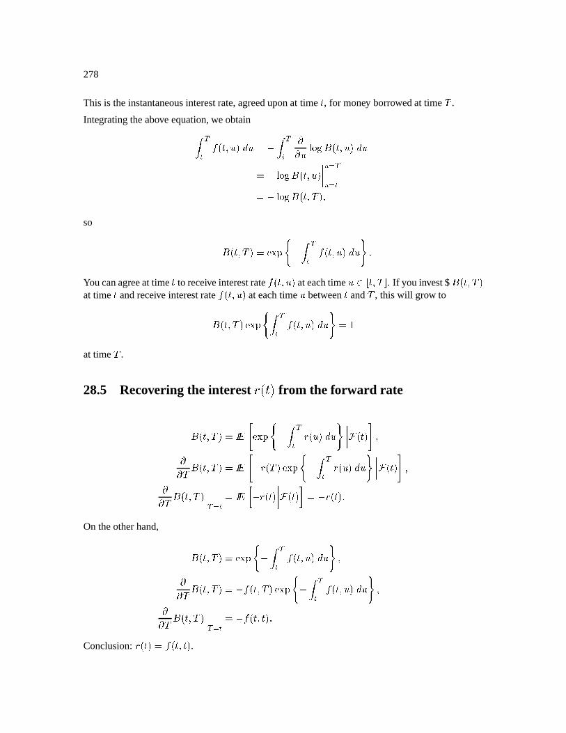
278
This is theinstantaneousinterestrate,agreeduponat time
, for money borrowedat time Û .
Integratingtheabove equation,weobtainÿ ßÉt o ^ p Æ V q ÿ ßÉ uu ÞoN Ê o ^ #p Æ V q ÞoN Ê o ^ #p V
K ßV K ÉV q ÞoN Ê o ^ Û¯p ^so Ê o ^ ÛJp VëüSýí þ qsÿ ßÉ
t o ^ #p Æ fYoucanagreeat time
to receiveinterestrate
t o ^ p ateachtime ¸ © ^ Û . If youinvest$Ê o ^ Û¯p
at time
andreceive interestrate
t o ^ #p ateachtime between
and Û , thiswill grow toÊ o ^ ÛJp üSýíïþ ÿ ßÉ
t o ^ p Æ V dat time Û .
28.5 Recovering the interest vw'x fr om the forward rate
Ê o ^ Û¯p Ve X5ÑüSýíþ qsÿ ßÉ Z o!p Æ o p87 ^uu Û Ê o ^ Û¯p Ve 5 q Z oõÛ¯p üSýí þ q ÿ ßÉ Z o!p Æ o p 7 ^uu Û Ê o ^ Û¯p ß K É Ve ° q Z o py o p ´ V q Z o p fOntheotherhand, Ê o ^ Û¯p VëüSýíþ qsÿ ßÉ
t o ^ p Æ ^uu Û Ê o ^ Û¯p V q t o ^ Û¯p üSýíþ qsÿ ßÉt o ^ p Æ ^uu Û Ê o ^ Û¯p ß K É V q t o ^ p f
Conclusion:Z o p V t o ^ p .
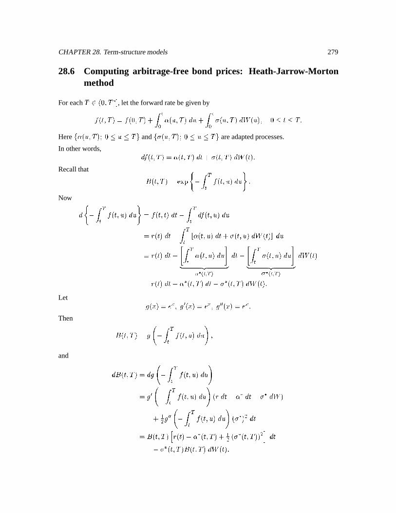
CHAPTER28. Term-structuremodels 279
28.6 Computing arbitrage-fr eebond prices: Heath-Jarr ow-Mortonmethod
For eachÛ½¸Âoh ^ Û ` , let theforwardratebegivenbyt o ^ Û¯p V t oh ^ Û¯p c ÿ É2 ù0o! ^ Û¯p Æ c ÿ É2 [ o! ^ Û¯p Æ + o!#p ^ hji iÈÛ fHere
ù0o! ^ Û¯pSñhjisiÈÛ and
[ o! ^ Û¯p NhÕis¤iuÛ areadaptedprocesses.
In otherwords, Æ t o ^ ÛJp V ù o ^ ÛJp Æ cu[ o ^ Û¯p Æ + o p fRecallthat Ê o ^ Û¯p VëüSýíþ qmÿ ßÉ
t o ^ p Æ fNow Æ þ q ÿ ßÉ
t o ^ p Æ V t o ^ p Æ q ÿ ßÉ Æ t o ^ p Æ V Z o p Æ qÂÿ ßÉ © ù o ^ p Æ cu[ o ^ #p Æ + o p Æ V Z o p Æ q 5 ÿ ßÉ ù0o ^ #p Æ z7y z | Ó Ï É! ß ÐÆ q 5 ÿ ßÉ [ o ^ p Æ |7y z |[ Ó Ï É ß Ð
Æ + o pV Z o p Æ q ù ` o ^ Û¯p Æ q [ ` o ^ Û¯p Æ + o p fLet oÃk#p Ve ^ ¡Çokp Ve ^ ¡ ¡Çokp Ve fThen Ê o ^ Û¯p V ~ q ÿ ßÉ
t o ^ #p Æ ^and Æ¬Ê o ^ Û¯p V Æ ~ q ÿ ßÉ
t o ^ #p Æ V ¡ ~ q ÿ ßÉt o ^ #p Æ o Z Æ q ù ` Æ q [ ` Æ + pc ¢\ ¡ ¡ ~ qsÿ ßÉ
t o ^ #p Æ Âo [ ` p \ Æ V Ê o ^ ÛJp Z o p q ù ` o ^ Û¯p c¦¢\ o [ ` o ^ Û¯pp \ Æ q [ ` o ^ Û¯p Ê o ^ Û¯p Æ + o p f
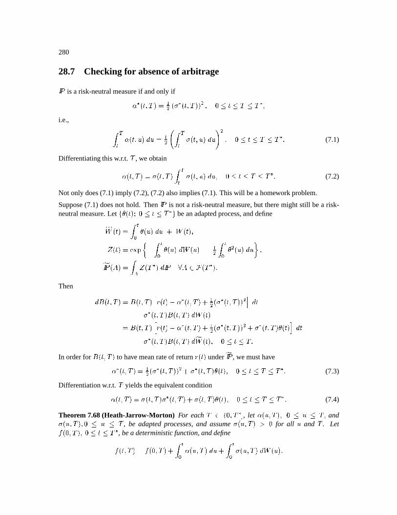
280
28.7 Checking for absenceof arbitrage 0is a risk-neutralmeasureif andonly ifù ` o ^ Û¯p V ¢\ o [ ` o ^ Û¯pp \ ^ hji iuÛeiÈÛ `;^
i.e., ÿ ßÉ ù0o ^ #p Æ V ¢\ ~ ÿ ßÉ [ o ^ #p Æ \ ^ hji iuÛ½iuÛ ` f (7.1)
Dif ferentiatingthisw.r.t. Û , we obtainù0o ^ Û¯p V [ o ^ Û¯p ÿ ßÉ [ o ^ #p Æ ^ hji iuÛ½iuÛ ` f (7.2)
Not only does(7.1) imply (7.2),(7.2)alsoimplies(7.1). Thiswill bea homework problem.
Suppose(7.1)doesnot hold. Then
0is not a risk-neutralmeasure,but theremight still bea risk-
neutralmeasure.Let
\o pSah±i iuÛ ` beanadaptedprocess,anddefine^+ o p V ÿ É2 \o!#p Æ c + o p ^` o p VëüSýí 1 q ÿ É2 \o!p Æ + o!p q ¢\ ÿ É2 \ \ o!#p Æ 3 ^^ 0 oa¯p V ÿ b ` oõÛ ` p Æ 0 òca½¸ oõÛ ` p fThen ÆÊ o ^ Û¯p V Ê o ^ Û¯p Z o p q ù ` o ^ Û¯p c¦¢\ o [ ` o ^ ÛJpp \ Æ q [ ` o ^ Û¯p Ê o ^ ÛJp Æ + o pV Ê o ^ Û¯p Z o p q ù ` o ^ Û¯p c¦¢\ o [ ` o ^ ÛJpp \ c¥[ ` o ^ ÛJp/\o p Æ q [ ` o ^ Û¯p Ê o ^ ÛJp Æ ^+ o p ^ h±i iÈÛ fIn orderfor
Ê o ^ Û¯p to havemeanrateof returnZ o p under ^ 0 , wemusthaveù ` o ^ ÛJp V ¢\ o [ ` o ^ Û¯pp \ c¥[ ` o ^ Û¯p/\o p ^ hji iÈÛÀiuÛ ` f (7.3)
Dif ferentiationw.r.t. Û yieldstheequivalentconditionù o ^ ÛJp V [ o ^ Û¯p [ ` o ^ ÛJp c¥[ o ^ Û¯p/\o p ^ hji i»ÛÀiuÛ ` f (7.4)
Theorem 7.68(Heath-Jarrow-Morton) For each Û ¸roh ^ Û ` , let ù0o! ^ Û¯p ^ hëi iYÛ ^ and[ o! ^ Û¯p ^ heiriûÛ , be adaptedprocesses,and assume[ o! ^ Û¯p»¿ h for all and Û . Lett oh ^ Û¯p ^ hji iÂÛ ` , bea deterministicfunction,anddefinet o ^ Û¯p V t oÃh ^ Û¯p c ÿ É2 ù o ^ ÛJp Æ c ÿ É2 [ o! ^ Û¯p Æ + o!p f
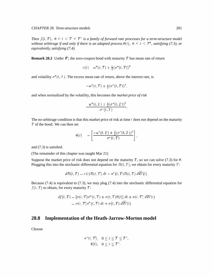
CHAPTER28. Term-structuremodels 281
Then
t o ^ Û¯p ^ hgi i½Û i½Û ` is a family of forward rate processesfor a term-structure modelwithoutarbitrage if andonly if there is an adaptedprocess\o p ^ hsi i½Û ` , satisfying(7.3),orequivalently, satisfying(7.4).
Remark 28.2 Under
0, thezero-couponbondwith maturity Û hasmeanrateof returnZ o p q ù ` o ^ ÛJp c£¢\ o [ ` o ^ Û¯pp \
andvolatility [ ` o ^ Û¯p . Theexcessmeanrateof return,above theinterestrate,isq ù ` o ^ Û¯p c ¢\ o [ ` o ^ ÛJpp \ ^andwhennormalizedby thevolatility, thisbecomesthemarketpriceof riskq ù ` o ^ Û¯p c£¢\ o [ ` o ^ ÛJpp \[ ` o ^ Û¯p fTheno-arbitrageconditionis thatthismarketpriceof risk at time
doesnotdependonthematurityÛ of thebond.We canthenset\o p V q 5 q ù ` o ^ Û¯p c£¢\ o [ ` o ^ ÛJpp \[ ` o ^ Û¯p 7 ^
and(7.3)is satisfied.
(Theremainderof thischapterwastaughtMar 21)
Supposethe marketpriceof risk doesnot dependon the maturity Û , so we cansolve (7.3) for \ .Pluggingthis into thestochasticdifferentialequationfor
Ê o ^ Û¯p , weobtainfor everymaturity Û :Æ¬Ê o ^ Û¯p V Z o p Ê o ^ Û¯p Æ q [ ` o ^ Û¯p Ê o ^ Û¯p Æ ^+ o p fBecause(7.4) is equivalentto (7.3),we mayplug (7.4) into thestochasticdifferentialequationfort o ^ Û¯p to obtain,for everymaturity Û :Æ t o ^ Û¯p V © [ o ^ Û¯p [ ` o ^ Û¯p cu[ o ^ Û¯p/\o p Æ c3[ o ^ Û¯p Æ + o pV [ o ^ Û¯p [ ` o ^ Û¯p Æ cu[ o ^ Û¯p Æ ^+ o p f28.8 Implementation of the Heath-Jarr ow-Morton model
Choose [ ` o ^ Û¯p ^ hji iuÛÀiuÛ ` ^\o p ^ hji iuÛ ` f
282
Thesemaybestochasticprocesses,but areusuallytakento bedeterministicfunctions.Defineù0o ^ Û¯p V [ o ^ Û¯p [ ` o ^ Û¯p c3[ o ^ Û¯p/\o p ^^+ o p V ÿ É2 \o#p Æ c + o p ^` o p VëüSýí 1 qsÿ É2 \o!#p Æ + o!#p q ¢\ ÿ É2 \ \ o!#p Æ 3 ^^ 0 o!aJp V ÿ b ` oõÛ ` p Æ 0 òca½¸ oõÛ ` p fLet
t oh ^ ÛJp ^ hjiuÛ½iuÛ ` ^ bedeterminedby themarket;recallfrom equation(4.1):t oh ^ Û¯p V q uu Û ÞoN Ê oh ^ Û¯p ^ hjiuÛeiuÛ ` fThen
t o ^ Û¯p for hÕi iuÛ is determinedby theequationÆ t o ^ Û¯p V [ o ^ ÛJp [ ` o ^ Û¯p Æ c3[ o ^ Û¯p Æ ^+ o p ^ (8.1)
thisdeterminestheinterestrateprocessZ o p V t o ^ p ^ hji iuÛ ` ^ (8.2)
andthenthezero-couponbondpricesaredeterminedby theinitial conditionsÊ oh ^ Û¯p ^ hmiÀÛ iÛ ` , gottenfrom themarket,combinedwith thestochasticdifferentialequationÆ¬Ê o ^ Û¯p V Z o p Ê o ^ Û¯p Æ q [ ` o ^ Û¯p Ê o ^ Û¯p Æ ^+ o p f (8.3)
Becauseall pricingof interestratedependentassetswill bedoneundertherisk-neutralmeasure
0,
underwhich ^+ is a Brownianmotion,we have written (8.1) and(8.3) in termsof ^+ ratherthan+. Writtenthisway, it is apparentthatneither\o p nor ù0o ^ Û¯p will entersubsequentcomputations.
Theonly processwhichmattersis [ o ^ Û¯p ^ h±i iuÛeiuÛ ` , andtheprocess[ ` o ^ Û¯p V ÿ ßÉ [ o ^ #p Æ ^ h±i iÈÛeiuÛ ` ^ (8.4)
obtainedfrom [ o ^ Û¯p .From(8.3)we seethat [ ` o ^ Û¯p is thevolatility at time
of thezerocouponbondmaturingat timeÛ . Equation(8.4)implies [ ` oõÛ ^ Û¯p V h ^ hjiuÛeiuÛ ` f (8.5)
This is becauseÊ oõÛ ^ Û¯p V d andsoas
approachesÛ (from below), thevolatility in
Ê o ^ Û¯p mustvanish.
In conclusion,to implementtheHJM model,it sufficesto havetheinitial marketdataÊ oh ^ Û¯p ^ hÕiÛÀi»Û ` ^ andthevolatilities [ ` o ^ Û¯p ^ hÕi iuÛeiuÛ ` f
CHAPTER28. Term-structuremodels 283
We requirethat [ ` o ^ Û¯p bedifferentiablein Û andsatisfy(8.5). We canthendefine[ o ^ Û¯p V uu Û [ ` o ^ ÛJp ^and(8.4)will besatisfiedbecause[ ` o ^ Û¯p V [ ` o ^ Û¯p q [ ` o ^ p V ÿ ßÉ uu [ ` o ^ #p Æ fWe thenlet ^+ bea Brownianmotionundera probabilitymeasure
0, andwe let
Ê o ^ Û¯p ^ hÕi iÛ i½Û ` , begivenby (8.3), whereZ o p is givenby (8.2) and
t o ^ Û¯p by (8.1). In (8.1) we usetheinitial conditions
t oh ^ Û¯p V q uu Û ÞoN Ê oh ^ Û¯p ^ hjiuÛeiuÛ ` fRemark 28.3 It is customaryin the literatureto write
+ratherthan ^+ and
0ratherthan ^ 0 ,
so that
0is the symbol usedfor the risk-neutralmeasureandno referenceis ever madeto the
marketmeasure.Theonlyparameterwhichmustbeestimatedfrom themarketis thebondvolatility[ ` o ^ Û¯p , andvolatility is unaffectedby thechangeof measure.

284
Chapter 29
Gaussianprocesses
Definition 29.1(GaussianProcess)A GaussianprocessÅ3o p , J h , is a stochasticprocesswiththepropertythatfor every setof times hji ¢ i \¯i f8f8f i > , thesetof randomvariablesÅ3o ¢ p ^ ÅÈo \p ^ f8f>f ^ Å3o > pis jointly normallydistributed.
Remark 29.1 If Å is aGaussianprocess,thenits distributionis determinedby its meanfunction o p Ve Å3o pandits covariancefunctioni o! ^ p Ve ª© o*Å3o!8p q o!8pp4¬oÇÅÈo p q o pÍp fIndeed,thejoint densityof Å3o ¢ p ^ f8f8f ^ Å3o > p is 0 Å3o ¢ p0¸ Æ k ¢ ^ f8f>f ^ Å3o > p0¸ Æ k > V do X p >, \ üc üSýíed q ¢\ o q o8pp ~c ¬o q o8ppEf Æ k ¢ f8f8f Æ k > ^where
is thecovariancematrixuV áãããä i o ¢ ^ ¢ p i o ¢ ^ \ p f>f8f i o ¢ ^ > pi o \ ^ ¢ p i o \ ^ \Sp f>f8f i o \ ^ > pf8f>f f>f8f f>f8f f>f8fi o > ^ ¢ p i o > ^ \Sp f>f8f i o > ^ > p å æææè is therow vector
© k ¢ ^ k\ ^ f8f8f ^ k > , is therow vector
© ¢ ^ \ ^ f8f>f ^ > , and o8p V © o ¢ p ^ o \,p ^ f>f8f ^ o > p .Themomentgeneratingfunctionis üSýí þ >J@K ¢ @ Å3o A@ p VëüSýíedR o8p c¦¢\ f ^where
sV © ¢ ^ \ ^ f8f>f ^ > .285
286
29.1 An example:Brownian Motion
Brownianmotion
+is aGaussianprocesswith o p V h and i o ^ p V Ü . Indeed,if hji i ,
then i o! ^ p Ve 3©j+ o!8p + o p Ve o+ o8pNo + o p q + o!8pp c + \ o!>p Ve + o!>p f o + o p q + o!8pp c + \ o!>pVe + \ o!8pV Ü fTo prove thataprocessis Gaussian,onemustshow that Å3o ¢ p ^ f>f8f ^ ÅÈo > p haseitheradensityor amomentgeneratingfunctionof theappropriateform. We shallusethem.g.f.,andshallcheata bitby consideringonly two times,whichwe usuallycall and
. We will wantto show that »üSýíJ ¢ Å3o!8p c \ ÅÈo p VëüSýíþ ¢ ¢ c \ \ c ¢\ © ¢ \ 5 [ ¢¢ [ ¢ \[ \ ¢ [ \Í\ 7 5 ¢#\ 7 f
Theorem 1.69(Integral w.r.t. a Brownian) Let
+ o p bea Brownianmotionand o p a nonran-domfunction.Then Å3o p V ÿ É2 o#p Æ + o!pis a Gaussianprocesswith o p V h andi o! ^ p V ÿ É2 \ o!p Æ fProof: (Sketch.)We have Æ Å V Æ + fTherefore, Æ VJÏ Ð V VJÏ Ðo!>p Æ + o!>p c ¢\ \ VJÏ Ð \ o!8p Æ ^ VJÏ Ð Ve VJÏ 2 Ð c ÿ 2 V¯Ïo Ð8oÃn¬p Æ + oÃn¬py z, |
Martingale
c ¢\ \ ÿ 2 VJÏ Ð8 \ on¬p Æ n ^ j VJÏ Ð V dwc¦¢\ \ ÿ2 \ on¬p j VJÏ Ð Æ n ^ÆÆ j VJÏ Ð V ¢\ \ \ o8p j V¯Ï Ð ^ j VJÏ Ð Ve VJÏ 2 Ð üSýí 1 ¢\ \ ÿ2 \ onp Æ n 3 (1.1)VëüSýí1 ¢\ \ ÿ2 \ on¬p Æ nR3 fThisshowsthat Å3o!>p is normalwith mean0 andvariance
T 2 \ on¬p Æ n .
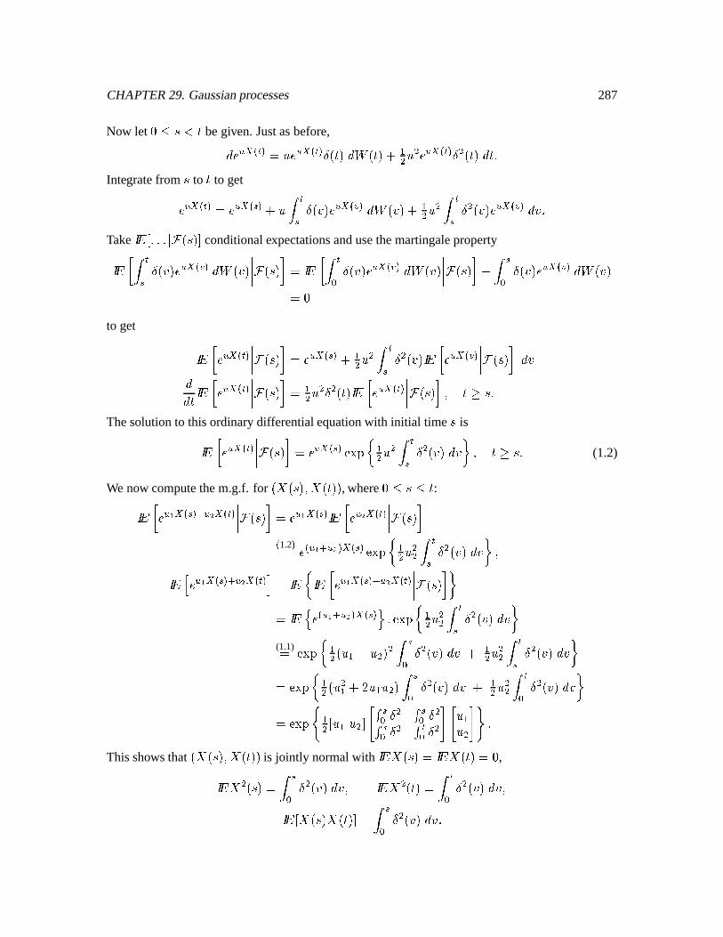
CHAPTER29. Gaussianprocesses 287
Now let hÕisl begiven.Justasbefore,Æ VJÏ ÉÑÐ V V¯Ï ÉÑÐ o p Æ + o p c¦¢\ \ V¯Ï ÉÑÐ \ o p Æ fIntegratefrom to
to get VJÏ ÉÑÐ Ve VJÏ Ð c ÿ É onp VJÏo Ð Æ + oÃn¬p c ¢\ \ ÿ É \ onp VJÏo Ð Æ n f
Take
© f8f>f¡ o8p conditionalexpectationsandusethemartingaleproperty ° ÿ É oÃn¬p VJÏ Ð Æ + oÃn¬p o8p ´ Vë ° ÿ É2 onp VJÏo Ð Æ + oÃn¬p o8p ´ q ÿ2 onp VJÏo Ð Æ + onpV hto get ° VJÏ ÉÑÐ o8p ´ Vë VJÏ Ð c¦¢\ \ ÿ É \ onp ° VJÏo Ð o!8p ´ Æ nÆÆ ° VJÏ ÉÑÐ o8p ´ V ¢\ \ \ o p ° VJÏ ÉÑÐ o!>p ´ ^ 0 fThesolutionto thisordinarydifferentialequationwith initial time is ° VJÏ ÉÑÐ o!>p ´ Ve VJÏ Ð üSýí1 ¢\ \ ÿ É \ onp Æ nc3 ^ f (1.2)
We now computethem.g.f. for oõÅ3o!>p ^ Å3o pp , whereh±i i : ° V " JÏ Ð V¢AJÏ ÉÑÐ o8p ´ Ve V " ¯Ï Ð ° V¢E¯Ï ÉÑÐ o!8p ´Ï 1.2ÐV ÏoV " V¢ Ð JÏ Ð üSýí1 ¢\ \\ ÿ É \ onp Æ nR3 ^ ¦ V " JÏ Ð V¢AJÏ ÉÑÐ Ve 1 ° V " JÏ Ð V¢/JÏ ÉÑÐ o!8p ´ 3Ve sd# ÏoV " V¢ Ð JÏ ÐEf f üSýí%1 ¢\ \\ ÿ É \ on¬p Æ nR3(1.1)V üSýí1 ¢\ o! ¢ c \Sp \ ÿ£2 \ onp Æ n c ¢\ \\ ÿ É \ on¬p Æ nR3VëüSýí1 ¢\ o \ ¢ c X ¢ \Sp ÿ£2 \ onp Æ n c ¢\ \\ ÿ É2 \ onp Æ nR3VëüSýíþ ¢\ © ¢ #\ 5 T 2 \ T 2 \T 2 \ T É2 \ 7 5 ¢#\ 7 f
Thisshowsthat oÇÅÈo8p ^ ÅÈo pp is jointly normalwith
Å3o!8p Ve Å3o p V h , Å \ o!>p V ÿ2 \ onp Æ n ^ Å \ o p V ÿ É2 \ onp Æ n ^ © Å3o!8p%Å3o p V ÿ2 \ on¬p Æ n f
288
Remark 29.2 The hard part of the above argument,and the reasonwe usemomentgeneratingfunctions,is to prove thenormality. Thecomputationof meansandvariancesdoesnot requiretheuseof momentgeneratingfunctions.Indeed,Å3o p V ÿ É2 o#p Æ + o!pis amartingaleand Å3ohp V h , so o p Vø ÅÈo p V h ò 0 h fFor fixed h , Å \ o!>p V ÿ2 \ oÃn¬p Æ nby theIto isometry. For hjisi , © Å3o!>p8o*Å3o p q Å3o!8pÍp Vø ° G1 Å3o!8p8oÅ3o p q Å3o!>pp o!8p¤3 ´Vø áãããä ÅÈo8p ² ° ÅÈo p o!>p ´ q Å3o!8p ³y z |2 å æææèV h fTherefore, © Å3o!>p%Å3o p Vø © Å3o!>p8o*Å3o p q Å3o!8pÍp c Å \ o!>p Vø Å \ o!>p V ÿ£2 \ oÃn¬p Æ n fIf wereastochasticproess,theIto isometrysays Å \ o!>p V ÿ 2 \ on¬p Æ nandthesameargumentusedaboveshowsthatfor hji i , © Å3o!>p%Å3o p Ve Å \ o!8p V ÿ¥2 \ onp Æ n fHowever, when is stochastic,Å is not necessarilya Gaussianprocess,so its distribution is notdeterminedfrom its meanandcovariancefunctions.
Remark 29.3 When is nonrandom,Å3o p V ÿ É2 o#p Æ + o!pis alsoMarkov. Weprovedthisbefore,but noteagainthattheMarkov propertyfollowsimmediatelyfrom (1.2).Theequation(1.2)saysthatconditionedon o!>p , thedistributionof Å3o p dependsonlyon Å3o!8p ; in fact, Å3o p is normalwith meanÅÈo8p andvariance
T É \ oÃn¬p Æ n .
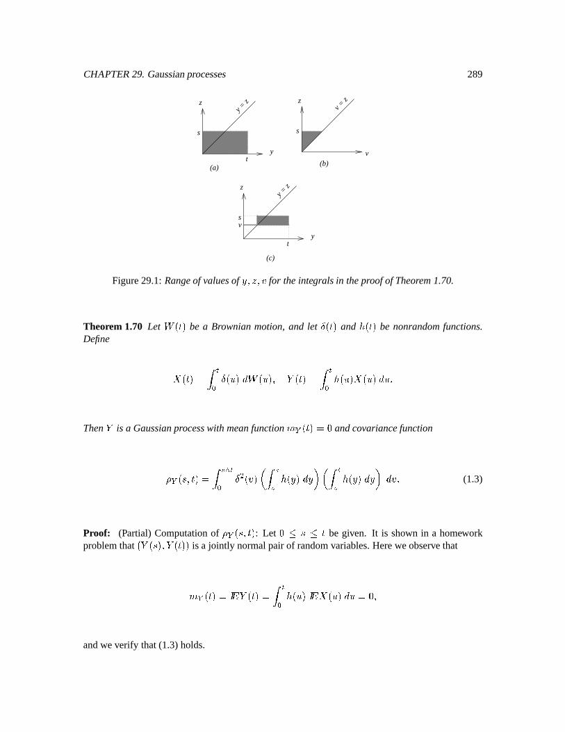
CHAPTER29. Gaussianprocesses 289
yt
y =
zz
s
z
s
v =
z
v
y
z
t
s
y =
z
v
(a) (b)
(c)
Figure29.1:Rangeof valuesof ¦ ^§^ n for theintegrals in theproofof Theorem1.70.
Theorem 1.70 Let
+ o p be a Brownianmotion,and let o p and éNo p be nonrandomfunctions.Define
ÅÈo p V ÿ É2 o!#p Æ + o#p ^ Ô¤o p V ÿ É2 éño!#pPÅÈo#p Æ fThenÔ is a Gaussianprocesswith meanfunction ©¨ o p V h andcovariancefunction
i ¨ o! ^ p V ÿ 8 É2 \ onp ² ÿ éNo!¦p Æ ¦ ³ ² ÿ É éNo¦¬p Æ ¦ ³ Æ n f (1.3)
Proof: (Partial) Computationof iz¨ o! ^ p : Let hÂi6 i be given. It is shown in a homework
problemthat oõÔso!8p ^ Ôªo pp is a jointly normalpairof randomvariables.Hereweobserve that
©¨ o p Ve ÔWo p V ÿ É2 éNo!p Å3o!#p Æ V h ^andweverify that(1.3)holds.
290
We have i ¨ o! ^ p Ve 3© Ô¤o!8pPÔWo p Ve ° ÿ£2 éNo!¦p%Å3o!¦p Æ ¦ fÿ É2 éño § p%Å3o § p Æ § ´Ve ÿ 2 ÿ É2 éNo!¦péNo § p%Å3o!¦p%Å3o § p Æ ¦ Æ §V ÿ2 ÿ É2 éNo!¦péño § p È© Å3o!¦¬pPÅÈo § p Æ ¦ Æ §V ÿ 2 ÿ É2 éNo!¦péño § p ÿ©ª N«2 \ onp Æ n Æ ¦ Æ §V ÿ2 ÿ É« éNo!¦péño § p ² ÿ«2 \ oÃn¬p Æ n ³ Æ ¦ Æ §c ÿ£2 ÿ¥ª éNo!¦péño § p ² ÿ ª2 \ oÃn¬p Æ n ³ Æ § Æ ¦ (SeeFig. 29.1(a))V ÿ2 éño § p ² ÿ É« éNo¦¬p Æ ¦ ³ ² ÿ£«2 \ onp Æ n ³ Æ §c ÿ 2 éNo!¦p ² ÿ ª éNo § p Æ § ³ ² ÿª2 \ on¬p Æ n ³ Æ ¦V ÿ 2 ÿ «2 éNo § p/ \ on¬p ² ÿ É« éNo¦¬p Æ ¦ ³ Æ n Æ §c ÿ£2 ÿ ª2 éNo!¦p/ \ oÃn¬p ² ÿª éño § p Æ § ³ Æ n Æ ¦V ÿ2 ÿ éño § p/ \ onp ² ÿ É« éño!¦¬p Æ ¦ ³ Æ § Æ nc ÿ£2 ÿ¥ éNo!¦p/ \ on¬p ² ÿª éño § p Æ § ³ Æ ¦ Æ n (SeeFig. 29.1(b))V ÿ2 \ onp ² ÿ ÿ É« éño!¦¬pÍéNo § p Æ ¦ Æ § ³ Æ nc ÿ£2 \ oÃn¬p ² ÿ ÿª éño!¦¬pÍéNo § p Æ § Æ ¦ ³ Æ nV ÿ2 \ onp ² ÿ ÿ É éño!¦¬pÍéNo § p Æ ¦ Æ §;³ Æ n (SeeFig. 29.1(c))V ÿ 2 \ onp ² ÿ éNo!¦p Æ ¦ ³ ² ÿ É éño § p Æ § ³ Æ nV ÿ2 \ onp ² ÿ éNo!¦p Æ ¦ ³ ² ÿ É éño!¦¬p Æ ¦ ³ Æ nRemark 29.4 Unlike the processÅ3o p V T É2 o!p Æ + o!#p , the processÔso p V T É2 Å3o!p Æ is
CHAPTER29. Gaussianprocesses 291
neitherMarkov noramartingale.For hjil , ª© Ôso p o8p V ÿ2 éNo!p%Å3o!#p Æ c ° ÿ É éNo!p%Å3o!#p Æ o!>p ´V Ôso!>p c ÿ É éNo!p © Å3o!p o!8p Æ V Ôso!>p c ÿ É éNo!p%Å3o!8p Æ V Ôso!>p c Å3o!8p ÿ É éNo!p Æ ^wherewe have usedthefact that Å is a martingale.Theconditionalexpectation
© ÔWo p o!8p isnotequalto Ô¤o!8p , nor is it a functionof Ô¤o!8p alone.

292
Chapter 30
Hull and White model
Consider Æ Z o p V où0o p q ú o p Z o pp Æ cu[ o p Æ + o p ^whereù o p , ú o p and [ o p arenonrandomfunctionsof
.
We cansolve thestochasticdifferentialequation.Setb o p V ÿ É2 ú o!p Æ fThen Æ±Ë g¬ Ï ÉÑÐ Z o p%Ì Veg¬ Ï ÉÑÐ ² ú o p Z o p Æ c Æ Z o p ³Ve ¬ Ï ÉÑÐ#oÃù o p Æ cu[ o p Æ + o pp fIntegrating,we get ¬ Ï ÉÑÐ Z o p V Z ohp c ÿ É2 ¬ ÏV Ðù o!p Æ c ÿ É2 ¬ ÏV Ð [ o!#p Æ + o!#p ^so Z o p Ve ~ ¬ Ï ÉÑÐa° Z ohp c ÿ É2 ¬ ÏoV ÐRù0o!#p Æ c ÿ É2 ¬ ÏoV Ð [ o#p Æ + o!p ´ fFromTheorem1.69in Chapter29,we seethat
Z o p is a Gaussianprocesswith meanfunction o p Ve ~ ¬ Ï ÉõÐ ° Z oÃhp c ÿ É2 ¬ ÏV Ð ù o#p Æ ´ (0.1)
andcovariancefunction i o! ^ p Ve ~ ¬ Ï Ð~ ¬ Ï ÉÑÐ ÿ8 É2 \ ¬ ÏoV Ð [ \ o!p Æ f (0.2)
TheprocessZ o p is alsoMarkov.
293
294
We wantto studyT ß2 Z o p Æ . To do this,wedefineÅ3o p V ÿ É2 ¬ ÏoV Ð [ o#p Æ + o!p ^ ÔWoÇÛ¯p V ÿ ß2 ~ ¬ Ï ÉÑÐ ÅÈo p Æ f
Then Z o p Ve ~ ¬ Ï ÉõÐa° Z oÃhp c ÿ É2 ¬ ÏV Ðù o#p Æ ´ c ~ ¬ Ï ÉõÐÅ3o p ^ÿ ß2 Z o p Æ 'V ÿ ß2 ~ ¬ Ï ÉÑÐw° Z ohp c ÿ É2 ¬ ÏoV Ð%ù o!p Æ ´ Æ c Ô oÇÛ¯p fAccordingto Theorem1.70in Chapter29,
T ß2 Z o p Æ is normal.Its meanis ÿ ß2 Z o p Æ NV ÿ ß2 ~ ¬ Ï ÉÑÐ ° Z ohp c ÿ É2 g¬ ÏoV Ð ù0o!p Æ ´ Æ ^ (0.3)
andits varianceis ® ~ ÿ ß2 Z o p Æ Vø Ô \ oõÛ¯pV ÿ ß2 \ ¬ Ï Ð [ \ onp ~ ÿ ß ~ ¬ Ï ª Ð Æ ¦ \ Æ n fThepriceat time 0 of azero-couponbondpaying$1at time Û isÊ oh ^ Û¯p Ve üSýí þ q ÿ ß2 Z o p Æ VëüSýíþ o q d p ÿ ß2 Z o p Æ c ¢\ o q d p \ N® ~ ÿ ß2 Z o p Æ VëüSýí 1 q Z ohp ÿ ß2 ~ ¬ Ï ÉÑÐ Æ q»ÿ ß2 ÿ É2 ~ ¬ Ï ÉõÐ ¬ ÏV Ðù o#p Æ Æ c ¢\ ÿ ß2 \ ¬ Ï Ð [ \ on¬p ~ ÿ ß ~ ¬ Ï ª Ð Æ ¦ \ Æ n 3VëüSýí@ q Z ohp § oh ^ Û¯p q ajoh ^ ÛJp ^where§ oh ^ ÛJp V ÿ ß2 ~ ¬ Ï ÉõÐ Æ ^aHoh ^ Û¯p V ÿ ß2 ÿ É2 ~ ¬ Ï ÉÑÐ ¬ ÏoV Ð ù0o!p Æ Æ q ¢\ ÿ ß2 \ ¬ Ïo Ð [ \ onp ~ ÿ ß ~ ¬ Ï ª Ð Æ ¦ \ Æ n f
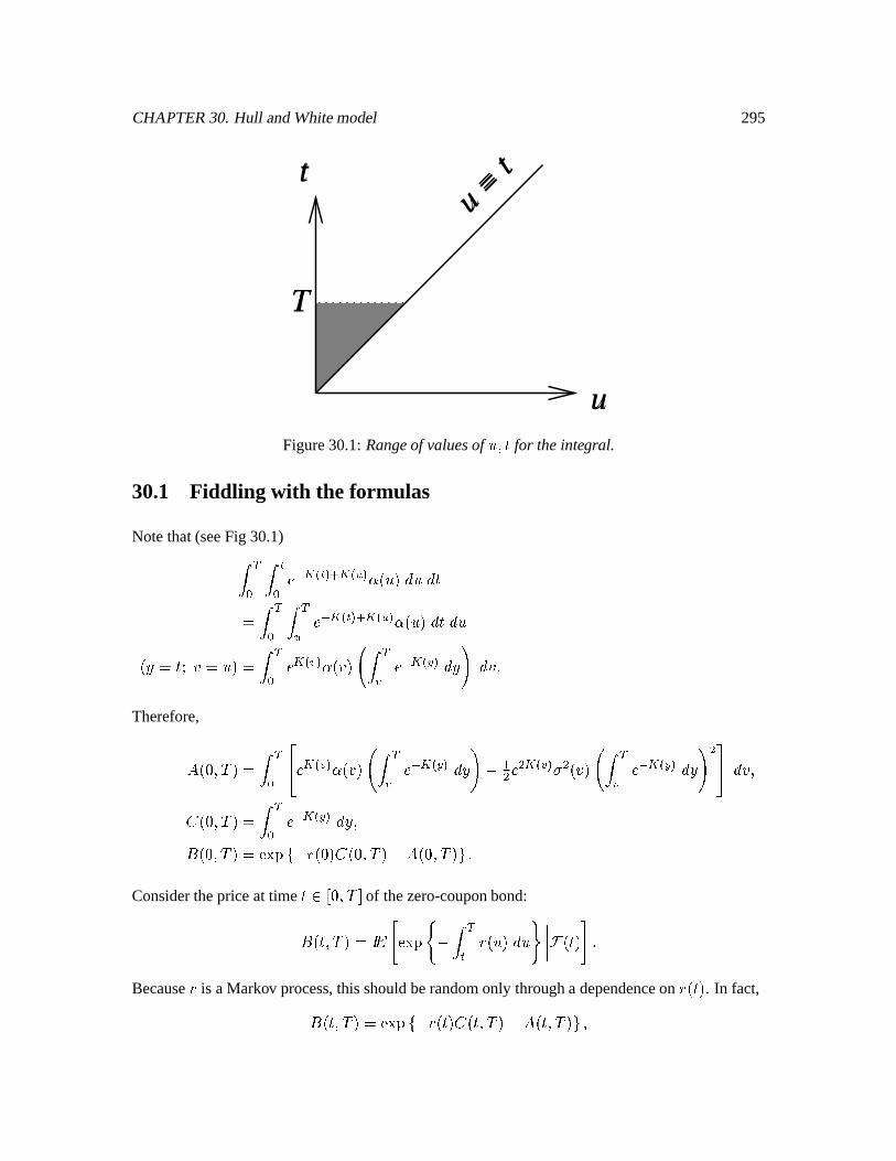
CHAPTER30. Hull andWhitemodel 295
u
tu
= t
T
Figure30.1:Rangeof valuesof ^ for theintegral.
30.1 Fiddling with the formulas
Notethat(seeFig 30.1)ÿ ß2 ÿ É2 ~ ¬ Ï ÉõÐ ¬ ÏV Ð ù0o!#p Æ Æ V ÿ ß2 ÿ ßV ~ ¬ Ï ÉÑÐ ¬ ÏoV Ð ù0o!p Æ Æ o!¦ Vë wn V p V ÿ ß2 ¬ Ï Ð ù0on¬p ~ ÿ ß ~ ¬ Ï ª Ð Æ ¦ Æ n fTherefore,aHoÃh ^ Û¯p V ÿ ß2 áä ¬ Ïo Ð ù0onp ~ ÿ ß ~ ¬ Ï ª Ð Æ ¦N q ¢\ \ ¬ Ï Ð [ \ on¬p ~ ÿ ß ~ ¬ Ï ª Ð Æ ¦ \ åè Æ n ^§ oÃh ^ Û¯p V ÿ ß2 ~ ¬ Ï ª Ð Æ ¦ ^Ê oh ^ Û¯p VëüSýíï q Z ohp § oh ^ ÛJp q ajoh ^ ÛJp fConsiderthepriceat time
¸ © h ^ Û of thezero-couponbond:Ê o ^ Û¯p Ve 65õüSýí þ qsÿ ßÉ Z o!#p Æ o p87 fBecause
Zis aMarkov process,thisshouldberandomonly througha dependenceon
Z o p . In fact,Ê o ^ Û¯p VëüSýíJ q Z o p § o ^ Û¯p q ajo ^ Û¯p ^
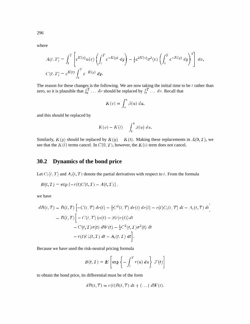
296
whereaHo ^ Û¯p V ÿ ßÉ áä ¬ Ïo Ð ù onp ~ ÿ ß ~ ¬ Ï ª Ð Æ ¦N q ¢\ \ ¬ Ïo Ð [ \ onp ~ ÿ ß ~ ¬ Ï ª Ð Æ ¦N \ åè Æ n ^§ o ^ Û¯p Ve ¬ Ï ÉÑÐ ÿ ßÉ ~ ¬ Ï ª Ð Æ ¦ fThereasonfor thesechangesis thefollowing. We arenow takingtheinitial time to be
ratherthan
zero,soit is plausiblethatT ß2 f8f8f Æ n shouldbereplacedby
T ßÉ f>f8f Æ n f Recallthatb on¬p V ÿ 2 ú o#p Æ ^andthisshouldbereplacedby b onp q«b o p V ÿ É ú o#p Æ fSimilarly,
b o!¦¬p shouldbereplacedbyb o!¦p qub o p . Making thesereplacementsin ajoh ^ Û¯p , we
seethattheb o p termscancel.In
§ oh ^ Û¯p , however, theb o p termdoesnot cancel.
30.2 Dynamicsof the bond price
Let
§ É o ^ Û¯p and a É o ^ ÛJp denotethepartialderivativeswith respectto
. FromtheformulaÊ o ^ ÛJp VëüSýíJ q Z o p § o ^ Û¯p q aHo ^ ÛJp ^
wehaveÆ¬Ê o ^ Û¯p V Ê o ^ Û¯p q § o ^ Û¯p Æ Z o p q ¢\ § \ o ^ ÛJp Æ Z o p Æ Z o p qÂZ o p § É o ^ Û¯p Æ q a É o ^ Û¯p Æ V Ê o ^ Û¯p ° q § o ^ Û¯pñoù o p q ú o p Z o pp Æ q § o ^ Û¯p [ o p Æ + o p q ¢\ § \ o ^ Û¯p [ \ o p Æ q«Z o p § É o ^ Û¯p Æ q a É o ^ Û¯p Æ ´ fBecausewehave usedtherisk-neutralpricing formulaÊ o ^ Û¯p Ve 65üSýíþ q ÿ ßÉ Z o!p Æ o p87to obtainthebondprice,its differentialmustbeof theformÆ¬Ê o ^ Û¯p V Z o p Ê o ^ Û¯p Æ c o f8f>f p Æ + o p f
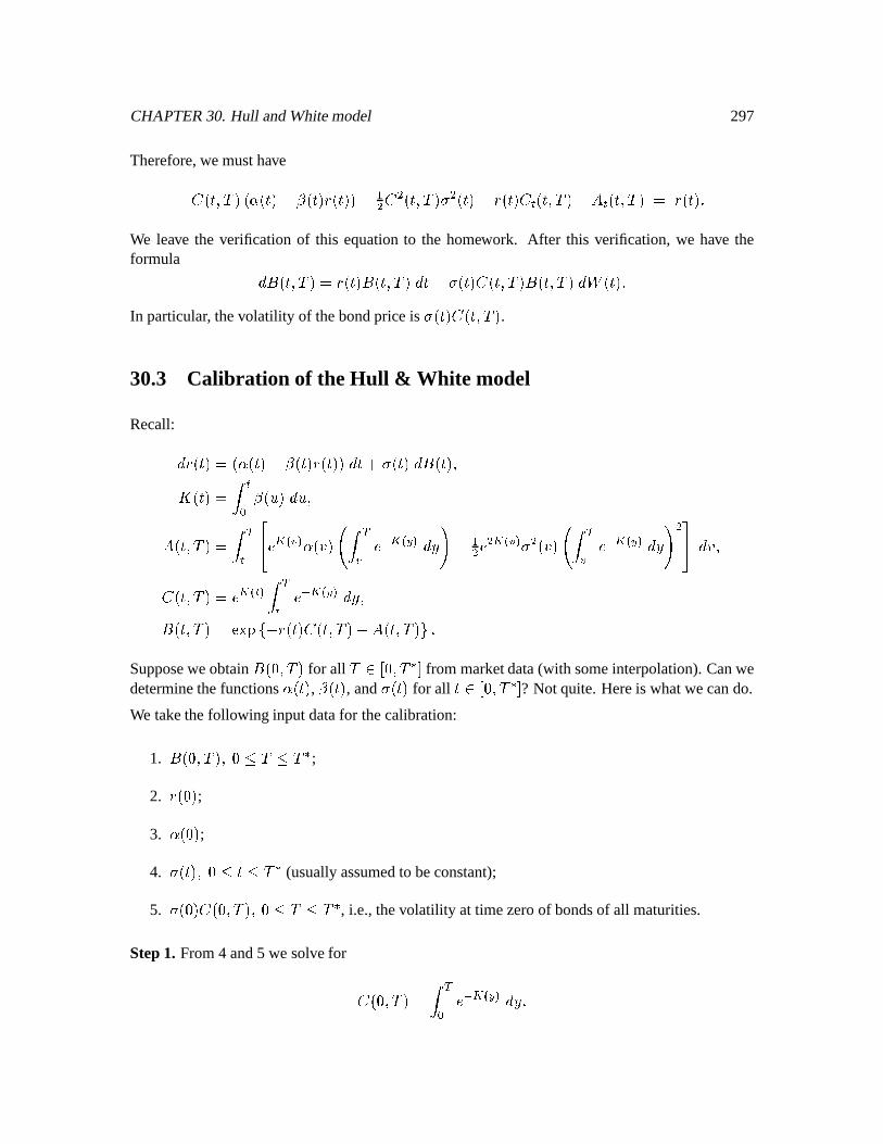
CHAPTER30. Hull andWhitemodel 297
Therefore,wemusthaveq § o ^ Û¯pNo*ù o p q ú o p Z o pp q ¢\ § \ o ^ Û¯p [ \ o p q«Z o p § É o ^ ÛJp q a É o ^ Û¯p V Z o p fWe leave the verificationof this equationto the homework. After this verification,we have theformula ÆÊ o ^ Û¯p V Z o p Ê o ^ Û¯p Æ q [ o p § o ^ Û¯p Ê o ^ ÛJp Æ + o p fIn particular, thevolatility of thebondpriceis [ o p § o ^ Û¯p .30.3 Calibration of the Hull & White model
Recall:Æ Z o p V où o p q ú o p Z o pp Æ cu[ o p Æ¬Ê o p ^b o p V ÿ É2 ú o!p Æ ^aHo ^ Û¯p V ÿ ßÉ áä ¬ Ïo Ð ù onp ~ ÿ ß ~ ¬ Ï ª Ð Æ ¦ q ¢\ \ ¬ Ïo Ð [ \ oÃn¬p ~ ÿ ß ~ ¬ Ï ª Ð Æ ¦ \ åè Æ n ^§ o ^ Û¯p Vø ¬ Ï ÉõÐ ÿ ßÉ ~ ¬ Ï ª Ð Æ ¦ ^Ê o ^ Û¯p V¨üSýíJ q Z o p § o ^ Û¯p q ajo ^ Û¯p fSupposeweobtain
Ê oh ^ Û¯p for all Û½¸ © h ^ Û ` from marketdata(with someinterpolation).Canwedeterminethefunctionsù0o p , ú o p , and [ o p for all
¸ © h ^ Û ` ? Not quite.Hereis whatwecando.
We takethefollowing inputdatafor thecalibration:
1.Ê oh ^ Û¯p ^ hÕiuÛeiuÛ ` ;
2.Z oÃhp ;
3. ù ohp ;4. [ o p ^ hji iuÛ ` (usuallyassumedto beconstant);
5. [ oÃhp § oÃh ^ Û¯p ^ hjiuÛÀiuÛ ` , i.e., thevolatility at timezeroof bondsof all maturities.
Step1. From4 and5 we solvefor § oh ^ Û¯p V ÿ ß2 ~ ¬ Ï ª Ð Æ ¦ f
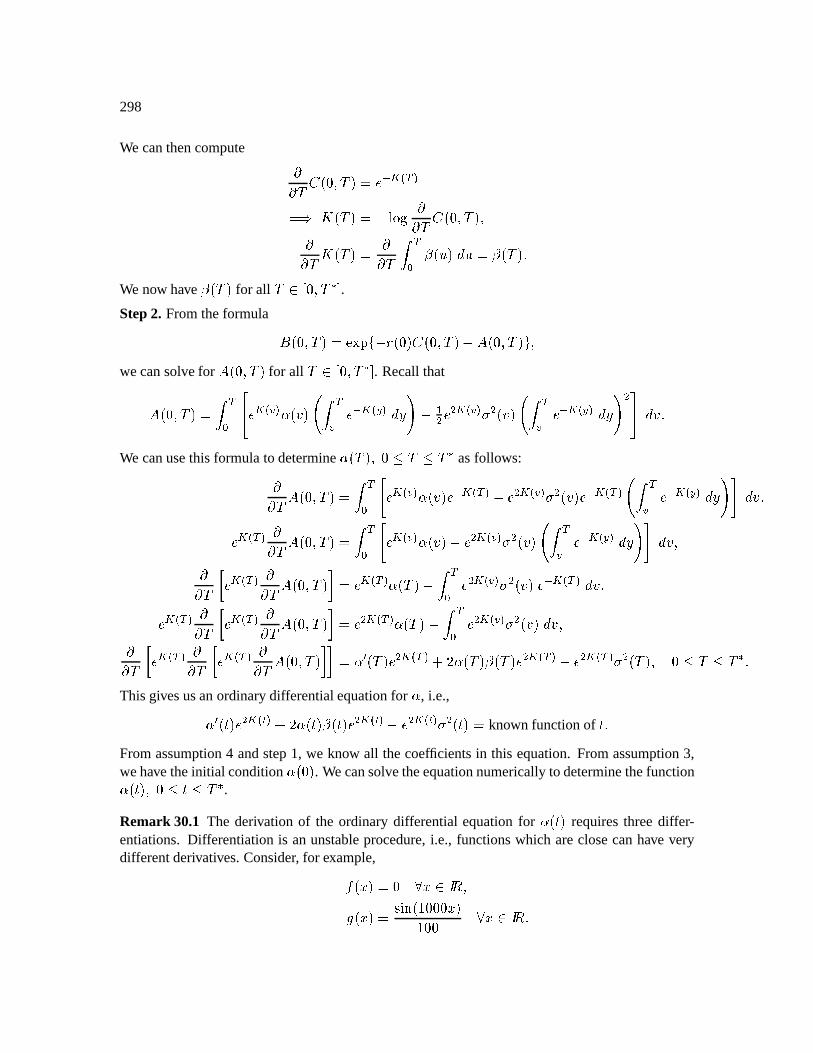
298
We canthencompute uu Û § oh ^ ÛJp Ve ~ ¬ Ï ß ÐVR¯ b oõÛ¯p V q Þ uu Û § oÃh ^ Û¯p ^uu Û b oõÛ¯p V uu Û ÿ ß2 ú o!p Æ V ú oõÛ¯p fWe now have ú oõÛJp for all Ûe¸ © h ^ Û ` .Step2. Fromtheformula Ê oh ^ Û¯p V¨üSýí q Z ohp § oh ^ Û¯p q aHoh ^ Û¯p ^wecansolvefor ajoh ^ ÛJp for all Ûe¸ © h ^ Û ` . Recallthatajoh ^ Û¯p V ÿ ß2 áä ¬ Ïo Ð ù0on¬p ~ ÿ ß ~ ¬ Ï ª Ð Æ ¦ q ¢\ \ ¬ Ïo Ð [ \ oÃn¬p ~ ÿ ß ~ ¬ Ï ª Ð Æ ¦ \ åè Æ n fWe canusethis formulato determineù oõÛJp ^ hjiuÛ½iuÛ ` asfollows:uu Û ajoh ^ Û¯p V ÿ ß2 5 ¬ Ï Ð ù0onp ~ ¬ Ï ß Ð q \ ¬ Ïo Ð [ \ oÃn¬p ~ ¬ Ï ß Ð ~ ÿ ß ~ ¬ Ï ª Ð Æ ¦7 Æ n ^ ¬ Ï ß Ð uu Û ajoh ^ Û¯p V ÿ ß2 5 ¬ Ï Ð2ù0onp q \ ¬ Ïo Ð [ \ oÃn¬p ~ ÿ ß ~ ¬ Ï ª Ð Æ ¦N°7 Æ n ^uu Û ° ¬ Ï ß Ð uu Û ajoh ^ Û¯p ´ Vø ¬ Ï ß Ðù oÇÛ¯p q ÿ ß2 \ ¬ Ï Ð [ \ onp ~ ¬ Ï ß Ð Æ n ^ ¬ Ï ß Ð uu Û ° ¬ Ï ß Ð uu Û ajoh ^ Û¯p ´ Vø \ ¬ Ï ß Ð ù oõÛJp q ÿ ß2 \ ¬ Ïo Ð [ \ onp Æ n ^uu Û ° ¬ Ï ß Ð uu Û ° ¬ Ï ß Ð uu Û aHoh ^ Û¯p ´S´ V ù ¡ oõÛ¯p \ ¬ Ï ß Ð c X ù oÇÛ¯p ú oõÛJp \ ¬ Ï ß Ð q \ ¬ Ï ß Ð [ \ oõÛ¯p ^ hÕiuÛeiuÛ ` fThisgivesusanordinarydifferentialequationfor ù , i.e.,ù ¡ o p \ ¬ Ï ÉÑÐ c X ù o p ú o p \ ¬ Ï ÉÑÐ q \ ¬ Ï ÉÑÐ [ \ o p V known functionof
fFromassumption4 andstep1, we know all thecoefficientsin this equation.Fromassumption3,wehave theinitial condition ù0ohp . Wecansolvetheequationnumericallyto determinethefunctionù0o p ^ hji iÈÛ ` .Remark 30.1 The derivation of the ordinarydifferentialequationfor ù o p requiresthreediffer-entiations.Dif ferentiationis anunstableprocedure,i.e., functionswhich areclosecanhave verydifferentderivatives.Consider, for example,t ok#p V h òks¸ ¹ ^ okp V êÍ o d hhhk#pd hh òks¸ ¹ f
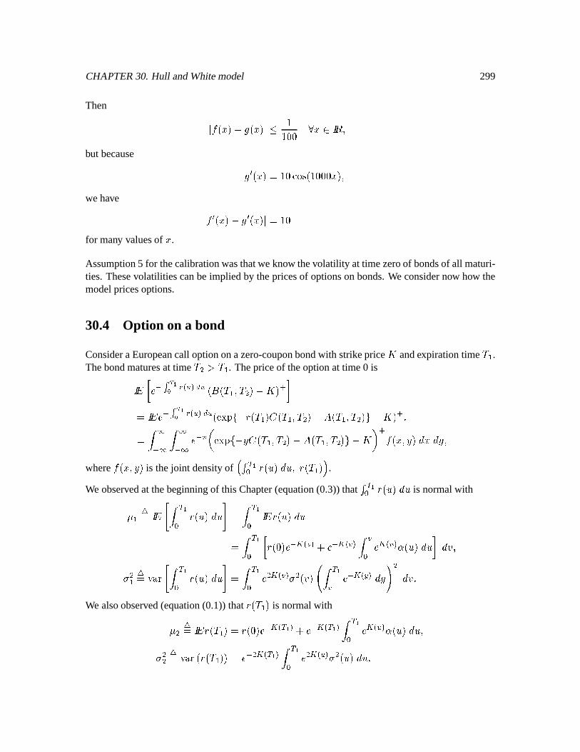
CHAPTER30. Hull andWhitemodel 299
Then t oÃk#p q ok#p i dd hh òks¸ ¹ ^but because ¡ ok#p V d h± ê o d hhhk#p ^wehave t ¡ok#p q ¡ÇoÃk#p V d hfor many valuesof k .
Assumption5 for thecalibrationwasthatweknow thevolatility at timezeroof bondsof all maturi-ties.Thesevolatilitiescanbeimplied by thepricesof optionsonbonds.We considernow how themodelpricesoptions.
30.4 Option on a bond
ConsideraEuropeancall optiononazero-couponbondwith strikepriceb
andexpirationtime Û ¢ .Thebondmaturesat time Û]\J¿uÛ ¢ . Thepriceof theoptionat time0 is ° ~ TR² "³ ÏoV ÐN´ V o Ê oõÛ ¢ ^ Û]\p q»b p ´Vø j ~ T² "³ ÏoV Ðz´ V o üSýí q Z oÇÛ ¢ p § oõÛ ¢ ^ Û\Íp q aHoÇÛ ¢ ^ Û]\,p qÂb p fV ÿ ~# ÿ ~# ~ ² üSýí q ¦ § oõÛ ¢ ^ Û]\p q aHoÇÛ ¢ ^ Û]\p q«b ³
t oÃk ^ ¦p Æ k Æ ¦ ^where
t ok ^ ¦¬p is thejoint densityofË T ß "2 Z o!#p Æ ^ Z oõÛ ¢ p Ì .
We observedat thebeginningof thisChapter(equation(0.3))thatT ß "2 Z o!#p Æ is normalwithZ ¢¶µVe S5 ÿ ß "2 Z o!#p Æ z7 V ÿ ß "2 Z o!p Æ V ÿ ß "2 ° Z ohp ~ ¬ Ï Ð c ~ ¬ Ï Ð ÿ 2 g¬ ÏoV Ð ù0o!p Æ ´ Æ n ^[ \ ¢ µV N®·5 ÿ ß "2 Z o!#p Æ z7 V ÿ ß "2 \ ¬ Ï Ð [ \ onp ~ ÿ ß " ~ ¬ Ï ª Ð Æ ¦ \ Æ n f
We alsoobserved(equation(0.1)) thatZ oõÛ ¢ p is normalwithZ \ µVe Z oõÛ ¢ p V Z ohp ~ ¬ Ï ß "ÇÐ c ~ ¬ Ï ß "RÐ ÿ ß "2 ¬ ÏV Ð%ù0o!#p Æ ^[ \\ µV N® o Z oõÛ ¢ pp Ve ~ \ ¬ Ï ß "ÃÐ ÿ ß "2 \ ¬ ÏV Ð [ \ o!#p Æ f
300
In fact,Ë T ß "2 Z o!#p Æ ^ Z oõÛ ¢ p%Ì is jointly normal,andthecovarianceis
i[ ¢ [ \ Ve 65 ÿ ß "2 o Z o#p q Z o!pp Æ f o Z oõÛ ¢ p q Z oõÛ ¢ pp87V ÿ ß "2 © o Z o!#p q Z o#pp0o Z oÇÛ ¢ p q Z oõÛ ¢ pp Æ V ÿ ß "2 i o! ^ Û ¢ p Æ ^wherei o! ^ Û ¢ p is definedin Equation0.2.
Theoptiononthebondhaspriceat timezeroof
ÿ ~# ÿ ~# ~ ² üSýí@ q ¦ § oõÛ ¢ ^ Û]\,p q aHoÇÛ ¢ ^ Û]\p q«b ³ dXN [ ¢ [ \¸ d q i\ üSýí þ q dX o d q i\ p 5 k \[ \ ¢ c X i k¦[ ¢ [ \ c ¦ \[ \\ 7 Æ k Æ ¦ f (4.1)
Thepriceof theoptionat time
¸ © h ^ Û ¢ is
° ~ T ² "¹ ÏoV д V o Ê oõÛ ¢ ^ Û]\,p q«b p o p ´Ve ° ~ T ² "¹ ÏoV д V o üSýí q Z oõÛ ¢ p § oÇÛ ¢ ^ Û]\p q ajoõÛ ¢ ^ Û\Íp q«b p o p ´ (4.2)
Becauseof the Markov property, this is randomonly througha dependenceonZ o p . To compute
this optionprice,we needthejoint distributionofË T ß "É Z o!p Æ ^ Z oÇÛ ¢ p Ì conditionedon
Z o p . This
CHAPTER30. Hull andWhitemodel 301
pairof randomvariableshasa jointly normalconditionaldistribution,andZ ¢ o p Ve S5 ÿ ß "É Z o!#p Æ o p87V ÿ ß "É ° Z o p ~ ¬ Ï Ð ¬ Ï ÉõÐ c ~ ¬ Ïo Ð ÿ É ¬ ÏV Ð ù o!p Æ ´ Æ n ^[ \ ¢ o p Ve áä ~ ÿ ß "É Z o#p Æ q Z ¢ o pL \ o p åèV ÿ ß "É \ ¬ Ï Ð [ \ onp ~ ÿ ß " ~ ¬ Ï ª Ð Æ ¦ \ Æ n ^Z \o p Ve ° Z oõÛ ¢ p Z o p ´V Z o p ~ ¬ Ï ß "RÐ ¬ Ï ÉÑÐ c ~ ¬ Ï ß "ÃÐ ÿ ß "É ¬ ÏV Ðù o#p Æ ^[ \\ o p Ve ° o Z oÇÛ ¢ p q Z \o pp \ o p ´Ve ~ \ ¬ Ï ß "RÐ ÿ ß "É \ ¬ ÏoV Ð [ \ o!p Æ ^i o p [ ¢ o p [ \o p Ve S5 ~ ÿ ß "É Z o!#p Æ q Z ¢ o pE o Z oõÛ ¢ p q Z \o ppy o p87V ÿ ß "É ~ ¬ ÏoV ÐÃ~ ¬ Ï ß "2Ð ÿ VÉ \ ¬ Ï Ð [ \ onp Æ n Æ fThe variancesandcovariancesarenot random. The meansarerandomthrougha dependenceonZ o p .Advantagesof theHull & Whitemodel:
1. Leadsto closed-formpricing formulas.
2. Allowscalibrationto fit initial yield curveexactly.
Short-comingsof theHull & White model:
1. One-factor, soonly allowsparallelshiftsof theyield curve, i.e.,Ê o ^ Û¯p VëüSýíJ q Z o p § o ^ Û¯p q aHo ^ Û¯p ^sobondpricesof all maturitiesareperfectlycorrelated.
2. Interestrateis normally distributed,andhencecantakenegative values.Consequently, thebondprice Ê o ^ Û¯p Ve S5õüSýíþ qsÿ ßÉ Z o#p Æ o pA7canexceed1.

302
Chapter 31
Cox-Ingersoll-Rossmodel
In theHull & Whitemodel,Z o p is aGaussianprocess.Since,for each
,Z o p isnormallydistributed,
thereisapositiveprobabilitythatZ o p0l3h . TheCox-Ingersoll-Rossmodelis thesimplestonewhich
avoidsnegative interestrates.
We begin with aÆ-dimensionalBrownian motion o + ¢ ^ + \ ^ f>f8f ^ + ´ p . Let ú ¿ h and [ ¿ h be
constants.For º V d ^ f8f8f ^ Æ , let Å ? oÃhp0¸ ¹ begivensothatÅ \¢ ohp c Å \\ ohp c f>f8f c Å \´ ohp h ^andlet Å ? bethesolutionto thestochasticdifferentialequationÆ Å ? o p V q ¢\ ú Å ? o p Æ c ¢\ [ Æ +? o p fÅ ? is calledtheOrstein-Uhlenbeck process.It alwayshasadrift towardtheorigin. ThesolutiontothisstochasticdifferentialequationisÅ ? o p Ve ~ ¢\ U É ° Å ? oÃhp c ¢\ [ ÿ É2 ¢\ U V Æ +¥? o!#p ´ fThissolutionis aGaussianprocesswith meanfunction ? o p Ve ~ ¢\ U É Å ? ohpandcovariancefunction i o! ^ p V d» [ \ ~ ¢\ U Ï ÉõÐ ÿ É2 U V Æ fDefine Z o p µV Å \¢ o p c Å \\ o p c f>f8f c Å \´ o p fIfÆ V d , we have
Z o p V Å \¢ o p andfor each
,
0 Z o p0¿3h V d , but (seeFig. 31.1) 01Thereareinfinitely many valuesof
¿3h for whichZ o p V h¼3 V d
303
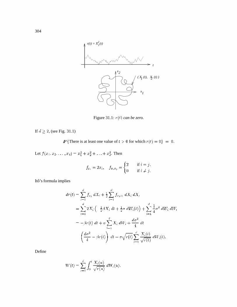
304
t
r(t) = X (t)
x
x
1
2( X (t), X (t) )1
12
2
Figure31.1:Z o p canbezero.
IfÆ X
, (seeFig. 31.1) 0 Thereis at leastonevalueof
¿3h for whichZ o p V h V h f
Let
t ok ¢ ^ k \ ^ f8f8f ^ k ´ p V k \ ¢ c k \\ c f8f8f c k \´ . Thent &½ V X k¾ ^ t &½¿ Vàþ Xif À V º ^h if À ºV º f
Ito’s formulaimpliesÆ Z o p V ´J ¾ K ¢t &½ Æ Å ¾ c ¢\ ´J ¾ K ¢
t &½&½ Æ Å ¾ Æ Å ¾V ´J ¾ K ¢ X Å ¾ Ë q ¢\ ú Å ¾ Æ c ¢\ [ Æ + ¾ o p Ì c ´J ¾ K ¢ d» [ \ Æ + ¾ Æ + ¾V q ú Z o p Æ c3[ ´J¾ K ¢ Å ¾ Æ + ¾ c Æ [ \» Æ V ~ Æ [ \» q ú Z o p Æ cu[Á Z o p ´J ¾ K ¢ Å ¾ o p¸ Z o p Æ + ¾ o p fDefine + o p V ´J ¾ K ¢ ÿ É2 Å ¾ o!p¸ Z o!#p Æ + ¾ o!#p f
CHAPTER31. Cox-Ingersoll-Rossmodel 305
Then
+is a martingale,Æ + V ´J ¾ K ¢ Å ¾ Z Æ + ¾ ^Æ + Æ + V ´J ¾ K ¢ Å \¾Z Æ ÖV Æ ^
so
+is a Brownianmotion.We haveÆ Z o p V ~ Æ [ \» q ú Z o p Æ cu[Á Z o p Æ + o p f
TheCox-Ingersoll-Ross(CIR)processis givenbyÆ Z o p V où q ú Z o pp Æ c3[ Á Z o p Æ + o p ^We define Æ V » ù[ \ ¿3h fIfÆ
happensto beaninteger, thenwe havetherepresentationZ o p V ´J ¾ K ¢ Å \¾ o p ^but wedonot require
Æto beaninteger. If
Æ l X (i.e., ù»l ¢\ [ \ ), then 0 Thereareinfinitely many valuesof
¿uh for whichZ o p V h V d f
This is nota goodparameterchoice.
IfÆ X
(i.e., ù ¢\ [ \ ), then 0 Thereis at leastonevalueof
¿3h for whichZ o p V h V h f
With the CIR process,onecan derive formulasunderthe assumptionthatÆ V Â [ ¢ is a positive
integer, andthey arestill correctevenwhenÆ
is not aninteger.
For example,hereis thedistributionofZ o p for fixed
¿3h . LetZ ohp h begiven.TakeÅ ¢ oÃhp V h ^ Å \ ohp V h ^ f8f>f ^ Å ´®~ ¢ oÃhp V h ^ Å ´ ohp V Á Z oÃhp f
For À V d ^ X ^ f>fSf ^ Æ q d , Å ¾ o p is normalwith meanzeroandvariancei o ^ p V [ \» ú o d q ~ U ÉRp f
306Å ´ o p is normalwith mean ´ o p Vø ~ ¢\ U É Á Z ohpandvariancei o ^ p . ThenZ o p V i o ^ p ´,~ ¢J ¾ K ¢ ~ Å ¾ o p¸ i o ^ p \y z |
Chi-squarewith ´~ ¢ KÃĤÅÆ,ÇÆ Çdegreesof
freedom
c Å \´ o py z |Normalsquaredandindependentof theother
term
(0.1)
ThusZ o p hasa non-central chi-squaredistribution.
31.1 Equilibrium distrib ution of vÈw'xAs
Ý¥t , ´ o pÍÝuh . We have Z o p V i o ^ p ´J¾ K ¢ ~ Å ¾ o p¸ i o ^ p \ fAs
Ýut , we have i o ^ p V [ ¢Â U , andso the limiting distribution ofZ o p is
[ ¢Â U timesa chi-square
withÆ V Â [ ¢ degreesof freedom.Thechi-squaredensitywith
 [ ¢ degreesof freedomist o¦¬p V dX \ [ ¢¡É Ë \ [ ¢ Ì ¦ ¢ ĤŠ[ ¢[ ¢ ~ ª \ fWe makethechangeof variable
Z V [ ¢Â U ¦ . Thelimiting densityforZ o p isÊ o Z p V » ú[@\ f dX \ [ ¢ É Ë \ [ ¢ Ì ² » ú[]\ Z ³ ¢
ĤŠ[ ¢[ ¢ ~ ¢Ë[ ¢ V ² X ú[]\ ³ ¢ Ä[ ¢ dÉ Ë \ [ ¢ Ì Z ¢ ĤŠ[ ¢[ ¢ ~ ¢Ë[ ¢ fWe computedthemeanandvarianceof
Z o p in Section15.7.
31.2 Kolmogorov forward equation
Considera Markov processgovernedby thestochasticdifferentialequationÆ ÅÈo p V m oõÅ3o pp Æ c¥[ oÇÅÈo pp Æ + o p f
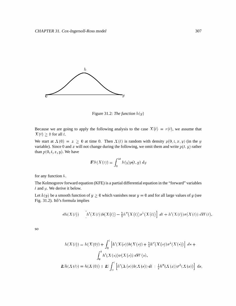
CHAPTER31. Cox-Ingersoll-Rossmodel 307
µé
h ¦Figure31.2:Thefunction éNo¦¬p
Becausewe aregoing to apply the following analysisto the caseÅ3o p V Z o p , we assumethatÅ3o p h for all
.
We startat ÅÈoÃhp V k h at time 0. Then Å3o p is randomwith density Ê oh ^ ^ k ^ ¦p (in the ¦variable).Since0 and k will notchangeduringthefollowing,weomit themandwrite Ê o ^ ¦p ratherthanÊ oh ^ ^ k ^ ¦¬p . We have éNoÇÅÈo pp V ÿ 2 éño!¦p Ê o ^ ¦p Æ ¦for any function é .
TheKolmogorov forwardequation(KFE) isapartialdifferentialequationin the“forward” variablesand ¦ . We derive it below.
Let éño!¦p beasmoothfunctionof ¦ h whichvanishesnear¦ V h andfor all largevaluesof ¦ (seeFig. 31.2).Ito’s formulaimpliesÆ éNoõÅ3o pp V é ¡ oõÅ3o pÍp m oõÅ o pp c¦¢\ é ¡¡ oõÅ3o pp [ \ oõÅ3o pp Æ c é ¡ oÇÅÈo pp [ oõÅ3o pÍp Æ + o p ^so
éNoõÅ3o pp V éNoõÅ3ohpÍp c ÿ É2 é¡RoõÅ3o!8pÍp m oõÅ3o8pp c ¢\ é<¡¡RoõÅ3o!8pp [ \ oõÅ3o!8pp Æ cÿ É2 é ¡ oõÅ3o!>pp [ oÇÅÈo8pp Æ + o!>p ^ éNoÇÅÈo pp V éNoõÅ3ohpÍp c ÿ É2 é ¡ oõÅ3o!8pp m oõÅ3oC>pp Æ c ¢\ é ¡¡ oõÅ3o!>pp [ \ oõÅ3o!8pp Æ ^
308
or equivalently,ÿ 2 éNo!¦p Ê o ^ ¦p Æ ¦ V éNoõÅ3ohpÍp c ÿ É2 ÿ 2 é ¡ o!¦¬p m o!¦¬p Ê o! ^ ¦¬p Æ ¦ Æ c¢\ ÿ É2 ÿ 2 é ¡¡ o!¦p [ \ o!¦p Ê o! ^ ¦p Æ ¦ Æ fDifferentiatewith respectto
to getÿ 2 éNo!¦p Ê É o ^ ¦p Æ ¦ V ÿ 2 é ¡ o!¦¬p m o!¦¬p Ê o ^ ¦¬p Æ ¦ c ¢\ ÿ 2 é ¡¡ o!¦p [ \ o!¦p Ê o ^ ¦p Æ ¦ f
Integrationby partsyieldsÿ 2 é ¡ o!¦p m o!¦p Ê o ^ ¦p Æ ¦ V éNo!¦p m o!¦p Ê o ^ ¦p ªK ª K 2y z, |K 2 q ÿ 2 éño!¦p uu ¦ o m o!¦p Ê o ^ ¦pp Æ ¦ ^ÿ 2 é ¡¡ o!¦¬p [ \ o!¦p Ê o ^ ¦p Æ ¦ V é ¡ o!¦p [ \ o!¦¬p Ê o ^ ¦¬p ªK ª K 2y z, |K 2 qsÿ 2 é ¡ o!¦¬p uu ¦ Ë [ \ o!¦p Ê o ^ ¦p Ì Æ ¦V q éNo!¦p uu ¦ Ë [ \ o!¦p Ê o ^ ¦p Ì ª
K ª K 2y z, |K 2 c ÿ 2 éNo¦¬p u \u ¦ \ Ë [ \ o!¦p Ê o ^ ¦p Ì Æ ¦ fTherefore,ÿ 2 éNo!¦p Ê É o ^ ¦p Æ ¦ V q ÿ 2 éNo!¦p uu ¦ o m o!¦p Ê o ^ ¦pp Æ ¦ c¦¢\ ÿ 2 éNo¦¬p u \u ¦ \ Ë [ \ o!¦p Ê o ^ ¦p Ì Æ ¦ ^or equivalently,ÿ 2 éño!¦¬p 5 Ê É o ^ ¦p c uu ¦ o m o!¦p Ê o ^ ¦pp q ¢\ u \u ¦ \ Ë [ \ o!¦p Ê o ^ ¦p%Ì 7 Æ ¦ V h fThis lastequationholdsfor every function é of theform in Figure31.2.It impliesthatÊ É o ^ ¦p c uu ¦ oo m o!¦p Ê o ^ ¦pp q ¢\ u \u ¦ \ Ë [ \ o¦¬p Ê o ^ ¦¬p Ì V h f (KFE)
If therewerea placewhere(KFE) did not hold, thenwe could take éNo!¦pj¿ h at thatandnearbypoints,but take é to bezeroelsewhere,andwe wouldobtainÿ 2 é 5 Ê É c uu ¦ o mEÊ p q ¢\ u \u ¦ \ o [ \ Ê pA7 Æ ¦¤ºV h f
CHAPTER31. Cox-Ingersoll-Rossmodel 309
If theprocessÅ3o p hasanequilibriumdensity, it will beÊ o!¦p V ÞÉ Ý Ê o ^ ¦¬p fIn orderfor this limit to exist, wemusthaveh V ÞÉ Ý Ê É o ^ ¦¬p fLetting
Ý3t in (KFE), weobtaintheequilibriumKolmogorov forwardequationuu ¦ o m o¦¬p Ê o!¦¬pÍp q ¢\ u \u ¦ \ Ë [ \ o!¦p Ê o¦¬p Ì V h fWhenanequilibriumdensityexists,it is theuniquesolutionto thisequationsatisfyingÊ o!¦p h òc¦ h ^ÿ 2 Ê o!¦p Æ ¦ V d f31.3 Cox-Ingersoll-Rossequilibrium density
We computedthis to beÊ o Z p V¨§ Z ¢ ĤŠ[ ¢[ ¢ ~ ¢Ë[ ¢ ^where §ÀV ² X ú[@\ ³ ¢ Ä[ ¢ dÉ Ë \ [ ¢ Ì fWe computeÊ ¡Ço Z p V X ù q [ \[@\ f Ê o Z pZ q X ú[\ Ê o Z pV X[ \ Z Ë ù q ¢\ [ \ q ú Z Ì Ê o Z p ^Ê ¡¡Ço Z p V q X[]\ Z \ Ë ù q ¢\ [ \ q ú Z Ì Ê o Z p c X[\ Z o q ú p Ê o Z p c X[]\ Z Ë ù q ¢\ [ \ q ú Z Ì Ê ¡Ão Z pV X[ \ Z ² q dZ où q ¢\ [ \ q ú Z p q ú c X[ \ Z où q ¢\ [ \ q ú Z p \ ³ Ê o Z pWe wantto verify theequilibriumKolmogorov forwardequationfor theCIR process:uu Z ooù q ú Z p Ê o Z pÍp q ¢\ u \u Z \ o [ \ Z Ê o Z pÍp V h f (EKFE)
310
Now uu Z o%où q ú Z p Ê o Z pÍp V q ú Ê o Z p c où q ú Z p Ê ¡ o Z p ^u \u Z \ o [ \ Z Ê o Z pÍp V uu Z o [ \ Ê o Z p c3[ \ Z Ê ¡Ço Z ppV X [ \ Ê ¡Ço Z p cu[ \ Z Ê ¡¡Ço Z p fTheLHS of (EKFE) becomesq ú Ê o Z p c où q ú Z p Ê ¡ o Z p q [ \ Ê ¡ o Z p q ¢\ [ \ Z Ê ¡ ¡ o Z pV Ê o Z p#° q ú c où q ú ZJq [ \ p X[@\ Z où q ¢\ [ \ q ú Z pc dZ où q ¢\ [ \ q ú Z p c ú q X[]\ Z où q ¢\ [ \ q ú Z p \ ´V Ê o Z p ° où q ¢\ [ \ q ú Z p X[\ Z où q ¢\ [ \ q ú Z pq ¢\ [ \ X[]\ Z où q ¢\ [ \ q ú Z pc dZ où q ¢\ [ \ q ú Z p q X[¾\ Z où q ¢\ [ \ q ú Z p \ ´V h ^asexpected.
31.4 Bond prices in the CIR model
TheinterestrateprocessZ o p is givenbyÆ Z o p V où q ú Z o pp Æ c3[4Á Z o p Æ + o p ^
whereZ ohp is given.ThebondpriceprocessisÊ o ^ Û¯p Ve 65õüSýí þ qsÿ ßÉ Z o!#p Æ o p87 f
Because üSýí 1 q ÿ É2 Z o#p Æ 3 Ê o ^ Û¯p Ve 5 üSýí þ q ÿ ß2 Z o!#p Æ o p 7 ^the tower propertyimplies that this is a martingale.The Markov propertyimplies that
Ê o ^ Û¯p israndomonly throughadependenceon
Z o p . Thus,thereis a functionÊ o Z ^ ^ Û¯p of thethreedummy
variablesZ ^ ^ Û suchthattheprocess
Ê o ^ Û¯p is thefunctionÊ o Z ^ ^ Û¯p evaluatedat
Z o p ^ ^ Û , i.e.,Ê o ^ ÛJp V Ê o Z o p ^ ^ Û¯p f
CHAPTER31. Cox-Ingersoll-Rossmodel 311
Because
üSýí d q T É2 Z o!p Æ f Ê o Z o p ^ ^ Û¯p is a martingale,its differentialhasnoÆ
term.We com-pute
Æ ² üSýí1 q ÿ É2 Z o!p Æ 43 Ê o Z o p ^ ^ ÛJp ³VëüSýí 1 qsÿ É2 Z o!#p Æ 3 ° q Z o p Ê o Z o p ^ ^ ÛJp Æ c Ê o Z o p ^ ^ Û¯p Æ Z o p c¢\ Ê % o Z o p ^ ^ Û¯p Æ Z o p Æ Z o p c Ê É o Z o p ^ ^ Û¯p Æ ´ fTheexpressionin
© f8f>f equalsV q Z ÊÀÆ c Ê où q ú Z p Æ c Ê [ Z Æ +c ¢\ Ê % [ \ Z Æ c Ê É Æ f
SettingtheÆ
termto zero,weobtainthepartialdifferentialequationq«Z Ê o Z ^ ^ ÛJp c Ê É o Z ^ ^ ÛJp c où q ú Z p Ê o Z ^ ^ Û¯p c ¢\ [ \ Z Ê 2 o Z ^ ^ ÛJp V h ^hji luÛ ^ Z h f (4.1)
Theterminalconditionis Ê o Z ^ Û ^ ÛJp V d ^ Z h fSurprisingly, this equationhasa closedform solution. Using theHull & White modelasa guide,we look for asolutionof theform Ê o Z ^ ^ Û¯p Ve ~ Ï É ß ÐÃ~ b Ï É ß Ð ^where
§ oõÛ ^ Û¯p V h ^ ajoõÛ ^ Û¯p V h . ThenwehaveÊ É V o q Z § É q a É p Ê ^Ê V q § Ê ^ Ê % Vë§ \ Ê ^andthepartialdifferentialequationbecomesh V q Z Ê c o q Z § É q a É p Ê q oÃù q ú Z p § Ê c ¢\ [ \ Z § \ ÊV Z Ê o q d q § É c ú § c¦¢\ [ \ § \ p q Ê o!a É c ù § pWe first solve theordinarydifferentialequationq d q § É o ^ ÛJp c ú § o ^ Û¯p c ¢\ [ \ § \ o ^ ÛJp V h< § oÇÛ ^ ÛJp V h ^andthenset ajo ^ Û¯p V ù ÿ ßÉ § o! ^ Û¯p Æ ^
312
so aHoÇÛ ^ ÛJp V h and a É o ^ Û¯p V q ù § o ^ Û¯p fIt is tediousbut straightforwardto checkthatthesolutionsaregivenby§ o ^ ÛJp V êÍÌ o U oõÛ q ppU ± êÌ o U oÇÛ q pÍp c ¢\ ú êÍÌ o U oõÛ q pp ^ajo ^ Û¯p V q X ù[]\ ÞoN áä U] ¢\ U Ï ß ~ÉÑÐU ± êÌ o U oõÛ q pp c£¢\ ú êÌ o U oÇÛ q pp åè ^where U¤V ¢\ Á ú \'c X []\ ^ êÌ V V q ~ VX ^ ± êÌ V V c ~ VX fThusin theCIR model,we have 65õüSýí þ q ÿ ßÉ Z o!#p Æ o p!7 V Ê o Z o p ^ ^ Û¯p ^where Ê o Z ^ ^ Û¯p VëüSýíJ q Z § o ^ Û¯p q ajo ^ Û¯p ^ hji luÛ ^ Z h ^and
§ o ^ Û¯p and ajo ^ Û¯p aregivenby theformulasabove. BecausethecoefficientsinÆ Z o p V où q ú Z o pp Æ cu[Á Z o p Æ + o pdo not dependon
, the function
Ê o Z ^ ^ Û¯p dependson
and Û only throughtheir difference VÛ q
. Similarly,
§ o ^ ÛJp and ajo ^ Û¯p arefunctionsof V Û q . We write
Ê o Z ^ p insteadofÊ o Z ^ ^ Û¯p , andwehaveÊ o Z ^ p VëüSýíJ q Z § o p q aHo p ^ h ^ Z h ^where § o p V êÌ o U pU ± êÌ o U p c£¢\ ú êÌ o U p ^ajo p V q X ù[]\ ÞoN áä U] ¢\ U U ± êÌ o U p c ¢\ ú êÌ o U p åè ^U¤V ¢\ Á ú \'c X []\ fWe have Ê o Z ohp ^ Û¯p Ve üSýíþ q ÿ ß2 Z o#p Æ fNow
Z o#pw¿3h for each , almostsurely, soÊ o Z ohp ^ Û¯p is strictly decreasingin Û . Moreover,Ê o Z oÃhp ^ hp V d ^
CHAPTER31. Cox-Ingersoll-Rossmodel 313Þß Ý Ê o Z ohp ^ Û¯p Vø «üSýí 1 qsÿ 2 Z o!p Æ 3 V h fBut also, Ê o Z ohp ^ Û¯p VëüSýíJ q Z ohp § oõÛ¯p q aHoÇÛ¯p ^so Z ohp § ohp c aHoÃhp V h ^Þß Ý © Z ohp § oõÛ¯p c aHoÇÛ¯p V t ^and Z oÃhp § oÇÛ¯p c aHoõÛJpis strictly inreasingin Û .
31.5 Option on a bond
Thevalueat time
of anoptiononabondin theCIR modelisn@o ^ Z o pp Ve S5ÑüSýíþ q ÿ ß "É Z o#p Æ o Ê oõÛ ¢ ^ Û]\p q«b p o p87 ^
whereÛ ¢ is theexpirationtimeof theoption, Û]\ is thematuritytimeof thebond,and hÕi iuÛ ¢ iÛ]\ . As usual,
üSýí·d q T É2 Z o!#p Æ f n@o ^ Z o pp is a martingale,andthis leadsto thepartialdifferentialequation q Z n c n É c où q ú Z pn c¦¢\ [ \ Z n % V h ^ hji luÛ ¢ ^ Z h f(where n V no ^ Z p .) TheterminalconditionisnoÇÛ ¢ ^ Z p V o Ê o Z ^ Û ¢ ^ Û \ p qÂb p ^ Z h fOtherEuropeanderivativesecuritiesonthebondarepricedusingthesamepartialdifferentialequa-tion with theterminalconditionappropriatefor theparticularsecurity.
31.6 Deterministic time changeof CIR model
Processtimescale: In this time scale,theinterestrateZ o p is givenby theconstantcoefficientCIR
equation Æ Z o p V où q ú Z o pp Æ c3[4Á Z o p Æ + o p fRealtimescale: In this timescale,theinterestrate ÍZ o Í p is givenby a time-dependentCIR equationÆ ÍZ o Í p V oÍù0o Í p q Íú o Í pzÍZ o Í pp Æ Í c Í[ o Í p Á ÍZ o Í p Æ Í+ o Í p f
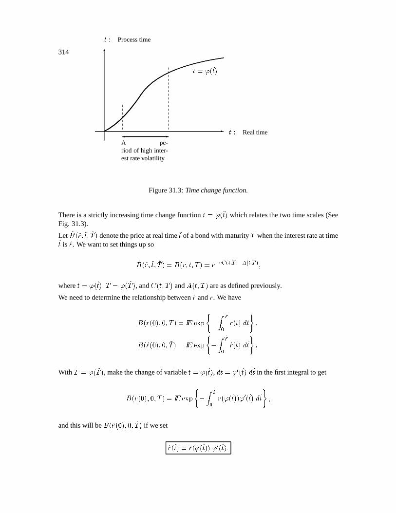
314
µ
¶
ÍÎ Realtime
ÎProcesstime 'VlÏ o Í p
.........
........
.
........
.
........
.
.........
.........
.........
.........
........
.
........
.
........
.
........
.
........
.
.........
.........
.........
.........
.........
.........
.........
.........
.........
.........
........
.
µÐA pe-riod of high inter-estratevolatility
Figure31.3:Timechangefunction.
Thereis a strictly increasingtime changefunction
VÑÏ o Í p which relatesthetwo time scales(SeeFig. 31.3).
Let ÍÊ o¤ÍZ ^ Í ^ ÍÛ p denotethepriceatrealtime Í of abondwith maturity ÍÛ whentheinterestrateat timeÍ is ÍZ . We wantto setthingsupsoÍÊ o¤ÍZ ^ Í ^ ÍÛ p V Ê o Z ^ ^ Û¯p Ve ~ Ï É! ß Ð~ b Ï É! ß Ð ^where
ÖVÒÏ o Í p ^ Û VlÏ o ÍÛJp , and
§ o ^ Û¯p and ajo ^ Û¯p areasdefinedpreviously.
We needto determinetherelationshipbetweenÍZ andZ. We haveÊ o Z ohp ^ h ^ ÛJp Vë »üSýí þ q ÿ ß2 Z o p Æ ^Ê o¤ÍZ ohp ^ h ^ ÍÛap Vë »üSýí þ qsÿÔÓß2 ÍZ o Í p Æ Í f
With Û VÒÏ o ÍÛ p , makethechangeof variable
ÖVÒÏ o Í p , Æ ÖVÒÏ ¡ o Í p Æ Í in thefirst integral to getÊ o Z ohp ^ h ^ ÛJp Vø «üSýíþ q ÿ Óß2 Z o Ï o Í pp Ï ¡Ño Í p Æ Í ^andthiswill be
Ê o¤ÍZ ohp ^ h ^ ÍÛap if wesetÍZ o Í p V Z o Ï o Í pp Ï ¡Ço Í p f
CHAPTER31. Cox-Ingersoll-Rossmodel 315
31.7 Calibration
ÍÊ o¤ÍZ o Í p ^ Í ^ ÍÛ p V Ê ~ ÍZ o Í pÏ ¡ o Í p ^ Ï o Í p ^ Ï o ÍÛ pEVëüSýíþ q ÍZ o Í p § o Ï o Í p ^ Ï o ÍÛ ppÏ ¡ o Í p q ajo Ï o Í p ^ Ï o ÍÛ0pp VëüSýíed q ÍZ o Í p ͧ o Í ^ ÍÛ p q Íajo Í ^ ÍÛ pgf ^where ͧ o Í ^ ÍÛ p V § o Ï o Í p ^ Ï o ÍÛ ppÏ ¡ o Í pÍajo Í ^ ÍÛ p V ajo Ï o Í p ^ Ï o ÍÛ0ppdo not dependon Í and ÍÛ only through ÍÛ q Í , since,in thereal time scale,themodelcoefficientsaretimedependent.
Supposewe know ÍZ ohp and ÍÊ o¤ÍZ ohp ^ h ^ ÍÛ p for all ÍÛe¸ © h ^ ÍÛ ` . We calibrateby writing theequationÍÊ o¤ÍZ ohp ^ h ^ ÍÛap VëüSýí·d q ÍZ ohp ͧ oh ^ ÍÛ p q ÍaHoh ^ ÍÛ pgf ^or equivalently, q Þ ÍÊ o¤ÍZ oÃhp ^ h ^ ÍÛ p V ÍZ ohpÏ ¡ ohp § o Ï ohp ^ Ï o ÍÛapp c ajo Ï ohp ^ Ï o ÍÛapÍp fTake ù ^ ú and [ sotheequilibriumdistributionof
Z o p seemsreasonable.Thesevaluesdeterminethe functions
§ ^ a . Take
Ï ¡ oÃhp V d (we justify this in the next section). For each ÍÛ , solve theequationfor
Ï o ÍÛ¯p : q Þ ÍÊ o¤ÍZ oÃhp ^ h ^ ÍÛap V ÍZ ohp § oh ^ Ï o ÍÛapp c ajoh ^ Ï o ÍÛ pÍp f (*)
The right-handsideof this equationis increasingin the
Ï o ÍÛ p variable,startingat 0 at time h andhaving limit t at t , i.e., ÍZ oÃhp § oÃh ^ hp c aHoÃh ^ hp V h ^ÞØß Ý © ÍZ oÃhp § oÃh ^ Û¯p c ajoh ^ Û¯p V t fSincehÕi q Þ ÍÊ o¤ÍZ ohp ^ h ^ ÍÛap0l¥t ^ (*) hasa uniquesolutionfor each ÍÛ . For ÍÛ V h , this solutionis
Ï ohp V h . If ÍÛ ¢ l ÍÛ]\ , thenq ÞoN ÍÊ o Z ohp ^ h ^ ÍÛ ¢ p0l q ÞoN ÍÊ o Z ohp ^ h ^ ÍÛ\%p ^so
Ï o ÍÛ ¢ p l Ï o ÍÛ]\p . Thus
Ïis astrictly increasingtime-change-functionwith theright properties.
316
31.8 Tracking down ÕÖ/w×x in the time changeof the CIR model
Resultfor generaltermstructuremodels:q uu Û Þ Ê oh ^ Û¯p ß K 2 V Z ohp fJustification: Ê oh ^ Û¯p Ve üSýíþ q ÿ ß2 Z o!#p Æ fq ÞoN Ê oh ^ Û¯p V q ÞoN0 üSýí þ q ÿ ß2 Z o#p Æ
q uu Û ÞoN Ê oh ^ Û¯p V ° Z oõÛ¯p ~ T ²³ ÏoV Ðz´ V ´ j ~ T ²³ ÏoV ÐN´ Vq uu Û ÞoN Ê oh ^ ÛJp ß K 2 V Z ohp fIn therealtimescaleassociatedwith thecalibrationof CIR by timechange,wewrite thebondpriceas ÍÊ o¤ÍZ oÃhp ^ h ^ ÍÛap ^therebyindicatingexplicitly theinitial interestrate.Theabove saysthatqØuu ÍÛ Þ ÍÊ o¤ÍZ ohp ^ h ^ ÍÛap Óß K 2 V ÍZ ohp fThe calibrationof CIR by time changerequiresthat we find a strictly increasingfunction
ÏwithÏ ohp V h suchthatq ÞoN ÍÊ o¤ÍZ ohp ^ h ^ ÍÛap V dÏ ¡ ohp ÍZ ohp § o Ï o ÍÛ0pp c ajo Ï o ÍÛ pp ^ ÍÛ h ^ (cal)
where ÍÊ o¤ÍZ ohp ^ h ^ ÍÛap , determinedby marketdata,is strictly increasingin ÍÛ , startsat1 when ÍÛ V h ,andgoesto zeroas ÍÛ¯Ý3t . Therefore,
q ÞoN ÍÊ o¤ÍZ ohp ^ h ^ ÍÛap is asshown in Fig. 31.4.
Considerthefunction ÍZ ohp § oõÛ¯p c aHoÇÛ¯p ^Here
§ oÇÛ¯p and aHoÇÛ¯p aregivenby§ oõÛ¯p V êÌ o U Û¯pU ± êÌ o U ÛJp c ¢\ ú êÌ o U Û¯p ^ajoõÛ¯p V q X ù[ \ ÞoN áä U] ¢\ U;ßU ± êÌ o U Û¯p c¦¢\ ú êÌ o U Û¯p åè ^UWV ¢\ Á ú \ c X [ \ f
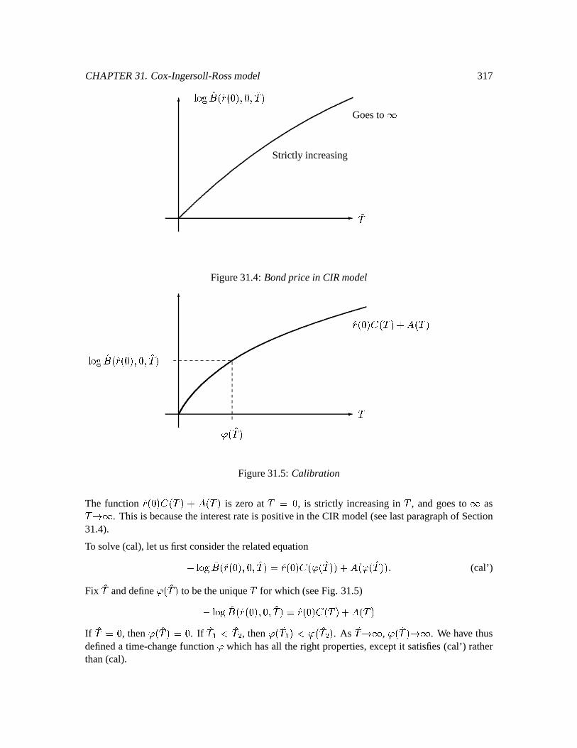
CHAPTER31. Cox-Ingersoll-Rossmodel 317
µ
¶Goesto t
Strictly increasing
ÍÛ
q ÞoN ÍÊ o¤ÍZ ohp ^ h ^ ÍÛap
Figure31.4:Bondprice in CIRmodel
µ
¶ ÍZ ohp § oõÛJp c ajoõÛ¯p
Û............................................................................................................ ......... ......... ......... ......... ......... ......... ......... ......... ......... .........
Ï o ÍÛ pq ÞoN ÍÊ o¤ÍZ ohp ^ h ^ ÍÛap
Figure31.5:Calibration
The function ÍZ ohp § oõÛ¯p c aHoõÛJp is zeroat Û V h , is strictly increasingin Û , andgoesto t asÛ¯Ýut . This is becausetheinterestrateis positivein theCIR model(seelastparagraphof Section31.4).
To solve(cal), let usfirst considertherelatedequationq ÞoN ÍÊ o¤ÍZ ohp ^ h ^ ÍÛap V ÍZ ohp § o Ï o ÍÛ pp c ajo Ï o ÍÛ pp f (cal’)
Fix ÍÛ anddefine
Ï o ÍÛ p to betheuniqueÛ for which(seeFig. 31.5)q ÞoN ÍÊ o¤ÍZ oÃhp ^ h ^ ÍÛap V ÍZ ohp § oõÛ¯p c aHoÇÛ¯pIf ÍÛ V h , then
Ï o ÍÛ p V h . If ÍÛ ¢ l ÍÛ \ , then
Ï o ÍÛ ¢ pl Ï o ÍÛ \ p . As ÍÛ¯Ý3t ,
Ï o ÍÛ¯pÝut . We have thusdefineda time-changefunction
Ïwhich hasall theright properties,exceptit satisfies(cal’) rather
than(cal).
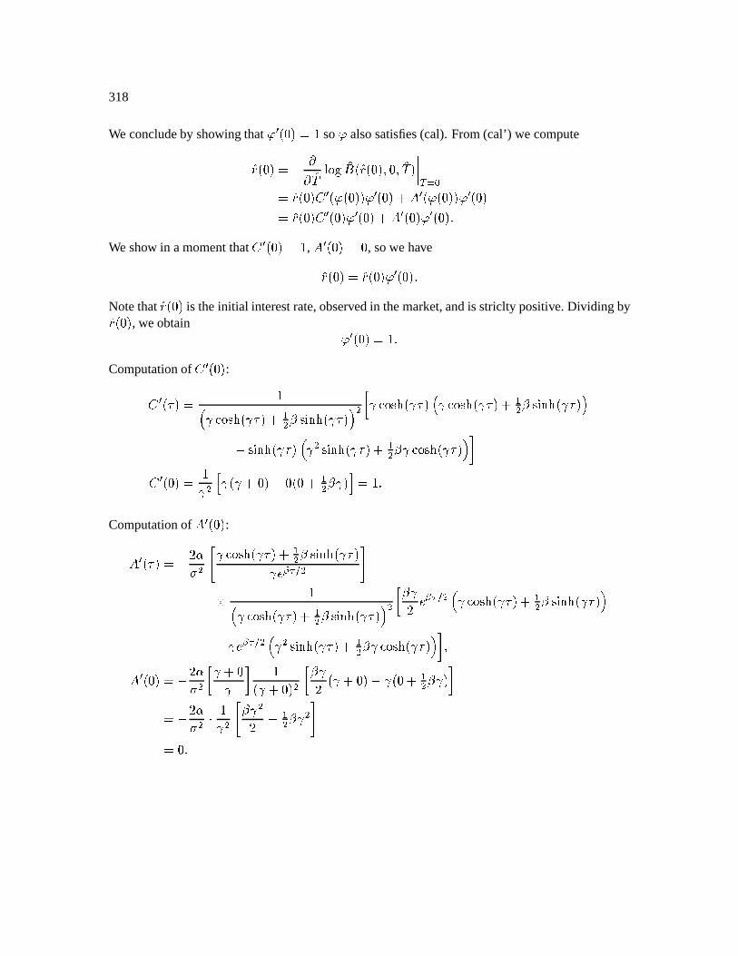
318
We concludeby showing that
Ï ¡ ohp V d so
Ïalsosatisfies(cal). From(cal’) we computeÍZ ohp V qØuu ÍÛ ÞoN ÍÊ o¤ÍZ ohp ^ h ^ ÍÛap Óß K 2V ÍZ ohp § ¡ o Ï ohpp Ï ¡ ohp c a ¡ o Ï ohpp Ï ¡ ohpV ÍZ ohp § ¡ÇoÃhp Ï ¡Ñohp c a ¡ohp Ï ¡ohp f
We show in amomentthat
§ ¡ ohp V d , a ¡ ohp V h , sowe haveÍZ oÃhp V ÍZ oÃhp Ï ¡ ohp fNotethat ÍZ ohp is theinitial interestrate,observedin themarket,andis striclty positive.Dividing byÍZ ohp , weobtain Ï ¡ ohp V d fComputationof
§ ¡ ohp :§ ¡Ro p V dË U ± êÌ o U p c¦¢\ ú êÌ o U p Ì \ ° U ± êÌ o U p Ë U ± êÌ o U p c ¢\ ú êÌ o U p Ìq êÌ o U p Ë U \ êÍÌ o U p c£¢\ ú U ± êÌ o U p Ì ´§ ¡ohp V dU \ U o U c hp q h#oh c£¢\ ú U p V d fComputationof a ¡ ohp :a ¡ o p V q X ù[]\ 5 U ± êÌ o U p c¦¢\ ú êÌ o U pU] U \ 7ö dË U ± êÌ o U p c ¢\ ú êÌ o U p Ì \ ° ú
UX U \ Ë U ± êÌ o U p c ¢\ ú êÌ o U p%Ìq U U \ Ë U \ êÍÌ o U p c£¢\ ú U ± êÌ o U p%Ì ´#^a ¡Rohp V q X ù[]\ ° U c hU ´ do U c hp \ °Íú UX o U c hp q U oh c ¢\ ú U p ´V q X ù[]\ dU \ 5 ú U \X q ¢\ ú U \ 7V h f
Chapter 32
A two-factor model (Duffie & Kan)
Let usdefine: Å ¢ o p V Interestrateat time
Å \ o p V Yield at time
onabondmaturingat time
cu 2Let Å ¢ oÃhp¿½h , Ū\ohp¿ h begiven,andlet Å ¢ o p and Ū\;o p begivenby thecoupledstochasticdifferentialequationsÆ Å ¢ o p V o k ¢¢ Å ¢ o p c k ¢ \ Å \ o p c#m ¢ p Æ cu[ ¢ Á ú ¢ Å ¢ o p c ú \ Å \ o p c ù Æ + ¢ o p ^ (SDE1)Æ Å \ o p V o k \ ¢ Å ¢ o p c k \Í\ Å \ o p c#m \ p Æ cu[ \ Á ú ¢ Å ¢ o p c ú \ Å \ o p c ù»o i Æ + ¢ o p c Á d q i \ Æ + \ o pp ^
(SDE2)
where
+ ¢ and
+ \ areindependentBrownianmotions.To simplify notation,we define
ÔWo p µV ú ¢ Å ¢ o p c ú \ Å \ o p c ù ^+ÚÙ o p µV i + ¢ o p c Á d q i \ + \ o p fThen
+ Ùis a Brownianmotionwith Æ + ¢ o p Æ + Ù o p V i Æ ^
and Æ Å ¢ Æ Å ¢ V [ \ ¢ Ô Æ ^ Æ Å \ Æ Åª\ V [ \\ Ô Æ ^ Æ Å ¢ Æ Åª\ V i[ ¢ [ \Ô Æ f319
320
32.1 Non-negativity of ÛÆ Ô V ú ¢ Æ Å ¢ c ú \ Æ Åª\V o ú ¢ k ¢¢ Å ¢ c ú ¢ k ¢ \,Ū\ c ú ¢ m ¢ p Æ c o ú \ k \ ¢ Å ¢ c ú \ k \\,Ū\ c ú \ m \,p Æ c Ôso ú ¢ [ ¢ Æ + ¢ c ú \ i[ \ Æ + ¢ c ú \ Á d q i\[ \ Æ + \,pV © o ú ¢ k ¢¢ c ú \ k \ ¢ p%Å ¢ c o ú ¢ k ¢ \ c ú \ k \\,p%Ū\ Æ c o ú ¢ m ¢ c ú \ m \p Æ c o ú \¢ [ \ ¢ c X ú ¢ ú \ i[ ¢ [ \ c ú \\ [ \\ p ¢\ Á ÔWo p Æ +  o p
where + Â o p V o ú ¢ [ ¢ c ú \ i[ \Sp + ¢ o p c ú \¸ d q i\[ \ + \o pÁ ú \¢ [ \ ¢ c X ú ¢ ú \ i[ ¢ [ \ c ú \\ [ \\is aBrownianmotion.We shallchoosetheparameterssothat:
Assumption1: For some
U, ú ¢ k ¢¢ c ú \ k \ ¢ V¨U ú ¢ ^ ú ¢ k ¢ \ c ú \ k \\ VëU ú \ f
Then Æ Ô V ©U ú ¢ Å ¢ c U ú \%Ū\ c ù U Æ c o ú ¢ m ¢ c ú \ m \ q ù U p Æ c o ú \¢ [ \ ¢ c X ú ¢ ú \ i[ ¢ [ \ c ú \\ [ \\ p ¢\ Ô Æ + ÂVëU Ô Æ c o ú ¢ m ¢ c ú \ m \ q ù U p Æ c o ú \¢ [ \ ¢ c X ú ¢ ú \ i[ ¢ [ \ c ú \\ [ \\ p ¢\ Ô Æ +  fFromourdiscussionof theCIR process,werecall that Ô will staystrictly positiveprovidedthat:
Assumption2: ÔWohp V ú ¢ Å ¢ ohp c ú \ÍŪ\ oÃhp c ù»¿3h ^and
Assumption3: ú ¢ m ¢ c ú \ m \ q U ù ¢\ o ú \¢ [ \ ¢ c X ú ¢ ú \ i[ ¢ [ \ c ú \\ [ \\ p fUnderAssumptions1,2,and3,Ôso p0¿3h ^ h±i l¥t ^ almostsurely,
and(SDE1)and(SDE2)makesense.Thesecanberewritten asÆ Å ¢ o p V o k ¢¢ Å ¢ o p c k ¢ \ÍŪ\o p c#m ¢ p Æ cu[ ¢ Á Ô o p Æ + ¢ o p ^ (SDE1’)Æ Å \ o p V o k \ ¢ Å ¢ o p c k \\ÍŪ\o p c#m \,p Æ cu[ \ Á Ô o p Æ + Ù o p f (SDE2’)
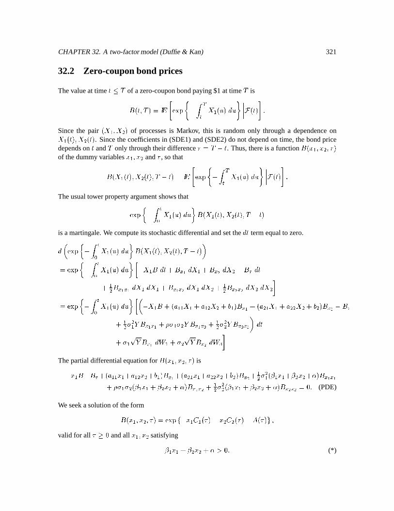
CHAPTER32. A two-factormodel(Duffie & Kan) 321
32.2 Zero-couponbond prices
Thevalueat time
iÈÛ of azero-couponbondpaying$1at time Û isÊ o ^ Û¯p Ve S5üSýíþ qsÿ ßÉ Å ¢ o!#p Æ o p87 fSincethe pair oÇÅ ¢ ^ Å \ p of processesis Markov, this is randomonly througha dependenceonÅ ¢ o p ^ Ū\;o p . Sincethecoefficientsin (SDE1)and(SDE2)do not dependon time, thebondpricedependson
and Û only throughtheir difference V Û q . Thus,thereis a function
Ê ok ¢ ^ k#\ ^ pof thedummyvariablesk ¢ ^ k \ and , sothatÊ oõÅ ¢ o p ^ Ū\8o p ^ Û q p Ve S5üSýí þ q ÿ ßÉ Å ¢ o!#p Æ o p87 fTheusualtowerpropertyargumentshowsthatüSýí 1 qsÿ É2 Å ¢ o!#p Æ 3 Ê oÇÅ ¢ o p ^ Ū\ o p ^ Û q pis amartingale.We computeits stochasticdifferentialandsetthe
Æ termequalto zero.Æ ² üSýí 1 qsÿ É2 Å ¢ o!#p Æ 3 Ê oõÅ ¢ o p ^ Å \ o p ^ Û q p ³VëüSýí 1 qsÿ É2 Å ¢ o!p Æ 3«° q Å ¢ Ê½Æ c Ê " Æ Å ¢ c Ê ¢ Æ Åª\ q Ê Æ c¦¢\ Ê " " Æ Å ¢ Æ Å ¢ c Ê " ¢ Æ Å ¢ Æ Å \ c¦¢\ Ê ¢ ¢ Æ Åª\ Æ Åª\ ´VëüSýí 1 qsÿ É2 Å ¢ o!p Æ 3«° ² q Å ¢ Ê c o k ¢¢ Å ¢ c k ¢ \Å \ c#m ¢ p Ê " c o k \ ¢ Å ¢ c k \Í\,Ū\ csm \p Ê ¢ q Ê c ¢\ [ \ ¢ Ô Ê " " cYi[ ¢ [ \ Ô Ê " ¢ c ¢\ [ \\ Ô Ê ¢ ¢ ³ Æ cu[ ¢ Ô Ê " Æ + ¢ cu[ \ Ô Ê ¢ Æ + Ù ´
ThepartialdifferentialequationforÊ ok ¢ ^ k#\ ^ p isq k ¢ Ê q Ê c o k ¢¢ k ¢ c k ¢ \Sk#\ cm ¢ p Ê " c o k \ ¢ k ¢ c k \\Sk\ cm \Sp Ê ¢ c»¢\ [ \ ¢ o ú ¢ k ¢ c ú \Sk#\ c ùNp Ê " "cYi[ ¢ [ \ o ú ¢ k ¢ c ú \ k \ c ùNp Ê " ¢ c ¢\ [ \\ o ú ¢ k ¢ c ú \ k \ c ùNp Ê ¢ ¢ V h f (PDE)
We seekasolutionof theformÊ oÃk ¢ ^ k\ ^ p VëüSýíJ q k ¢ § ¢ o p q k#\ § \o p q aHo p ^valid for all h andall k ¢ ^ k\ satisfyingú ¢ k ¢ c ú \Sk\ c ù¿¥h f (*)
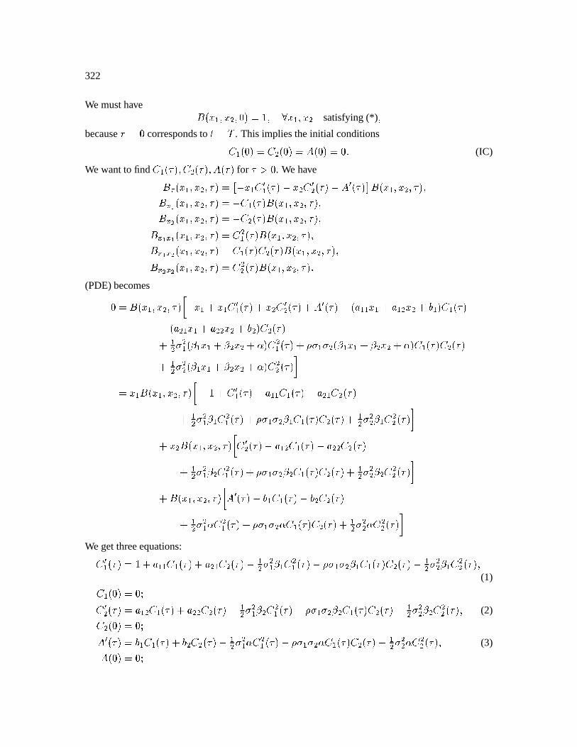
322
We musthave Ê ok ¢ ^ k \ ^ hp V d ^ òk ¢ ^ k \ satisfying(*) ^because V h correspondsto
'V Û . This impliestheinitial conditions§ ¢ ohp Vë§ \ ohp V aHoÃhp V h f (IC)
We wantto find
§ ¢ o p ^ § \ o p ^ ajo p for ¿3h . We haveÊ ok ¢ ^ k\ ^ p V î q k ¢ § ¡¢ o p q k\ § ¡\ o p q a ¡ o pPð Ê ok ¢ ^ k#\ ^ p ^Ê " ok ¢ ^ k\ ^ p V q § ¢ o p Ê oÃk ¢ ^ k\ ^ p ^Ê ¢ ok ¢ ^ k\ ^ p V q § \;o p Ê oÃk ¢ ^ k\ ^ p ^Ê " " ok ¢ ^ k\ ^ p Vë§ \¢ o p Ê ok ¢ ^ k#\ ^ p ^Ê " ¢ ok ¢ ^ k\ ^ p Vë§ ¢ o p § \8o p Ê ok ¢ ^ k\ ^ p ^Ê ¢ ¢ ok ¢ ^ k\ ^ p Vë§ \\ o p Ê ok ¢ ^ k#\ ^ p f(PDE)becomesh V Ê ok ¢ ^ k\ ^ p#° q k ¢ c k ¢ § ¡¢ o p c k\ § ¡\ o p c a ¡Ro p q o k ¢Í¢ k ¢ c k ¢ \Sk\ csm ¢ p § ¢ o pq o k \ ¢ k ¢ c k \\Sk\ csm \p § \ o pc£¢\ [ \ ¢ o ú ¢ k ¢ c ú \Sk#\ c ùñp § \¢ o p cYi[ ¢ [ \ o ú ¢ k ¢ c ú \k\ c ùNp § ¢ o p § \;o pc£¢\ [ \\ o ú ¢ k ¢ c ú \Sk#\ c ùñp § \\ o p ´V k ¢ Ê ok ¢ ^ k#\ ^ p ° q dac § ¡¢ o p q k ¢¢ § ¢ o p q k \ ¢ § \o pc ¢\ [ \ ¢ ú ¢ § \¢ o p cYi[ ¢ [ \ ú ¢ § ¢ o p § \;o p c ¢\ [ \\ ú ¢ § \\ o p ´c k \ Ê oÃk ¢ ^ k \ ^ p#° § ¡\ o p q k ¢ \ § ¢ o p q k \\ § \ o pc ¢\ [ \ ¢ ú \ § \¢ o p cYi[ ¢ [ \ ú \ § ¢ o p § \;o p c ¢\ [ \\ ú \ § \\ o p ´c Ê ok ¢ ^ k#\ ^ p ° a ¡ o p q m ¢ § ¢ o p q m \ § \;o pc ¢\ [ \ ¢ ù § \¢ o p cYi[ ¢ [ \ù § ¢ o p § \8o p c¦¢\ [ \\ ù § \\ o p ´We getthreeequations:§ ¡¢ o p V dac k ¢¢ § ¢ o p c k \ ¢ § \ o p q ¢\ [ \ ¢ ú ¢ § \¢ o p q i[ ¢ [ \ ú ¢ § ¢ o p § \>o p q ¢\ [ \\ ú ¢ § \\ o p ^
(1)§ ¢ ohp V h§ ¡\ o p Vlk ¢ \ § ¢ o p c k \\ § \;o p q ¢\ [ \ ¢ ú \ § \¢ o p q i[ ¢ [ \ ú \ § ¢ o p § \ o p q ¢\ [ \\ ú \ § \\ o p ^ (2)§ \ ohp V ha ¡ o p V m ¢ § ¢ o p c#m \ § \o p q ¢\ [ \ ¢ ù § \¢ o p q i[ ¢ [ \Sù § ¢ o p § \>o p q ¢\ [ \\ ù § \\ o p ^ (3)aHohp V h
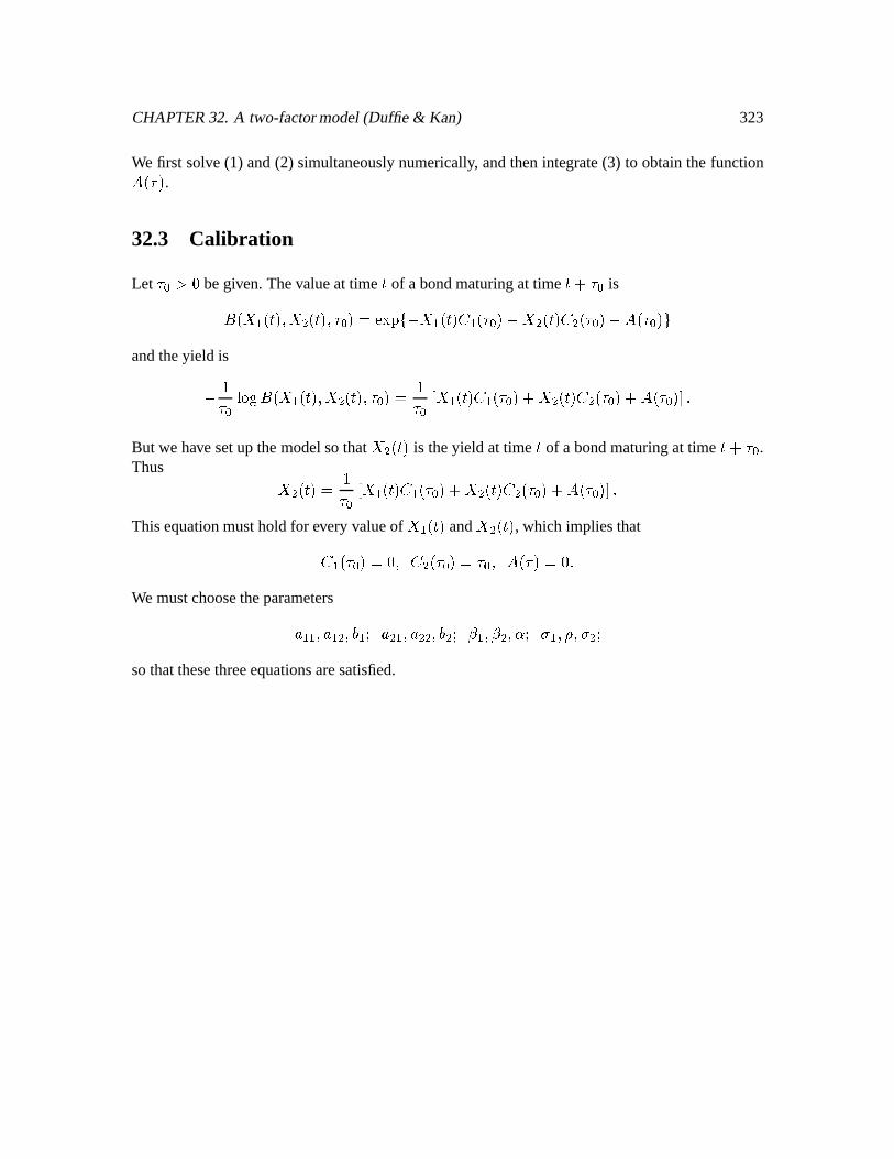
CHAPTER32. A two-factormodel(Duffie & Kan) 323
We first solve (1) and(2) simultaneouslynumerically, andthenintegrate(3) to obtainthe functionajo p .32.3 Calibration
Let 2 ¿3h begiven.Thevalueat time
of a bondmaturingat time
c¥ 2 isÊ oõÅ ¢ o p ^ Ū\>o p ^ 2 p V¨üSýí q Å ¢ o p § ¢ o 2 p q Ū\o p § \;o 2 p q ajo 2 p andtheyield isq d 2 ÞoN Ê oõÅ ¢ o p ^ Å \8o p ^ 2 p V d 2 © Å ¢ o p § ¢ o 2 p c Ū\ o p § \;o 2 p c ajo 2 p fBut we have setup themodelsothat Å \ o p is theyield at time
of a bondmaturingat time
c¥ 2 .Thus Ū\o p V d 2 © Å ¢ o p § ¢ o 2 p c Ū\ o p § \;o 2 p c ajo 2 p fThisequationmusthold for every valueof Å ¢ o p and Ū\o p , which impliesthat§ ¢ o 2 p V h ^ § \o 2 p V 2 ^ aHo p V h fWe mustchoosetheparametersk ¢¢ ^ k ¢ \ ^ m ¢ k \ ¢ ^ k \\ ^ m \> ú ¢ ^ ú \ ^ ùw [ ¢ ^ i ^ [ \;sothatthesethreeequationsaresatisfied.

324
Chapter 33
Changeof numeraire
Considera Brownian motion drivenmarketmodelwith time horizon Û ` . For now, we will haveoneasset,which we call a “stock” even thoughin applicationsit will usuallybe an interestratedependentclaim. Thepriceof thestockis modeledbyÆ o p V Z o p o p Æ cu[ o p o p Æ + o p ^ (0.1)
wherethe interestrateprocessZ o p andthe volatility process[ o p areadaptedto somefiltration o pS h i iëÛ ` . + is a Brownianmotionrelative to this filtration, but
o pS h i iëÛ ` maybelargerthanthefiltration generatedby
+.
This is not a geometricBrownianmotionmodel.We areparticularlyinterestedin thecasethattheinterestrateis stochastic,givenby a termstructuremodelwe havenot yet specified.
We shallwork only undertherisk-neutralmeasure,which is reflectedby thefact thatthemeanrateof returnfor thestockis
Z o p .We definetheaccumulationfactor
ú o p VëüSýí1 ÿ É2 Z o!p Æ 43 ^sothatthediscountedstockprice
ÎÏ ÉÑÐU Ï ÉÑÐ is amartingale.Indeed,Æ ² o pú o p ³ V o pú o p [ o p Æ + o p f
Thezero-couponbondpricesaregivenbyÊ o ^ Û¯p Ve S5üSýí þ qsÿ ßÉ Z o!#p Æ o p87Ve ° ú o pú oõÛ¯p o p ´ ^325
326
so Ê o ^ Û¯pú o p Ve ° dú oõÛ¯p o p ´is alsoa martingale(towerproperty).
The Û -forward price9 o ^ Û¯p of thestockis thepricesetat time
for deliveryof oneshareof stock
at time Û with paymentat time Û . Thevalueof theforwardcontractat time
is zero,soh Ve °ú o pú oõÛJp o
oõÛJp q=9 o ^ ÛJpp4 o p ´V ú o p ° oÇÛ¯pú oõÛ¯p 9 ´ qY9 o ^ Û¯p ° ú o pú oõÛ¯p o p ´V ú o p o pú o p qY9 o ^ Û¯p Ê o ^ ÛJpV o p qY9 o ^ Û¯p Ê o ^ ÛJp
Therefore, 9 o ^ Û¯p V o pÊ o ^ Û¯p fDefinition 33.1(Numeraire) Any assetin themodelwhosepriceis alwaysstrictly positivecanbetakenasthenumeraire.We thendenominateall otherassetsin unitsof thisnumeraire.
Example33.1(Money market asnumeraire) The money marketcould be the numeraire. At time Ü , thestockis worth ÝÞàßáâ ÞàßCá unitsof money marketandthe ã -maturitybondis worth äÞåß!æ çèáâ ÞàßCá unitsof money market.
Example33.2(Bond asnumeraire) The ã -maturitybondcouldbethenumeraire.At time Üé¥ã , thestockis worth êeëìÜíãïî unitsof ã -maturitybondandthe ã -maturitybondis worth1 unit.
We will saythata probabilitymeasure
0ñðis risk-neutral for thenumeraire if every assetprice,
dividedby , is a martingaleunder
0ð. Theoriginalprobabilitymeasure
0is risk-neutralfor the
numeraireú (Example33.1).
Theorem 0.71 Let bea numeraire, i.e., theprice processfor someassetwhoseprice is alwaysstrictly positive. Then
0ðdefinedby 0ñð oa¯p V duohp ÿ b uoõÛ ` pú oõÛ ` p Æ 0 ^ òca½¸ oõÛ ` p ^
is risk-neutral for .
CHAPTER33. Changeof numeraire 327
Note:
0and
0ñðareequivalent,i.e.,have thesameprobabilityzerosets,and 0 o!aJp V uohp ÿb ú oõÛ ` puoõÛ ` p Æ 0ð ^ òca½¸ oõÛ ` p f
Proof: Because is thepriceprocessfor someasset, ú is amartingaleunder
0. Therefore, 0ð o!- p V d oÃhp ÿ - uoõÛ ` pú oõÛ ` p Æ 0V d oÃhp f ° uoõÛ ` pú oõÛ ` p ´V d oÃhp uohpú ohpV d ^
andweseethat
0 ðis aprobabilitymeasure.
Let Ô be an assetprice. Under
0, Ô ú is a martingale.We mustshow that under
0ð, Ô is
a martingale.For this, we needto recallhow to combineconditionalexpectationswith changeofmeasure(Lemma1.54).If hji iuÛÀiÈÛ ` and Å is oÇÛ¯p -measurable,then òð ° Å o p ´ V oÃhp ú o puo p ° uoõÛ¯puohp ú oÇÛ¯p Å o p ´V ú o p o p ° uoõÛJpú oÇÛ¯p ÅG o p ´ fTherefore, óð ° ÔsoõÛJp oÇÛ¯p o p ´ V ú o p o p ° uoõÛJpú oÇÛ¯p ÔsoõÛ¯puoõÛJp o p ´V ú o p o p ÔWo pú o pV Ôso p o p ^which is themartingalepropertyfor Ô under
0ð.
33.1 Bond price asnumeraire
Fix ôrõ:ö!÷øhô¶ùLú andlet û©öüøhô¶ý bethenumeraire.Therisk-neutralmeasurefor thisnumeraireisþ ÿ ö ý û©ö!÷ø/ô ý û öô ø/ô¶ý öô¶ý þ ÿ û©ö!÷ø/ô ý öô¶ý þ ÿ õ öô¶ý
328
Becausethis bondis not definedafter time ô , we changethe measureonly “up to time ô ”, i.e.,using andonly for
õ¥öô¶ý .þ ÿis calledthe ô -forward measure. Denominatedin units of ô -maturity bond,the valueof the
stockis öüøhô¶ý öüAýû öüø/ô ý ø ÷ #ü!#ô"This is amartingaleunder
þ ÿ#, andsohasa differentialof theform öüø/ô¶ý%$'&¶öüø/ô ý öüøhô¶ý ( öüEýø ÷)#ü!#ô¶ø (1.1)
i.e., a differentialwithout a ü term. Theprocess* ( + ÷Ñü,Ñô.- is a Brownianmotionunderþ ÿ. Wemayassumewithout lossof generalitythat $&óöüøhô¶ý!/÷ .
We write
öüAý ratherthan
öüø/ô ý from now on.
33.2 Stockprice asnumeraire
Let öüAý be the numeraire. In termsof this numeraire,the stockprice is identically 1. The risk-neutralmeasureunderthisnumeraireisþ ÿ10 ö ý ö!÷Ný öô ù ý öô ù ý þ ÿ ø õ£öô ù ýDenominatedin sharesof stock,thevalueof the ô -maturitybondisû öüø/ô¶ý öüEý öüAý This is amartingaleunder
þ ÿ20, andsohasa differentialof theform
43 öüAý5 76ïöüøhô¶ý 3 öüAý5 8( 0 öüAýø (2.1)
where * ( 0 öüAý + ÷9Ôü ô¶ù:- is a Brownian motionunderþ ÿ10
. We may assumewithout lossofgeneralitythat 6ïöüø/ô¶ý/s÷ .Theorem 2.72 Thevolatility 6 öüø/ô ý in (2.1) is equalto the volatility $;&¶öüø/ô¶ý in (1.1). In otherwords,(2.1)canberewritten as
<3 öüEý 5 =$&óöüø/ô¶ý 3 öüEý 5 ( 0 öüEýø (2.1’)
CHAPTER33. Changeof numeraire 329
Proof: Let >ö@?ý :A ? , so >CBöD?ýFE GA ?'Hø!>CB BöD?ý=I A ?CJ . Then
3 öüAý 5 >ñö öüAý/ýK> B ö öüEý/ý öüAý#L H > B B ö öüAýhý öüEý öüAýFE H öüAý $&óöüøhô¶ý öüø/ô¶ý 8( öüAý#L J öüAý $ H& öüø/ô¶ý H öüø/ô¶ý ü öüEý M EN$;&¶öüøhô¶ý 8( öüEý#LO$ H& öüø/ô¶ý üQP=$&óöüøhô¶ý 3 öüEý 5SR E ( öüAýLO$;&¶öüøhô¶ý üúTUnder
þ ÿ# ø8E ( is aBrownianmotion.Underthismeasure, & VU hasvolatility $;&¶öüø/ô¶ý andmean
rateof return $H& öüø/ô ý . The changeof measurefromþ ÿ#
toþ ÿ20
makes & VU a martingale,i.e., itchangesthemeanreturnto zero,but thechangeof measuredoesnotaffect thevolatility. Therefore,6ïöüøhô¶ý in (2.1)mustbe $W&Èöüø/ô¶ý and ( 0 mustbe
( 0 öüAýXYE ( öüAý#L U $ & ö@Zñø/ô¶ý Z#
33.3 Merton option pricing formula
Thepriceat time zeroof a Europeancall is[ ö÷Ný þ \^] öô¶ý ö öô¶ý1E9_ýa`b þ \ ] öô¶ý öô ýc'd 0 DegfNh b E9_ þ \ ] öô ýicCd 0 DeCfjh b ö÷Ný d 0 DegfNh öô¶ý ö÷Ný öô ý þ ÿ E9_û ö!÷èø/ô¶ý d 0 @eCfNh û©ö!÷øhô¶ý öô ý þ ÿ ö÷Ný þ ÿ10 * öô¶ýkO_l-mE9_û ö÷ø/ô¶ý þ ÿ# * öô¶ýkO_l- ö÷Ný þ ÿ10 * öô¶ý!kO_l-mE9_û ö÷ø/ô¶ý þ ÿ# * öô¶ý!kO_l- ö÷Ný þ ÿ10.n öô¶ý)o _qp Er_û ö÷ø/ô¶ý þ ÿ# * öô¶ý!kO_l-8
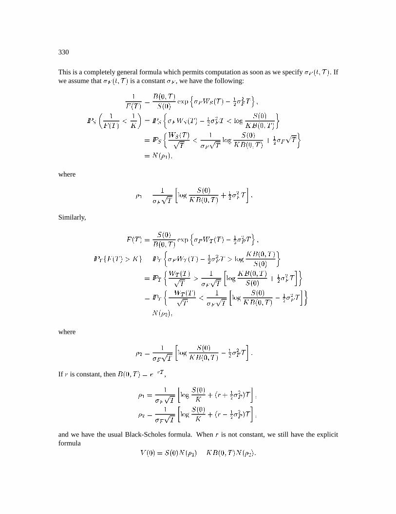
330
This is acompletelygeneralformulawhichpermitscomputationassoonaswespecify $;&¶öüø/ô¶ý . Ifweassumethat $ & öüø/ô ý is aconstant$ & , wehave thefollowing: öô¶ý û ö!÷èø/ô¶ý ö!÷Nýtsugvxw $;& ( 0 öô¶ý1E H $ H& ôzyeøþ ÿ10 3 öô¶ý o _ 5 þ ÿ10 n $& ( 0 öô¶ý1E H $ H& ô o|Vi~ ö!÷ý_û ö!÷øhô¶ý p þ ÿ 0zn ( 0 öô¶ý ô o $& ô Vi~ ö!÷Ný_û ö!÷øhô¶ý LH $ & ô p=#ö ýøwhere $ & ô ] ~ ö!÷Ný_û ö!÷èø/ô¶ý L H $ H& ô b Similarly, öô¶ý ö!÷Nýû ö!÷èø/ô¶ýsugv w $;& ( öô¶ý1E H $ H& ô y øþ ÿ# * öô¶ý!kO_l-. þ ÿ n $& ( öô ý2E H $ H& ôk Vi~ _û©ö!÷ø/ô ý ö!÷Ný p þ ÿ n ( öô¶ý ô k $;& ô ] Vi~ _û ö÷ø/ô¶ý ö!÷Ný L H $ H& ô!b p þ ÿ n E ( öô¶ý ô o $& ô ] Vi~ ö!÷Ný_û ö÷ø/ô¶ý E H $ H& ô b p=#ö H ýøwhere H $;& ô ] ~ ö!÷Ný_û ö!÷èø/ô¶ý EH $ H& ô!bNIf is constant,then û ö÷ø/ô¶ý%C , $& ô ] Vi~ ö!÷ý_ LröDXL^H $ H& ýEô!bóø H $& ô ] Vi~ ö!÷ý_ LröDNEFH $ H& ýEô!bóøandwe have the usualBlack-Scholesformula. When is not constant,we still have the explicitformula [ ö÷Ný2 ö!÷Ný ö ýE_¥û©ö!÷øhô¶ýa#ö H ý
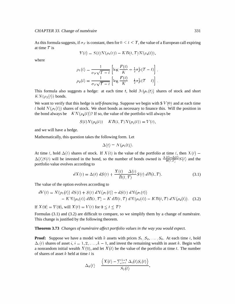
CHAPTER33. Changeof numeraire 331
As thisformulasuggests,if $& is constant,thenfor ÷#üô , thevalueof aEuropeancall expiringat time ô is [ öüEýX öüAý ö öüEý/ýE9_û öüø/ô¶ý ö H öüAý/ýøwhere öüAý $W& ôKE:ü ] Vi~ öüAý_ L^H $ H& öôOEüAýTb¶ø H öüAý $W& ôKE:ü ] Vi~ öüAý_ E H $ H& öôOEüAýTbmThis formula also suggestsa hedge: at eachtime ü , hold #ö öüAý/ý sharesof stock and short_#ö H öüAý/ý bonds.
We wantto verify thatthis hedgeis self-financing. Supposewebegin with $[ ö!÷ý andateachtimeü hold ö öüAý/ý sharesof stock. We shortbondsasnecessaryto financethis. Will thepositionin
thebondalwaysbe EN_#ö H öüEý/ý ? If so,thevalueof theportfolio will alwaysbe öüEýa#ö öüAý/ýE9_û©öüøhô¶ýa#ö H öüAýhý [ öüAýøandwewill have a hedge.
Mathematically, thisquestiontakesthefollowing form. Let öüAý=#ö öüEý/ýAt time ü , hold
öüAý sharesof stock. If öüAý is the valueof the portfolio at time ü , then öüAý!E öüEý öüAý will be investedin the bond,so the numberof bondsownedis VU VU UD öüEý andtheportfolio valueevolvesaccordingto öüEý2 öüAý 8 öüAýL öüAý1E öüAýû©öüøhô¶ý öüAý û öüø/ô¶ý (3.1)
Thevalueof theoptionevolvesaccordingto [ öüAý% ö öüAýhý 8 öüAýL öüAý ö öüAý/ý#L öüAý ö öüAý/ýE_ ö H öüAý/ý û öüø/ô¶ý1E_ û öüø/ô¶ý #ö H öüAýhýE9_û öüø/ô¶ý #ö H öüAý/ý (3.2)
If ö!÷Ný1 [ ö!÷ý , will öüEý [ öüAý for ÷)#üô ?
Formulas(3.1) and(3.2) aredifficult to compare,sowe simplify themby a changeof numeraire.Thischangeis justifiedby thefollowing theorem.
Theorem 3.73 Changesof numeraireaffectportfolio valuesin thewayyouwouldexpect.
Proof: Supposewe have a modelwith assetswith prices ø H øG:G¼ø # . At eachtime ü , hold) öüAý sharesof asset , 1 øIèøGG:ø)E , andinvesttheremainingwealthin asset . Begin witha nonrandominitial wealth ö!÷Ný , andlet öüAý bethevalueof theportfolio at time ü . Thenumberof sharesof asset heldat time ü is öüEýX öüEý2E9 ) öüAý öüEý¢¡ öüEý ø
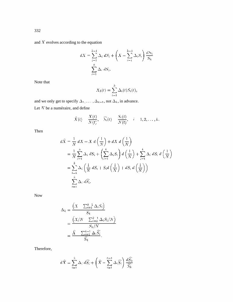
332
and evolvesaccordingto theequation
£ ¤ ¥ L§¦¨E ¤ ) ª© ¤ ) 8 Notethat öüAý ¤ öüAý öüEýøandweonly getto specify
øG:Gø , not , in advance.
Let bea numeraire,anddefine«#öüAý öüAý#öüEý ø¬ öüAý§ öüAý#öüAý ø # øIøG:øThen «® ¯L 3 5 L 3 5 ¤ ° ) L ¦ ¤ ¥ © <3 5 L ¤ ) 8 <3 5 ¤ ¥ 3 L 3 5 L 3 5X5 ¤ ¥ ¬ Now ± £E9 ° ) ¡#± A ²E9 ¥ A ³¡ A «¨E9 ° ¬ ¬ Therefore,
«® ¤ ¬ L ¦ «¨E ¤ ¬ © ¬ ¬
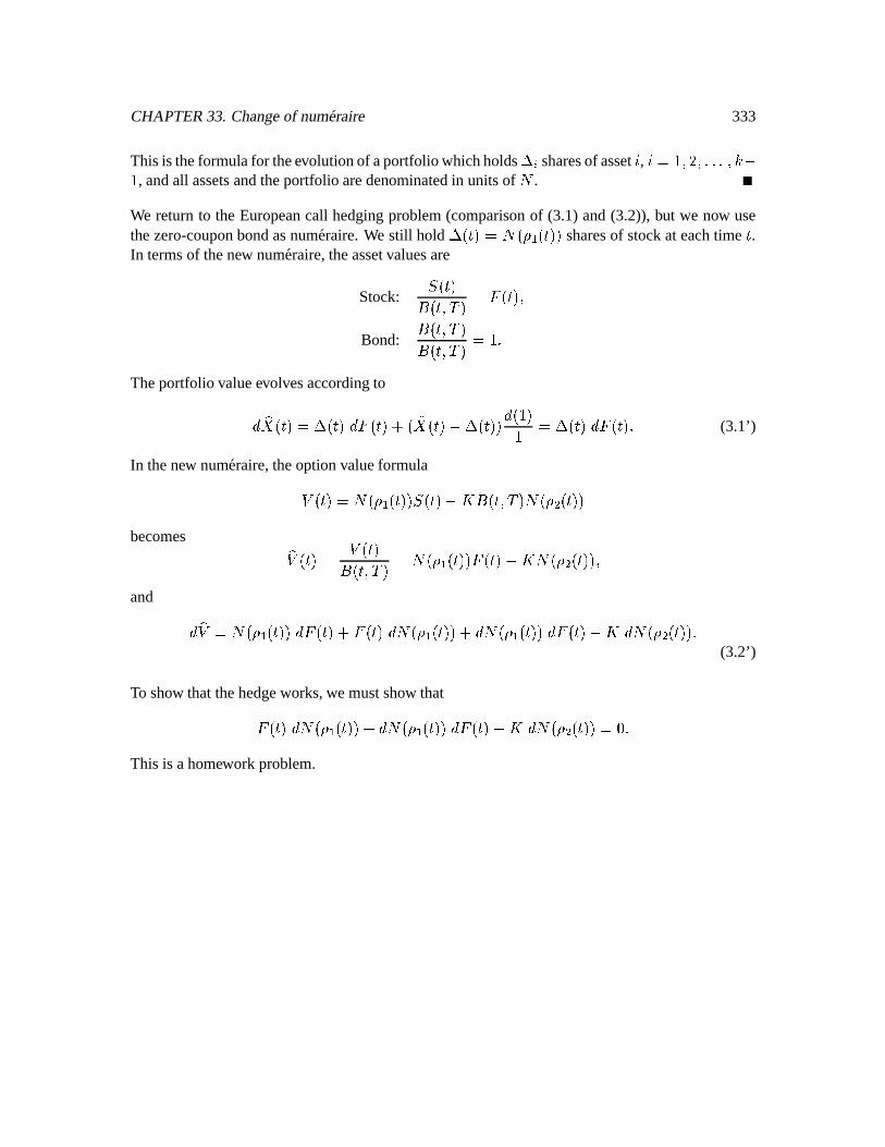
CHAPTER33. Changeof numeraire 333
Thisis theformulafor theevolutionof aportfoliowhichholds)
sharesof asset , # øIø:Gø2E, andall assetsandtheportfolio aredenominatedin unitsof .
We returnto the Europeancall hedgingproblem(comparisonof (3.1) and(3.2)), but we now usethezero-couponbondasnumeraire.We still hold
öüEýF#ö öüEý/ý sharesof stockat eachtime ü .In termsof thenew numeraire,theassetvaluesare
Stock: öüAýû©öüøhô¶ý öüEýøBond:
û©öüøhô¶ýû©öüøhô¶ý Theportfolio valueevolvesaccordingto « öüAý öüAý öüEý#Llö « öüAýE öüAý/ýi ö ý öüAý öüAý (3.1’)
In thenew numeraire,theoptionvalueformula[ öüEý=#ö öüAý/ý öüEý2E_û öüø/ô¶ýa#ö H öüEý/ýbecomes «[ öüAý [ öüAýû©öüøhô¶ý =#ö öüAýhý öüAý´Er_#ö H öüAý/ýgøand «[ =#ö öüEý/ý öüAý#L öüAý #ö öüEý/ýL #ö öüAý/ý öüEýE9_ #ö H öüEý/ý (3.2’)
To show thatthehedgeworks,wemustshow that öüAý #ö öüEý/ý#L ö öüAý/ý öüAý´Er_ #ö H öüEý/ýl÷CThis is ahomework problem.

334
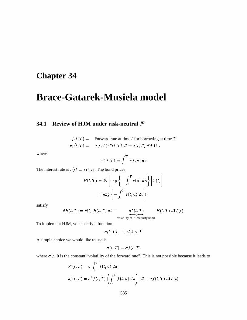
Chapter 34
Brace-Gatarek-Musielamodel
34.1 Review of HJM under risk-neutral µ·¶¸ öüøhô¶ý Forwardrateat time ü for borrowing at time ôz ¸ öüøhô¶ý $ïöüø/ô¶ý$ ù öüø/ô¶ý ü#L|$ïöüø/ô ý ( öüAýøwhere $ ù öüøhô¶ý2 U $öüøZ¼ý ZTheinterestrateis öüEýX ¸ öüø/üAý . Thebondpricesû öüø/ô ý þ \²¹ sugvzº E U |öDZý Z2»³¼¼¼¼ öüAý¾½ sugv¿º E U ¸ öüøZý Z2»satisfy û©öüøhô¶ý=öüEýû öüø/ô¶ý ü2E $ ù öüø/ô¶ýÀ Á Ã
volatility of
-maturitybond.
û öüø/ô¶ý ( öüAýTo implementHJM, youspecifya function$ïöüøhô¶ýø ÷ #ü!#ô"A simplechoicewewould like to useis$ öüø/ô ý=$ ¸ öüø/ô ýwhere$9k÷ is theconstant“volatility of theforwardrate”. This is notpossiblebecauseit leadsto$ ù öüø/ô¶ý1=$ U ¸ öüøZý Zø ¸ öüø/ô¶ý1=$ H ¸ öüø/ô¶ý ¦ U ¸ öüøZý Z © üLO$ ¸ öüøhô¶ý ( öüEýø
335
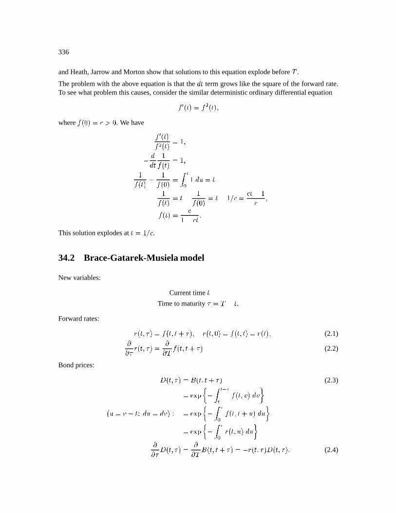
336
andHeath,Jarrow andMortonshow thatsolutionsto thisequationexplodebeforeô .
Theproblemwith theabove equationis that the ü termgrows like thesquareof theforwardrate.To seewhatproblemthiscauses,considerthesimilardeterministicordinarydifferentialequation¸ B öüEý ¸ H öüAýgøwhere ö!÷Ný=Ä.ks÷ . We have ¸ BöüAý¸ H öüEý øE ü ¸ öüEý øE ¸ öüAý L ¸ ö!÷Ný U ZGüE ¸ öüEý Gü1E ¸ ö!÷Ný Gü1E GA ÄX Äü1E Ä ø¸ öüEýX Ä E9Äü Thissolutionexplodesat üX GA Ä .34.2 Brace-Gatarek-Musielamodel
New variables:
Currenttime üTime to maturity Å [ôOEü
Forwardrates: öüøÅý2 ¸ öüø/üLOÅýø öüø÷Ný1 ¸ öüøhüAý=öüEýø (2.1)ÆÆ Å öüøÅý2 ÆÆ ô ¸ öüø/üL|Åý (2.2)
Bondprices: Ç öüøÅý1lû öüø/ü#L|Åý (2.3) suCv n E U `;ÈU ¸ öüøÉý É pöDZ =É¿E:ü + Z Ézý!Ê suCv n E È ¸ öüøhüLOZ¼ý Z p suCv n E È öüøZý Z pÆÆ Å Ç öüøÅý1 ÆÆ ô û öüø/ü#L|ÅýFENöüøÅý Ç öüøÅý (2.4)
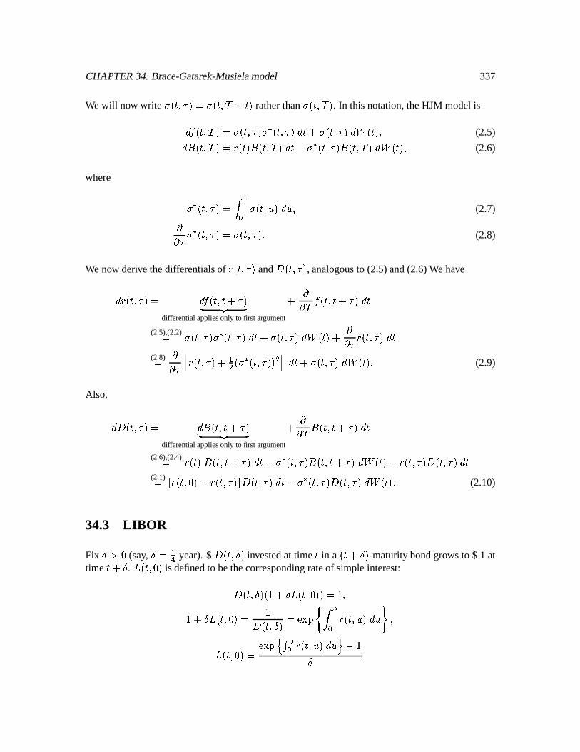
CHAPTER34. Brace-Gatarek-Musielamodel 337
We will now write $°öüøÅý2=$°öüøhôËE üAý ratherthan $ïöüøhô¶ý . In thisnotation,theHJM modelis ¸ öüøhô¶ý=$öüøÅýa$ ù öüøÅý ü#L|$ïöüøÅý 8( öüAýgø (2.5) û©öüøhô¶ý=öüAýhû öüø/ô¶ý ü2E9$ ù öüøÅýhû öüø/ô¶ý 8( öüEýø (2.6)
where $ ù öüøÅý È $öüøZ¼ý Zñø (2.7)ÆÆ Å $ ù öüøÅý=$öüøÅý (2.8)
We now derive thedifferentialsof öüøÅý and
Ç öüøÅý , analogousto (2.5)and(2.6)We have
öüøÅý1 ¸ öüøhüL|ÅýÀ ÁÂ Ãdifferentialappliesonly to first argument
L ÆÆ ô ¸ öüø/ü'LKÅý ü(2.5),(2.2) $ïöüøÅýa$ ù öüøÅý üL|$ïöüøÅý 8( öüAýL ÆÆ Å öüøÅý ü(2.8) ÆÆ ÅM öüøÅýL H ö@$ ù öüøÅý/ý H P üLK$ öüøÅý ( öüAý (2.9)
Also,
Ç öüøÅý1 û©öüøhüLKÅýÀ ÁÂ Ãdifferentialappliesonly to first argument
L ÆÆ ô û©öüøhüLKÅý ü(2.6),(2.4) öüAýû©öüøhü#L|Åý ü2E9$ ù öüøÅý/û öüø/üL|Åý ( öüAýE9öüøÅý Ç öüøÅý ü(2.1) R öüø÷NýEröüøÅý8ú Ç öüøÅý ü2Er$ ù öüøÅý Ç öüøÅý 8( öüAý (2.10)
34.3 LIBOR
Fix Ì kG÷ (say, Ìz Í year).$
Ç öüøÌý investedat time ü in a öüLOÌý -maturitybondgrows to $ 1 attime ü#L|Ì . ζöüø÷Ný is definedto bethecorrespondingrateof simpleinterest:Ç öüøÌý&ö L|Ìζöüø÷Nýhý2 ø LOÌÎ öüø÷Ný2 Ç öüøÌý sugv¿º ³Ï |öüøZ¼ý Z1»©øζöüø÷ý sugv wgÐ Ï |öüøZ¼ý Z y E Ì
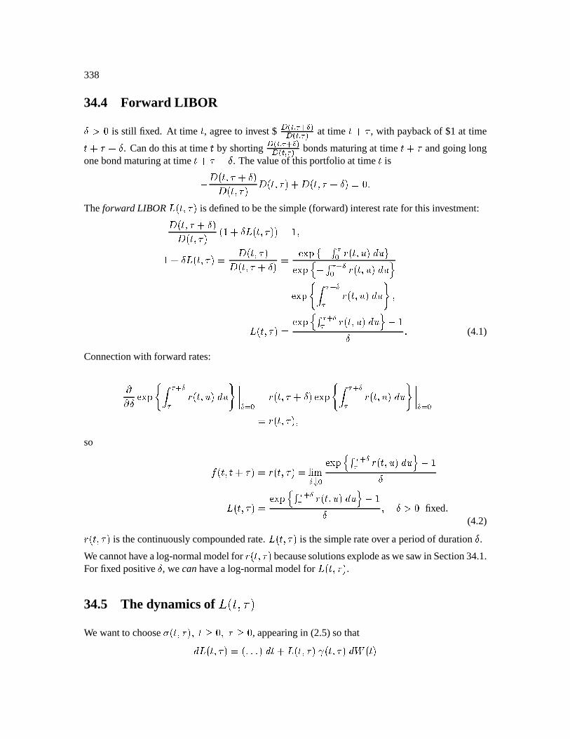
338
34.4 Forward LIBORÌ<kr÷ is still fixed. At time ü , agreeto invest$ Ñ VU@ ÈG`Ò Ñ VU@ È at time ü2LOÅ , with paybackof $1 at timeü#LOÅ¿LOÌ . Cando this at time ü by shorting Ñ VU@ ÈG`Ò Ñ VU@ È bondsmaturingat time ü#LOÅ andgoinglongonebondmaturingat time ü#L|Å.LKÌ . Thevalueof thisportfolio at time ü isE Ç öüøÅ.L|Ì,ýÇ öüøÅý Ç öüøÅýL Ç öüøÅ.L|Ì,ýÒ÷CTheforward LIBOR Î öüøÅý is definedto bethesimple(forward)interestratefor this investment:Ç öüøÅmLKÌýÇ öüøÅý ö L|ÌζöüøÅý/ý1 ø LKÌÓÎ öüøÅý2 Ç öüøÅýÇ öüøÅ"LOÌý suCv *8E Ð È öüøZý ZW-suCv w E Ð ÈG`Ò öüøZý Z y suCv º ÈG`ÒÈ |öüøZ¼ý Z » øζöüøÅý1 suCv w Ð ÈG`ÒÈ |öüøZ¼ý Z y E Ì (4.1)
Connectionwith forwardrates:ÆÆ Ì suCvzº ÈG`ÒÈ |öüøZ¼ý Z2»Ô¼¼¼¼ Ò =öüøÅmLKÌý suCv,º ÈG`ÒÈ |öüøZ¼ý Z1»³¼¼¼¼ Ò =öüøÅýøso ¸ öüø/üLKÅý=öüøÅý Õ ÖÒ¾× suCv.w Ð ÈG`ÒÈ öüøZ¼ý Z#y E ÌζöüøÅý1 suCv.w Ð ÈG`ÒÈ öüøZ¼ý Z#y E Ì ø Ì¿k÷ fixed
(4.2)öüøÅý is thecontinuouslycompoundedrate. ζöüøÅý is thesimplerateovera periodof durationÌ .Wecannothavealog-normalmodelfor öüøÅý becausesolutionsexplodeaswesaw in Section34.1.For fixedpositive Ì , wecanhave a log-normalmodelfor ζöüøÅý .34.5 The dynamicsof Ø9ÙÚ8ÛÜ!ÝWe wantto choose$ïöüøÅýø4ü/s÷øÅ/÷ , appearingin (2.5)sothat ζöüøÅý ö¢G:ý üLOÎ öüøÅý#6ïöüøÅý 8( öüAý
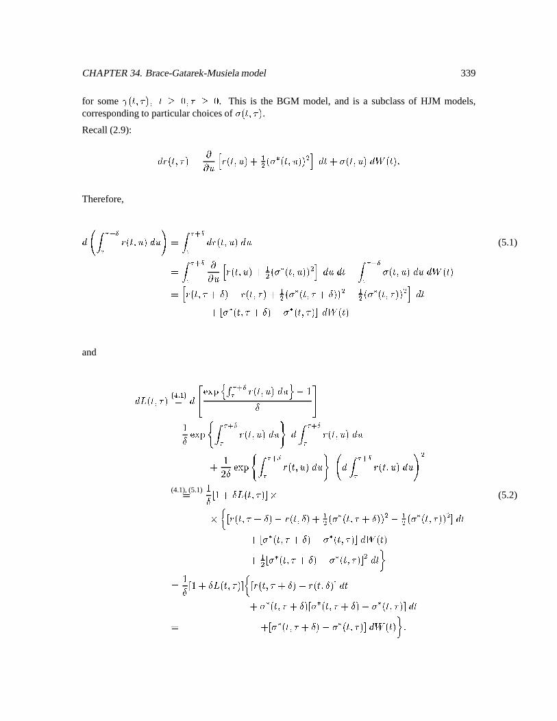
CHAPTER34. Brace-Gatarek-Musielamodel 339
for some 6 öüøÅýgø ü9/ ÷øÅY/ ÷ . This is the BGM model, and is a subclassof HJM models,correspondingto particularchoicesof $öüøÅý .Recall(2.9):
öüøÅý2 ÆÆ Z M |öüøZ¼ýL H ö@$ ù öüøZý/ý H P ü#L|$ïöüøZ¼ý ( öüAýTherefore,
¦ ÈG`ÒÈ |öüøZ¼ý Z © ÈG`ÒÈ |öüøZ¼ý Z (5.1) ÈG`ÒÈ ÆÆ Z M |öüøZ¼ýL^H ö@$ ù öüøZý/ý H P Z üL ÈG`ÒÈ $ïöüøZ¼ý Z ( öüAý M |öüøÅ"LOÌýE9öüøÅýL H ö@$ ù öüøÅ"LOÌý/ý H E H ö@$ ù öüøÅý/ý H P üL R $ ù öüøÅ.L|ÌýE9$ ù öüøÅý8ú ( öüAýand
Î öüøÅý ÍÞ lßà suCv.w Ð ÈG`ÒÈ öüøZ¼ý ZyáE Ì âã Ì"suCvzº ÈG`ÒÈ öüøZý Z2» ÈG`ÒÈ öüøZý ZL IÌ"sugvzº ÈG`ÒÈ |öüøZ¼ý Z2» ¦ ÈG`ÒÈ |öüøZ¼ý Z © H(4.1),(5.1) Ì R LKÌζöüøÅý8úä (5.2)ä n R öüøÅmLKÌý2EöüøÌ,ýLH öD$ ù öüøÅ"LOÌý/ý H EH öD$ ù öüøÅýhý H ú üL R $ ù öüøÅ.L|ÌýE9$ ù öüøÅý8ú ( öüAýL H R $ ù öüøÅ"LOÌý1Er$ ù öüøÅý8ú H ü p Ì R L|ÌζöüøÅýAú n R |öüøÅ.L|ÌýE9öüøÌý8ú üL|$ ù öüøÅ.L|Ìý R $ ù öüøÅ"LOÌý1Er$ ù öüøÅý8ú ü L R $ ù öüøÅmL|ÌýE$ ù öüøÅýAú ( öüAý p
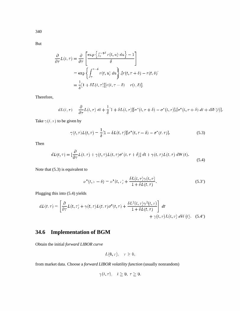
340
But ÆÆ Å Î öüøÅý ÆÆ Å ßà suCv w Ð ÈG`ÒÈ öüøZý Z y E Ì âã suCvzº ÈG`ÒÈ öüøZý Z1» R öüøÅ.L|ÌýE9öüøÌý8ú Ì R L|ÌζöüøÅýAú R öüøÅ"LOÌýE9öüøÌý8úTherefore,
Î öüøÅý ÆÆ Å Î öüøÅý üL Ì R L|ÌÎ öüøÅý8ú R $ ù öüøÅ.L|ÌýE9$ ù öüøÅýAú R $ ù öüøÅ"LOÌý üL ( öüAý8úQTake 6ïöüøÅý to begivenby6ïöüøÅýaÎ öüøÅý# Ì R LKÌζöüøÅý8ú R $ ù öüøÅmLKÌ,ý´E9$ ù öüøÅýAúD (5.3)
Then ζöüøÅý1 R ÆÆ Å Î¶öüøÅýL|6ïöüøÅýaÎ öüøÅýa$ ù öüøÅ"LOÌý8ú üL6ïöüøÅýaÎ öüøÅý ( öüEý(5.4)
Notethat(5.3) is equivalentto$ ù öüøÅ.L|ÌýX%$ ù öüøÅýL ÌζöüøÅýå6 öüøÅý L|ÌÓÎ öüøÅý (5.3’)
Pluggingthis into (5.4)yields
Î öüøÅý2 ¹ ÆÆ Å Î¶öüøÅýL6ïöüøÅýaÎ öüøÅýa$ ù öüøÅýL ÌÓÎ H öüøÅýå6 H öüøÅý L|ÌÓÎ öüøÅý ½ üL6ïöüøÅýaζöüøÅý 8( öüAý (5.4’)
34.6 Implementation of BGM
Obtaintheinitial forward LIBORcurve ζö÷øÅýøæÅ/÷øfrom marketdata.Choosea forward LIBORvolatility function(usuallynonrandom)6 öüøÅýgø ü!/÷øÅ/÷
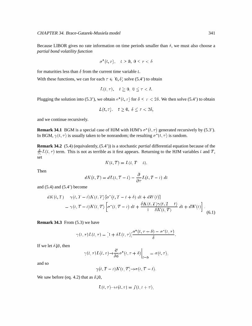
CHAPTER34. Brace-Gatarek-Musielamodel 341
BecauseLIBOR givesno rateinformationon time periodssmallerthan Ì , we mustalsochooseapartial bondvolatility function $ ù öüøÅýgø ü!/÷øï÷)KÅ o Ìfor maturitieslessthan Ì from thecurrenttimevariableü .With thesefunctions,wecanfor eachÅ õ R ÷øÌý solve(5.4’) to obtainÎ öüøÅýø ü!/÷øï÷)OÅ o ÌGPluggingthesolutioninto (5.3’), we obtain $ ù öüøÅý for ÌzKÅ o IiÌ . We thensolve(5.4’) to obtainζöüøÅýgø ü/÷èøXÌzKÅ o Ii̤øandwecontinuerecursively.
Remark 34.1 BGM is a specialcaseof HJM with HJM’s $ñùNöüøÅý generatedrecursively by (5.3’).In BGM, 6ïöüøÅý is usuallytakento benonrandom;theresulting$ ù öüøÅý is random.
Remark 34.2 (5.4)(equivalently, (5.4’)) is a stochasticpartial differentialequationbecauseof theÏÏ È Î¶öüøÅý term. This is not asterribleasit first appears.Returningto theHJM variablesü and ô ,set _#öüø/ô¶ý1=Î öüøhôOEüAýThen _ öüø/ô ý2 ζöüø/ô|EüEýE ÆÆ Å Î¶öüø/ô|EüEý üand(5.4)and(5.4’) become _#öüøhô¶ý176ïöüøhôrEüAý_ öüø/ô ý R $ ù öüøhôËEü#L|Ìý üL ( öüAý8ú76ïöüøhôrEüAý_ öüø/ô ý ] $ ù öüø/ô|E:üEý ü#L Ì_#öüøhô¶ý¢6ïöüø/ô9EüAý LKÌÓ_#öüø/ô¶ý üL ( öüAý b
(6.1)
Remark 34.3 From(5.3)wehave6ïöüøÅýaζöüøÅý R LOÌζöüøÅýAú $ùNöüøÅ"LOÌý1Er$RùNöüøÅýÌ If we let Ì × ÷ , then 6 öüøÅýζöüøÅýaç ÆÆ Ì $ ù öüøÅ"LOÌý¼¼¼¼ Ò %$ïöüøÅýøandso 6 öüø/ôE:üEýa_#öüøhô¶ýaç$ïöüøhô|EüAýWe saw before(eq.4.2)thatas Ì × ÷ ,ζöüøÅýaç|öüøÅý1 ¸ öüøhüL|Åýø
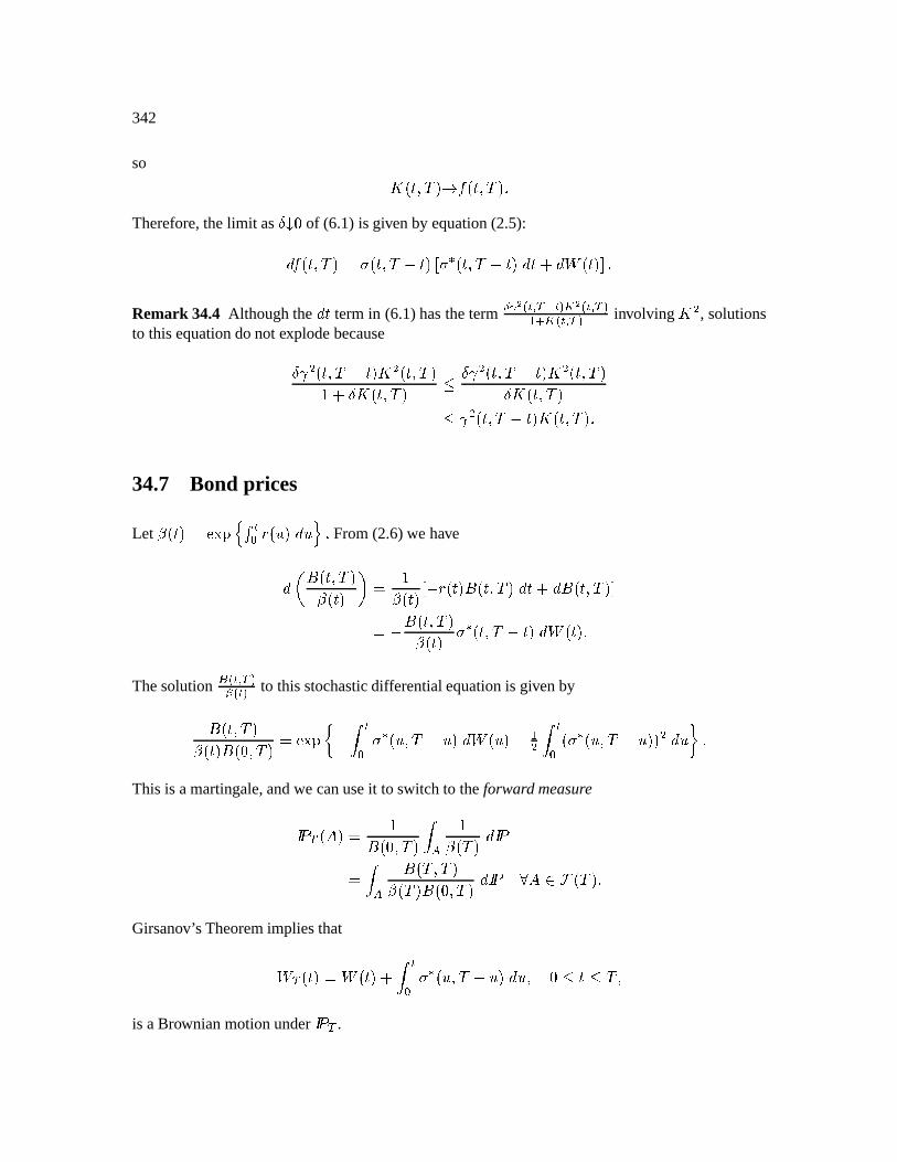
342
so _#öüøhô¶ýaç ¸ öüø/ô ýTherefore,thelimit as Ì × ÷ of (6.1) is givenby equation(2.5): ¸ öüø/ô ý=$ïöüø/ô|EüAý R $ ù öüøhôËE üAý ü#L 8( öüAýAú8Remark 34.4 Althoughthe ü termin (6.1)hastheterm ÒDèGé VU@ U êf é VU@ ` f U@ involving _ H , solutionsto thisequationdonot explodebecauseÌG6 H öüø/ôKEüAýa_ H öüø/ô¶ý L|ÌÓ_#öüø/ô¶ý Ì:6 H öüø/ô|E:üEýa_ H öüø/ô ýÌ_#öüø/ô¶ý|6 H öüø/ô|E üAýa_#öüø/ô¶ý34.7 Bond prices
Let öüEý sugv w Ð U ö@Zý Z y From(2.6)we have
<3 û öüø/ô ý öüAýë5 öüAý R ENöüAýhû öüø/ô¶ý üL û©öüøhô¶ý8úFE û©öüøhô¶ý öüAý $ ù öüøhô|E:üAý ( öüAýThesolution
U@ VU to thisstochasticdifferentialequationis givenbyû öüø/ô¶ý öüAýhû ö!÷øhô¶ý sugv n E U $ ù ö@ZøhôËEZý ( öDZý1E H U ö@$ ù ö@ZøhôËEZý/ý H Z p This is amartingale,andwe canuseit to switchto theforward measureþ ÿ ö ý û ö!÷èø/ô¶ý öô¶ý. þ ÿ û öô¶ø/ô ý öô¶ý/û©ö!÷ø/ô ý þ ÿ õ<¥öô ýGirsanov’sTheoremimpliesthat
( öüAýX ( öüEý#L U $ ù ö@Zøhô|E9Zý Zø ÷)ü#ô øis aBrownianmotionunder
þ ÿ.
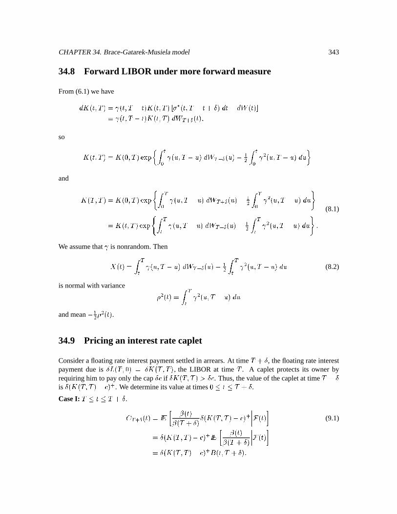
CHAPTER34. Brace-Gatarek-Musielamodel 343
34.8 Forward LIBOR under more forward measure
From(6.1)we have _#öüø/ô¶ý176ïöüøhôrE üAýa_#öüø/ô¶ý R $ ù öüøhô|E:üLKÌý üL ( öüEý8ú76ïöüøhôrE üAýa_#öüø/ô¶ý 8( `Ò öüAýøso _#öüø/ô¶ý1=_#ö!÷øhô¶ý suCv n U 6ïö@Zñø/ôrE9Z¼ý 8( `Ò öDZý1E H U 6 H ö@Zñø/ôErZý Z pand _ öô¶ø/ô ý#=_#ö!÷øhô¶ý suCvmº 6ïö@Zñø/ôrE9Z¼ý 8( `Ò öDZý1E H 6 H ö@Zñø/ô|ErZ¼ý Z1» (8.1)=_#öüøhô¶ý suCvmº U 6ïö@Zñø/ôErZý ( `Ò ö@ZýE H U 6 H ö@ZøhôËE9Z¼ý Z2»<We assumethat 6 is nonrandom.ThenöüAý U 6ïö@ZøhôrErZ¼ý 8( `Ò ö@Z¼ýE H U 6 H ö@Zñø/ô|E9Zý Z (8.2)
is normalwith variance H öüEý U 6 H ö@Zñø/ô|E9Zý ZandmeanE H H öüEý .34.9 Pricing an interestrate caplet
Considera floatingrateinterestpaymentsettledin arrears.At time ôrLKÌ , thefloatingrateinterestpaymentdue is Ìζöô ø÷NýæÌÓ_#öô ø/ô¶ýgø the LIBOR at time ô . A capletprotectsits owner byrequiringhim to payonly thecap ÌÄ if Ì_ öô¶ø/ô ýXk7ÌÄ . Thus,thevalueof thecapletat time ôrLOÌis Ìö@_#öô¶øhô¶ýE9Äý ` . We determineits valueat times ÷)ü#ôLOÌ .CaseI: ô=#üôrLOÌ .ì `Ò öüEý þ \ ] öüAý öôrL|Ìý Ìö@_#öô¶øhô¶ýErÄý ` ¼¼¼¼ £öüEý b (9.1)=Ìö@_#öô¶øhô¶ýErÄý ` þ \ ] öüAý öô9LOÌý ¼¼¼¼ £öüEý b=Ìö@_#öô¶øhô¶ýErÄýa`4û öüø/ôL|Ì,ý
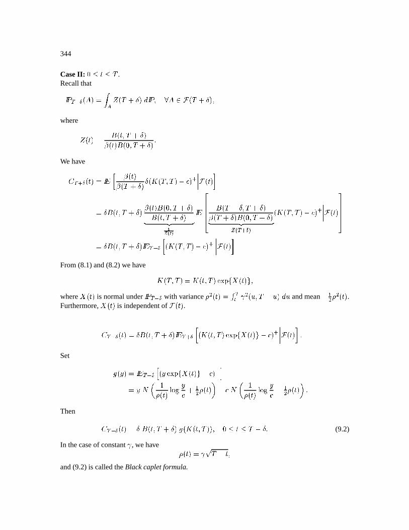
344
CaseII: ÷)#ü!#ô .Recallthatþ ÿ# `Ò ö ý )í öôLOÌý þ ÿ ø õ£öôrL|Ìýøwhere í öüAý û©öüøhôrLOÌý öüEý/û ö÷ø/ô9LOÌý We haveì `Ò öüEý þ \ ] öüAý öôrL|Ìý Ìö@_#öô ø/ô¶ýEÄýa`N¼¼¼¼ ¥öüAý b=Ìû öüø/ôrLKÌý öüAýhû ö!÷øhô9L|Ì,ýû öüø/ôrL|ÌýÀ Á Ãîïið·ñóò þ \ ßôôôôà û©öôrLKÌ&øhôÔLKÌý öôrLOÌý/û©ö!÷øhôõLOÌýÀ Á Ãö `Ò ö_#öô ø/ô¶ýE9Äý ` ¼¼¼¼ £öüAý â·÷÷÷÷ã=Ìû öüø/ôrLKÌý þ \ `Ò ] ö@_#öô¶øhô¶ý#E9Äý ` ¼¼¼¼ £öüAý bFrom(8.1)and(8.2)wehave _#öô¶øhô¶ý#=_#öüø/ô¶ý sugv *GöüAýø-øwhereöüEý is normalunder
þ ÿ# `Ò with variance H öüEýX Ð U 6 H öDZø/ô|EZý Z andmean E H H öüAý .Furthermore,öüAý is independentof öüAý .ì `Ò öüAý%Ì,û©öüøhôrLOÌý þ \N `Ò ] öª_#öüø/ô¶ý sugv *GöüEý-NE9Äý ` ¼¼¼¼ £öüAý b Set >ö@ùzý2 þ \N `Ò M ö@ù suCv *GöüAý-NE9Äý ` P%ùá 3 öüEý#Vi~ ù Ä L H öüAý 5 E9Ä! 3 öüAý1Vi~ ù Ä E H öüEý 5 Then ì `Ò öüAý%Ìeû öüø/ôrLKÌ,ý>ö@_#öüø/ô¶ý/ýgø ÷)#ü!#ôOErÌ: (9.2)
In thecaseof constant6 , wehave öüEý76 ôKE:üøand(9.2)is calledtheBlack capletformula.
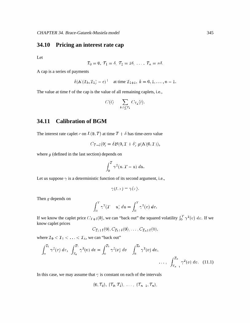
CHAPTER34. Brace-Gatarek-Musielamodel 345
34.10 Pricing an interestrate cap
Let ô l÷ø4ô =Ì&ø ô H =IÌ&øN:G¼øôúá=ûÌ:A capis a seriesof paymentsÌö@_#öô ø/ô ý1ErÄýa` at time ô ` ø l÷ø øG:øû<E Thevalueat time ü of thecapis thevalueof all remainingcaplets,i.e.,ì öüAý ¤ü UDý þ
ì þ öüAý34.11 Calibration of BGM
Theinterestratecaplet Ä on ζö!÷øhô¶ý at time ôrLOÌ hastime-zerovalueì `Ò ö÷Ný2%Ì,û©ö!÷øhôrL|Ìý>ñö@_#ö!÷èø/ô¶ý/ýgøwhere> (definedin thelastsection)dependson 6 H öDZø/ô|E9Z¼ý ZLet ussuppose6 is adeterministicfunctionof its secondargument,i.e.,6 öüøÅý76ïö@ÅýThen > dependson 6 H öô|EZý Z4 6 H ö@Ézý É'If we know thecapletprice
ì `Ò ö!÷Ný , we can“back out” thesquaredvolatility Ð 6 H ö@Ézý É . If weknow capletprices
ì :ÿ `Ò ö!÷Nýø ì î `Ò ö!÷Nýø:G:ø ì `Ò ö!÷Nýøwhereô o ô o :G o ôú , wecan“back out” :ÿ 6 H ö@Éý ɼø î:ÿ 6 H ö@Ézý Éz î 6 H ö@Ézý É.E :ÿ 6 H ö@Ézý Éø GG¼ø î 6 H ö@Ézý É; (11.1)
In thiscase,we mayassumethat 6 is constantoneachof theintervalsö!÷ø/ô ýgøÈöô ø/ô ýgøNG:ø¶öôú øhôúyýgø
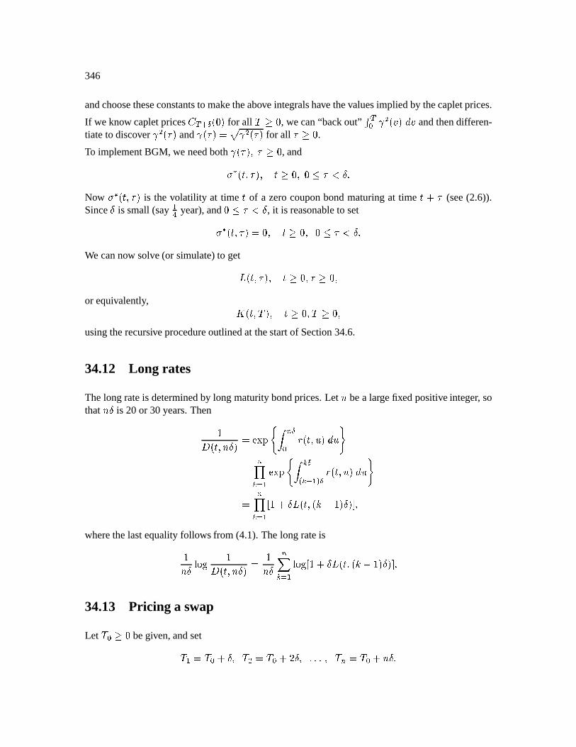
346
andchoosetheseconstantsto maketheabove integralshave thevaluesimpliedby thecapletprices.
If weknow capletprices
ì `Ò ö÷Ný for all ô=/÷ , wecan“backout” Ð 6 H ö@Ézý É andthendifferen-tiateto discover 6 H öDÅý and 6ïö@Åý1 6 H ö@Åý for all Å/÷ .To implementBGM, we needboth 6 öDÅýø2Å/s÷ , and$ ù öüøÅýgø ü!/÷øï÷)KÅ o Ì:Now $ ù öüøÅý is the volatility at time ü of a zerocouponbondmaturingat time ü L%Å (see(2.6)).SinceÌ is small(say Í year),and ÷OÅ o Ì , it is reasonableto set$ ù öüøÅý1l÷ø ü/÷èø:÷)OÅ o Ì:We cannow solve(or simulate)to getÎ öüøÅýø ü!/÷øÅ</÷øor equivalently, _ öüø/ô ýø ü/s÷ø/ô7/÷øusingtherecursiveprocedureoutlinedat thestartof Section34.6.
34.12 Long rates
Thelongrateis determinedby long maturitybondprices.Let û bea largefixedpositiveinteger, sothat ûÌ is 20or 30years.Then Ç öüøûÌý sugv¿º ú Ò öüøZý Z1» ú sugvzº Ò Ò öüøZ¼ý Z2» ú R L|Ìζöüø,ö@¿E ýÌ,ýAúøwherethelastequalityfollowsfrom (4.1).ThelongrateisûÌ Vi~ Ç öüøûÌý ûÌ ú¤ Vi~R LOÌÎ öüøö@zE ýaÌý8úQ34.13 Pricing a swap
Let ô /s÷ begiven,andsetô [ô L|̤ø:ô H Gô LOIi̤ø|G:ø:ôú)Gô L|ûÌ:
CHAPTER34. Brace-Gatarek-Musielamodel 347
Theswapis theseriesof paymentsÌ|öDζöô ø÷ý#ErÄý at time ô ` øáÒ÷ø ø:Gøû4E For ÷)#üô , thevalueof theswapisú ¤ þ \^] öüEý öô ` ý Ìö@ζöô ø÷Ný1E9Äý ¼¼¼¼ ¥öüAýDbmNow LOÌζöô ø÷Ný2 û öô ø/ô ` ý øso ζöô ø÷Ný2 Ì ] û öô ø/ô ` ý E bmWe compute þ \ ] öüAý öô ` ý Ì|öDζöô ø÷ý2EÄý ¼¼¼¼ £öüEý b þ \ ] öüEý öô ` ý 3 û©öô ø/ô ` ý E E9ÌÄ 5 ¼¼¼¼ öüAý b þ \ ßôôôôà öüEý öô ý/û©öô øhô ` ý þ \ ] öô ý öô ` ý ¼¼¼¼ £öô ý bÀ Á à þ Óþ î ¼¼¼¼ ¥öüAý â·÷÷÷÷ã EGö LOÌÄý/û©öüøhô ` ý
þ \ ] öüEý öô ` ý ¼¼¼¼ öüAý b Eö L|ÌÄý/û©öüøhô ` ýÒû öüø/ô ýEGö LOÌÄý/û©öüøhô ` ýThevalueof theswapat time ü isú ¤ þ \ ] öüAý öô ` ý Ìö@ζöô ø÷Ný#EÄý¼¼¼¼ £öüEý b ú ¤ R û öüø/ô ý2EGö LOÌÄý/û©öüøhô ` ýAúlû©öüøhô ýEö L|ÌÄý/û öüø/ô ý#L#û öüø/ô ýE ö L|ÌÄý/û©öüøhô H ý#L7:GLsû öüø/ôú ýEö L|ÌÄý/û öüø/ôúýlû©öüøhô ýE9ÌÄû©öüøhô ýE9ÌÄû öüø/ô H ýE|G:E9ÌÓÄû©öüøhô ú ýE:û öüø/ô ú ýThe forwardswaprate :ÿ öüAý at time ü for maturity ô is the valueof Ä which makesthe time-üvalueof theswapequalto zero:
:ÿ öüAý û©öüøhô ýE:û öüø/ôúýÌ R û öüø/ô ý#L7G:øL#û©öüøhô ú ý8ú In contrastto thecapformula,which dependson thetermstructuremodelandrequiresestimationof 6 , theswapformulais generic.

348
Chapter 35
Notesand References
35.1 Probability theory and martingales.
Probabilitytheoryis usuallylearnedin two stages.In thefirst stage,onelearnsthata discreteran-domvariablehasaprobabilitymassfunctionandacontinuousrandomvariablehasadensity. Thesecanbeusedtocomputeexpectationsandvariances,andevenconditionalexpectations.Furthermore,onelearnshow transformationsof continuousrandomvariablescausechangesin their densities.Awell-writtenbookwhichcontainsall thesethingsis DeGroot(1986).
The secondstageof probability theory is measuretheoretic. In this stageone views a randomvariableasa functionfrom a samplespace to thesetof realnumbers
þ . Certainsubsetsof are
calledevents, andthecollectionof all eventsformsa $ -algebra . Eachset
in hasaprobabilityþ ÿ ö ý . This point of view handlesbothdiscreteandcontinuousrandomvariableswithin thesameunifying framework. A conditionalexpectationis itself a randomvariable,measurablewith respectto theconditioning$ -algebra.Thispointof view is indispensiblefor treatingtherathercomplicatedconditionalexpectationswhicharisein martingaletheory. A well-writtenbookonmeasure-theoreticprobabilityis Billingsley (1986).A succinctbookonmeasure-theoreticprobabilityandmartingalesin discretetime is Williams (1991).A moredetailedbookis Chung(1968).
The measure-theoreticview of probability theorywasbegun by Kolmogorov (1933). The termmartingalewasapparentlyfirst usedby Ville (1939),althoughtheconceptdatesbackto 1934workof Levy. Thefirst completeaccountof martingaletheoryis Doob(1953).
35.2 Binomial assetpricing model.
Thebinomialassetpricing modelwasdevelopedby Cox,Ross& Rubinstein(1979). Accountsofthis modelcanbefoundin severalplaces,includingCox & Rubinstein(1985),Dothan(1990)andRitchken(1987). Many modelsarefirst developedandunderstoodin continuoustime, and thenbinomialversionsaredevelopedfor purposesof implementation.
349
350
35.3 Brownian motion.
In 1828RobertBrown observed irregularmovementof pollensuspendedin water. This motion isnow known to becausedby thebuffetingof thepollenby watermolecules,asexplainedby Einstein(1905). Bachelier(1900)usedBrownian motion (not geometricBrownianmotion)asa modelofstockprices,even thoughBrownian motion cantakenegative values.Levy (1939,1948)discov-eredmany of the nonintuitive propertiesof Brownian motion. The first mathematicallyrigorousconstructionof Brownianmotionwascarriedout by Wiener(1923,1924).
Brownianmotionandits propertiesarepresentedin anumeroustexts, includingBillingsley (1986).Thedevelopmentin thiscourseis asummaryof thatfoundin Karatzas& Shreve (1991).
35.4 Stochasticintegrals.
The integral with respectto Brownianmotion wasdevelopedby Ito (1944). It wasintroducedtofinanceby Merton(1969).A mathematicalconstructionof this integral,with a minimumof fuss,isgivenby Øksendal(1995).
Thequadraticvariationof martingaleswasintroducedby Fisk (1966)anddevelopedinto theformusedin thiscourseby Kunita& Watanabe(1967).
35.5 Stochasticcalculusand financial markets.
Stochasticcalculusbeginswith Ito (1944). Many financebooks,including(in orderof increasingmathematicaldifficulty) Hull (1993),Dothan(1990)andDuffie (1992), includesectionson Ito’sintegralandformula.Someotherbooksondynamicmodelsin financeareCox& Rubinstein(1985),Huang& Litzenberger (1988), Ingersoll (1987), and Jarrow (1988). An excellent referenceforpractitioners,now in preprintform, is Musiela& Rutkowski (1996). Somemathematicstexts onstochasticcalculusareØksendal(1995),Chung& Williams (1983),Protter(1990)andKaratzas&Shreve (1991).
Samuelson(1965,1973)presentsthe argumentthat geometricBrownian motion is a goodmodelfor stockprices.This is oftenconfusedwith theefficientmarkethypothesis, which assertsthatallinformationwhichcanbelearnedfromtechnicalanalysisof stockpricesis alreadyreflectedin thoseprices.Accordingto this hypothesis,paststockpricesmaybeusefulto estimatetheparametersofthedistributionof futurereturns,but they do not provide informationwhich permitsan investortooutperformthemarket.Themathematicalformulationof theefficientmarkethypothesisis thatthereis a probabilitymeasureunderwhich all discountedstockpricesaremartingales,a muchweakerconditionthanthe claim that stockpricesfollow a geometricBrownian motion. Someempiricalstudiessupportingthe efficient markethypothesisareKendall(1953),Osborne(1959),Sprenkle(1961), Boness(1964), Alexander(1961) and Fama(1965). The last of thesepapersdiscussesotherdistributionswhichfit stockpricesbetterthangeometricBrownianmotion.A criticismof theefficient markethypothesisis provided by LeRoy (1989). A provocative article on the sourceof
CHAPTER35. NotesandReferences 351
stockpricemovementsis Black(1986).
The first derivation of the Black-Scholesformula given in this course,usingonly Ito’s formula,is similar to that originally givenby Black & Scholes(1973). An importantcompanionpaperisMerton (1973),which makesgoodreadingeven today. (This andmany otherpapersby Mertonarecollectedin Merton (1990).) Even thoughgeometricBrownian motion is a lessthanperfectmodelfor stockprices,theBlack-Scholesoptionhedgingformulaseemsnot to bevery sensitivetodeficienciesin themodel.
35.6 Mark ov processes.
Markov processeswhich aresolutionsto stochasticdifferentialequationsarecalleddiffusionpro-cesses. A goodintroductionto this topic, including discussionsof the Kolmogorov forward andbackwardequations,is Chapter15 of Karlin & Taylor (1981). The otherbookscited previously,Øksendal(1995),Protter(1990),Chung& Williams (1983),andKaratzas& Shreve(1991),all treatthis subject.Kloeden& Platen(1992)is a thoroughstudyof the numericalsolutionof stochasticdifferentialequations.
Theconstantelasticityof variancemodelfor optionpricingappearsin Cox& Ross(1976).Anotheralternative modelfor the stockpriceunderlyingoptions,dueto Follmer & Schweizer(1993),hasthegeometricOrnstein-Uhlenbeckprocessasaspecialcase.
TheFeynman-KacTheorem,connectingstochasticdifferentialequationstopartialdifferentialequa-tions, is dueto Feyman(1948)andKac (1951). A numericaltreatmentof the partial differentialequationsarisingin financeis containedin Wilmott, DewynneandHowison(1993,1995)andalsoDuffie (1992).
35.7 Girsanov’stheorem,the martingale representationtheorem,andrisk-neutral measures.
Girsanov’sTheoremin thegeneralitystatedhereis dueto Girsanov (1960),althoughtheresultforconstant wasestablishedmuch earlierby Cameron& Martin (1944). The theoremrequiresatechnicalconditionto ensurethat
þ \ í öô¶ý , sothat þ ÿ is a probabilitymeasure;seeKaratzas&Shreve (1991),page198.
The form of the martingalerepresentationtheorempresentedhereis from Kunita & Watanabe(1967).It canalsobefoundin Karatzas& Shreve (1991),page182.
Theapplicationof theGirsanov Theoremandthemartingalerepresentationtheoremto risk-neutralpricing is dueto Harrison& Pliska(1981). This methodologyfreesthe Brownian-motiondrivenmodelfrom theassumptionof constantinterestrateandvolatility; theseparameterscanberandomthroughdependenceonthepathof theunderlyingasset,or eventhroughdependenceonthepathsofotherassets.Whenboththe interestrateandvolatility of anassetareallowedto bestochastic,theBrownian-motiondrivenmodelis mathematicallythemostgeneralpossiblefor assetpriceswithoutjumps.
352
When assetprocesseshave jumps, risk-freehedgingis generallynot possible. Someworks onhedgingand/oroptimizationin modelswhich allow for jumpsareAase(1993),Back(1991),Bates(1988,1992),Beinert& Trautman(1991),Elliott & Kopp(1990),Jarrow & Madan(1991b,c),Jones(1984),Madan& Seneta(1990),Madan& Milne (1991),Mercurio& Runggaldier(1993),Merton(1976),Naik & Lee(1990),Schweizer(1992a,b),Shirakawa(1990,1991)andXue(1992).
TheFundamentalTheoremof AssetPricing,asstatedhere,canbefoundin Harrison& Pliska(1981,1983). It is temptingto believe theconverseof Part I, i.e., thattheabsenceof arbitrageimpliestheexistenceof a risk-neutralmeasure.This is true in discrete-timemodels,but in continuous-timemodels,aslightly strongerconditionis neededto guaranteeexistenceof arisk-neutralmeasure.Forthe continuous-timecase,resultshave beenobtainedby many authors,including Stricker(1990),Delbaen(1992),Lakner(1993),Delbaen& Schachermayer(1994a,b),andFritelli & Lakner(1994,1995).
In additionto the fundamentalpapersof Harrison& Kreps(1979),andHarrison& Pliska(1981,1983),someotherworkson the relationshipbetweenmarketcompletenessanduniquenessof therisk-neutralmeasureareArtzner& Heath(1990),Delbaen(1992),Jacka(1992),Jarrow & Madan(1991a),Muller (1989)andTaqqu& Willinger (1987).
35.8 Exotic options.
Thereflectionprinciple,adjustedto accountfor drift, is takenfrom Karatzas& Shreve(1991),pages196–197.
Explicit formulasfor thepricesof barrieroptionshavebeenobtainedby Rubinstein& Reiner(1991)andKunitomo& Ikeda(1992). Lookbackoptionshave beenstudiedby Goldman,Sosin& Gatto(1979),Goldman,Sosin& Shepp(1979)andConze & Viswanathan(1991).
Becauseit is difficult to obtainexplicit formulasfor the pricesof Asian options,mostwork hasbeendevotedto approximations.We do not provide anexplicit pricing formulahere,althoughthepartialdifferentialequationgivenhereby theFeynman-KacTheoremcharacterizestheexactprice.Bouaziz,Bryis & Crouhy(1994)provide an approximatepricing formula, Rogers& Shi (1995)providea lowerbound,andGeman& Yor (1993)obtaintheLaplacetransformof theprice.
35.9 American options.
A generalarbitrage-basedtheoryfor thepricingof Americancontingentclaimsandoptionsbeginswith the articlesof Bensoussan(1984)andKaratzas(1988);seeMyneni (1992)for a survey andadditionalreferences.TheperpetualAmericanput problemwassolvedby McKean(1965).
Approximationand/ornumericalsolutionsfor the Americanoption problemhave beenproposedby several authors,including Black (1975),Brennan& Schwartz(1977)(seeJaillet et al. (1990)for atreatmentof theAmericanoptionoptimalstoppingproblemvia variationalinequalities,whichleadsto a justificationof theBrennan-Schwartzalgorithm),by Cox,Ross& Rubinstein(1979)(seeLamberton(1993)for theconvergenceof theassociatedbinomialand/orfinite differenceschemes)
CHAPTER35. NotesandReferences 353
andby Parkinson(1977),Johnson(1983),Geske& Johnson(1984),MacMillan (1986),Omberg(1987),Barone-Adesi& Whalley (1987),Barone-Adesi& Elliott (1991),Bunch& Johnson(1992),Broadie& Detemple(1994),andCarr& Faguet(1994).
35.10 Forward and futur escontracts.
The distinctionbetweenfuturescontractsanddaily resettledforward contractshasonly recentlybeenrecognized(seeMargrabe(1976),Black (1976))andeven morerecentlyunderstood.Cox,Ingersoll& Ross(1981)andJarrow & Oldfield(1981)provideadiscrete-timearbitrage-basedanal-ysisof therelationshipbetweenforwardsandfutures,whereasRichard& Sundaresan(1981)studytheseclaimsin acontinuous-time,equilibriumsetting.Ourpresentationof thismaterialis similar tothatof Duffie & Stanton(1992),which alsoconsidersoptionson futures,andto Chapte7 of Duffie(1992).For additionalreadingon forwardandfuturescontracts,onemayconsultDuffie (1989).
35.11 Term structur emodels.
TheHull & White(1990)modelis ageneralizationof theconstant-coefficentVasicek(1977)model.Implementationsof themodelappearin Hull & White(1994a,b).TheCox-Ingersoll-Rossmodelispresentedin (1985a,b).Thepresentationsof thesegivenmodelshereis takenfrom Rogers(1995).Othersurveysof termstructuremodelsareDuffie & Kan(1994)andVetzal(1994).A partial list ofothertermstructuremodelsis Black,Derman& Toy (1990),Brace& Musiela(1994a,b),Brennan& Schwartz(1979,1982)(but seeHogan(1993)for discussionof aproblemwith thismodel),Duffie& Kan(1993),Ho & Lee(1986),Jamshidian(1990),andLongstaff & Schwartz(1992a,b).
Thecontinuous-timeHeath-Jarrow-Mortonmodelappearsin Heath,Jarrow & Morton (1992),anda discrete-timeversionis providedby Heath,Jarrow & Morton (1990). Carverhill & Pang(1995)discussimplementation.The Brace-Gatarek-Musielavariationof the HJM model is takenfromBrace,et al. (1995). A summaryof this modelappearsasReed(1995). Relatedworks on termstructuremodelsandswapsareFlesaker& Hughston(1995)andJamshidian(1996).
35.12 Changeof numeraire.
Thismaterialin thiscourseis takenfrom Geman,El KarouiandRochet(1995).Similar ideaswereusedby by Jamshidian(1989).TheMertonoptionpricing formulaappearsin Merton(1973).
35.13 Foreignexchangemodels.
Foreignexchangeoptionswerepricedby Biger & Hull (1983)andGarman& Kohlhagen(1983).Thepricesfor differentialswapshave beenworkedout by Jamshidian(1993a,1993b)andBrace&Musiela(1994a).
354
35.14 REFERENCES
(1993)Aase,K. K., A jump/diffusionconsumption-basedcapitalassetpricingmodelandtheequitypremiumpuzzle,Math.Finance3(2), 65–84.
(1961)Alexander, S. S.,Pricemovementsin speculative markets:trendsor randomwalks, Indus-trial ManagementReview 2, 7–26.Reprintedin Cootner(1964),199–218.
(1990)Artzner, P. & Heath,D., Completenessandnon-uniquepricing, preprint,Schoolof Opera-tionsResearchandIndustrialEngineering,CornellUniversity.
(1900)Bachelier, L., Theoriede la speculation,Ann.Sci.EcoleNorm.Sup. 17, 21–86.Reprintedin Cootner(1964).
(1991)Back,K., Assetpricing for generalprocesses,J. Math.Econonics20, 371–395.
(1991)Barone-Adesi,G. & Elliott, R., Approximationsfor thevaluesof Americanoptions,Stoch.Anal.Appl. 9, 115–131.
(1987)Barone-Adesi,G. & Whalley, R., Efficient analyticapproximationof Americanoptionval-ues,J. Finance42, 301–320.
(1988)Bates,D. S., Pricingoptionsunderjump-diffusionprocesses,preprint,WhartonSchoolofBusiness,Universityof Pennsylvania.
(1992)Bates,D. S., Jumpsandstochasticvolatility: exchangerateprocessesimplicit in foreigncurrency options,preprint,WhartonSchoolof Business,Universityof Pennsylvania.
(1991)Beinert,M. & Trautmann,S.,Jump-diffusionmodelsof stockreturns:astatisticalinvestiga-tion, StatistischeHefte32, 269–280.
(1984)Bensoussan,A., On thetheoryof optionpricing,ActaAppl.Math. 2, 139–158.
(1983)Biger, H. & Hull, J., The valuationof currency options,Financial Management, Spring,24–28.
(1986)Billingsley, P., ProbabilityandMeasure, 2ndedition,Wiley, New York.
(1975)Black,F., Factandfantasyin theuseof options,FinancialAnalyst’sJ., 31, 36–41,61–72.
CHAPTER35. NotesandReferences 355
(1976)Black,F., Thepricingof commoditycontracts,J. FinancialEconomics3.
(1986)Black,F., Noise,J. Finance41, 529–543.
(1990)Black,F., Derman,E. & Toy, W., A one-factormodelof interestratesandits applicationtotreasurybondoptions,Fin. Anal.Journal, 33–39.
(1973)Black,F. & Scholes,M., Thepricingof optionsandcorporateliabilities,J. Political Economy81, 637–659.
(1964)Boness,Someevidenceof theprofitabilityof tradingputandcall options.In Cootner(1964),475–496.
(1994) Bouaziz,L., Bryis, E. & Crouhy, M., The pricing of forward-startingAsian options,J.BankingFinance.
(1994a)Brace,A. & Musiela,M., Swapderivativesin aGaussianHJM framework,preprint,Schoolof Mathematics,Universityof New SouthWales.
(1994b)Brace,A. & Musiela,M., A multi-factorGaussMarkov implementationof Heath,JarrowandMorton,Math. Finance4, 259–283.
(1995)Brace,A.. Gatarek,D. & Musiela,M., Themarketmodelof interestratedynamics,preprint,Schoolof Mathematics,Universityof New SouthWales.
(1977)Brennan,M. J.& Schwartz,E. S.,Thevaluationof theAmericanput option,J. Finance32,449–462.
(1979)Brennan,M. J. & Schwartz,E. S.,A continuous-timeapproachto thepricing of bonds,J.BankingFinance3, 133–155.
(1982)Brennan,M. J.& Schwartz,E.S.,An equilibriummodelof bondpricingandatestof marketefficiency, J. FinancialQuantitativeAnalysis17, 301–329.
(1994)Broadie,M. & Detemple,J., Americanoption values:new bounds,approximationsandacomparisonof existingmethods,preprint,GraduateSchoolof Business,ColumbiaUniversity.
(1992)Bunch,D. & Johnson,H., A simpleandnumericallyefficientvaluationmethodfor Americanputs,usinga modifiedGeske-Johnsonapproach,J. Finance47, 809–816.
(1944)Cameron,R. H. & Martin, W. T., Transformationof Wiener integralsundertranslations,
356
Ann.Math. 45, 386–396.
(1994)Carr, P. & Faguet,D., Fastaccuratevaluationof Americanoptions,preprint,JohnsonSchoolof Business,CornellUniversity.
(1995)Carverhill, A. & Pang,K., Efficientandflexible bondoptionvaluationin theHeath,Jarrow,andMorton framework, J. FixedIncome, September, 70–77.
(1968)Chung,K. L. A Coursein ProbabilityTheory, AcademicPress,Orlando,FL.
(1983)Chung,K. L. & Williams, R. J. (1983)Introductionto StochasticIntegration, Birkhauser,Boston.
(1991)Conze, A. & Viswanathan,R., Path dependentoptions: the caseof lookbackoptions,J.Finance46, 1893–1907.
(1964)Cootner, P. H. (editor),TheRandomCharacter of Stock Market Prices, MIT Press,Cam-bridge,MA.
(1981)Cox,J.C., Ingersoll,J.E.,& Ross,S,Therelationbetweenforwardpricesandfuturesprices,J. FinancialEconomics9, 321–346.
(1985a)Cox,J.C., Ingersoll,J.E. & Ross,S.,An intertemporalgeneralequilibriummodelof assetprices,Econometrica53, 363–384.
(1985b)Cox, J. C., Ingersoll, J. E. & Ross,S., A theoryof the term structureof interestrates,Econometrica53, 373–384.
(1976)Cox,J.C. & Ross,S.A., Thevaluationof optionsfor alternativestochasticprocesses,J. Fin.Economics3, 145–166.
(1979)Cox,J.C.,Ross,S.A. & Rubinstein,M., Optionpricing: asimplifiedapproach,J. FinancialEconomics7, 229–263.
(1985)Cox,J.C. & Rubinstein,M. OptionsMarkets, PrenticeHall, EnglewoodClif fs, NJ.
(1986)DeGroot,M., ProbabilityandStatistics, 2ndedition,AddisonWesley, Reading,MA.
(1992)Delbaen,F., Representingmartingalemeasureswhenassetpricesarecontinuousandbounded,Math.Finance2(2), 107–130.
CHAPTER35. NotesandReferences 357
(1994a)Delbaen,F. & Schachermayer, W., A generalversionof thefundamentaltheoremof assetpricing,MathematischeAnnalen300, 463–520.
(1994b)Delbaen,F. & Schachermayer, W., Arbitrageand free-lunchwith boundedrisk, for un-boundedcontinuousprocesses,Math.Finance4(4), 343–348.
(1953)Doob,J.,StochasticProcesses, Wiley, New York.
(1990)Dothan,M. U., Pricesin FinancialMarkets, OxfordUniversityPress,New York.
(1989)Duffie,D., FuturesMarkets, Prentice-Hall,EnglewoodClif fs, NJ.
(1992)Duffie,D., DynamicAssetPricing Theory, PrincetonUniversityPress,Princeton.
(1993)Duffie,D. & Kan,R.,A yield-factormodelof interestrates,preprint.
(1994)Duffie, D. & Kan,R., Multi-factor termstructuremodels,Phil. TransactionsRoyalSocietyLondonA 347, 577–586.
(1992) Duffie, D. & Stanton,R., Pricing continuouslyresettledcontingentclaims, J. EconomicDynamicsandControl, 16, 561–573.
(1905)Einstein,A. On themovementof smallparticlessuspendedin a stationaryliquid demandedby themolecular-kinetic theoryof heat,Ann.Physik17.
(1990)Elliott, R.J.& Kopp,P. E.,Optionpricingandhedgeportfoliosfor Poissonprocesses,Stoch.Anal. Appl. 9, 429–444.
(1965)Fama,E. Thebehavior of stock-marketprices,J. Business38, 34–104.
(1948)Feynman,R., Space-timeapproachto nonrelativistic quantummechanics,Rev. Mod. Phys.20, 367–387.
(1966)Fisk,D. L., Samplequadraticvariationof continuous,second-ordermartingales,Z.Wahrschein-lichkeitstheorieverw. Gebiete6, 273–278.
(1995)Flesaker, B. & Hughston,L., Positiveinterest,preprint.
(1993)Follmer, H. & Schweizer, M., A microeconomicapproachto diffusion modelsfor stockprices,Math. Finance3, 1–23.
358
(1994)Fritelli, M. & Lakner, P., Almost surecharacterizationof martingales,Stochastics49, 181–190.
(1995)Fritelli, M. & Lakner, P., Arbitrageandfree-lunchin a generalfinancemarketmodel: thefundamentaltheoremof assetpricing, IMA Vol 65: MathematicalFinance, 89–92,(M. Davis, D.Duffie, W. Fleming& S.Shreve,eds.),Springer-Verlag,New York.
(1983)Garman,M. & Kohlhagen,S., Foreigncurrency option values,J. InternationalMoney Fi-nance2, 231–237.
(1995)Geman,H., El Karoui, N. & Rochet,J.-C.,Changesof numeraire,changesof probabilitymeasure,andoptionpricing,J. AppliedProbability32, 443–458.
(1993) Geman,H. & Yor, M., Besselprocesses,Asian options,and perpetuities,MathematicalFinance3, 349–375.
(1984)Geske,R.& Johnson,H., TheAmericanput-optionvaluedanalytically, J. Finance39, 1511–1524.
(1960)Girsanov, I. V., Ontransformingacertainclassof stochasticprocessesby absolutelycontin-uoussubstitutionof measures,TheoryProbabilityApplications5, 285–301.
(1979)Goldman,B., Sosin,H. & Gatto,M., Path dependentoptions: “Buy at the low, sell at thehigh,” J. Finance34, 69–84.
(1979)Goldman,B., Sosin,H. & Shepp,L. A., On contingentclaimsthat insureex-postoptimalstockmarkettiming, J. Finance34, 401–414.
(1979)Harrison,J.M. & Kreps,D. M., Martingalesandarbitragein multiperiodsecuritiesmarkets,J. EconomicTheory20, 381–408.
(1981)Harrison,J.M. & Pliska,S.R.,Martingalesandstochasticintegralsin thetheoryof contin-uoustrading,StochasticProcessesApplications11, 215–260.
(1983)Harrison,J.M. & Pliska,S.R.,A stochasticcalculusmodelof continuoustrading:completemarkets,StochasticProcessesApplications15, 313–316.
(1990)Heath,D., Jarrow, R. & Morton,A., Bondpricing andthetermstructureof interestrates:adiscretetimeapproximation,J. FinancialQuantitativeAnalysis25, 419–440.
(1992)Heath,D., Jarrow, R. & Morton,A., Bondpricing andthetermstructureof interestrates:a
CHAPTER35. NotesandReferences 359
new methodology, Econometrica60, 77–105.
(1993)Hogan,M., Problemsin certaintwo-factortermstructuremodels,AnnalsAppliedProbability3, 576–581.
(1986)Ho, T. S. Y. & Lee, S.-B., Term structuremovementsandpricing interestratecontingentclaims,J. Finance41, 1011–1029.
(1988)Huang,C.-f. & Litzenberger, R., Foundationsfor Financial Economics, North Holland,Amsterdam.
(1993)Hull, J.,Options,Futures,andotherDerivativeSecurities, PrenticeHall, EnglewoodClif fs,NJ.
(1990)Hull, J. & White, A., Pricing interestratederivative securities,Rev. Financial Studies3,573–592.
(1994a)Hull, J. & White, A., Numericalproceduresfor implementingterm structuremodelsI:single-factormodels,J. Derivatives, Fall, 7–16.
(1994b)Hull, J.& White,A., Numericalproceduresfor implementingtermstructuremodelsII: twofactormodels,J. Derviatives, Winter.
(1987)Ingersoll,J.E.,Theoryof FinancialDecisionMaking, Rowman& Littlefield.
(1944)Ito, K., Stochasticintegral,Proc.ImperialAcad.Tokyo20, 519–524.
(1992)Jacka,S.,A martingalerepresentationresultandanapplicationto incompletefinancialmar-kets,Math.Finance2, 239–250.
(1990)Jaillet,P., Lamberton,D. & Lapeyre,B., Variationalinequaltiiesandthepricingof Americanoptions,ActaAppl.Math. 21, 263–289.
(1989)Jamshidian,F., An exactbondoptionpricing formula,J. Finance44, 205–209.
(1990)Jamshidian,F., Thepreference-freedeterminationof bondandoptionpricesfrom thespotinterestrate,AdvancesFutures& OptionsResearch 4, 51–67.
(1993a)Jamshidian,F., Pricedifferentials,RiskMagazine6/7.
360
(1993b)Jamshidian,F., Corrallingquantos,RiskMagazine7/3.
(1996)Jamshidian,F., Sortingoutswaptions,RiskMagazine9/3, 59–60.
(1988)Jarrow, R.,FinanceTheory, PrenticeHall, EnglewoodClif fs, NJ.
(1991a)Jarrow, R. & Madan,D., A characterizationof completesecuritymarketson a Brownianfiltration, Math.Finance1(3), 31–43.
(1991b)Jarrow, R. & Madan,D., Valuing and hedgingcontingentclaims on semimartingales,preprint,JohnsonSchoolof Business,CornellUniversity.
(1991c)Jarrow, R. & Madan,D., Optionpricing usingthetermstructureof interestratesto hedgesystematicdiscontinuitiesin assetreturns,preprint,JohnsonSchoolof Business,CornellUniversity.
(1981)Jarrow, R. & Oldfield, G., Forwardcontractsandfuturescontracts,J. Financial Economics9, 373–382.
(1983)Johnson,H., An analyticapproximationfor the Americanput price, J. Financial Quant.Analysis18, 141–148.
(1984)Jones,E. P., Optionarbitrageandstrategy with largepricechanges,J. FinancialEconomics13, 91–113.
(1951)Kac,M., Onsomeconnectionsbetweenprobabilitytheoryanddifferentialandintegralequa-tions,Proc.2ndBerkeley SymposiumonMath.Stat.& Probability, 189–215.
(1988)Karatzas,I., On thepricingof Americanoptions,App.Math. Optimization17, 37–60.
(1991)Karatzas,I. & Shreve, S. E., BrownianMotion and StochasticCalculus, Springer-Verlag,New York.
(1981) Karlin, S. & Taylor, H. M., A SecondCoursein Stochastic Processes, AcademicPress,Orlando,FL.
(1953)Kendall,M. G.,Analysisof economictime-series– Part I: prices,J. RoyalStatisticalSociety96,Part I , 11–25.Reprintedin Cootner(1964),85–99.
(1992)Kloeden,P. E.& Platen,E.,NumericalSolutionofStochasticDifferentialEquations,Springer-Verlag,New York.
CHAPTER35. NotesandReferences 361
(1933) Kolmogorov, A. N., Grundbegriffe der Wahrscheinlichkeitsrechnung, ErgebnisseMathe-matik2. Englishtranslation:Foundationsof ProbabilityTheory, Chelsea,New York, 1950.
(1967)Kunita, H. & Watanabe,S., On square-integrablemartingales,NagoyaMath. Journal 30,209–245.
(1992)Kunitomo,N. & Ikeda,M., Pricingoptionswith curvedboundaries,MathematicalFinance2, 275–298.
(1993)Lakner, P., Martingalemeasuresfor a classof right-continuousprocesses,Math.Finance3,43–53.
(1993)Lamberton,D., Convergenceof thecritical pricein theapproximationof Americanoptions,Math.Finance3, 179–190.
(1989)LeRoy, S. F., Efficient capitalmarketsandmartingales,J. EconomicLiterature 27, 1583–1621.
(1939)Levy, P., Surcertainsprocessusstochastiqueshomogenes,CompositioMath. 7, 283–339.
(1948)Levy, P., ProcessusStochastiqueset MouvementBrownian, Gauthier-Villars, Paris.
(1992a)Longstaff, F. A. & Schwartz,E. S., Interestratevolatility andthe term structure:a two-factorgeneralequilibriummodel,J. Finance47, 1259–1282.
(1992b)Longstaff, F. A. & Schwartz,E. S.,A two-factorinterestratemodelandcontingentclaimvaluation,J. FixedIncome3, 16–23.
(1986)MacMillan, L., Analytic approximationfor theAmericanput option,Adv. FuturesOptionsResearch 1, 119–139.
(1990)Madan,D. & Seneta,E.,TheV. G. modelfor sharereturns,J. Business63, 511–524.
(1991)Madan,D. & Milne, F., Optionpricing with V. G. martingalecomponents,Math. Finance1(4), 39–56.
(1976)Margrabe,W., A theoryof forwardandfuturesprices,preprint,WhartonSchoolof Business,Universityof Pennsylvania.
(1965)McKean,H. P., Jr., Appendixto P. A. Samuelson(1965): A freeboundaryproblemfor theheatequationarisingfrom a problemin mathematicaleconomics,Industrial ManagementReview
362
6, 32–39.
(1993)Mercurio, F. & Runggaldier, W., Option pricing for jump diffusions: approximationsandtheir interpretation,Math. Finance3, 191–200.
(1969)Merton, R. C., Lifetime portfolio selectionunderuncertainty: the continuous-timecase,Review EconomicsStatistics51, 247–257.
(1973)Merton,R. C.,Theoryof rationaloptionpricing,Bell J. Econ.ManagementScience4, 141–183.
(1976)Merton,R. C.,Optionpricingwhenunderlyingstockreturnsarediscontinuous,J. Fin. Eco-nomics3, 125–144.
(1990)Merton,R. C., Continuous-TimeFinance, BasilBlackwell,Cambridge,1990.
(1989)Muller, S.On completesecuritiesmarketsandthemartingalepropertyon securitiesprices,EconomicLetters3137–41.
(1996) Musiela, M. & Rutkowski, M., ArbitragePricing of Derivative Securities. TheoryandApplications, Springer-Verlag,New York, to appear.
(1992)Myneni,R.,Thepricingof theAmericanoption,Ann.AppliedProbability2, 1–23.
(1990)Naik, V. & Lee, M., Generalequilibrium pricing of optionson the marketportfolio withdiscontinuousreturns,Rev. FinancialStudies3, 493–521.
(1995)Øksendal,B., StochasticDifferentialEquations, 4thEdition,Springer-Verlag,New York.
(1987)Omberg, E.,Thevaluationof Americanputswith exponentialexercisepolicies,Adv. FuturesOptionResearch 2, 117–142.
(1959)Osborne,M. F. M., Brownianmotionin thestockmarket,OperationsResearch 7, 145–173.Reprintedin Cootner(1964),100–128.
(1977)Parkinson,M., Optionpricing: theAmericanput,J. Business50, 21–36.
(1990)Protter, P., StochasticIntegrationandDifferentialEquations, Springer-Verlag,New York.
(1995)Reed,N., If thecapfits :G , Risk8(8), 34–35.
CHAPTER35. NotesandReferences 363
(1981) Richard,S. F. & Sundaresan,M., A continuous-timeequilibrium model of forward andfuturespricesin a multigoodeconomy, J. FinancialEconomics, 9, 347–371.
(1987)Ritchken,P. Options:Theory, StrategyandApplications, HarperCollins.
(1995)Rogers,L. C. G., Which modelof term-structureof interestratesshouldoneuse?,IMAVol. 65: MathematicalFinance, 93–116,(M. Davis, D. Duffie, W. Fleming& S. Shreve, editors),Springer-Verlag,New York.
(1995)Rogers,L. C. G. & Shi,Z., Thevalueof anAsianoption,J. AppliedProbability, to appear.
(1991)Rubinstein,M. & Reiner, E.,Breakingdown thebarriers,RiskMagazine4/8, 28–35.
(1965)Samuelson,P. A., Proofthatproperlyanticipatedpricesfluctuaterandomly, IndustrialMan-agementReview 4, 41–50.
(1973)Samuelson,P. A., Mathematicsof speculativeprices,SIAMReview 15, 1–42.
(1992a)Schweizer, M., Martingaledensitiesfor generalassetprices,J. Math.Economics21, 123–131.
(1992b)Schweizer, M., Mean-variancehedgingfor generalclaims,AnnalsAppl. Probab. 2, 171–179.
(1990)Shirakawa, H., Optimal dividendandportfolio decisionswith Poissonanddiffusion-typereturnprocesses,preprintIHSS90-20,Tokyo Instituteof Technology.
(1991)Shirakawa, H., Interestrateoption pricing with Poisson-Gaussianforward ratecurve pro-cesses,Math.Finance1(4), 77–94.
(1961)Sprenkle,C.M., Warrantpricesasindicatorsof expectationsandpreferences,YaleEconomicEssays1, 178–231.Reprintedin Cootner(1964),412–474.
(1990)Stricker, C.,Arbitrageet lois demartingales,Ann. Inst. henri Poincare26, 451–460.
(1987)Taqqu,M. & Willinger, W., Theanalysisof finite securitymarketsusingmartingales,Adv.Appl.Probab. 19, 1–25.
(1977)Vasicek,O., An equilibriumcharacterizationof the termstructure,J. Financial Economics5, 177–188.
364
(1994)Vetzal,K. R.,A survey of stochasticcontinuoustimemodelsof thetermstructureof interestrates,Insurance:MathematicsandEconomics14, 139–161.
(1939)Ville, J.,EtudeCritiquedela NotionduCollectif, Gauthier-Villars, Paris.
(1923)Wiener, N., Dif ferentialspaces,J. Math.Physics2, 131–174.
(1924)Wiener, N., Un problemedeprobabilitesdenombrables,Bull. Soc.Math. France52, 569–578.
(1991)Williams, D., Probabilitywith Martingales, CambridgeUniversityPress,Cambridge.
(1993)Wilmott, P., Dewynne,J. & Howison,S.,OptionPricing, Oxford FinancialPress,POBox348,Oxford,OX4 1DR,UK.
(1995)Wilmott, P., Dewynne,J. & Howison,S.,TheMathematicsof Financial Derivatives, Cam-bridgeUniversityPress,Cambridge.
(1992)Xue,X. X., Martingalerepresentationfor a classof processeswith independentincrements,andits applications,in Lecture Notesin Control andInformationSciences177, 279–311,Springer-Verlag,Berlin.