Embed Size (px)
Citation preview

NBER WORKING PAPER SERIES
TEST SCORES AND SELF—SELECTION OF HIGHEREDUCATION: COLLEGE ATTENDANCE VERSUS
COLLEGE COMPLETION
Steven Venti
David A. Wise
Working Paper No. 109
NATIONAL BUREAU OF ECONOMIC RESEARCH1050 Massachusetts Avenue
Cambridge MA 02138
July 1981
We are indebted to David Eliwood, Win Fuller, Jerry Hausman,Charles Manski, and Michael Stoto for their comments. This workwas supported by the Exxon Educational Foundation, contract number300—18—051-t5 from the Office of Education; Department of Health,Education, and Welfare; and the National Science Foundation. Theresearch reported here is part of the NBER's research program inLabor Studies. Any opinions expressed are those of the authors andnot those of the National Bureau of Economic Research.
NBER Working Paper #709July 1981
Test Scores and Self-Selection of Higher Education:
College Attendance Versus College Completion
ABSTRACT
As a companion paper to our work on students' application and colleges'
admission decisions, we have estimated a joint discrete-continuous utility
maximization model of college attendance and college completion. The paper
is motivated by the possibility that test scores are poor predictors of who
will succeed in college and thus may not promote optimal investment decisions
and may indeed unjustly limit the educational opportunities of some youth.
We find that: (1) College attendance decisions are strongly commensurate with
college completion. Persons who are unlikely to attend college would be very
likely to drop out of even their "first-choice" colleges, were they to attend.
College human capital investment decisions are strongly mirrored by the likeli-
hood that they will pay off. (2) Contrary to much of the recent criticism of
the predictive validity of test scores, we find that their informational
content is substantial. After controlling for high school class rank, for
example, the probability of dropping out of the first-choice college varies
greatly with SAT scores. (3) Individual self-selection, related to both
measured and unmeasured atrributes, is the dominant determinant of college
attendance.
Steven VentiJ.F.K. School of GovernmentHarvard UniversityCambridge, Massachusetts 02138
(617) 495-1456
Professor David A. WiseJ.F.K. School of GovernmentHarvard UniversityCambridge, Massachusetts 02138
(617) 495-1178

TEST SCORES AND SELF-SELECTION OF HIGHER EDUCATION:
COLLEGE ATTENDANCE VERSUS COLLEGE COMPLETION
by
Steven Venti and David A. Wise*
Most economic studies of college attendance emphasize the returns to
higher education as the motivation for an individual's choice to go to
college, but ignore institutional constraints on possible choices. Critics
of the use of test scores in the determination of college attendance on the
other hand tend to emphasize the constraints on educational opportunities
imposed by test scores and to ignore individual choice. Indeed scholastic
aptitude tests have become an integral part of college application and
admission procedures. Implicit in much of the recent criticism of them
are two assumptions or claims: One is that the impact of test scores is
primarily by way of their use by college admission officials to screen people
out, and thus--by way of the constraints that they place on access to higher
education--to limit occupational opportunities. The other is that the test
scores are poor predictors of who will succeed in college and thus may not
promote optimal investment decisions and may indeed unjustly limit the edu-
cational opportunities of some youth.1 We shall in this paper address the
* Research Fellow, J.F.K. School of Government, HarvardUniversity;Stambaugh Professor of Political Economy, J.F.K. School of Government,
Harvard University and Research Associate, NBER respectively.
1. See Nader Report by Nairn and Associates [1980], Slack and Porter[1980] and the congressional hearings on "Truth in Testing" legislation,U.S. Congress [1979].

-2—
second claim by comparing the determinants of college attendance on the
one hand versus the determinants of college completion on the other, with
special emphasis on the role of test scores.
With respect to the first assumption, we have found in previous
research (Venti and Wise [1980]), that test scores (or more precisely, the
attributes measured by them) bear a much stronger relationship to
individual college application decisions than to college admission decisions.
Indeed, most persons who don't apply to any college or university would have
a high probability of admission at schools of average academic quality, if
they were to apply. We have found that test scores in general do not
narrowly proscribe by way of college admissions decisions the post-secondary
educational opportunities of youth. Our previous research also suggests that
student application decisions do not simply reflect expectations about college
admission decisions. But it may be that to the extent that test scores
determine individual human capital investment decisions, they do not provide
an adequate or appropriate signal to students, and thus in large part may not
be contributing to rational individual choice. It could be, for example,
that persons who don't go to college--presumably in part because of test
scores--would have been well advised to obtain higher education.
We shall address this latter issue as the first of two interrelated
questions posed pursuant to the goals of this paper. We ask first whether
individual college attendance decisions are consistent with the likelihood
that a degree will be obtained. To motivate this questions, recall that
simple models of investment in higher education suggest that individuals
choose to attend college if the expected net return from college attendance
is greater than the return from time spent by the individual in other ways.

—3-
The return from college can be thought of as the product of two components:
the probability that a degree will be obtained, times the expected gain in
future earnings (and non-monetary benefits) given a degree. Much has been
written about the second component but little about the first.1 The first,
however, is of crucial importance because at least the occupational rewards
to college education and probably the earnings gains as well come in large
part with the degree. Whatever the determinants of college attendance,
for attendance to be "rational", it should be the case that persons who are
most likely to attend are also the most likely to obtain a degree and that
those who are unlikely to attend would be unlikely to obtain a degree were
they to go to college. Thus we investigate the relationship of test scores
and other individual attributes to college attendance on the one hand, versus
the relationship between these attributes and college completion on the
other. We judge the extent to which individuals make "correct" college
decisions by focusing on the relationship between college attendance decisions
of youth and the ability of youth to benefit from college--as measured by
the likelihood of graduation.2 Within this context, we shall emphasize the
relationship of test scores to these outcomes, and implicitly their informational
value to students. Not only are universities likely to want to admit persons
who will succeed, but students may be just as likely to use test scores to
judge their own chances of success.
In addressing these issues we shall also emphasize student self—
1. Griliches [1974] elaborates on the distinction.
2. Of course, it is possible that the returns to college educationare greater for the more academically able as well.

-4-
selection. Our model allows us not only to consider the extent of self-
selection as explained by measured variables, but also to evaluate the extent
of self-selection attributable to unmeasured individual attributes (the
idea commonly denoted by self-selection in a statistical sense).
Then we ask a second, but related question. To the extent that
persistence in college is a criterion for admission, what is the information
value of test scores to admissions officials, and is their use of the scores
consistent with this criterion? We pose the question in this way to provide
a framework that allows us to compare our results with the claims of critics
of the predictive validity of test scores. The question is essentially whether
test scores add measurably to the information available to colleges, given
a measure of high school performance, also an important determinant of college
admissions decisions.
To address these questions, we shall specify and estimate a mixed
"discrete-continuous" utility maximization model that is in general
analogous to the profit maximization discrete-continuous production models
put forth by Duncan [1980] and McFadden [1979]. The model supposes that
if an individual were to attend a college or university it would be one of
academic quality and cost depending on the individual's personal attributes
and family background. The individual is presumed to compare the net value
of opportunities with an education from a college of this quality and cost
with the value of opportunities without a college education. If the supposed
value to him of opportunities with a college education exceeds the value to
him of the opportunities without college, he is presumed to attend. If after
attendance he concludes that the net value of opportunities without a degree
exceeds the value of opportunities with a degree he is presumed to drop out.

—5-
It is intended that this idea incorporate attendance and dropping out
associated with searching, evaluating one's abilities and likes, monetary
constraints on attendance, etc. In short, the procedure estimates jointly
four outcomes--the dichotomous college attendance and college dropout
(or persistence) outcomes and the two continuous college quality and college
cost decisions. The college quality and cost estimates represent the
preferred type of school among those available to the individual if, given
his individual attributes and family background, he were to choose among
college possibilities. Estimation of the college dropout relationship yields
for an individual the probability of dropping out, if given his attributes
he were to attend the most preferred of the college alternatives. And of
course the college attendance equation yields estimates of attendance for
an individual with given attributes. For the purposes of our analysis, the
model is estimated in reduced form. The most important results are presented
in the form of simulations based on the parameter estimates pertaining to
the four outcomes.
Our estimation procedure has at least two related substantive advantages.
One is that it allows explicitly for individual self-selection of higher
education. Given measured attributes, persons who elect to attend college
are likely to have unmeasured attributes that differ systematically from the
unmeasured attributes of those who elect not to attend. For example, among
persons with the same measured attributes, those who attend college are
likely on average to get more from school than those who don't attend, and thus
will be willing for example to pay more for a college education. This is
similar to the idea captured by Willis and Rosen [1979] in distinguishing the
relationship between unmeasured determinants of college education and

-6—
unmeasured determinants of success in college versus noncollege
occupations.
The related and concomitant advantage of the procedure is that it
allows estimation of outcomes for any person in the population, not just
those who have elected to attend a particular college. That is, it
corrects for self-selection bias and in so doing yields estimates of
population parameters. Invariably, studies of the relationship between
measures of pre-college academic ability and college success are based on
relationships between test scores and first year college grades, say, for
persons attending a single college or university. Studies of the validity"
of the Scholastic Aptitude Test (SAT) are based on this sort of relationship,
with the validity criterion usually taken to be a correlation or multiple
correlation coefficient) Not only does this process ignore the important
self-selection of college versus no college, but it also ignores both the
individual selection of a particular college from among many possibilities
and the admissions decisions of colleges. All of these decisions tend,
given SAT scores, to allocate persons between college and non-college and
among colleges according to individual comparative or competitive advantage.
Individuals tend to go where they will "do well" and agiven college tends
to select persons who will do well at that college. Thus the relationship
between grades and SAT scores at a particular school underestimates the
relationship in the population between SAT scores and expected academic
performance. Our analysis allows estimation of the probability that an
individual selected at random from the population will drop out of the type
of college he would be expected to choose, should he attend.
1. See for example Lord and Novick [1968] or Cronbach and Gleser [1965].

—7-
In addition, validity analyses of the relationship between SAT
scores and grades exclude persons who drop out of school during the firstyear. Our emphasis on persistence in college avoids this problem while
concentrating on what may be the single most important indicator of
acquisition of college credentials that will yield subsequent occupational
and monetary rewards.
Our results indicate that persons with a low probability of attending
college, if they were to attend would have a high probability of dropping
out. Thus attendance is strongly consistent with the likelihood of
benefitting from college by obtaining a degree. Attendance reflects
self—selection explained by measured as well as unmeasured individual
attributes. For example, after controlling for family economic and
social background characteristics, a range of values of test scores and
high school class rank yields estimated attendance probabilities ranging
from a low of about 0 to a high of about .85, while corresponding dropout
probabilities range from about .90 to about .10. And among persons with the
same measured characteristics, persons who are ex post observed not to go to
college, if they were to attend would prefer schools of lower quality and
cost and would have a higher probability of dropping out than persons who
are observed to attend.
If attendance and persistence are predicted on the basis of test scores
and high school class rank only--without controlling for socioeconomic
background and other determinants of persistence, as is the case in most
validity studies--the variation in dropout probabilities with test scores
is more pronounced. By these measures, test scores provide substantial
distinction among individuals in their estimated persistence probabilities

-8-
were they to go to college. To the extent that individual educational
investment decisions are determined by SAT scores, these decisions appear
in the aggregate to be strongly related to the estimated likelihood that
the investment (college attendance) would be justified ex post.
These results are in sharp contrast with much of the recent inter-
pretation of the findings of validity studies of SAT tests. As mentioned
above, these studies emphasize binary or multiple correlations between
test scores and/or class rank on the one hand and college grades on the
other. They also by implication emphasize the effect of test scores on
college admissions decisions while largely ignoring their relationship
to student choices, and they ignore student persistence decisions which may
be the single most important indicator of success in college. Furthermore,
they are invariably limited to relationships within a single college or
university. Both self-selection by students and decisions of admissions
officers tend to minimize the relationship between test scores and perfor-
mance among students in a single college or university.
We hasten to add that our results should not be interpreted to mean
that test scores explain a large part of the variation in academic perfor-
mance among individuals. We show that the effect of test scores on
persistence (a "slope parameter') is large, not that the unexplained vari-
ation in college performance is small. And we emphasize that our analysis
pertains to a national random sample of high school graduates and thus
of colleges and universities. Our findings may not reflect relationships
that exist with a single university or college. In particular they may
be less accurate at the tails of the distributions of individual and
college characteristics than around their central tendencies, necessarily

-9-
more representative of the weight of the data.
Section I is a description of themodel we have used. The data
are described in Section II. Estimatedparameters and simulations based
on these estimates are discussed in SectionIII. Section IV contains
concluding comments and discussion. Some details of the estimation
procedure are presented in an appendix.

-10-
1. The Statistical Model
We begin by supposing that each individual is characterized by a vector
of attributes X, with elements describing the individual 's socioeconomic
background, academic ability and past performance, and the local labor
market conditions that he faces. Upon high school graduation but without
a college education, given X, the individual is assumed to face a set
of opportunities to which he attaches a value U0, that depends on X,
(1) U0 Xa0+e0
where a0 is a vector of parameters and e0 is an error term representing
the collective contribution to U0 of unmeasured characteristics including
tastes.
If an individual with attributes X were to attend college, we assume
that he would prefer--among those that he could attend--a school of
quality
(2) Q=XaQ+eQ.
And, if the individual were to attend, we assume that he would prefer a
school with cost of attendance given by,
(3) C Xa+e
where a is a vector of parameters and eC an error term. Indeed, college
quality and cost are likely to be determined jointly and our estimation
procedure will allow for that.

—11—
At the time of high school graduation, the individual is also
assumed to attach a value U1 to the opportunities he supposes he would
have if he were to attend college. The expected net benefit that an
individual associates with college attendance is assumed to depend not
only on his attributes but also on the quality and cost of the most preferred
college among those he could attend.) Thus, U1 is assumed to be given
by
U1 = Xa.+ + + e1
(4)
X(a1 +c1aQ + iaC) +
(e1+
c1eQ+
if (2) and (3) are substituted for Q and C.
Finally, the individual is assumed to attend college if—-at the
time of high school graduation—-the net value that he attaches to the
opportunities that would be available to him if he had college educa-
tion is greater than the value he attaches to opportunities available
to him without college. The probability that he will attend college is
thus
Pr[U1 - U0> 0]
(5) =Pr[X(a1
+1aQ
+ 1a -a0)
+(e1 +1eQ + aleC
-e0)
> 0]
= Pr[A =X1 + > 0]
where A, , and are defined by the last equality.
1. Evidence on the relationship between college quality andearnings is provided by Wise [1975a, l975b], Solmon [1975], and Morganand Duncan [1979].

—12-
This attendance specification incorporates both student applica-
tion and college admission decisions. In an earlier paper (Venti and
Wise [1980]), we estimated a model that distinguished the two decisions
and indeed was focused on the college admission decision versus the
student application decision. We found that the student application
decision is the primary determinant of college attendance.' Because
our primary concern in this paper is on dropping out of college, we
concluded that our analysis would not be appreciably affected by distin-
guishing with separate equations the application and admission decisions.
To determine the relationship between personal attributes and
college "completion," we observe persons in October of the fifth year
after high school graduation. Those who went to a four-year college
and are either still attending or who have obtained a bachelor's degree
we assume to have "persisted," and those who are not in college and have
not obtained a degree we assume have dropped out. (For some, of course,
dropping out may be temporary.) An individual's perception of the
costs and benefits of a college education, as well as his perception of
opportunities without a college degree, over time may change from his
perceptions when he graduated from high school. Schooling is likely
to be part of the searching and learning process that with respect to
youth is most often mentioned as integral to youth job hunting and an
important reason for the high job turnover rate among youth. Just as
youth takejobs to "try them out," some go to college for the same
reason. Some youth may enter a college or university without a clear
intent of obtaining a degree.
1. Approximately 89 percent of applicants were admitted to thecollege or university that was their "first choice."

—13-
To simplify the analysis--and we feel without appreciably affect-
ing our results or their interpretation--we assume that persons after
entering college associate with college and non-college opportunities,
values that may differ from U0 and U1. Suppose that during the first
five years after high school (October of the fifth year) the highest
value associated with opportunities without a college degree is given
by V0 and the value associated with opportunities with a degree is
given by V1. Both may depend on the quality and cost of the college
a person enrolled in, but because we assume that they are affected
directly by personal attributes X as well as by these same attributes
indirectly through college quality and cost, we specify V0 and V1 in
terms of X, without distinguishing the direct effect of college quality
and cost, as
V0 Xb0+u0(6)
V1 = Xb1+
u1
where b0 and b1 are parameters and u0 and u1 are error terms. Then,
the probability of persisting in college is given by
Pr[V1 - V0 > 0]
(7)=
Pr[X(b1-
b0)+
(u1-
u0)> 0]
= Pr[P = X4+ E4 >0],
where P, and are defined by the last equality.

-14-
To recapitulate a bit, we have four equations:
A = X1 +S1.
= X.2 +
(8)C. = +
P. = X.4 + 54i
where =aQ 2 = eQ 3 = aC 53
= and i indexes individuals.
The college quality and cost variables Q and C are continuous and the
variables A and P are latent indicator variables with the properties
that individual i attends college if A> 0 and persists in college if
P1> 0.
The college quality and college cost variables and C are
assumed to reflect optimal college attributes for individual i, given
X, if he were to attend college. Of course Q and C are observed only
for persons who attend a college or university, and only persons who
attend can persist (or drop out). For this reasonalone, it is neces-
sary to consider attendance along with the other decisions, since the
unmeasured determinants of all of the outcomes are likely to be corre-
lated. The empirical estimates, however, yield more than this mechanical
correction for statistical bias. They yield estimates that in particular
allow estimation for any high school graduate of the probability that he
would drop out of college, should he decide to attend, with allowance
made for the expected quality and costof the college he would select
if he were to attend. (Our ultimate goal is to compare the probability

-15—
of dropping out among persons withdifferent attributes, and to relate
this evidence to student applicationand college admission decisions
from our earlier work. We will return to this in our discussion of the
results.)
The model as specified is analogous to the discrete-continuous
production (profit maximization) model presented by Duncan [1980] and
also by McFadden [1979]. Our model pertains to utility maximization,
however, and we will estimate itusing an unconstrained maximum likeli-
hood procedure, which incorporates fewer conditions than the analogous
Duncan or McFadden versions of theproduction model; but the underlying
model also has less structuralcontent than these production model
counterparts. Our model is in reduced form. It would be informative,
for example, to know therelationship of college cost and college
quality to persistence, that is, to include them as right-hand
variables in the persistence equation. But both are surely determined
by the same variables that determinepersistence itself. Thus, without
making what we believe are unrealisticexclusion or covariance restric-
tions, we are unable to obtain adequateidentification of coefficients
on these variables in the persistenceequation.
A covariance matrix E describes the relationships among the
random terms in (8), with
2
012 G2(9)
2
013 a23 G3
014 a24 (534lJ

-16-
Note that the variances of both and are set to 1.1
Three outcomes are possible: (i) Individual i does not attend
college so that A1<0. (ii) Individual I attends a college of quality
and cost C. and persists so that A..>O, Q. and C. are observed, and
p.>0. (iii)Individual I attends a college but drops out so that
A.>0, Q. and C. are observed, and P.<0.1 1 1 1
If the ki are assumed to be multivariate normal, f is taken to
be the bivariate density of and C, and g is the conditional bivariate
density of A and P, given Q1 and C. (more precisely, of l and
given c2 and E31)then the probabilities of the three outcomes are
given by:
Pr(A1 < 0) = Pr(11 < -X) = I -(10-i)
=Ph
> 0, Q1, C, P. > 0)
= Pr(c1 < and < X14IQ C1)f(Q C1)
x. x.(10—il)
1 1 1 4
=f / g(c1 E4162, 3)dE4d1f(Q1, C1)
=P.2i
1. It is not possible to identify their ratio if and areallowed to differ.
1 4
—17—
Pr(A1 > 0, C., P. < 0)
= < X.1 and > X4!Q3 C).f(Q. C)
(10-ui) X.
=11 f g(e1, C4I2, 3)dE4dE1.f(Q, C)- xi4=P.
3i
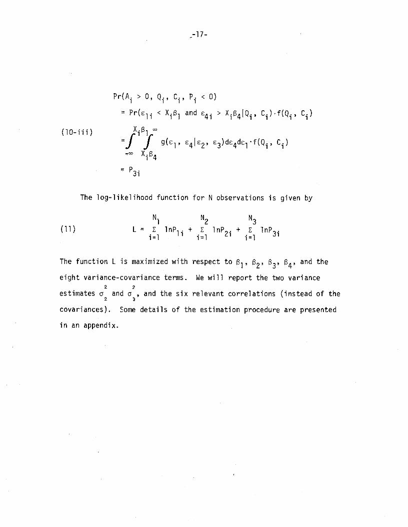
The log-likelihood function for N observations is given by
N1 N2 N3(11) L =
lnP1.+ E lnP2. + lnP.
i=l1 i=l 1 i=1 1
The function L is maximized with respect to l' 2' and the
eight variance-covariance terms. We will report the two variance2 2
estimates a and a , and the six relevant correlations (instead of the2 3
covariances). Some details of the estimation procedure are presented
in an appendix.

-18-
II. The Data
We have based our estimates on data obtained from the National
Longitudinal Study of the High School Class of 1972. During the Spring
of 1972, approximately 23,000 high school seniors were surveyed. The
data collected included information on each student's family back-
ground, high school performance, and a host of other student character-
istics. The students also took a battery of six aptitude tests
developed by the Educational Testing Service (ETS). Three fol1ow-u
surveys were used to obtain information on post-secondary school and
work decisions as well as other related data. We have based our esti-
mates on a random sample of ,726 of the total sample.
We have confined our attention to four-year colleges and univer-
sities. For example, the probability of attendance refers to the
probability of attendance at a four-year college; some of those who
didn't go to four-year schools went to two-year or vocational schools.
Our analysis is based on several groups of variables. The first
group includes variables that describe the individual's academic
aptitude and high school performance, as well as non-academic achieve-
ment in high school.
The Scholastic Aptitude Test (SAT) score of an individual is
presumed to have a substantial effect on his post-secondary school
preferences and on available alternatives. Although SAT scores are
recorded for many students in our sample, not all of them took the SAT
test. Many took no college admissions tests at all, while others took
the American College Testing Program (ACT) test. Our method of analysis
requires that we have an academic ability measure for all persons in the
sample, not only for those who took the SAT test--undoubtedly for most

-19—
because they planned to apply to some school. For this reason, we have
used an "SAT" score predicted on the basis of the ETS test scores that
are available for each person in our sample.
High school class rank is also presumed not only to influence
students' preferences for college but to measure individual attributes
related to college persistence as well. An individual's class rank
is determined not only by his ability, but also by the ability of others
in his high school. We do not have a definitive measure of high school
quality, but have tried to control for it in part by including in our
analysis the percent of students from an individual's high school who
go to college. Finally, we have used two measures of non-academic
achievement in high school: leadership in student government and
athletic achievement.
The second group of variables is intended to measure an individ-
ual 's socioeconomic background; it includes family income and parents'
education. Race is also included, with the effect of race allowed to
interact with geographic region--South versus non-South.
The third group includes two measures of local labor market con-
ditions: a local wage rate and a local unemployment rate. These
variables enter the attendance equation only. The analysis also
includes an indicator of sex, and an indicator of rural versus city
or urban high school location.

—20-
The variables are defined as follows:
SAT Score: predicted SAT scores based on 5 of the 6 ETS tests
administered to the National Longitudinal Study sample.
College SAT: the average of the SAT scores of freshman students
at the college. We often refer to this as college quality.1
College Cost: tuition and living expenses, minus grant aid to
the student.
High School Class Rank: the percentile rank of a person in the
person's high school, based on course grades.
Leader: one if the person was a
"leader" in high school student government nd zero otherwise.
High School Athlete: one if the student was a "leader" in high
school athletics and zero otherwise.
Percent of High School Class Going to Colig: the percent of
students from an individual 's high school who go to colleges.
Parents' Income: family income as reported by the youth respondent.
Education of Mother (Father) less than High School: one if the indi-
vidual's mother (father) had less than a high school education and zero
otherwise.
Education of Mother (Father) College Degree or More: one if the
individual's mother (father) had a college degree or more education, and
zero otherwise. The excluded category is a high school degree but less
than a college degree.
1. Solmon [1975] discusses several alternative measures of collegequality and expresses a preference for SAT scores over survey measuressuch as the Gourman ratings. See also Astin and Henson [1977].

—21—
Siblings: the number of non-adult dependents of the individual's
parents.
Black in the South: one if the person is black and went to high
school in the South.
Black in the Non-South: defined analogously to black in the South.
White in the South: defined analogously to black in the South.
The excluded category is white in the non—South.
Local Wage Rate: average 1972 wage of manufacturing workers in the
SMSA of the individual 's high school, or if not available, the state average.
Local Unemployment Rate: SMSA 1972 unemployment rate (or state rate
where not available).
Male: one if the individual is male and zero if female.
Rural: one if the individual went to high school in a rural area
and zero otherwise.
Parents' Income Missing: one if parents' income was not reported and
zero otherwise.
Means and standard deviation of the variables are shown in Appendix
Table 1.
1. South is assumed to include the following states: Alabama,
Arkansas, Delaware, Washington, D.C., Florida, Georgia, Kentucky,Louisiana, Maryland, Mississippi, North Carolina, South Carolina,Virginia, Idest Virginia.

—22—
III. Results
We shall present first the parameter estimates and discuss the im-
plied partial effects of specified changes in each of the right-hand
variables. Then we shall present more detailed simulations based on the
parameter estimates--the first to describe the effect of changes in SAT
scores and high school class rank and the second to describe the effect
of changes in parents' income and education. The quantitative implica-
tions of self-selection are presented next. Finally, predictions based
on SAT scores and class rank only are discussed, with emphasis on their
relationship to current criticism of SAT scores.
A. The Parameter Estimates and Normalized Partial Effects ofIndividual Variables
The parameter estimates and their asymptotic standard errors are
shown in Table 1. We shall not present standard error estimates
for the simulations, but we emphasize that the major coefficients in
the model are measured with considerable precision, as shown by the
standard errors in Table 1. For example, many of the implied t -
statistics on the SAT and class rank variables are 10 or more. To
evaluate the partial effects of each of the variables, in Table 2
are shown the predicted shifts in each of the four outcomes due to
specified changes in each of the right-hand variables.
The correlations among the unmeasured determinants of each of
the outcomes are shown at the bottom of Table 1. It is clear from these
correlation estimates that unmeasured attributes that increase an
individual's propensity to attend college are strongly related to the
unmeasured attributes that determine the cost and the quality of the

-23-
college he would choose, were he to attend; the relevant correlations
are .94 and .45 respectively. Given measured attributes, the more
value an individual attaches to college attendance, the more he is
willing to pay for a college education and the more likely he is to
go to a higher quality school. Of course, both the average SAT score
of entering students and the cost of attendance may be measures of
college quality. (It can also be seen that the unmeasured determinants
of college quality and college cost are positively related as casual
observation would suggest.)
The results in Table 2 show the effects of the specified changes
in each of the variables, assuming that all other variables are held
constant at their respective population means. If the variable is
continuous, the outcome with this variable one standard deviation above
its mean is compared with the outcome with the variable one standard
deviation below its mean. For example, holding other variables at their
sample means, a person with an SAT score one standard deviation above
the mean for all persons is estimated to have a probability of college
attendance .234 higher than a person with an SAT score one standard
deviation below the mean. Evaluated at the mean of all the right-hand
variables, the expected attendance probability is .21, college quality
is 908, college cost is -$314, and the persistence probability is .47.
By these measures SAT scores and high school class rank are of
approximately equal importance in determining college attendance, college
quality, and college cost. But the relationship of class rank to per-
sistence is over three times as great as the relationship to persistence
of SAT scores. That is, once persons enter the schools optimal for

-24—
them, given their measured characteristics, high school ciass rank is
a stronger indicator of persistence than are SAT scores, although both
are statistically significant. This result is not surprising if it is
assumed that given academic ability or achievement as reflected in
SAT scores, class rank reflects in part differences in individual
effort or desire to perform well. Recall that the model also controls
for high school "quality," to the extent that it is measured by the
proportion of students from an individual's high school who go to
college. It can also be seen in Table 2 that holding constant other
variables, including SAT score and high school class rank, persons
from "better" high schools are considerably more likely to persist
in college.
It might be expected that given an indication of how well a student
performed academically as well as an indication of the abilities of
those with whom he was competing, the additional information that the SAT
score provides would be limited. The former two measures provide obser-
vations on the sort of performance that SAT scores are intended to predict,
but in high school instead of college. Because together they provide an
observation that is similar to what the SAT score is intended to predict,
it should not be surprising that they are better predictors of subsequent
but similar student performance than SAT scores are. We will see below
that if predictions are based solely on SAT scores and class rank, the
importance of knowing SAT scores is considerably greater.
The difference in the probability of college attendance, as well
as college quality and cost, associated with college educated parents

—25—
Table 1. Parameter Estimates (and Asymptotic StandardErrors), by Equation.
R
High School Class Rank÷ 100
Proportion of HighSchool Class Going toCollege
Student
High School Athlete
Parents' Income
Education of MotherLess than High School
Education of MotherCollege Degree or More
Education of FatherLess than High School
Education of FatherCollege Degree or More
Siblings
Black in the South
Black in the Non-South
White in the South
Rural High School
0.809
(0.120)
0.370
(0.061)
0.220
(0.049)
0.138
(0.063)
-0.244
(0.055)
-0.026
(0.012)
0.749
(0.105)
0.925
(0.100)
-0.016
(0.045)
CollegeQuality
0.060 0.691
(0.015) (0.135)
0.027 0.286(0.007) (0.067)
0.019 0.401
(0.006) (0.055)
0.014 0.172(0.007) (0.066)
-0.008 -0.221
(0.007) (0.068)
0.033 0.655(0.012) (0.116)
-0.013 0.055(0.006) (0.052)
1.025
(0.226)
0.140
(0.105)
0.108
(0.094)
-0.072
(0.106)
0.006
(0.196)
-0.027(0.080)
Variable
SAT Score 1000
I
Probabilityof Attendance
College Probability ofCost Persistence
2.233 0.225 1.700(0.160) (0.021) (0.193)
0.786
(0.305)
1.454 0.142 1.093(0.106) (0.016) (0.132)
1.613
High SchoolLeader
0.246
(0.072)
0.023 0.154 -0.042(0.008) (0.082) (0.106)
-0.129(0.056)
- -0.010(0.008)
-0.158
(0.068)
0. 357
(0.085)
0.029
(0.114)
0.254
(0.057)0.025 0.242(0.007)
0.140(0.062)
-0.002 -0.028 -0.012(0.002) (0.014) (0.023)
—0.127 0.594 0.510(0.011) (0.147) (0.181)
0.038 -0.033 -0.111(0.055) (0.007) (0.061)
-0.162
(0.086)

-26-R
Table 1. Parameter Estimates (and Asymptotic Standard Errors),
by Equation (continued).
VariableProbability College College Probability of
of Attendance Quality Cost Persistence
Local Wage -0.136
(0.031)
Local Unemployment Rate 0.000
(0.008)
Male 0.193 0.021 0.132 0.032
(0.044) (0.005) (0.051) (0.079)
Parents' Income Missing 0.231 0.025 0.521 0.415
(0.080) (0.010) (0.095) (0.144)
Constant -3.680 0.601 -3.081 -2.509
(0.199) (0.032) (0.234) (0.458)
Correlation Matrix
Attendance 1.000
College Quality 0.451 1.000
(0.056)
College Cost 0.935 0.389 1.000
(0.011) (0.046)
Persistence 0.155 0.047 0.135 1.000
(0.099) (0.048) (0.074)
Standard
College
Error of
Quality
0.098
(0.005)
Total
Number
Sample
Attending
5726
1622
Standard Error of 1.122Persisting 1155
College Cost (a3) (0.055) Number
Log—Likelihood Value -532.1
a. College quality for purposes of estimation is in 1000's, college cost is
in 1000's, student SAT is in 1000's, and parents' income is in 10,000's.

-27- R
Table 2. Effects of Two Standard Deviation
Changes in Variables, by Equationand Category
SAT Score 1 S.D. Abovethe Mean Versus 1 S.D.Below the Mean
High School Class Rank,1 S.D. Above the MeanVersus 1 S.D. Belowthe Mean
High School StudentLeader Versus Not
High School AthleteVersus Not
Percent of High School
Class Going to College,1 S.D. Above the MeanVersus 1 S.D. Below theMean
Parents' Income, 1 S.D.Above the Mean Versus 1S.D. Below the Mean
Education of Mother andFather College Degree orMore Versus Education ofMother and Father LessThan High School
Number of Siblings, 1S.D. Above the Mean,Versus 1 S.D. Below theMean
.234 81.0
.231 77.8
.078 23.1
.121 27.2
611.8 .112
597.3 .340
154.4 -.017
285.7 .056
.153
VariableofProbability
AttendanceCollegeQuality
CollegeCost
Probability ofPersistence
.090 22.7 260.2
.070 20.5 430.8 .152
.233 56.9 791.9 .116
-.005 -.007 -93.8 -.017

-28-R
Table 2. Effects of Two Standard Deviation and CategoryChanges in Variables, by Equation (continued).
VariableProof
babilityAttendance
CollegeQuality
CollegeCost
Probability ofPersistence
Black in the South .265 -127.1 594.4 .198
Versus White in theNon-South
White in the South .011 -33.4 -110.8 -.064
Versus White in theNon-South
Black in the Non-South .336 32.7 654.5 .002
Versus White in theNon-South
Male Versus Female .057 20.7 132.3 .013
Rural Versus Non-Rural -.005 -13.4 55.2 -.011
High School
Local Wage, 1 S.D. Above -.047
the Mean Versus 1 S.D.Below the Mean
Local Unemployment Rate, .000
1 S.D. Above the MeanVersus 1 S.D. Below theMean

-29-
versus parents without high school degrees is quantitatively similar
to the effect of a two-standard deviation change in class rank and SAT
scores. A two-standard deviation change in parents' income on the
other hand has a relatively small effect on college attendance and type
of college, but has a greater effect on persistence than the change
(just described) in parents' education. Parents' education is apparently
much more important than income in determining preferences for education,
but after entering college, income is relatively more important than
parents' education in determining persistence.
Black youth are more likely than white youth, given other attributes,
to go to college. In the South, the probability that black youth attend
is .25 higher than the probability for white youth with the same attributes.
In the non-South, the probability is .34 higher for black youth. While
black youth in the South go to colleges with average SAT scores about 94
points lower than white youth in the South, the persistence rate of black
youth is about .26 higher than the rate for white youth. The persistence
rate of black youth in the South is about .20 higher than the rate of
black youth in the non-South. While black youth in the South go to
colleges with average SAT scores about 160 points lower than black youth
in the North, their probability of persistence is about .20 higher than
the persistence probability of black youth in the non-South. In the non-South,
black youth go to colleges with student SAT scores that average a bit
higher than those of schools attended by white youth, given academic
and socioeconomic characteristics.
That black youth are more likely than white youth to go to college,
given comparable academic and family background attributes, may reflect
-30-
the relatively greater returns to higher education for blacks, as found
for example by Freeman [1976, 1978]. The atmosphere created by emphasis
on affirmative action may also have encouraged more black youth to go
to college. The average SAT scores of students in most predominantly black
schools (largely in the South) are low relative to the least selective
schools in the non-South. Thus some students in the South may be be attracted
to a college alternative that doesn't exist in other regions of the country.
In addition, some black youth who go to four-year colleges in the South
might be more likely to go to two-year colleges if they lived in the non-
South.
The greater returns to education for black youth are consistent also
with the finding that given other attributes black youth pay more
to go to college than white youth. The estimated effect of the race-region
variables on cost assumes of course that other attributes--in particular
SAT scores--are held constant. When these attributes are not held constant
we find the average college cost for blacks is lower than for whites in
both the South and the non-South, while in both regions the average of
black SAT scores is about 170 points lower than the white average. These
and other means of selected variables by race and region are shown in
Appendix Table 2.

—31—
B. The Probability of Attendance versus the Probability of Dropping Out
In the next section we shall present simulated partial effects of
selected variables on each of the four outcomes. These simulations,
however, don1t provide an overall indication of the relationship between
attendance and persistence. To provide such a summary we have presented
in Figure 1 a graph of the probability of attendance versus the probability
of dropping out. To relate the probability of dropping out more purely
to student decisions, we have also graphed this probability against the
probability of application, taken from Venti and Wise [1980]. That is,
for each individual in our sample, we have predicted attendance (and
application) and dropout probabilities. Then, for each attendance (or
application) interval, we have calculated the average dropout probability.
These predictions are thus based on all measured determinants of the
outcomes.
The figure indicates that persons who are unlikely to attend college,
on average would be very likely to drop out were they to attend. The
same pertains to those who are unlikely to apply to any college. On the
other hand, persons who are likely to apply, and attend, are very unlikely
to drop out. In this sense, student application and attendance decisions
seem to be quite consistent with persistence outcomes and more generally with
rational educational investment decisions. To the extent that the expected
benefit from college is determined by whether a degree is obtained, persons
with high expected benefit are likely to go while those with low expected
benefit areunlikely to go.

4-,
•10C
0>4-,F
.00S.-
0 0.1 0.2 0.3
ProbabilityAttendance,
0.8 0.9 10
of
Application
S.
-32-
Figure 1. Probability of Attendance and Application VersusProbability of Dropping Out.
1.0
0.9
0.8
0.7
0.6
0.5
0.4-
0.3
0.2
0.1
\
Attendance
icat ion
0.4 0.5 0.6 0.7
\

—33-
C. Simulated Effects of Selected Variables
1. SAT Scores and Class Rank.
Estimated probabilities of attendance and dropping out, together
with estimated college quality and cost, are presented in Table 3 for
selected SAT and class rank values. Differences among the entries in
the table represent estimated partial effects of SAT and class rank, with
other variables in the model assigned their population means.
Persons with SAT scores and class ranks that make them unlikely
college entrants would have a high probability of dropping out were
they to go to college. For example, persons with SAT scores of 900 or
lower and in the bottom half of their high school classes have at most
a .24 probability of going to college. If persons in this group were
to attend, their dropout probabilities would be very high, at least
.53 and ranging up to .88 for those with the lowest test scores and
poorest academic records. On the other hand, persons with scores and
class rank that yield high estimated attendance probabilities are much
less likely to drop out than those with low scores and class rank.
While attendance probabilities range from .01 to .82, corresponding
dropout probabilities range from .88 to .15.
We see also from Table 3 that if persons were to choose among
college possibilities, the qualities of the schools they would choose
would vary with their own academic abilities, as casual observation would
suggest. Recall that estimated college quality and college cost repre-
sent the characteristics of the school a person with given attributes—-
randomly selected from the population--would choose, were he to choose

34R
Table 3. Simulated Effects of SAT and High School Class Rankon Attendance, College Quality and Cost and on the
Probability of Dropping Out
SATClass Rank (Percentile)
0 25 50 75 100
Probability of Attendance
500 .01 .03 .06 .11 .19
700 .03 .07 .13 .22 .34
900 .08 .15 .24 .37 .51
1100 .16 .27 .40 .55 .68
1300 .30 .43 .58 .71 .82
College Quality
500 755 791 826 862 898
700 800 836 871 907 943
900 845 881 916 952 988
lipO 890 926 961 997 1033
1300 935 971 1006 1042 1076
College Cost
500 —1372 —1099 -825 -552 -279
700 -1032 -759 -486 -212 61
900 -692 -419 -146 128 401
1100 -352 -79 194 468 741
1300. -12 261 534 807 1081
Probability of Dropping Out
500 .88 .79 .65 .49 .34
700. .85 .74 .59 .43 .28
900 .81 .68 .53 .37 .23
1100 .76 .62 .47 .31 .19
1300 .71 .56 .40 .26 .15

-35-
among colleges. Thus it is also not surprising that persons who are
unlikely to find school attractive would pay little to attend. Indeed
these estimates indicate that for many persons the optimal college would
be one that they were paid to attend; the estimated cost is negative.
"Desired' college cost is not constrained to be positive.1
As mentioned above, the partial effects--after controlling for a
measure of the academic level of an individual's high school, as well as
socioeconomic background and other variables--show that the effect on
persistence of high school class rank is much greater than the effect of
SAT scores on persistence. If the percent of students from a person's
high school who are college bound is not controlled for, however, the
corresponding variation in dropout probabilities by SAT score is much
greater than is shown in Table 3. (Such estimates are presented below.)
The attendance and dropout probabilities in Table 3 may be integrated
with the application and admission probabilities from our earlier paper
(Venti and Wise [1980]), based on a model with the same variables used
in this paper. These results are shown in Table 4.
Based on the application and admission probabilities shown in
Table 4, we concluded in our earlier paper that SAT scores were related
much more to individual application than to college admission decisions.
Most persons would have a high probability of admission were they to
apply to a college of average quality. It is clear also from Table 4
1. Because unmeasured determinants of attendance are positivelyrelated to quality, cost, and persistence, the conditional quality andcost estimates are higher than the unconditional ones, and the dropoutprobabilities are lower. This idea is pursued further in Section D below.

-36-
Table 4 Simulated Application, Admission,Attendance, and Dropout ProbabiUtieSafor Selected SAT and Class Rank Values
SAT
Class Rank (Percentile)
0 25 50 75 100
Probability of Application
500 .03 .06 .11 .19 .30
700 .07 .14 .23 .35 .49
900 .17 .27 .40 .54 .68
1100 .31 .45 .59 .72 .83
1300 .50 .64 .76 .86 .92
Probability of Admissionb
500 .52 .63 .74 .82 .89
700 .64 .74 .82 .39 .93
900 .74 .82 .89 .93 .96
1100 .83 .89 .94 .96 .98
1300 .89 .94 .96 .98 .99
Probability of Attendance
500 .01 .03 .06 .11 .19
700 .03 .07 .13 .22 .34
900 .08 .15 .24 .37 .51
1100 .16 .27 .40 .55 .68
1300 .30 .43 .58 .71 .82
Probability of Dropping Out
500 .88 .79 .65 .49 .34
700 .85 .74 .59 .43 .28
900 .81 .68 .53 .37 .23
1100 .76 .62 .47 .31 .19
1300 .71 .56 .40 .26 .15
a. The probability of application and the probability of admission
from Venti and Wise [1980].
b. At a college of average quality (with an average SAT of 1012).
R

-37-
that some persons with a high estimated probability of admission have
a low estimated probability of attendance. In particular, this is true
of persons whose SAT scores, and/or class ranks are below the sample
averages.1 This result also supports the finding that to the extent
that SAT scores determine college attendance, their effect is more by
way of individual than by way of college admission decisions.
And whether we consider the individual application decision or the
attendance decision outcome--that incorporates both student and college deci-
sions—-the relationship between test scores and these decisions seems
supported by the dropout probabilities. To the extent that test scores
affect student and college decisions, in the aggregate, they tend to be
consistent with the dropout probabilities. We will pursue this point
in Section E.
2. Income and Parents' Education.
Simulated attendance and dropout probabilities together with college
quality and cost for selected levels of parents' education and family
income are shown in Table 5. Again, they are unconditional estimates--
representing the predicted choices of a person with the given attributes
selected from the pooulation: colleae charartrictirs and dropout
probabilities conditional on attendance differ from these, as shown in
Section D below.
1. In part, these estimates pertain to SAT and class rank combi-nations that would be unlikely to be observed empirically. For example,because SAT and class rank are positively correlated, very high SAT andvery low class rank is uncomon.

-38-
Table 5. Simulated Effects of Parents' Income and Educationon Attendance, College Quality and Cost, and onthe Probability of Dropping Out.
Parents'Education
Parents' Income
$6,000 $9,000 $12,000 $15,000 $18,000
Probability of Attendance
Less than HighSchool
.11 .13 .14 .15 .17
College DegreeMore
or .33 .35 .38 .40 .43
College Quality
Less Than HighSchool
879 885 890 896 902
College Degree or 936 941 947 953 959
College Cost
Less Than HighSchool
-747 -627 -507 -387 -267
College DegreeMore
or 45 165 285 405 525
Probability of Dropping Out
Less Than HighSchool
.62 .57 .53 .49 .45
College DegreeMore
or .50 .46 .42 .38 .34
R
-39-
Relative to parents' education, parents' income appears to affect
dropout probabilities much more than attendance or college quality or
college cost. Apparently persons whose parents earn less are substantially
more likely to drop out of college for monetary reasons than persons
from wealthier families, if family income is interprested strictly as a
determinant of individual budget constraints. This observation is con-
firmed by the estimated effects of two standard deviation shifts reported
in Table 2. Indeed parents' income hasconsiderably less effect than
SAT scores except in the determination of dropping out. Parents' educa-
tion, on the other hand, is by thesecomparisons relatively less important
in the determination of dropping out than in the determination of atten-
dance and college characteristics. Judging by the evidence in Table 2,
however, the three measures of individual academicability--SAT scores,
the percent of the individual's high schoolclass who go to college, and
high school class rank—-taken together are much more important than family
income in the determination of persistence.Nonetheless, our results
suggest that if educational attainment were not to be related to family
income, for example, low family income would have to be offset by external
funds, even if income itself were not a major determinant of college
attendance.
1. Recall that we have used net college cost, subtracting aidfrom college tuition plus living cost. Holding other determinantsconstant, persons from poorer families obtain more aid than personsfrom wealthier families, although in 1972 academic performance was animportant determinant of aid. In subsequent years after the introduc-tion of the federal Basic Equal Opportunity Grant program, relativelymore aid was allocated in inverse relation to family income. (SeeFuller, Manski, and Wise E1980a, 1980b].)

-40-
D. The Importance of Self-Select1fl
The foregoing results highlight the very substantial relationship
between measured individual attributes on the one hand and college
selection and persistence on the other. The effect of measured attributes
on outcomes, however, represents only one of the components of self-selec-
tion. The other is the effect of unmeasured individual attributes which may
be expected to have comparable effects on self-selection. In particular
we proposed above that given measuredattributes, individuals who elect
to go to school are likely to be disproportionatelythose whose relative
opportunities will be most enhanced by college or who most enjoy school,
etc., and who are the most likely to succeed in college. The estimated
correlations among the disturbance terms reported in Table 1 support
this proposition. The correlations may be interpreted as an indication
of self-selection bias.1
To provide a better measure of the importance of this form of self-
selection, we have estimated the difference in college quality, college
cost, and the probability of dropping out, conditional on attendance
versus conditional on non-attendance. The results evaluated at the
population means of all variables are as follows:2
Conditional on Conditional on
Attendance Non-Attendance Difference
(1) (2) (l)—(2)
College Quality 966 893 73
College Cost 1188 -720 1908
Probability of 0.45 0.55 -0.11
Dropping Out
1. See Hausmarl and Wise [1979], for example.
2. The probabilities have been rounded to the nearest hundredth.

-4l-
Given personal attributes, persons who elect not to go to college, if
they were to attend, would choose schools of lower quality than the
schools selected by persons with the same attributes who go to college.
Also, among persons with the same attributes, those who don't go would
have a higher probability of dropping out than persons who are observed
to go. Possibly most noticeable is the very large difference between the
average cost of schools selected by those who attend versus the cost
"desired" by students who don't attend. On average, students who attend
are prepared to pay much more for college than those who don't attend.1
E. The Information Content of SAT Scores and Class Rankarid Implications for Test 'Validity."
The simulations above are based on a model that we believe incor-
porates measures of the major determinants of college-going decisions,
namely, it incorporates both academic and family socioeconomic variables.
Measures of academic ability and past performance are assumed to be
reflected in SAT scores, high school class rank, and the proportion of a
person's high school classmates who go to college. Thus all of the
above estimates are of partial effects after controlling for other
variables. In particular, unreported estimates suggest that when the
percent of an individual's high school classmates who go to college is
1. Mechanically, these effects are due to the size of the Millsratio for the different values of X. For example, the expected value ofcost given attendance is
+p13a3(q(X1)/[x1]) ,
where X3 is shown in Table 3, p13 = .935 and a3 = 1122; is the unit
normal density function and is the corresponding distribution function.

-42-
added to the model, the relationship between high school class rank
and dropping out of college becomes larger and the partial relationship
between SAT score and dropping out smaller. The percent of high school
classmates who go to college appears to be an alternative measure of
the academic ability of the individual; or class rank relative to SAT
score means more if we have an indication of the abilities of the students
against whom he was competing.
But much of the recent discussion on the subject is motivated by
claims that the predictive "validity of the tests is low, in particular
relative to high school class rank. To address these claims, we have
estimated our model using only SAT scores and high school class rank,
together with the three race-region variables. Simulations analogous
to those in Table 4, but based on this limited predictive model, are
shown in Table 6. (Parameter estimates analogous to those in Table 1
but based on the simplified model, together with simulations analogous
to those in Table 3, are shown in Appendix Tables 3 and 4 respectively.)
It is clear from the bottom section of the table that given high
school class rank, substantial predictive information is contained in
SAT scores. The change in the dropout probability associated with a
200 point change in the SAT score is about the same as the change in
the dropout probability associated with a 25 point change in class rank.
For example, begin with a person at the 50th percentile in his high
school class and with an SAT of 900. If the person instead were at the
75th percentile in class rank the estimated dropout probability would be
.11 lower; similarly if instead the person had an SAT score of 1100,

43 R
Table 6 Simulated Application, Admission, Attendance,and Dropout Probabilities, for Selected SAT
aand Class Rank Values, Based on Simplified Model
SATClass Rank (Percentile)
0 25 50 75 100
Probability of Application
500 .02 .04 .07 .11 .17
700 .09 .14 .21 .29 .39
900 .25 .34 .44 .54 .64
1100 .49 .60 .69 .78 .85
1300 .74 .82 .88 .92
Probability of Admissionb
.95
500 .45 .59 .71 .81 .89
700 .56 .69 .79 .88 .93
900 .66 .78 .86 .92 .96
1100 .76 .85 .91 .96 .98
1300 .83 .90 .95 .98 .99
Probability of Attendance
500 .01 .02 .03 .06 .10
700 .04 .07 .12 .18 .25
900 .14 .21 .29 .38 .49
1100 .33 .43 .53 .63 .73
1300 .58 .68 .76 .83 .89
Probability of Dropping Out
500 .86 .79 .70 .60 .49
700 .78 .69 .59 .48 .37
900 .68 .58 .47 .36 .26
1100 .57 .46 .35 .25 .17
1300 .44 .34 .24 .16 .10
a. Based on a model that includes only SAT and class rank togetherwith the race-region variables.
b. At a college of average quality (average SAT of 1012).

-44-
The dropout probability would be .12 lower.1
Comparisons based on high school class rank and SAT score are
important because these are the measures that are most often considered
in evaluation or criticism of the predictive validity of test scores,
or the information content of the scores. The criticism, however, is
often justified on the basis of the limited increase in the multiple
correlation between college grades on the one hand, and high school
class rank and SAT scores on the other, over the simrle correlation2
between college grades and high school class rank. Even though the
relatively high correlation between SAT scores and high school class
rank (.50 in our sample) means that expected dropout probabilities can
be predicted well with only high school class rank, given class rank the
difference in expected dropout probabilities varies greatly with SAT
scores. This means that although on average colleges could predict
reasonably well on the basis of class rank alone, these predictions
would be far from expected dropout probabilities in some instances.
In particular, individuals with SAT scores very different from the
expected SAT score given class rank would be either substantially disad-
1. A 200 point change in SAT scores and a 25 point change
in class rank are both roughly equivalent to one standard deviation.
Calculations based on an exact one standard deviation change yield
a .11 change in the dropout probability for each of them.
2. The validity coefficient is the binary or multiple correla-
tion between the criterion variable and one or more predictor vari-
ables. A recent survey of over 800 studies of college grades versus
SAT scores and high school performance found validitycoefficients of
about 0.52 for high school performance, 0.41 for SAT score, and 0.58
for both predictors together. See Ford and Campos [1977].

-45-
vantaged or substantially advantaged if admissions were based on class
rank alone.
It is also informative to compare the estimated weights associated
with the two measures in individual decisions versus college admission
decisions. According to our formulation of the problem the estimated
coefficients in the student attendance equation represent the
ship between the associated variables and the individual's evaluation
of opportunities with education at the school he could attend versus
opportunities without college. A similar interpretation can be given to
estimated coefficients in the application and dropout equations. In the
admission equation, the coefficients may be interpreted as the weights
that colleges and universities assign to these measures in determining
an individual's academic potential.1
For each estimated relationship we have calculated the ratio of
the SAT to the class rank coefficient; that is, the number of class rank
percentile points that is equivalent to 10 SAT score points. The results
are as follows:2
Probability of Application 3.14
College Quality (Application) 3.94
College Quality (Attendance) 3.10
1. See Venti and Wise [1980].
2. The ratios in the probability of application, college quality(application), and the probability of admission equations are taken from
equations analogous to those in Venti and Wise [1980], but based only onSAT scores and class rank together with the race-region variables.

-46-
College Cost (Attendance) 3.78
Probability of Attendance 3.05
Probability of Admission 1.02
Probability of Persistence 1.38
In the light of recent criticism of the use of SAT scores in admissions,
it is striking that the class rank percentile point equivalent of 10
SAT points is a bit less in admissions than it is in rredicting
persistence. Thus should persistence be the criterion for admission,
colleges and universities on average may if anything assign a somewhat
lower weight to SAT scores versus high school performance than persistence
predictions suggest.
Note also that relative to class rank, SAT scores bear a much
greater relationship to the values that individuals assign to oppor-
tunities with and without college than they do to the "average" univer-
sity's evaluation for admission purposes. The importance of the individual
attributes reflected in SAT scores shows up not only in individual applica-
tion decisions but in college quality and cost decisions as well. On average
these (by and large) individual decisions are also much more strongly
related to test scores than college admission decisions are. The same may
be said for ultimate attendance decisions, largely individual choices but
affected in part by college admission decisions.
Apparently, the relationship between test scores and what individuals
think they can get out of school is much more pronounced than colleges
and universities--in effect society's--evaluation of the opportunity
that should be available to them should they want to enter college,

-47-
indeed much greater than the realtionship between test scores and
academic success, measured by observed persistence. Individuals are
likely to evaluate schooling opportunities not only in terms of persis-
tence but in terms of human capital development while in school (and
subsequent earning gains) and simply enjoyment of schooling as well.1
Both would suggest that student schooling decisions are determined more
by academic ability than university admission decisions are. Individuals
not only weight academic ability highly in deciding whether to go to
college at all, but are also willing to pay more for a college education
if they have greater academic ability. And persons with greater academic
ability are also likely to choose a more competitive and higher quality
college. Both are consistent with rational individual human capital
decisions. Simply put, the results are consistent with the hypothesis that
the net returns to education are low for persons with low academic ability
or interest. Colleges on the other hand don't insist that every entrant
do well; neither do they insist that every entrant like school. Individuals
whose lives are personally affected by such things, apparently are much
more inclined to take them into account in making their decisions.
Apparently, the provision of individual college opportunities in general
is considerably more in the hands of individuals than at the behest of
institutions, and apparently the individual decisions are strongly related
1. One explanation may be complementarily between ability (asmeasured by test scores) and schooling in the determination of earnings.The value of a college degree may be more for students higher in theattributes measured by test scores. These attributes may also be moreclosely related to the consumption aspects of schooling.

-48-
to the attributes reflected in SAT scores.
We note also that the relative weight of SAT scores is much lower
in persistence than in the other individual decisions (supposing that
persistence is largely an individual and not an institutional choice).
SAT scores of course provide a comparison of individual attributes with
those of a much broader population than is provided by class rank which
compares an individual only with his high school classmates. Since in
making post-secondary schooling decisions an individual is likely to
think of his attributes relative to those of a group much broader than
his high school classmates, it is not surprising that the attributes
reflected in SAT scores should weight relatively more heavily than high
school class rank. On the other hand, once individuals have allocated
themselves to college versus no college and among colleges, in large
part according to the attributes reflected in SAT scores, it is also
not surprising that given this allocation, class rank should weigh
relatively more heavily in determining persistence than in determining
college attendance and college type.
We emphasize that the calculations in this section derive from
predictions based on SAT scores and high school class rank only. As we
have already mentioned, relative to class rank the partial effect of
SAT scores on dropping out is considerably less in the more behavioral
model (Table 3 for example) than in the simplified specification. In
large part the difference results from the inclusion in the behavioral
specification of the percent of an individual's high school class who to
to college: Apparently though, SAT scores in the simple model also pick

-49-
up to some extent individual attributescontributing to success in
college but that should be ascribed to family socioeconomic background
rather than academic ability. Inparticular, family income affects
persistence and its effect is apparently pickedup in part by SAT scores
when income is not included in the model. In any case, it is clear that
the additional predictive information containedin SAT scores, given high
school class rank, would be less if family background variables were
also used to predict dropout probabilities. Such predictions used in
admission decisions, however, would surely be ethically inappropriate
and indeed legally proscribed.

-50-
IV. Concluding Comments and Discussion
Our earlier work demonstrated that a very large proportion of
college applicants gain admission to their 'first-choice" school. The
self-selection by students of colleges and universities is striking. In
particular, SAT scores are more closely related to the student than to
university choice. These findings together with the results reported in
this paper suggest that test scores (or the attributes reflected in them)
are at least as important in student decisions as in admission decisions.
It is not only the university that would like to compare one student to
another, but the student who would like to judge his academic abilities
relative to other students. Our findings suggest that SAT scores are likely
to contribute in substantial measure to rational college attendance
decisions and indeed may aid student choice more than university choice.
In a statistical sense, this self-selection can be thought of in two
components. One is the part that is explained by observed individual
characteristics. The other is associated with unobserved characteristics
and is reflected in positive correlations between the random determinants
of college attendance and the random determinants of persistence in
college (as well as the random determinants of college quality and college
cost). For example, an individual with average attributes who attends
college will drop out with estimated probability .45, while an individual
who is observed not to attend would have a .55 probability of dropping out.
This is analogous to the self-selection component hypothesized by Willis
and Rosen [1979] with respect to college attendance and earnings with and
without a college degree.

-51-
College attendance and non-attendance decisions are consistent
with the strong relationship between the likelihood of attendance and
the likelihood of benefitting from college by obtaining a degree. Persons
who are unlikely to attend are very likely to drop out without a degree
should they attend and persons who are likely to attend are unlikely to
drop out. In addition, the relationship between SAT scores and high
school class rank and the probability of college attendance is strongly
mirrored by an opposite relationship between these measures and the
probability of dropping out of college, if a college should be attended.
Our results also confirm that the quality of school persons attend--largely
by choice--is strongly related to their aptitude and past performance in
high school. This finding is in accord with casual observation, but it is
also consistent with evidence based on choice models of selection among
schools to which persons have been admitted.1 Possibly less obvious,
but consistent with economic reasoning, is the result that persons who
are unlikely to succeed in school, if choosing among colleges would
not only select low quality schools but low cost schools as well. Indeed
for many, the preferred school would ba one that individuals were paid to
attend. Persons who are unlikely to succeed in school on average would
not be as inclined to pay a lot for the privilege.
To the extent that colleges base admissions decisions on test scores,
their selection procedures distinguish persons according to expected
probability of success. Indeed the relative weight assigned to SAT scores
1. See Radner and Miller [1975], Kohn, Manski, and Mundel [1976],and Fuller, Manski, and Wise [1980a].

—52-
versus high school class rank by college admissions officers is
s'mewhat less than the relative weight of SAT scores in the prediction
of the probability of college persistence. (This is not to say of course
that test scores necessarily explain a great deal of the variation in
academic performance.)
Our findings are inconsistent with the implications of much of the
recent discussion and criticism of test scores. Predictions based on SAT
scores and high school class rank yield estimates that distinguish rather
dramatically the school preference and college success probabilities of
high school graduates. Our previous research indicated that the relation-
ship between these measures and college attendance outcomes was due much
more to their relationship to individual application decisions than to
their effect on college admission decisions. The relationship between
these measures and expected probabilities of success in college tend to
support the individual application decisions since occupation and monetary
advantages of going to college are limited if a degree is not obtained.
Together these results provide two primary pieces of evidence that
are in contradistinction to much of the criticism of SAT scores. First,
the test scores are much more related to student application decisions
than to admission decisions of colleges. Second, the scores are rather
dramatically related to the probability that persons will drop out of
college, a consideration not given weight by critics of the predictive
validity of SAT scores, who have emphasized the relationship between
test scores and first year college grades. Furthermore, the studies
of the predictive validity of tests do not account for the self-

-53-
selection of students among colleges in such a way as to match their
interests and capabilities with the characteristics of the colleges, as
human capital considerations would suggest. Accordinq to our findings,
students self—select themselves to colleges and universities in large
part on the basis of SAT scores. This alone would suggest that the
correlations between SAT scores and grades within individual colleges
or universities--the basis for many of the conclusions of critics
such as Slack and Porter and the Nader organization--are pushed toward
zero. Thus, even within the limited criteria of ôorrelation coefficients,
they tend to underestimate the relationship between success in college
and test scores.

-54-.
APPENDIX ON ESTIMATIO'
Because the estimation procedure is not new, we will not go through
it in detail, but will point out only those features that may be par-
ticularly relevant--although not unique--to our application.
Suppose that given Q and C, the conditional distribution of A and
P is multivariate normal with mean vector (p1, '2 and covariance matrix
lw'1
0)22
For convenience we will deviate from the text notation by supposing that
the covariance matrix pertains to (A, P, Q, C), rather than (A, Q, C,
P).
The probability of not going to college is given by
Pr (A < 0) = 1 -
The probability of going to college and persisting may be written as
Pr(A > 0, P > 0, Q, C)
p1w p1w
:f J h(X1, A2, p*)dj2dX1 • f(Q, C)
where h is a standardized bivariate normal density function with correla-
1
tion coefficient p*. and wj = w

-55-
Pr(A > 0, P < 0, Q, C)
Pl/wl
f f h(A1, X2, p*)dA2dX1 f(Q, C)
P1w -p1w
=J f h(A., A2, _p*)dA2dA1 . f(Q, C)
where the last is in a form that may be evaluated by standard bivariate
normal inteqral approximations.
Of course, all of p2, the W'S, p, and f are functions of the
elements of the covariance matrix . We must constrain E to be positive
definite. This may be done in the usual way by writing it as PP' =
and maximizing the likelihood function with respect to the elements of
P. In our case, there is an additional constraint, namely that a11 = 1
anda22
= 1. We impose this constraint by using a polar coordinate
transformation.
Let the matrix P be given by
P1
P2 P3
P4 P5 P6
P8 P9 P10
If we set P1 = 1, P2 = cos 0, and P3 = sin 0, then

-56-
011 =
012=
P2= cos 0
013 = P4
014 = P7
2 22
022 = p2+
p3= cos + sin o = 1
etc.
The likelihood function is maximized with respect to , 2' 3' 4'
and P4 through P10 using an algorithm proposed by Berndt, Hall, Hall,
and Hausman [1974].

-57- R
Appendix Table 1. Variable Means and Standard Deviations forAll Students and Students Attending College.
VariableAll Students Attending College
Mean Std. Dev. Mean Std. Dev.
823
.551
.503
.067
• 1 02
11186.
.269
180
.273
.188
.250
.302
5380.
.444
.318
468
.385
959
.717
.558
.126
.161
12805
.134
.218
.163
.342
175
.220
• 196
.332
.368
5584
.340
.413
.369
.474
SAT Score
High School Class Rank
Proportion of High School Class
Going to College
High School Student Leader
High School Athlete
Parents' Incomea
Education of Mother Less thanHigh School
Education of Mother CollegeDegree or More
Education of Father Less thanHigh School
Education of Father CollegeDegree or More
Siblings
Black in the South
Black in the Non-South
White in the South
Rural High School
Local Wage Rate
Local Unemployment Rate
.114
.324
.180
2.037 1.705 2.012 1.608
.064 .2440 .056 .229
.041 .197 .043 .202
.214 .410 .212 .409
.498 .500 .440 .496
3.922 .588 -- --
3.833 1.852 -- -—

Appendix Table 1.
-58-
Variable Means and Standard Devi&ions forAll Students and Students Attendiny College
(continued).
Variable
All Students Attending College
Mean Std. Dev. Mean Std. Dev.
Male .475 .499 .502 .500
Parents Income Missing .196 .397 .169 .375
Total Sample 5726
Number Attending College 1622
Number Persisting 1155
a. Calculation excludes observations with missing values.
R

R-
Appendix Table 2. Means of Selected Variables by Region and Race.
VariableNon—South South
Whites Blacks Whites Blacks
For Persons Attending College:a
SATb 992 749 953 741
High School Class Rank
(Percentile)72.5 56.3 73.2 68.4
College Quality 1042 986 998 821
College Cost Cs's) 1394 1214 1162 1031
Proportion Dropping Out 0.26 0.49 0.34 0.30
For Total Samplec
SATb 855 678 819 663
Proportion Attending College .29 .30 .28 .25
a. Sample size = 1622.
b. Predicted on basis of ETS survey tests.
c. Sample size = 5726.

-60-
Simplified Dropout Model:Estimates (and AsympoticErrors), by Equation
Pa ranie te rStandard
Variable Probability College College Probability ofof Attendance Quality Cost Persistence
SAT Score
High School Class Rank
Black in the South
Black in the Non-South
White in the South
Constant
3.162 0.313 2.848 1.547
(0.142) (0.023) (0.204) (0.314)
1.037 0.101 0.754 1.119
(0.091) (0.014) (0.120) (0.189)
0.567 -0.143 0.266 0.285
(0.096) (0.010) (0.142) (0.167)
0.841 0.030 0.539 -0.118
(0.097) (0.012) (0.116) (0.176)
0.084 -0.033 -0.130 -0.185
(0.049) (0.007) (0.062) (0.083)
-4.004 0.616 -2.975 -1.845
(0.118) (0.030) (0.223) (0.398)
Correlation Matrix
Attendance 1.000
College Quality 0.470 1.000
(0.055)
College Cost 0.938 0.421 1.000
(0.011) (0.041)
Persistence 0.194 0.109 0.187 1.000
(0.094) (0.047) (0.071)
Appendix Table 3.
R

—61-R
Aooendix Table 3. Simplified Dropout Model: ParameterEstimates (and Asymptotic Standard Errors),by Equationa (continued).
Standard Error of College 0.102 Total Sample 5726
Quality °2 (0.055)Number Attending 1622
Standard Error of College 1.185
Cost (c3) (0.060) Number Persisting 1155
Log-Likelihood Val ue -842.8
a. College quality for purposes of estimation is in 1000's, college costis in 1000's, student SAT is in 1000's, and parents' income is in 10,000's.

-62-R
Appendix Table 4. Simplified Dropout Model: Simulated Effects ofSAT and Class Rank on Attendance, College Qualityand Cost, and on the Probability of Dropping Out.
SATClass Rank (Percentile)
0 25 50 75 100
Probability of Attendance
500 .01 .02 .03 .06 .10
700 .04 .07 .12 .18 .25
900 .14 .21 .29 .38 .49
1100 .33 .43 .53 .63 .73
1300 .58 .68 .76 .83 .89
College Quality
500 758 783 808 833 858
700 820 845 870 896 921
900 883 908 933 958 983
1100 945 970 995 1021 1046
1300 1008 1033 1058 1083 1108
College Cost
500 -1540 —1351 -1163 -974 -786
700 -970 -781 -593 -404 -216
900 -400 -212 —23 165 354
1100 169 358 546 735 923
1300 739 928 1116 1305 1493
Probability of Dropping Out
500 .86 .79 .70 .60 .49
700 .78 .69 .59 .48 .37
900 .68 .58 .47 .36 .26
1100 .57 .46 .35 .25 .17
1300 .44 .34 .24 .16 .10

-63-
RE FE RE NC ES
Astin, Alexander W., Predicting Academic Performance in College, Free
Press, New York, 1971.
Berndt, Ernest, Bronwyn Hall, Robert Hall, and Jerry Hausman, "Estima-
tion and Inference in Nonlinear Structural Models," Annals of
Economic and Social Measurement, pp. 653—665, 1974.
Cronbach, Lee J. and Goldine C. Gleser, Psychological Tests and
Personnel Decisions, Urbana Illinois, University of Illinois Press,
2nd edition, 1965.
Duncan, Gregory M., "Formulation and Statistical Analysis of the Mixed,
Continuous/Discrete Dependent Variable Model in Classical Produc-
tion Theory," Econometrica, Vol. 48, No. 4, pp. 835-852, May 1980.
Eckland, Bruce K., Louise Henderson, Ann Tickamyer, and William Trent,
National Longitudinal Study: Constructed Education Variables,
NCES, Washington, D.C., March 1979.
Ford, Susan and Sandy Campos, "Summary of Validity Data from the Admissions
Testing Program Validity Study Service," ETS, Princeton, N.J., 1977.
Freeman, Richard B., Black Elite, New York, McGraw-Hill, 1976.
____________________ "Black Economic Progress After 1964: Who Has Gained
and Why," NBER Working Paper Number 282, 1978.
Fuller, Winship, Charles Manski, and David Wise, "New Evidence on the
Economic Determinants of Post-Secondary Schooling Choices," J.F.K.
School of Government Discussion Paper Number 90D, June l980a.
___________________________________________________ "The Impact of the
Basic Educational Opportunity Grant Program on College Enrollments,"
J.F.K. School of Government Discussion Paper Number 94D, July 1980b.

-64-
Grilliches, Zvi, "Economic Problems of Youth:' in James Coleman (ed.)
Youth: Transition to Adulthood, Chicago, University of Chicago
Press, 1974.
Hausman, Jerry and David Wise, "Attrition Bias in Experimental and Panel
Data: The Gary Income Maintenance Experiment," Econometrica, Vol.
47, No. 2, pp. 455-473, 1979.
Kohn, Meir G. , Charles Manski , and David Mundel, "An Empirical Investi-
gation of Factors Which Influence College-Going Behavior," Annals
of Economic and Social Measurement, pp. 391-420, 1976.
Levinsohn, Jay R. et al,, National Loi udinal Study Be Year, First,
Second, and Third Followup Data File Users Manual, NCES, Washington,
D.C., 1978.
Lord, Frederic M. and Melvin R. Novick, Statistical Theories of Mental
TestScores, Reading, MA, Addison-Wesley, 1968.
McFadden, Daniel, "Econometric Met Supply Systems for Firms With Con-
tinuous and Discrete Commodities," presented at the joint Harvard-
MIT Econometrics Seminar, Spring 1979.
Morgan, James N. and Greg J. Duncan, "College Quality and Earnings,"
in Ismail Sirageldin (ed.), Research in Human Capital and Devlop-
ment, Vol. 1, pp. 103—121, 1979.
Maim, Allan and Associates, "The Reign of ETS: The Corporation That
Makes Up Minds," 1980. (The Ralph Nader Report on the Educational
Testing Service).
Radner, Roy and Leonard Miller, Demand and Supply in U.S. Higher Educa—
tion, New York, McGraw-Hill, 1975.

-65-
Slack, Warner V. and Douglas Porter, "The Scholastic Aptitude Test: A
Critical Appraisal, " Harvard Educational Review, Vol. 50, pp. 154-
175, May 1980.
Solmon, Lewis C., "The Definition of College Quality and Its Impact on
Earnings," Explorations in Economic Research, Vol. 2, No. 4,
pp. 537-587, 1975.
U. S. Congress, Subcommittee on Elementary, Secondary, and Vocational
Education, Hearings on the Truth in Testing Act of 1979 and the
Educational Testing Act of 1979, October 1979.
Venti, Steven and David A. Wise, "Test Scores, Educational Opportunities,
and Individual Choice," J.F.K. School of Government Discussion Paper
Number 92D, June 1980, Revised February 1981.
Willis, Robert and Sherwin Rosen, "Education and Self-Selection," Journal
of Political Economy, Vol. 87, pp. S7-S36, October 1979.
Wise, David A., "Academic Achievement and Job Performance," American
Economic Review, pp. 360-366, 1975a.
_______________ "Personal Attributes, Job Performance, and Probability
of Promotion," Econometrica, Vol. 42, No. 5-6, pp. 913-931, 1975b.