Embed Size (px)
Citation preview
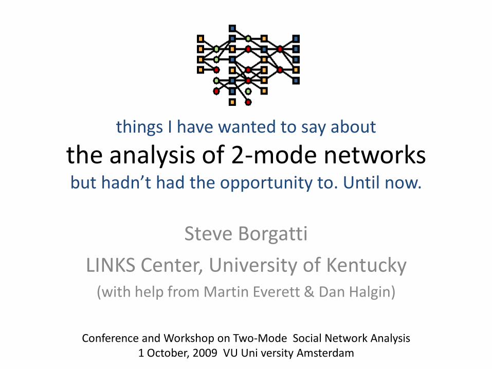
things I have wanted to say about
the analysis of 2-mode networks but hadn’t had the opportunity to. Until now.
Steve Borgatti
LINKS Center, University of Kentucky(with help from Martin Everett & Dan Halgin)
Conference and Workshop on Two-Mode Social Network Analysis1 October, 2009 VU Uni versity Amsterdam
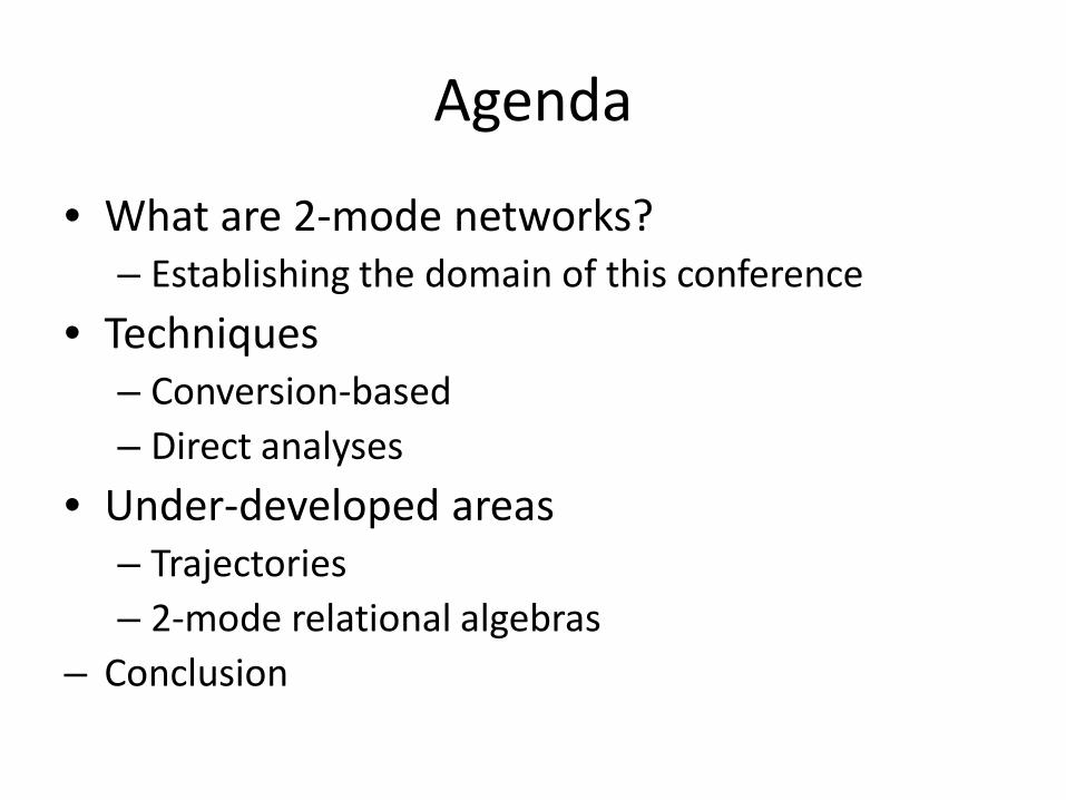
Agenda
• What are 2-mode networks? – Establishing the domain of this conference
• Techniques– Conversion-based– Direct analyses
• Under-developed areas – Trajectories– 2-mode relational algebras
– Conclusion
WHAT ARE 2-MODE NETWORKS?Section 1
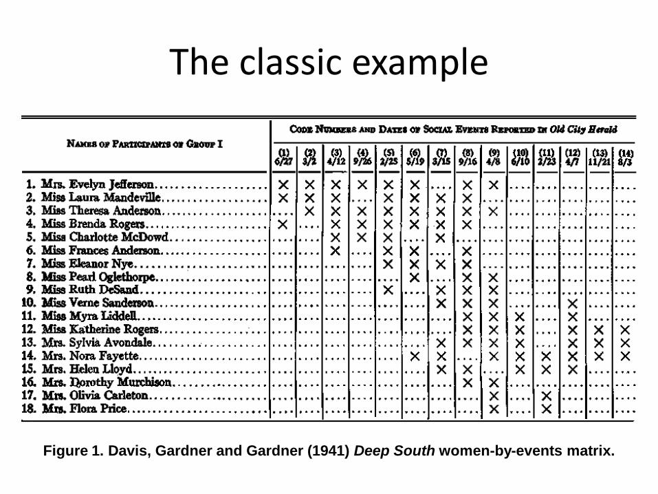
The classic example
Figure 1. Davis, Gardner and Gardner (1941) Deep South women-by-events matrix.
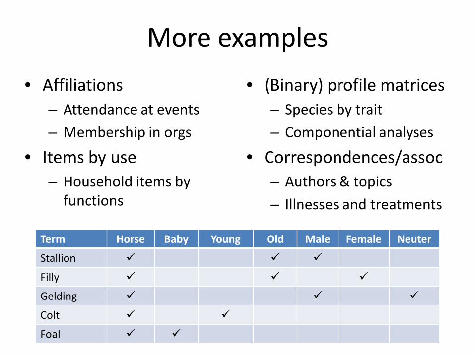
More examples
• Affiliations– Attendance at events
– Membership in orgs
• Items by use– Household items by
functions
• (Binary) profile matrices– Species by trait
– Componential analyses
• Correspondences/assoc– Authors & topics
– Illnesses and treatments
Term Horse Baby Young Old Male Female Neuter
Stallion
Filly
Gelding
Colt
Foal
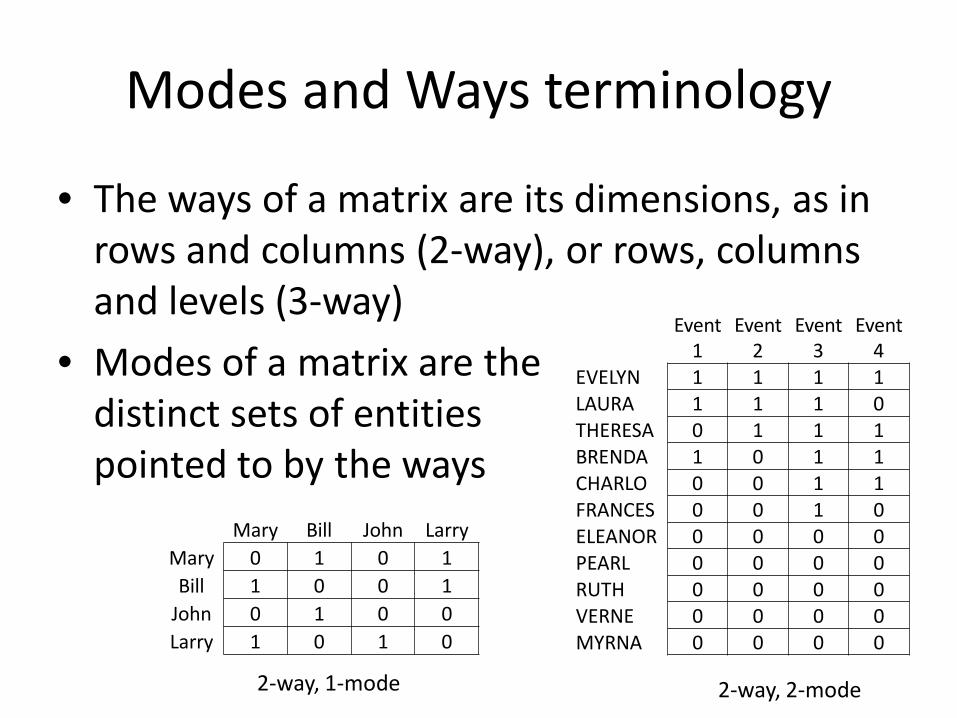
Modes and Ways terminology
• The ways of a matrix are its dimensions, as in rows and columns (2-way), or rows, columns and levels (3-way)
• Modes of a matrix are the distinct sets of entities pointed to by the ways
Event 1
Event 2
Event 3
Event 4
EVELYN 1 1 1 1LAURA 1 1 1 0THERESA 0 1 1 1BRENDA 1 0 1 1CHARLO 0 0 1 1FRANCES 0 0 1 0ELEANOR 0 0 0 0PEARL 0 0 0 0RUTH 0 0 0 0VERNE 0 0 0 0MYRNA 0 0 0 0
Mary Bill John LarryMary 0 1 0 1Bill 1 0 0 1
John 0 1 0 0Larry 1 0 1 0
2-way, 2-mode2-way, 1-mode
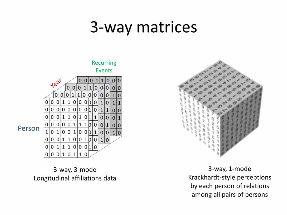
3-way matrices
3-way, 1-modeKrackhardt-style perceptions by each person of relations among all pairs of persons
0 0 0 1 1 0 0 00 0 0 0 0 0 0 00 0 0 1 1 0 1 00 0 0 0 0 1 1 11 0 1 0 0 1 0 00 0 0 1 1 0 0 10 0 1 1 1 0 0 00 0 0 1 0 1 1 0
0 0 0 1 1 0 0 00 0 0 0 0 0 0 00 0 0 1 1 0 1 00 0 0 0 0 1 1 11 0 1 0 0 1 0 00 0 0 1 1 0 0 10 0 1 1 1 0 0 00 0 0 1 0 1 1 0
0 0 0 1 1 0 0 00 0 0 0 0 0 0 00 0 0 1 1 0 1 00 0 0 0 0 1 1 11 0 1 0 0 1 0 00 0 0 1 1 0 0 10 0 1 1 1 0 0 00 0 0 1 0 1 1 0
0 0 0 1 1 0 0 00 0 0 0 0 0 0 00 0 0 1 1 0 1 00 0 0 0 0 1 1 11 0 1 0 0 1 0 00 0 0 1 1 0 0 10 0 1 1 1 0 0 00 0 0 1 0 1 1 0
Person
RecurringEvents
3-way, 3-modeLongitudinal affiliations data
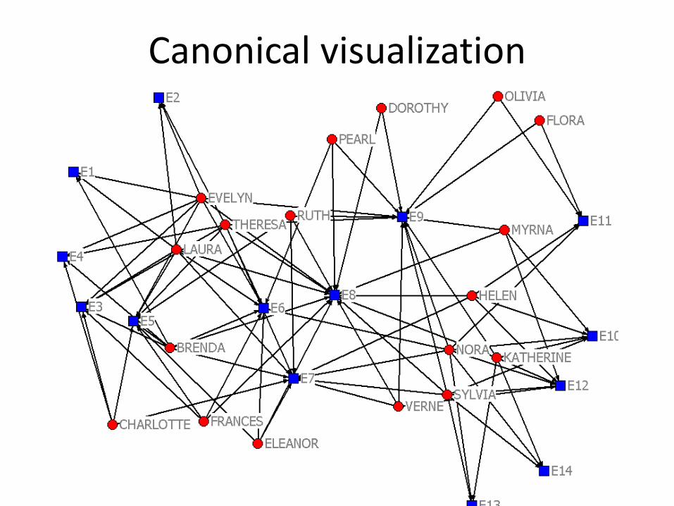
Canonical visualization
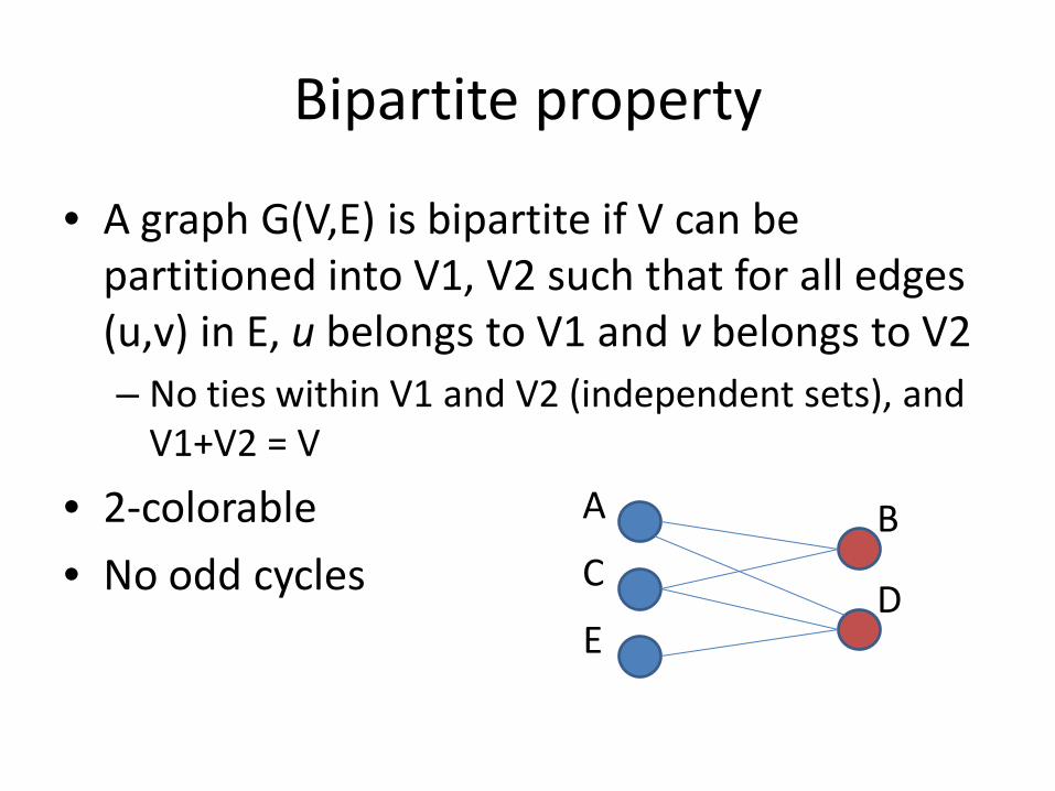
Bipartite property
• A graph G(V,E) is bipartite if V can be partitioned into V1, V2 such that for all edges (u,v) in E, u belongs to V1 and v belongs to V2– No ties within V1 and V2 (independent sets), and
V1+V2 = V
• 2-colorable
• No odd cycles
A
C
ED
B
Two small points
• Bipartite and 2-mode are not interchangeable
• “2-mode network” terminology is misleading

Accidental bipartite-ism
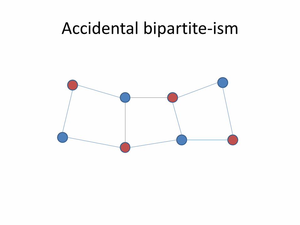
Accidental bipartite-ism
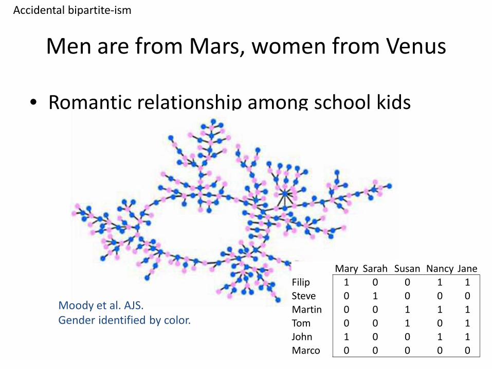
Men are from Mars, women from Venus
• Romantic relationship among school kids
Moody et al. AJS.Gender identified by color.
Mary Sarah Susan Nancy JaneFilip 1 0 0 1 1Steve 0 1 0 0 0Martin 0 0 1 1 1Tom 0 0 1 0 1John 1 0 0 1 1Marco 0 0 0 0 0
Accidental bipartite-ism
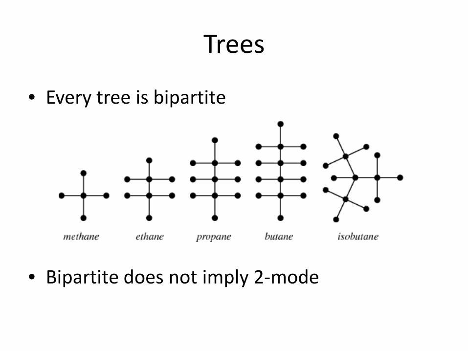
Trees
• Every tree is bipartite
• Bipartite does not imply 2-mode
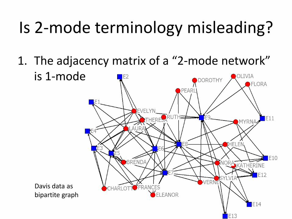
Is 2-mode terminology misleading?
1. The adjacency matrix of a “2-mode network” is 1-mode
Davis data as bipartite graph
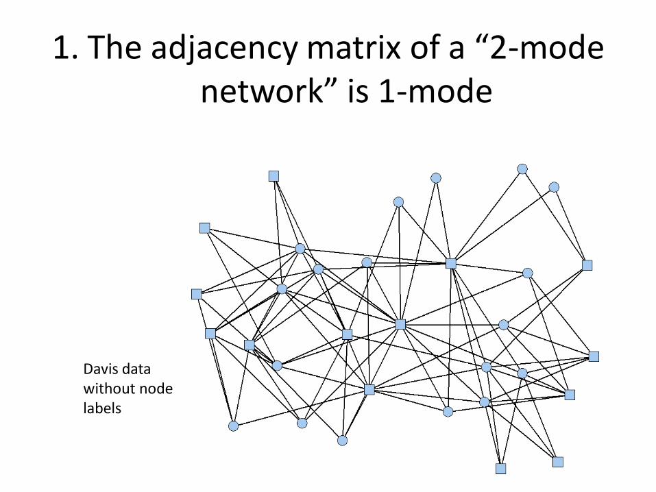
1. The adjacency matrix of a “2-mode network” is 1-mode
Davis data without node labels
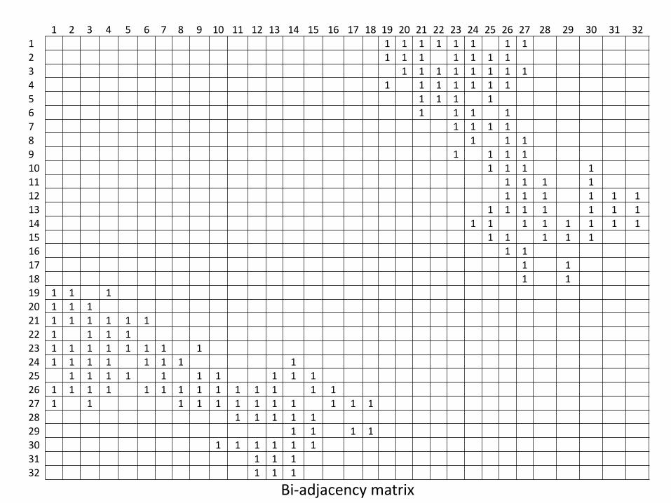
1 2 3 4 5 6 7 8 9 10 11 12 13 14 15 16 17 18 19 20 21 22 23 24 25 26 27 28 29 30 31 321 1 1 1 1 1 1 1 12 1 1 1 1 1 1 13 1 1 1 1 1 1 1 14 1 1 1 1 1 1 15 1 1 1 16 1 1 1 17 1 1 1 18 1 1 19 1 1 1 110 1 1 1 111 1 1 1 112 1 1 1 1 1 113 1 1 1 1 1 1 114 1 1 1 1 1 1 1 115 1 1 1 1 116 1 117 1 118 1 119 1 1 120 1 1 121 1 1 1 1 1 122 1 1 1 123 1 1 1 1 1 1 1 124 1 1 1 1 1 1 1 125 1 1 1 1 1 1 1 1 1 126 1 1 1 1 1 1 1 1 1 1 1 1 1 127 1 1 1 1 1 1 1 1 1 1 1 128 1 1 1 1 129 1 1 1 130 1 1 1 1 1 131 1 1 132 1 1 1
Bi-adjacency matrix
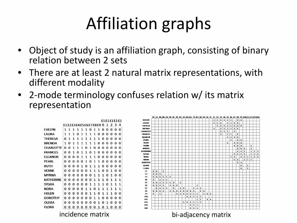
Affiliation graphs• Object of study is an affiliation graph, consisting of binary
relation between 2 sets• There are at least 2 natural matrix representations, with
different modality• 2-mode terminology confuses relation w/ its matrix
representation
incidence matrix bi-adjacency matrix
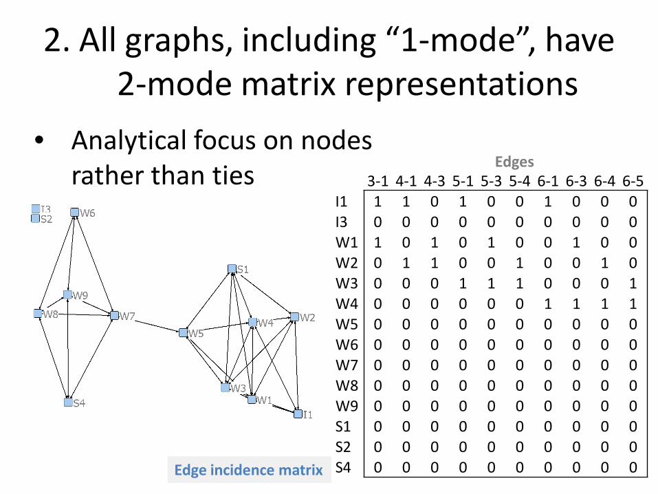
2. All graphs, including “1-mode”, have 2-mode matrix representations
• Analytical focus on nodes rather than ties 3-1 4-1 4-3 5-1 5-3 5-4 6-1 6-3 6-4 6-5
I1 1 1 0 1 0 0 1 0 0 0I3 0 0 0 0 0 0 0 0 0 0W1 1 0 1 0 1 0 0 1 0 0W2 0 1 1 0 0 1 0 0 1 0W3 0 0 0 1 1 1 0 0 0 1W4 0 0 0 0 0 0 1 1 1 1W5 0 0 0 0 0 0 0 0 0 0W6 0 0 0 0 0 0 0 0 0 0W7 0 0 0 0 0 0 0 0 0 0W8 0 0 0 0 0 0 0 0 0 0W9 0 0 0 0 0 0 0 0 0 0S1 0 0 0 0 0 0 0 0 0 0S2 0 0 0 0 0 0 0 0 0 0S4 0 0 0 0 0 0 0 0 0 0Edge incidence matrix
Edges
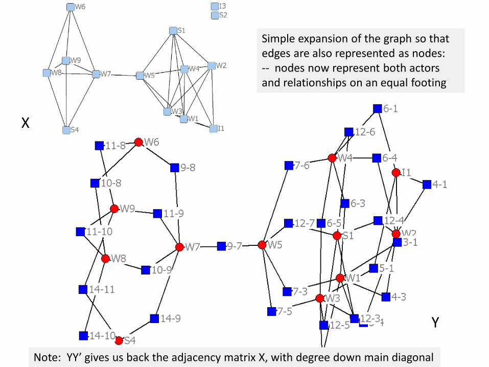
Simple expansion of the graph so that edges are also represented as nodes:-- nodes now represent both actors and relationships on an equal footing
Note: YY’ gives us back the adjacency matrix X, with degree down main diagonal
X
Y
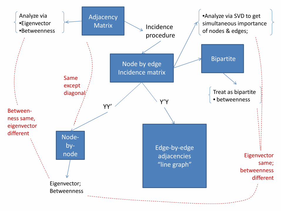
Adjacency Matrix Incidence
procedure
Node by edgeIncidence matrix
Node-by-
node
YY’Y’Y
Edge-by-edge adjacencies“line graph”
Same exceptdiagonal
Eigenvector;Betweenness
Treat as bipartite• betweenness
Analyze via•Eigenvector•Betweenness
Eigenvector same;
betweenness different
Between-ness same, eigenvector different
•Analyze via SVD to get simultaneous importance of nodes & edges;
Bipartite
R1
R2
R3
R4
R5 R6
C1
C2
C3
C4
C5
C6
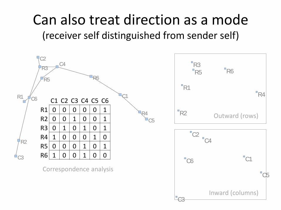
Can also treat direction as a mode(receiver self distinguished from sender self)
C1 C2 C3 C4 C5 C6R1 0 0 0 0 0 1R2 0 0 1 0 0 1R3 0 1 0 1 0 1R4 1 0 0 0 1 0R5 0 0 0 1 0 1R6 1 0 0 1 0 0
R1
R2
R3
R4
R5 R6
C1
C2
C3
C4
C5
C6
Outward (rows)
Inward (columns)
Correspondence analysis
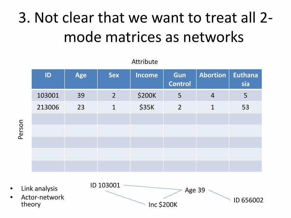
3. Not clear that we want to treat all 2-mode matrices as networks
ID Age Sex Income Gun Control
Abortion Euthanasia
103001 39 2 $200K 5 4 5
213006 23 1 $35K 2 1 53
Pers
on
Attribute
ID 103001Age 39
Inc $200KID 656002
• Link analysis• Actor-network
theory
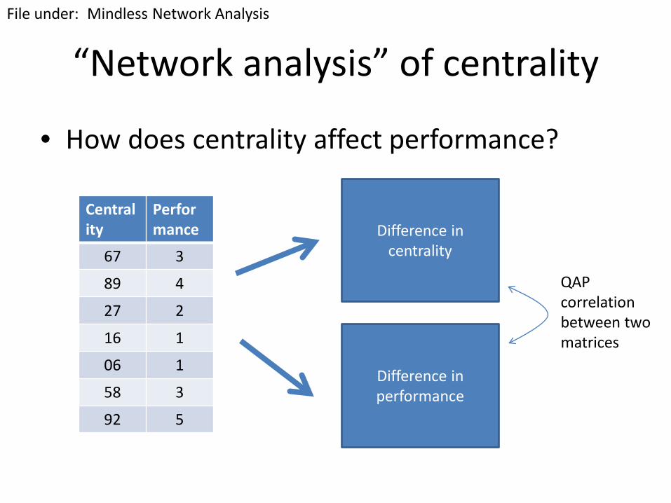
“Network analysis” of centrality
• How does centrality affect performance?
Centrality
Performance
67 3
89 4
27 2
16 1
06 1
58 3
92 5
Difference in centrality
Difference in performance
QAP correlation between two matrices
File under: Mindless Network Analysis
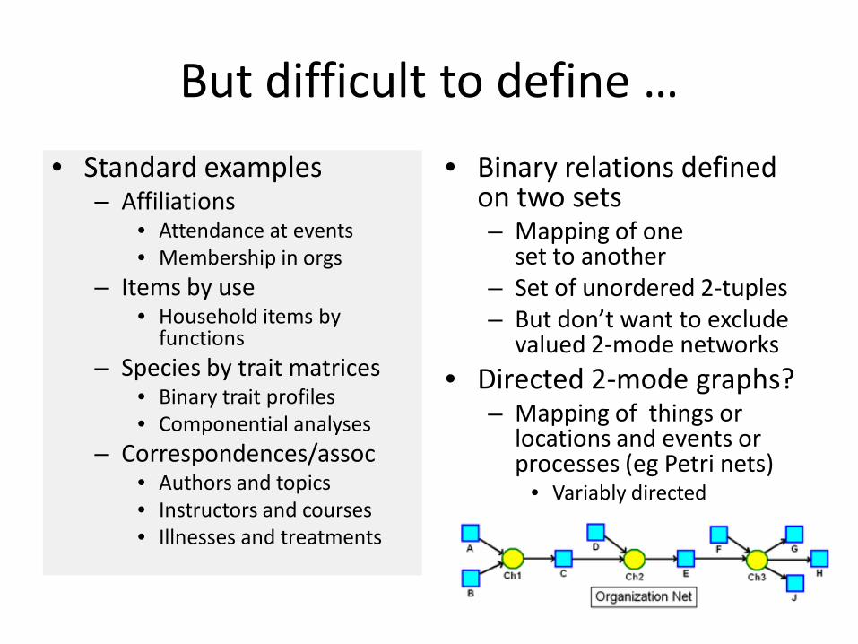
But difficult to define …
• Standard examples– Affiliations
• Attendance at events• Membership in orgs
– Items by use• Household items by
functions– Species by trait matrices
• Binary trait profiles• Componential analyses
– Correspondences/assoc• Authors and topics• Instructors and courses• Illnesses and treatments
• Binary relations defined on two sets– Mapping of one
set to another– Set of unordered 2-tuples– But don’t want to exclude
valued 2-mode networks• Directed 2-mode graphs?
– Mapping of things or locations and events or processes (eg Petri nets)
• Variably directed
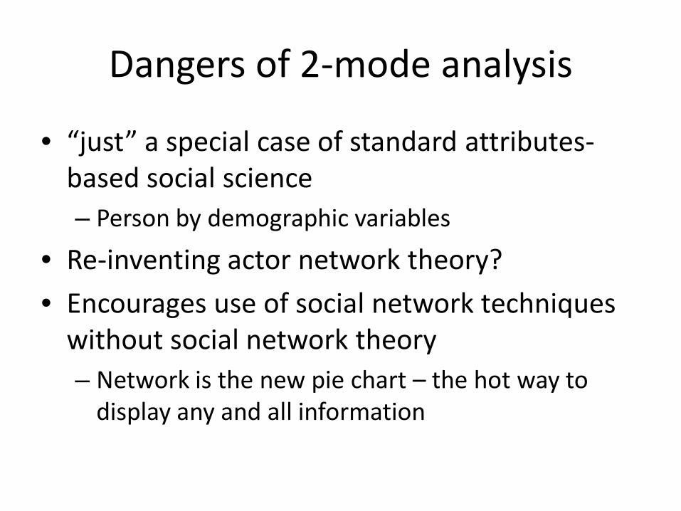
Dangers of 2-mode analysis
• “just” a special case of standard attributes-based social science– Person by demographic variables
• Re-inventing actor network theory?
• Encourages use of social network techniques without social network theory– Network is the new pie chart – the hot way to
display any and all information

TECHNIQUESSection 2
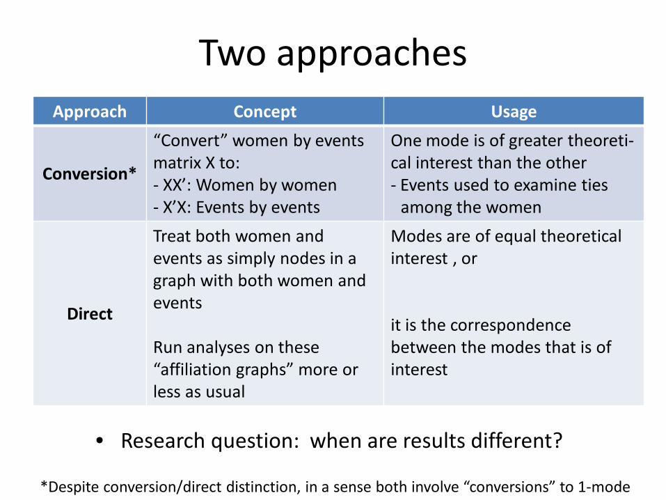
Two approachesApproach Concept Usage
Conversion*
“Convert” women by events matrix X to:- XX’: Women by women- X’X: Events by events
One mode is of greater theoreti-cal interest than the other- Events used to examine ties
among the women
Direct
Treat both women and events as simply nodes in a graph with both women and events
Run analyses on these “affiliation graphs” more or less as usual
Modes are of equal theoretical interest , or
it is the correspondence between the modes that is of interest
*Despite conversion/direct distinction, in a sense both involve “conversions” to 1-mode
• Research question: when are results different?

CONVERSION APPROACHSection 2A
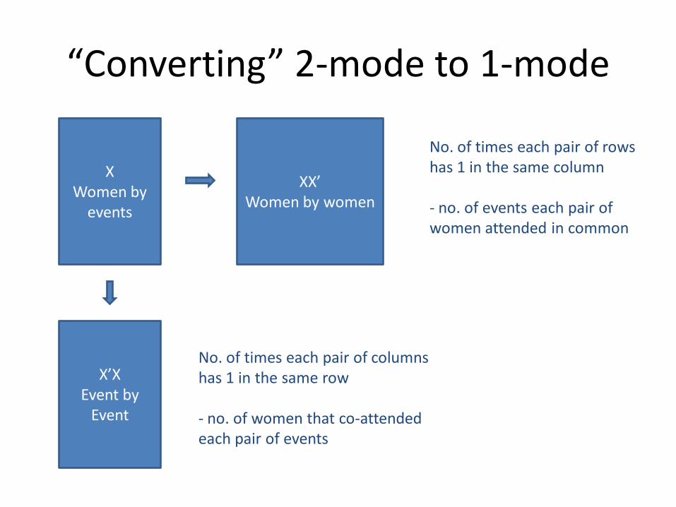
“Converting” 2-mode to 1-mode
XWomen by
events
XX’Women by women
X’XEvent by
Event
No. of times each pair of rows has 1 in the same column
- no. of events each pair of women attended in common
No. of times each pair of columns has 1 in the same row
- no. of women that co-attended each pair of events
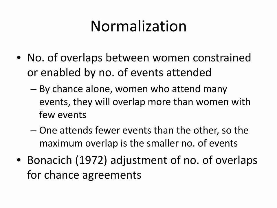
Normalization
• No. of overlaps between women constrained or enabled by no. of events attended– By chance alone, women who attend many
events, they will overlap more than women with few events
– One attends fewer events than the other, so the maximum overlap is the smaller no. of events
• Bonacich (1972) adjustment of no. of overlaps for chance agreements
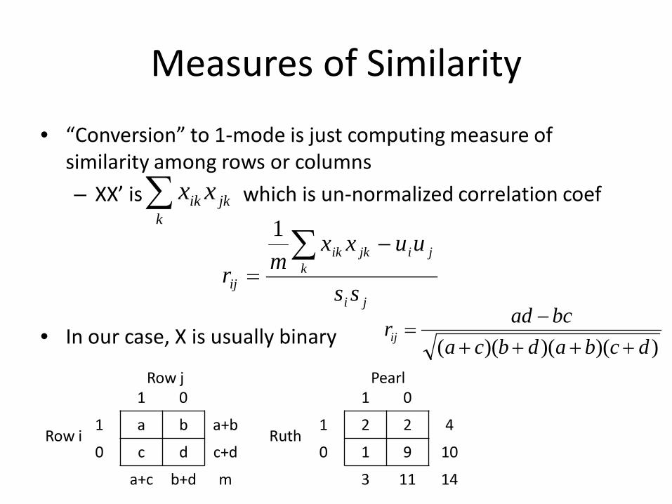
Measures of Similarity
• “Conversion” to 1-mode is just computing measure of similarity among rows or columns
– XX’ is which is un-normalized correlation coefjkk
ik xx∑
ji
jijkk
ik
ij ss
uuxxmr
−=
∑1
• In our case, X is usually binary
1 0
1 2 2 4
0 1 9 10
3 11 14
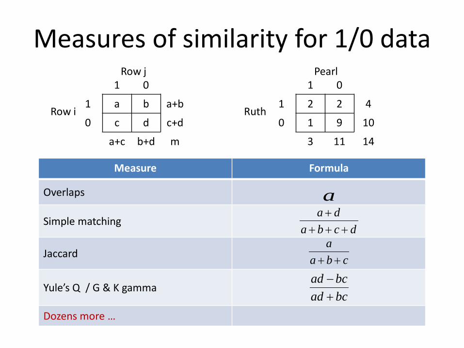
1 0
1 a b a+b
0 c d c+d
a+c b+d m
Row i
Row j
Ruth
Pearl
))()()(( dcbadbcabcadrij ++++
−=
Measure Formula
Overlaps
Simple matching
Jaccard
Yule’s Q / G & K gamma
Dozens more …
bcadbcad
+−
1 0
1 2 2 4
0 1 9 10
3 11 14
Measures of similarity for 1/0 data
1 0
1 a b a+b
0 c d c+d
a+c b+d m
Row i
Row j
Ruth
Pearl
a
dcbada+++
+
cbaa++
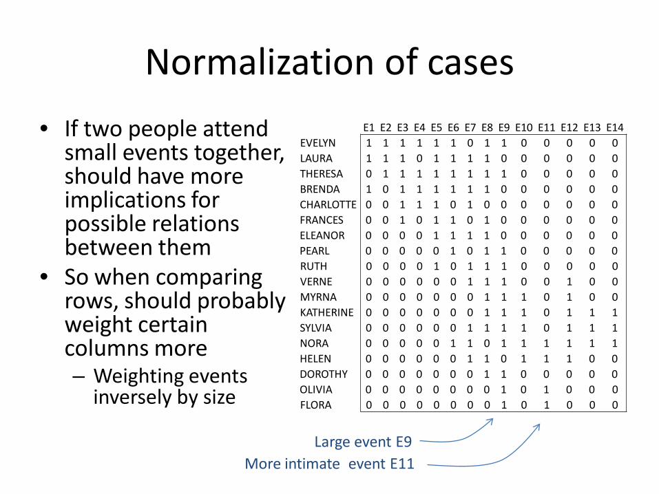
Normalization of cases
• If two people attend small events together, should have more implications for possible relations between them
• So when comparing rows, should probably weight certain columns more– Weighting events
inversely by size
E1 E2 E3 E4 E5 E6 E7 E8 E9 E10 E11 E12 E13 E14EVELYN 1 1 1 1 1 1 0 1 1 0 0 0 0 0LAURA 1 1 1 0 1 1 1 1 0 0 0 0 0 0THERESA 0 1 1 1 1 1 1 1 1 0 0 0 0 0BRENDA 1 0 1 1 1 1 1 1 0 0 0 0 0 0CHARLOTTE 0 0 1 1 1 0 1 0 0 0 0 0 0 0FRANCES 0 0 1 0 1 1 0 1 0 0 0 0 0 0ELEANOR 0 0 0 0 1 1 1 1 0 0 0 0 0 0PEARL 0 0 0 0 0 1 0 1 1 0 0 0 0 0RUTH 0 0 0 0 1 0 1 1 1 0 0 0 0 0VERNE 0 0 0 0 0 0 1 1 1 0 0 1 0 0MYRNA 0 0 0 0 0 0 0 1 1 1 0 1 0 0KATHERINE 0 0 0 0 0 0 0 1 1 1 0 1 1 1SYLVIA 0 0 0 0 0 0 1 1 1 1 0 1 1 1NORA 0 0 0 0 0 1 1 0 1 1 1 1 1 1HELEN 0 0 0 0 0 0 1 1 0 1 1 1 0 0DOROTHY 0 0 0 0 0 0 0 1 1 0 0 0 0 0OLIVIA 0 0 0 0 0 0 0 0 1 0 1 0 0 0FLORA 0 0 0 0 0 0 0 0 1 0 1 0 0 0
Large event E9More intimate event E11
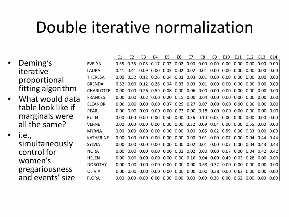
Double iterative normalization
• Deming’s iterative proportional fitting algorithm
• What would data table look like if marginals were all the same?
• i.e., simultaneously control for women’s gregariousness and events’ size
E1 E2 E3 E4 E5 E6 E7 E8 E9 E10 E11 E12 E13 E14EVELYN 0.35 0.35 0.08 0.17 0.02 0.02 0.00 0.00 0.00 0.00 0.00 0.00 0.00 0.00LAURA 0.41 0.41 0.09 0.00 0.03 0.02 0.02 0.01 0.00 0.00 0.00 0.00 0.00 0.00THERESA 0.00 0.52 0.12 0.26 0.04 0.03 0.03 0.01 0.00 0.00 0.00 0.00 0.00 0.00BRENDA 0.52 0.00 0.12 0.26 0.04 0.03 0.03 0.01 0.00 0.00 0.00 0.00 0.00 0.00CHARLOTTE 0.00 0.00 0.26 0.59 0.08 0.00 0.06 0.00 0.00 0.00 0.00 0.00 0.00 0.00FRANCES 0.00 0.00 0.62 0.00 0.20 0.15 0.00 0.04 0.00 0.00 0.00 0.00 0.00 0.00ELEANOR 0.00 0.00 0.00 0.00 0.37 0.29 0.27 0.07 0.00 0.00 0.00 0.00 0.00 0.00PEARL 0.00 0.00 0.00 0.00 0.00 0.73 0.00 0.18 0.09 0.00 0.00 0.00 0.00 0.00RUTH 0.00 0.00 0.00 0.00 0.50 0.00 0.36 0.10 0.05 0.00 0.00 0.00 0.00 0.00VERNE 0.00 0.00 0.00 0.00 0.00 0.00 0.32 0.09 0.04 0.00 0.00 0.55 0.00 0.00MYRNA 0.00 0.00 0.00 0.00 0.00 0.00 0.00 0.05 0.02 0.59 0.00 0.33 0.00 0.00KATHERINE 0.00 0.00 0.00 0.00 0.00 0.00 0.00 0.01 0.00 0.07 0.00 0.04 0.44 0.44SYLVIA 0.00 0.00 0.00 0.00 0.00 0.00 0.02 0.01 0.00 0.07 0.00 0.04 0.43 0.43NORA 0.00 0.00 0.00 0.00 0.00 0.02 0.02 0.00 0.00 0.07 0.00 0.04 0.42 0.42HELEN 0.00 0.00 0.00 0.00 0.00 0.00 0.16 0.04 0.00 0.49 0.03 0.28 0.00 0.00DOROTHY 0.00 0.00 0.00 0.00 0.00 0.00 0.00 0.68 0.32 0.00 0.00 0.00 0.00 0.00OLIVIA 0.00 0.00 0.00 0.00 0.00 0.00 0.00 0.00 0.38 0.00 0.62 0.00 0.00 0.00FLORA 0.00 0.00 0.00 0.00 0.00 0.00 0.00 0.00 0.38 0.00 0.62 0.00 0.00 0.00
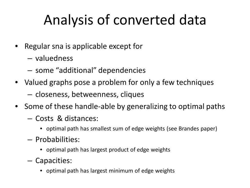
Analysis of converted data
• Regular sna is applicable except for
– valuedness
– some “additional” dependencies
• Valued graphs pose a problem for only a few techniques
– closeness, betweenness, cliques
• Some of these handle-able by generalizing to optimal paths
– Costs & distances: • optimal path has smallest sum of edge weights (see Brandes paper)
– Probabilities: • optimal path has largest product of edge weights
– Capacities: • optimal path has largest minimum of edge weights
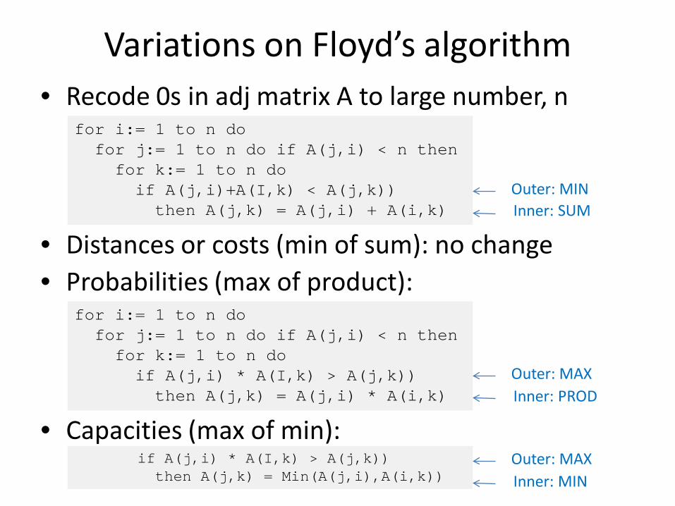
Variations on Floyd’s algorithm• Recode 0s in adj matrix A to large number, n
• Distances or costs (min of sum): no change• Probabilities (max of product):
• Capacities (max of min):
for i:= 1 to n dofor j:= 1 to n do if A(j,i) < n thenfor k:= 1 to n do
if A(j,i)+A(I,k) < A(j,k))then A(j,k) = A(j,i) + A(i,k)
for i:= 1 to n dofor j:= 1 to n do if A(j,i) < n thenfor k:= 1 to n do
if A(j,i) * A(I,k) > A(j,k))then A(j,k) = A(j,i) * A(i,k)
if A(j,i) * A(I,k) > A(j,k))then A(j,k) = Min(A(j,i),A(i,k))
Outer: MINInner: SUM
Outer: MAXInner: PROD
Outer: MAXInner: MIN
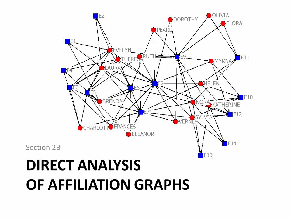
DIRECT ANALYSISOF AFFILIATION GRAPHS
Section 2B
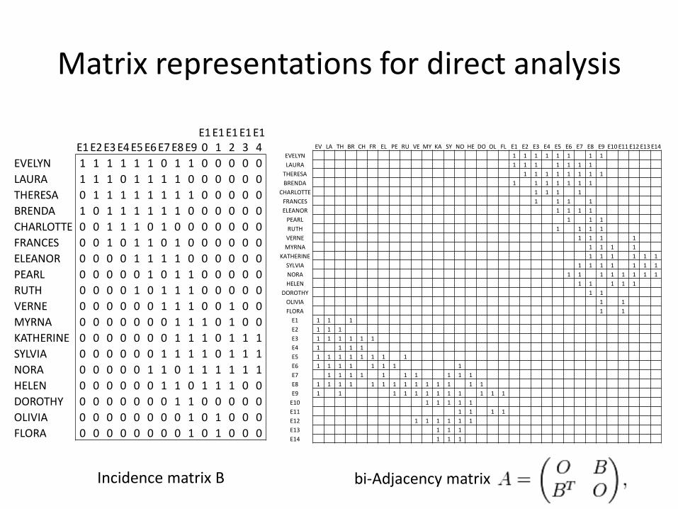
Matrix representations for direct analysis
EV LA TH BR CH FR EL PE RU VE MY KA SY NO HE DO OL FL E1 E2 E3 E4 E5 E6 E7 E8 E9 E10 E11 E12 E13 E14EVELYN 1 1 1 1 1 1 1 1LAURA 1 1 1 1 1 1 1
THERESA 1 1 1 1 1 1 1 1BRENDA 1 1 1 1 1 1 1
CHARLOTTE 1 1 1 1FRANCES 1 1 1 1ELEANOR 1 1 1 1
PEARL 1 1 1RUTH 1 1 1 1VERNE 1 1 1 1MYRNA 1 1 1 1
KATHERINE 1 1 1 1 1 1SYLVIA 1 1 1 1 1 1 1NORA 1 1 1 1 1 1 1 1HELEN 1 1 1 1 1
DOROTHY 1 1OLIVIA 1 1FLORA 1 1
E1 1 1 1E2 1 1 1E3 1 1 1 1 1 1E4 1 1 1 1E5 1 1 1 1 1 1 1 1E6 1 1 1 1 1 1 1 1E7 1 1 1 1 1 1 1 1 1 1E8 1 1 1 1 1 1 1 1 1 1 1 1 1 1E9 1 1 1 1 1 1 1 1 1 1 1 1
E10 1 1 1 1 1E11 1 1 1 1E12 1 1 1 1 1 1E13 1 1 1E14 1 1 1
E1 E2 E3 E4 E5 E6 E7 E8 E9E10
E11
E12
E13
E14
EVELYN 1 1 1 1 1 1 0 1 1 0 0 0 0 0LAURA 1 1 1 0 1 1 1 1 0 0 0 0 0 0THERESA 0 1 1 1 1 1 1 1 1 0 0 0 0 0BRENDA 1 0 1 1 1 1 1 1 0 0 0 0 0 0CHARLOTTE 0 0 1 1 1 0 1 0 0 0 0 0 0 0FRANCES 0 0 1 0 1 1 0 1 0 0 0 0 0 0ELEANOR 0 0 0 0 1 1 1 1 0 0 0 0 0 0PEARL 0 0 0 0 0 1 0 1 1 0 0 0 0 0RUTH 0 0 0 0 1 0 1 1 1 0 0 0 0 0VERNE 0 0 0 0 0 0 1 1 1 0 0 1 0 0MYRNA 0 0 0 0 0 0 0 1 1 1 0 1 0 0KATHERINE 0 0 0 0 0 0 0 1 1 1 0 1 1 1SYLVIA 0 0 0 0 0 0 1 1 1 1 0 1 1 1NORA 0 0 0 0 0 1 1 0 1 1 1 1 1 1HELEN 0 0 0 0 0 0 1 1 0 1 1 1 0 0DOROTHY 0 0 0 0 0 0 0 1 1 0 0 0 0 0OLIVIA 0 0 0 0 0 0 0 0 1 0 1 0 0 0FLORA 0 0 0 0 0 0 0 0 1 0 1 0 0 0
Incidence matrix B bi-Adjacency matrix
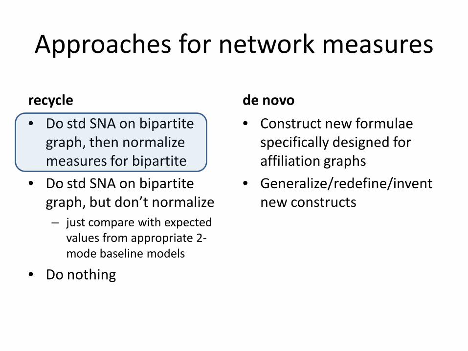
Approaches for network measures
recycle
• Do std SNA on bipartite graph, then normalize measures for bipartite
• Do std SNA on bipartite graph, but don’t normalize– just compare with expected
values from appropriate 2-mode baseline models
• Do nothing
de novo
• Construct new formulae specifically designed for affiliation graphs
• Generalize/redefine/invent new constructs
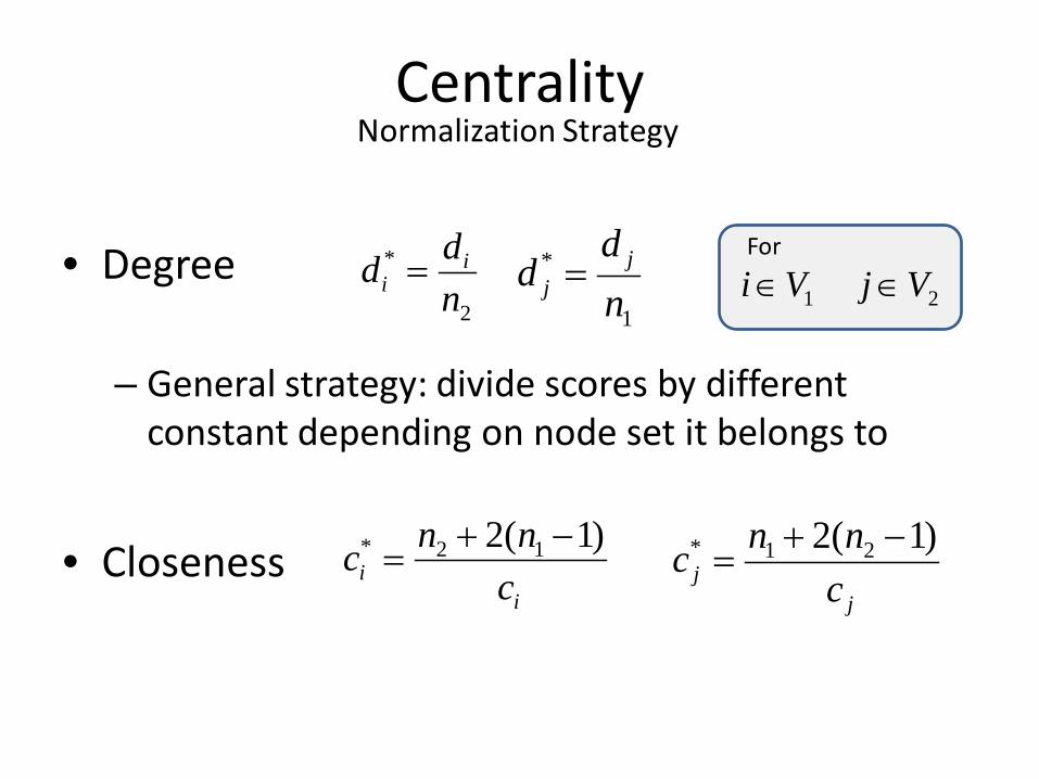
Centrality
• Degree
– General strategy: divide scores by different constant depending on node set it belongs to
• Closeness
Normalization Strategy
2
*
ndd i
i =1
*
nd
d jj =
ii c
nnc )1(2 12* −+=
jj c
nnc )1(2 21* −+=
1Vi∈ 2Vj∈For
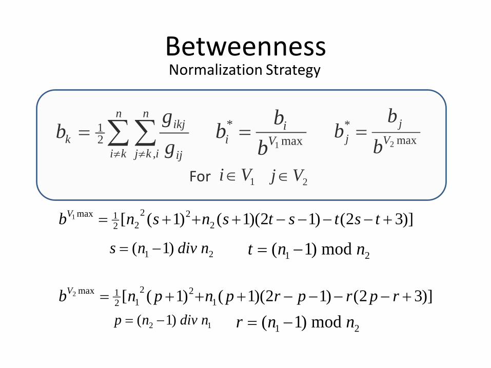
Betweenness
∑∑≠ ≠
=n
ki
n
ikj ij
ikjk g
gb
,21
)]32()12)(1()1([ 222
221max1 +−−−−+++= tststsnsnbV
21 )1( ndivns −=
max*
1Vi
i bbb = max
*2V
jj b
bb =
1Vi∈ 2Vj∈
21 mod)1( nnt −=
)]32()12)(1()1([ 122
121max2 +−−−−+++= rprprpnpnbV
12 )1( ndivnp −=21 mod)1( nnr −=
Normalization Strategy
For
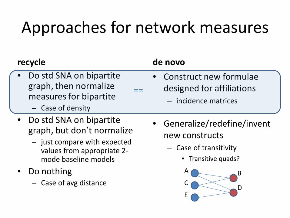
Approaches for network measures
recycle• Do std SNA on bipartite
graph, then normalize measures for bipartite – Case of density
• Do std SNA on bipartite graph, but don’t normalize– just compare with expected
values from appropriate 2-mode baseline models
• Do nothing– Case of avg distance
de novo
• Construct new formulae designed for affiliations– incidence matrices
• Generalize/redefine/invent new constructs– Case of transitivity
• Transitive quads?
A
C
ED
B
==
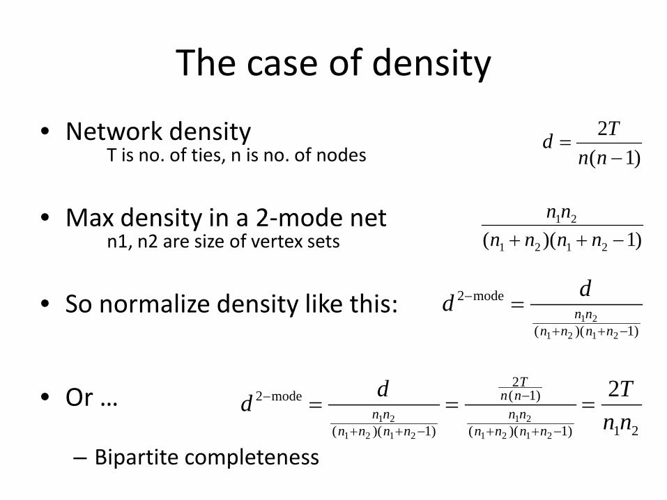
The case of density
• Network densityT is no. of ties, n is no. of nodes
• Max density in a 2-mode netn1, n2 are size of vertex sets
• So normalize density like this:
• Or …
– Bipartite completeness
)1(2−
=nn
Td
)1)(( 2121
21
−++ nnnnnn
)1)((
mode2
2121
21−++
− =nnnn
nndd
21)1)((
)1(2
)1)((
mode2 2
2121
21
2121
21 nnTdd
nnnnnn
nnT
nnnnnn ===
−++
−
−++
−
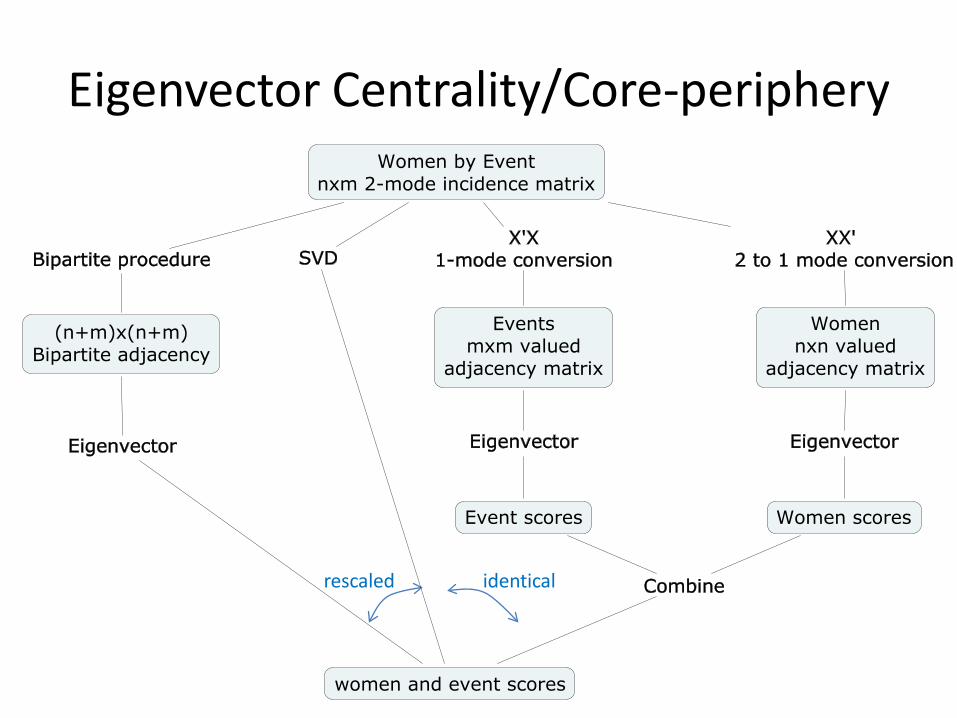
Eigenvector Centrality/Core-periphery
rescaled identical
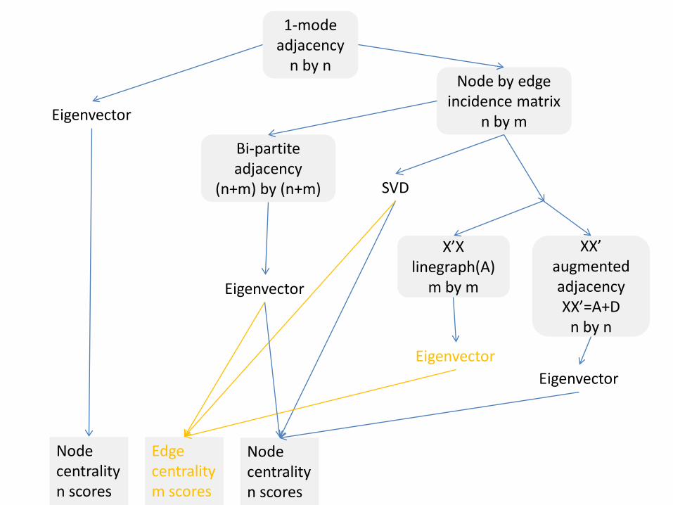
1-mode adjacency
n by n
Eigenvector
Nodecentralityn scores
Node by edge incidence matrix
n by m
SVD
XX’augmented adjacencyXX’=A+D
n by n
X’Xlinegraph(A)
m by m
EigenvectorEigenvector
Edgecentralitym scores
Bi-partite adjacency
(n+m) by (n+m)
Eigenvector
Nodecentralityn scores
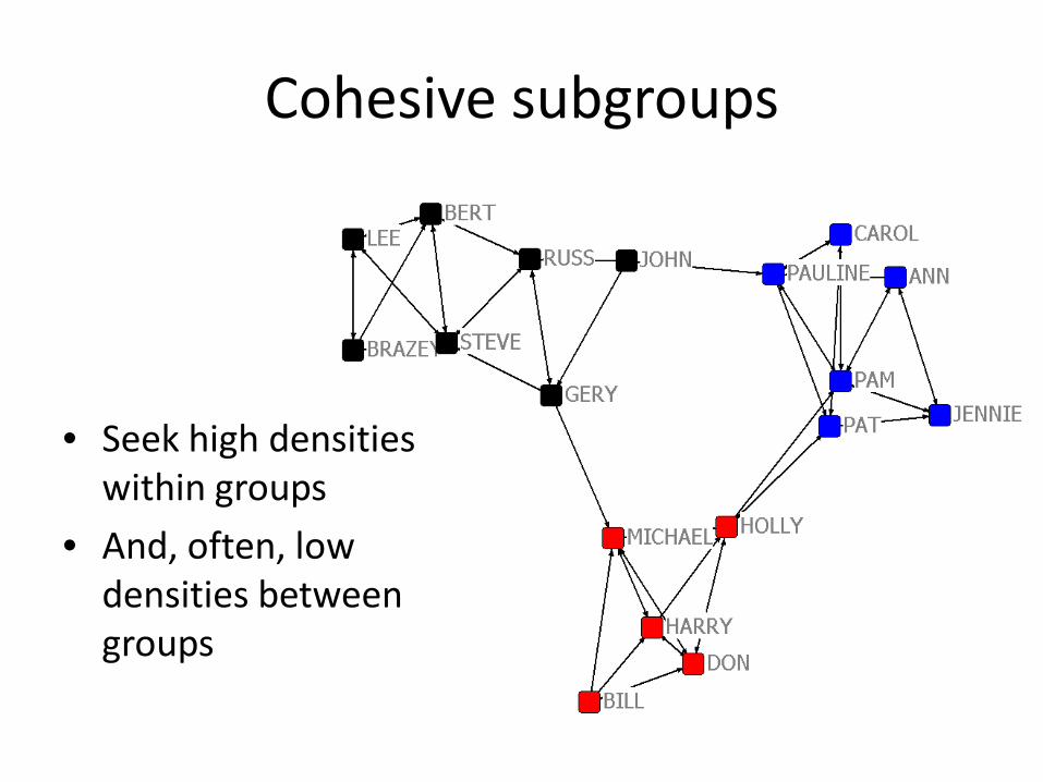
Cohesive subgroups
• Seek high densities within groups
• And, often, low densities between groups
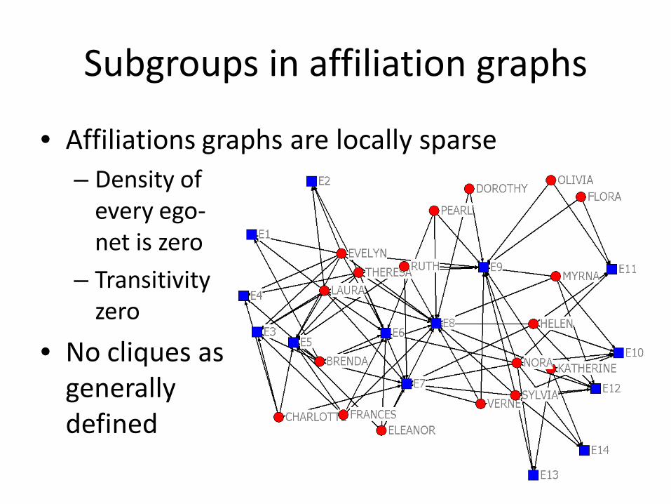
Subgroups in affiliation graphs
• Affiliations graphs are locally sparse– Density of
every ego-net is zero
– Transitivityzero
• No cliques as generally defined
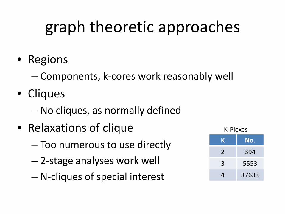
graph theoretic approaches
• Regions – Components, k-cores work reasonably well
• Cliques– No cliques, as normally defined
• Relaxations of clique– Too numerous to use directly
– 2-stage analyses work well
– N-cliques of special interest
K No.
2 394
3 5553
4 37633
K-Plexes
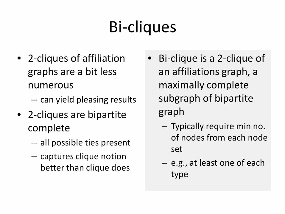
Bi-cliques
• 2-cliques of affiliation graphs are a bit less numerous– can yield pleasing results
• 2-cliques are bipartite complete– all possible ties present
– captures clique notion better than clique does
• Bi-clique is a 2-clique of an affiliations graph, a maximally complete subgraph of bipartite graph– Typically require min no.
of nodes from each node set
– e.g., at least one of each type
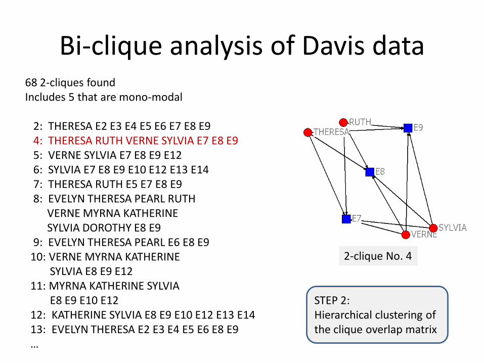
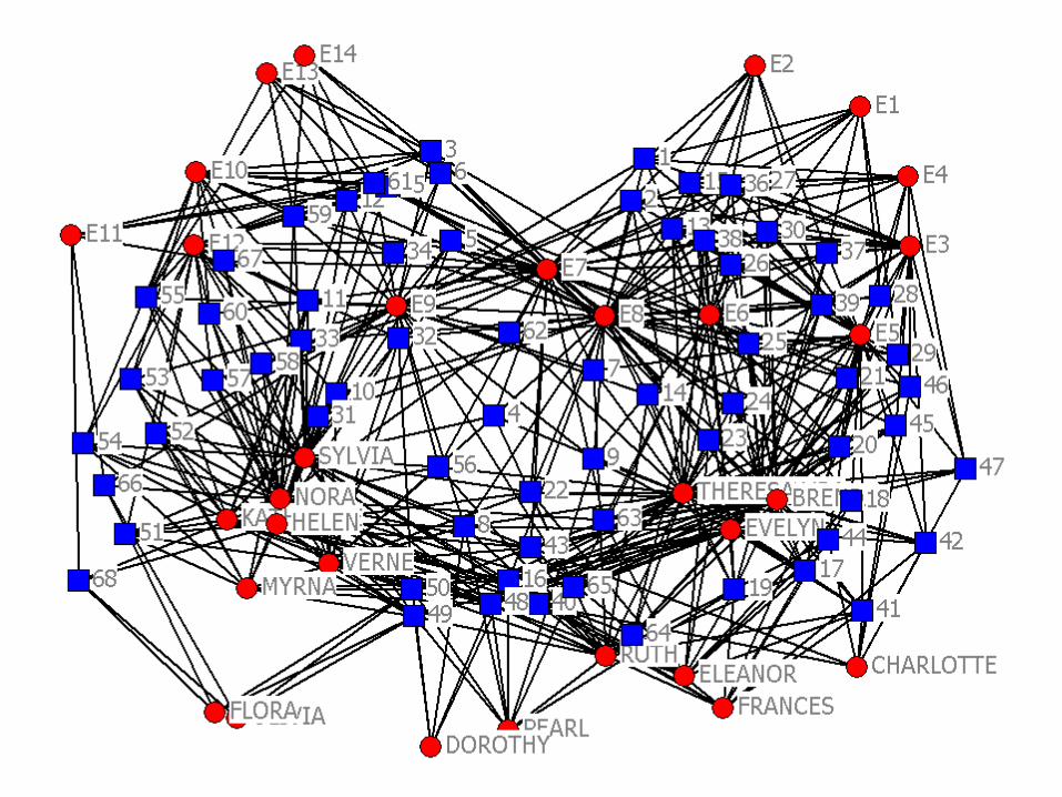
Bi-clique analysis of Davis data68 2-cliques foundIncludes 5 that are mono-modal
2: THERESA E2 E3 E4 E5 E6 E7 E8 E94: THERESA RUTH VERNE SYLVIA E7 E8 E95: VERNE SYLVIA E7 E8 E9 E126: SYLVIA E7 E8 E9 E10 E12 E13 E147: THERESA RUTH E5 E7 E8 E98: EVELYN THERESA PEARL RUTH
VERNE MYRNA KATHERINE SYLVIA DOROTHY E8 E9
9: EVELYN THERESA PEARL E6 E8 E910: VERNE MYRNA KATHERINE
SYLVIA E8 E9 E1211: MYRNA KATHERINE SYLVIA
E8 E9 E10 E1212: KATHERINE SYLVIA E8 E9 E10 E12 E13 E1413: EVELYN THERESA E2 E3 E4 E5 E6 E8 E9…
2-clique No. 4
STEP 2:Hierarchical clustering of the clique overlap matrix
C K H A
D A F E T TO O R R L E H B H S
P R L F L A E V L E R H M E V Y E O I L O N A R E A R E E Y R N E L A T V O T C N U L U E N E L R I E O R V E E ER H I R T E E E O T E Y R S D E E E E E 1 E N N 1 R E N I 1 1 1L Y A A E 2 1 S R H 4 N A A A 7 3 6 5 8 1 N A E 0 A 9 E A 2 3 4
------ - - - - - - - - - - - - - - - - - - - - - - - - - - - - - - - -22.000 . . . . . . . . . . . . . XXX . . . XXX . . . . . . . . . . . .20.000 . . . . . . . . . . . . XXXXX . . XXXXX . . . . . . . . . . . .18.000 . . . . . . . . . . . . XXXXX . . XXXXX . . . . . . . XXX . . .17.000 . . . . . . . . . . . . XXXXX . XXXXXXX . . . . . . . XXX . . .15.250 . . . . . . . . . . . XXXXXXX . XXXXXXX . . . . . . . XXX . . .15.000 . . . . . . . . . . . XXXXXXX XXXXXXXXX . . . . . . . XXX . . .14.667 . . . . . . . . . . . XXXXXXX XXXXXXXXX . . . . . . . XXXXX . .14.033 . . . . . . . . . . . XXXXXXXXXXXXXXXXX . . . . . . . XXXXX . .13.000 . . . . . . . . . . . XXXXXXXXXXXXXXXXX . . XXX . . . XXXXX . .12.000 . . . . . . . . . . . XXXXXXXXXXXXXXXXX . . XXX . . XXXXXXX . .11.747 . . . . . . . . . . . XXXXXXXXXXXXXXXXX . . XXX . XXXXXXXXX . .9.878 . . . . . . . . . . . XXXXXXXXXXXXXXXXX . . XXX XXXXXXXXXXX . .9.000 . . . . . . . . XXX . XXXXXXXXXXXXXXXXX . . XXX XXXXXXXXXXX . .8.975 . . . . . . . . XXX . XXXXXXXXXXXXXXXXX . . XXXXXXXXXXXXXXX . .8.288 . . . . . . . . XXX . XXXXXXXXXXXXXXXXX . XXXXXXXXXXXXXXXXX . .7.069 . . . . . . . . XXX XXXXXXXXXXXXXXXXXXX . XXXXXXXXXXXXXXXXX . .6.245 . . . . . . . . XXXXXXXXXXXXXXXXXXXXXXX . XXXXXXXXXXXXXXXXX . .6.000 . . . . . . . . XXXXXXXXXXXXXXXXXXXXXXX . XXXXXXXXXXXXXXXXX XXX5.143 . . . . . . . XXXXXXXXXXXXXXXXXXXXXXXXX . XXXXXXXXXXXXXXXXX XXX5.000 XXX . . . . . XXXXXXXXXXXXXXXXXXXXXXXXX . XXXXXXXXXXXXXXXXX XXX4.675 XXX . . . . XXXXXXXXXXXXXXXXXXXXXXXXXXX . XXXXXXXXXXXXXXXXX XXX4.464 XXX . . . XXXXXXXXXXXXXXXXXXXXXXXXXXXXX . XXXXXXXXXXXXXXXXX XXX4.000 XXX XXX . XXXXXXXXXXXXXXXXXXXXXXXXXXXXX . XXXXXXXXXXXXXXXXX XXX3.703 XXX XXX . XXXXXXXXXXXXXXXXXXXXXXXXXXXXX . XXXXXXXXXXXXXXXXXXXXX3.126 XXX XXX XXXXXXXXXXXXXXXXXXXXXXXXXXXXXXX . XXXXXXXXXXXXXXXXXXXXX2.188 XXX XXX XXXXXXXXXXXXXXXXXXXXXXXXXXXXXXX XXXXXXXXXXXXXXXXXXXXXXX2.000 XXXXXXX XXXXXXXXXXXXXXXXXXXXXXXXXXXXXXX XXXXXXXXXXXXXXXXXXXXXXX1.788 XXXXXXX XXXXXXXXXXXXXXXXXXXXXXXXXXXXXXXXXXXXXXXXXXXXXXXXXXXXXXX0.860 XXXXXXXXXXXXXXXXXXXXXXXXXXXXXXXXXXXXXXXXXXXXXXXXXXXXXXXXXXXXXXX
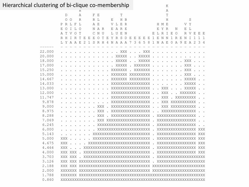
Hierarchical clustering of bi-clique co-membership
C K H A
D A F E T TO O R R L E H B H S
P R L F L A E V L E R H M E V Y E O I L O N A R E A R E E Y R N E L A T V O T C N U L U E N E L R I E O R V E E ER H I R T E E E O T E Y R S D E E E E E 1 E N N 1 R E N I 1 1 1L Y A A E 2 1 S R H 4 N A A A 7 3 6 5 8 1 N A E 0 A 9 E A 2 3 4
------ - - - - - - - - - - - - - - - - - - - - - - - - - - - - - - - -22.000 . . . . . . . . . . . . . XXX . . . XXX . . . . . . . . . . . .20.000 . . . . . . . . . . . . XXXXX . . XXXXX . . . . . . . . . . . .18.000 . . . . . . . . . . . . XXXXX . . XXXXX . . . . . . . XXX . . .17.000 . . . . . . . . . . . . XXXXX . XXXXXXX . . . . . . . XXX . . .15.250 . . . . . . . . . . . XXXXXXX . XXXXXXX . . . . . . . XXX . . .15.000 . . . . . . . . . . . XXXXXXX XXXXXXXXX . . . . . . . XXX . . .14.667 . . . . . . . . . . . XXXXXXX XXXXXXXXX . . . . . . . XXXXX . .14.033 . . . . . . . . . . . XXXXXXXXXXXXXXXXX . . . . . . . XXXXX . .13.000 . . . . . . . . . . . XXXXXXXXXXXXXXXXX . . XXX . . . XXXXX . .12.000 . . . . . . . . . . . XXXXXXXXXXXXXXXXX . . XXX . . XXXXXXX . .11.747 . . . . . . . . . . . XXXXXXXXXXXXXXXXX . . XXX . XXXXXXXXX . .9.878 . . . . . . . . . . . XXXXXXXXXXXXXXXXX . . XXX XXXXXXXXXXX . .9.000 . . . . . . . . XXX . XXXXXXXXXXXXXXXXX . . XXX XXXXXXXXXXX . .8.975 . . . . . . . . XXX . XXXXXXXXXXXXXXXXX . . XXXXXXXXXXXXXXX . .8.288 . . . . . . . . XXX . XXXXXXXXXXXXXXXXX . XXXXXXXXXXXXXXXXX . .7.069 . . . . . . . . XXX XXXXXXXXXXXXXXXXXXX . XXXXXXXXXXXXXXXXX . .6.245 . . . . . . . . XXXXXXXXXXXXXXXXXXXXXXX . XXXXXXXXXXXXXXXXX . .6.000 . . . . . . . . XXXXXXXXXXXXXXXXXXXXXXX . XXXXXXXXXXXXXXXXX XXX5.143 . . . . . . . XXXXXXXXXXXXXXXXXXXXXXXXX . XXXXXXXXXXXXXXXXX XXX5.000 XXX . . . . . XXXXXXXXXXXXXXXXXXXXXXXXX . XXXXXXXXXXXXXXXXX XXX4.675 XXX . . . . XXXXXXXXXXXXXXXXXXXXXXXXXXX . XXXXXXXXXXXXXXXXX XXX4.464 XXX . . . XXXXXXXXXXXXXXXXXXXXXXXXXXXXX . XXXXXXXXXXXXXXXXX XXX
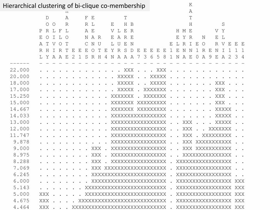
Hierarchical clustering of bi-clique co-membership
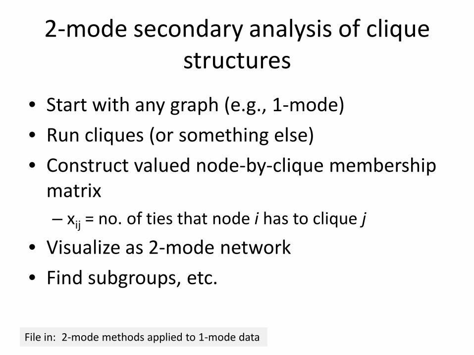
2-mode secondary analysis of clique structures
• Start with any graph (e.g., 1-mode)
• Run cliques (or something else)
• Construct valued node-by-clique membership matrix– xij = no. of ties that node i has to clique j
• Visualize as 2-mode network
• Find subgroups, etc.
File in: 2-mode methods applied to 1-mode data
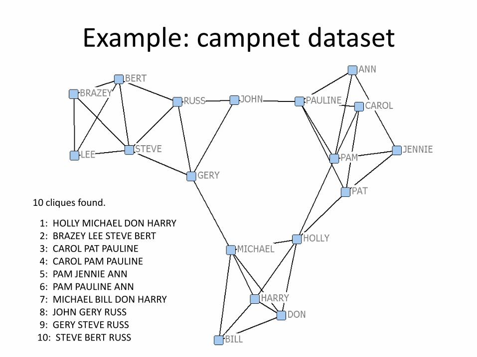
Example: campnet dataset
10 cliques found.
1: HOLLY MICHAEL DON HARRY2: BRAZEY LEE STEVE BERT3: CAROL PAT PAULINE4: CAROL PAM PAULINE5: PAM JENNIE ANN6: PAM PAULINE ANN7: MICHAEL BILL DON HARRY8: JOHN GERY RUSS9: GERY STEVE RUSS10: STEVE BERT RUSS
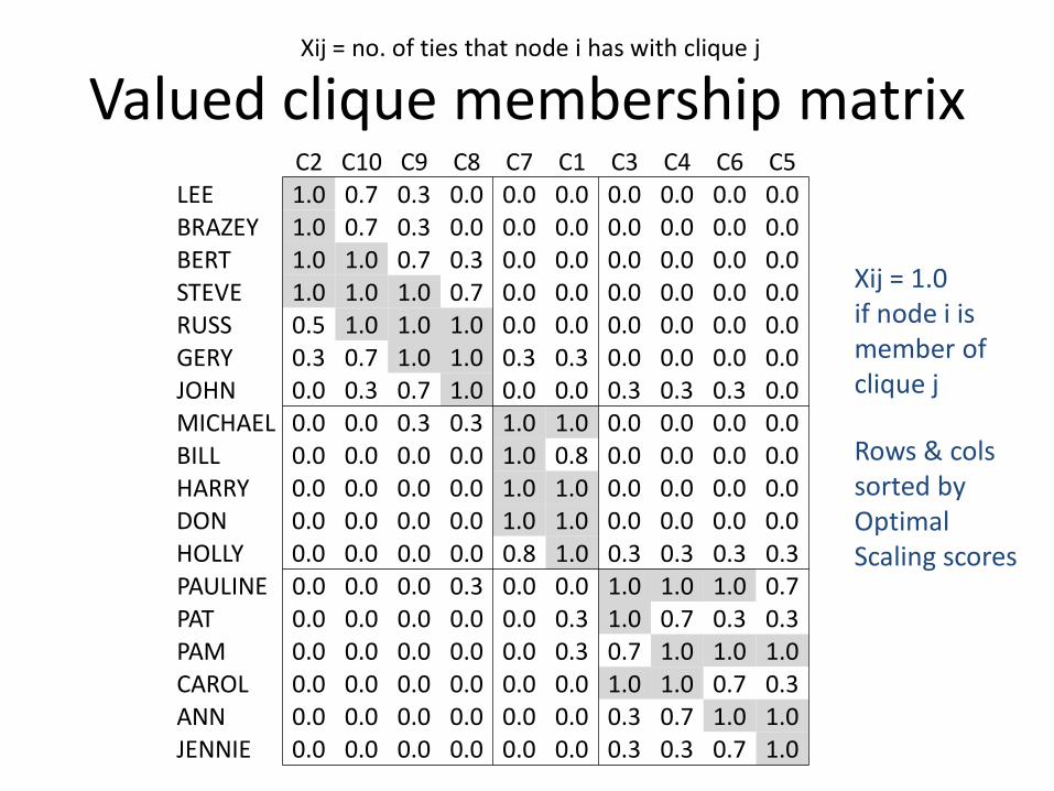
Valued clique membership matrixXij = no. of ties that node i has with clique j
Xij = 1.0 if node i is member of clique j
C2 C10 C9 C8 C7 C1 C3 C4 C6 C5LEE 1.0 0.7 0.3 0.0 0.0 0.0 0.0 0.0 0.0 0.0BRAZEY 1.0 0.7 0.3 0.0 0.0 0.0 0.0 0.0 0.0 0.0BERT 1.0 1.0 0.7 0.3 0.0 0.0 0.0 0.0 0.0 0.0STEVE 1.0 1.0 1.0 0.7 0.0 0.0 0.0 0.0 0.0 0.0RUSS 0.5 1.0 1.0 1.0 0.0 0.0 0.0 0.0 0.0 0.0GERY 0.3 0.7 1.0 1.0 0.3 0.3 0.0 0.0 0.0 0.0JOHN 0.0 0.3 0.7 1.0 0.0 0.0 0.3 0.3 0.3 0.0MICHAEL 0.0 0.0 0.3 0.3 1.0 1.0 0.0 0.0 0.0 0.0BILL 0.0 0.0 0.0 0.0 1.0 0.8 0.0 0.0 0.0 0.0HARRY 0.0 0.0 0.0 0.0 1.0 1.0 0.0 0.0 0.0 0.0DON 0.0 0.0 0.0 0.0 1.0 1.0 0.0 0.0 0.0 0.0HOLLY 0.0 0.0 0.0 0.0 0.8 1.0 0.3 0.3 0.3 0.3PAULINE 0.0 0.0 0.0 0.3 0.0 0.0 1.0 1.0 1.0 0.7PAT 0.0 0.0 0.0 0.0 0.0 0.3 1.0 0.7 0.3 0.3PAM 0.0 0.0 0.0 0.0 0.0 0.3 0.7 1.0 1.0 1.0CAROL 0.0 0.0 0.0 0.0 0.0 0.0 1.0 1.0 0.7 0.3ANN 0.0 0.0 0.0 0.0 0.0 0.0 0.3 0.7 1.0 1.0JENNIE 0.0 0.0 0.0 0.0 0.0 0.0 0.3 0.3 0.7 1.0
Rows & cols sorted by Optimal Scaling scores
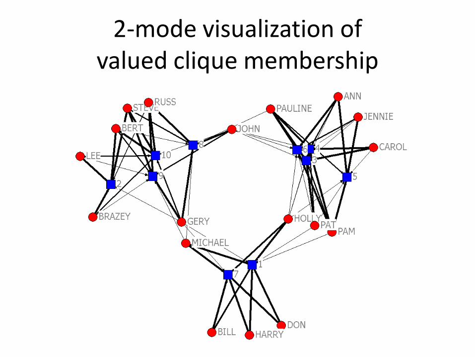
2-mode visualization of valued clique membership
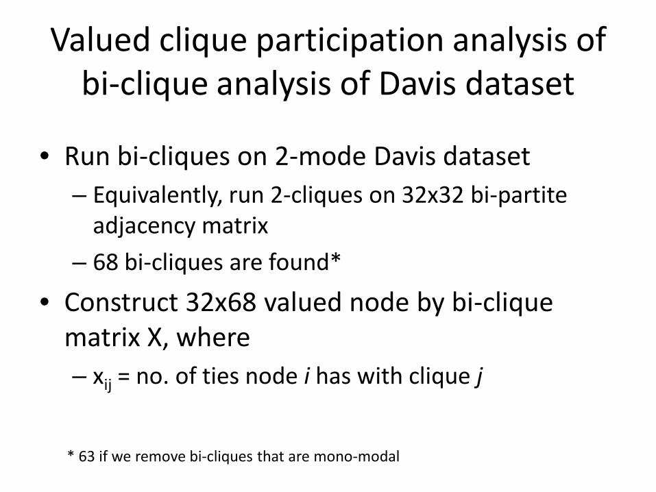
Valued clique participation analysis of bi-clique analysis of Davis dataset
• Run bi-cliques on 2-mode Davis dataset– Equivalently, run 2-cliques on 32x32 bi-partite
adjacency matrix
– 68 bi-cliques are found*
• Construct 32x68 valued node by bi-clique matrix X, where – xij = no. of ties node i has with clique j
* 63 if we remove bi-cliques that are mono-modal
Bi-clique analysis of Davis dataset
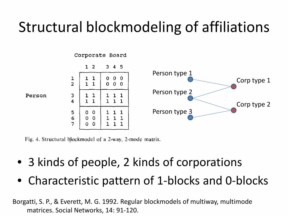
Structural blockmodeling of affiliations
• 3 kinds of people, 2 kinds of corporations
• Characteristic pattern of 1-blocks and 0-blocks
Corp type 1
Corp type 2
Person type 1
Person type 3
Person type 2
Borgatti, S. P., & Everett, M. G. 1992. Regular blockmodels of multiway, multimode matrices. Social Networks, 14: 91-120.
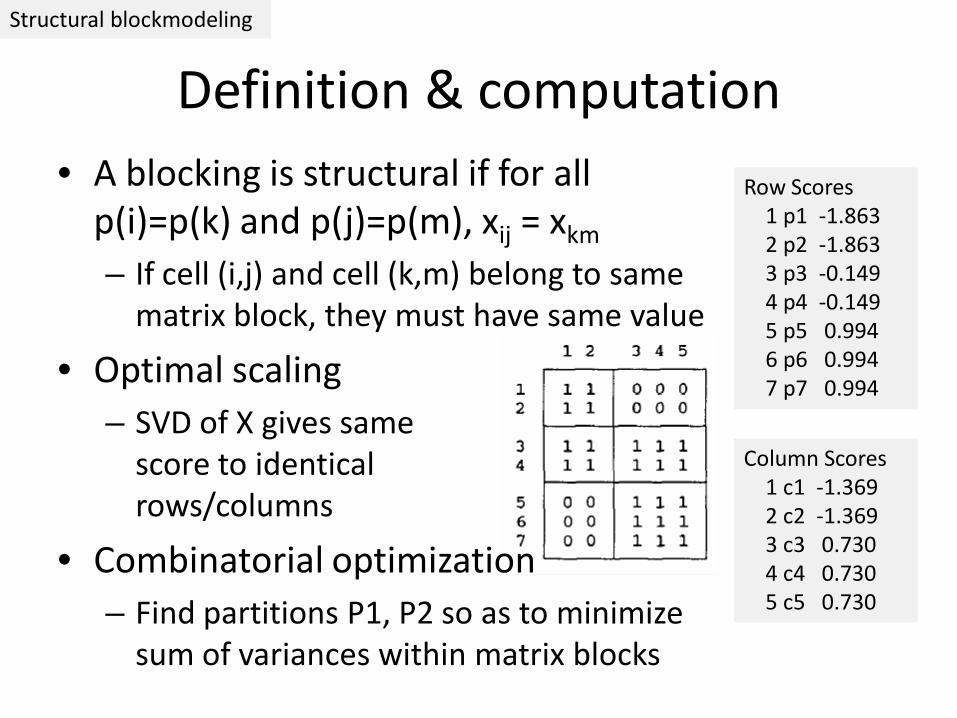
• A blocking is structural if for all p(i)=p(k) and p(j)=p(m), xij = xkm
– If cell (i,j) and cell (k,m) belong to same matrix block, they must have same value
• Optimal scaling – SVD of X gives same
score to identical rows/columns
• Combinatorial optimization– Find partitions P1, P2 so as to minimize
sum of variances within matrix blocks
Definition & computation
Row Scores1 p1 -1.8632 p2 -1.8633 p3 -0.1494 p4 -0.1495 p5 0.9946 p6 0.9947 p7 0.994
Column Scores1 c1 -1.3692 c2 -1.3693 c3 0.7304 c4 0.7305 c5 0.730
Structural blockmodeling
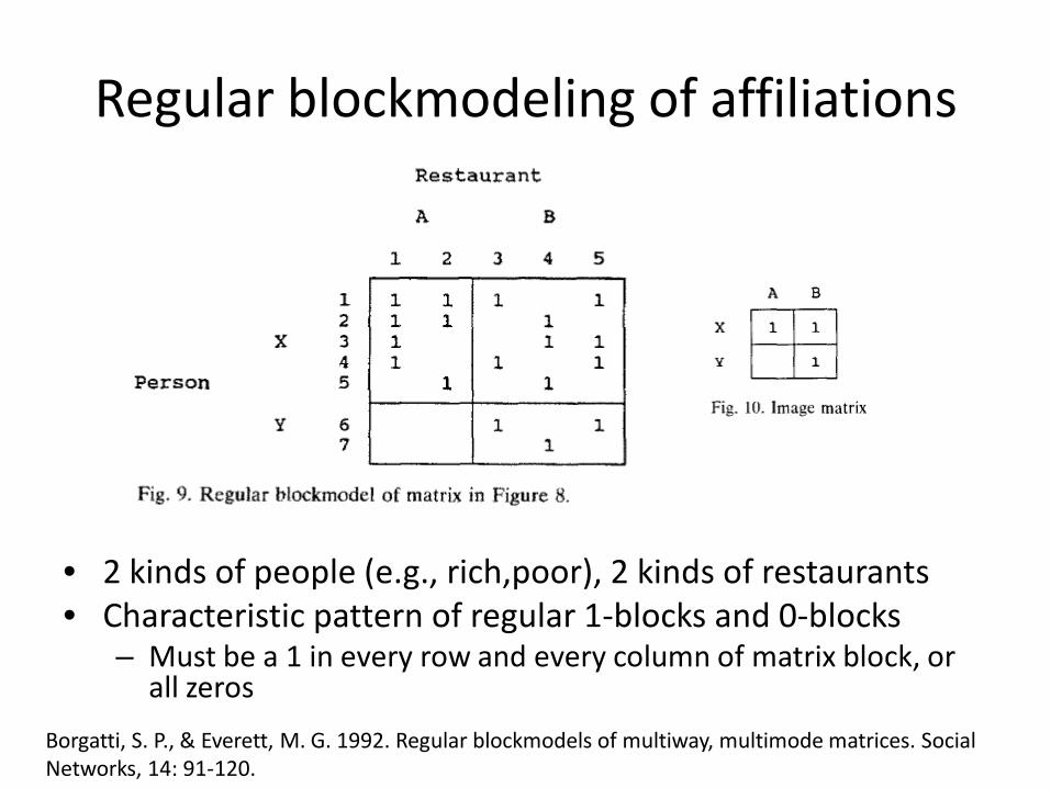
Regular blockmodeling of affiliations
• 2 kinds of people (e.g., rich,poor), 2 kinds of restaurants• Characteristic pattern of regular 1-blocks and 0-blocks
– Must be a 1 in every row and every column of matrix block, or all zeros
Borgatti, S. P., & Everett, M. G. 1992. Regular blockmodels of multiway, multimode matrices. Social Networks, 14: 91-120.
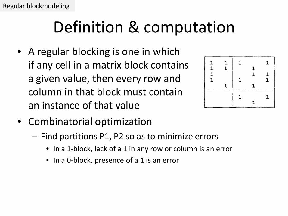
• A regular blocking is one in whichif any cell in a matrix block contains a given value, then every row and column in that block must contain an instance of that value
• Combinatorial optimization– Find partitions P1, P2 so as to minimize errors
• In a 1-block, lack of a 1 in any row or column is an error
• In a 0-block, presence of a 1 is an error
Definition & computationRegular blockmodeling

Side note: regular blockmodels of valued multi-mode matrices
• In an adj matrix, if we recode nulls to 2s and apply this definition of regular equiv, the resulting blockmodel will hold for the complement of the graph

FUTURE DIRECTIONS, APPLICATIONS ETC
Section 3
Under-developed areas
• Trajectories– e.g., careers
• Movement of actors through a resource or achievement space
• Relational algebras
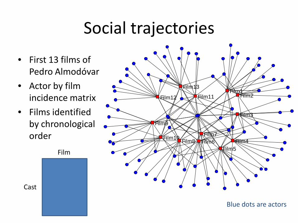
Film1
Film10
Film11Film12
Film13
Film2
Film3
Film4Film5
Film6Film7
Film8
Film9
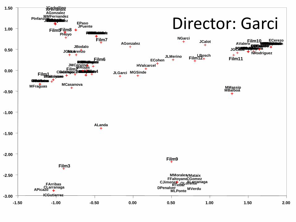
• First 13 films of Pedro Almodóvar
• Actor by film incidence matrix
• Films identified by chronological order
Social trajectories
Blue dots are actors
Cast
Film
Social Trajectories
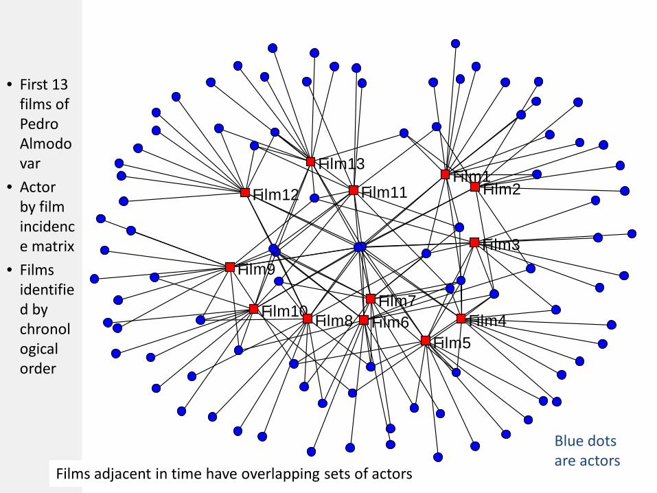
Film1
Film10
Film11Film12
Film13
Film2
Film3
Film4Film5
Film6Film7
Film8
Film9
• First 13 films of Pedro Almodovar
• Actor by film incidence matrix
• Films identified by chronological order
Films adjacent in time have overlapping sets of actors
Blue dots are actors
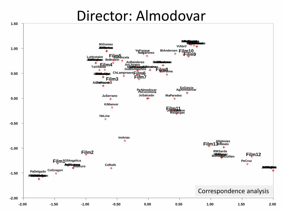
Director: Almodovar
-2.00
-1.50
-1.00
-0.50
0.00
0.50
1.00
1.50
-2.00 -1.50 -1.00 -0.50 0.00 0.50 1.00 1.50 2.00
ALFernandez
AVGomez
AfBeato
AgAlcazar
AgAlmodovar
AlaskaPegam
AlIglesias
AlAngulo
AlCasanovaAlMayoAnLizaranAnAlonso
AnSantana
AALopez
AnMolina
ASJuan
AnBanderasAnLlorens
AsSerna
AuGirard
BeBonezi
BiAndersen
CaPena
CaElias
CaMaura
CeRoth
ChLampreave
CoGregori
CrMarcos
CrPascual
EnMorricone
EnPosner
EsGarcia
EsRambal
EuPoncela
EvCobo
EvSilvaFeRotaeta
FeAtkine
FFGomezFeGuillen
FeVivancoFrNeri
FrFemenias
GoSuarez
GuMontesinos
HeLine
ImArias
JaBardem
JeFerrero
JLAlcaine
JoSalcedo
JoSancho
JuEchanove
JuMArtinez
JuSerrano
KiManver
LiRabal
LiCanalejas
LoCardonaLoLeonLuBriales
LuCalvo
LuHostalot
MAPCAmpos
MaZarzo
MaVargas
MaVelasco
MaCarillo
maBarranco
MaParedes
MaMuro
MaOWisiedo
MiRuben
MiGomez
MiMolinaMGRomero
NaMartinez
OfAngelica
OGAlaskaPaPochPaDelgado
PeAlmodovar
PeCruz
PeCoromina
PeCoyote
Pibardem
RMSarda
RdPalma
RySakamotoSaLajusticia
TaVillalba
VeForqueViAbril
Film13
Film12
Film11
Film10Film9
Film8Film7Film6
Film5
Film4
Film3
Film2
Film1
Correspondence analysis
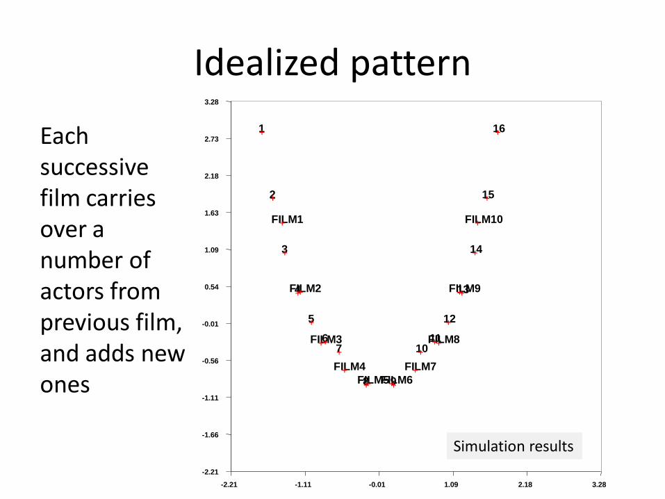
Idealized pattern
Each successive film carries over a number of actors from previous film, and adds new ones
-2.21
-1.66
-1.11
-0.56
-0.01
0.54
1.09
1.63
2.18
2.73
3.28
-2.21 -1.11 -0.01 1.09 2.18 3.28
1
2
3
4
5
67
8 9
1011
12
13
14
15
16
FILM1
FILM2
FILM3
FILM4FILM5FILM6
FILM7
FILM8
FILM9
FILM10
Simulation results
-3.00
-2.50
-2.00
-1.50
-1.00
-0.50
0.00
0.50
1.00
1.50
-1.50 -1.00 -0.50 0.00 0.50 1.00 1.50 2.00
JLGarci
JGCabaLBosch
LMDelgadoVPanero
HValcarcel
RPCubero
MBalboa
MGSinde
FFGomezRAlonsoCGCuervoAGonzalezCCruzARozasFGuillen
FGuillenCuervoFPiquer
MMassip
JCarideJCarideFAlgora
ECohen
JCalotCGCondeAValero
NRodriguezJLMerino
MSampietroBSantanaEAsensiMEFloresNGarci
MRMartinezLdOrdunaDAguadoABSanchezRVillascastinACarbonellECerezo
FFaltoyanoALarranagaVMataix
DPenalverMLPonte MVerdu
CGomez
ALanda
CJimenez OLorenteRTebar
MRojas
MMorales
JGluck
CPorterJPachelbelALlorenteJPuente
TGimperaVVeraEHoyoPSerrador
MLorenzo
PHoyo
SAmonJCuetoSCanadaJMFernandezPInfanzon
JCarballino
AMarsillach
MCasanova
JBodalo
EPaso
VValverdePCalotESuarezRHernandezYRiosDSalcedo
MRellanRdPenagosAFernandezJMCervino
MMerchanteJYepesFBilbao
AFerrandisAGonzalez
MMFernandez
MTejadaMRellanRFraileFVidalMBlascoMoWisiedoEFornet
CLarranagaAPicazoICGutierrez
FArribas
JSacristanFFaltoyanoGCobosCRodriguez
AGameroSTortosaSAndreuHAlterioCCadenasBertaMFraguas
Film12 Film11
Film10
Film9
Film8
Film7
Film6
Film5
Film4
Film3
Film2Film1
Director: Garci
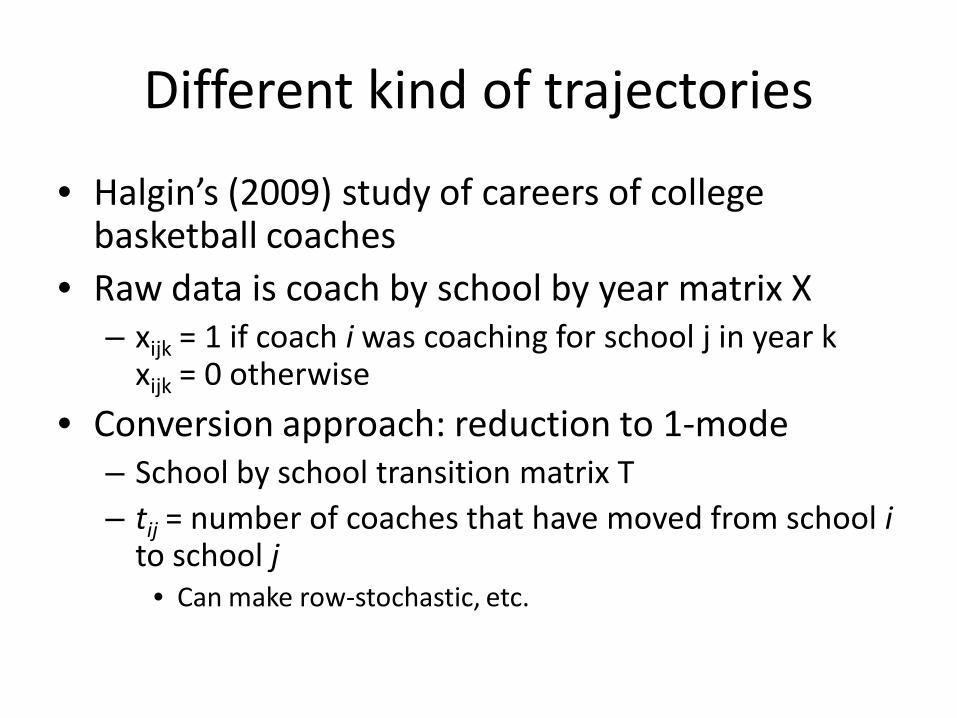
Different kind of trajectories
• Halgin’s (2009) study of careers of college basketball coaches
• Raw data is coach by school by year matrix X – xijk = 1 if coach i was coaching for school j in year k
xijk = 0 otherwise
• Conversion approach: reduction to 1-mode– School by school transition matrix T– tij = number of coaches that have moved from school i
to school j• Can make row-stochastic, etc.
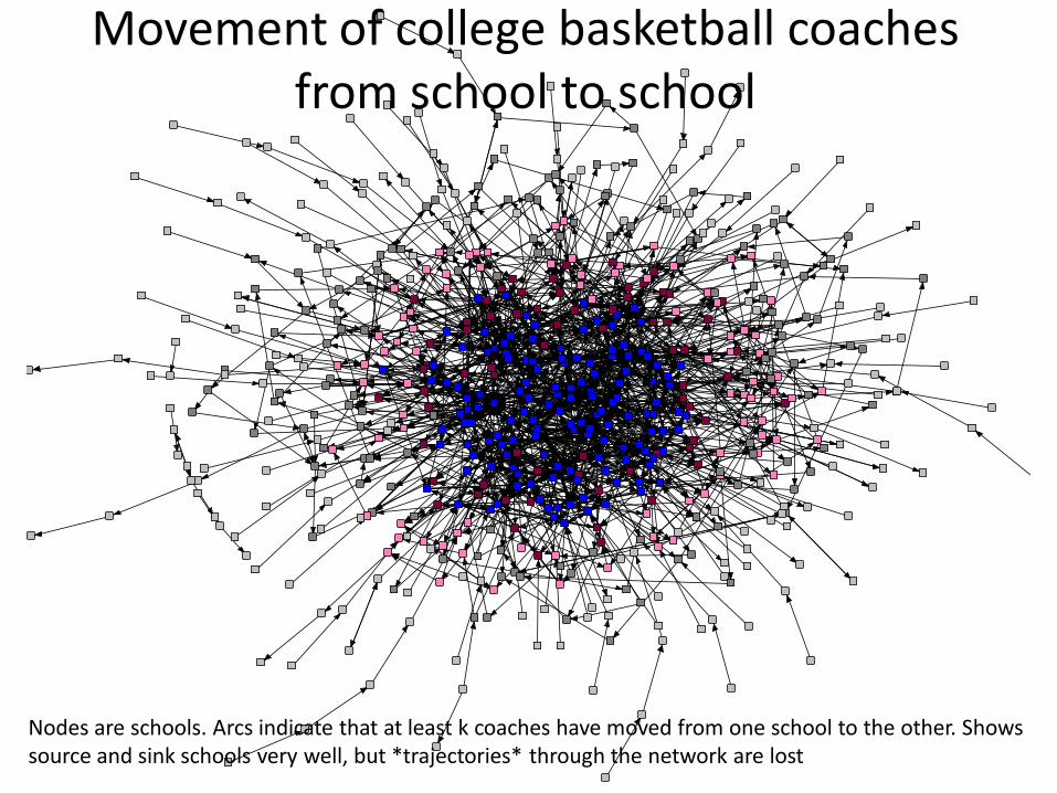
Movement of college basketball coaches from school to school
Nodes are schools. Arcs indicate that at least k coaches have moved from one school to the other. Shows source and sink schools very well, but *trajectories* through the network are lost
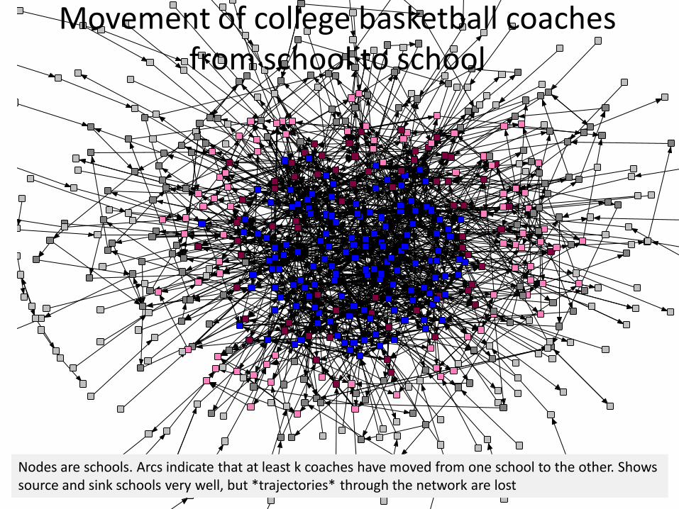
Movement of college basketball coaches from school to school
Nodes are schools. Arcs indicate that at least k coaches have moved from one school to the other. Shows source and sink schools very well, but *trajectories* through the network are lost
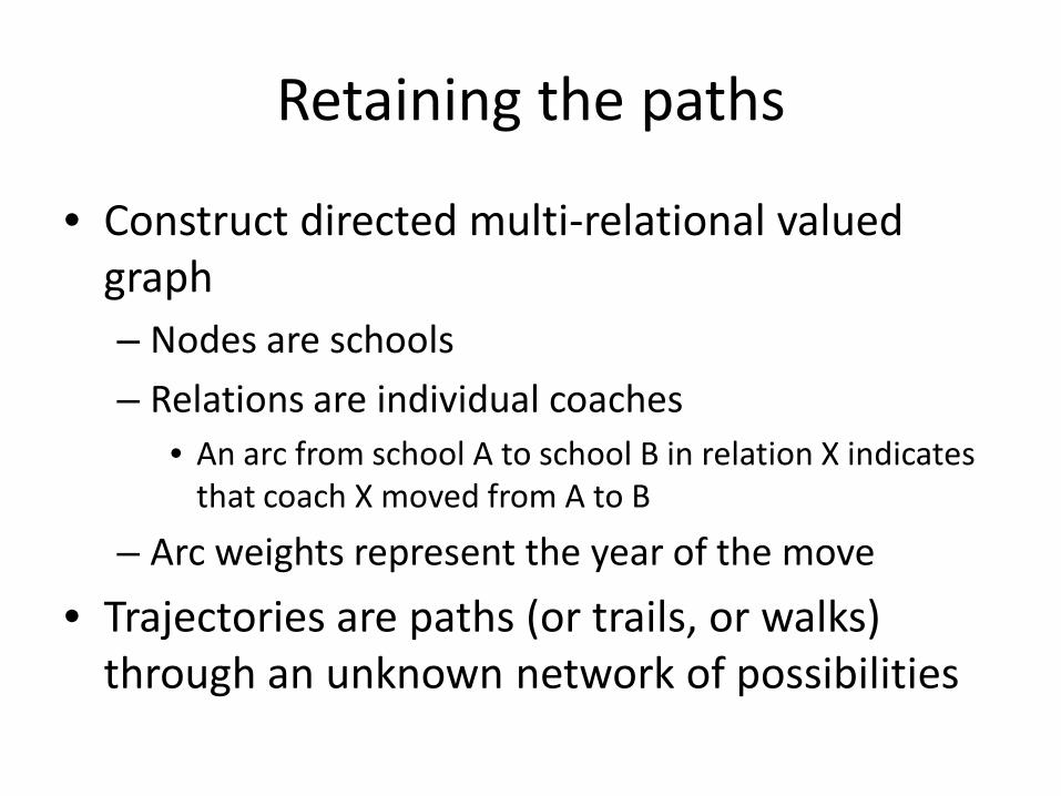
Retaining the paths
• Construct directed multi-relational valued graph– Nodes are schools
– Relations are individual coaches• An arc from school A to school B in relation X indicates
that coach X moved from A to B
– Arc weights represent the year of the move
• Trajectories are paths (or trails, or walks) through an unknown network of possibilities
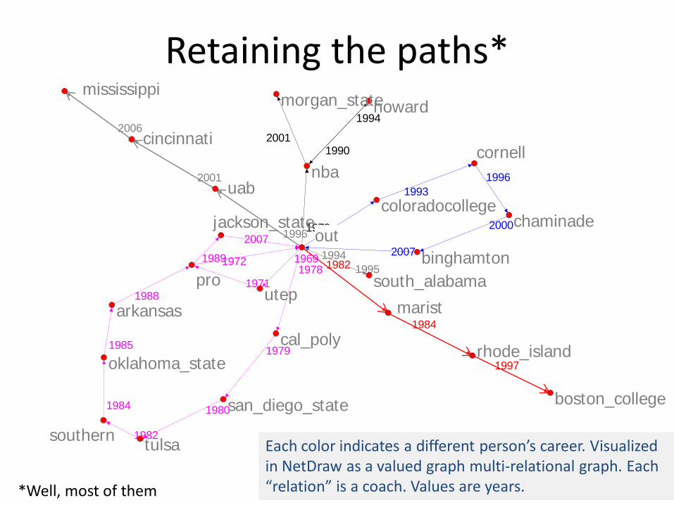
Retaining the paths*
1984
1997
19931996
2000
20071982
19881979
1994
1996
19691978
19902001
1994
1995
2001
2006
1971
19721989
1979
1980
1982
1984
1985
1988
2007
marist
rhode_island
boston_college
coloradocollege
cornell
chaminade
binghamtonout
nba
howardmorgan_state
south_alabama
uab
cincinnati
mississippi
uteppro
cal_poly
san_diego_state
tulsasouthern
oklahoma_state
arkansas
jackson_state
Each color indicates a different person’s career. Visualized in NetDraw as a valued graph multi-relational graph. Each “relation” is a coach. Values are years.*Well, most of them
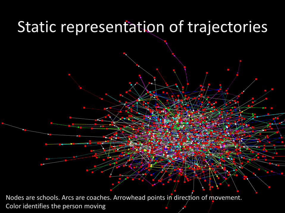
Nodes are schools. Arcs are coaches. Arrowhead points in direction of movement. Color identifies the person moving
Static representation of trajectories
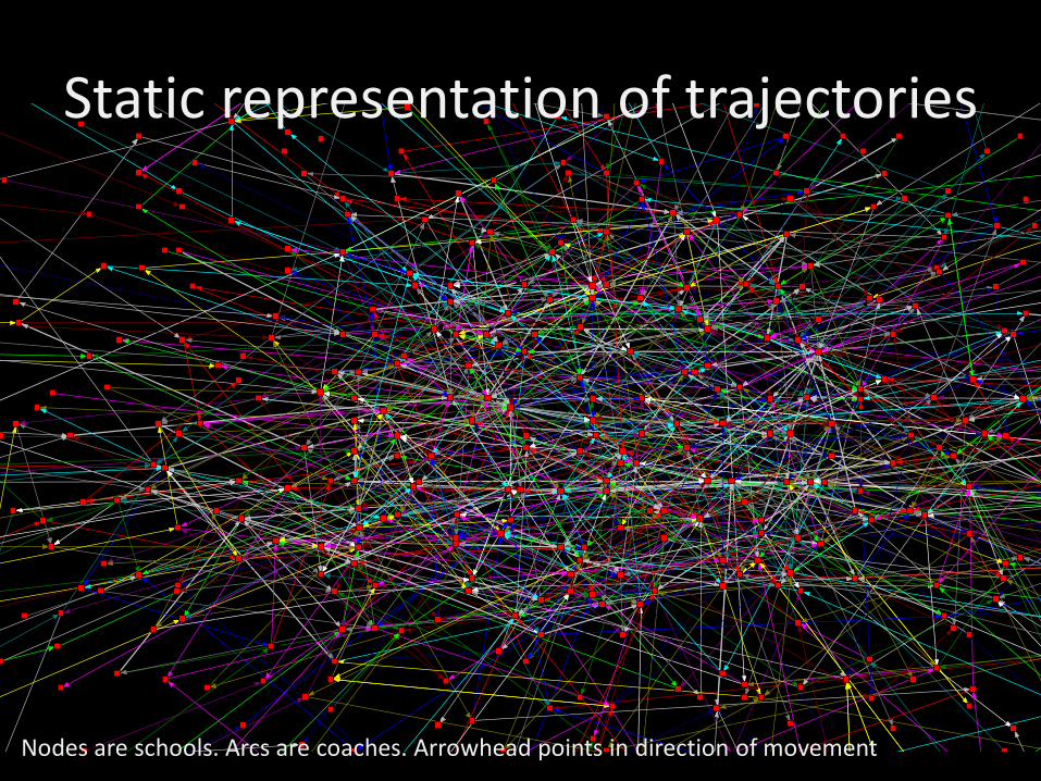
Nodes are schools. Arcs are coaches. Arrowhead points in direction of movement
Static representation of trajectories
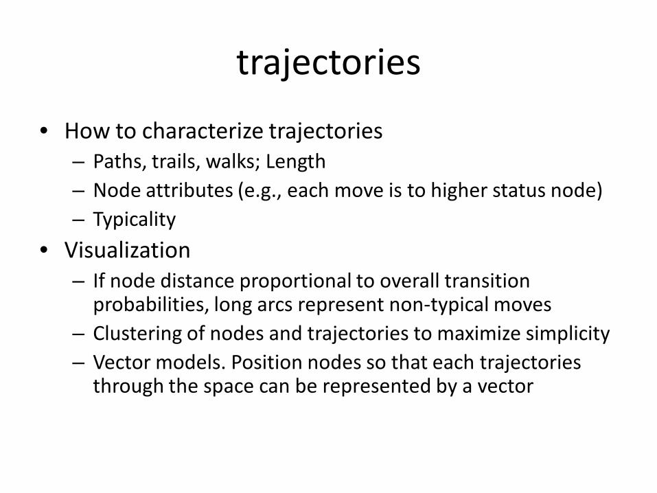
trajectories
• How to characterize trajectories– Paths, trails, walks; Length– Node attributes (e.g., each move is to higher status node)– Typicality
• Visualization– If node distance proportional to overall transition
probabilities, long arcs represent non-typical moves– Clustering of nodes and trajectories to maximize simplicity– Vector models. Position nodes so that each trajectories
through the space can be represented by a vector
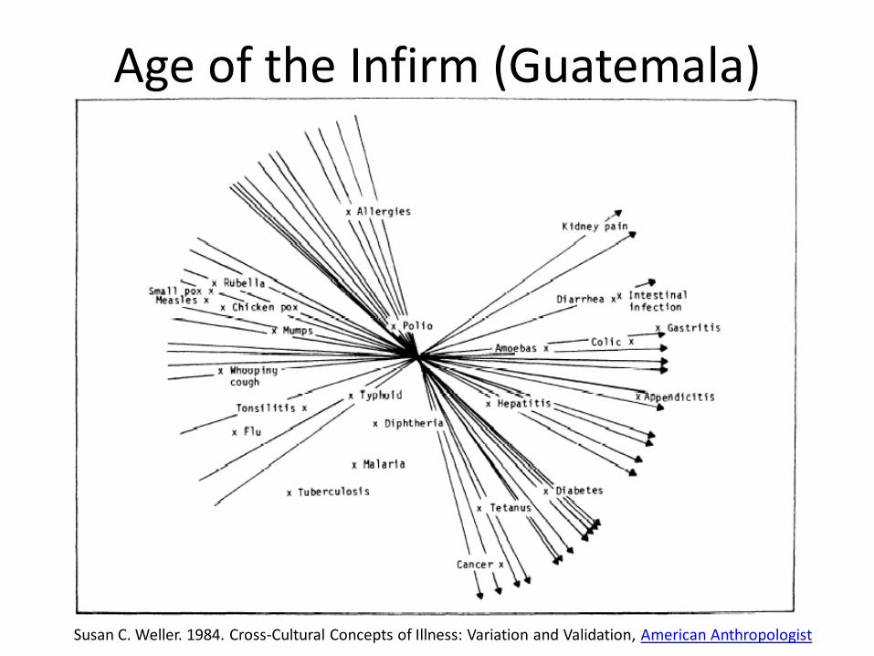
Age of the Infirm (Guatemala)
Susan C. Weller. 1984. Cross-Cultural Concepts of Illness: Variation and Validation, American Anthropologist
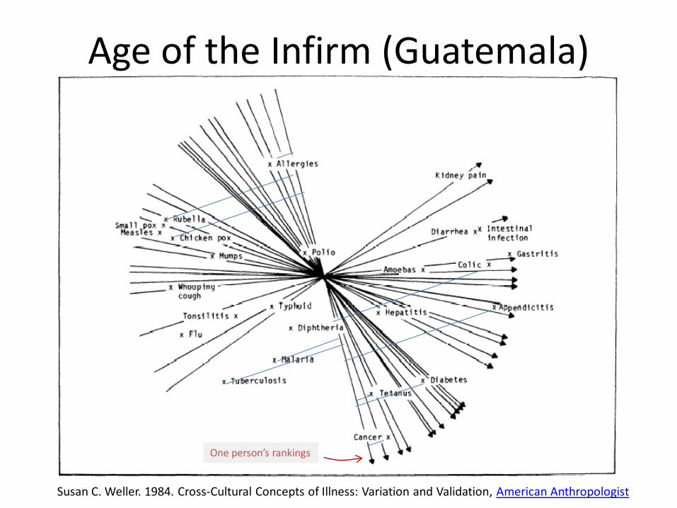
Age of the Infirm (Guatemala)
Susan C. Weller. 1984. Cross-Cultural Concepts of Illness: Variation and Validation, American Anthropologist
One person’s rankings
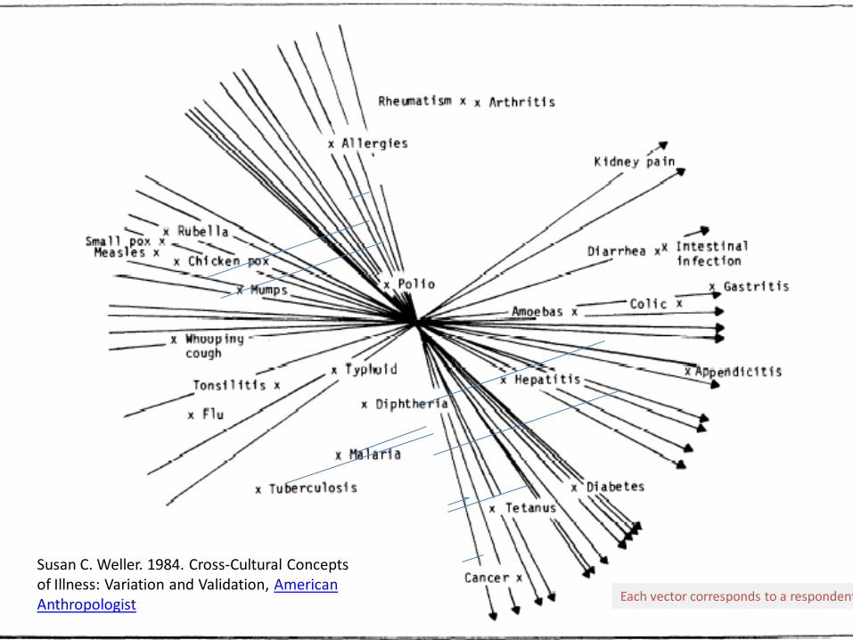
Age of the Infirm (Guatemala)
Susan C. Weller. 1984. Cross-Cultural Concepts of Illness: Variation and Validation, American Anthropologist Each vector corresponds to a respondent
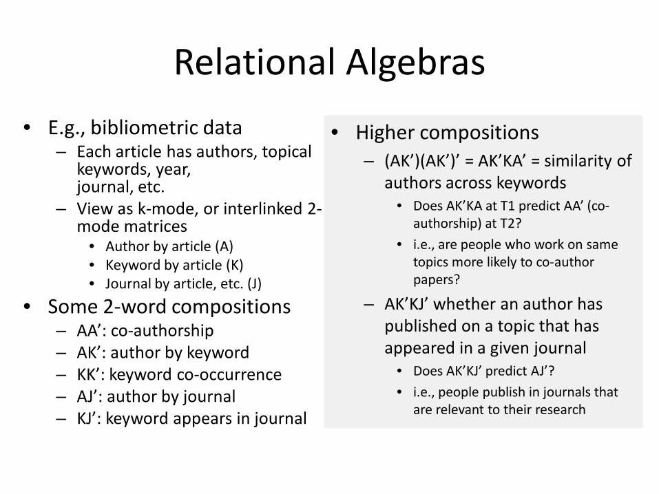
Relational Algebras
• E.g., bibliometric data– Each article has authors, topical
keywords, year, journal, etc.
– View as k-mode, or interlinked 2-mode matrices
• Author by article (A)• Keyword by article (K)• Journal by article, etc. (J)
• Some 2-word compositions– AA’: co-authorship– AK’: author by keyword– KK’: keyword co-occurrence– AJ’: author by journal– KJ’: keyword appears in journal
• Higher compositions– (AK’)(AK’)’ = AK’KA’ = similarity of
authors across keywords• Does AK’KA at T1 predict AA’ (co-
authorship) at T2?
• i.e., are people who work on same topics more likely to co-author papers?
– AK’KJ’ whether an author has published on a topic that has appeared in a given journal
• Does AK’KJ’ predict AJ’?
• i.e., people publish in journals that are relevant to their research
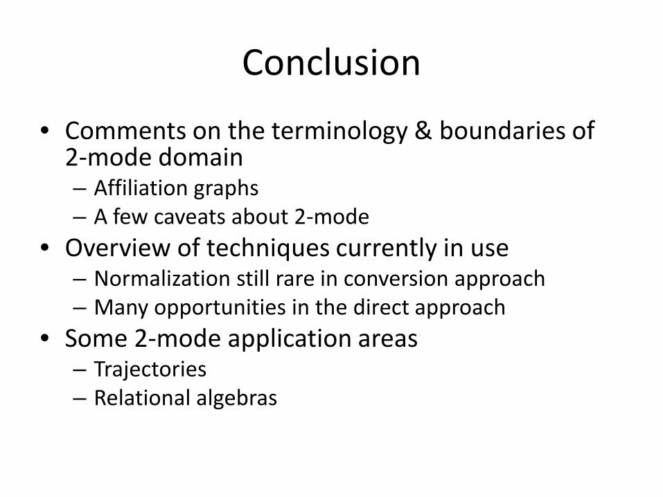
Conclusion
• Comments on the terminology & boundaries of 2-mode domain– Affiliation graphs– A few caveats about 2-mode
• Overview of techniques currently in use– Normalization still rare in conversion approach– Many opportunities in the direct approach
• Some 2-mode application areas– Trajectories– Relational algebras

end.
Better get to our lunch before someone else does …