Embed Size (px)
Citation preview
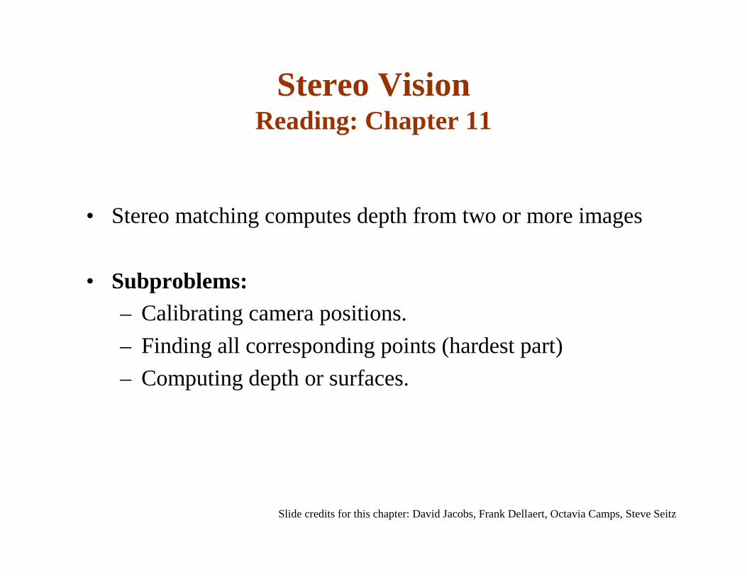
Stereo VisionReading: Chapter 11
• Stereo matching computes depth from two or more images
• Subproblems:– Calibrating camera positions.
– Finding all corresponding points (hardest part)
– Computing depth or surfaces.
Slide credits for this chapter: David Jacobs, Frank Dellaert, Octavia Camps, Steve Seitz

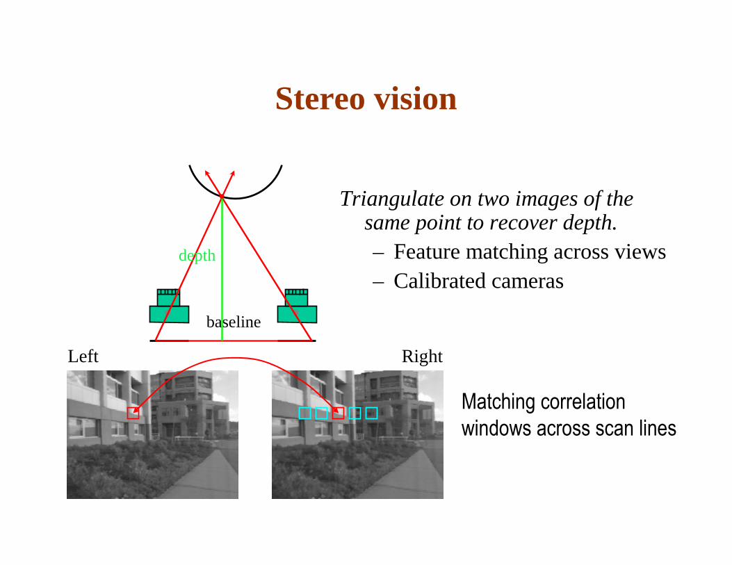
Stereo vision
Triangulate on two images of the same point to recover depth.– Feature matching across views– Calibrated cameras
Left Right
baseline
Matching correlation
windows across scan lines
depth
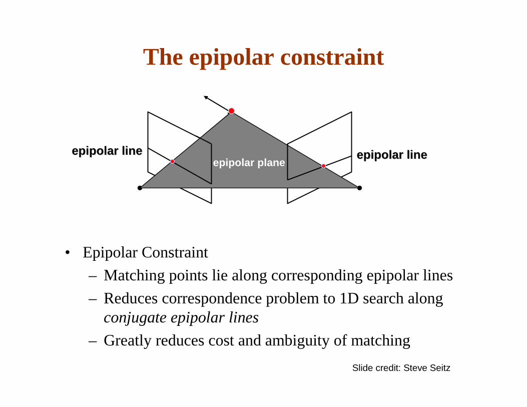
The epipolar constraint
• Epipolar Constraint
– Matching points lie along corresponding epipolar lines
– Reduces correspondence problem to 1D search along conjugate epipolar lines
– Greatly reduces cost and ambiguity of matching
epipolar planeepipolar lineepipolar lineepipolar lineepipolar line
Slide credit: Steve Seitz

Simplest Case: Rectified Images
• Image planes of cameras are parallel.
• Focal points are at same height.
• Focal lengths same.
• Then, epipolar lines fall along the horizontal scan lines of the images
• We will assume images have been rectified so that epipolar lines correspond to scan lines
– Simplifies algorithms
– Improves efficiency

We can always achieve this geometry with image rectification
• Image Reprojection– reproject image planes onto common
plane parallel to line between optical centers
• Notice, only focal point of camera really matters
(Seitz)

Basic Stereo Derivations
PL = (X,Y,Z)OL
x
y
z (uL,vL)
OR
x
y
z
(uR,vR)
base
line B
Disparity:
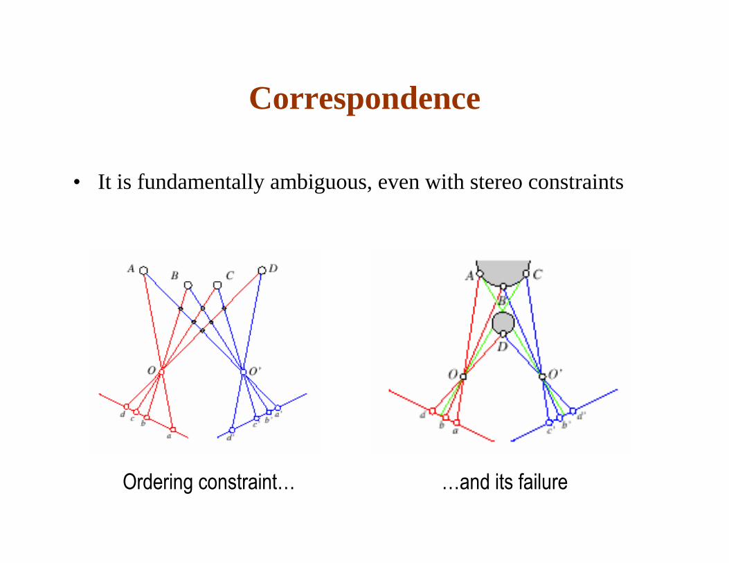
Correspondence
• It is fundamentally ambiguous, even with stereo constraints
Ordering constraint… …and its failure
Correspondence: What should we match?
• Objects?
• Edges?
• Pixels?
• Collections of pixels?

Julesz: showed that recognition is not needed for stereo.
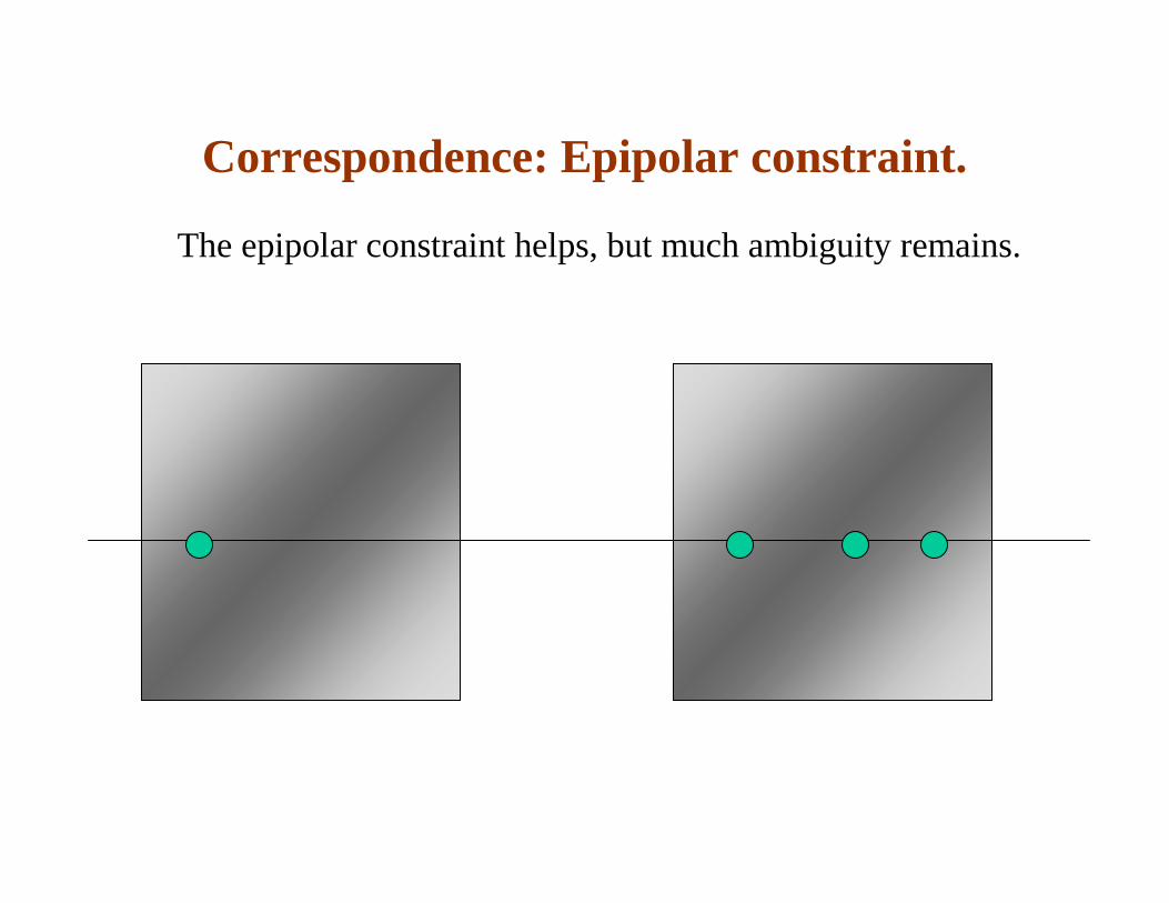
Correspondence: Epipolar constraint.
The epipolar constraint helps, but much ambiguity remains.

Correspondence: Photometric constraint
• Same world point has same intensity in both images.
– True for Lambertian surfaces
• A Lambertian surface has a brightness that is independent of viewing angle
– Violations:
• Noise
• Specularity
• Non-Lambertian materials
• Pixels that contain multiple surfaces

Pixel matching
For each epipolar lineFor each pixel in the left image
• compare with every pixel on same epipolar line in right image
• pick pixel with minimum match cost
This leaves too much ambiguity, so:
Improvement: match windows(Seitz)
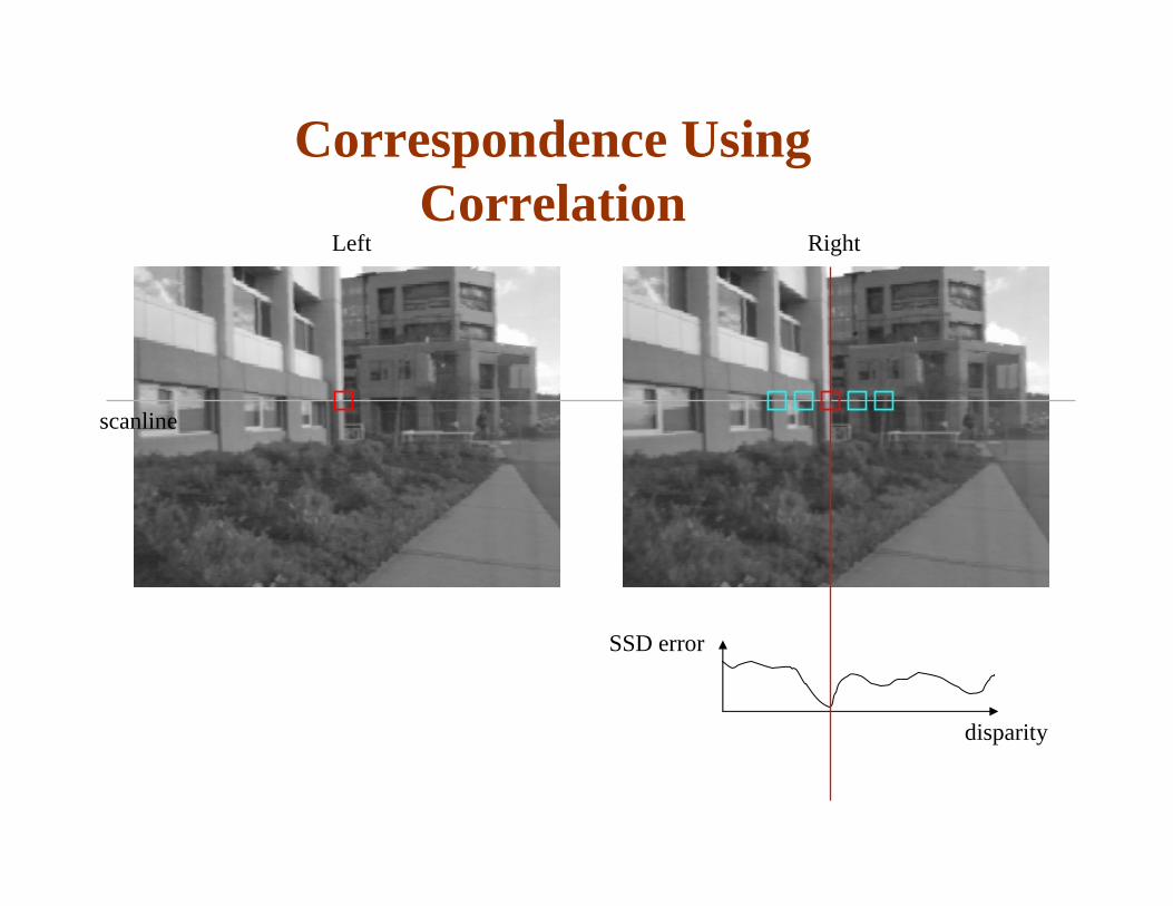
Correspondence Using Correlation
SSD error
disparity
Left Right
scanline

Sum of Squared (Pixel) Differences
Left Right
Lw Rw
LI RI
∑∈
−−=
+≤≤−+≤≤−=
),(),(
2
2222
)],(),([),,(
:disparity offunction a as differenceintensity themeasurescost SSD The
},|,{),(
:function window thedefine We
pixels. of windowsby ingcorrespond are and
yxWvuRLr
mmmmm
RL
m
vduIvuIdyxC
yvyxuxvuyxW
mmww
LwRw
),( LL yx ),( LL ydx −
m
m

Image Normalization
• Even when the cameras are identical models, there can be differences in gain and sensitivity.
• For these reason and more, it is a good idea to normalize the pixels in each window:
pixel Normalized ),(
),(ˆ
magnitude Window )],([
pixel Average ),(
),(
),(),(
2
),(
),(),(),(
1
yxW
yxWvuyxW
yxWvuyxW
m
mm
m
m
II
IyxIyxI
vuII
vuII
−−=
=
=
∑
∑
∈
∈

Images as Vectors
Left Right
LwRw
m
m
Lw
Lw
row 1
row 2
row 3
m
m
m
“Unwrap”image to form vector, using raster scan order
Each window is a vectorin an m2 dimensionalvector space.Normalization makesthem unit length.
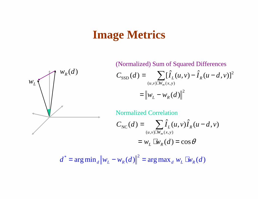
Image Metrics
Lw)(dwR
2
),(),(
2SSD
)(
)],(ˆ),(ˆ[)(
dww
vduIvuIdC
RL
yxWvuRL
m
−=
−−= ∑∈
(Normalized) Sum of Squared Differences
Normalized Correlation
θcos)(
),(ˆ),(ˆ)(),(),(
NC
=⋅=
−= ∑∈
dww
vduIvuIdC
RL
yxWvuRL
m
)(maxarg)(minarg2* dwwdwwd RLdRLd ⋅=−=

Stereo Results
Images courtesy of Point Grey Research

Window size
W = 3 W = 20
• Effect of window size
• Some approaches have been developed to use an adaptive window size (try multiple sizes and select best match)
(Seitz)
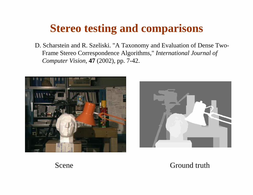
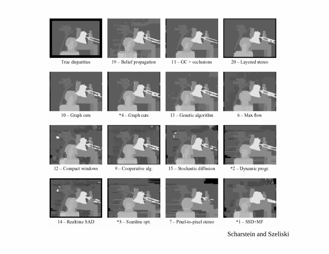
Stereo testing and comparisons
Ground truthScene
D. Scharstein and R. Szeliski. "A Taxonomy and Evaluation of Dense Two-Frame Stereo Correspondence Algorithms," International Journal of Computer Vision, 47 (2002), pp. 7-42.

Scharstein and Szeliski
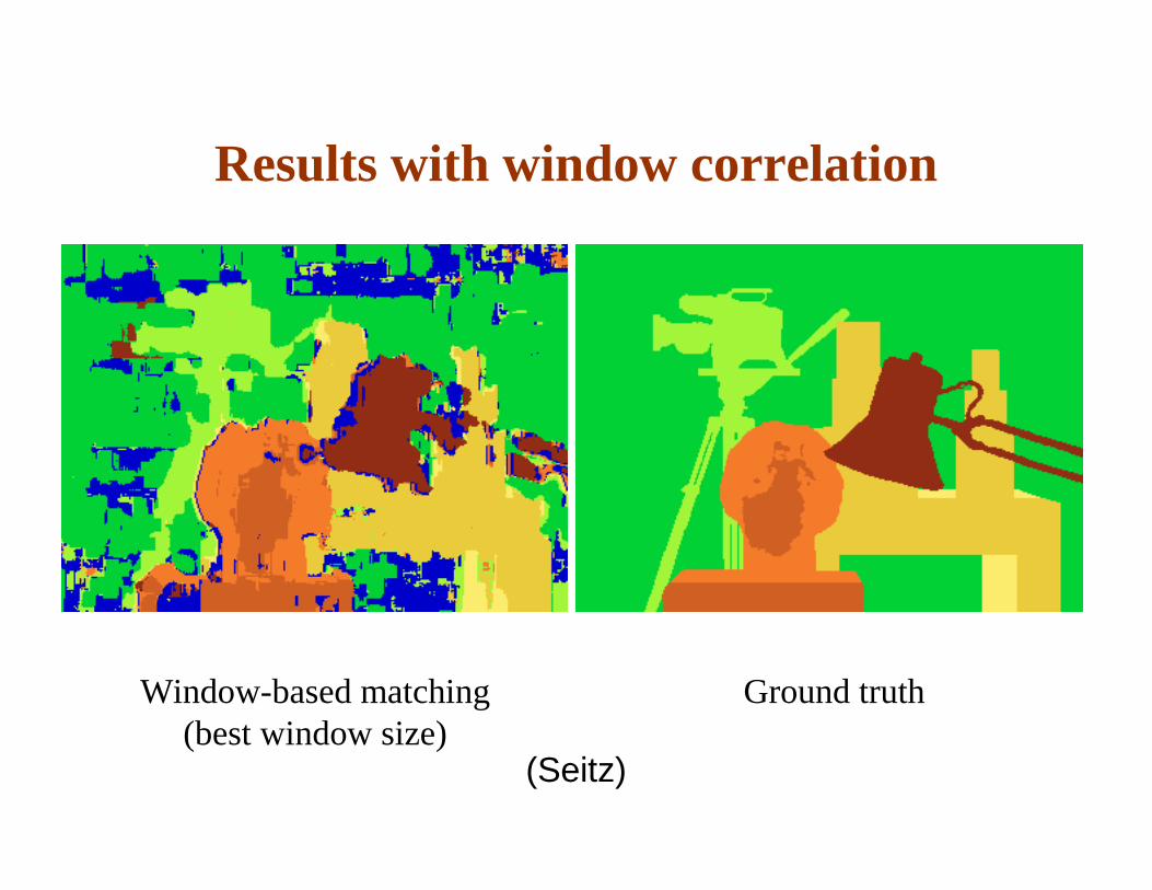
Results with window correlation
Window-based matching(best window size)
Ground truth
(Seitz)
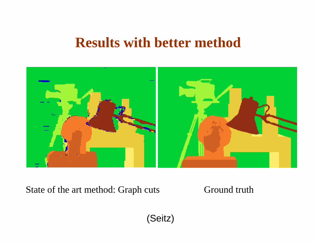
Results with better method
State of the art method: Graph cuts Ground truth
(Seitz)
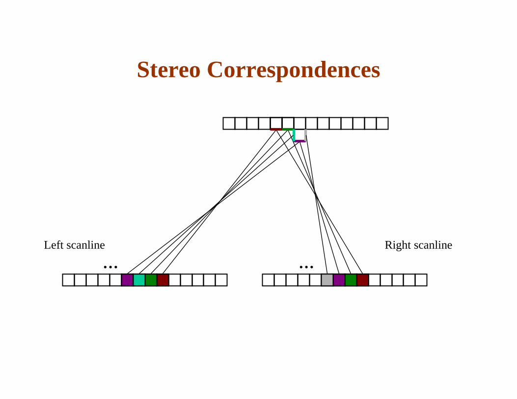
Stereo Correspondences
… …Left scanline Right scanline

Stereo Correspondences
… …Left scanline Right scanline
Match
Match
MatchOcclusion Disocclusion
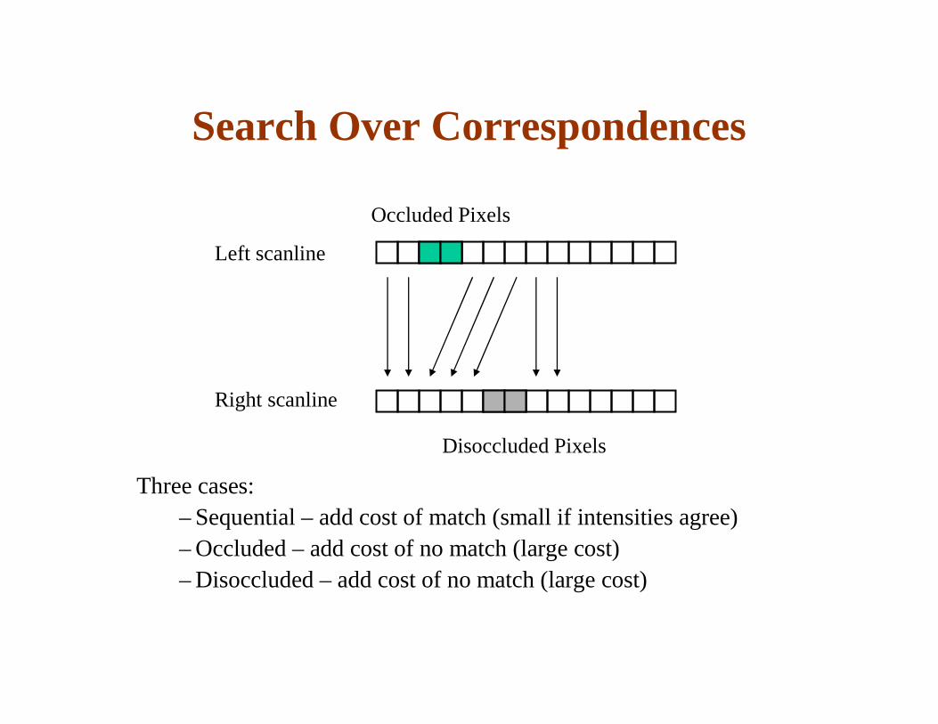
Search Over Correspondences
Three cases:– Sequential – add cost of match (small if intensities agree)– Occluded – add cost of no match (large cost)– Disoccluded – add cost of no match (large cost)
Left scanline
Right scanline
Occluded Pixels
Disoccluded Pixels
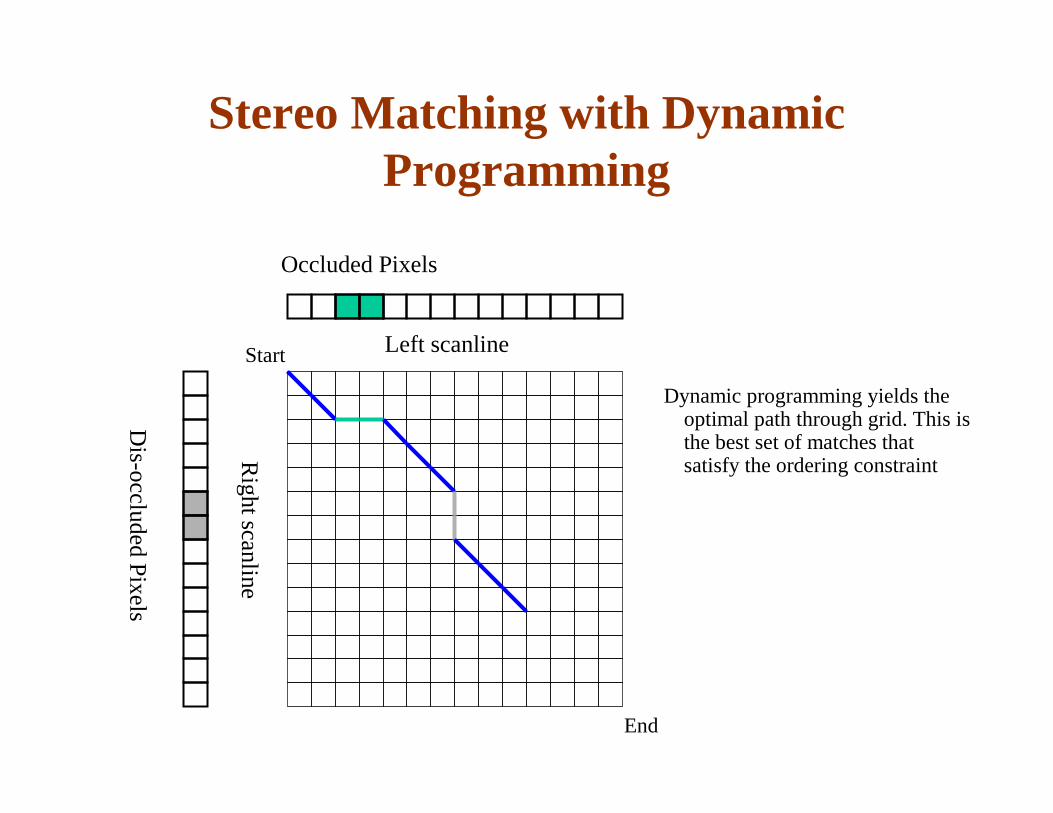
Stereo Matching with Dynamic Programming
Dynamic programming yields the optimal path through grid. This is the best set of matches that satisfy the ordering constraint
Occluded Pixels
Left scanline
Dis-occlude
d Pixe
ls
Right sca
nline
Start
End

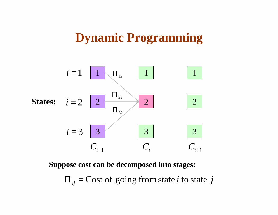
Dynamic Programming
• Efficient algorithm for solving sequential decision (optimal path) problems.
1
2
3
1
2
3
1
2
3
1=t 2=t 3=t
1=i
2=i
3=i
1
2
3
Tt =
…
How many paths through this trellis? T3
Dynamic Programming
1
2
3
1
2
3
1
2
3
1−tC tC 1+tC
12Π
22Π
32Π
Suppose cost can be decomposed into stages:
jiij state to state from going ofCost =Π
1=i
2=i
3=i
States:
Dynamic Programming
1
2
3
1
2
3
1
2
3
1−tC tC 1+tC
12Π
22Π
32Π
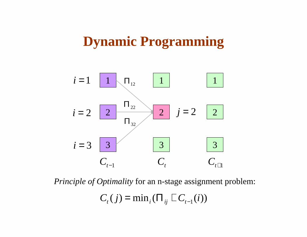
Principle of Optimality for an n-stage assignment problem:
))((min)( 1 iCjC tijit −+Π=
2=j
1=i
2=i
3=i
Dynamic Programming
1
2
3
1
2
3
1
2
3
1−tC tC 1+tC
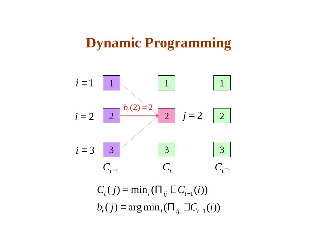
2)2( =tb
))((minarg)(
))((min)(
1
1
iCjb
iCjC
tijit
tijit
−
−
+Π=
+Π=
2=j
1=i
2=i
3=i
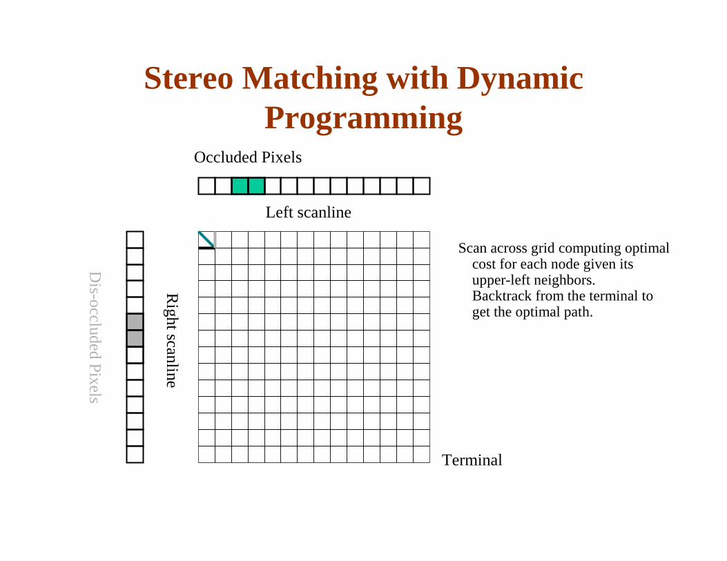
Stereo Matching with Dynamic Programming
Scan across grid computing optimal cost for each node given its upper-left neighbors.Backtrack from the terminal to get the optimal path.
Occluded Pixels
Left scanline
Dis-occlude
d Pixe
ls
Right sca
nline
Terminal

Stereo Matching with Dynamic Programming
Scan across grid computing optimal cost for each node given its upper-left neighbors.Backtrack from the terminal to get the optimal path.
Occluded Pixels
Left scanline
Dis-occlude
d Pixe
ls
Right sca
nline
Terminal
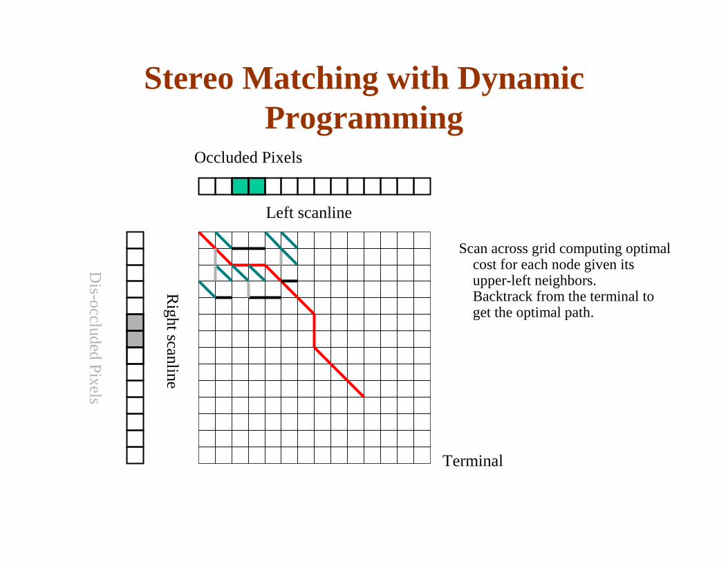
Stereo Matching with Dynamic Programming
Scan across grid computing optimal cost for each node given its upper-left neighbors.Backtrack from the terminal to get the optimal path.
Occluded Pixels
Left scanline
Dis-occlude
d Pixe
ls
Right sca
nline
Terminal
Scharstein and Szeliski

Segmentation-based Stereo
Hai Tao and Harpreet W. Sawhney
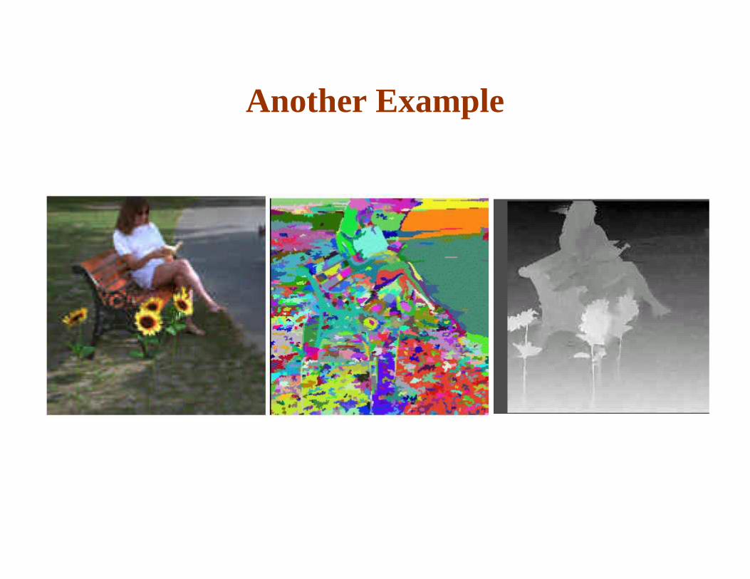
Another Example
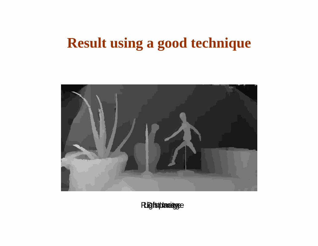
Result using a good technique
Right ImageLeft ImageDisparity
View Interpolation

Computing Correspondence
• Another approach is to match edges rather than windows of pixels:
• Which method is better?
– Edges tend to fail in dense texture (outdoors)
– Correlation tends to fail in smooth featureless areas

Summary of different stereo methods
• Constraints:– Geometry, epipolar constraint.– Photometric: Brightness constancy, only partly true.– Ordering: only partly true.– Smoothness of objects: only partly true.
• Algorithms: – What you compare: points, regions, features?
• How you optimize:– Local greedy matches.– 1D search.– 2D search.