Embed Size (px)
Citation preview
Stereo to Binaural Upmix Based on
Ambience Extraction
Sánchez Guzmán, Yeray
Curs 2018-2019
Director: Andrés Pérez López
GRAU EN ENGINYERIA DE SISTEMES AUDIOVISUALS
Treball de Fi de Grau
GRAU EN ENGINYERIA EN
xxxxxxxxxxxx
Stereo to Binaural Upmix Based on Ambience
Extraction
Yeray Sánchez Guzmán
TREBALL FI DE GRAU
Enginyeria en Sistemes Audiovisuals
ESCOLA SUPERIOR POLITÈCNICA UPF
2019
DIRECTOR DEL TREBALL
Andrés Pérez López

2

3
Dedicated to all those who have transmitted me the passion for learning as well as those
who have helped me to travel this path.


5
Acknowledgement
This project would not have been possible without the involvement of many people, so I
want to thank them all greatly.
First of all, my family, whose constant support throughout these years has given me the
opportunity to arrive this far. To my friends, with whom the degree has become more
enjoyable and in whose company I have been able to disconnect when I needed it.
Specially, I want to thank Fèlix for the help provided during the project, as well as for
gaining access to it.
And finally, to Andrés, for transmitting his passion for his field of study and guiding me
during these months.

6
7
Abstract
In this project we aim to create a 3D audio stereo upmix system with the purpose of
producing a more immersive listening experience. To do so, we use an approach which
segmentates the direct and ambience components of an audio file, using various factors
and assumptions. To create the immersive effect, we make use of Head Related Impulse
Responses (HRIRs) from both dummy heads and human subjects. The process output is
a stereo file containing a recreated binaural scene of the original stereo sound. Finally,
we perform a qualitative subjective evaluation of the different methods, based on listening
tests preferences.
Resumen En este Proyecto nuestro objetivo es el de crear una mezcla estéreo de audio 3D con el
fin de producir una mezcla más inmersiva. Para hacerlo, utilizamos un enfoque que
segmenta los componentes directos y ambientales de un archive de audio, utilizando
diversos factores y suposiciones. Para crear el efecto inmerso, utilizamos
respuestas impulsionales (HRIR) tanto de personas como de maniquíes. El resultado del
proceso es un archive estéreo que contiene una escena binaural recreada del sonido
estéreo original. Finalmente, realizamos una evaluación subjetiva cualitativa de los
diferentes métodos basándonos en las preferencias de las pruebas de audición.

9
Foreword
This TFG mainly focuses on Audio analysis, although it incorporates knowledge from
most of the topics seen throughout the degree such as programming, mathematics, and
signal processing.

11
Índex
Pàg.
Abstract................................................................................................................ 7
Foreword……...................................................................................................... 9
Figures Table….................................................................................................... 13
1.INTRODUCTION………..………................................................................... 15
1.1 Motivation and Objectives……….……………………………………… 15
2. RELATED WORK………………………………………………………….. 17
3. THEORETICAL CONCEPTS……………………......................................... 19
3.1 Introduction……….……………………………………………………... 19
3.2 Planes of the Head……….…….………………………………………… 19
3.3 Minimal Audible Angle…….……………………………………………. 20
3.4 Interaural Time Difference……….……………........................................ 21
a) Limits of the ITD...................................................................................... 23
3.5 Interaural Intensity Difference…………...……........................................ 24
a) Lateralization............................................................................................ 26
b) Cone of Confussion.................................................................................. 26
3.6 Binaural Audio…………………………...…………………………….... 27
a) Monoaural Audio………………………………………………………. 30
b) Stereophonic Audio…………………………………………………….. 30
c) Audio Panning………………………………………………………….. 31
d) Surround Sound….……………………………………………………... 34
e) Binaural Audio………………………………......................................... 35
• Synthetic Binaural………………………………………………… 36
3.7 Head Related Transfer Function …………...……………………………. 36
a) Convolution…………………………………………………………….. 40
b) Short Time Fourier Transform………………......................................... 41
c) Cross-correlation……..………………………………………………… 42
d) Autocorrelation………………………………………………………… 42
4. PROPOSED SOLUTION…………………………………………………… 45
4.1 Paper we based our work on…………………………………………….. 45
4.2 Upmixing………………………………………………………………… 48
4.3 Experiments……………………………………………………………… 50
5. RESULTS…………………………………………………………………… 53
6. CONCLUSIONS & FURTHER WORK……………………………………. 59
7.BIBLIOGRAPHY…………………………………......................................... 61

12
13
Figures Table
Pàg.
Fig. 1. Planes of the Head…...……………………………............................ 20
Fig. 2. Minimal Audible Angle V Frequency................................................. 21
Fig. 3 Simplified head scheme with two sources…………………………… 21
Fig. 4 ntensity Time Difference V Angle from Directly Ahead……………. 22
Fig. 5 Amplitude V Delay…………………………………………………... 23
Fig. 6 Interaural Intensity Difference……………………………………….. 24
Fig. 7 IID V angle from Directly Ahead……………………………………. 25
Fig. 8 Error of localization V Frequency…………………………………… 26
Fig. 9 Cone of Confusion…………………………………………………… 27
Fig. 10 NEUMANN KU100………………………………………………... 28
Fig. 11 KEEMAR Dummy Head…………………………………………… 29
Fig. 12 Monoaural configuration…………………………………………… 30
Fig. 13 Stereo Configuration………………………………………………... 31
Fig. 14 Sweet Spot configuration example…………………………………. 32
Fig. 15 Gain V Angle in Linear…………………………………………….. 33
Fig. 16 Gain V Angle in Constant Power Panning…………………………. 34
Fig. 17 Surround System……………………………………………………. 35
Fig. 18 HRTFs 135º azimuth……………………………………………….. 37
Fig. 19 HRTFs 90º azimuth………………………………………………… 38
Fig. 20 HRTFs 0º azimuth………………………………………………….. 39
Fig. 21 Impulse response from the NEUMANN KU100…………………… 40
Fig. 22 Convolution Scheme………………………………………………... 41
Fig. 23 Cross-Correlation Scheme………………………………………….. 42
Fig. 24 Autocorrelation Scheme……………………………………………. 43
Fig. 25 Sources Configuration……………………………………………… 49
Fig. 26 5 Sources Configuration……………………………………………. 50
Fig. 27 Score of the first Audio……………………………………………... 53
Fig. 28 Score of the second Audio………………………………………….. 54
Fig. 29 Score of the third Audio……………………………………………. 55
Fig. 30 MUSHRA Evaluation Screen………………………………………. 56
Fig. 31 Reaper Screen………………………………………………………. 57

15
1. INTRODUCTION Spatial Audio is a broad concept that generalizes multiple aspects of one big topic, from
binaural to ambisonics and in between, sound localization, source separation or
classification of sound events, the possibilities and approaches seems endless.
Creating a rich and immersive environmental audio is no easy feat, but the methods and
its efficiency have been in constant rise since its early years.
Picking up from one of the main authors in its field, we tried to create an algorithm which
enables its user to input a stereo audio file and obtain a 3D stereo file, more commonly
known as a binaural recording.
To do so, we separate the ambience and primary components of an audio, and the create
a surrounding stereo file, known as binaural, in which those parts are used.
For the structure, we will see first what are the related works that have been or could have
been an inspiration when developing this project.
Next, we will talk about the theory behind, and the concepts needed to understand the
whole process.
Then we will show our proposed solution and discuss the approach we took.
After we will see the results of the algorithm being tested on a number of listeners and
getting their feedback as potential users for an application using as basis this work.
Finally, we will see some of the conclusions that we have obtained while doing this
project and seeing the results obtained.
1.1 Motivation and Objectives
The main motivation behind this project has been, mainly, incorporate the knowledge
received throughout these years, and apply it in a scope I am most interested, such as 3D
audio to create something anyone can enjoy in their daily life.
As such, we decided to implement a really interesting algorithm that can be used by
anyone to create a binaural file of their favourite records and can be adapted if needed to
suit different types of mixes.

16
17
2. RELATED WORK
The main source for inspiration and from which we have based our algorithm is the one
that marks the state of the art, Correlation-Based Ambience Extraction from Stereo
Recordings from Merimaa, Goodwin and Jot[1].
However, the problem they tackle in it is not new, and neither is the solution. This one
paper of course has the most advanced techniques and is the most complete in this field,
but it is an evolution of some of his older works. As we will see, their past work has
contributed a lot to ensure the correct performance of this one, so let’s take a look.
Going back to 2002[2] we can find one of many collaborations with Carlos Avendano, in
which they try to make a multichannel upmix from a stereo using a frequency domain
approach. In it, they use the Short-Time Fourier Transform analysis from both channels
(Left and Right) and compare them. Doing so gives them the ambience and direct
components of the stereo.
In a latter paper from 2003[3], a similar topic is brought, but with a different objective
(source identification). Nevertheless, the main tool used for both locate and separate the
sources is the Short-Time Fourier Transform. In this case, using the inter-chanel metrics
that they have computed via the STFT, they can locate the different sources, assuming
that they do not overlap. The extraction of Ambience and Direct is very similar to the
previous paper, with no substantial change whatsoever.
Following the last paper, a 3D signal decomposition was described[4], and used as basis
the ambience and primary extraction of the sound. However, since its a multichannel
input the method cannot be computed as it is. So, they incorporated the basis of the
algorithm to a multichannel separation algorithm based on PCA (Principal Component
Analysis). This method is one of the used to evaluate the algorithm in the last paper.
Regarding the upmix part, while the final choices were made according to our taste, there
is a paper[5] whose main focus is on binaural upmix and could have helped us.
In it, the main challenges and problems are mentioned, such as the localization errors
when using non personalized HRTFs, the lack of head rotation tracking, or the maximum
amplitude of panning we can make given a limited number of speakers, as well as the
lack of room response. All these problems are common when dealing with binaural audio,
as we will see later.
As for the way the upmix is implemented, it uses a 3-channel stereo upmix, which
includes direct, ambience and surround sound signals. It also includes room responses to
make it feel more authentical, having response from the room.

18
19
3. THEORETICAL CONCEPTS
3.1 Introduction
In this topic wewill see what we need in order to understand the whole algorithm, and
what is that creates this surrounding audio.
3.2 Planes of the Head In order to understand how we locate sounds, and what cues are used, we first need to
understand which are the key components that intervene in most of these processes.
Starting with the Pinna and the ear canal, we have the components of the outer ear. These
is in command of registering and capture sound. This sound will then be processed by the
eardrum, the ossicles and the oval window, which will turn the sound into vibration to be
transmitted to the cochlea and the nerve in the inner ear, that will turn the vibration into
a chemo-electrical signal that will be processed by the brain. This whole process is done
twice, once for each ear.
Now that we know the theoretical and physical part of sound hearing let’s see how this
affects the way we understand it.
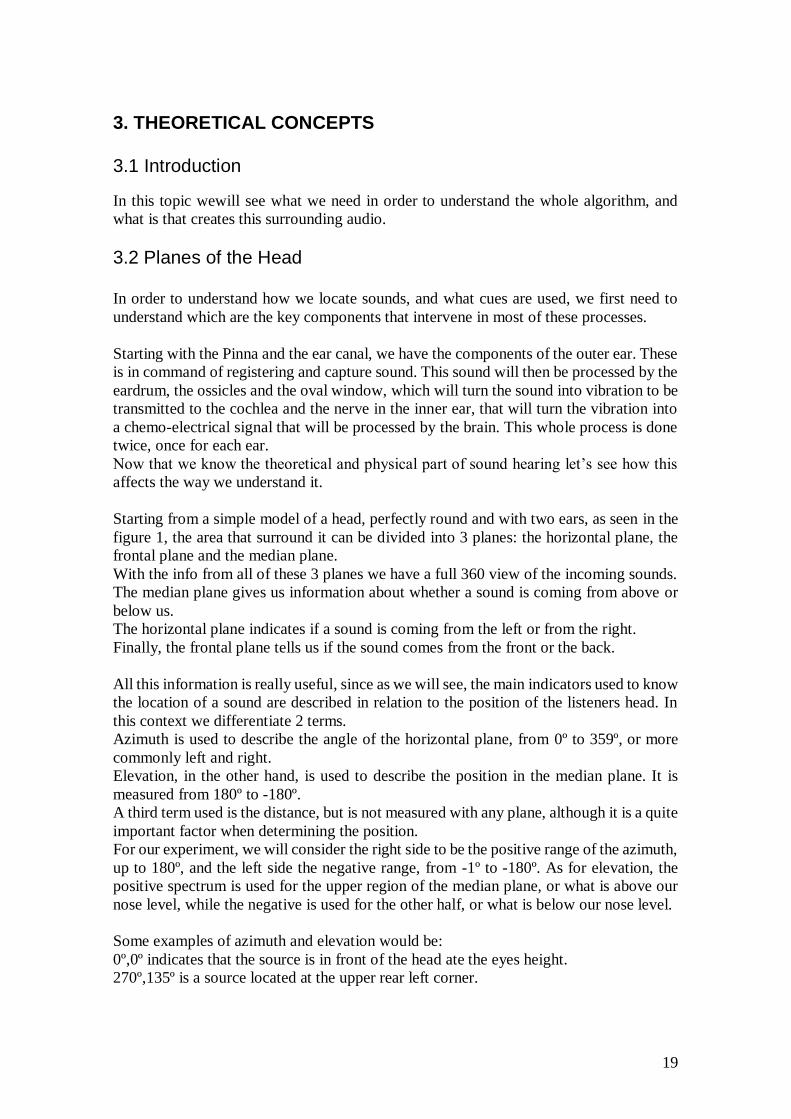
Starting from a simple model of a head, perfectly round and with two ears, as seen in the
figure 1, the area that surround it can be divided into 3 planes: the horizontal plane, the
frontal plane and the median plane.
With the info from all of these 3 planes we have a full 360 view of the incoming sounds.
The median plane gives us information about whether a sound is coming from above or
below us.
The horizontal plane indicates if a sound is coming from the left or from the right.
Finally, the frontal plane tells us if the sound comes from the front or the back.
All this information is really useful, since as we will see, the main indicators used to know
the location of a sound are described in relation to the position of the listeners head. In
this context we differentiate 2 terms.
Azimuth is used to describe the angle of the horizontal plane, from 0º to 359º, or more
commonly left and right.
Elevation, in the other hand, is used to describe the position in the median plane. It is
measured from 180º to -180º.
A third term used is the distance, but is not measured with any plane, although it is a quite
important factor when determining the position.
For our experiment, we will consider the right side to be the positive range of the azimuth,
up to 180º, and the left side the negative range, from -1º to -180º. As for elevation, the
positive spectrum is used for the upper region of the median plane, or what is above our
nose level, while the negative is used for the other half, or what is below our nose level.
Some examples of azimuth and elevation would be:
0º,0º indicates that the source is in front of the head ate the eyes height.
270º,135º is a source located at the upper rear left corner.
20
Figure 1. [6] Planes of the Head
The picture shows a representation of two of the planes, the Median and the Horizontal,
which are used to mesure the changes in the elevation and azimuth respectively. The
frontal plane missing in the picture is perperndicular to both of these.
3.3 Minimal Audible Angle Now that we know what is the factors that are used in sound location, we can detect a
stationary source. But what happens if the origin is moving?
In this case, we can still detect with a great degree of accuracy the location of the source.
This is known as the Minimal Audible Angle (MAA).
Of course, there are limitations for which the MAA will not give us a good result, but
within a given threshold we can safely discern it.
Some facts to take into account are the following:
• MAA is better, in terms of being more precise and having less variation at the front and
back positions (+- 3,6º and 5,5º) than at the laterals (+- 10º)
• MAA does not really work at the range of 1,5 to 2k Hz
• MAA is worse for vertical localization
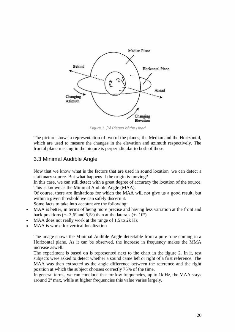
The image shows the Minimal Audible Angle detectable from a pure tone coming in a
Horizontal plane. As it can be observed, the increase in frequency makes the MMA
increase aswell.
The experiment is based on is represented next to the chart in the figure 2. In it, test
subjects were asked to detect whether a sound came left or right of a first reference. The
MAA was then extracted as the angle difference between the reference and the right
position at which the subject chooses correctly 75% of the time. In general terms, we can conclude that for low frequencies, up to 1k Hz, the MAA stays
around 2º max, while at higher frequencies this value varies largely.
21
Figure 2.[6] Minimal Audible Angle V Frequency
3.4 Interaural Time Difference Usually, when a sound is emitted, its waveform is seen as a circular wavefront when its
near, and as a plane wave when it is far away. The fact that our ears are located at each
side of the head is a byproduct of evolution, since sounds coming from around us are
easier to perceive than thous coming from below or above. In that field we are covered
by our ability to see and detect possible threats with our vision.
The Interaural Time Difference, or ITD, is the term that describes the time it takes
for a wave to arrive from its source to both ears, given that not always the source is
equidistant to both of them.
Let’s see an example:
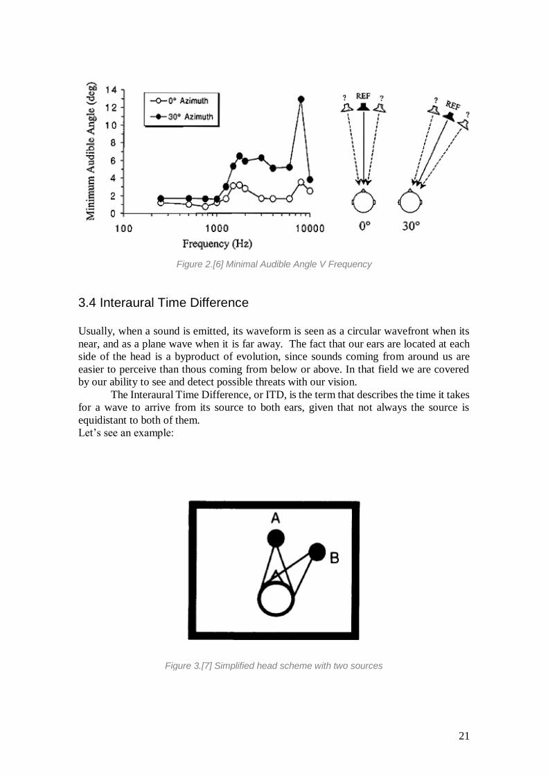
Figure 3.[7] Simplified head scheme with two sources
22
In the following picture we see a simplified round head with no ears, placed in the middle
of an anechoic chamber that provides no feedback to the audio. In this scenario two sound
sources appear. One located in front of the head, and one slightly tilted to the right side,
labeled A and B respectively.
In the first scenario, the source A emits a wave that, given that is located just in front of
the head, the distance to both ears is the same, so the sound will arrive at the same time
to both eardrums.
In the second scenario however, the source is tilted to the right, which means that the
distance to one of the ears is greater than the other. So, when the wavefront is emites, it
will arrive earlier to one of the eardrums. This delay between both ears when a sound is
emitted is known as Interaural Time Difference.
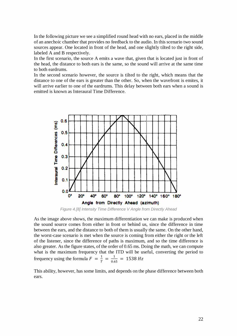
Figure 4.[8] Intensity Time Difference V Angle from Directly Ahead
As the image above shows, the maximum differentiation we can make is produced when
the sound source comes from either in front or behind us, since the difference in time
between the ears, and the distance to both of them is usually the same. On the other hand,
the worst-case scenario is met when the source is coming from either the right or the left
of the listener, since the difference of paths is maximum, and so the time difference is
also greater. As the figure states, of the order of 0.65 ms. Doing the math, we can compute
what is the maximum frequency that the ITD will be useful, converting the period to
frequency using the formula 𝐹 = 1
𝑇 =
1
0.65 = 1538 𝐻𝑧
This ability, however, has some limits, and depends on the phase difference between both
ears.
23
a) Limits of the ITD
As we have seen, if the time difference between the ears exceeds a certain value, we
cannot rely on it solely to determine the location of the sound.
Thus, we have the Interaural Phase Difference. This value is compressed between 0 and
2π. For very low frequencies, the IPD does not work well because of the similarity
between the signals in both ears, so we need to rely on the ITD.
As the phase difference increases it is easier to identify the sources, up until a certain
value that is.
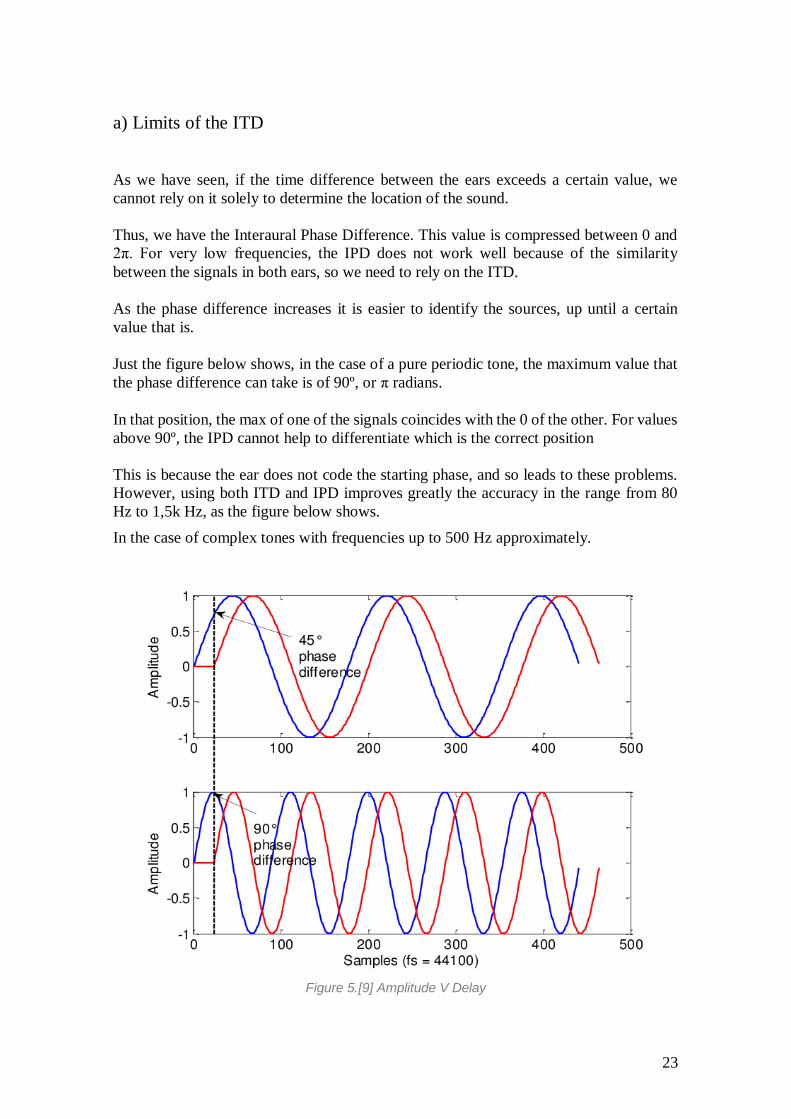
Just the figure below shows, in the case of a pure periodic tone, the maximum value that
the phase difference can take is of 90º, or π radians.
In that position, the max of one of the signals coincides with the 0 of the other. For values
above 90º, the IPD cannot help to differentiate which is the correct position
This is because the ear does not code the starting phase, and so leads to these problems.
However, using both ITD and IPD improves greatly the accuracy in the range from 80
Hz to 1,5k Hz, as the figure below shows.
In the case of complex tones with frequencies up to 500 Hz approximately.
Figure 5.[9] Amplitude V Delay
24
3.5 Interaural Intensity Difference
We have seen how the difference of paths between ears causes an effect we can profit to
locate sound sources, if the frequency is below 1,5k Hz. But what happens above that
value?
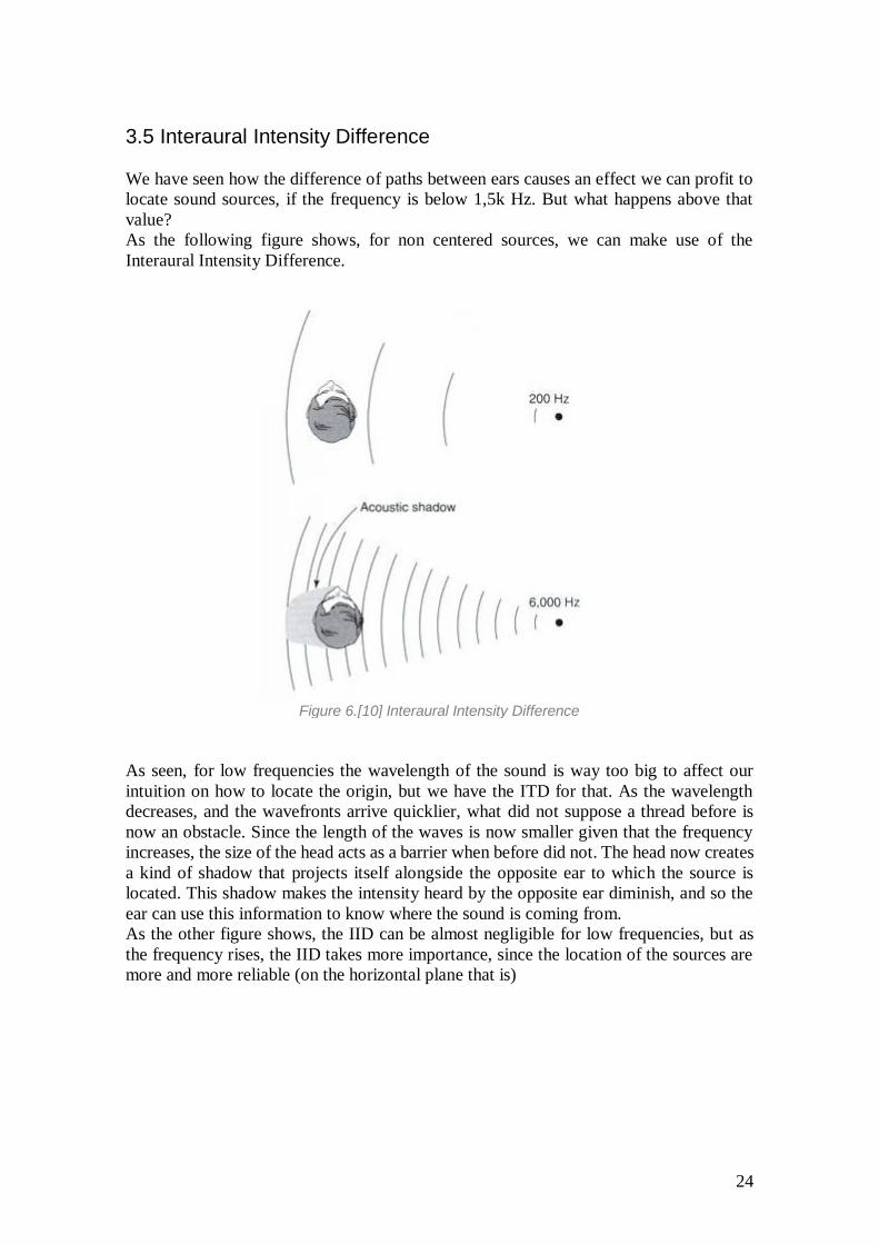
As the following figure shows, for non centered sources, we can make use of the
Interaural Intensity Difference.
Figure 6.[10] Interaural Intensity Difference
As seen, for low frequencies the wavelength of the sound is way too big to affect our
intuition on how to locate the origin, but we have the ITD for that. As the wavelength
decreases, and the wavefronts arrive quicklier, what did not suppose a thread before is
now an obstacle. Since the length of the waves is now smaller given that the frequency
increases, the size of the head acts as a barrier when before did not. The head now creates
a kind of shadow that projects itself alongside the opposite ear to which the source is
located. This shadow makes the intensity heard by the opposite ear diminish, and so the
ear can use this information to know where the sound is coming from.
As the other figure shows, the IID can be almost negligible for low frequencies, but as
the frequency rises, the IID takes more importance, since the location of the sources are
more and more reliable (on the horizontal plane that is)
25
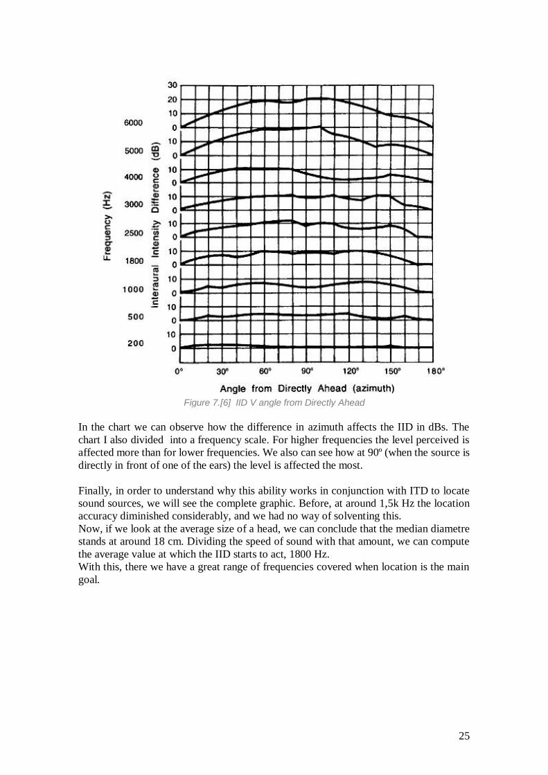
Figure 7.[6] IID V angle from Directly Ahead
In the chart we can observe how the difference in azimuth affects the IID in dBs. The
chart I also divided into a frequency scale. For higher frequencies the level perceived is
affected more than for lower frequencies. We also can see how at 90º (when the source is
directly in front of one of the ears) the level is affected the most.
Finally, in order to understand why this ability works in conjunction with ITD to locate
sound sources, we will see the complete graphic. Before, at around 1,5k Hz the location
accuracy diminished considerably, and we had no way of solventing this.
Now, if we look at the average size of a head, we can conclude that the median diametre
stands at around 18 cm. Dividing the speed of sound with that amount, we can compute
the average value at which the IID starts to act, 1800 Hz.
With this, there we have a great range of frequencies covered when location is the main
goal.
26
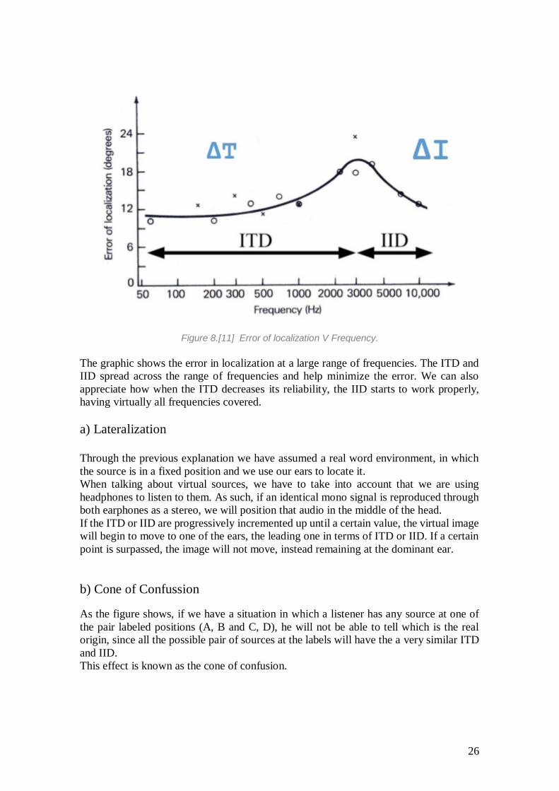
Figure 8.[11] Error of localization V Frequency.
The graphic shows the error in localization at a large range of frequencies. The ITD and
IID spread across the range of frequencies and help minimize the error. We can also
appreciate how when the ITD decreases its reliability, the IID starts to work properly,
having virtually all frequencies covered.
a) Lateralization
Through the previous explanation we have assumed a real word environment, in which
the source is in a fixed position and we use our ears to locate it.
When talking about virtual sources, we have to take into account that we are using
headphones to listen to them. As such, if an identical mono signal is reproduced through
both earphones as a stereo, we will position that audio in the middle of the head.
If the ITD or IID are progressively incremented up until a certain value, the virtual image
will begin to move to one of the ears, the leading one in terms of ITD or IID. If a certain
point is surpassed, the image will not move, instead remaining at the dominant ear.
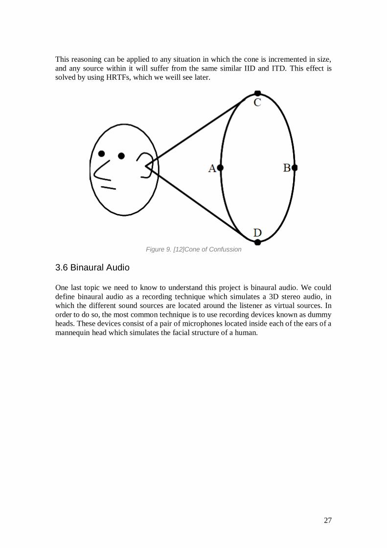
b) Cone of Confussion
As the figure shows, if we have a situation in which a listener has any source at one of
the pair labeled positions (A, B and C, D), he will not be able to tell which is the real
origin, since all the possible pair of sources at the labels will have the a very similar ITD
and IID.
This effect is known as the cone of confusion.
27
This reasoning can be applied to any situation in which the cone is incremented in size,
and any source within it will suffer from the same similar IID and ITD. This effect is
solved by using HRTFs, which we weill see later.
Figure 9. [12]Cone of Confussion
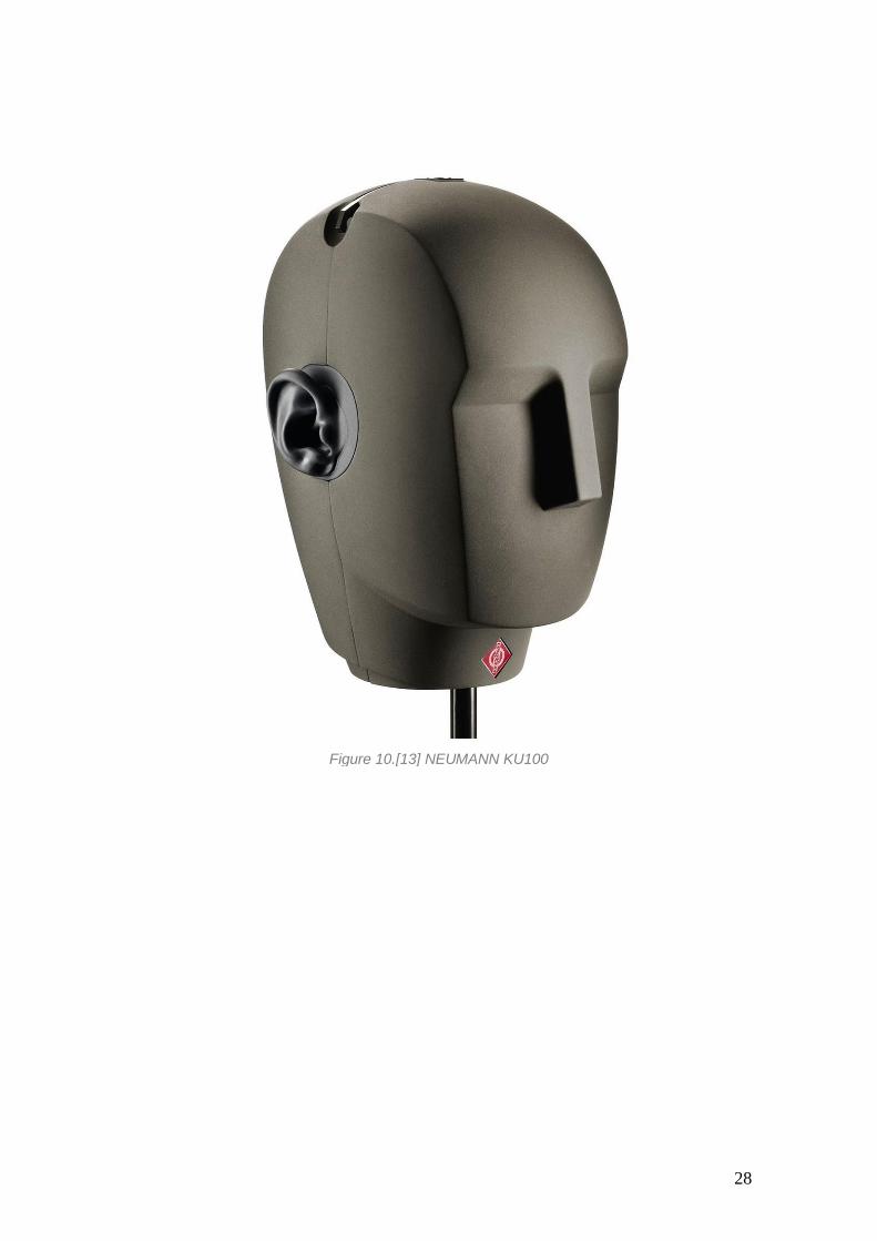
3.6 Binaural Audio One last topic we need to know to understand this project is binaural audio. We could
define binaural audio as a recording technique which simulates a 3D stereo audio, in
which the different sound sources are located around the listener as virtual sources. In
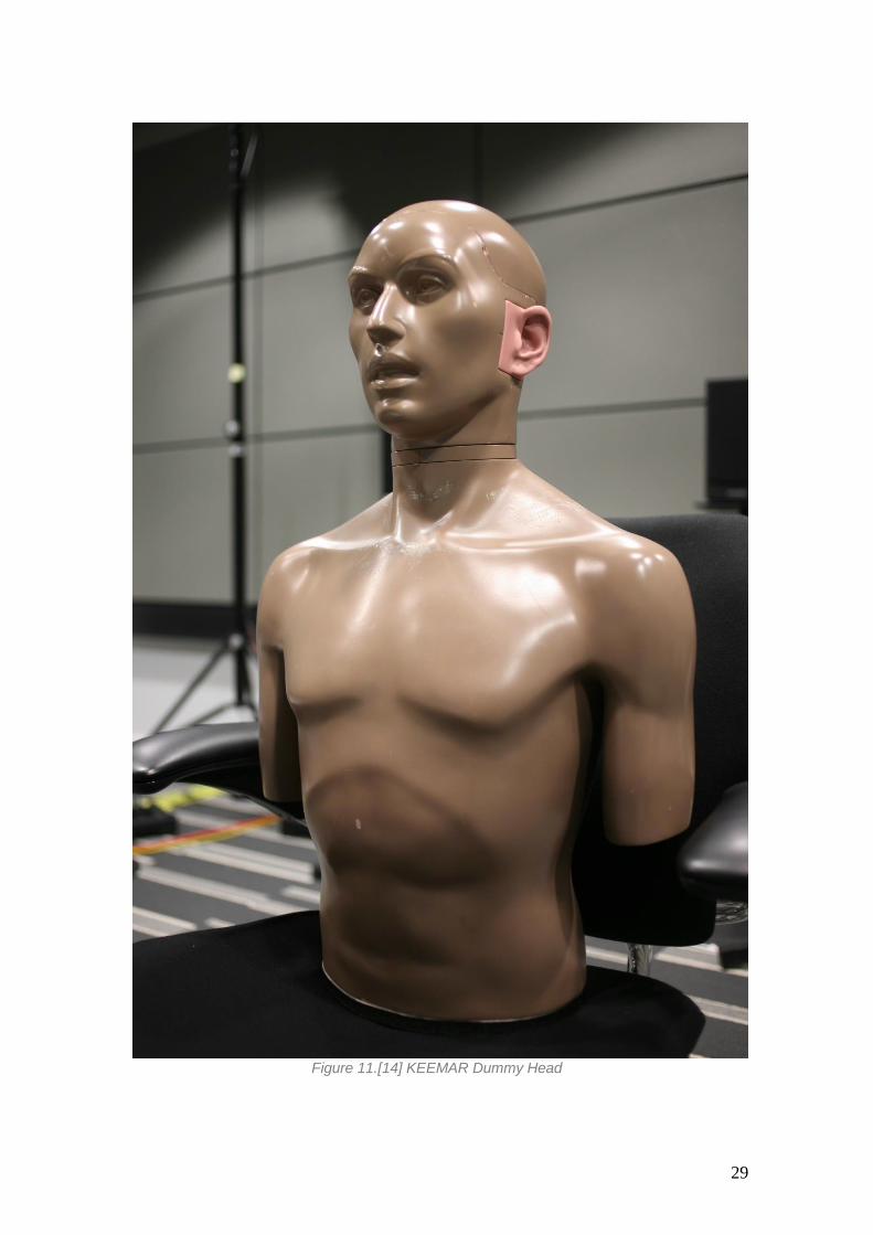
order to do so, the most common technique is to use recording devices known as dummy
heads. These devices consist of a pair of microphones located inside each of the ears of a
mannequin head which simulates the facial structure of a human.
28
Figure 10.[13] NEUMANN KU100
29
Figure 11.[14] KEEMAR Dummy Head
30
In order to understand how this relates to other more “common” types of recordings work,
let’s take a look at them.
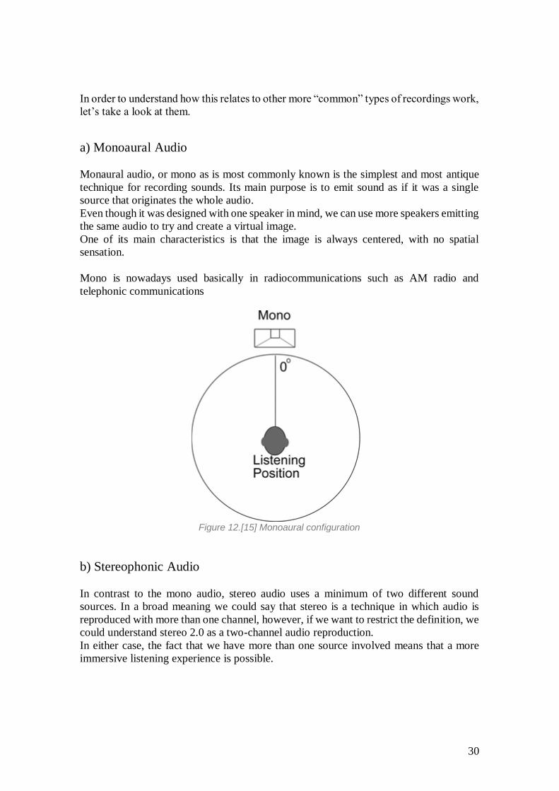
a) Monoaural Audio
Monaural audio, or mono as is most commonly known is the simplest and most antique
technique for recording sounds. Its main purpose is to emit sound as if it was a single
source that originates the whole audio.
Even though it was designed with one speaker in mind, we can use more speakers emitting
the same audio to try and create a virtual image.
One of its main characteristics is that the image is always centered, with no spatial
sensation.
Mono is nowadays used basically in radiocommunications such as AM radio and
telephonic communications
Figure 12.[15] Monoaural configuration
b) Stereophonic Audio
In contrast to the mono audio, stereo audio uses a minimum of two different sound
sources. In a broad meaning we could say that stereo is a technique in which audio is
reproduced with more than one channel, however, if we want to restrict the definition, we
could understand stereo 2.0 as a two-channel audio reproduction.
In either case, the fact that we have more than one source involved means that a more
immersive listening experience is possible.
31
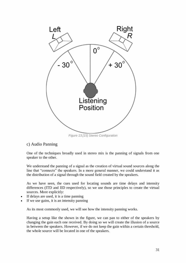
Figure 13.[15] Stereo Configuration
c) Audio Panning
One of the techniques broadly used in stereo mix is the panning of signals from one
speaker to the other.
We understand the panning of a signal as the creation of virtual sound sources along the
line that “connects” the speakers. In a more general manner, we could understand it as
the distribution of a signal through the sound field created by the speakers.
As we have seen, the cues used for locating sounds are time delays and intensity
differences (ITD and IID respectively), so we use those principles to create the virtual
sources. More explicitly:
• If delays are used, it is a time panning
• If we use gains, it is an intensity panning
As its most commonly used, we will see how the intensity panning works.
Having a setup like the shown in the figure, we can pan to either of the speakers by
changing the gain each one received. By doing so we will create the illusion of a source
in between the speakers. However, if we do not keep the gain within a certain threshold,
the whole source will be located in one of the speakers.
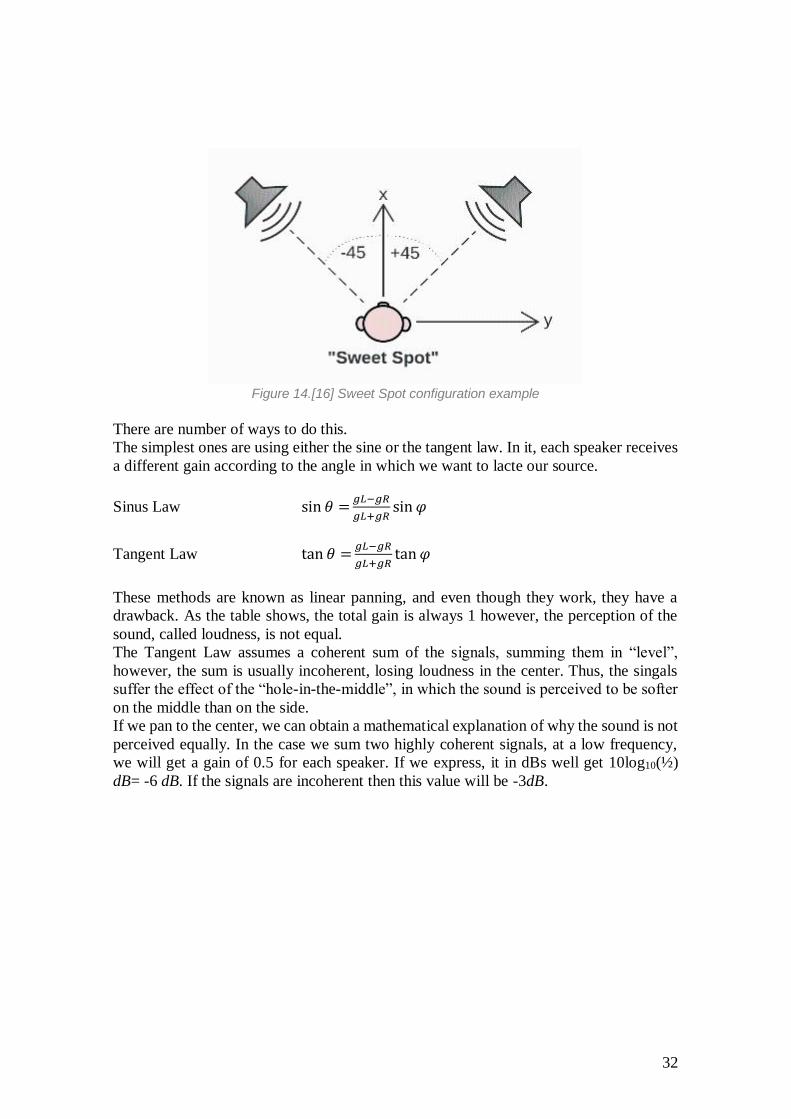
32
Figure 14.[16] Sweet Spot configuration example
There are number of ways to do this.
The simplest ones are using either the sine or the tangent law. In it, each speaker receives
a different gain according to the angle in which we want to lacte our source.
Sinus Law sin 𝜃 =𝑔𝐿−𝑔𝑅
𝑔𝐿+𝑔𝑅sin 𝜑
Tangent Law tan 𝜃 =𝑔𝐿−𝑔𝑅
𝑔𝐿+𝑔𝑅tan 𝜑
These methods are known as linear panning, and even though they work, they have a
drawback. As the table shows, the total gain is always 1 however, the perception of the
sound, called loudness, is not equal.
The Tangent Law assumes a coherent sum of the signals, summing them in “level”,
however, the sum is usually incoherent, losing loudness in the center. Thus, the singals
suffer the effect of the “hole-in-the-middle”, in which the sound is perceived to be softer
on the middle than on the side.
If we pan to the center, we can obtain a mathematical explanation of why the sound is not
perceived equally. In the case we sum two highly coherent signals, at a low frequency,
we will get a gain of 0.5 for each speaker. If we express, it in dBs well get 10log10(½)
dB= -6 dB. If the signals are incoherent then this value will be -3dB.
33
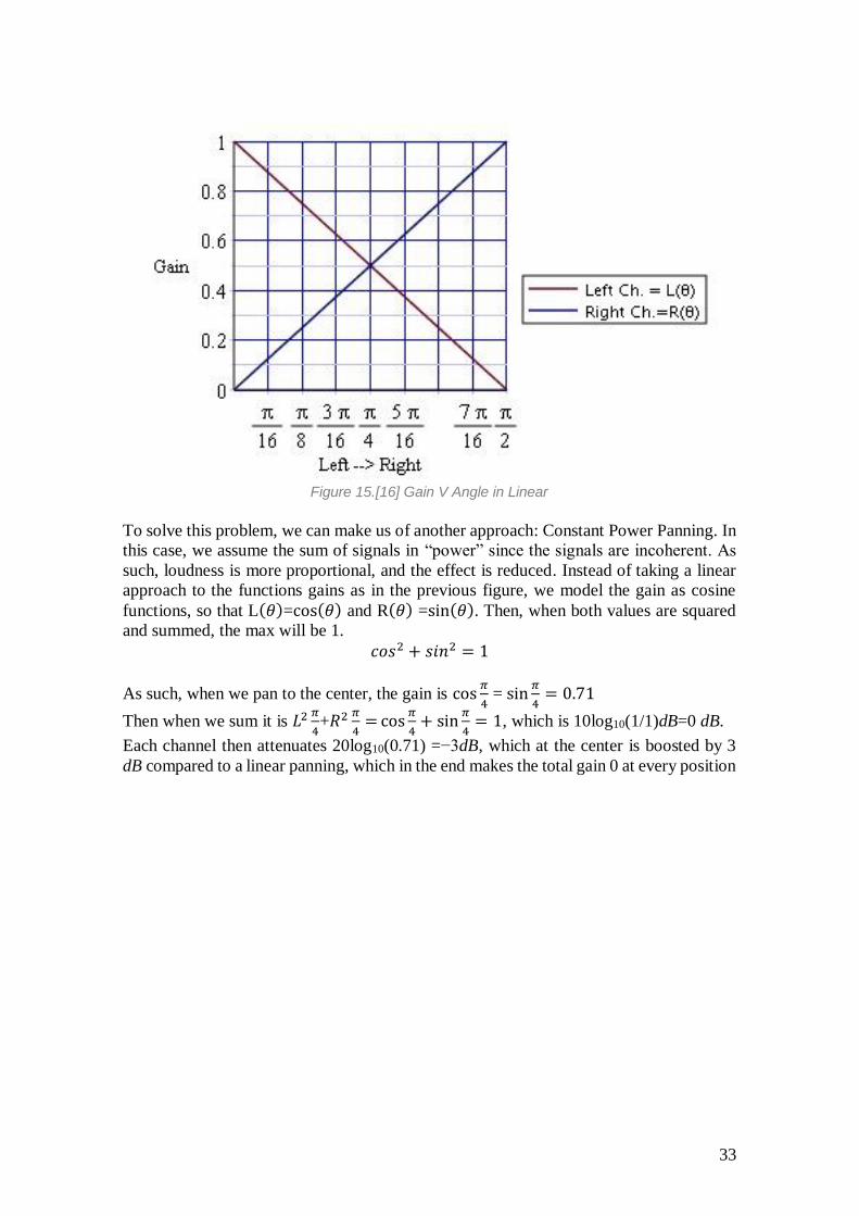
Figure 15.[16] Gain V Angle in Linear
To solve this problem, we can make us of another approach: Constant Power Panning. In
this case, we assume the sum of signals in “power” since the signals are incoherent. As
such, loudness is more proportional, and the effect is reduced. Instead of taking a linear
approach to the functions gains as in the previous figure, we model the gain as cosine
functions, so that L(𝜃)=cos(𝜃) and R(𝜃) =sin(𝜃). Then, when both values are squared
and summed, the max will be 1.
𝑐𝑜𝑠2 + 𝑠𝑖𝑛2 = 1
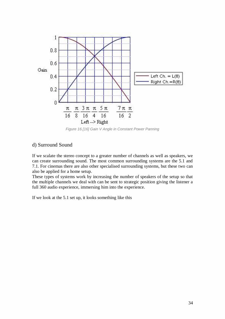
As such, when we pan to the center, the gain is cos𝜋
4 = sin
𝜋
4= 0.71
Then when we sum it is 𝐿2 𝜋
4+𝑅2 𝜋
4=cos
𝜋
4+ sin
𝜋
4= 1, which is 10log10(1/1)dB=0 dB.
Each channel then attenuates 20log10(0.71) =−3dB, which at the center is boosted by 3
dB compared to a linear panning, which in the end makes the total gain 0 at every position
34
Figure 16.[16] Gain V Angle in Constant Power Panning
d) Surround Sound
If we scalate the stereo concept to a greater number of channels as well as speakers, we
can create surrounding sound. The most common surrounding systems are the 5.1 and
7.1. For cinemas there are also other specialised surrounding systems, but these two can
also be applied for a home setup.
These types of systems work by increasing the number of speakers of the setup so that
the multiple channels we deal with can be sent to strategic position giving the listener a
full 360 audio experience, immersing him into the experience.
If we look at the 5.1 set up, it looks something like this
35
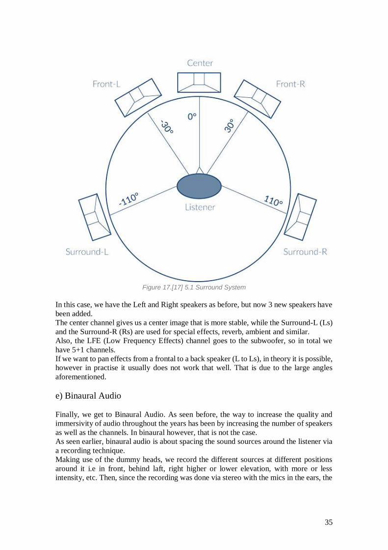
Figure 17.[17] 5.1 Surround System
In this case, we have the Left and Right speakers as before, but now 3 new speakers have
been added.
The center channel gives us a center image that is more stable, while the Surround-L (Ls)
and the Surround-R (Rs) are used for special effects, reverb, ambient and similar.
Also, the LFE (Low Frequency Effects) channel goes to the subwoofer, so in total we
have 5+1 channels.
If we want to pan effects from a frontal to a back speaker (L to Ls), in theory it is possible,
however in practise it usually does not work that well. That is due to the large angles
aforementioned.
e) Binaural Audio
Finally, we get to Binaural Audio. As seen before, the way to increase the quality and
immersivity of audio throughout the years has been by increasing the number of speakers
as well as the channels. In binaural however, that is not the case.
As seen earlier, binaural audio is about spacing the sound sources around the listener via
a recording technique.
Making use of the dummy heads, we record the different sources at different positions
around it i.e in front, behind laft, right higher or lower elevation, with more or less
intensity, etc. Then, since the recording was done via stereo with the mics in the ears, the
36
spatial information of the sources is on the recording, when listening to it, we can actually
locate the sources in their original position.
Still, there are other methods to record in binaural without using a dummy head.
• Synthetic Binaural
As stated, if we want to create a binaural audio without using the equipment mentioned,
we can synthesise a binaural file from a simple stereo. To do so we will need a pair of
HRTF (explained later). This ensures that the natural convolution that occurs during the
dummy head recording can be replicated with other files.
This method, while working, has a lower quality than the original as well as problems,
some of which are resoluble.
There is the problem of the back and front confusion, the externalization problem, in
which some sources are perceived inside the head, some localization errors and some
coloration issues in which the timbre is not right.
Since each person HRTFs is different, we can simply use personalized ones. Using head
tracking devices, we can solve the issue of not having head movements available. Adding
artificial reverberation, such as the room reverb or from a virtual space can work to solve
lack of reverb from the HRTFs (since usually they are recorded on anechoic rooms).
Via equalization tricks, the equalization effect from the mic or headphone can be resolved
and adding visual cues can work to deal with lack of them.
All of the above makes reference to the headphones experience, since binaural audio can
also work on a pair of speakers, receiving the name of transaural. However, we will not
cover that topic.
3.7 Head Related Transfer Function By now we should have a pretty clear understanding of how the auditory system works,
what cues we use to identify sound sources, and even what are some of the problems we
face both in real life and at a mathematical/physical level.
But how do we recreate a binaural sound from a stereo? We have seen how to create a
binaural sound using specialized equipment such as dummy heads, but in order to make
this project we do not have any of those tools. The answer is the Head Related Transfer
Function (HRTF).
Some of the factors that affect the way we hear are not dictated by our inner ears, but
from the shape of them, and its surrounding, like the torso, facial shape, hair and so. These
anatomical differences between humans makes us perceive sounds differently from one
another. In general terms mid to high frequencies get boosted, but the way each person
filters the sound varies, as the following figures shown.
37
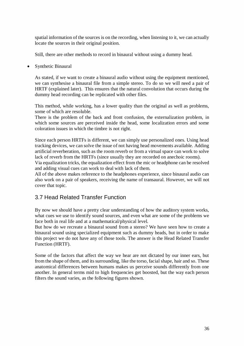
Figure 18.[7] HRTFs 135º azimuth
The chart shows the response of three people to the same stimulus, located at 135º and
45º azimuth. In this case we can see how the the main differences are located at the
highest frequencies.
38
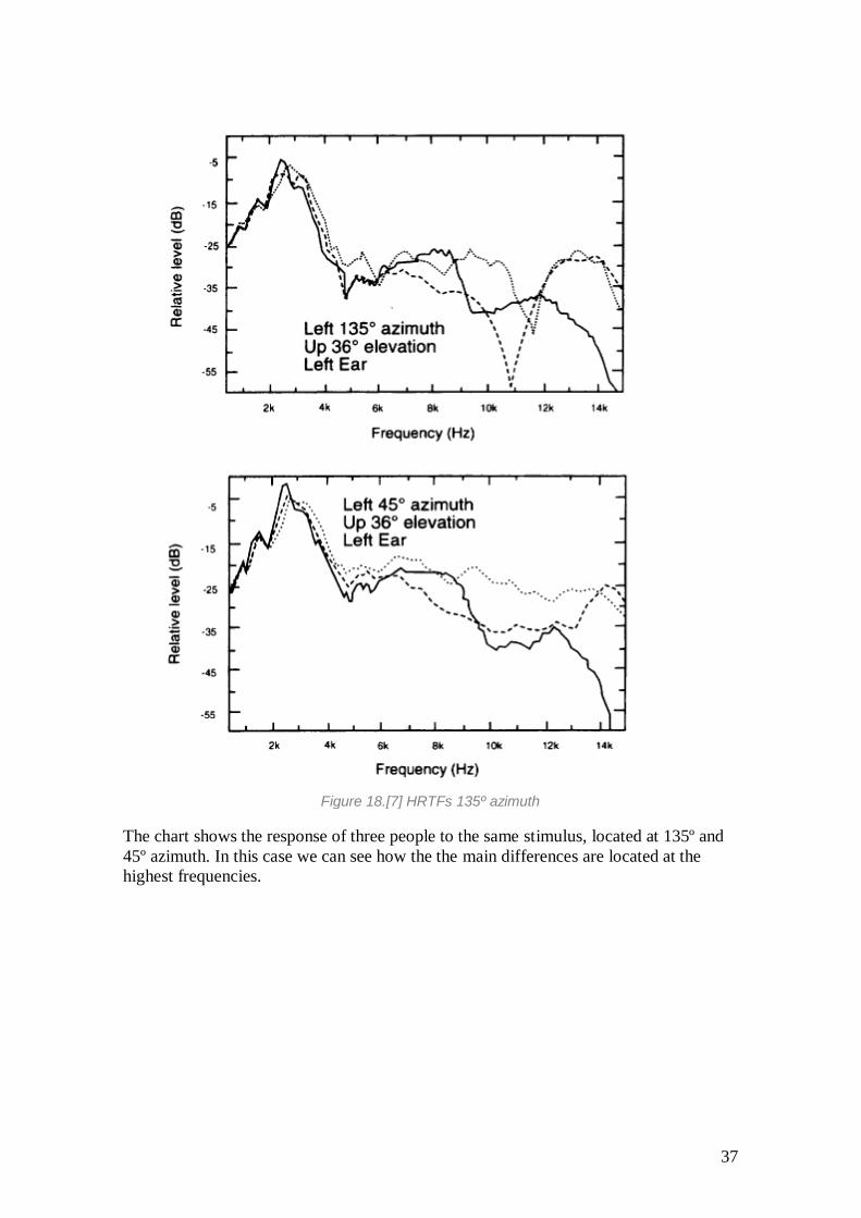
Figure 19.[7] HRTFs 90º azimuth
Just like in the previous case, we can observe the response of three people to the same
stimulus at different angles, and how their HRTFs are different. Again, most of the
differences are located at high frequencies.
39
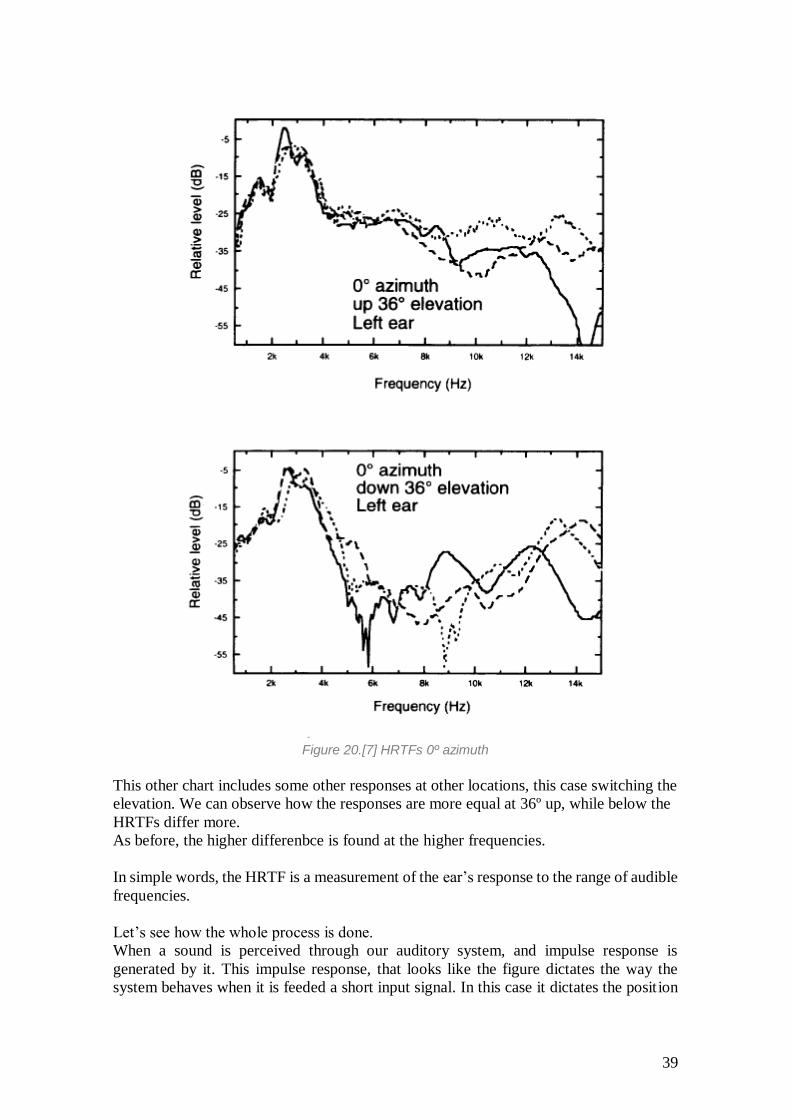
Figure 20.[7] HRTFs 0º azimuth
This other chart includes some other responses at other locations, this case switching the
elevation. We can observe how the responses are more equal at 36º up, while below the
HRTFs differ more.
As before, the higher differenbce is found at the higher frequencies.
In simple words, the HRTF is a measurement of the ear’s response to the range of audible
frequencies.
Let’s see how the whole process is done.
When a sound is perceived through our auditory system, and impulse response is
generated by it. This impulse response, that looks like the figure dictates the way the
system behaves when it is feeded a short input signal. In this case it dictates the posit ion
40
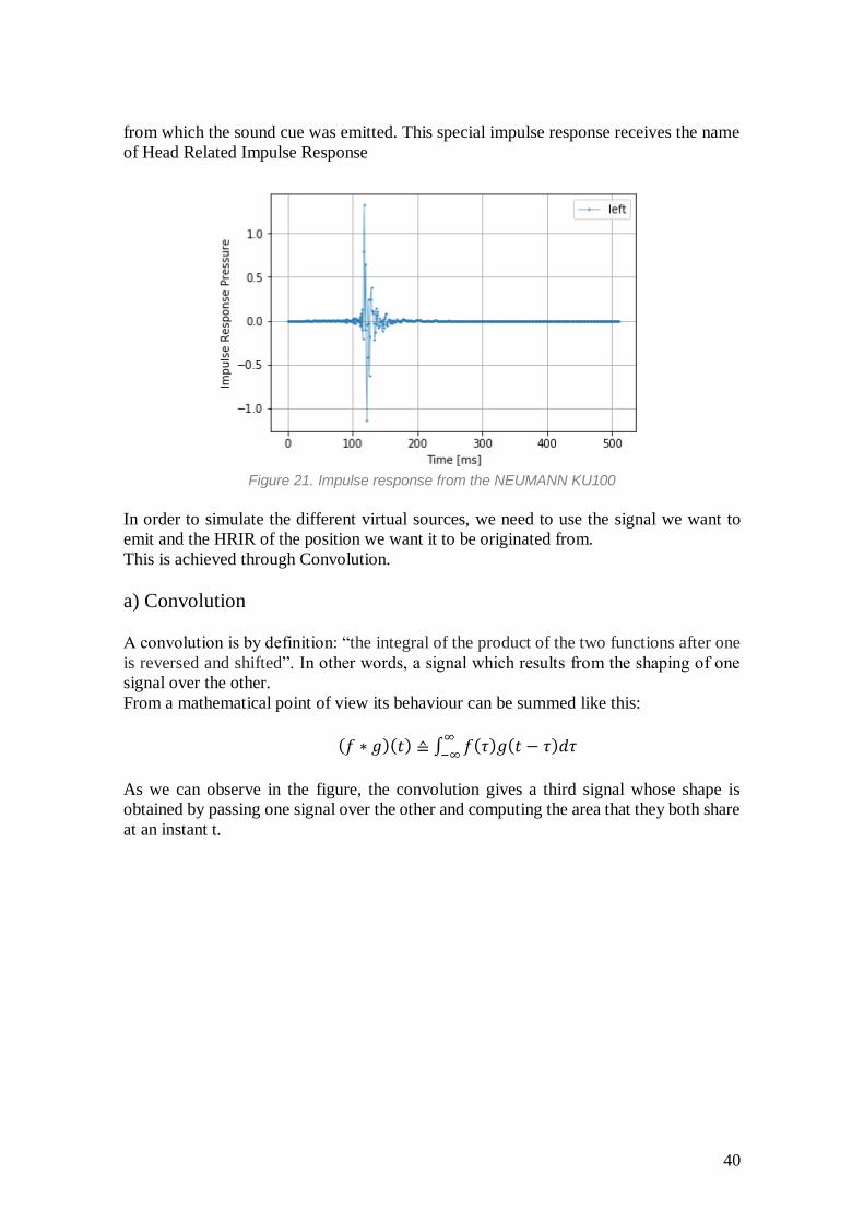
from which the sound cue was emitted. This special impulse response receives the name
of Head Related Impulse Response
Figure 21. Impulse response from the NEUMANN KU100
In order to simulate the different virtual sources, we need to use the signal we want to
emit and the HRIR of the position we want it to be originated from.
This is achieved through Convolution.
a) Convolution
A convolution is by definition: “the integral of the product of the two functions after one
is reversed and shifted”. In other words, a signal which results from the shaping of one
signal over the other.
From a mathematical point of view its behaviour can be summed like this:
(𝑓 ∗ 𝑔)(𝑡) ≙ ∫ 𝑓(𝜏)𝑔(𝑡 − 𝜏)𝑑𝜏∞
−∞
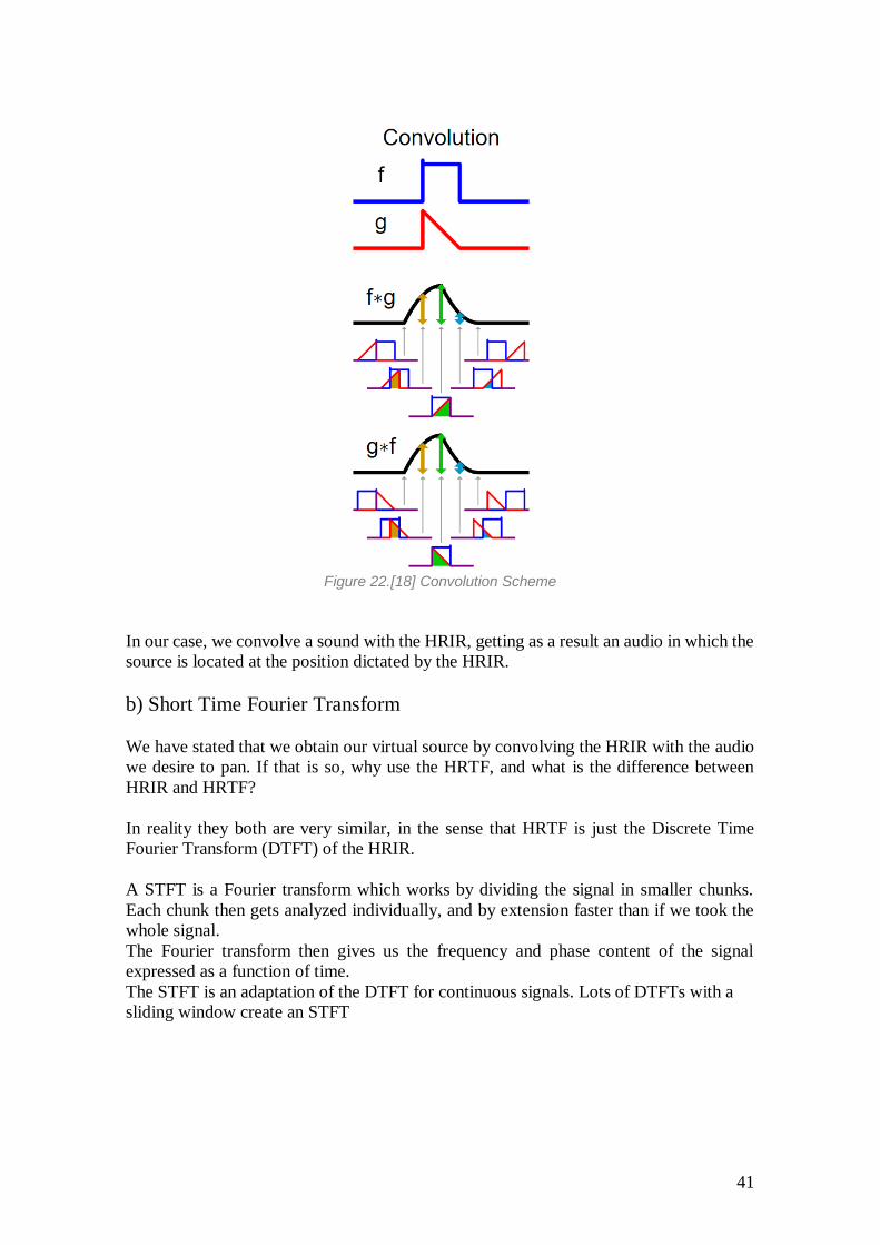
As we can observe in the figure, the convolution gives a third signal whose shape is
obtained by passing one signal over the other and computing the area that they both share
at an instant t.
41
Figure 22.[18] Convolution Scheme
In our case, we convolve a sound with the HRIR, getting as a result an audio in which the
source is located at the position dictated by the HRIR.
b) Short Time Fourier Transform
We have stated that we obtain our virtual source by convolving the HRIR with the audio
we desire to pan. If that is so, why use the HRTF, and what is the difference between
HRIR and HRTF?
In reality they both are very similar, in the sense that HRTF is just the Discrete Time
Fourier Transform (DTFT) of the HRIR.
A STFT is a Fourier transform which works by dividing the signal in smaller chunks.
Each chunk then gets analyzed individually, and by extension faster than if we took the
whole signal.
The Fourier transform then gives us the frequency and phase content of the signal
expressed as a function of time.
The STFT is an adaptation of the DTFT for continuous signals. Lots of DTFTs with a
sliding window create an STFT
42
c) Cross-Correlation
In more or less the same fashion as the Convolution, the cross-correlation and the
autocorrelation share a common mathematical basis. If the convolution is the result of
shaping a signal using another, the cross-correlation is the movement of one relative to
the other.
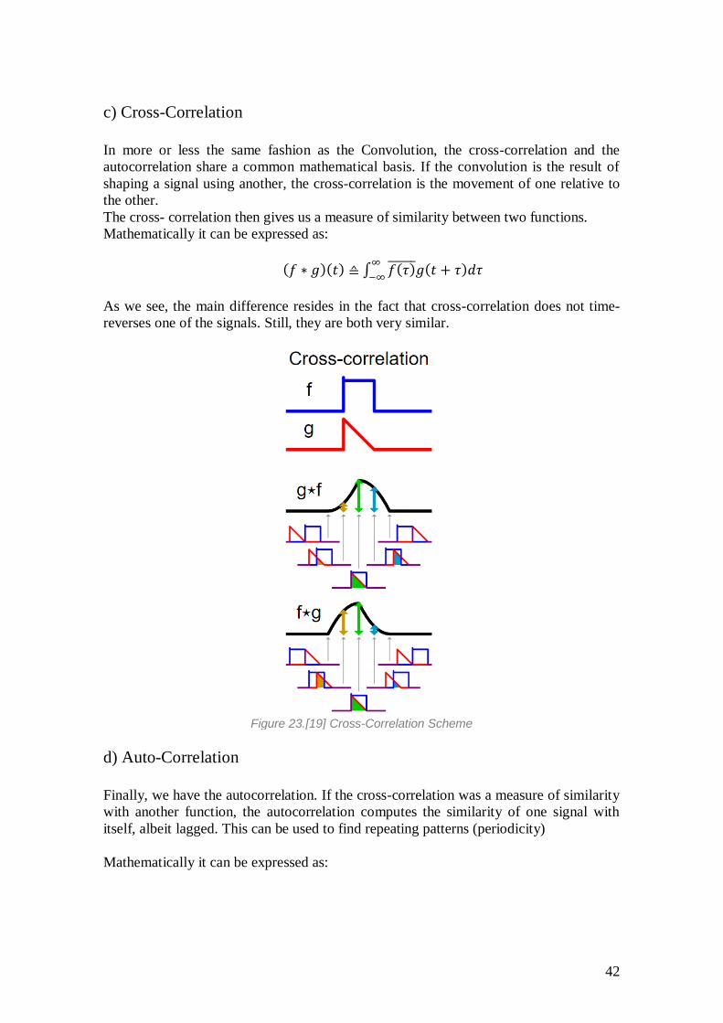
The cross- correlation then gives us a measure of similarity between two functions.
Mathematically it can be expressed as:
(𝑓 ∗ 𝑔)(𝑡) ≙ ∫ 𝑓(𝜏) 𝑔(𝑡 + 𝜏)𝑑𝜏∞
−∞
As we see, the main difference resides in the fact that cross-correlation does not time-
reverses one of the signals. Still, they are both very similar.
Figure 23.[19] Cross-Correlation Scheme
d) Auto-Correlation
Finally, we have the autocorrelation. If the cross-correlation was a measure of similarity
with another function, the autocorrelation computes the similarity of one signal with
itself, albeit lagged. This can be used to find repeating patterns (periodicity)
Mathematically it can be expressed as:
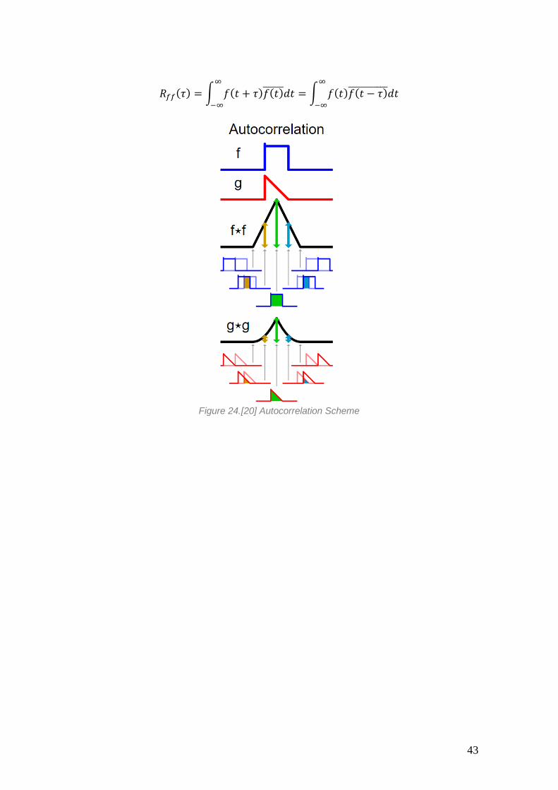
43
𝑅𝑓𝑓(𝜏) = ∫ 𝑓(𝑡 + 𝜏)𝑓(𝑡) 𝑑𝑡∞
−∞
= ∫ 𝑓(𝑡)𝑓(𝑡 − 𝜏) 𝑑𝑡∞
−∞
Figure 24.[20] Autocorrelation Scheme

44
45
4. PROPOSED SOLUTION
4.1 Paper we based our work on Now that we have the full knowledge to correctly understand the problem and the
solution, let’s see what our starting point is.
As stated, our goal is to make an implementation of two methods described in the paper
by Merimaa, Goodwin and Jot to extract the Ambience and Direct components of a mix,
and from there, create a synthetic binaural stereo file making use of a database of HRIRs.
In this binaural file, the different components extracted using the methods are used to
establish the spatial components and create a sense of surrounding by the sources.
Let’s go step by step alongside the paper.
First of all, we need to define the way in which we are going to work. In this case, the
whole method is designed to be performed in frequency-domain signals, so the first thing
we will need to do is to convert the samples of the audio file using the Short Time Fourier
Transform (STFT) to be in said domain.
As some of the functions used have multiple instances of dividing between coefficients,
we want to avoid having in one of the cases a NaN (Not a Number) result (usually this
happens when we try to divide a number by 0). To avoid this, before doing the STFT, we
add to the whole file a small value of random gaussian noise, with mean of 1^-100 and
standard deviation of 1^-50. Doing this prevents the NaN problem and is unnoticeable in
the final audio file.
As stated by the paper: “Many of the results derived in this paper are expressed
in terms of correlations of the two input signals.” As such, we will have to compute the
Auto and Cross-Correlation content of both channels (Left and Right)
(1,2,3)
𝑟𝐿𝐿 = 𝑋𝐿𝐻 𝑋𝐿 = ∑𝑥𝐿[𝑖]
∗
𝑁
𝑖=1
𝑥𝐿[𝑖] = ||𝑋𝐿 ||2
rRR = XRH XR = ∑xR[i]∗
N
i=1
xR[i] = ||XR ||2
rLR = XLH XR = ∑xL[i]
∗
N
i=1
xR[i] = rRL∗
In the formulas above, Rll is the autocorrelation of the left channel, Rrr the autocorrelation
of the right channel, and Rlr the cross-correlation of both channels.
However, these formulas do not apply for a real time implementation, being only the
theoretical approach to the concepts.
To correctly achieve the cross and autocorrelations of both channels, we will have to look
at the point 5 of the paper, in which the following formulas can be extracted.
(34)
46
rLL(t) = λrLL(t − 1) + (1 − λ)XL∗(t)XL(t)
rRR(t) = λrRR(t − 1) + (1 − λ)XR∗ (t)XR(t)
rLR(t) = λrLR(t − 1) + (1 − λ)XL∗ (t)XR(t)
(35)
τ = −1
fcln(1 − λ)
Just as the paper states, these formulas are approximated via recursivity, and making use
of a forgetting factor lambda between 0 and 1. This lambda will dictate how many of the
previous samples we take to compute the following iteration.
Starting at t = 0, we only have the current value of the auto and crosscorrelation multiplied
by a factor 1-lambda. If lambda is 0.5, we will only take half the value.
At t=1, we have the actual plus the previous one, both of them multiplied by a factor. At
this time however, we will have 0.5*0.5 of the previous and 0.5 of the actual. At t=2,
0.5*0.5*0.5 of the first 0.5*0.5 of the second and 0.5 of the actual, and so on.
This forgetting factor can be approximated utilizing the previous formula, but doing tests,
we have found that 0.7 is a value that gives great results.
Also, we have the cross-correlation coefficient which will be used quite often in the
computations, and is defined as the following equation
(4)
ϕLR =rLR
√rLLrRR=
XLH XR
||XL || ||XR
||
Finally, we will use a very simple approach to the signal model, in which the signal is
composed by two factors: a single primary component and ambience. Among other
assumptions, this means that the primary signals are identical but for the phase and level
differences.
(5)
XL = PL
+ AL
XR = PR
+ AR
(6)
||XL ||2 = ||PL
||2 + ||AL ||2
||XR ||2 = ||PR
||2 + ||AR ||2
(7)
rLR = PLH PR
(8)
||rLR|| = ||PL || ||PR ||
In order to obtain both of these components, we will work with masks. These said masks
are in fact matrixes of values that range from 0 to 1 with all the possibilities in between.
Multiplying our matrix of values from the file in the time-frequency domain by the mask
allows us to let some of these values go through and some not. This subsequently
separates the file in the two components: ambience and primary. The following equation
shows the ambience signals left and right (𝐴L and 𝐴𝑅 )
47
(9) 𝐴L(t, f) = αL(t, f)XL(t, f)
𝐴𝑅(𝑡, 𝑓) = 𝛼𝑅(𝑡, 𝑓)𝑋𝑅(𝑡, 𝑓)
These extraction masks, should correspond to the amount of ambience of each channel,
as the following equation indicates
(10)
αL =||AL ||
||XL ||
, 𝛼𝑅 =||𝐴𝑅 ||
||𝑋𝑅 ||
Having the basis for our algorithms, let’s now take a look at them.
The first one assumes that the ratio of ambience in both channels is equal, so
αL 𝑎𝑛𝑑 αR 𝑎𝑟𝑒 𝑒𝑞𝑢𝑎𝑙. As explained, in previous work by the authors of the paper, a binary
mask was used to separate ambience from primary which did not work most of the time,
so a soft decision was introduced to make the mask work better. This led to a nonlinear
function.
(11) αcom = Γ(1 − |ϕLR |)
Still, there is another option, which is to force the ambience masks of both channels to be
equal, and solving the system formed by equations 6,8 and 10. In doing so, the value for
the mask is defined as the following equation shows:
(12)
αcom = √1 − |ϕLR |
Which satisfies the nonlinearity function requirement. Regarding the common mask, as
we assumed that the ratio of ambience is equal, means that if the audio we use does not
fulfil this condition we will have problems. As the following equation shows, if one of
the channels is to be empty, the mask will not be correctly computed.
(13)
||AL ||
||XL ||
=||AR ||
||XR ||
= αcom
The second method justifies his supposition on the fact that the level of ambience in a
stereo recording is usually the same in both channels, and so it is logical to conclude that
(14)
||AL || = ||AR
|| = IA
Following this basis, and resolving the system formed by the equations 6,8 and 14, the
cross-correlation value can be computed as
(15) ||rLR||2 = IA
4 − IA2(rLL + rRR) + rLL
2 rRR2
Since we want the value of the ambience, i.e Ia, we can use the following function
provided by the paper.
(16)
IA2 =
1
2(rLL + rRR − √(rLL − rRR)2 + 4||rLR||2)
48
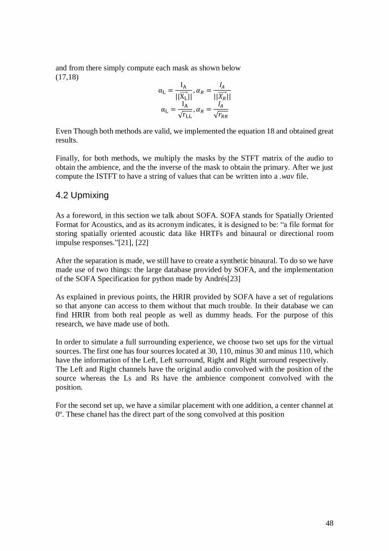
and from there simply compute each mask as shown below
(17,18)
αL =IA
||XL ||
, 𝛼𝑅 =𝐼𝐴
||𝑋𝑅 ||
αL =IA
√rLL, 𝛼𝑅 =
𝐼𝐴
√𝑟𝑅𝑅
Even Though both methods are valid, we implemented the equation 18 and obtained great
results.
Finally, for both methods, we multiply the masks by the STFT matrix of the audio to
obtain the ambience, and the the inverse of the mask to obtain the primary. After we just
compute the ISTFT to have a string of values that can be written into a .wav file.
4.2 Upmixing As a foreword, in this section we talk about SOFA. SOFA stands for Spatially Oriented
Format for Acoustics, and as its acronym indicates, it is designed to be: “a file format for
storing spatially oriented acoustic data like HRTFs and binaural or directional room
impulse responses.”[21], [22]
After the separation is made, we still have to create a synthetic binaural. To do so we have
made use of two things: the large database provided by SOFA, and the implementation
of the SOFA Specification for python made by Andrés[23]
As explained in previous points, the HRIR provided by SOFA have a set of regulations
so that anyone can access to them without that much trouble. In their database we can
find HRIR from both real people as well as dummy heads. For the purpose of this
research, we have made use of both.
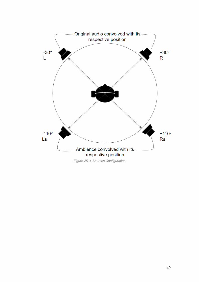
In order to simulate a full surrounding experience, we choose two set ups for the virtual
sources. The first one has four sources located at 30, 110, minus 30 and minus 110, which
have the information of the Left, Left surround, Right and Right surround respectively.
The Left and Right channels have the original audio convolved with the position of the
source whereas the Ls and Rs have the ambience component convolved with the
position.
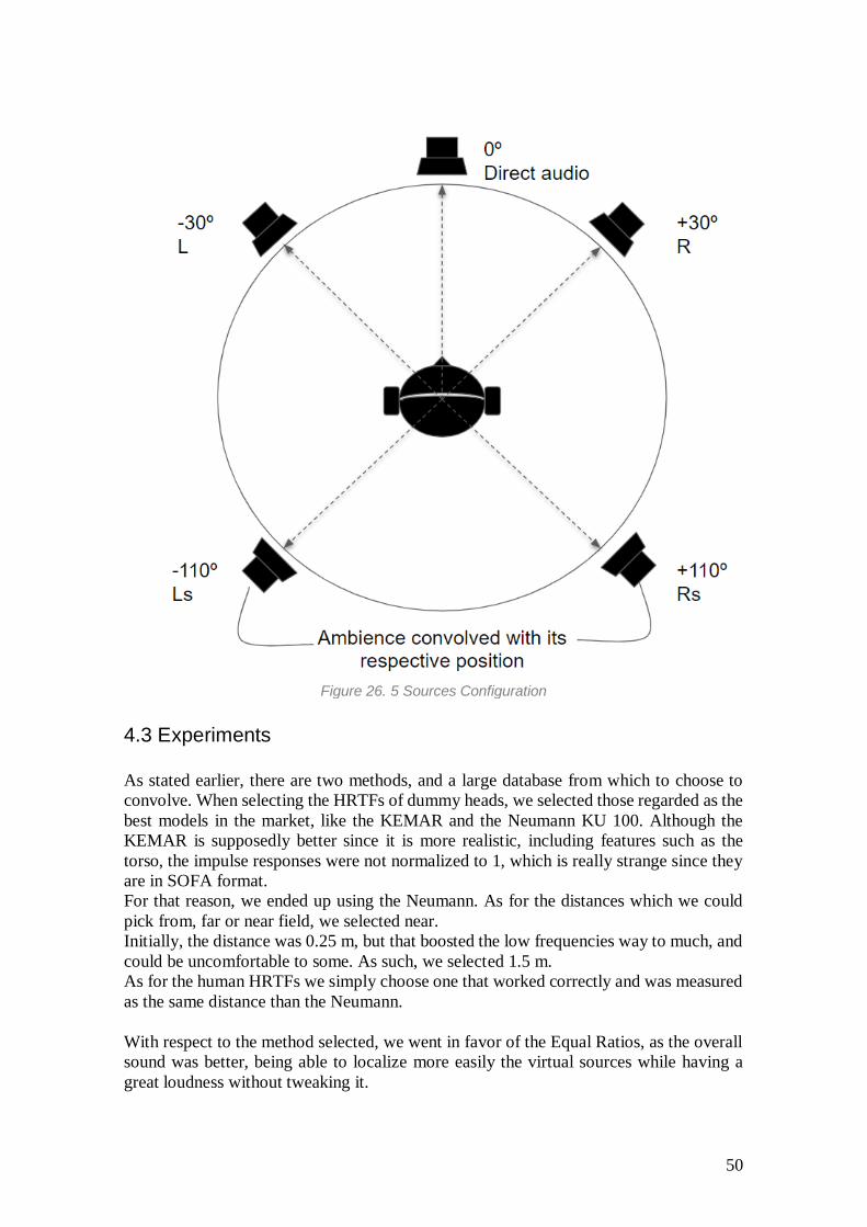
For the second set up, we have a similar placement with one addition, a center channel at
0º. These chanel has the direct part of the song convolved at this position
49
Figure 25. 4 Sources Configuration
50
Figure 26. 5 Sources Configuration
4.3 Experiments As stated earlier, there are two methods, and a large database from which to choose to
convolve. When selecting the HRTFs of dummy heads, we selected those regarded as the
best models in the market, like the KEMAR and the Neumann KU 100. Although the
KEMAR is supposedly better since it is more realistic, including features such as the
torso, the impulse responses were not normalized to 1, which is really strange since they
are in SOFA format.
For that reason, we ended up using the Neumann. As for the distances which we could
pick from, far or near field, we selected near.
Initially, the distance was 0.25 m, but that boosted the low frequencies way to much, and
could be uncomfortable to some. As such, we selected 1.5 m.
As for the human HRTFs we simply choose one that worked correctly and was measured
as the same distance than the Neumann.
With respect to the method selected, we went in favor of the Equal Ratios, as the overall
sound was better, being able to localize more easily the virtual sources while having a
great loudness without tweaking it.
51
Regarding the environment, we choose python since there are a great deal of libraries
which are dedicated to audio, and so is really easy find already done implementations of
essential things, such as reading and writing audios, Fourier Transforms and so. Besides,
it is a programming language used commonly, so getting some practise and experience is
always great.
As for the performance of the algorithm, we would argue that is pretty correct. For audios
of 40 seconds, the algorithm takes no more than 60 seconds to separate Ambience and
Primary, while the upmixing is almost instantaneous.
Finally, the whole code with both implementations, examples, and unused methods is
online abialable for free at GitHub[24] so that anyone can try it out.

52
53
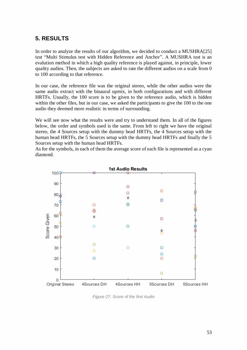
5. RESULTS In order to analyze the results of our algorithm, we decided to conduct a MUSHRA[25]
test “Multi Stimulus test with Hidden Reference and Anchor”. A MUSHRA test is an
evalution method in which a high quality reference is played against, in principle, lower
quality audios. Then, the subjects are asked to rate the different audios on a scale from 0
to 100 according to that reference.
In our case, the reference file was the original stereo, while the other audios were the
same audio extract with the binaural upmix, in both configurations and with different
HRTFs. Usually, the 100 score is to be given to the reference audio, which is hidden
within the other files, but in our case, we asked the participants to give the 100 to the one
audio they deemed more realistic in terms of surrounding.
We will see now what the results were and try to understand them. In all of the figures
below, the order and symbols used is the same. From left to right we have the original
stereo, the 4 Sources setup with the dummy head HRTFs, the 4 Sources setup with the
human head HRTFs, the 5 Sources setup with the dummy head HRTFs and finally the 5
Sources setup with the human head HRTFs.
As for the symbols, in each of them the average score of each file is represented as a cyan
diamond.
Figure 27. Score of the first Audio
54
In this first figure we can observe that altough there are a couple that stand out as average
scores, the difference throughout is not that astonishing.
Generally, we can observe how the 5 sources configuration seems to be worse overall.
This may be because in a crowded sound space as the one from the first file, the extra
sorce blurs the differents sources into one large body in the center.
This first file corresponds to the song Jambú[26], which is compossed of a variety of
instruments such as a saxo, trumpet, trombone, bass, electric guitar, battery and some sets
of drums. This mix creates a whole volume which is really powerfull by itself. If the
combination or location of the fonts is not correctly choosen, or the gains are not quite on
point, the quality of the listening really decays.
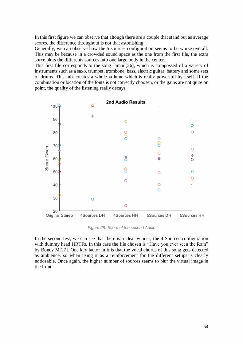
Figure 28. Score of the second Audio
In the second test, we can see that there is a clear winner, the 4 Sources configuration
with dummy head HRTFs. In this case the file chosen is “Have you ever seen the Rain”
by Boney M[27]. One key factor in it is that the vocal chorus of this song gets detected
as ambience, so when using it as a reinforcement for the different setups is clearly
noticeable. Once again, the higher number of sources seems to blur the virtual image in
the front.
55
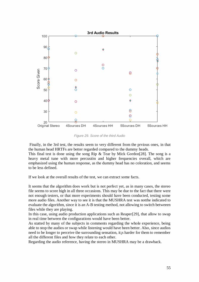
Figure 29. Score of the third Audio
Finally, in the 3rd test, the results seem to very different from the prvious ones, in that
the human head HRTFs are better regarded compared to the dummy heads.
This final test is done using the song Rip & Tear by Mick Gordon[28]. The song is a
heavy metal tune with more percusión and higher frequencies overall, which are
emphasized using the human response, as the dummy head has no coloration, and seems
to be less defined.
If we look at the overall results of the test, we can extract some facts.
It seems that the algorithm does work but is not perfect yet, as in many cases, the stereo
file seems to score high in all three occasions. This may be due to the fact that there were
not enough testers, or that more experiments should have been conducted, testing some
more audio files. Another way to see it is that the MUSHRA test was notthe indicated to
evaluate the algorithm, since it is an A-B testing method, not allowing to switch betweeen
files while they are playing.
In this case, using audio production applications such as Reaper[29], that allow to swap
in real time between the configurations would have been better.
As statted by many of the subjects in comments regarding the whole experience, being
able to stop the audios or swap while listening would have been better. Also, since audios
need to be longer to perceive the surrounding sensation, it¡s harder for them to remember
all the different files and how they relate to each other.
Regarding the audio reference, having the stereo in MUSHRA may be a drawback.
56
In MUSHRA the reference always plays within the other configurations as another rfile,
while in Reaper, swapping between it and the others accentuates the differences and
changes made by the algorithm.
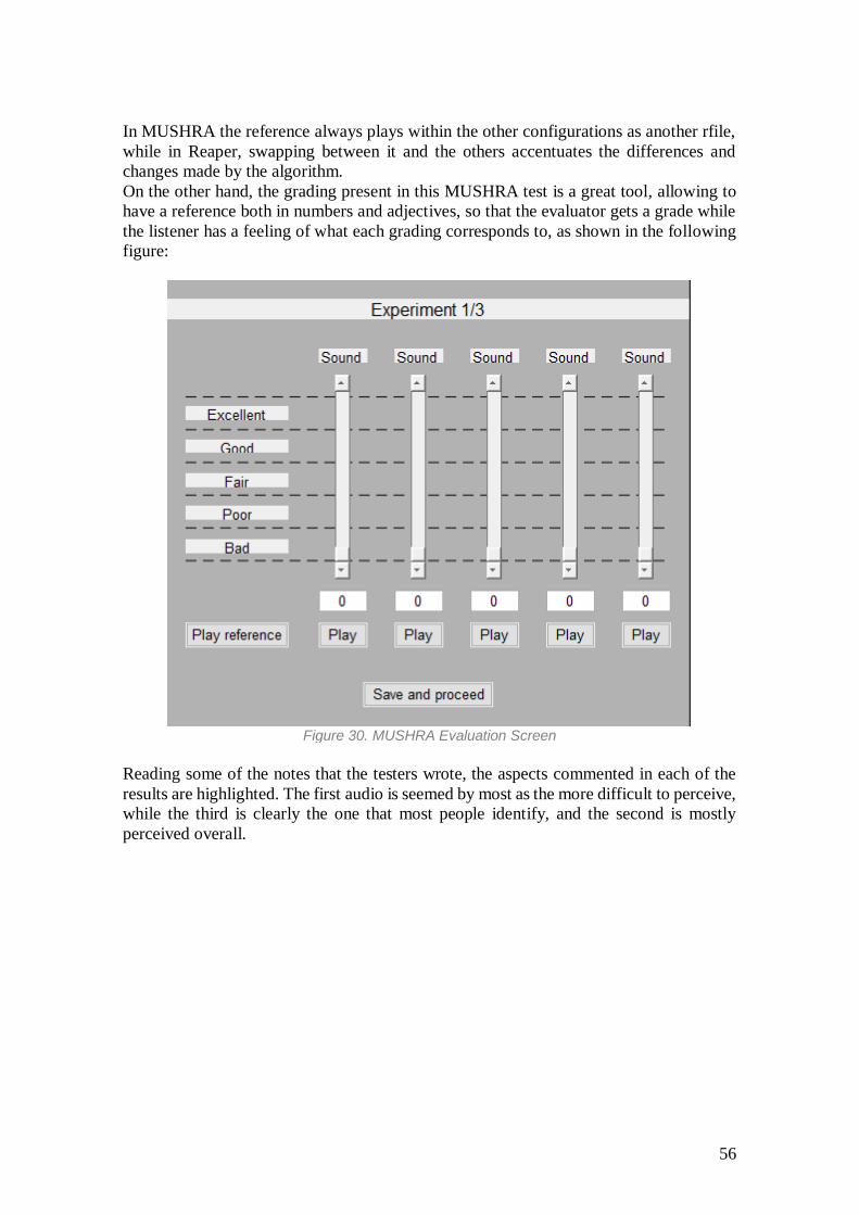
On the other hand, the grading present in this MUSHRA test is a great tool, allowing to
have a reference both in numbers and adjectives, so that the evaluator gets a grade while
the listener has a feeling of what each grading corresponds to, as shown in the following
figure:
Figure 30. MUSHRA Evaluation Screen
Reading some of the notes that the testers wrote, the aspects commented in each of the
results are highlighted. The first audio is seemed by most as the more difficult to perceive,
while the third is clearly the one that most people identify, and the second is mostly
perceived overall.
57
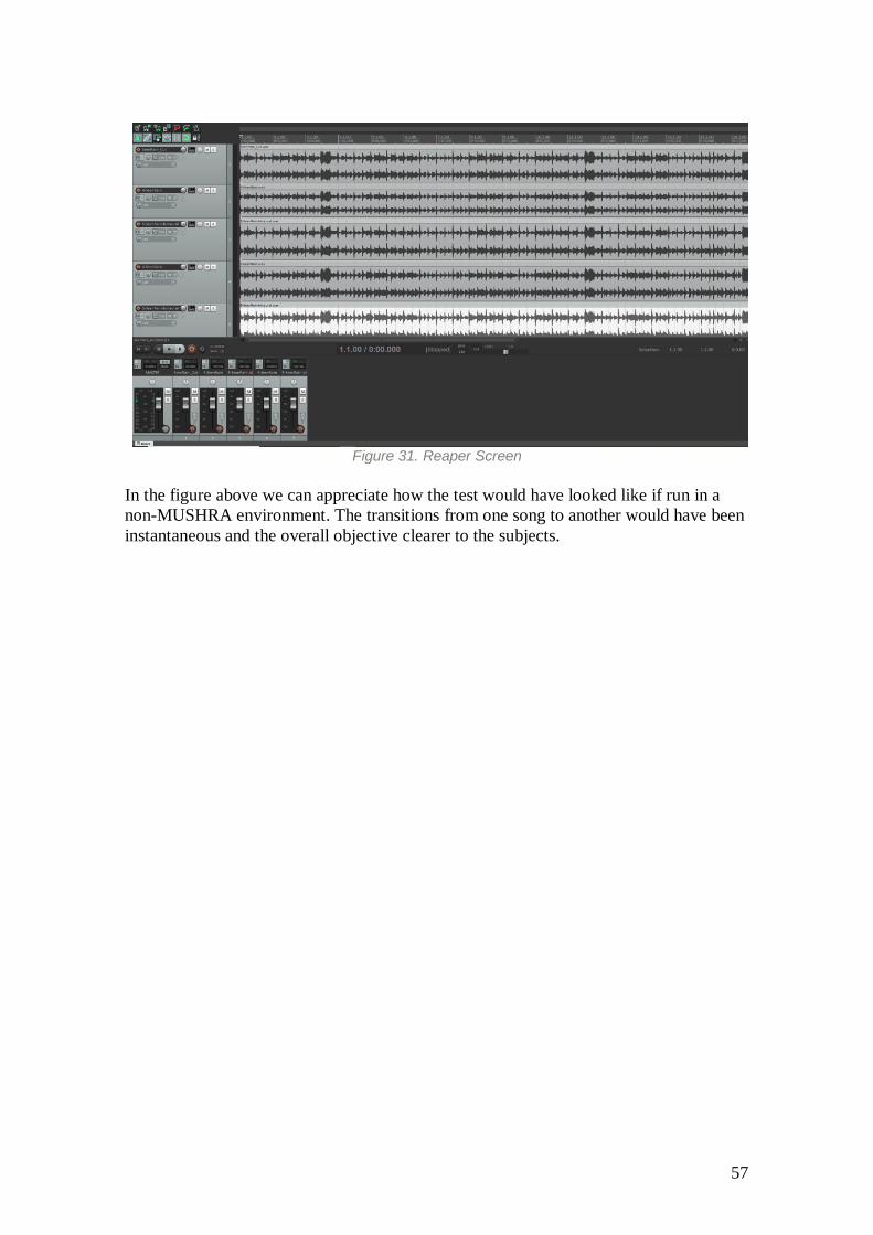
Figure 31. Reaper Screen
In the figure above we can appreciate how the test would have looked like if run in a
non-MUSHRA environment. The transitions from one song to another would have been
instantaneous and the overall objective clearer to the subjects.

58
59
6. CONCLUSIONS & FURTHER WORK As stated in the last point, the algorithm seems to be working but with some drawbacks.
In order to correct these, we believe it would be wise to increase the number of tests
subjects and change the testing environment to that of audio production applications.
Other than that, the fact that our implementation of the algorithm cannot be tested against
another implementation is kind of an issue, but we believe it to be solid. The main reason
we say this is because summing the direct and ambience components of one file results
in a perfect reconstruction of the original audio before the analysis.
Looking back at the results and the comments of the testers, we can conclude that in order
to obtain a more immersive 3D audio space, the virtual sources need to have their own
space without overlapping themselves, as the chaos it ensues works against our objective.
Also, eventhough we selected the equal ratios method because it seemed better, the tests
have shown that in some cases the original stereo was graded almost as some of the
configurations, leading us to believe that both methods should be tested in future essays.
Furthermore, the tests showed that in some cases the HRTFs from the dummy heads, even
being so reliable, were worse graded in some cases. As such, further HRTFs should be
tested to have a more stable response.
We tried to test the performance of the method on different audio files, so that the
robustness of it was put to trial. Just as the resulst have shown, the combination of the
configuration with the different HRTFs makes it a viable method for most generes.
Regarding the future of the algorithm there are some things that can be made to improve
it.
First, some other new configurations could be implemented, so that a more surrounding
or better mix could be achieved. In order to work though, we most likely would have to
apply some other techniques leading to a multichannel approach rather than binaural.
The other main upgrade we would like to do is to have a real time functioning version of
the algorithm, that could run like a plugin. To do so, we would have to work in a C++
implementation of the method.
This real time implementation could be upgraded even further, creating an extension for
web browser such as chrome or firefox. In order to do so, some aspects of the code would
need improvement to make it more efficient.
Finally, we would like to acknowledge this implementation as the first upmix algorithm
that uses the pysofaconvention, proving that SOFA is a whorty standard.

60
61
7.BIBLIOGRAPHY
[1] J. Merimaa, M. M. Goodwin, and J.-M. Jot, “Correlation-Based Ambience Extraction from Stereo
Recordings,” AES 123rd Conv., pp. 1–15, 2007.
[2] C. Avendano and J. M. Jot, “FREQUENCY DOMAIN TECHNIQUES FOR STEREO TO
MULTICHANNEL UPMIX,” 2002.
[3] C. Avendano, “FREQUENCY-DOMAIN SOURCE IDENTIFICATION AND MANIPULATION
IN STEREO MIXES FOR ENHANCEMENT, SUPPRESSION AND RE-PANNING
APPLICATIONS,” 2003.
[4] M. M. Goodwin and J.-M. Jot, “PRIMARY-AMBIENT SIGNAL DECOMPOSITION AND
VECTOR-BASED LOCALIZATION FOR SPATIAL AUDIO CODING AND ENHANCEMENT.”
[5] C. Faller and J. Breebaart, “Binaural Reproduction of Stereo Signals Using Upmixing and Diffuse
Rendering.”
[6] “Introduction to Psychoacoustics - Module 07A.” [Online]. Available:
http://acousticslab.org/psychoacoustics/PMFiles/Module07a.htm. [Accessed: May-2019].
[7] D. Madole and D. Begault, “3-D Sound for Virtual Reality and Multimedia,” Comput. Music J.,
vol. 19, no. 4, p. 99, 1995.
[8] A. Piegari and S. Ausili, “Desarrollo de dispositivo electrónico de bajo costo para evaluar
localización de fuentes sonoras,” 2017.
[9] D. Moore, “The development of a design tool for 5-speaker surround sound decoders,” 2009.
[10] “Perception Lecture Notes: Auditory Pathways and Sound Localization.” [Online]. Available:
https://www.cns.nyu.edu/~david/courses/perception/lecturenotes/localization/localization.html. [Accessed: May-2019].
[11] M. Moradi, “Audio Principles,” 2019. [Online]. Available:
https://www.slideshare.net/mohsenirib/audio-principles-128102222. [Accessed: Jun-2019].
[12] P. Sandgren, S. Examiner, E. Karlsson, and P. Händel, “Implementation of a development and
testing environment for rendering 3D audio scenes,” 2019.
[13] “Neumann KU100 Micrófono Estéreo Binaural | Gear4music.” [Online]. Available:
https://www.gear4music.es/es/PA-DJ-and-Iluminacion/Neumann-KU100-Microfono-Estereo-
Binaural/1BGY. [Accessed: Jun-2019].
[14] C. Pike, “BBC - Research and Development: Listen Up! Binaural Sound,” 2013. [Online].
Available: https://www.bbc.co.uk/blogs/researchanddevelopment/2013/03/listen-up-binaural-
sound.shtml. [Accessed: Jun-2019]. [15] “Mono vs Stereo - Difference,” 2017. [Online]. Available: https://difference.guru/difference-
between-mono-and-stereo/. [Accessed: Jun-2019].
[16] “Loudness Concepts & Panning Laws.” [Online]. Available:
http://www.cs.cmu.edu/~music/icm-online/readings/panlaws/. [Accessed: 09-Jun-2019].
[17] “Ayuda en compra de un home cinema,” 2018. [Online]. Available:
http://www.mundodvd.com/ayuda-compra-de-home-cinema-146253/. [Accessed: Jun-2019].
[18] “‘Convolution,’” Wikipedia: The Free Encyclopedia, Wikimedia Foundation Inc. for publisher,
2019. [Online]. Available: https://en.wikipedia.org/wiki/Convolution. [Accessed: 15-May-2019].
[19] “‘Cros-Correlation,’” Wikipedia Free Encycl. Wikimedia Found. Inc. Publ., pp. 2019-05–15, 2019.
[20] “‘Autocorrelation,’” Wikipedia Free Encycl. Wikimedia Found. Inc. Publ., 2019.
[21] P. Majdak, Y. Iwaya, R. Nicol, M. Parmentier, and F. Televisions, “Spatially Oriented Format for
Acoustics: A Data Exchange Format Representing Head-Related Transfer Functions,” 2013. [22] “SOFA (Spatially Oriented Format for Acoustics) - Sofaconventions.” [Online]. Available:
https://www.sofaconventions.org/mediawiki/index.php/SOFA_(Spatially_Oriented_Format_for_
Acoustics). [Accessed: May-2019].
[23] A. Pérez López, “pysofaconventions,” 2019. [Online]. Available:
https://github.com/andresperezlopez/pysofaconventions. [Accessed: May-2019].
[24] Y. Sánchez Guzmán, “GitHub YeraySG,” 2019. [Online]. Available: https://github.com/YeraySG.
[25] E. Vincent, “MUSHRAM: A MATLAB interface for MUSHRA listening tests,” 2005. [Online].
Available: http://www.elec.qmul.ac.uk/people/emmanuelv/mushram/.
[26] J. Fire, Jambú, Nacional Records. 2017.
[27] B. M, Have You Ever Seen The Rain, Love For Sale, Atlantic Hansa. 1977.
[28] M. Gordon, Rip & Tear, Doom (Original Game Soundtrack), Bethesda Softworks. 2016. [29] “REAPER | Audio Production Without Limits.” [Online]. Available: https://www.reaper.fm/.

62
[Accessed: 15-May-2019].