Embed Size (px)
Citation preview

Steering via Algorithmic Recommendations
Nan Chen Hsin-Tien Tsai∗
May 2021
Abstract
This paper studies whether market structure affects algorithmic recommenda-tions in dominant platforms. We focus on the dual role of Amazon.com—as aplatform owner and retailer. We find that products sold by Amazon receive sub-stantially more “Frequently Bought Together” recommendations across productcategories and popularity deciles. To establish causality, we exploit within-product variation generated by Amazon stockouts. We find that when Amazonis out of stock, for the identical product sold by third-party sellers, the prob-ability of receiving a recommendation decreases by 8 percentage points. Thepattern can be explained by economic incentives of steering and cannot beexplained by consumer preference. Furthermore, the steering lowers recom-mendation efficiency.
Keywords: Product recommendation; vertical integration; e-commerce; digitalplatform; algorithmic bias; big data
JEL Code: D22, D43, L11, L81
∗Chen: Department of Information Systems and Analytics, National University of Singapore,[email protected]. Tsai: Department of Economics, National University of Singapore, [email protected]. For their helpful comments, we thank Zarek Brot-Goldberg, David Byrne, JunhongChu, Andrew Rhodes, Joel Waldfogel, Julian Wright, and seminar participants at the National Uni-versity of Singapore, the National Taiwan University, the 12th World Congress, the University ofMelbourne, Toulouse School of Economics, SKK GSB, Applied Economics Workshop, 14th DigitalEconomics conference, Economics of Platforms Seminar and 19th Annual International IndustrialOrganization Conference. We thank Lee Wei Qing and Zhang Hui for their superb research as-sistance. This research had financial support including the tier 1 research grant and the start-upresearch grant at National University of Singapore.
1

1 Introduction
Algorithmic recommendations are a major information intermediation tool and are
penetrating to people’s social and economic lives. Four in five movies watched on
Netflix came through recommendations and the remaining one from search (Gomez-
Uribe and Hunt, 2016). Besides, large internet platforms (e.g., Amazon, Facebook,
Google) have a dual role, as information intermediaries and players in the related
markets. This market structure—i.e., the dual role—may incentivize platforms to
steer consumers by providing recommendations that favor the information gatekeepers
and are sub-optimal for consumers.1 The concern of steering is especially relevant in
the context of dominant platforms (e.g., Cremer et al., 2019 and Scott Morton et al.,
2019).
Empirical evidence on steering in product recommendation is limited.2 Algo-
rithms are proprietary information unobserved to the public, and more importantly
it is challenging to establish causality. This paper proposes a unique research design
that leverages high-frequency variation in market structure and product recommen-
dations. We provide novel causal evidence that a dominant digital platform’s dual
role can affect the behavior and quality of product recommendation.3
Our empirical context is a dual-role platform—Amazon.com (hereafter Amazon).
1Platform’s dual role may bias information intermediation and has raised regulatoryconcerns. Early examples include “display bias” in the vertically integrated ComputerReservation System in the US airline industry (see https://www.federalregister.gov/
documents/2004/01/07/03-32338/computer-reservations-system-crs-regulations).More recently, Google is accused of “search ranking bias,” i.e., favoring theirown affiliations (see https://www.ftc.gov/news-events/press-releases/2013/01/
google-agrees-change-its-business-practices-resolve-ftc for the US and https:
//ec.europa.eu/competition/elojade/isef/case_details.cfm?proc_code=1_39740 for theEU).
2For diagnoses of search ranking bias, see Edelman (2011). Recent theoretical work includeintermediation with search diversion (e.g., Hagiu and Jullien, 2011; De Corniere and Taylor, 2014;Burguet et al., 2015) and with biased recommendations (e.g., Burguet et al., 2015; De Corniere andTaylor, 2019; Teh and Wright, 2020).
3To the best of our knowledge, the closest empirical work are Aguiar and Waldfogel (2018) andMcManus et al. (2020). Aguiar and Waldfogel (2018) quantify the impact of product recommenda-tions on demand for music and consider “home bias.” McManus et al. (2020) study how an internetservice provider uses nonlinear pricing strategies to steer consumers to more profitable options.
2

Amazon accounts for nearly half of the US e-commerce market (see Section 2). Ama-
zon owns the marketplace and guides consumers using product recommendations.
It is estimated that 30% of page views on Amazon are through recommendations
(Sharma et al., 2015). At the same time, Amazon also sells products directly and
competes with other sellers for consumer demand. Amazon faces a tradeoff between
earning higher retailing profits from products sold by itself and earning lower referral
fees from products sold by other sellers. A profit-maximizing recommendation may
differ from the product consumers like the most, leading to incentives to steer.
We focus on an iconic type of product recommendations called “Frequently Bought
Together” (hereafter FBT). Each product can recommend up to two products as
FBTs. Amazon chooses which products to recommend. We study the recommenda-
tions received by a particular product, which we term “FBTs Received,” as well as
the recommendations initiated by a particular product, which we term “FBTs Ini-
tiated.” Based on massive amounts of choice data and a focal consumer’s current
product choice, FBT recommends to the consumer one or two products that she may
be interested in buying together with her chosen product (see Figure 1(a)).4 FBT
defines a directional pairwise relation between products and provides rich variations
for our analysis.
We construct a unique dataset using public data disclosed by Amazon. We have
information on over 6.7 million products, the near universe of economically significant
products with public data (i.e., as measured by whether the number of customer
reviews is greater than 100). We conducted five rounds of data collection where we
monitored the platform’s assignment of FBT recommendations for the 6.7 million
products. The median time gap between two consecutive rounds is 10 days. We
complement this data with other high-frequency data on product prices and sales to
account for other changes in the markets.5
4FBTs are based on item-to-item relations and are not based on individual consumer’s choicehistory; Section 2.2 provides more discussion.
5We measure product prices using the lowest market prices excluding shipping costs. We ap-proximate sales using sales rank (e.g., Chevalier and Goolsbee, 2003; Chevalier and Mayzlin, 2006).
3
(a) Example of “Frequently Bought Together” Recommendations
(b) Third-Party Product (c) Amazon Product and Amazon Stockout
Figure 1: “Frequently Bought Together,” Product Types, and Amazon Stockout
Note: Figure 1(a) shows an example of Amazon’s FBT recommendations on Marketplace. Thefirst product, termed “Referring Product,” is the product listed on the current product page. Thesecond and third products, termed “Recipient Products,” are the products recommended by the FBTrecommendation. FBT recommendations are made for a specific product, not for a specific seller.Figure 1(b) shows an example of a non-Amazon-selling product (third-party product for brevity);Amazon is not a seller in these markets. Figure 1(c) shows an example of an Amazon-selling product(Amazon product for brevity); Amazon and third-party sellers sell the same product listed on thesame product page. When Amazon is out of stock, only third-party seller’s offers are available.
4
We begin with a descriptive regression analysis of cross-product variations (see
Figure 1 for definitions of Amazon product and third-party product). Conditional
on product price and popularity, Amazon products are 23.6% more likely to receive
FBT recommendations. Meanwhile, Amazon products are only 5% more likely to
initiate FBT recommendations. The gap in the FBTs Received and the FBTs Ini-
tiated is systematic and robust to all deciles of product popularity. Notably, the
gap is substantial among popular products; Amazon products in the top popularity
decile received 3.42 (90.1%) more FBTs than third-party products in the same decile.
The advantage in FBT recommendations enjoyed by Amazon products is remarkably
consistent across product categories.
Comparisons across products are subject to concerns about missing variables.
Exogenous variations on market structure are difficult to obtain.6 Our “big data”
has a major advantage over small data: it allows us to observe rare events — such as
Amazon stockouts — that give us high-frequency within-product variation in market
structure to establish causality. We show that stockout events are plausibly exogenous
as product prices and sales are relatively smooth before the stockouts. At the same
time, we control for real-time prices and sales in our models. The research design
requires that the same recipient product is available from third-party sellers when
Amazon stocks out, therefore we focus on product markets where both third-party
sellers and Amazon are sellers as in Figure A.2(b).7 Products where Amazon is the
sole seller (e.g., Amazon private-label products) do not meet this condition and are
not included in the within-product analysis.8
When Amazon experiences a stock out, we find that an 8 percentage point decrease
6For a recent empirical evaluation of vertical integration with causal identification, see Luco andMarshall (2020).
7For simplicity, we refer to these Amazon-selling markets (products) as “Amazon markets (prod-ucts).” These Amazon markets have Amazon as a seller and can have third-party sellers. We referto markets where Amazon is not a seller as “third-party markets.”
8Amazon’s private-brand sales represent only 1% of Amazon’s first-party sales(see page 24 in https://docs.house.gov/meetings/JU/JU05/20200729/110883/
HHRG-116-JU05-20200729-QFR052.pdf).
5

in the probability of receiving a recommendation for the same recipient product sold
by third parties. Importantly, we account for consumer preferences by controlling for
real-time prices and sales. Using the estimates on price and sales as a benchmark,
we show that a 20% change in price or popularity will only change the probability of
receiving a recommendation by 0.3 percentage points. Our results are robust under
alternative model specifications and placebo tests. By performing sensitivity tests
that manually add large hypothetical measurement errors in price and sales, we show
that the confounding factors need to be very strong in order to explain our result;
artificially making third-party products 100% more expensive or making Amazon-
selling products 100% more popular cannot explain our finding on steering.
We conduct further analysis to rule out alternative interpretations. First, for the
same directional FBT pair, Amazon stockouts in a referring product market decrease
the probability of initiating FBTs by only 0.1 percentage points. Second, Amazon
products are favored relative to “Fulfillment By Amazon” (FBA) products, which are
similar to Amazon products in shipping and services. Third, we repeat the analysis
using the same research design and find that the variations in third-party sellers’
presence have no significant effect on FBT. Overall, the evidence supports that the
effect is driven by seller identities rather than omitted confounding shocks in supply
or demand. We therefore argue that the steering behavior of the FBT algorithm is
not driven by consumer preference.
Next, we show that steering can be explained by Amazon’s economic incentives.
We use a simple linear model to quantify the effectiveness of FBT, i.e., the degree to
which FBT recommendations translate into sales. For the same pair of referring and
recipient products, our model quantifies how the correlation of their sales responds
to the change in FBT. We estimate the effectiveness of FBT in each of the largest 30
product categories. We find that Amazon employs more steering in categories where
FBTs are more effective. We present two additional observations that are consis-
tent with Amazon’s economic incentives to steer: (i) the more popular the referring
6

product, the higher the likelihood of steering; and (ii) products that make zero or
one recommendation, the estimated FBT effectiveness is zero, as is the estimated
likelihood of steering.
Lastly, we test whether the steering decreases the overall effectiveness of FBT rec-
ommendations. We compare the effectiveness of four types of FBT pairs: (i) Amazon
to Amazon; (ii) Amazon to third party (iii) third party to Amazon; and (iv) third
party to third party. We construct matched balanced panels to facilitate the compar-
isons across FBT pairs. If FBTs favor Amazon products over alternative third-party
products, then Amazon recipient products may on average be a worse fit in terms of
consumer preference. Consistent with the prediction, we find that recommendations
directing consumers to Amazon products are significantly less effective. The results
reinforce our results on steering and imply that the steering driven by a platform’s
dual role can potentially hurt consumers and third-party sellers.
To summarize, we provide novel causal evidence on algorithmic steering in prod-
uct recommendation. Large internet platforms are information gatekeepers in many
sectors of the economy. Information intermediation through algorithmic recommenda-
tions is increasingly important to platform businesses and social welfare. Our results
suggest that market structure affects the behavior and quality of product recommen-
dations. Given the black-box nature of algorithms to the public (and sometimes even
to the firm itself), our results raise concerns over the market’s ability to detect and
correct potential algorithmic bias. More attention and discussions on competition
policy and algorithmic accountability seem necessary (e.g., Cremer et al., 2019 and
Scott Morton et al., 2019).
1.1 Related Literature
This paper contributes to several strands of literature. First, Amazon’s dual role can
be seen as a type of vertical integration. This paper is related to extensive theoretical
and empirical work on the potential anticompetitive effects of vertical integration.
7

Prior work have empirically studied industries include traditional retailing such as
yogurt (Berto Villas-Boas, 2007), beer (Asker, 2016), and carbonated-beverage (Luco
and Marshall, 2020), cable television (e.g., Waterman and Weiss, 1996; Chipty, 2001;
Crawford et al., 2018), gasoline (e.g., Hastings and Gilbert, 2005; Houde, 2012), con-
crete (e.g., Hortacsu and Syverson, 2007), electricity (e.g., Bushnell et al., 2008),
video game (e.g., Lee, 2013), production (e.g., Atalay et al., 2014), residential broker-
age (e.g., Barwick et al., 2017), health care (e.g., Brot-Goldberg and de Vaan, 2018),
and telecommunications (e.g., McManus et al., 2020). Our paper focuses on a digital
platform, namely Amazon Marketplace (Zhu and Liu, 2018). We document novel
empirical evidence on algorithmic steering in product recommendations, which can
be seen as a special form of market foreclosure.
Second, this paper relates to empirical studies on digital platform’s information
intermediation using tools such as recommender systems (e.g., Sharma et al., 2015;
Aguiar and Waldfogel, 2018) and search design (e.g., Dinerstein et al., 2018). Edel-
man (2011) discusses the identification and measurement of biased search ranking by
a major search platform. We focus on algorithmic steering using product recommen-
dations. More broadly, our paper relates to the current discussion on algorithmic
biases (e.g., Mullainathan and Obermeyer, 2017; Obermeyer et al., 2019; Cowgill and
Tucker, 2020; Rambachan et al., 2020). We highlight the role of developers’ economic
incentives in affecting algorithmic behaviors and show that social welfare may not be
maximized in recommendation systems (e.g., Bergemann et al., 2019).
The rest of this paper is organized as follows. Section 2 provides an overview
of the empirical context and institutional background. Section 3 describes the data.
Section 4 and Section 5 examine the relation between seller identity and algorithmic
recommendations. Section 4 uses cross-product variations and Section 5 uses within-
product variations. Section 6 discusses the extent to which steering can be explained
by a simple economic incentive — profit maximization. Section 7 provides evidence
8

on inefficient recommendations due to the steering. Section 8 concludes. Additional
results and robustness checks are in the appendices.
2 Amazon Marketplace
Today, online commerce saves customers money and precious time. To-
morrow, through personalization, online commerce will accelerate the very
process of discovery.
— Bezos (1997), Letter to Shareholders
For two decades now, Amazon.com has been building a store for every
customer. Each person who comes to Amazon.com sees it differently,
because it’s individually personalized based on their interests. It’s as if
you walked into a store and the shelves started rearranging themselves,
with what you might want moving to the front, and what you’re unlikely
to be interested in shuffling further away.
— Smith and Linden (2017), Two Decades of Recommender Systems at
Amazon.com
2.1 Market Structure
Amazon Marketplace is one of the world’s leading digital platforms. Amazon.com
is the largest e-commerce platform in the U.S.; it was about six times the size of
its closest competitor in 2018, and is expected to grow bigger).9 According to the
9According to an earlier estimate by eMarketer, Amazon accounted for 47% ofU.S. total online retail sales in 2018. Following a public disclosure by Bezos (2018),eMarketer revised their estimate to 38% (https://www.statista.com/chart/18755/amazons-estimated-market-share-in-the-united-states/; https://www.bloomberg.com/
news/articles/2019-06-13/emarketer-cuts-estimate-of-amazon-s-u-s-online-market-share).The estimate of 38% is considered conservative. As of 2020, Bank of Amer-ica estimates Amazon’s market share to be 44% (https://finance.yahoo.com/news/latest-e-commerce-market-share-185120510.html) while Statista
9

U.S. Census Bureau, total e-commerce sales in the U.S. was $513 billion in 2018.10
According to Bezos (2018), Amazon’s total sales in 2018 amounted to $277 billion,
of which 58% or $160 billion were accounted for by third-party sellers. Amazon Mar-
ketplace has allowed independent third-party sellers to sell products on its platform
since 2000.11 Third-party sellers are mostly small- and medium-sized businesses. As
of 2020, Amazon Marketplace has 8.9 million sellers worldwide, of which 2.3 million
are active sellers with product listings.12
Amazon Marketplace lists hundreds of millions of products (Smith and Linden,
2017). The products in the Marketplace are precisely identified using a unique number
called “Amazon Standard Identification Number” (ASIN).13 Each product market can
have one of three types of market structure depending on the composition of sellers:
“Amazon-only,” “Amazon and third-party,” and “third-party-only.” “Amazon-only”
refers to markets where Amazon is the only seller; “Amazon and third-party” refers
to markets where both Amazon and third-party sellers are selling the product; and
“third-party-only” refers to markets where only third-party sellers are selling the
product. Both “Amazon only” and “Amazon and third-party” are considered to
be “Amazon markets.” Table 1 shows the frequency of the three types of market
structure in our data.
In “third-party-only” markets, Amazon receives commission fees of around 15%
estimates it to be 47% (https://www.statista.com/statistics/788109/amazon-retail-market-share-usa/). Amazon’s closest e-commerce competitor is e-Baywith a share of 6.6% (eMarketer’s 2018 estimate; https://techcrunch.com/2018/07/13/
amazons-share-of-the-us-e-commerce-market-is-now-49-or-5-of-all-retail-spend/)and Walmart with a share of 7% (Bank of America’s 2020 estimate).
10https://www2.census.gov/retail/releases/historical/ecomm/18q4.pdf.11For comments on the decision to allow third-party sellers to sell on the marketplace, see Bezos
(2005).12https://www.marketplacepulse.com/amazon/number-of-sellers.13For instance, there is a unique ASIN for “Samsung Galaxy Note 10 Lite N770F 128GB Dual-SIM
GSM Unlocked Phone (International Variant/US Compatible LTE) – Aura Black.” See https://
www.amazon.com/N770F-Dual-SIM-Unlocked-International-Compatible/dp/B084MDBXRD. TheASIN is remarkably precise; the Aura Glow version of the same phone has a different ASIN. OnSeptember 23, 2020, three third-party sellers were selling the product, at prices of $433.00, $433.99,and $434.00, respectively. The shipping cost was zero for all three sellers when we set the zip codeat 94704 (Berkeley, CA).
10

of the revenue. In Amazon-only markets, Amazon receives 100% of the revenue. In
“Amazon and third-party” markets, Amazon’s revenue depends on how often Amazon
is featured as the default seller in “Buy Box.” Currently, regulators (e.g., EU Com-
mission, 2020) focus on Amazon’s steering using Buy Box, which steers consumers
towards a “seller.” This paper focuses on steering using FBT, which steers consumers
toward a “product.” Amazon and third-party sellers compete to “win” the Buy Box
listing. The Buy Box algorithm is determined by Amazon (and is held constant in
this study). We use a sample of 1.3 million Buy Box observations of “Amazon and
third-party” markets. Amazon wins 63.8% of Buy Box listing. As an approximation,
Amazon may take 70% ≈ 100%∗63.8%+15%∗(1−63.8%) of the revenue in “Amazon
and third-party” markets.
Panel A in Table 1 shows that Amazon is the only seller in 4.2% of all product
markets.14 Amazon and third-party markets account for 14.5% of markets, and third-
party-only markets account for 81.3%. Panel B in Table 1 shows the same statistics
for the set of products that receive or initiate at least one FBT recommendation.
These products, which we refer to as “FBT products,” are the focus of our analysis.
There are 4.1 million FBT products accounting for 61.2% of all products in our data.
The share of Amazon markets is slightly higher, especially for “Amazon and third-
party markets,” which account for 19.1% of all product markets measured by the
number of products.
2.2 Frequently Bought Together
Recommender systems are important to the digital economy and in particular to
the e-commerce ecosystem. A Microsoft Research report estimated that 30 percent
of Amazon.com’s page views are based on recommendations (e.g., Sharma et al.,
2015; Smith and Linden, 2017). Amazon is one of the pioneers in recommender
14Appendix A conducts analysis separately for these Amazon-only markets and the results aresimilar.
11

systems. Like other large Internet platforms, Amazon collects data on activities in
the marketplace. Recommender systems can learn about consumers’ preferences from
consumer choice data and then provide personalized information to consumers. These
systems can reduce search frictions and increase matching qualities (e.g., Bergemann
and Bonatti, 2019).
This paper focuses on Amazon’s classic “Frequently Bought Together (FBT)”
recommendations. FBT recommendations are made for a specific product, not for
a specific seller. As the name suggests, FBT recommendations attempt to predict
which products a consumer might be interested in buying based on the current prod-
uct she is selecting. By using real-time information on consumers’ current choices
and offering FBT recommendations, the algorithm can personalize information and
facilitate product discovery. The recommended products are often complementary to
the current chosen product. The FBT recommendations are displayed on the refer-
ring product page (see Figure 1(a)). Amazon decides which products to recommend;
third-party sellers have no control over the recommendations. Third parties can buy
sponsored recommendations from Amazon. FBT recommendations are considered
as “organic” non-sponsored recommendations that are driven by consumer demand.
Specifically, it is believed that FBT recommendations are based on the Item-to-Item
Collaborative Filtering, which was first launched by Amazon in 1998 (Linden et al.,
2003). The algorithm has been used by many websites including YouTube, Netflix,
and Google News.
Amazon also has other onsite recommendations such as “Recommended for You,”
“Featured Recommendations,” “Customers who bought this item also bought,” and
“Customers who viewed this item also viewed,” as well as sponsored recommenda-
tions such as “Sponsored products related to this item.” FBT is special in several
aspects. First, it is more integrated into the consumer buying process; customers can
add with one click all FBT-recommended products to their carts, or select a specific
product that they wish to purchase. Second, Amazon constrains the number of FBT
12

recommendations initiated by a product. A product can make at most two recom-
mendations. Table 3 summarizes the distribution of the number of recommendations
initiated with each product in the data. Third, some recommendations such as “Rec-
ommended for You” can be based on an individual consumer’s choice history. FBT
recommendations are easier to decipher; FBTs are based on item-to-item relations
and are not based on individual consumer’s choice history.
While concepts related to algorithmic recommendations (e.g., data mining, ma-
chine learning) may sound neutral, the key parameters and objective functions of
algorithms are chosen by human managers or developers.15 Whether Amazon’s dual
role affects algorithmic recommendations is particularly unclear since the company is
widely recognized for its forward-looking strategy and its willingness to forgo short-
run profits.16 Our assessment of the degree to which a customer-centric firm engages
in steering informs the broader policy discussion.
3 Data
Our data cover over 6.7 million products listed on Amazon.com. To capture platform-
level recommendation flows, we focus on economically significant products. Amazon
does not disclose the absolute level of sales, so we use the number of customer reviews
as a proxy. The assumption is that the total number of units sold of a product is
correlated with the number of customer reviews. We cover the near universe of
products with at least 100 customer reviews. We do not have data on e-books because
15Algorithms may not be transparent even to their developers. For recent perspectives,see Cowgill and Tucker (2020). For policy discussions, see https://www.congress.gov/bill/
116th-congress/house-bill/2231/all-info for the US and https://www.europarl.europa.
eu/RegData/etudes/STUD/2019/624262/EPRS_STU(2019)624262_EN.pdf for the EU.16The strategy has been central in Amazon’s message to its investors since 1997 (e.g., Bezos,
1997, 2017). The company’s stated mission is to be “Earth’s most customer-centric company” (e.g.,https://www.amazon.jobs/en/working/working-amazon). See also Khan (2016).
13

public data are unavailable. Overall, our data are comprehensive at the platform
level.17
For each product market, we record the market price, defined as the lowest price
among all the sellers including Amazon. Market prices do not include shipping costs.
We also record each product’s historical sales ranking, which is the relative ranking
of a given product’s sales within its product category. This measure has been used
as a proxy for product sales, as previous work suggests that the log transformation of
sales rank has an approximately linear relation with the log transformation of sales
(Chevalier and Goolsbee, 2003; Chevalier and Mayzlin, 2006). Our price and sales
data are measured at a daily frequency. The high frequency allows us to control for
real-time changes in the markets.
Additionally, our data also record the number of sellers in each product market.
This information allows us to identify when a seller enters a given product market;
that is, the number of offers increases by one when an additional seller enters the
market. This data will be used to (i) identify variations in third-party seller presence;
and (ii) construct matched samples when we study the recommendation efficiency
across FBT types. We also have basic information about all products including their
corresponding product categories such as Bedding, Kitchen & Dining, and so on. The
product category information will allow us to control for category-date level trends
and conduct cross-category analyses.
For the full set of products, we construct another high-frequency dataset for Fre-
quently Bought Together product recommendations. We keep track of Amazon’s
assignment of FBTs for five rounds from December 2019 to February 2020. The me-
dian time gap between the two rounds is 10 days. In each round and for each product,
we identify the recipient products recommended with the focal referring product to
construct a large-scale picture of the FBT recommendation flows among the 6.7 mil-
17Products that are newly introduced may be less likely to be included in our data. This is lessof a concern for our purpose.
14

lion products. Note that we do not observe the FBT recommendation received from
outside of our 6.7 million products.
Table 2 shows the summary statistics at the product level. The table uses data
from the first round of data collection. Panel A of Table 2 shows the full sample
for all the 6.7 million products. The average market price of a product is $40.54.
The average sales rank of a product is about 931,807. We study both the number of
recommendations received by a particular product, which we term “FBTs Received,”
as well as the number of recommendations initiated by a particular product, which
we term “FBTs Initiated.” The average number of FBTs Received is 0.68 while the
average number of FBTs Initiated is about 0.91.
Panel B of Table 2 shows the summary statistics of products that receive or initiate
at least one recommendation over the sample period. The average market price is
$34.00 and the average sales rank is 548,296. The FBT products are on average
relatively cheaper and more popular than the full sample of products. The average
number of FBTs Received is 1.12, while the average number of FBTs Initiated is
about 1.49.
Table 3 shows the distribution of FBTs Received and FBTs Initiated from the
first round of data collection. As in Panel A, 84.4% of the full set of products did
not receive any recommendations. The majority of the remaining products received
between one and three recommendations. Around 2.5% of products receive more
than five recommendations. For FBTs Initiated, 40.6% of products do not initiate
any recommendations; 27.4% of products use only one of its two recommendation
slots; 32% of products use both recommendation slots. Panel B summarizes the FBT
flows for FBT products, i.e., products that were referring products, recipient products,
or both. Only 3.3% of products do not initiate any FBT recommendations.18 For
FBTs Received, the distribution is relatively similar to Panel A. We observe that
74.6% of FBT products do not receive any FBT recommendations. Most of these
18These products may initiate FBT recommendations in a later round of our data. They mayalso be only FBT recipient products.
15

FBT products serve only as referring products. Figure A.4 shows the FBTs Received
and FBTs Initiated over the five rounds of data collections.
3.1 Within-Product Variations in Recommendation Patterns
and Amazon Presence
Our data contain two sources of within-product variations. First, we record the tem-
porary presence or absence of Amazon’s offer in each product market. The temporary
presence or absence of Amazon’s offer yields variation in market structure that we
will exploit to establish causality. Within a small time window, the temporary vari-
ations of Amazon’s offer are presumably due to Amazon being out of stock for the
product. Overall, we observe a change in Amazon’s offer (i.e., Amazon’s presence)
for about 2.16% of products in our period of study. Figure A.5(a) depicts the varia-
tions in Amazon’s presence over the five rounds of data collection for 1,000 products.
The 1,000 products are randomly sampled from all the products for which there was
a change in Amazon’s presence. Most of the variations in Amazon’s presence are
temporary. Appendix B uses an event study approach to show how the variations
impact the product markets. Prices and sales are relatively smooth before Amazon’s
presence changes, suggesting that events are plausibly exogenous.
The second source of variation is the dynamic patterns of FBT recommendations.
We find that 10.20% of products experienced a change in FBTs Received during our
sample period. In addition, we find that 49.35% of FBT pairs experience changes in
whether the referring product recommends the recipient product over five rounds of
data collection. Figure A.5(b) depicts the variations in FBT recommendation over
the sample period for 1,000 product pairs (pairs of referring product and recipient
product). The 1,000 pairs are randomly sampled from all the pairs that experience
one or more changes in their recommendation patterns.
16

4 Seller Identity and FBT Recommendation: Cross-
Product Evidence
In Section 4, we conduct descriptive analyses on how FBT recommendations corre-
lated with whether Amazon is a seller. FBT defines directional pairwise relations
among the products. This allows us to exploit the directionality of the FBT pairs
by comparing how FBTs Received and FBTs Initiated differ depending on Amazon’s
presence i.e., whether Amazon sells in focal markets. We first examine the patterns in
FBTs conditional on product popularity and product category respectively. We then
use regression analysis to quantify how FBTs Received and FBTs Initiated depend
on seller identity. For our purpose, we focus on the FBT products, which are defined
as those that receive or initiate at least one recommendation in our data.
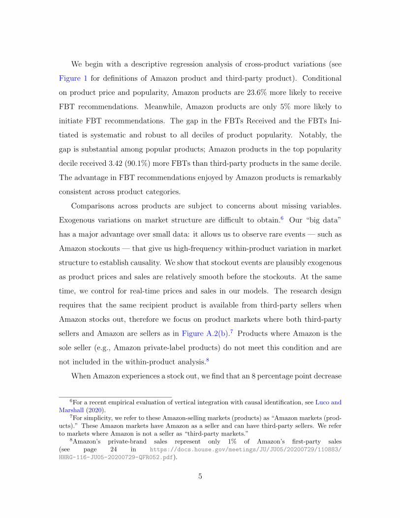
Figure 2 plots the average number of FBTs Received and FBTs Initiated for
Amazon and third-party products conditional on 10 deciles of sales rank. Different
product categories can have a different number of products, and smaller product
categories may have smaller sales ranks. To account for this, we define the deciles
of sales rank within each category. For FBTs Initiated, third-party products initiate
a similar number of recommendations as Amazon products (1.45 versus 1.63). For
FBTs Received, there is a substantial gap in the number of recommendations received
between Amazon products and third-party products. On average, Amazon products
receive 1.55 more recommendations than third-party products (2.34 versus 0.79).
Figure 2 shows that FBTs tend to direct consumers to popular products. The
discrepancy in FBTs Received between Amazon products and third-party products
may be explained by product popularity. To mitigate the confounding effect, we can
directly compare the FBT flows within each decile of sales rank. The difference in
FBTs Received is consistent across sales rank deciles. Amazon products in the first
decile of sales rank receive 7.22 recommendations on average. On the other hand,
17
02
46
8N
umbe
r of
Rec
omm
enda
tions
1 3 5 7 9Sales Rank Decile
FBTs Received: Amazon = 1 FBTs Initiated: Amazon = 1
FBTs Received: Amazon = 0 FBTs Initiated: Amazon = 0
Note: Figure 2 plots the average number of FBTs Received and number of FBTs Initiated forAmazon products and third-party products along with sales rank deciles, respectively. A smallersales rank decile means that the product is more popular. “Amazon=1” indicates Amazon products.“Amazon=0” indicates third-party products.
Figure 2: FBTs Received and FBTs Initiated by Amazon’s Presence and by SalesRank
third-party products in the first decile of sales rank only receive 3.80 recommendations
on average.
Next, we examine the patterns in FBT recommendations across product cate-
gories. Figure A.3 plots the average number of FBTs Received and FBTs Initiated
for Amazon products and third-party products for the top 30 product categories. The
top 30 product categories are all product categories that account for more than 0.5%
of the total FBT pairs in our data.
The patterns are remarkably consistent. Across all product categories, Amazon
products and third-party products are similar in FBTs Initiated. Amazon products
initiated slightly more FBTs on average than third-party products. For FBTs Re-
ceived, Amazon products receive a greater number of FBTs in almost all the product
18

categories. The advantage of Amazon products is the largest in Movies and TV. For
Accessories, Amazon and third-party products have similar FBTs Received.
4.1 Cross-Product Regression Analysis
We use regression analysis to summarize our cross-product analysis. We consider the
following simple specification:
log(Ini + 1) = θ × PLAT Recipienti + γ × log(Q Recipienti)
+ η × log(P Recipienti) + Cat FEi + εi,(1)
where Ini is the number of FBT recommendations that the recipient product i receives.
PLAT Recipienti is an indicator of whether the recipient product i is an Amazon
product. Cat FEi denotes category fixed effects. We sequentially add the log of
recipient product’s market price log(P Recipienti) and the log of recipient product’s
sales log(Q Recipienti) into Equation 1. As mentioned, we approximate the log of
sales using a linear function of the log of sales ranks Rank Recipienti as follows:
log(Q Recipienti) ≈ a+ b log(Rank Recipienti). (2)
For simplicity, we let b = −1. We do not try to estimate the value of b. Note that
a different value of b will simply re-scale the parameter estimates by b. The value of
a is normalized at 0. Note that we allow for category fixed effects in Equation 1. The
fixed effects can be seen as allowing some cross-category heterogeneity in Equation 2.
Table 4 presents the regression results. As in column (4), the coefficient on Ama-
zon products is around 0.24 and statistically significant after we control for both sales
and prices; this implies that conditional on sales and prices, Amazon product is more
likely to receive more recommendations. Comparing column (1) and column (3), the
coefficient on Amazon products decreases after we control for sales. This is consistent
with our previous findings: Amazon products tend to be more popular and popularity
19

can explain some of the differences in FBTs Received. Comparing column (1) and
column (2), the coefficient on Amazon products is not sensitive to the control of price.
We conduct similar regression analysis for the FBTs Initiated:
log(Outi + 1) = θ × PLAT Referringi + γ × log(Q Referringi)
+ η × log(P Referringi) + Cat FEi + εi,(3)
where Outi denotes the number of FBTs Initiated by the referring product i. PLAT Referringi
is an indicator of whether referring product i is an Amazon product. We also sequen-
tially control for the log of referring product’s market price log(P Referringi) and the
log of referring product’s sales log(Q Referringi).
Table A.1 presents the results for FBTs Initiated. As in column (4), the coefficient
on Amazon products is 0.05 after we control for both sales and prices. While the effect
is still statistically significant, it is substantially smaller than the estimate in FBTs
Received.
The reduced-form evidence documents the FBT recommendation patterns at the
platform level. On average, Amazon products receive a greater number of FBT
recommendations. This pattern remains after we control for product prices and sales.
It cannot be fully explained by higher product complementarity for Amazon products,
because the estimate on FBTs Initiated is substantially smaller. However, cross-
product comparisons may suffer omitted variable bias and usually cannot support
causal interpretations. In Section 5, we conduct causal analyses by exploring within-
product variations in Amazon’s temporary presence.
20

5 Seller Identity and FBT Recommendation: Within-
Product Evidence
An information intermediary can maximize consumer surplus by recommending the
product that best fits consumer preference. The fact that Amazon sells some products
may discourage it from recommending the product that a consumer likes the most.
For example, suppose that Amazon’s algorithm identifies two candidate FBT recipient
products that a given consumer may like. Product 1 is sold by both Amazon and third-
party sellers, whereas product 2 is sold by only third-party sellers. For simplicity, we
assume that cost is zero in this case so that revenue equals retail margin. Both
products have the same retail margin of $10. If Amazon recommends product 1, the
consumer buys with a 5% probability, in which case Amazon earns roughly 70% the
whole retail margin (the other 30% may go to competing third-party sellers. See
Section 2.1 for an approximation). If Amazon recommends product 2, the consumer
buys with a 20% probability, in which case Amazon earns only 15% of the retail
margin. To maximize its own profit, Amazon would recommend product 1 because
5%×70%×$10 > 15%×20%×$10, even though the data predicts that the consumer
is three times more likely to prefer product 2.19
For the steering behavior to happen, neither Amazon’s management team nor
its data scientists need to explicitly favor Amazon products. The management team
may simply set (part of) the goal to increase Amazon’s profit. The data science team
then specifies the objective function by choosing the parameters and constraints, and
then trains their models to pick the “best” configuration. If Amazon’s own profit
enters the objective function in some forms, steering may emerge endogenously even
without anyone’s explicit communication or intention. Unlike traditional settings
where pricing and important economic decisions are made by human managers, the
19Appendix C presents a toy model to show that Amazon’s presence can increase the likelihoodof receiving a recommendation.
21
decision process in a recommender system is “outsourced” to potentially black-box
algorithms.
While the intuition above is simple, an empirical test is usually difficult. In
Section 4, we document a substantial gap in FBTs Received between Amazon and
third-party products. We show that the gap is largely consistent across product
categories and sales rank deciles. In Section 5, we go beyond cross-market analysis
and seek a more causal interpretation. To do so, we use Amazon stockout events
that create temporary shocks on Amazon’s incentive to recommend exactly the same
products. In Appendix B, we use an event study approach to show that the stockout
events are plausibly exogenous.
5.1 Main Results
We construct a balanced panel for FBT product pairs. The panel includes all unique
directional FBT pairs if there is ever a recommendation between the referring product
and the recipient product in our data.
As described in Section 3.1, we have within-pair-level variations in FBT recom-
mendation patterns over time. For all the products, we have real-time variations in
Amazon’s presence. For within-product analysis, we focus on Amazon products that
have at least one third-party seller sell the identical products; when Amazon is out of
stock, the product is still listed on the same product page and available for purchase
from third-party sellers. If Amazon is the only seller for a product (e.g., Kindle or
products with “AmazonBasics” branding), the product is not available during Ama-
zon’s temporary absence. We exclude these Amazon-only products so that we do not
capture the impact of product availability on recommendations.
For a given pair of referring-recipient products, we estimate the change in the
22

FBT recommendation depending on whether Amazon sells in the recipient product’s
market. In particular, we examine the regression as follows:
FBTnt = θ × PLAT Recipientnt + γ × log(Q Recipientnt)
+ η × log(P Recipientnt) + Pair FEn + Cat Daynt + εnt,(4)
where n denotes a directional FBT pair of referring product and recipient product.
FBTnt equals 1 for FBT pair n at time t if the referring product recommends the
recipient product at time t and equals 0 otherwise. PLAT Recipientnt is an indicator
of whether Amazon is a seller in the recipient market of FBT pair n at time t.
Pair FEn denotes fixed effects for FBT pair n. Cat Daynt is the category–day fixed
effects for the recipient product of FBT pair n at time t. It controls for category-
specific variations across the calender dates. Q Recipientnt is the log of recipient
product’s sales. P Recipientnt is the log of recipient product’s market price.
In Equation 4, we are interested in the coefficient of PLAT Recipientnt. It mea-
sures the (percentage point) change in the probability of receiving an FBT recommen-
dation depending on temporary variations in Amazon’s presence. After introducing
the model, we highlight a few advantages of our identification. First, our panel model
controls directional FBT pair-level fixed effects. Using only within-product variations
help us rule out a large set of alternative interpretations of our results. These include
concerns that Amazon sells products that are more popular, more recommendable,
or more complementary to other products. As long as these heterogeneous product
characteristics are time-invariant, they are absorbed by directional FBT pair fixed
effects.
Second, our main specification controls for real-time prices and sales. This controls
the dynamics of the demand and supply (e.g., how “likeable” a product is) associ-
ated with Amazon’s temporary absence. Amazon’s absence from a product market
increases its price, and a higher price may make the product less recommendable.
Comparing across the columns of Table 5, we find that the coefficient on Amazon’s
23

presence changes little after controlling for real-time prices (sales), suggesting that
changes in prices (sales) cannot explain the changes in FBT recommendations. An-
other possibility is that the FBT changes are due to the additional shipping costs after
Amazon stocks out while our measurement of price does not include shipping costs.
We address this concern in two ways. First, the number of FBT received decreases
for products sold by FBA sellers, who also provide free shipping (see Section 5.2.2).
Second, we manually make third-party products much more expensive during Ama-
zon’s absence (or Amazon products much more popular during Amazon’s presence).
We find that they explain little of the changes in FBTs (see Section 5.2.3).
Table 5 presents the estimates from Equation 4. Across all specifications, the
coefficient of interest (e.g., PLAT Recipientnt) is around 0.08 and significantly greater
than 0. This suggests that Amazon’s presence (in the recipient product’s market)
increases by 8 percentage points the recipient product’s probability of receiving an
FBT recommendation from the same referring product. The estimates on price and
sales have expected signs: lower prices and higher popularity increase the probability
of being recommended. As shown in column (3) of Table 5, the effect of Amazon’s
presence is substantial comparing to the effects of price and popularity. For a product
with the average price of $34, a 20% increase in its price will decrease the probability
of it being recommended by only 0.25 percentage points=0.014 ×[log(34 × (1 +
20%))− log(34)
]. For a product with the average sales rank of 548,296, a 20%
decrease in its popularity will decrease the probability of it being recommended by
only 0.2 percentage points=0.016×[log(548296× (1 + 20%)
)− log(548296)
]. Taken
together, we conclude that the change in FBT recommendations is driven by whether
Amazon sells in the recipient market.
5.1.1 Robustness Checks
In Appendix D, we conduct three sets of robustness checks.
First, our main model is a linear probability model. We choose it as the main
24

model for its simplicity and transparency. Practically, it is computationally efficient
when we have millions of fixed effects. We test alternative model specifications such
as logit and probit models for binary dependent variables. The results are reported in
Table A.4. As we expect, they predict similar marginal effects and are consistent with
our linear probability model. Second, our main model specification controls for cur-
rent prices and sales. We also test alternative specifications that include lagged sales
and prices. Table A.5 reports the results. Again, our main results are robust. Third,
we conduct standard placebo tests by randomizing the treatments. Within each FBT
pairs, we randomize Amazon’s presence across the different rounds. Table A.6 shows
that placebo Amazon’s presence does not affect FBT recommendations. This exercise
highlights the temporary variations that we use for identification.
5.2 Supporting Results
To strengthen our identification and results, we conduct four additional sets of anal-
yses. We analyze (1) the impact of Amazon’s presence on FBTs Initiated, (2) the
types of the remaining third-party sellers after Amazon’s stockouts, (3) large mea-
surement errors in prices and sales, and (4) the impact of variations in third-party
sellers’ presence. Overall, “competition on the merits” and consumer preference are
not the main driving forces behind our results.
5.2.1 Amazon’s Presence and FBTs Initiated
We examine that whether Amazon is a seller in the referring product‘s market affects
its FBTs Initiated for the same FBT pair. We modify Equation 4 as the following:
FBTnt = θ × PLAT Referringnt + γ × log(Q Referringnt)
+ η × log(P Referringnt) + Pair FEn + Cat Daynt + εnt,(5)
25

where n denotes a directional FBT pairs. PLAT Referringnt is an indicator for Ama-
zon’s presence in the referring product’s market of FBT pair n at time t. Pair FEn
denotes fixed effects for FBT pair n. Cat Daynt is the category–day fixed effects for
the referring product of FBT pair n at time t; it controls for category-specific varia-
tions across the calender dates. Q Referringnt is the log of referring product’s sales.
P Referringnt is the log of referring product’s market price. Similarly, we define the
sales as in Equation 2.
Table 6 shows the regression results in Equation 5. The effect of Amazon’s pres-
ence in the referring product’s market is small (0.1 percentage points) in all specifica-
tions and marginally significant in column (3) after we control for price and sales of
the referring product. This suggests that FBTs Initiated are not affected by whether
Amazon sells in the referring product’s market. This addresses the concern that there
could be any sudden change in product complementarity between referring and re-
cipient products, since Amazon’s absence in the referring product’s market has little
effect on FBT recommendations.
5.2.2 Remaining Third-Party Seller Type FBA v.s FBM
We study heterogeneous steering conditional on the remaining third-party sellers’
types. A seller can be either “Fulfillment By Amazon” (FBA) or “Fulfillment By
Merchant” (FBM). FBA is a program that allows sellers to ship their merchandise to
an Amazon fulfillment center, where Amazon will be responsible for the shipping and
related service.20 FBA sellers are more similar to seller Amazon than FBM sellers.
We separately estimate Equation 4 for recipient products in FBA seller markets
and FBM seller markets. Our data on seller types do not update in real-time, so the
comparison of heterogeneous steering is based on cross-product variations. A product
that has at least one FBA seller in our data is categorized as an FBA product, and as
an FBM product otherwise. We exclude the products that do not have information
20See https://sell.amazon.com/fulfillment-by-amazon.html.
26

on the seller types during our sample period. As shown in Table 7, the steering effect
remains significant when the markets have offers from FBA sellers when Amazon is
out of stock. The extent of steering in these FBA markets is comparable with our
main effect (i.e., 6.5 v.s 8 percentage points). This result suggests that our finding
on the steering is less likely driven by consumer’s preference for shipping and related
services.
5.2.3 Large Measurement Errors in Prices and Sales
In Appendix E.1 and Appendix E.2, we examine whether our results can be explained
by “competition on the merits” type of arguments. For instance, our measurement of
market price does not include shipping costs. In practice, keeping track of shipping
costs is costly, because shipping costs are complicated high-dimensional data. We
obtain a seller-product level data for “Fulfillment By Merchant” (FBM) sellers for our
6.7 million products. As for FBM sellers, shipping cost is relevant.21 Our data have
more than 450 million observations. Overall, 53.9% of FBM offers do not charge any
shipping cost (see Figure A.7). For the remaining FBM offers that charge any positive
fee, over 60% ≈ 28.6%1−53.9% of them charge $3.99. Our strategy is to test how sensitive our
results are to hypothetical measurement errors. To do so, we consider measurement
errors in prices and sales that may help justify the steering as “competition on the
merits.”
We manually increase the market prices during Amazon’s stockouts. The in-
creased prices help explain the steering as being driven by price instead of directly
by Amazon’s stockout. The results are shown in Table A.7. From columns (1)–(3),
we add $3.99, $11.85 and $37.87 respectively. $3.99 is the most popular shipping cost
other than free shipping. $11.85 and $37.87 correspond to the 99% and 99.9% per-
centile of shipping costs. Overall, our results are robust to all degree of penalization.
This suggests that price-based explanation cannot explain our finding on steering.
21The other type of sellers is called “Fulfillment By Amazon” (FBA). FBA sellers outsource theirshipping to Amazon. We analyze both FBA and FBM in Section 5.2.2.
27
Recall that the average product price is $34 (see Panel B in Table 2). Column (3)
implies that over 100% measurement error in prices cannot explain away the steering.
We follow a similar procedure and manually increase sales before Amazon expe-
riences a stock out. This helps to explain the steering as driven by the increase in
product popularity instead of by Amazon’s presence directly. Table A.8 shows results.
From columns (1)–(3), we increase sales of markets where Amazon is a seller by 10%,
30%, and 100%, respectively. Again, our estimate is not significantly affected.
5.2.4 Variation in Third-Party Seller Presence
To show the effect of Amazon’s presence on FBT recommendations is not driven by
unobserved shocks that may correlate with a seller’s entry or exit decision, we examine
the effect of a third-party seller’s presence in the recipient product or referring product
market on recommendations in Table A.9 and Table A.10 in Appendix E.3; we find
that a third-party seller’s presence has a negligible effect on both FBTs Received and
FBTs Initiated.
One might be concerned that Amazon’s stockouts are correlated with supply
shocks common across sellers. While third-party sellers are still selling during Ama-
zon’s stockouts, it is possible that their stock levels might be low. It may be possible
that Amazon’s FBT recommendations may take into account the stock levels. First,
if Amazon’s FBT algorithm conditions continuously on the inventory, it would be
harder for us to find a discontinuity in FBT assignment during a small time window.
Second, third-party seller’s stockouts can serve as a placebo test, suggesting that our
results are less likely to be driven by supply shocks since third-party stockouts do not
trigger changes in FBT.
28
6 Economic Incentives and Steering
In Section 5, we document that the same referring product is less likely to recommend
the same recipient product during Amazon’s temporary absence in the recipient mar-
ket, controlling for the recipient product’s price and sales. We call this tendency to
recommend Amazon products steering. In Section 6, we investigate the heterogeneity
in Amazon’s steering behavior. Overall, we find that Amazon steers more when the
steering is more profitable. We first show that Amazon steers more when the referring
product is more popular. In Section 6.1, we propose a simple model to approximate
the effectiveness of FBT recommendations. Our model generates sensible estimates
and is useful for later analysis. In Section 6.2, we estimate the model as well as
our model of steering for different product categories. We identify a positive corre-
lation between the extent of steering and FBT effectiveness. In Section 6.3, we find
similar patterns for referring products reaching or not reaching constraints in their
recommendation slots.
Popular products may by themselves receive more attention from consumers.
They can direct more consumers to the recipient products. As a result, FBT from
popular referring products can be more productive and may incentivize Amazon to
steer more. We test this hypothesis by estimating the heterogeneous extent of steer-
ing conditional on referring products’ sales rank. We divide all FBT pairs into 10
deciles using the referring products’ sales ranks. Again, the deciles are defined within
each product category.
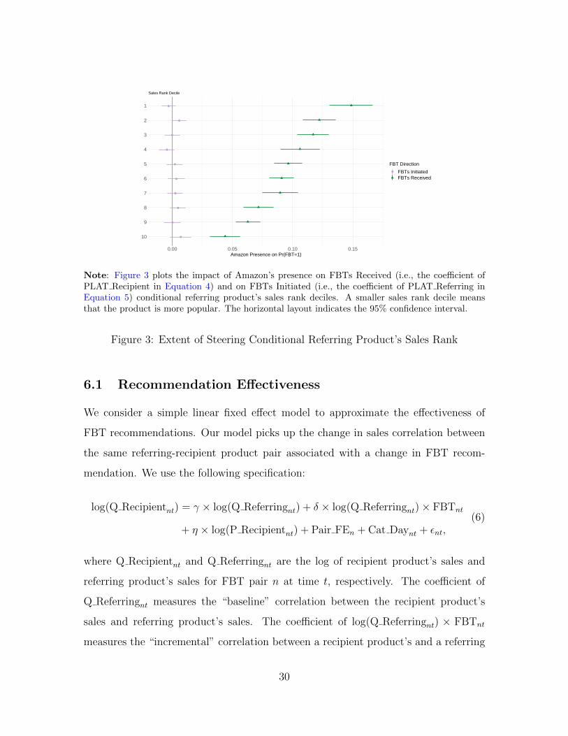
Figure 3 plot the estimates. For FBTs Received, we identify a significant extent of
steering across all the 10 sales rank deciles. When referring product is more popular,
we find a higher extent of steering. As a comparison, there is no steering for FBTs
Initiated across all the 10 deciles.
29
●
●
●
●
●
●
●
●
●
●
10
9
8
7
6
5
4
3
2
1
0.00 0.05 0.10 0.15Amazon Presence on Pr(FBT=1)
FBT Direction● FBTs Initiated
FBTs Received
Sales Rank Decile
Note: Figure 3 plots the impact of Amazon’s presence on FBTs Received (i.e., the coefficient ofPLAT Recipient in Equation 4) and on FBTs Initiated (i.e., the coefficient of PLAT Referring inEquation 5) conditional referring product’s sales rank deciles. A smaller sales rank decile meansthat the product is more popular. The horizontal layout indicates the 95% confidence interval.
Figure 3: Extent of Steering Conditional Referring Product’s Sales Rank
6.1 Recommendation Effectiveness
We consider a simple linear fixed effect model to approximate the effectiveness of
FBT recommendations. Our model picks up the change in sales correlation between
the same referring-recipient product pair associated with a change in FBT recom-
mendation. We use the following specification:
log(Q Recipientnt) = γ × log(Q Referringnt) + δ × log(Q Referringnt) × FBTnt
+ η × log(P Recipientnt) + Pair FEn + Cat Daynt + εnt,(6)
where Q Recipientnt and Q Referringnt are the log of recipient product’s sales and
referring product’s sales for FBT pair n at time t, respectively. The coefficient of
Q Referringnt measures the “baseline” correlation between the recipient product’s
sales and referring product’s sales. The coefficient of log(Q Referringnt) × FBTnt
measures the “incremental” correlation between a recipient product’s and a referring
30

product’s sale when an FBT is granted; this incremental correlation is identified
by the variation in FBT recommendation pattern within the same referring–recipient
product pair over time.22 As before, log(P Recipientnt) controls for the log of recipient
product’s market price. Pair FEn controls the fixed effects for FBT pair n. Cat Daynt
controls the category–day fixed effects for the recipient product of FBT pair n at time
t.
We use this incremental correlation as our measurement of recommendation ef-
fectiveness. The recommendation “effectiveness” may have two interpretations. The
first is how effective the FBT algorithm is in choosing a recipient product with sales
that correlate well with sales of the referring product. As suggested by its name,
“Frequently Bought Together” recommends the product that is more likely to be
bought together with the focal product by learning from non-experimental or corre-
lational consumer choice data. This interpretation does not hinge on causality. The
second interpretation of effectiveness is arguably more restrictive: what degree of in-
cremental sales the recommender system is generating. Measuring this requires us to
identify the “true” causal effect or the conversion rate of the recommender system.
While separating the two interpretations can be valuable in quantifying welfare, it
is challenging with observational data.23 In this paper, we do not distinguish these
two potential channels. This is reasonable given that our main goal is to identify
a relative (not absolute) gap in the effectiveness of FBT recommendations between
Amazon and third-party products. Regarding welfare, our results are informative
22In an alternative specification, we add FBT in Equation 6. The coefficient of FBT is small inmagnitude and not significantly different from zero. All other coefficients remain similar as in ourmain specification.
23It is well-known that the recommendation algorithm has a cold start problem and has to rely onhistorical data (Linden et al., 2003). One implication is that in a short time window, the variation inFBT recommendation patterns is more likely to be driven by historical variations in sales and onlymarginally by the current demand variations. If these are true, then within a small time window thechange in FBT recommendation is abrupt and precedes the change in sales. Plausibly, our estimatedeffect may be comparable to the causal impact of a recommendation on the recipient product’s sale.
31
if, for instance, relatively the causal and correlational parts are not systematically
correlated with Amazon’s presence.24
Table 8 reports the coefficient estimates from Equation 6. The coefficient of
log(Q Referringnt)×FBTnt indicates that the recommendation increases the correla-
tion between a recipient product’s and referring product’s sales by 0.6% on average.
We also control for the recipient product’s market price in column (2) of Table 8, the
estimates are not sensitive to this control. Consistent with Sharma et al. (2015), we
find that Amazon’s FBT recommendations have a significant and positive effect.25
Note that FBT recommendations are directional pairs. To facilitate a comparison
for FBTs Initiated, we estimate a model similar to the one in Equation 6:
log(Q Referringnt) = γ × log(Q Recipientnt) + δ × log(Q Recipientnt) × FBTnt
+ η × log(P Referringnt) + Pair FEn + Cat Daynt + εnt.(7)
Table 9 displays the regression results. This model estimates the coefficient
log(Q Referringnt) × FBTnt for initiating an FBT recommendation. The coefficient
is much smaller in magnitude and is negative. The negative sign may be explained
by potential competition between the recipient product’s and the referring product’s
respective markets. That is, a referring product may actually lose some sales when
recommending other products.
More importantly, the estimate on FBTs Initiated can serve as a reference for
evaluating the results regarding FBTs Received. Specifically, these results suggest
that our estimate of (FBTs Received) recommendation effectiveness is not mainly
driven by other unobserved factors that simultaneously determine a recommendation
link and demand correlation; otherwise, we expect to see a significant impact of FBTs
Initiated on sales in the same direction.
24For an estimation of recommendation effectiveness using observational data on Amazon, seeSharma et al. (2015). They use temporary shocks in direct traffic of the referring product whereaswe use temporary shocks in FBT recommendations.
25The absolute magnitude of our estimate does not have a direct interpretation as it is subjectto an unknown scale parameter (i.e., b in Equation 2).
32

●
●
●
●
●
●
●
●
●
●
●
●
●
●
●
●
●
●
●
●
●
●
●
●
●
●
●
●
●
●
BabyCases, Holsters & Sleeves
BeddingAccessoriesHome Decor
Fan ShopBoys
WomenHair Care
MenComputers & AccessoriesSports & Fitness Features
Skin CareSports & Fitness
Pantry StaplesOutdoor Recreation
GirlsMakeup
Kitchen & Dining FeaturesKitchen & Dining
BeveragesSubjects
TVDogs
Office & School SuppliesStyles
Health CareVitamins & Dietary Supplements
Home & Kitchen FeaturesMovies
−0.2 −0.1 0.0 0.1 0.2 0.3Amazon Presence on Pr(FBT=1)
FBT Direction
● FBTs Initiated
FBTs Received
Note: Figure 4 plots the impact of Amazon’s presence on FBTs Received (i.e., the coefficientof PLAT Recipient in Equation 4) and on FBTs Initiated (i.e., the coefficient of PLAT Referringin Equation 5) for each product category, respectively. The horizontal layout indicates the 95%confidence interval.
Figure 4: Extent of Steering across Product Categories
6.2 Heterogeneous Steering across Product Categories
Some products may have complementary products that are frequently bought to-
gether, and recommendation is more effective for more “recommendable” products.
When FBTs are more effective, steering can be more profitable. In Section 6.2, we
test the prediction that higher FBT effectiveness incentivizes more steering. We use
variations across product categories where recommendation effectiveness may differ
because of heterogeneous consumer demand patterns. For example, consumers may
be more likely to buy the recommended product for beauty products or groceries
because they usually buy multiple products at one time. Alternatively, recommenda-
tions can be more effective for TV shows or movies where consumer preference may
be more predictable. We find that Amazon steers more in product categories where
FBTs are estimated to be more effective. The pattern is consistent with Amazon’s
profit-maximizing incentive.
33

To estimate the heterogeneous steering effect, we estimate Equation 4 separately
for different product categories. We focus on the top 30 product categories to get
sufficient observations in each category. Figure 4 plots the 30 estimates on the coeffi-
cient of PLAT Recipient (in Equation 4) and PLAT Referring (in Equation 5) for all
the 30 product categories.
The value of PLAT Recipient indicates the extent of steering: conditional on price
and sales, the recipient product is more likely to receive recommendations when Ama-
zon sells the recipient product. A larger value of PLAT Recipient means that Amazon
steers more in that product category. Figure 4 shows significant heterogeneity in ex-
tent of steering across product categories. In particular, categories such as Health
Care, Vitamins & Dietary Supplements, Home & Kitchen Features, and Movies have
the strongest extent of steering. On the other hand, the value of PLAT Referring
indicates how much more likely the referring product is to initiate a recommenda-
tion when Amazon sellers the referring product. Remarkably, the estimates are not
statistically different from zero for all 30 product categories.
We then estimate recommendation effectiveness for the top 30 product categories
separately using Equation 6. Figure 5 shows the effectiveness of recommendations
(i.e., the coefficient of log Q Referringnt × FBTnt) for each product category; the fig-
ure indicates a significant difference in recommendation effectiveness across product
categories. The recommendations are particularly effective for categories such as Skin
Care, Dogs, Kitchen & Dining Features, and TV. As a useful comparison, we also
estimate and plot the coefficient of log Q Recipientnt × FBTnt for FBTs Initiated in
Equation 7. The estimated effectiveness for FBTs Initiated is more or less homoge-
neous across product categories; most values are slightly below zero.
Finally, to see whether Amazon’s steering behavior is consistent with its economic
incentives, we test whether there is a positive correlation between the estimated steer-
ing coefficient of PLAT Recipient in Equation 4 and the estimated FBT effectiveness
34

●
●
●
●
●
●
●
●
●
●
●
●
●
●
●
●
●
●
●
●
●
●
●
●
●
●
●
●
●
●
Home DecorBedding
AccessoriesMen
Cases, Holsters & SleevesComputers & Accessories
GirlsWomen
Fan ShopSports & Fitness
BoysVitamins & Dietary Supplements
Sports & Fitness FeaturesOutdoor Recreation
BabyKitchen & Dining
SubjectsPantry Staples
Health CareOffice & School Supplies
MoviesHair Care
BeveragesHome & Kitchen Features
StylesTV
DogsKitchen & Dining Features
MakeupSkin Care
−0.01 0.00 0.01 0.02 0.03FBT on Sales
FBT Direction
● FBTs Initiated
FBTs Received
Note: Figure 5 plots the recommendation effectiveness for FBTs Received (i.e., the coeffi-cient of log(Q Referring) × FBT in Equation 6) and for FBTs Initiated (i.e., the coefficient oflog(Q Recipient) × FBT in Equation 7) for each product category, respectively. The horizontallayout indicates the 95% confidence interval.
Figure 5: Recommendation Effectiveness across Product Categories
coefficient of log Q Referringnt × FBTnt in Equation 6 across product categories. We
run the following simple linear regression:
Coef PLATc = Constant + λ× Coef EFFc + εc, (8)
where Coef PLATc denotes the coefficient of PLAT Recipient in Equation 4 for cat-
egory c; Coef EFFc denotes the coefficient of PLAT Recipient in Equation 6 for cat-
egory c; Constant is the constant term in the regression.
The result is presented in Table 10; we are interested in the coefficient of Coef EFFc
in Equation 8. We find that the correlation between the extent of steering and recom-
mendation effectiveness is positive and statistically significant. Overall, our estimate
suggests that Amazon steers more where the FBTs generate more sales. Figure 6
visualizes this correlation.
35

●
●
●
●
●
●
●
●
●
●
●
●
●
●
●
●●
●
●
●
●●
●●
●
●
●
●
●
●
Accessories
Baby
Bedding
Beverages
Boys
Cases, Holsters & Sleeves
Computers & Accessories
Dogs
Fan Shop
Girls
Hair Care
Health Care
Home & Kitchen Features
Home Decor
Kitchen & DiningKitchen & Dining Features
Makeup
Men
Movies
Office & School Supplies
Outdoor Recreation
Pantry StaplesSkin Care
Sports & Fitness
Sports & Fitness Features
Styles
Subjects TV
Vitamins & Dietary Supplements
Women
−0.05
0.00
0.05
0.10
0.15
0.20
−0.005 0.000 0.005 0.010 0.015 0.020FBT Effectiveness
Ste
erin
g
Note: Figure 6 plots FBT effectiveness (x axis) and the extent of steering (y axis) by productcategories. The blue line indicates the linear fits and the gray area indicates the 95% confidenceinterval.
Figure 6: Extent of Steering and FBT Effectiveness across Product Categories
6.3 Heterogeneous Steering and Capacity Constraints
In Section 6.3, we examine the heterogeneity associated with the referring product’s
capacity constraint. By Amazon’s design, each product can have at most two slots
to recommend other products. This provides a unique opportunity to test whether
Amazon’s steering behavior depends on the number of slots utilized, as the utilization
may reflect heterogeneous recommendation effectiveness. For instance, product 1 that
used both of the slots may be an effective FBT referring product; product 2 that does
not fully use its recommendation slots may be a less effective referring product. We
conjecture that Amazon will steer more for a more effective referring product (e.g.,
product 1).
To test our conjecture, we define a product that recommends two products (i.e.,
hits the capacity constraint) for at least one round of our data collection as a capacity-
constrained product; 78.64% of the referring products are categorized as being capacity-
36

constrained under this definition. For the same referring product, variation in the
number of slots used is small in our data.
First, we run Equation 6 separately for products with and without a capacity
constraint. The results are presented in Table A.11. Consistent with our hypothesis,
the average recommendation effectiveness for a referring product without a capacity
constraint is much smaller than a capacity-constrained product. In fact, the recom-
mendation effectiveness for a referring product without a capacity constraint is not
significantly different from zero.
Second, we examine the heterogeneous extent of steering depending on capacity
constraints using Equation 4. Table A.12 shows the results. Interestingly, the extent
of steering is zero for a referring product without a capacity constraint. On the other
hand, Amazon steers more in product markets with capacity constraints. The evi-
dence suggests that our finding on the steering is consistent with Amazon’s economic
incentives.
7 Steering and FBT Efficiency
We have documented Amazon’s tendency to recommend its selling products. In this
section, we provide evidence that the steering behavior is associated with a lower
recommendation efficiency estimated using Equation 6 in Section 6.1.
A recommendation system engaging in steering may not function efficiently. To
see this, consider there are two candidate recipient products of a product recom-
mendation; Amazon may assign the recommendation to its product even when the
alternative third-party product is more effective in generating additional sales. Such
prioritization of Amazon products can conflict with true consumer preference and
lead to an inefficient allocation of recommendations. If this is the case, third-party
products can “earn” recommendations only when they can outcompete the bias. In
equilibrium, recommending third-party products may be associated with higher ef-
37
fectiveness than recommending Amazon products; Appendix C.2 provides more dis-
cussion.
Guided by this intuition, we assess heterogeneous recommendation effectiveness
depending on whether the recipient product is an Amazon product. Our analysis
below uses cross-market variations in Amazon’s presence which may not be exogenous.
To make a fair comparison, we take two steps. First, we separately estimate the cases
where the referring product is sold either by Amazon or only by a third party. By
doing so, we allow FBT effectiveness to be different depending on the types of referring
products. Second, to obtain more balanced samples, we conduct a propensity score
matching for recipient products sold by Amazon and third-party sellers, respectively.
Specifically, we first focus on the pairs that experience variations in recommen-
dation patterns over the five rounds of data collection. We then divide the pairs by
product category and by whether Amazon sells in the referring product’s market. We
have 30 product categories and 2 referring product types, so there are 30 × 2 = 60
combinations in total. Within each product category and each referring product type
(Amazon or third-party referring products), we match the first round’s market char-
acteristics such as sales and seller density to form two balanced samples– a treatment
sample for Amazon recipient products and a control sample for third-party recipient
products. The matched samples are summarized in Table A.13.
Using the matched sample, we estimate the heterogeneous recommendation effec-
tiveness depending on whether Amazon sells in the recipient’s market. We run the
following:
log(Q Recipientnt) =∑k=0,1
(γk × log(Q Referringnt) + δk × log(Q Referringnt) × FBTnt)
× (1(PLAT Recipientnt = k)) + η × log(P Recipientnt)
+ Pair FEn + Cat Dayt + εnt.
(9)
38

We estimate Equation 9 separately for the case when the referring product is
an Amazon product and the case when the referring product is a third-party prod-
uct. Table 11 reports the heterogeneous recommendation effectiveness. The case of
an Amazon referring product is in columns (1) and (2). The case of a third-party
referring product is in columns (3) and (4). Within each of the four columns, the
recommendation effectiveness for Amazon recipient products is consistently smaller
than the recommendation effectiveness for third-party recipient products. When re-
ferring product is sold by a third-party, recommending third-party recipient products
is about 50% more effective than recommending one of Amazon recipient products
(e.g., 1.2% versus 0.8%). When the referring product is sold by Amazon, recommend-
ing third-party recipient products is nearly 85% more effective than recommending
Amazon recipient products (e.g., 1.5% versus 0.8%).
If Amazon does not prioritize products based on whether itself is a seller but
makes recommendations purely based on product complementarity, we expect the
estimates to be insensitive to the types of the recipient product. For contrast, we
conduct a similar matching procedure and estimation as in Equation 9 for FBTs
Initiated. Table 12 presents the results. As opposed to FBTs Received, the coefficient
of recommendation effectiveness is very similar regardless of whether Amazon sells in
the recipient market.
Moreover, we estimate recommendation effectiveness by conditioning on not only
Amazon’s presence but also capacity constraints, as in Section 6.3. We follow a sim-
ilar matching procedure to facilitate the comparisons. The estimation results are
presented in Table A.14. Third-party recipient products have higher average rec-
ommendation effectiveness than Amazon recipient products. The difference in rec-
ommendation effectiveness is robust across all referring product types. Interestingly,
when the referring product’s recommendation slots are not fully utilized, the effec-
tiveness of recommending Amazon products is not statistically greater than zero. In
39

Appendix F, we examine heterogeneous recommendation efficiency across product
categories.
We show that the FBT recommendation system does not act in the most efficient
way and maximize total sales. The results further imply that the steering poten-
tially hurts consumers and third-party sellers; consumers are directed towards a less
preferred product and third-party sellers’ offers benefit less due to the algorithmic
steering. If Amazon and third-party sellers have similar costs, the steering could lead
to deadweight loss.
8 Conclusion
Digital technologies are giving platform owners unprecedented power in today’s econ-
omy. Concerns over the (mis)use of data and algorithm may be particularly height-
ened for dual-role platforms that are both intermediaries and sellers. Empirical re-
search is limited by the lack of appropriate data as well as the ability to establish
causality.
We provide novel evidence that a platform’s dual role may affect algorithmic
recommendations. We use a unique research design and unique high-frequency data
for over 6.7 million products sold on Amazon. We show that Amazon products receive
substantially more FBT recommendations than third-party products. The pattern
is remarkably consistent across popularity deciles and product categories. Causal
analysis shows that Amazon is steering customers towards Amazon products; whether
Amazon is a seller affects FBT recommendations. A number of falsification tests
suggest that the steering is driven by seller identities instead of consumer demand.
Finally, the steering potentially hurts consumers and third-party sellers.
The paper contributes to the discussion on algorithmic recommendations in par-
ticular and competition policy and algorithmic accountability in general. Algorithmic
recommendation based on big data and machine learning is expected to be increas-
40

ingly prevalent, and will have consequences in terms of social welfare. For instance,
AI-powered digital assistants such as Amazon Alexa may take algorithmic recommen-
dations to the next level.26 Our evidence suggests that market structure can impact
the behavior of algorithms. Biases in algorithmic recommendations can be costly to
detect and correct, leading to multi-front institutional and technological challenges
(e.g., Cremer et al., 2019, Scott Morton et al., 2019, and Cowgill and Tucker, 2020).
These questions are of utmost importance, and should be studied by researchers.
References
Aguiar, L. and Waldfogel, J. (2018). Platforms, Promotion, and Product Discovery:
Evidence from Spotify Playlists. Technical report, National Bureau of Economic
Research.
Asker, J. (2016). Diagnosing Foreclosure Due to Exclusive Dealing. The Journal of
Industrial Economics, 64(3):375–410.
Atalay, E., Hortacsu, A., and Syverson, C. (2014). Vertical Integration and Input
Flows. American Economic Review, 104(4):1120–48.
Barwick, P. J., Pathak, P. A., and Wong, M. (2017). Conflicts of Interest and Steer-
ing in Residential Brokerage. American Economic Journal: Applied Economics,
9(3):191–222.
Bergemann, D. and Bonatti, A. (2019). The Economics of Social Data: An Introduc-
tion.
Bergemann, D., Bonatti, A., and Gan, T. (2019). The Economics of Social Data.
Manuscript.
Berto Villas-Boas, S. (2007). Vertical Relationships Between Manufacturers and Re-
tailers: Inference With Limited Data. The Review of Economic Studies, 74(2):625–
652.
26See page 310-312 in https://judiciary.house.gov/uploadedfiles/competition_in_
digital_markets.pdf.
41

Bezos, J. (1997). Amazon 1997 Letter to Shareholders.
Bezos, J. (2005). Amazon 2005 Letter to Shareholders.
Bezos, J. (2017). Amazon 2017 Letter to Shareholders.
Bezos, J. (2018). Amazon 2018 Letter to Shareholders.
Brot-Goldberg, Z. C. and de Vaan, M. (2018). Intermediation and Vertical Integration
in the Market for Surgeons. Technical report.
Burguet, R., Caminal, R., and Ellman, M. (2015). In Google We Trust? International
Journal of Industrial Organization, 39:44–55.
Bushnell, J. B., Mansur, E. T., and Saravia, C. (2008). Vertical Arrangements,
Market Structure, and Competition: An Analysis of Restructured US Electricity
Markets. American Economic Review, 98(1):237–66.
Chevalier, J. and Goolsbee, A. (2003). Measuring Prices and Price Competition
Online: Amazon.com and Barnesandnoble.com. Quantitative Marketing and Eco-
nomics, 1(2):203–222.
Chevalier, J. A. and Mayzlin, D. (2006). The Effect of Word of Mouth on Sales:
Online Book Reviews. Journal of Marketing Research, 43(3):345–354.
Chipty, T. (2001). Vertical Integration, Market Foreclosure, and Consumer Welfare
in the Cable Television Industry. American Economic Review, 91(3):428–453.
Cowgill, B. and Tucker, C. E. (2020). Algorithmic Fairness and Economics. The
Journal of Economic Perspectives.
Crawford, G. S., Lee, R. S., Whinston, M. D., and Yurukoglu, A. (2018). The Welfare
Effects of Vertical Integration in Multichannel Television Markets. Econometrica,
86(3):891–954.
Cremer, J., de Montjoye, Y.-A., and Schweitzer, H. (2019). Competition Policy for
the Digital Era. Technical report, European Commission.
De Corniere, A. and Taylor, G. (2014). Integration and Search Engine Bias. The
RAND Journal of Economics, 45(3):576–597.
42

De Corniere, A. and Taylor, G. (2019). A Model of Biased Intermediation. The
RAND Journal of Economics.
Dinerstein, M., Einav, L., Levin, J., and Sundaresan, N. (2018). Consumer Price
Search and Platform Design in Internet Commerce. American Economic Review,
108(7):1820–59.
Edelman, B. (2011). Bias in Search Results: Diagnosis and Response. Indian JL
Tech., 7:16.
EU Commission (2020). Antitrust: Commission sends statement of objections to
amazon for the use of non-public independent seller data and opens second inves-
tigation into its e-commerce business practices.
Gomez-Uribe, C. A. and Hunt, N. (2016). The Netflix Recommender System: Al-
gorithms, Business Value, and Innovation. ACM Transactions on Management
Information Systems (TMIS), 6(4):13.
Hagiu, A. and Jullien, B. (2011). Why Do Intermediaries Divert Search? The RAND
Journal of Economics, 42(2):337–362.
Hastings, J. S. and Gilbert, R. J. (2005). Market Power, Vertical Integration and the
Wholesale Price of Gasoline. The Journal of Industrial Economics, 53(4):469–492.
Hortacsu, A. and Syverson, C. (2007). Cementing Relationships: Vertical Integration,
Foreclosure, Productivity, and Prices. Journal of political economy, 115(2):250–301.
Houde, J.-F. (2012). Spatial Differentiation and Vertical Mergers in Retail Markets
for Gasoline. American Economic Review, 102(5):2147–82.
Khan, L. M. (2016). Amazon’s Antitrust Paradox. Yale LJ, 126:710.
Lee, R. S. (2013). Vertical Integration and Exclusivity in Platform and Two-Sided
Markets. American Economic Review, 103(7):2960–3000.
Linden, G., Smith, B., and York, J. (2003). Amazon. Com Recommendations: Item-
To-Item Collaborative Filtering. IEEE Internet Computing, pages 76–80.
Luco, F. and Marshall, G. (2020). The Competitive Impact of Vertical Integration
by Multiproduct Firms. American Economic Review, 110(7):2041–64.
43
McManus, B., Nevo, A., Nolan, Z., and Williams, J. W. (2020). Steering incentives
of platforms: Evidence from the telecommunications industry. Technical report,
National Bureau of Economic Research.
Mullainathan, S. and Obermeyer, Z. (2017). Does Machine Learning Automate Moral
Hazard and Error? American Economic Review, 107(5):476–80.
Obermeyer, Z., Powers, B., Vogeli, C., and Mullainathan, S. (2019). Dissecting
Racial Bias in an Algorithm Used to Manage the Health of Populations. Science,
366(6464):447–453.
Rambachan, A., Kleinberg, J., Ludwig, J., and Mullainathan, S. (2020). An Economic
Perspective on Algorithmic Fairness. In AEA Papers and Proceedings, volume 110,
pages 91–95.
Scott Morton, F., Bouvier, P., Ezrachi, A., Jullien, B., Katz, R., Kimmelman, G.,
Melamed, A. D., and Morgenstern, J. (2019). Committee for the Study of Digital
Platforms: Market Structure and Antitrust Subcommittee Report. Draft.
Sharma, A., Hofman, J. M., and Watts, D. J. (2015). Estimating the Causal Impact of
Recommendation Systems from Observational Data. In Proceedings of the Sixteenth
ACM Conference on Economics and Computation, pages 453–470. ACM.
Smith, B. and Linden, G. (2017). Two Decades of Recommender Systems at Ama-
zon.com. IEEE Internet Computing, 21(3):12–18.
Teh, T.-H. and Wright, J. (2020). Intermediation and Steering: Competition in Prices
and Commissions. American Economic Journal: Microeconomics.
Waterman, D. and Weiss, A. A. (1996). The Effects of Vertical Integration Between
Cable Television Systems and Pay Cable Networks. Journal of Econometrics, 72(1-
2):357–395.
Zhu, F. and Liu, Q. (2018). Competing with Complementors: An Empirical Look at
Amazon.com. Strategic Management Journal, 39(10):2618–2642.
44

Table 1: Summary of Market Structure
Percentage Count
Panel A: All ProductsAmazon Only 4.2% 286,355Amazon and Third-Party 14.5% 981,771Third-Party Only 81.3% 5,498,652
Total 100% 6,766,778
Panel B: Products with RecommendationsAmazon Only 3.4% 138,775Amazon and Third-Party 19.1% 788,511Third-Party Only 77.6% 3,206,765
Total 100% 4,134,051
Note: Table 1 shows the summary of market structure. Panel A shows the full sample. Panel Bshows the summary statistics of the products that receive or initiate at least one recommendationin our data. The unit of observation is at the product level.
Table 2: Summary of Product Characteristics
Mean Standard Deviation Minimum Maximum
Panel A: All ProductsMarket Price 40.54 99.19 0.00 50,947.65Sales Rank 931,807.01 2,612,298.90 1.00 28,894,712.00Number of Sellers 3.02 9.63 1.00 5,872.00Number of FBTs Received 0.68 10.00 0.00 11,012.00Number of FBTs Initiated 0.91 0.85 0.00 2.00
No. of Observations 6,766,778
Panel B: Products with RecommendationsMarket Price 34.00 75.04 0.01 32,039.35Sales Rank 548,296.37 1,824,082.91 1.00 28,780,820.00Number of Sellers 3.44 7.41 1.00 5,872.00Number of FBTs Received 1.12 12.78 0.00 11012.00Number of FBTs Initiated 1.49 0.56 0.00 2.00
No. of Observations 4,134,051
Note: Table 2 shows the summary statistics of the products in our data. Panel A shows the fullsample. Panel B shows the summary statistics of the products that receive or initiate at least onerecommendation in our data.
45
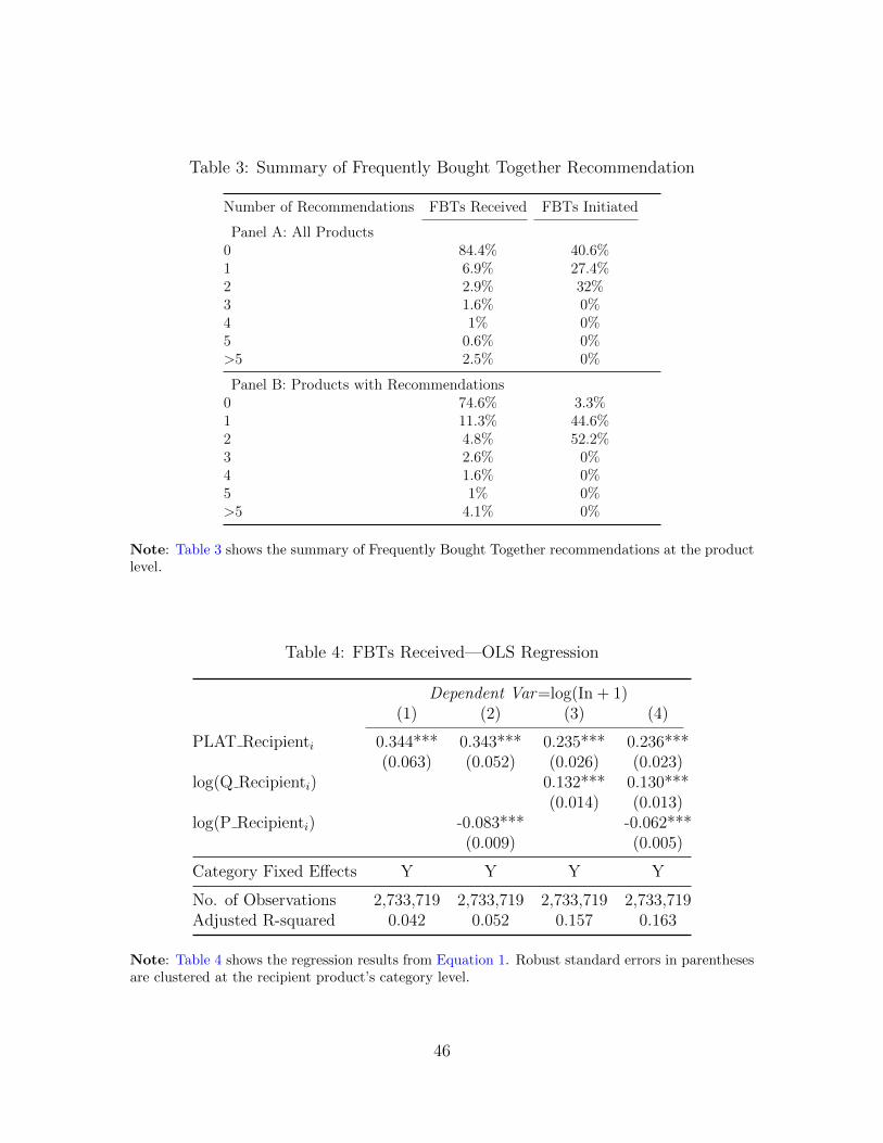
Table 3: Summary of Frequently Bought Together Recommendation
Number of Recommendations FBTs Received FBTs Initiated
Panel A: All Products0 84.4% 40.6%1 6.9% 27.4%2 2.9% 32%3 1.6% 0%4 1% 0%5 0.6% 0%>5 2.5% 0%
Panel B: Products with Recommendations0 74.6% 3.3%1 11.3% 44.6%2 4.8% 52.2%3 2.6% 0%4 1.6% 0%5 1% 0%>5 4.1% 0%
Note: Table 3 shows the summary of Frequently Bought Together recommendations at the productlevel.
Table 4: FBTs Received—OLS Regression
Dependent Var=log(In + 1)(1) (2) (3) (4)
PLAT Recipienti 0.344*** 0.343*** 0.235*** 0.236***(0.063) (0.052) (0.026) (0.023)
log(Q Recipienti) 0.132*** 0.130***(0.014) (0.013)
log(P Recipienti) -0.083*** -0.062***(0.009) (0.005)
Category Fixed Effects Y Y Y Y
No. of Observations 2,733,719 2,733,719 2,733,719 2,733,719Adjusted R-squared 0.042 0.052 0.157 0.163
Note: Table 4 shows the regression results from Equation 1. Robust standard errors in parenthesesare clustered at the recipient product’s category level.
46

Table 5: Variations in FBTs Received Depending on Amazon’s Presence
Dependent Var=FBTt
(1) (2) (3)
PLAT Recipientt 0.087*** 0.083*** 0.080***(0.016) (0.015) (0.014)
log(Q Recipientt) 0.016*** 0.016***(0.003) (0.003)
log(P Recipientt) -0.014***(0.004)
Product Pair Fixed Effects Y Y YCategory–Day Fixed Effects Y Y Y
No. of Observations 32,375,268 32,375,268 32,375,268Adjusted R-squared 0.397 0.397 0.397
Note: Table 5 reports coefficient estimates of interest from Equation 4. The dependent variable is anindicator of whether the referring product recommends the recipient product in a pair. Other coeffi-cients and fixed effects are omitted for brevity. Robust standard errors in parentheses are clusteredat the recipient product’s category level. Significance levels: *(p<0.10), **(p<0.05), ***(p<0.01).
Table 6: Variations in FBTs Initiated Depending on Amazon’s Presence
Dependent Var=FBTt
(1) (2) (3)
PLAT Referringt 0.001** 0.001*** 0.001*(0.000) (0.000) (0.001)
log(Q Referringt) -0.002*** -0.002***(0.000) (0.001)
log(P Referringt) -0.002(0.003)
Product Pair Fixed Effects Y Y YCategory–Day Fixed Effects Y Y Y
No. of Observations 29,819,329 29,819,329 29,819,329Adjusted R-squared 0.360 0.360 0.360
Note: Table 6 reports coefficient estimates of interest from Equation 5. The dependent variable is anindicator of whether the referring product recommends the recipient product in a pair. Other coeffi-cients and fixed effects are omitted for brevity. Robust standard errors in parentheses are clusteredat the recipient product’s category level. Significance levels: *(p<0.10), **(p<0.05), ***(p<0.01).
47

Table 7: Effect of Amazon’s Presence and Seller Identities on Recommendations
Dependent Var=FBTt
(1) (2) (3) (4) (5) (6)
FBA Sellers FBM Sellers
PLAT Recipientt 0.071*** 0.068*** 0.065*** 0.092*** 0.087*** 0.084***(0.016) (0.015) (0.015) (0.02) (0.017) (0.017)
log(Q Recipientt) 0.015*** 0.015*** 0.017*** 0.016***(0.003) (0.003) (0.005) (0.005)
log(P Recipientt) -0.014*** -0.015***(0.004) (0.005)
Product Pair Fixed Effects Y Y Y Y Y YCategory–Day Fixed Effects Y Y Y Y Y Y
No. of Observations 13,551,634 13,551,634 13,551,634 4,061,672 4,061,672 4,061,672Adjusted R-squared 0.464 0.464 0.464 0.472 0.472 0.472
Note: Table 7 reports coefficient estimates of interest from Equation 4 separately for recipient prod-ucts that have at least one FBA seller or have no FBA seller. The dependent variable is an indicatorof whether the referring product recommends the recipient product in a pair. Other coefficientsand fixed effects are omitted for brevity. Robust standard errors in parentheses are clustered at therecipient product’s category level. Significance levels: *(p<0.10), **(p<0.05), ***(p<0.01).
Table 8: Effectiveness of FBTs Received
Dependent Var=log(Q Recipientt)(1) (2)
log(Q Referringt) 0.345*** 0.346***(0.003) (0.033)
log(Q Referringt)×FBTt 0.006*** 0.006***(0.000) (0.001)
log(P Recipientt) -0.224***(0.078)
Product Pair Fixed Effects Y YCategory–Day Fixed Effects Y Y
No. of Observations 30,539,061 30,539,061Adjusted R-squared 0.960 0.960
Note: Table 8 reports coefficient estimates of interest from Equation 6 using the recipient product’ssales as the outcome variable. Other coefficients and fixed effects are omitted for brevity. Robuststandard errors in parentheses are clustered at the recipient product’s category level. Significancelevels: *(p<0.10), **(p<0.05), ***(p<0.01).
48

Table 9: Effectiveness of FBTs Initiated
Dependent Var=log(Q Referringt)(1) (2)
log(Q Recipientt) 0.288*** 0.288***(0.044) (0.044)
log(Q Recipientt)×FBTt -0.002*** -0.002***(0.000) (0.000)
log(P Referringt) -0.151*(0.082)
Product Pair Fixed Effects Y YCategory–Day Fixed Effects Y Y
No. of Observations 26,861,632 26,861,632Adjusted R-squared 0.962 0.962
Note: Table 9 reports coefficient estimates of interest from Equation 7 using referring product’ssales as the outcome variable. Other coefficients and fixed effects are omitted for brevity. Robuststandard errors in parentheses are clustered at the referring product’s category level. Significancelevels: *(p<0.10), **(p<0.05), ***(p<0.01).
Table 10: Correlation across Product Categories
Dependent Var=Coef PLATc
(1)
Coef EFFc 6.020***(1.757)
Constant 0.028(0.017)
No. of Observations 30Adjusted R-squared 0.270
Note: Table 10 shows the coefficients in Equation 8. The dependent variable is the extent of steering(i.e., the coefficient of PLAT Recipient in Equation 4). Robust standard errors in parentheses.Significance levels: *(p<0.10), **(p<0.05), ***(p<0.01).
49

Table 11: Matched Sample: Effectiveness of FBTs Received Depending on Amazon’sPresence
Dependent Var=log(Q Recipientt)(1) (2) (3) (4)
PLAT Referringt = 0 PLAT Referringt = 1
FBTt × 1(PLAT Recipientt = 0) × log(Q Referringt) 0.012*** 0.012*** 0.015*** 0.015***(0.004) (0.004) (0.005) (0.005)
FBTt × 1(PLAT Recipientt = 1) × log(Q Referringt) 0.008*** 0.008*** 0.008*** 0.008***(0.001) (0.001) (0.001) (0.002)
1(PLAT Recipientt = 0) × log(Q Referringt) 0.377*** 0.379*** 0.329*** 0.334***(0.054) (0.053) (0.023) (0.023)
1(PLAT Recipientt = 1) × log(Q Referringt) 0.364*** 0.363*** 0.335*** 0.334***(0.031) (0.032) (0.021) (0.021)
log(P Recipientt) -0.083 -0.256*(0.110) (0.139)
Product Pair Fixed Effects Y Y Y YCategory–Day Fixed Effects Y Y Y Y
No. of Observations 2,207,567 2,207,567 2,389,118 2,389,118Adjusted R-squared 0.946 0.946 0.951 0.952
Note: Table 11 reports coefficient estimates of interest in Equation 9 using recipient product’s salesas the outcome variable in the matched sample. Other coefficients and fixed effects are omittedfor brevity. Robust standard errors in parentheses are clustered at the recipient product’s categorylevel. Significance levels: *(p<0.10), **(p<0.05), ***(p<0.01).
Table 12: Matched Sample: Effectiveness of FBTs Initiated Depending on Amazon’sPresence
Dependent Var=log(Q Referringt)(1) (2) (3) (4)
PLAT Recipient= 0 PLAT Recipientt = 1
FBTt × 1(PLAT Referringt = 0) × log(Q Recipientt) -0.002*** -0.002*** -0.002*** -0.002***(0.000) (0.000) (0.000) (0.000)
FBTt × 1(PLAT Referringt = 1) × log(Q Recipientt) -0.002** -0.002** -0.002*** -0.002***(0.001) (0.001) (0.000) (0.000)
1(PLAT Referringt = 0) × log(Q Recipientt) 0.323*** 0.324*** 0.243*** 0.244***(0.023) (0.023) (0.015) (0.015)
1(PLAT Referringt = 1) × log(Q Recipientt) 0.326*** 0.325*** 0.256*** 0.254***(0.021) (0.020) (0.014) (0.014)
log(P Referringt) -0.220*** -0.143*(0.058) (0.078)
Product Pair Fixed Effects Y Y Y YCategory–Day Fixed Effects Y Y Y Y
No. of Observations 597,433 597,433 2,477,805 2,477,805Adjusted R-squared 0.940 0.940 0.958 0.958
Note: Table 12 reports coefficient estimates of interest in Equation 9 using referring product’s salesas the outcome variable in the matched sample. Other coefficients and fixed effects are omittedfor brevity. Robust standard errors in parentheses are clustered at the referring product’s categorylevel. Significance levels: *(p<0.10), **(p<0.05), ***(p<0.01).
50

Online Appendix (Not Intended for Publication)
A Cross-Product Regressions For Amazon-Only Mar-
kets
In Section 4.1, we conduct cross-product regressions where Amazon markets include
both markets with only Amazon and markets with both Amazon and third-party
sellers. Here we conduct cross-product analysis and focus on the markets where
Amazon is the only seller.27 We exclude the markets with both Amazon and third-
party sellers and use the markets with only third-party sellers as the comparison
group. Table A.2 presents the results for FBTs Received using Equation 1. Table A.3
presents the results for FBTs Initiated using Equation 3. The results are qualitatively
similar to Section 4.1.
B Event Study
To understand the trends of sales and prices the variation in Amazon’s presence, we
employ the following empirical design:
Yit =5∑
k=−5,k 6=−1
πk×Dkit+
(5∑
k=−5,k 6=−1
ρk ×Dkit
)×Treati+Prod FEi+Cat Dayit+ εit,
(A.1)
where Yit is the outcome variable for event i at day t. Dkit = I
{t = eventit + 3k
}is an indicator of whether Amazon entered or exited the marketplace 3k days ago
and eventit denotes the day of event i (Amazon entered or exited) at day t. We
denote Treat as an indicator of whether the event is a member of the treatment group
27Products where Amazon is the sole seller (e.g., Amazon private-label products) areless significant. The sales of private-brand products represent only 1% of Amazon’s first-party sales. See page 24 in https://docs.house.gov/meetings/JU/JU05/20200729/110883/
HHRG-116-JU05-20200729-QFR052.pdf.
1

(Treat = 1) or the control group (Treat = 0); We construct the control group in the
following way: we randomly draw placebo event dates from the empirical distribution
of real event dates using the same set of products. That is, the control group consists
of the same set of products as the treatment group, but the events are fictitious.
We include product fixed effects Prod FEi to control for variations that differ across
products but are constant over time. We also include product category–day fixed
effects Cat Dayit to control for product-category-specific time trends. The standard
errors are clustered on both product and monthly levels.
The specification is to compare the sales for the treatment group relative to the
control group before and after an event.28
Figure A.8(a) and Figure A.8(c) plot the coefficients from Equation A.1 using
the log of sales as the outcome variable for Amazon’s entry and exit, respectively.
Similarly, we approximate the log of sales using a linear function of the log of sales
ranks as in Equation 2. Figure A.8(b) and Figure A.8(d) plot the coefficients from
Equation A.1 using the log of market prices as the outcome variable for Amazon’s
entry and exit, respectively. The pre-trends of sales and price are relatively smooth
and the discontinuities are sharp, suggesting that variation in Amazon’s presence is
plausibly exogenous. Note that there are around 9% change in prices and 15% change
in sales after Amazon’s entry or exit. The signs of the changes are expected. These
changes cannot explain our result on steering. First, we control for real-time prices
and sales in our main model and find that both have little impact on our result.
Second, we show that after manually adding even 100% changes to prices and sales,
our results are still robust.
28The specification is similar to difference-in-differences, but the post indicator is replaced by thenumber of days since the event, and treati is absorbed by event fixed effects Evnt FE.
2

Referring Product
Recipient Product iRecipient Product j
ck + εirkck + εjrk
Note: Figure A.1 illustrates the directionality for a product recommendation.
Figure A.1: Directionality of A Product Recommendation
C Model of Steering
We develop a toy model of steering using product recommendations for a profit-
maximizing platform. The model predicts that the likelihood of receiving a recom-
mendation increases when Amazon sells the product.
Figure A.1 illustrates the directionality of a product recommendation. For a given
referring product r, Amazon has one slot to display the recommending product and
is choosing between two products in the category k, an Amazon product i and a
third-party product j; that is, Amazon’s share for product i is greater than 0 and for
product j is 0 (i.e., si ≥ 0, and sj = 0); cirk denotes the conversion rate, which means
that referring a recommendation to product i leads to sales of cirk ×Qr , where Qr is
the sales of the referring product r.
A product i’s conversion rate cirk of category k follows
cirk = ck + εirk,
where ε is distributed independent and identically distributed across products with
mean zeros and support [l, u].
3

C.1 Recommendation Choices
Amazon’s profit for recommending product i and product j follows
Π(Recomr = i) = (πi × si + Fee × (1 − si)) × (ck + εirk) ×Qr,
Π(Recomr = j) = Fee × (ck + εjrk) ×Qr,
where πi is Amazon’s retail margin for selling the product i. When Amazon sells the
product, it earns the retail margin. Fee is the average referral fee (or commission
fee) paid by third-party sellers when they sell the product. Naturally, we assume the
condition that πi > Fee; Amazon’s retail margin is higher than the referral fee when
it chooses to sell.
Amazon would choose to recommend the product that would draw a greater profit
for itself. The probability of recommending its product i from referring product r is
Pr(Recomr = i) = Pr(Π(Recomr = i) > Π(Recomr = j))
= Pr
[πi
Fee× si + (1 − si)︸ ︷︷ ︸≡ηik≥1
] × (ck + εirk) − (ck + εjrk) > 0
,
= Pr(ηikεirk − εjrk > (1 − ηik)︸ ︷︷ ︸≤0
×ck).
(A.2)
According to Equation A.2, product i’s probability of receiving a recommendation
from referring product r increases when Amazon sells the product (i.e., when si > 0);
this prediction is consistent with our empirical finding in Section 5.
Moreover, product i’s probability of receiving a recommendation increases when
the recommendation in its category is more effective on average (i.e., a larger c); this
prediction is consistent with the empirical finding in Section 6.2.
4
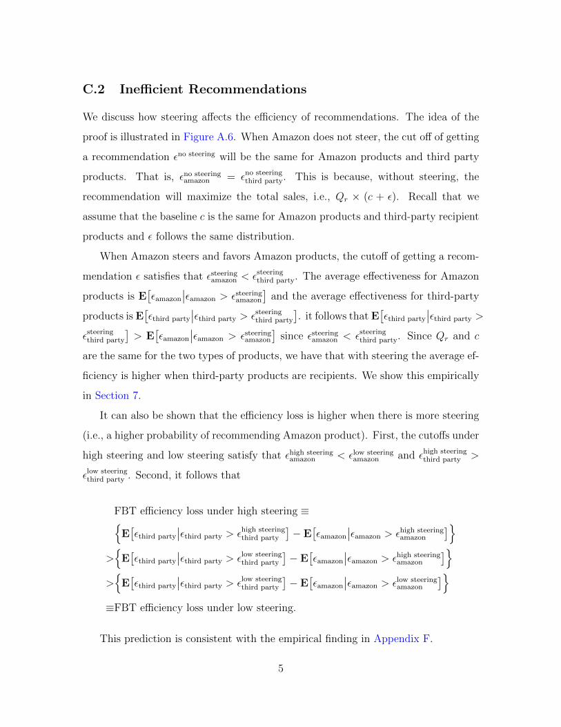
C.2 Inefficient Recommendations
We discuss how steering affects the efficiency of recommendations. The idea of the
proof is illustrated in Figure A.6. When Amazon does not steer, the cut off of getting
a recommendation εno steering will be the same for Amazon products and third party
products. That is, εno steeringamazon = εno steering
third party. This is because, without steering, the
recommendation will maximize the total sales, i.e., Qr × (c + ε). Recall that we
assume that the baseline c is the same for Amazon products and third-party recipient
products and ε follows the same distribution.
When Amazon steers and favors Amazon products, the cutoff of getting a recom-
mendation ε satisfies that εsteeringamazon < εsteeringthird party. The average effectiveness for Amazon
products is E[εamazon
∣∣εamazon > εsteeringamazon
]and the average effectiveness for third-party
products is E[εthird party
∣∣εthird party > εsteeringthird party
]. it follows that E
[εthird party
∣∣εthird party >
εsteeringthird party
]> E
[εamazon
∣∣εamazon > εsteeringamazon
]since εsteeringamazon < εsteeringthird party. Since Qr and c
are the same for the two types of products, we have that with steering the average ef-
ficiency is higher when third-party products are recipients. We show this empirically
in Section 7.
It can also be shown that the efficiency loss is higher when there is more steering
(i.e., a higher probability of recommending Amazon product). First, the cutoffs under
high steering and low steering satisfy that εhigh steeringamazon < εlow steering
amazon and εhigh steeringthird party >
εlow steeringthird party . Second, it follows that
FBT efficiency loss under high steering ≡{E[εthird party
∣∣εthird party > εhigh steeringthird party
]− E
[εamazon
∣∣εamazon > εhigh steeringamazon
]}>{
E[εthird party
∣∣εthird party > εlow steeringthird party
]− E
[εamazon
∣∣εamazon > εhigh steeringamazon
]}>{
E[εthird party
∣∣εthird party > εlow steeringthird party
]− E
[εamazon
∣∣εamazon > εlow steeringamazon
]}≡FBT efficiency loss under low steering.
This prediction is consistent with the empirical finding in Appendix F.
5

D Robustness Checks: Tendency to Recommend
Amazon Products
We perform several robustness checks. We show that our results of steering are robust
under alternative models such as probit and logit instead of linear probability models.
We test that including lagged sales and prices does not affect our estimates. Lastly,
we use placebo Amazon presence for falsification tests.
D.1 Probit and Logistic Regression
We examine Equation 4 using probit regression and logistic regression. Column (2) of
Table A.4 shows the results from logistic regression; Column (3) of Table A.4 shows
the results from probit regression. The marginal effects of Amazon’s presence are
comparable to our main results using a linear model.
D.2 Controlling for Lagged Sales and Prices
In Table A.5, we control for lagged sales and prices in Equation 4. We add sales and
prices in 5-day, 10-day, and 15-day lag. The effects of Amazon’s presence on FBTs
Received are fairly similar across columns. The estimated effect is not sensitive to
these controls.
D.3 Placebo Amazon’s Presence
To highlight our source of identification, within a pair of products, we randomize
Amazon’s presence within products across rounds. We then examine Equation 4
replacing Amazon’s presence with the placebo Amazon’s presence.
We display the results using placebo Amazon’s presence in Table A.6. The effect of
placebo Amazon’s presence on FBTs Received is small and statistically insignificant.
6

E Supporting Results
We present additional results below. Our goal is to show that the steering behavior
cannot be explained by consumer demand.
E.1 Price Perturbation
Figure A.7 plots the distribution of shipping costs for FBM offers. 53.9% of FBM
offers do not charge for shipping. 28.6% of FBM offers charge $3.99 for shipping.
To make sure that our results are not driven by shipping cost or other measure-
ment errors in prices, we manually increase the market price after Amazon experiences
a stock out in Equation 4. This helps to explain that whether the steering is driven
by price rather than by Amazon’s temporary absence directly. Table A.7 shows re-
sults. From columns (1)–(3), we add $3.99, $11.85 and $37.87 respectively. Over
60% ≈ 28.6%1−53.9% FBM offers charge $3.99 when they charge any shipping cost. $11.85
and $37.87 correspond to the 99% and 99.9% percentile of the shipping cost. Over-
all, our estimate is not significantly affected. This also suggests that the price-based
explanation cannot explain the steering as the average product price is only $34 (see
Panel B in Table 2) and column (3) implies over 100% measurement error in prices.
E.2 Sales Perturbation
To check that our results are not sensitive to any measurement errors of sales, we
also perturb recipient products’ sales in Equation 4. In Table A.8, we increase the
sales before Amazon experiences a stock out by 10%, 30%, and 100%, respectively.
The effects of Amazon’s presence on FBTs Received are all significant under these
different levels of perturbation.
7

E.3 Effect of Third-Party Seller’s Presence
To check that our results in Section 5 are not driven by the unobservables that are
correlated with sellers’ presence, we check whether the probability of receiving an
FBT recommendation depends on a third-party seller’s presence. We replace the
indicator of Amazon’s presence with the indicator of a third-party seller’s presence in
Equation 4 as the following:
FBTnt = κ× 3Party Recipientnt + γ × log(Q Recipientnt)
+ η × log(P Recipientnt) + Pair FEn + Cat Daynt + εnt,(A.3)
where 3Party Recipientnt indicates whether a third-party seller enters the recipient
product’s market in pair n at time t.
Table A.9 displays the results from Equation A.3. The coefficient of a third-
party’s presence is not statistically different from 0 (i.e., about 27 times smaller than
the coefficient of Amazon’s presence in Table 5); the probability of receiving an FBT
recommendation does not depend on a third-party seller’s presence.
Table A.10 displays the results from Equation 5 when we replace the indicator
of Amazon’s presence with the indicator of a third-party seller’s presence. Similar
to our finding for Amazon’s presence in Table 6, the effect of a third-party seller’s
presence on FBTs Initiated is small in all specifications.
F Extent of Steering and Loss of FBT Efficiency
across Product Categories
Section 6.2 shows cross-category variations in the extent of steering. As predicted
by Amazon’s economic incentives, the variations in the extent of steering can be
explained by variations in recommendation effectiveness. In this section, we test if
8

the cross-category variations in the loss of FBT efficiency can be explained by the
cross-category variations in the extent of steering estimated in Section 6.2.
As in Section 7, for each product category, we match market characteristics such
as sales and seller density to form two balanced samples of recipient products—one of
Amazon products and one of third-party products. We use the matched samples to
estimate the heterogeneous recommendation effects depending on Amazon’s presence
in the recipient market for all 30 product categories. For each product category, we
define the loss of FBT efficiency as the difference in effectiveness estimates between
recommending third-party product and recommending Amazon product. We run the
following linear regression:
Coef Lossc = Constant + λ× Coef PLATc + εc, (A.4)
where Coef Lossc denotes efficiency loss for category c.
Table A.15 presents the regression results. Consistent with our hypothesis, we
find a significant positive correlation between the extent of steering and the loss of
FBT efficiency across product categories. Figure A.9 visualizes this correlation.
9

(a) Cross-Product Variation
(b) Within-Product Variation from Amazon Stockout
Figure A.2: Summary of Identification
Note: Figure A.2(a) summaries our cross-product comparisons. Figure A.2(b) summaries our mainresearch design using within-product variation from Amazon stockouts.
10

●
●
●
●
●
●
●
●
●
●
●
●
●
●
●
●
●
●
●
●
●
●
●
●
●
●
●
●
●
●
Cases, Holsters & SleevesBedding
Home DecorGirls
Fan ShopMen
Kitchen & DiningWomen
DogsSports & Fitness Features
Office & School SuppliesBoys
MakeupAccessories
BeveragesSports & Fitness
Vitamins & Dietary SupplementsSubjects
Outdoor RecreationPantry Staples
BabyStyles
Skin CareHealth Care
Hair CareComputers & AccessoriesKitchen & Dining FeaturesHome & Kitchen Features
TVMovies
0 2 4 6FBT Count
FBT Direction v.s Amazon's Presence
●
FBTs Initiated: Amazon=0FBTs Initiated: Amazon=1FBTs Received: Amazon=0FBTs Received: Amazon=1
Note: Figure A.3 plots the average number of FBTs Received and number of FBTs Initiatedfor Amazon products and third-party products by each product category. “Amazon=1” indicatesAmazon products. “Amazon=0” indicates third-party products.
Figure A.3: FBTs Received and FBTs Initiated by Amazon’s Presence and by Prod-uct Category
11
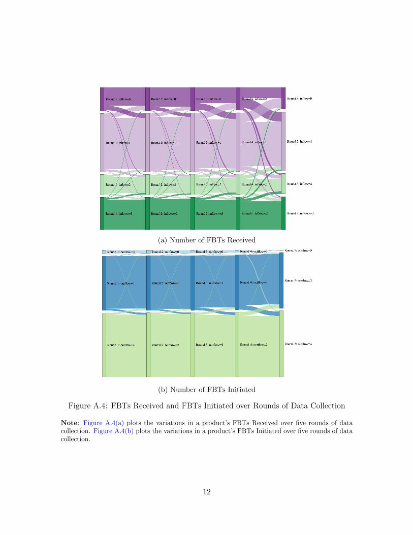
(a) Number of FBTs Received
(b) Number of FBTs Initiated
Figure A.4: FBTs Received and FBTs Initiated over Rounds of Data Collection
Note: Figure A.4(a) plots the variations in a product’s FBTs Received over five rounds of datacollection. Figure A.4(b) plots the variations in a product’s FBTs Initiated over five rounds of datacollection.
12

● 020
040
060
080
010
00
Pro
duct
ID
Round 1 Round 2 Round 3 Round 4 Round 5
Amazon StockoutAmazon Sells
(a) Amazon’s Presence at Product Level
● 020
040
060
080
010
00
Pro
duct
Pai
r ID
Round 1 Round 2 Round 3 Round 4 Round 5
FBT=YesFBT=No
(b) FBT Patterns at Directional Pair Level
Figure A.5: Data Variations over Rounds of Data Collection
Note: Figure A.5(a) plots the variations in Amazon’s presence over five rounds of data collectionfor 1,000 products selected by random sampling. Figure A.5(b) plots the variations in the recom-mendation patterns over five rounds of data collection for 1,000 product pairs selected by randomsampling; FBT is an indicator that whether one of the two products recommends the other one apair.
13
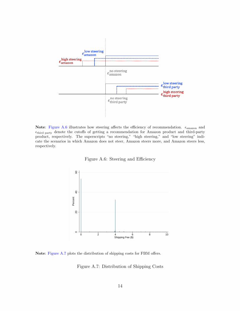
Note: Figure A.6 illustrates how steering affects the efficiency of recommendation. εamazon andεthird party denote the cutoffs of getting a recommendation for Amazon product and third-partyproduct, respectively. The superscripts “no steering,” “high steering,” and “low steering” indi-cate the scenarios in which Amazon does not steer, Amazon steers more, and Amazon steers less,respectively.
Figure A.6: Steering and Efficiency
020
4060
Per
cent
0 2 4 6 8 10Shipping Fee ($)
Note: Figure A.7 plots the distribution of shipping costs for FBM offers.
Figure A.7: Distribution of Shipping Costs
14

0.0
5.1
.15
Log
Sal
es
-15d -9d event +9d +15d
(a) Amazon’s Entry on Sales-.
1-.
08-.
06-.
04-.
020
Log
Mar
ket P
rice
-15d -9d event +9d +15d
(b) Amazon’s Entry on Market Price
-.2
-.15
-.1
-.05
0Lo
g S
ales
-15d -9d event +9d +15d
(c) Amazon’s Exit on Sales
0.0
5.1
.15
Log
Mar
ket P
rice
-15d -9d event +9d +15d
(d) Amazon’s Exit on Market Price
Figure A.8: Event Study of Amazon’s Presence
Note: Figure A.8(a) and Figure A.8(b) plot the coefficients of interest for fifteen days before andafter amazon’s entry in Equation A.1 using the log of sales and the log of market price as the outcomevariable, respectively. Figure A.8(c) and Figure A.8(d) plot the coefficients of interest for fifteendays before and after Amazon’s exit in Equation A.1 using the log of sales and the log of marketprice as the outcome variable, respectively. The vertical line indicates the time when Amazon entersor exits in the market. The coefficient for the 3 days before an presence is normalized to zero.
15

●
●
●
●
●
●
●
●
●
●
●
●
●
●
●
●
●
●
●
●
●
●
●●
●
●
●
●
●
Accessories
Baby
Bedding
Beverages
Boys
Cases, Holsters & Sleeves
Computers & Accessories
Dogs
Fan Shop
Girls
Hair Care
Health Care
Home & Kitchen Features
Kitchen & Dining
Kitchen & Dining Features
MakeupMen
Movies
Office & School Supplies
Outdoor Recreation
Pantry Staples
Skin Care
Sports & Fitness
Sports & Fitness Features
Styles
Subjects
TVVitamins & Dietary Supplements
Women
−0.01
0.00
0.01
0.02
−0.05 0.00 0.05 0.10 0.15 0.20Steering
Effe
ctiv
enes
s (n
on−
Am
azon
Min
us A
maz
on)
Note: Figure A.9 plots the loss of FBT efficiency (x axis) and the extent of steering (y axis) byproduct categories. The blue line indicates the linear fits and the gray area indicates the 95%confidence interval.
Figure A.9: Extent of Steering and Loss of FBT Efficiency across Product Categories
16

Table A.1: FBTs Initiated—OLS Regression
Dependent Var=log(Out + 1)(1) (2) (3) (4)
PLAT Referringi 0.061*** 0.061*** 0.050*** 0.050***(0.004) (0.006) (0.006) (0.009)
log(Q Referringi) 0.014*** 0.013***(0.003) (0.003)
log(P Referringi) -0.029*** -0.027***(0.009) (0.009)
Category Fixed Effects Y Y Y Y
No. of Observations 2,733,719 2,733,719 2,733,719 2,733,719Adjusted R-squared 0.072 0.081 0.082 0.090
Note: Table A.1 shows the regression results from Equation 3. Robust standard errors in parenthesesare clustered at the referring product’s category level.
Table A.2: FBTs Received of Amazon-Only Product—OLS Regression
Dependent Var=log(In + 1)(1) (2) (3) (4)
PLAT Only 0.236*** 0.248*** 0.125*** 0.136***(0.061) (0.061) (0.042) (0.042)
log(Q Recipienti) 0.107*** 0.106***(0.007) (0.007)
log(P Recipienti) -0.047*** -0.038***(0.006) (0.005)
Category Fixed Effects Y Y Y Y
No. of Observations 2,120,983 2,120,983 2,120,983 2,120,983Adjusted R-squared 0.012 0.016 0.102 0.104
Note: Table A.2 shows the regression results from Equation 1. PLAT Only is an indicator ofAmazon-only products. Robust standard errors in parentheses are clustered at the recipient prod-uct’s category level.
17

Table A.3: FBTs Initiated of Amazon-Only Product—OLS Regression
Dependent Var=log(Out + 1)(1) (2) (3) (4)
PLAT Only 0.058*** 0.065*** 0.045*** 0.053***(0.007) (0.009) (0.008) (0.010)
log(Q Referringi) 0.012*** 0.012***(0.003) (0.003)
log(P Referringi) -0.028*** -0.027***(0.008) (0.008)
Category Fixed Effects Y Y Y Y
No. of Observations 2,120,983 2,120,983 2,120,983 2,120,983Adjusted R-squared 0.053 0.061 0.060 0.067
Note: Table A.3 shows the regression results from Equation 3. PLAT Only is an indicator ofAmazon-only products. Robust standard errors in parentheses are clustered at the referring prod-uct’s category level.
Table A.4: Nonlinear Model: Variations in FBTs Received Depending on Amazon’sPresence
Dependent Var=FBTt
Linear Logit Probit(1) (2) (3)
PLAT Recipientt 0.080*** 0.763*** 0.448***(0.014) (0.125) (0.073)
log(Q Recipientt) 0.016*** 0.143*** 0.085***(0.003) (0.027) (0.016)
log(P Recipientt) -0.014*** -0.134*** -0.080***(0.004) (0.034) (0.016)
Product Pair Fixed Effects Y Y YCategory–Day Fixed Effects Y Y Y
No. of Observations 32,478,769 16,235,132 16,235,132
Note: Table A.4 reports coefficient estimates of interest from Equation 4 using alternative models.The dependent variable is an indicator of whether the referring product recommends the recipientproduct in a pair. Other coefficients and fixed effects are omitted for brevity. Robust standard errorsin parentheses are clustered at the recipient product’s category level. Significance levels: *(p<0.10),**(p<0.05), ***(p<0.01).
18

Table A.5: Additional Controls: Variations in FBTs Received Depending on Ama-zon’s Presence
Dependent Var=FBTt
(1) (2) (3)
PLAT Recipientt 0.081*** 0.083*** 0.083***(0.015) (0.015) (0.015)
log(Q Recipientt) -0.000 -0.000 0.000(0.002) (0.002) (0.002)
log(P Recipientt) -0.005 -0.006 -0.006(0.004) (0.004) (0.004)
log(Q Recipientt−5) 0.022*** 0.013*** 0.012***(0.003) (0.002) (0.002)
log(P Recipientt−5) -0.026*** -0.021*** -0.021***(0.003) (0.003) (0.002)
log(Q Recipientt−10) 0.017*** 0.007***(0.002) (0.002)
log(P Recipientt−10) -0.020*** -0.012***(0.004) (0.003)
log(Q Recipientt−15) 0.012***(0.001)
log(P Recipientt−15) -0.012***(0.004)
Product Pair Fixed Effects Y Y YCategory–Day Fixed Effects Y Y Y
No. of Observations 31,499,809 31,499,809 31,499,809Adjusted R-squared 0.400 0.401 0.401
Note: Table A.5 reports coefficient estimates of interest from Equation 4 controlling for lagged salesand prices. The dependent variable is an indicator of whether the referring product recommendsthe recipient product in a pair. Other coefficients and fixed effects are omitted for brevity. Robuststandard errors in parentheses are clustered at the recipient product’s category level. Significancelevels: *(p<0.10), **(p<0.05), ***(p<0.01).
19

Table A.6: Variations in FBTs Received Depending on Placebo Amazon’s Presence
Dependent Var=FBTt
(1) (2) (3)
PLAT Placebot 0.001 0.001 0.001(0.001) (0.001) (0.001)
log(Q Recipientt) 0.016*** 0.016***(0.003) (0.003)
log(P Recipientt) -0.020***(0.005)
Product Pair Fixed Effects Y Y YCategory–Day Fixed Effects Y Y Y
No. of Observations 31,289,416 31,289,416 31,289,416Adjusted R-squared 0.413 0.414 0.414
Note: Table A.6 reports coefficient estimates of interest from Equation 4 using placebo Amazon’spresence. The dependent variable is an indicator of whether the referring product recommends therecipient product in a pair. Other coefficients and fixed effects are omitted for brevity. Robuststandard errors in parentheses are clustered at the recipient product’s category level. Significancelevels: *(p<0.10), **(p<0.05), ***(p<0.01).
20

Table A.7: Price Perturbation: Variations in FBTs Received Depending on Amazon’sPresence
Dependent Var=FBTt
(1) (2) (3)$3.99 99th 99.9th
PLAT Recipientt 0.075*** 0.068*** 0.059***(0.013) (0.013) (0.014)
log(Q Recipientt) 0.016*** 0.016*** 0.016***(0.003) (0.003) (0.003)
log(P Recipientt) -0.019*** -0.020*** -0.018***(0.003) (0.003) (0.004)
Product Pair Fixed Effects Y Y YCategory–Day Fixed Effects Y Y Y
No. of Observations 32,375,268 32,375,268 32,375,268Adjusted R-squared 0.397 0.397 0.397
Note: Table A.7 reports coefficient estimates of interest from Equation 4 with price perturbation.Column (1), (2), and (3) increase the market price after Amazon experiences a stock out by $3.99,$11.85 (i.e., 99th percentile among third-party sellers’ shipping charges), and $37.87 (i.e., 99.9thpercentile among third-party sellers’ shipping charges), respectively. The dependent variable is anindicator of whether the referring product recommends the recipient product in a pair. Other coeffi-cients and fixed effects are omitted for brevity. Robust standard errors in parentheses are clusteredat the recipient product’s category level. Significance levels: *(p<0.10), **(p<0.05), ***(p<0.01).
21

Table A.8: Sales Perturbation: Variations in FBTs Received Depending on Amazon’sPresence
Dependent Var=FBTt
(1) (2) (3)10% 30% 100%
PLAT Recipientt 0.079*** 0.076*** 0.069***(0.014) (0.014) (0.013)
log(Q Recipientt) 0.016*** 0.016*** 0.016***(0.003) (0.003) (0.003)
log(P Recipientt) -0.014*** -0.014*** -0.014***(0.004) (0.004) (0.004)
Product Pair Fixed Effects Y Y YCategory–Day Fixed Effects Y Y Y
No. of Observations 32,375,268 32,375,268 32,375,268Adjusted R-squared 0.397 0.397 0.397
Note: Table A.8 reports coefficient estimates of interest from Equation 4 with sales perturbation.Columns (1), (2), and (3) increase the sales before Amazon experiences a stock out by 10%, 30%,and 100%, respectively. The dependent variable is an indicator of whether the referring productrecommends the recipient product in a pair. Other coefficients and fixed effects are omitted forbrevity. Robust standard errors in parentheses are clustered at the recipient product’s categorylevel. Significance levels: *(p<0.10), **(p<0.05), ***(p<0.01).
22

Table A.9: Variations in FBTs Received Depending on Third-Party Seller’s Presence
Dependent Var=FBTt
(1) (2) (3)
3Party Recipientt 0.003 0.003 0.003(0.003) (0.002) (0.002)
log(Q Recipientt) 0.022*** 0.021***(0.005) (0.005)
log(P Recipientt) -0.044***(0.008)
Product Pair Fixed Effects Y Y YCategory–Day Fixed Effects Y Y Y
No. of Observations 4,733,036 4,733,036 4,733,036Adjusted R-squared 0.399 0.400 0.400
Note: Table A.9 reports coefficient estimates of interest from Equation A.3. The dependent vari-able is an indicator of whether the referring product recommends the recipient product in a pair.Other coefficients and fixed effects are omitted for brevity. Robust standard errors in parenthesesare clustered at the recipient product’s category level. Significance levels: *(p<0.10), **(p<0.05),***(p<0.01).
Table A.10: Variations in FBTs Initiated Depending on Third-Party Seller’s Presence
Dependent Var=FBTt
(1) (2) (3)
3Party Referringt 0.001 0.001 0.001(0.001) (0.001) (0.001)
log(Q Referringt) -0.001*** -0.002***(0.000) (0.000)
log(P Referringt) -0.004(0.004)
Product Pair Fixed Effects Y Y YCategory–Day Fixed Effects Y Y Y
No. of Observations 5,566,200 5,566,200 5,566,200Adjusted R-squared 0.367 0.367 0.367
Note: Table A.10 reports coefficient estimates of interest from Equation 5 when we replace theindicator of Amazon’s presence with the indicator of a third-party seller’s presence. The dependentvariable is an indicator of whether the referring product recommends the recipient product in a pair.Other coefficients and fixed effects are omitted for brevity. Robust standard errors in parenthesesare clustered at the referring product’s category level. Significance levels: *(p<0.10), **(p<0.05),***(p<0.01).
23

Table A.11: Heterogeneous Recommendation Effectiveness Depending on CapacityConstraints
Dependent Var=log(Q Recipientt)(1) (2) (3) (4)
w/o Capacity Constraint w/ Capacity Constraint
log(Q Referringt) 0.296*** 0.297*** 0.358*** 0.359***(0.026) (0.026) (0.036) (0.036)
log(Q Referringt)×FBT -0.001 -0.001 0.007*** 0.007***(0.002) (0.002) (0.001) (0.001)
log(P Recipientt) -0.239*** -0.222**(0.072) (0.080)
Product Pair Fixed Effects Y Y Y YCategory–Day Fixed Effects Y Y Y Y
No. of Observations 6,201,687 6,201,687 24,337,366 24,337,366Adjusted R-squared 0.962 0.962 0.960 0.960
Note: Table A.11 reports coefficient estimates of interest from Equation 6 using recipient product’ssales as the outcome variable separately for products with and without a capacity constraint. Wedefine a product that recommends two products for at least one round of our data collection as acapacity-constrained product. Other coefficients and fixed effects are omitted for brevity. Robuststandard errors in parentheses are clustered at the recipient product’s category level. Significancelevels: *(p<0.10), **(p<0.05), ***(p<0.01).
24

Table A.12: Heterogeneous Extent of Steering Depending on Capacity Constraints
Dependent Var=FBTt
(1) (2) (3) (4) (5) (6)
w/o Capacity Constraint w/ Capacity Constraint
PLAT Recipientt 0.006 0.006 0.006 0.110*** 0.104*** 0.101***(0.007) (0.007) (0.007) (0.016) (0.015) (0.014)
log(Q Recipientt) -0.001 -0.001 0.020*** 0.020***(0.002) (0.002) (0.003) (0.003)
log(P Recipientt) 0.001 -0.017***(0.005) (0.004)
Product Pair Fixed Effects Y Y Y Y Y YCategory–Day Fixed Effects Y Y Y Y Y Y
No. of Observations 6,475,987 6,475,987 6,475,987 25,899,271 25,899,271 25,899,271Adjusted R-squared 0.474 0.474 0.474 0.374 0.375 0.375
Note: Table A.12 reports coefficient estimates of interest from Equation 4 separately for productswith and without a capacity constraint. We define a product that recommends two products forat least one round of our data collection as a capacity-constrained product. The dependent vari-able is an indicator of whether the referring product recommends the recipient product in a pair.Other coefficients and fixed effects are omitted for brevity. Robust standard errors in parenthesesare clustered at the recipient product’s category level. Significance levels: *(p<0.10), **(p<0.05),***(p<0.01).
Table A.13: Two-Sample Comparison Before v.s After Matching
Original Sample Matched Sample
PLAT Recipientt = 0 PLAT Recipientt = 1 PLAT Recipientt = 0 PLAT Recipientt = 1 %bias
Panel A: PLAT Referringt = 0log(Q Recipient) 8.535 9.568 9.501 9.529 -1.0log(Q Referring) 7.234 6.068 5.951 6.155 -8.1log(Count Recipient) 1.016 2.451 2.459 2.468 -1.0log(Count Referring) 0.953 1.295 1.308 1.264 5.8
Panel B: PLAT Referringt = 1log(Q Recipient) 8.587 8.965 8.986 8.838 6.1log(Q Referring) 7.402 7.464 7.517 7.578 -2.7log(Count Recipient) 1.323 2.225 2.193 2.193 0.0log(Count Referring) 1.757 1.901 1.869 1.833 4.5
Note: Table A.13 compares the means of recipient product’s sales, recipient product’s numberof sellers, referring product’s sales, referring product’s number of sellers for two groups. Panel Acompares the referring products that Amazon does not sell, Panel B referring products that Amazonsells. Column (1) compares the recipient products with and without Amazon in the original sample.Column (2) compares the recipient products with and without Amazon in the matched sample.
25

Table A.14: Heterogeneous Recommendation Effectiveness Depending on CapacityConstraints
Dependent Var=log(Q Recipientt)(1) (2) (3) (4) (5) (6) (7) (8)
w/o Capacity Constraints w/ Capacity Constraints
PLAT Referringt = 0 PLAT Referringt = 1 PLAT Referringt = 0 PLAT Referring= 1
FBTt × 1(PLAT Recipientt = 0) × log(Q Referringt) 0.005*** 0.005*** 0.007*** 0.007*** 0.012*** 0.012*** 0.017*** 0.017***(0.001) (0.001) (0.002) (0.002) (0.003) (0.003) (0.003) (0.003)
FBTt × 1(PLAT Recipientt = 1) × log(Q Referringt) 0.000 0.000 0.002 0.002 0.010*** 0.010*** 0.009*** 0.009***(0.002) (0.002) (0.001) (0.001) (0.001) (0.001) (0.002) (0.002)
1(PLAT Recipientt = 0) × log(Q Referringt) 0.303*** 0.305*** 0.347*** 0.351*** 0.282*** 0.284*** 0.334*** 0.338***(0.036) (0.037) (0.025) (0.025) (0.035) (0.035) (0.037) (0.037)
1(PLAT Recipientt = 1) × log(Q Referringt) 0.325*** 0.323*** 0.354*** 0.348*** 0.314*** 0.312*** 0.365*** 0.361***(0.030) (0.030) (0.023) (0.023) (0.027) (0.026) (0.025) (0.024)
log(P Recipientt) -0.218 -0.387*** -0.159* -0.332***(0.149) (0.059) (0.087) (0.080)
Product Pair Fixed Effects Y Y Y Y Y Y Y YCategory–Day Fixed Effects Y Y Y Y Y Y Y Y
No. of Observations 423,402 423,402 243,922 243,922 2,780,500 2,780,500 2,996,481 2,996,481Adjusted R-squared 0.952 0.952 0.957 0.958 0.955 0.955 0.954 0.955
Note: Table A.14 reports coefficient estimates of interest in Equation 9 using recipient product’ssales as the outcome variable separately for products with and without a capacity constraint. Wedefine a product that recommends two products for at least one round of our data collection as acapacity-constrained product. Other coefficients and fixed effects are omitted for brevity. Robuststandard errors in parentheses are clustered at the recipient product’s category level. Significancelevels: *(p<0.10), **(p<0.05), ***(p<0.01).
Table A.15: Extent of Steering and Loss of FBT Efficiency: Correlation across Prod-uct Categories
Dependent Var=Coef Lossc(1)
Coef PLATc 0.124***(0.036)
Constant -0.001(0.003)
No. of Observations 30Adjusted R-squared 0.273
Note: Table A.15 shows the coefficients in Equation A.4. The dependent variable is the loss of FBTefficiency (i.e., the difference in effectiveness estimates between recommending third-party productand recommending Amazon product). Robust standard errors are in parentheses. Significance levels:*(p<0.10), **(p<0.05), ***(p<0.01).
26